Zambia’s Child Grant Programme: 24-month impact report … · 24-month impact report on...

Zambia country case study report

Zambia’s Child Grant Programme:

24-month impact report on

productive activities and labour

allocation

i

Zambia’s Child Grant Programme: 24-month impact report on productive activities and labour allocation

Zambia country case study report

Silvio Daidone, Benjamin Davis, Joshua Dewbre

Food and Agriculture Organization of the United Nations (FAO) Rome, Italy

Mario González-Flores American University

Washington, D.C. USA

Sudhanshu Handa

University of North Carolina Chapel Hill, NC USA

David Seidenfeld

American Institutes for Research Washington D.C. USA

Gelson Tembo Palm Associates

Lusaka, Zambia

FOOD AND AGRICULTURE ORGANIZATION OF THE UNITED NATIONS

Rome, 2014

ii

The From Protection to Production (PtoP) programme, jointly with the United

Nations Children’s Fund (UNICEF), is exploring the linkages and strengthening

coordination between social protection, agriculture and rural development. The

PtoP is funded principally by the United Kingdom Department for International

Development (DFID), the Food and Agriculture Organization of the United

Nations (FAO) and the European Union.

The programme is also part of the Transfer Project, a larger effort together with

UNICEF, Save the Children and the University of North Carolina, to support the

implementation of impact evaluations of cash transfer programmes in sub-

Saharan Africa.

For more information, please visit PtoP website:

http://www.fao.org/economic/ptop

The designations employed and the presentation of material in this information product do not imply the expression of any

opinion whatsoever on the part of the Food and Agriculture Organization of the United Nations (FAO) concerning the legal

or development status of any country, territory, city or area or of its authorities, or concerning the delimitation of its frontiers

or boundaries. The mention of specific companies or products of manufacturers, whether or not these have been patented,

does not imply that these have been endorsed or recommended by FAO in preference to others of a similar nature that are not

mentioned.

The views expressed in this information product are those of the author(s) and do not necessarily reflect the views or policies

of FAO.

© FAO, 2014

FAO encourages the use, reproduction and dissemination of material in this information product. Except where otherwise

indicated, material may be copied, downloaded and printed for private study, research and teaching purposes, or for use in

non-commercial products or services, provided that appropriate acknowledgement of FAO as the source and copyright holder

is given and that FAO’s endorsement of users’ views, products or services is not implied in any way.

All requests for translation and adaptation rights, and for resale and other commercial use rights should be made via

www.fao.org/contact-us/licence-request or addressed to [email protected].

FAO information products are available on the FAO website (www.fao.org/publications) and can be purchased through

[email protected].

European Union

http://www.fao.org/economic/ptop

mailto:[email protected]

iii

Abstract

This report uses data from a 24-month randomized experimental design impact evaluation to

analyse the impact of the Zambia Child Grant Programme (CGP) on individual and household

decision making including labour supply, the accumulation of productive assets and other

productive activities. The general framework for empirical analysis is based on a comparison

of programme beneficiaries with a group of controls interviewed before the programme began

and again two years later, using both single and double difference estimators. The findings

reveal overall positive impacts of the CGP across a broad spectrum of outcome indicators and

suggest that the programme is achieving many of its intended objectives. Specifically, we find

strong positive impacts on household food consumption and investments in productive

activities, including crop and livestock production. The programme is associated with large

increases in both the ownership and profitability of non-farm family businesses; reductions in

household debt levels; increases in household savings; and concordant shifts in labour supply

from agricultural wage labour to better and more desirable forms of employment. The

analysis reveals important heterogeneity in programme impacts, with estimated magnitudes

varying over household and individual characteristics.

iv

Acknowledgments

Special thanks go to Leah Prencipe, Stanfeld Michelo and Amber Peterman for helpful

discussion and collaboration in data-collection efforts. We also thank participants at

workshops organized by the CGP impact evaluation steering committee and the Transfer

Project for invaluable discussion, comments and insight on the results. All mistakes and

omissions are our own. The results from this study form part of the integrated report on the

results of the Zambia CGP impact evaluation, reported in Seidenfeld, et al. 2013.

v

Abbreviations

AIR American Institutes for Research

CGP Child Grant Programme

CT Cash Transfer

DiD Difference-in-Differences

FAO Food and Agriculture Organization of the United Nations

IPW Inverse Probability Weighting

MCDMCH Ministry of Community Development, Mother and Child Health

PSM Propensity Score Matching

RCT Randomized Control Trial

SD Single Difference

UNICEF United Nations Children’s Fund

USD United States Dollars

ZMK

United States Dollars

Zambian Kwacha

vi

Contents

Abstract .................................................................................................................................... iii

Acknowledgments .................................................................................................................... iv

Abbreviations ............................................................................................................................ v

Executive summary ................................................................................................................ vii

1. Introduction ...................................................................................................................... 1

2. Research Design ................................................................................................................ 2

3. Analytical approach ......................................................................................................... 3

3.1. Difference in differences estimator .................................................................................... 3

3.2. Cross-sectional estimators .................................................................................................. 4

4. Data .................................................................................................................................... 5

4.1. Baseline .............................................................................................................................. 5

4.2. Evaluation sample, attrition and programme implementation ........................................... 7

5. Results and discussion ...................................................................................................... 8

5.1. Crop production .................................................................................................................. 8

5.2. Livestock production ........................................................................................................ 10

5.3. Consumption .................................................................................................................... 10

5.4. Non-farm business activities ............................................................................................ 11

5.5. Impact on credit and savings ............................................................................................ 11

5.6. Impact on labour supply ................................................................................................... 12

5.7. Impact on household income ............................................................................................ 13

6. Conclusions ..................................................................................................................... 14

References ............................................................................................................................... 15

Tables ....................................................................................................................................... 16

Figures ..................................................................................................................................... 34

vii

Executive summary

The Zambia Child Grant Programme (CGP) is one of the Government of Zambia’s

flagship social protection programmes. Implemented by the Ministry of Community

Development, Mother and Child Health (MCDMCH) since 2010, the programme currently

reaches 20 000 ultra-poor households with children under five years of age in three districts

(Shangombo, Kalabo and Kaputa). At the time of the baseline household survey for this study

in 2010, beneficiary households received 55 Kwacha (ZMK) a month (equivalent to around

USD 12) independent of household size, an amount subsequently increased to 60 ZMK a

month.

This research report uses data collected from a 24-month randomized experimental

design impact evaluation (2010 to 2012) to analyse the productive impact of the Zambia

CGP including food consumption, productive activities and investment, accumulation of

productive assets and labour allocation. Although the programme is designed to increase food

security and human capital development, with a focus on children under five, there are good

reasons to also expect impact on the economic choices of beneficiaries, who are primarily

agricultural producers.

First, we find robust evidence of a positive and statistically significant impact of the

programme on both food and non-food consumption. The impact is larger in magnitude

for food consumption and for smaller households (five or less members). The increase in food

consumption stems exclusively from purchases as both the share of households consuming

own-produced goods and the value of own-produced goods or received as gifts do not

increase as a consequence of the transfer. The variety of the diet has also increased: treated

households consumed significantly more quantities of cereals, pulses, meat, dairy/eggs,

oils/fats and sweet products as compared to control households. This is particularly true for

cereals and pulses in smaller-sized households.

Second, the programme has a significant impact on the accumulation of some

productive assets. Large and significant effects are found on both the share of households

owning animals and on the number of animals owned, especially for larger-sized households.

These effects are larger in magnitude for poultry. With respect to agricultural tools we

observe two distinct patterns: a significant positive impact on the share of households

accumulating agricultural implements with low initial values at baseline; and a significant

impact on the number of assets held for those implements already available at baseline by a

large share of households.

Third, CGP beneficiary households show an increase in savings and a tendency towards

paying off their loans. The impact is quite relevant for the share of households declaring to

accumulate savings in the form of cash, but in terms of the amounts the result is significant

only for smaller-sized households. We observe also a significant impact on the share of

households declaring to have made some loans repayments, and only for larger households is

this outcome significant in the absolute amount.

Fourth, the programme has a positive impact on agricultural activity. The CGP had a

large impact on increasing the size of operated land and the use of agricultural inputs,

viii

including seeds, fertilizer and hired labour, both on the share adopting those inputs and the

corresponding monetary amount, especially for smaller households. The increase in

agricultural input use led to higher production; we find a small yet significant increase in

maize and rice production for smaller households and a decrease in cassava production,

especially for larger households. The latter result however is consistent with the decline in

household consumption of tubers. The increase in production appeared to be primarily sold

rather than consumed on-farm; beneficiary households were more likely to sell their harvests

compared to non-beneficiaries, reflected in both the share of households selling cash crops

and the relative monetary value.

Finally, in term of labour supply, individuals from beneficiary households generally moved

out of agricultural wage labour and into off-farm family enterprises. The impact is significant

for both males and females, but is larger in magnitude for the latter. Further there is evidence

of a positive impact also for males in non-agricultural wage labour. These results are

consistent both in terms of probability of participation and intensity of labour. No effect is

found for on-farm or for child labour.

Overall, the study has provided direct evidence that the CGP programme influences the

livelihood strategies of the poor, with differential intensity across household size. The

programme has helped families increase food consumption and productive activities and

assets, including livestock holdings, which was among the six objectives of the programme.

Further it provided more flexibility to families in terms of labour allocation, especially for

women.

1

1. Introduction

This document constitutes the quantitative impact evaluation report on productive activities

and labour allocation of the Child Grant Programme (CGP) implemented by the Ministry of

Community Development, Mother and Child Health (MCDMCH), Government of Zambia.

The impact evaluation is implemented by the American Institutes for Research (AIR) which

has been contracted by the United Nations Children’s Fund (UNICEF) Zambia to design and

run a randomized control trial (RCT) for a three-year impact evaluation of the programme.

The results of this report are included in the overall two-year impact evaluation report

(Seidenfeld, et al. 2013).1

The CGP is an unconditional social cash transfer programme targeting any household with a

child under five years old in three districts (Kalabo, Kaputa and Shangombo) that had not

participated in a cash transfer programme in the past. Beneficiary households receive 60ZMK

a month (equivalent to USD 12), an amount deemed sufficient by the MCDMCH to purchase

one meal a day for everyone in the household for one month. The amount of the grant is the

same regardless of household size in order to reduce the incentive for misrepresenting

households’ membership, but also to reduce administrative costs associated with delivering

the transfer.

As with similar cash transfer programmes, the CGP aims to supplement household income,

increase education and health outcomes and improve the overall nutrition of household

members, especially children under five. Although the primary goal of the programme is to

build human capital and to improve food security, there are good reasons to believe that the

CGP can have impacts on the economic livelihoods of beneficiaries. Since the programme

targeted rural areas, the vast majority of programme beneficiaries depend heavily on

subsistence agriculture and live in places where markets for financial services (such as credit

and insurance), labour, goods and inputs are likely to be lacking or not function well.

Our hypothesis is that the liquidity and security of regular and predictable cash transfers can

increase productive and other income-generating investments, influence beneficiaries’ role in

social networks, increase access to markets and inject resources into local economies. These

impacts come through changes in individual and household behaviour (labour supply,

investments and risk management) and through impacts on the local economy of the

communities (social networks, labour and good markets, multiplier effects, etc.) where the

transfers operate.

Previous research in other sub-Saharan countries has shown that unconditional cash transfers

have an impact on agricultural and non-agricultural productive choices (Covarrubias et al.

2012; Asfaw et al. 2013). This report will provide impact estimates of the CGP on a range of

household and individual level outcomes. At the household level we examine consumption

and non-consumption expenditure, agricultural assets accumulation, agricultural production

and use of inputs, and saving behaviour. At the individual level we consider both adult and

child labour supply, overall as well as by gender.

1 Three tables (21, 24 and 29) included in this report are not found in Seindenfeld, et al. 2013.

2

2. Research Design

The CGP was implemented by the MCDMCH in 2010 in three of the poorest districts of the

country – Kalabo, Kaputa and Shangombo – that have the highest rates of mortality,

morbidity, stunting and wasting among children under five years of age. In addition to the

geographic targeting, the CGP used a categorical targeting approach in which any household

with a child under five years of age was eligible to receive the transfer. The transfers are made

every other month through a local pay-point manager. As with other transfer programmes

(such as Oportunidades in Mexico) the primary recipient of the transfer is the female in the

household that is considered to be the primary caregiver. In contrast to some of the largest

cash transfer programmes in the world, such as Oportunidades and Bolsa Familia, the CGP

does not impose any conditions attached to the cash transfer.

The CGP impact evaluation was designed as an RCT using a randomized phase-in method

(Duflo, Glennerster and Kremer 2008) that includes several levels of random selection. First,

90 out of 300 Community Welfare Assistance Committees (CWACs) in the three districts

were randomly selected and ranked through a lottery to be considered in the programme. In a

second phase CWAC members and Ministry staff identified all eligible households with at

least one child under the age of three living in these 90 randomly selected communities. This

resulted in more than 100 eligible households in each of the CWACs. After implementing a

power analysis to ensure the study was able to detect meaningful effects, 28 households were

randomly selected for inclusion in the evaluation from each of the 90 communities. This

yielded a final study sample of more than 2 500 households.

Baseline data collection was carried out before CWACs were randomly assigned to treatment

and control. Importantly, neither the households nor the enumerators knew who would benefit

first and who would benefit later. The randomization was concluded with the flip of a coin

and was carried out in public with local officials, Ministry staff and community members.

Half of the selected communities were assigned to treatment and were incorporated to begin

receiving benefits in December of 2010. The other half of the communities serve as the

controls, and they were scheduled to receive the programme at the end of 2013.

The CGP has six specific objectives:

1. Supplement and not replace household income;

2. increase the number of children enrolled in and attending school;

3. reduce the rate of mortality and morbidity among children under five years old;

4. reduce stunting and wasting among children under five years old;

5. increase the number of households owning assets such as livestock; and

6. increase the number of households that have a second meal a day.

3

3. Analytical approach

3.1. Difference in differences estimator

When panel data are available with pre- and post-intervention information, which is the case

with most of the outcome variables, the statistical approach we take to derive average

treatment effects of the CGP is the difference-in-differences (DiD) estimator. This entails

calculating the change in an indicator (Y), such as maize production, between baseline and

follow-up period for beneficiary (T) and non-beneficiary (C) households and comparing the

magnitude of these changes.

Two key features of this design are particularly attractive for deriving unbiased programme

impacts. First, using pre- and post-treatment measures allows us to net out unmeasured fixed

time-invariant family or individual characteristics (such as entrepreneurial drive) that may

affect outcomes. Second, using the change in a control group as a comparison allows us to

account for general trends in the value of the outcome. For example, if there is a general

increase in maize production because of higher rainfalls, deriving treatment effects based only

on the treatment group will confound programme impacts on production with the general

improvement in weather conditions.

The key assumption underpinning the DiD is that there is no systematic unobserved time-

varying difference between the treatment and control groups. For example, if plot quality for

the T group remains constant over time but the C group experiences on average deterioration

and erosion, then we would attribute a greater increase in agricultural production in T to the

programme rather than to this unobserved time-varying change in soil characteristic. In

practice the random assignment to T and C, the geographical proximity of the samples and the

rather short duration between pre- and post-intervention measurements, make this assumption

reasonable.

In large-scale social experiments like the CGP, it is typical to estimate the DiD in a

multivariate framework, controlling for potential intervening factors that might not be

perfectly balanced across T and C units and/or are strong predictors of the outcome (Y). Not

only does this allow us to control for possible confounders, it also increases the efficiency of

our estimates by reducing the residual variance in the model. The basic setup of the estimation

model is shown in equation (1):

Yit = β0 + β1Dit + β2Rt + β3(Rt* Di) + Σ βiZi +εit (1)

where Yit is the outcome indicator of interest; Di is a dummy equal to 1 if household i

received the treatment and 0 otherwise; Rt is a time dummy equal to 0 for the baseline and to

1 for the follow-up round; Rt* Di is the interaction between the intervention and time

dummies, and εit is the statistical error term. To control for household and community

characteristics that may influence the outcome of interest beyond the treatment effect alone,

we add in Zi, a vector of household and community characteristics to control for observable

differences across households at the baseline which could have an effect on Yit. These factors

are not only those for which some differences may be observed across treatment and control

at the baseline, but also ones which could have some explanatory role in the estimation of Yit.

4

As for coefficients, β0 is a constant term; β1 controls for the time-invariant differences

between the treatment and control; β2 captures changes over time; and β3 is the double

difference estimator which captures the impact of the programme.

3.2. Cross-sectional estimators

When panel data are not available, as is the case for some of our outcome variables that are

observed only at follow-up, a single difference (SD) estimator or propensity score matching

(PSM), or a combination of the two like the inverse probability weighting (IPW), can be

applied.

SD estimates impacts by comparing the mean values of the indicator of interest for the

recipients and the non-recipients. This estimator relies on the random assignment of the

households to the treatment and the control groups before the intervention takes place. Causal

effects estimates are unbiased since both potential outcomes and observed characteristics are

independent from the treatment. Equation (2) presents the regression equivalent of the SD

with covariates,

Yi = β0 + β1Di + Σ βiZi +εi (2)

where the estimated β1 coefficient is the causal effect of the programme, conditional on the Zi

vector of pre-treatment variables added to remove any potential bias arising from the

misallocation of the transfer. In this setting it is crucial to ensure that the controls Z are also

exogenous. Even with an RCT, it is easy to break the experimental design by introducing

endogeneity at the analysis stage.

Reweighting methods like the IPW are generally preferred for their finite sample properties

(smaller bias and more efficient) over PSM methods. Unsurprisingly, since randomization

worked well, results between the simple SD and the double robust IPW were very similar in

both significance and magnitude. In the results section therefore we present only the former

estimator.

5

4. Data

In order to evaluate the impact of the CGP this report uses baseline and 24-month follow-up

data. The core instrument is the household questionnaire, which is very similar in layout and

coverage to major national multitopic surveys in Zambia. The design of the instrument was

guided by three principles: i) inclusion of key indicators allowing the programme to be

assessed against stated objectives; ii) for all key indicators, use of questions from national

surveys to ensure comparability; and iii) manageable length to avoid interviewer or

respondent fatigue. Most of the instrument did not change between the two waves. However

at follow-up some edits were incorporated to facilitate the household-level analysis and a

study on the local economy. For the purposes of this research additional modules were added,

allowing better measures of labour supply and productive activities.

Special attention was paid to the process and the timing of data collection, making sure that it

was culturally appropriate, sensitive to Zambia’s economic cycle and consistently

implemented. For instance, the data at baseline and follow-up were conducted during the

same time of the year between September and October to be sure the data were not picking up

seasonal differences across the years. Importantly, given the objective and nature of the

programme, these months represent the beginning of the lean season when households face

the longest periods without a food harvest. The CGP aims to support households during a

period when they need the greatest support. The logic for collecting data during these months

is because this might be the period when the impacts of the programme are likely to be

largest.

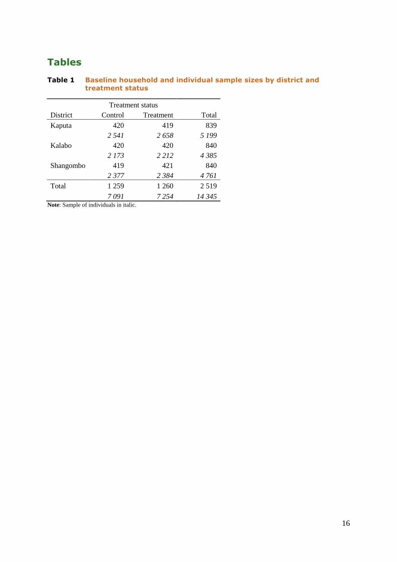
4.1. Baseline

The baseline data includes information for 2 519 households corresponding to 14345

individuals. Half of these households are in control communities and the other half are in

treated communities. The geographic distribution of households and individuals is shown in

Table 1, where it appears that households in Kaputa are bigger compared to the other two

districts, especially Kalabo. Additionally, treated households are slightly larger than the

control group.

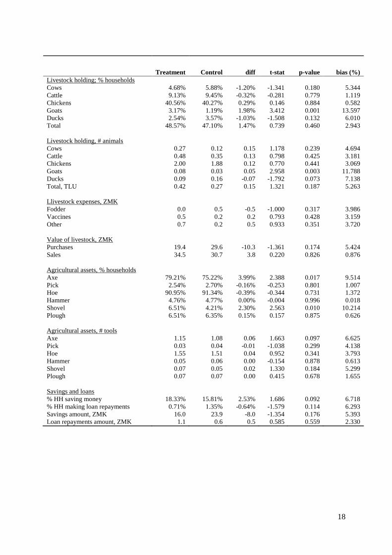
In the baseline report Seidenfeld and Handa (2011) demonstrate that randomization was

successful, as mean characteristics were balanced across groups. For the purpose of our study

however we test a different set of outcome measures which are related to productive

activities. With respect to household level variables we confirm that randomization has

worked since the vast majority of indicators are not statistically different at the conventional 5

percent significance level, with 10 exceptions out of 71 (see Table 2). Four indicators have

standardized differences greater than 10, but they are all below 15. Given the large sample

size we have power to detect very small and substantively meaningless differences.

Besides checking for statistical equivalence between groups, the baseline provides a clear

snapshot of the livelihoods in the targeted rural areas. A large majority of programme-eligible

households are agricultural producers (almost 80 percent). By far the most important crop is

maize; about a third of households produce cassava and 20 percent rice; followed by a

smattering of millet, groundnut and sweet potatoes (see Table 3). As can be seen in Figure 1,

6

each district has quite different crop production patterns. Looking at the share of households

producing each crop, Kaputa has mixed maize and cassava production (with a larger share of

cassava), while Kalabo has mixed maize and rice production (with a larger share of rice).

Maize dominates in Shangombo. In terms of available agricultural land, cropped areas are on

average small among households in this sample, at just over half a hectare for those producing

crops (see Table 4). Average land sizes are relatively similar across districts with somewhat

higher values in Kalabo. Minor differences between treatment and controls households within

districts are also discernible.

Not surprisingly, given the small land cropping sizes most crop production is for household

consumption, though differences emerge among crops. We look at this from two dimensions.

First, in Table 5 we see that overall 29 percent of crop producers at baseline sold some part of

their harvest. By crop, however, this ranges from 19 and 16 percent for maize and cassava to

50 percent for rice, which means that rice to some extent functions as a cash crop in Kalabo

and particularly in Kaputa (65 percent of rice producers sold some of their crop).

Second, in Figure 2 we see the distribution of maize use by district and by treatment and

control. In all three districts the largest share of production goes to household consumption,

but a non-trivial share (around 20 percent) is stored or given out as reimbursement. In Kaputa

twenty percent of the harvest is sold. Very small amounts are used as by-products and as

inputs to animal production.

Households in the baseline sample have relatively low levels of livestock assets. Less than

half of all households have any kind of livestock and most of these households have only

chickens. Only 5 percent of households have milk cows, and 10 percent have other kinds of

cattle. For those that own milk cows, other cattle and goats, the average herd size is 3.7, 4.5

and 2.5 animals respectively.

Most producers used traditional production systems. Only 28 percent of crop producers used

purchased inputs (Table 6). Most of these inputs (16 percent of producers) were seeds; only 1

percent used any kind of chemical input (fertilizers or pesticides). Some differences between

treatment and control households do emerge at the district level though the numbers are small.

Most households in the sample have basic agricultural implements: over 90 percent of

households have a hoe and 79 percent an axe. From there it drops to less than 10 percent with

a shovel or a plough.

Adult labour supply varies by gender (Table 7). At baseline women are more involved in

nonfarm self-enterprise activities (17 to 8 percent) and as homemakers, while men are more

involved in agricultural activities and particularly in fishing. Both men and women participate

equally in wage activities. Significant differences between treatment and control households

do emerge in a number of categories for males, though the differences are not of great

magnitude.

Child labour is common among the households in this sample. Over 50 percent of children

aged five to 18 are involved in labour activities (Table 8), almost all of which are unpaid. And

an even a large share – 38 percent – of younger children (aged five to 10) “normally” work.

This share increases dramatically by age, with 69 percent of 11-13 year olds and 77 percent of

14-18 year olds.

7

For those children who worked at baseline, the time commitment is significant as seen in

Table 9. Children worked on average 25 hours of unpaid labour in the last two weeks prior to

survey – reaching 35 hours for the oldest children. As the survey did not take place during a

period of high agricultural demand for child labour, the numbers may not reflect increased

seasonal demand for children’s labour, paid or unpaid. Most of the relatively few cases of

paid labour involved casual labour and farming (not reported in the Table).

4.2. Evaluation sample, attrition and programme implementation

Of the 2 519 target households, 2 298 were re-interviewed at follow-up, entailing an attrition

rate of 8.8 percent. Mobility, the dissolution of households, death and divorce can cause

attrition and make it difficult to locate a household for a second data collection. Sometimes

households can be located and contacted but they may refuse to respond. Attrition causes

problems within an evaluation because it not only decreases the sample size (leading to less

precise estimates of programme impact) but also may introduce selection bias to the sample

which will lead to incorrect programme impact estimates or change the characteristics of the

sample and affect its generalizability.

Seidenfeld et al. (2013) investigated in detail both differential and overall attrition. The

former relates to baseline characteristics between treatment and control households that

remain at follow-up. The latter instead looks at similarities at baseline between the full sample

of households and the non-attriters. They did not find any significant differential attrition after

twenty-four months, meaning that the benefits of randomization are preserved. The

differences in overall attrition are primarily driven by the lower response rate in Kaputa

district.

For the purposes of this report we extended the attrition analysis in two directions: i) we

looked at both differential and overall attrition in terms of outcome indicators of interest for

this study; and ii) we assessed attrition randomness within the multivariate framework of a

logit model. With respect to the former point we strongly confirmed results achieved by

Handa et al. For instance, compared to baseline differences between treated and control

groups already shown in Table 2, we detect only two additional outcome indicators as

statistically different at conventional 5% level. Further, when comparing the full vs reduced

sample at baseline, no indicator is statistically different at 5%.

In order to evaluate attrition randomness in a multivariate framework we have run two simple

logit models: 1) in the first we included the household level variables analysed by Handa et

al. for overall attrition (both controls and outcomes); 2) in the second specification we added

other outcomes related to productive activities, the treatment indicator, community level

prices and, following Maluccio (2004), quality of first-round interview variables such as a

dummy for revisit and length of interview. The issue is whether there is unobserved

heterogeneity driving attrition which is related to programme impacts that could lead our

working sample to give biased estimates. However apart from a significant effect of

(exogenously determined) food prices, we do not find any significant effect for the remaining

covariates except the dummy variable for Kaputa district. The treatment indicator is not

statistically significant and this reinforces the idea that attriters are balanced across the two

groups. As a further robustness check, we predicted attrition probabilities for the two logit

models and from them we computed inverse probability weights which we used in the impact

8

analysis. The unweighted and weighted estimates provided identical results in terms of sign

and significance for the different outcome indicators, while differences in impact magnitude

weres negligible. In the results section we refer to the weighted estimates on the sample

remaining at 24-month follow-up.

As far as the implementation of the programme is concerned, the main findings from

Seidenfeld et al. (2013) suggest that overall CGP has been successful: beneficiaries received

the designated amount on time, accessing the money with ease and without any cost. Only

twenty beneficiary households responding at follow-up declared they had never received a

payment, i.e. less than 2% of the beneficiaries. Efficient funds disbursement is crucial in cash

transfer programmes, since payment regularity and minimal private costs in terms of

accessing money accentuate programme effectiveness. Further, contamination does not

appear to be a significant issue: thirty-five control households declared having received CGP

payments and thirty-two of them reported having at least one household member who was

currently a beneficiary. There could be a number of reasons for this occurrence: control

households received a payment because they moved to a new area and found a way to register

in a neighbouring treatment CWAC. It is also possible that respondents simply lied about

receiving the payment or misunderstood the question. In our impact estimates we decided to

keep these households in order to avoid introducing selection bias that we cannot account for.

This may lead to a lower impact estimate rather than a pure ATT. Our panel estimation

sample therefore is based on 2 298 households responding both at baseline and at follow-up.

5. Results and discussion

In this section we discuss the average treatment effects of the Zambia CGP programme on the

treated households over six broad groups of outcome variables – crop production, livestock

production, consumption, non-agricultural business activities, savings/credit decisions and

labour supply. When the baseline information is available for a given outcome variable we

employ a DiD estimator in a multivariate framework. However, when baseline information is

missing, we use the single difference estimator. All standard errors reported in the tables are

clustered at CWAC level.

5.1. Crop production

We look at various dimensions of the productive process in order to ascertain whether

households have increased spending in agricultural activities, including crop production and

crop input use. Overall, in terms of these direct impacts on crop activity, we find positive and

significant impacts on area of land operated, overall crop expenditures, the share of

households with expenditures on inputs (Table 10), and expenditure on seeds, fertilizer, hired

labour and other expenditures (

Table 11). The CGP increases the amount of operated land by 0.18 hectares (a 36 percent

increase from baseline), and the programme has led to an increase of 18 percentage points in

the share of households with any input expenditure, from a baseline share of 23 percent. This

increase was particularly relevant for smaller households (22 percentage points) and included

spending on seeds, fertilizer and hired labour. The increase of 14 percentage points in the

proportion of small households purchasing seeds is equivalent to more than a doubling in the

share of households. Small beneficiary households spent ZMK 42 more on crop inputs than

9

the corresponding control households, including ZMK 15 on hired labour. This equals three

times the value of the baseline mean for overall spending and four times for hired labour.

Similarly, we see a positive impact on ownership of agricultural tools, but with two distinct

patterns: a positive impact of between 3 to 4 percentage points on the share of households

accumulating agricultural implements with low initial values at baseline (less than 10 percent

at baseline), such as hammers, shovels and ploughs (Table 12); and a significant impact on

the number of assets held, for those implements already widely available at baseline (up to

approximately 90 percent of households at baseline), such as axes and hoes (Table 13). The

impact on hammers, shovels and ploughs is concentrated among larger-sized households (7

percentage points in the case of hammers, from a baseline of 6 percent).

Did the increase in input use and tools lead to an increase in crop production? We focus

primarily on the three most important crops (maize, cassava and rice), as well as aggregating

all production by value of total harvest.2 First, the programme facilitated shifts in production

compared to control households (Table 14). The share of (large) beneficiary households

planting maize increased by 8 percentage points (from a baseline of 58 percent), while the

share of small beneficiary households planting rice increased by 4 percentage points (from a

baseline of 17 percent). The share of all households producing groundnuts – a relatively

minor crop (5 percent at baseline) – increased by 3 percentage points.

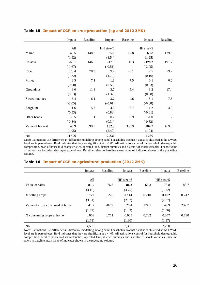
Aggregating all output by value, we find that the CGP had a positive impact (at the 10 percent

level) in the value of all crops harvested – ZMK 146, an approximately 37 percent increase

from baseline (Table 15). The impact rises to ZMK 182 for smaller households and is not

significant for larger households. We find few significant impacts, however, on the output of

specific crops. The impact results regarding maize are large and in the right direction, but not

quite significant. The results are similar for rice, though in this case for small households the

positive impact is significant at 10 percent. Larger households had significantly lower

production of cassava (129 kg, from a baseline of 179 kg). The latter result is consistent with

the decline in consumption of tubers found in the food consumption module.

Why is there a significant impact on the value of aggregate production yet far less of a clear

story of impact on specific crops? It could be the result of a diffuse increase in production

across crops. Differential crop price increases between treatment and control households may

have played a role, but we find possible indication of this only in the case of the price of rice.3

Note also that no production data were collected on fruits and vegetables, though from the

consumption model there is a significant increase in the share of households consuming fruits

and vegetables from home production. Finally, while households used more inputs in

production they may not be using them in the most efficient manner – efficiency analysis is a

topic for further research.

Along with an increase in the value of crop production, a larger share of beneficiary

households marketed their crop production (an increase of 12 percentage points, from a

2 The value of total harvest is the product of harvest quantity and the median unit price; the latter is computed from crop sales

at district level and if missing, at the level of all three districts. 3 We compared sale prices for each crop in the production module across time after inflating the reported values in 2010 to

2012 using the all-Zambia CPI. Simple t-tests show that only the price of rice is significantly higher in 2012 compared to

2010, and significantly different between treatment and control households.

10

baseline of 22 percent). The average value of sales among all crop producing households was

also larger for beneficiary households (ZMK 82, over double the baseline value of ZMK 77),

though in the case of larger households the impact is significant only at 10 percent. The

increase in market participation was driven by maize production in Kaputa, and both maize

and rice production in Kalabo. At the same time, the share of households consuming some

part of their harvest increased by 6 percentage points (significant at the 10 percent level, as

seen in Table 16) which comes from increased groundnut and rice consumption of home

production (not shown). This result is compatible with the analysis of the last two weeks of

consumption reported in the consumption module, where the share of consumption from

home production increases with CGP participation but is not statistically significant.

5.2. Livestock production

The CGP had a positive impact on the ownership of a wide variety of livestock both in terms

of share of households with livestock (a 21 percentage point increase overall, from 48 percent

at baseline; Table 17) and in the total number of goats and poultry (an increase in 0.14 goats,

0.2 ducks and 1.23 chickens, from baseline values of 0.05, 0.13 and 1.99 respectively; Table

18). Both small and large beneficiary households increased livestock ownership, but the

impacts were particularly strong for large households. The share of large households with

livestock increased 27 percentage points from a base of 54 percent (compared to 16

percentage points for small households), including 5 and 21 percentage point increases in the

ownership of milk cows and chickens respectively (compared to non-significant results for

small households). In terms of numbers of livestock, the impact was more balanced between

small and larger households. Small household beneficiaries obtained more goats, larger

households more ducks and overall, small households accumulated more animals as measured

in Tropical Livestock Units (TLU)4 though significant only at the 10 percent level.

Overall, beneficiary households had a significantly larger volume of purchases and sales of

livestock compared to control households (Table 19). This increase in volume is not

significant for smaller households; for larger households, the joint volume of sales (ZMK

109) and purchases (ZMK 73) is over twice as large as at baseline. In contrast to crop input

use, no impact is found on expenditure on inputs for livestock production, including

vaccinations and other expenditures. With respect to fodder we observe a significant (at 10

percent) positive impact for smaller-sized households, but given data limitations we are

unable to assess whether home produced fodder is substituting for purchased fodder and thus

this variable may underestimate the overall increase in fodder use, particularly for larger

households who have more productive capacity.

5.3. Consumption

Table 20 contains the impact estimates on adult equivalent total, food and non-food

consumption. Approximately 80 percent of the positive and significant increase in total

consumption goes towards food, a finding consistent with other cash transfer programmes. As

shown in

4 The TLU conversion factors are based on the average weight of animal species and aggregation of livestock into a single

index.

11

Table 21, the increase in food consumption stems from an increase in purchases of food, not

from increases in own production, especially in smaller households. This means that the share

of food consumption purchased rose from 43.5 to around 54 percent because of the

programme. For maize, not only did purchases increase, but also consumption from own

production, for which we detect a significant increase of around ZMK 1.15 (results not

reported). Further, similar results are obtained for the share of households consuming in each

food category: a 5.7 and 4.2 percentage point increase in consumption of maize and rice is

observed, but only with a ten percent significance level (results not shown).

5.4. Non-farm business activities

Households benefitting from the CGP are significantly more likely to have a non-farm

business. The average treatment effect ranged from 16 to 18 percent for small and large

households respectively (Table 22). In addition to their greater likelihood of running a

business, CGP households operated enterprises for longer periods (1.5 months more on

average) and more profitably – earning about ZMK 69 more than control businesses. Results

also suggest the programme is enabling businesses to accumulate physical capital. Beneficiary

households are 5 percentage points more likely to own assets and have substantially larger

holdings (as judged by value) though the latter is not statistically significant. Estimated

magnitudes are greater for larger households across all enterprise-related outcomes.

With respect to the financing of non-farm business activities and excluding CGP, some

households use CGP as a source of capital. Further, after CGP implementation larger

households are significantly more likely to reinvest proceeds from their non-farm activities,

the impact being 4.5 percentage points (results not shown). However compared to control

households beneficiaries are not more likely to attract additional resources, neither through

loans from institutions or people, nor by using own savings or wage labour earnings.

5.5. Impact on credit and savings

Households benefitting from CGP show an increase in savings and a tendency towards paying

off their loans (Table 23).5 The impact in terms of the share of households declaring to

accumulate savings in the form of cash is large (+24 percent) and in terms of the amounts the

result is larger for smaller sized households. We observe also a significant impact on the share

of households declaring to have made some loans repayments (1.7 percent), and only for

larger households is this outcome significant in the absolute amount. The DiD estimates are

mirrored by the results on the propensity of purchase on credit and for loan application (Table

24). In the former case, results are negative but not statistically significant while for the latter

impact estimates are strongly negative for larger households. We might interpret this result as

an indication of a generally negative attitude of the targeted population towards being in debt.

5 This table does not exactly match Table 10.2 (Savings and Future Outlook) in Seidenfeld et al. 2013. We include loan

repayments and use the reported amount, while they use the log of savings. We have estimated a 24 percentage points

increase in the share of households saving, while Seidenfeld et al. 20123, estimated a 20.1 percentage points.

12

5.6. Impact on labour supply

The changes in household economic activities brought on by the CGP necessarily imply

changes in labour activities of individual household members, the main input to household

livelihoods, including wage labour and agricultural and non-agricultural enterprises. Overall,

we find a significant shift from agricultural wage labour to family agricultural and non-

agricultural businesses, in correspondence with the increases in household level economic

activities brought on by receipt of the CGP transfer.

The CGP led to a 9 percentage point decrease in the share of households with an adult

engaged in wage labour, from 59 percent at baseline (Table 24). The impact was much

stronger for households with females of working age – a decrease of 14 percentage points

compared with no significant impact on households with males of working age.6

In terms of types of employment the reduction in wage labour took place primarily in

agricultural wage labour, with an 8 percentage point reduction for households with male

labour and a 17 percentage point reduction for households with female labour (Table 25).

This result was expected as agricultural wage labour is generally considered the least

desirable labour activity of last resort, and when liquidity constrained, households may be

obliged to overly depend on it. The CGP also led to a reduction in labour intensity in terms of

days of agricultural wage labour, both overall (14 days fewer per year) and for females (12

days fewer per year). The reduction in agricultural wage labour is also reflected in the yearly

value of household earnings which was reduced by ZMK 93 for households with female

labour. On the other hand, while the programme did not have a significant impact on

participation in non-agricultural wage labour (although the coefficients are positive), it did

have a significant impact in terms of increasing earnings derived from this kind of work, both

overall (ZMK 471) and for households with female labour (ZMK 154). This significant

impact stems from a small (less than one percentage point) increase in permanent non-

agricultural wage employment for females.

If not working in agricultural wage labour, what did the male and female adults in beneficiary

households do with their time? Part of that time was spent working in the family’s non-farm

enterprise – the CGP led to a 16 percentage point increase in the share of households that

engaged in labour dedicated to non-farm enterprise activity, with an average increase of 1.57

days a week in terms of intensity (Table 26). The impact is somewhat higher for female

labour (16 percentage points and 0.98 days a week in terms of intensity compared to 12

percentage points and 0.62 days a week).

We would have expected the CGP to have led to an increase in the intensity of on-farm

labour, given the productive impacts described above. Indeed households with male labour

spend an extra 13 days in own farm agricultural activities (Table 27). Overall, beneficiary

households spend an extra 20 days in own farm labour (significant at the 10 percent level).

Finally adults may also increase their time spent in domestic chores, or child care, or simply

6 In this analysis we join together permanent and temporary labour since only 3 percent of households have access to

permanent employment. Permanent workers typically refer to employees with paid leave entitlements in jobs or work

contracts of unlimited duration, including regular workers whose contract last for 12 months and over. Temporary employees

usually have an expected duration of a main job of less than one year, carrying out seasonal or casual labour.

13

leisure, but data were not collected on these common household activities which can all lead

to an increase in family well-being.

Finally with respect to child labour, the survey instrument dedicated a full section on the

economic activities performed by children aged five to 18 at both baseline and follow-up,

allowing us to use DiD estimates (Table 28). Overall, the programme has not had any impact

on children’s work, in either paid or unpaid activities. Given programme impacts on

household productive activities and adult labour supply along with findings on reducing child

labour from cash transfer programmes in other countries, these results suggest the need for

further research.

5.7. Impact on household income

Lastly, in this section we focus our analysis on the impact of the CGP on the composition of

household income which is expressed as the share of a given source in annual total gross

income. In Table 29 we provide the impact of the CGP on the shares of household income

sources. Three results emerge from this set of estimates: i) there is a large increase in the

share of income coming from non-farm enterprises (14.3 percentage points); ii) a considerable

decline of the relative importance of wage employment income, falling by 10 percentage

points; and iii) a statistically significant rise of income from livestock sources and a drop in

other types of transfers, excluding the CGP. Both of the latter results are however small in

magnitude. The reduction in wage employment is concentrated almost exclusively within the

agricultural sector. Further all these results are substantially homogeneous, with minor

differences in magnitude by household size.

14

6. Conclusions

This report uses data collected between 2010 and 2012 in three of the poorest districts of

Zambia in order to assess whether an unconditional cash transfer, the CGP, targeting very

poor households can have an effect on agricultural production and livelihood options. The

CGP was implemented using an RCT phased-in approach where half of 90 communities were

assigned to receive the treatment in 2010, while the other half were to receive the programme

starting in 2013. The CGP used a combination of geographic and categorical targeting to

identify households with at least one child under the age of three. The CGP does not impose

any conditions attached to the cash transfer. The programme has been shown to have a

positive impact over a number of household and child welfare indicators, including

consumption, dietary diversity, health and schooling (Seidenfeld et al. 2013).

The results found in this paper present a promising picture in terms of the impact of the

programme on investments in productive assets, input use and agricultural production.

Households invested more in livestock: large and significant effects are found on both the

share of households owning animals and on the number of animals owned, especially for

larger-sized households. Further, the CGP is facilitating the purchase and/or increased use of

agricultural inputs, especially land, seeds, fertilizers and hired labour, both on the share

adopting those inputs and the corresponding monetary amount, especially for smaller

households.

The increase in the use of agricultural inputs led to expansion in the production of maize and

rice, though statistically significant only for smaller-sized households – and beneficiary

households reduced the production of cassava. In contrast with cash transfer results from

other countries such as Malawi and Kenya, the increase in agricultural production did not lead

to an increase in consumption of goods produced on farm, but instead to more market

participation. More detailed analysis can be carried out to ascertain whether these average

impacts are similar across different types of agricultural producers.

The programme has had a positive and significant impact in improving the livelihood position

and options of treated households which after intervention derive a much greater share of

income from off-farm enterprises and a much lower share from wage employment, especially

temporary agricultural labour. Taken together with adult labour supply response, these results

suggest that, for some beneficiary households, the programme satisfies a cash flow need that

was otherwise met through less preferred casual agricultural work and thus allowing

households to concentrate on household business activities, whether in agriculture or off farm.

15

References

Asfaw, S., Covarrubias, K., Davis, B., Dewbre, J., Djebbari, H., Romeo, A. & Winters, P.

2012. Analytical framework for evaluating the productive impact of cash transfer

programmes on household behavior. Methodological guidelines for the From Protection to

Production Project, paper prepared for the From Protection to Production project, FAO,

Rome.

Covarrubias. K., Davis. B. & Winters, P. 2012. From Protection to Production: Productive

Impacts of the Malawi Social Cash Transfer Scheme. In Journal of Development

Effectiveness, 4(1): 50-77.

Caliendo, M. & Kopeinig, S. 2008. Some practical guidance for the implementation of

propensity score matching. In Journal of Economic Surveys, 22(1): 31–72.

Duflo, E., Rachel Glennerster, R. & Kremer, M. 2008. Using Randomization in Development

Economics Research: A Toolkit. In T. P. Schultz & J. Strauss, eds. Handbook of

Development Economics, vol. 4, , pp. 3895–3962. Amsterdam: North-Holland.

Maluccio, J. 2004. Using Quality of Interview Information to Assess Nonrandom Attrition

Bias in Developing-Country Panel Data In Review of Development Economics, 8(1): 91–

109.

Rosenbaum, P. & Rubin, D. 1998. The central role of the propensity score in observational

studies for causal effects. In Biometrika, 70(1): 41-55.

Seidenfeld, D. & Handa, S. 2011. Zambia’s Child Grant Program: Baseline Report.

Washington, D.C. American Institutes of Research. November.

Seidenfeld, D., Handa, S. & Tembo, G. 2013. 24-Month Impact Report for the Child Grant

Programme. Washington, D.C. American Institutes of Research, September.

Smith, J.A. & Todd, P. E. 2005, Does matching overcome LaLonde’s critique of on

experimental Estimators? In Journal of Econometrics 125: 305–353.

16

Tables

Table 1 Baseline household and individual sample sizes by district and

treatment status

Treatment status

District Control Treatment Total

Kaputa 420 419 839

2 541 2 658 5 199

Kalabo 420 420 840

2 173 2 212 4 385

Shangombo 419 421 840

2 377 2 384 4 761

Total 1 259 1 260 2 519

7 091 7 254 14 345 Note: Sample of individuals in italic.

17

Table 2 Baseline household outcomes

Treatment Control diff t-stat p-value bias (%)

Consumption per adult equivalent

Food 53.3 50.4 3.0 1.555 0.120 6.198

Non-food 17.6 16.8 0.7 1.137 0.255 4.533

Own-produced 21.0 19.2 1.7 1.431 0.152 5.704

Income sources

HH farming 76.83% 78.95% -2.13% -1.286 0.199 5.123

HH herding livestock 49.29% 47.42% 1.87% 0.937 0.349 3.735

Any HH member in waged labor 11.11% 10.25% 0.86% 0.703 0.482 2.800

HH received any transfer 30.00% 26.61% 3.39% 1.890 0.059 7.531

Production

Value of harvest 403.8 398.1 5.7 0.211 0.833 0.840

Value of sales 73.4 80.4 -7.0 -0.435 0.664 1.732

HH selling crops 20.48% 25.10% -4.62% -2.769 0.006 11.034

Value of own consumption 207.1 206.4 0.7 0.065 0.948 0.258

Quantity harvested, kg

Maize 153.1 143.9 9.1 0.602 0.548 2.397

Cassava 159.3 136.0 23.2 1.360 0.174 5.421

Rice 75.5 82.2 -6.7 -0.586 0.558 2.334

Millet 6.0 8.7 -2.7 -1.539 0.124 6.131

Groundnut 9.2 13.5 -4.4 -1.292 0.197 5.147

Sweet potatoes 5.1 8.3 -3.2 -1.847 0.065 7.358

Sorghum 3.4 7.6 -4.2 -1.577 0.115 6.282

Other beans 1.0 1.0 0.0 0.018 0.986 0.070

% households harvesting

Maize 55.48% 55.20% 0.27% 0.138 0.890 0.550

Cassava 24.21% 27.64% -3.43% -1.968 0.049 7.841

Rice 15.71% 16.60% -0.89% -0.604 0.546 2.407

Millet 5.71% 6.59% -0.88% -0.917 0.359 3.654

Groundnut 4.29% 5.32% -1.04% -1.216 0.224 4.844

Sweet potatoes 3.81% 5.08% -1.27% -1.551 0.121 6.181

Sorghum 2.62% 4.37% -1.75% -2.393 0.017 9.535

Other beans 0.95% 1.67% -0.72% -1.580 0.114 6.294

Input use, ZMK

Operated land , ha 0.50 0.49 0.00 0.109 0.914 0.433

Seeds 6,521 5,892 629 0.652 0.515 2.598

Hired labour 12,056 2,143 9,913 2.199 0.028 8.764

Pesticides 0 50 -50 -1.095 0.274 4.363

Fertilizers 1,517 1,313 204 0.266 0.790 1.059

Other 7,285 4,930 2,355 1.512 0.131 6.028

Input use, % households

Seeds 13.10% 13.26% -0.17% -0.126 0.900 0.500

Hired labour 3.73% 2.14% 1.59% 2.358 0.018 9.397

Pesticides 0.00% 0.16% -0.16% -1.415 0.157 5.639

Fertilizers 1.03% 0.79% 0.24% 0.626 0.531 2.496

Other 10.48% 10.41% 0.07% 0.058 0.953 0.232

(Continued)

18

Treatment Control diff t-stat p-value bias (%)

Livestock holding; % households

Cows 4.68% 5.88% -1.20% -1.341 0.180 5.344

Cattle 9.13% 9.45% -0.32% -0.281 0.779 1.119

Chickens 40.56% 40.27% 0.29% 0.146 0.884 0.582

Goats 3.17% 1.19% 1.98% 3.412 0.001 13.597

Ducks 2.54% 3.57% -1.03% -1.508 0.132 6.010

Total 48.57% 47.10% 1.47% 0.739 0.460 2.943

Livestock holding, # animals

Cows 0.27 0.12 0.15 1.178 0.239 4.694

Cattle 0.48 0.35 0.13 0.798 0.425 3.181

Chickens 2.00 1.88 0.12 0.770 0.441 3.069

Goats 0.08 0.03 0.05 2.958 0.003 11.788

Ducks 0.09 0.16 -0.07 -1.792 0.073 7.138

Total, TLU 0.42 0.27 0.15 1.321 0.187 5.263

Llivestock expenses, ZMK

Fodder 0.0 0.5 -0.5 -1.000 0.317 3.986

Vaccines 0.5 0.2 0.2 0.793 0.428 3.159

Other 0.7 0.2 0.5 0.933 0.351 3.720

Value of livestock, ZMK

Purchases 19.4 29.6 -10.3 -1.361 0.174 5.424

Sales 34.5 30.7 3.8 0.220 0.826 0.876

Agricultural assets, % households

Axe 79.21% 75.22% 3.99% 2.388 0.017 9.514

Pick 2.54% 2.70% -0.16% -0.253 0.801 1.007

Hoe 90.95% 91.34% -0.39% -0.344 0.731 1.372

Hammer 4.76% 4.77% 0.00% -0.004 0.996 0.018

Shovel 6.51% 4.21% 2.30% 2.563 0.010 10.214

Plough 6.51% 6.35% 0.15% 0.157 0.875 0.626

Agricultural assets, # tools

Axe 1.15 1.08 0.06 1.663 0.097 6.625

Pick 0.03 0.04 -0.01 -1.038 0.299 4.138

Hoe 1.55 1.51 0.04 0.952 0.341 3.793

Hammer 0.05 0.06 0.00 -0.154 0.878 0.613

Shovel 0.07 0.05 0.02 1.330 0.184 5.299

Plough 0.07 0.07 0.00 0.415 0.678 1.655

Savings and loans

% HH saving money 18.33% 15.81% 2.53% 1.686 0.092 6.718

% HH making loan repayments 0.71% 1.35% -0.64% -1.579 0.114 6.293

Savings amount, ZMK 16.0 23.9 -8.0 -1.354 0.176 5.393

Loan repayments amount, ZMK 1.1 0.6 0.5 0.585 0.559 2.330

19

Table 3 Share of households producing given crops, over those who are crop

producers (by treatment status, baseline)

Control Treatment Total

Maize 69.92 72.21 71.05

Cassava 35.01 31.51 33.28 *

Rice 21.03 20.45 20.74

Millet 8.35 7.44 7.9

Groundnut 6.74 5.58 6.17

Sweet potatoes 6.44 4.96 5.71

Sorghum 5.53 3.41 4.49 **

Other beans 2.11 1.24 1.68

Total 994 968 1 962 Note: difference *significant at 10%, ** significant at 5%

Table 4 Cropped area, average per household in farming, hectares (by district

and treatment status, baseline)

Kaputa Kalabo Shangombo Total

Treatment 0.60 0.81 0.56 0.65

Control 0.65 0.76 0.48 0.62

Total 0.63 0.79 0.52 0.63

Table 5 Share of crop producing households who sell part of their

production (by district and treatment status, baseline)

Kaputa Kalabo Shangombo Total

Overall

Total 40 33 17 29

Maize 35 13 15 19

Cassava 16 14 na* 16

Rice 65 44 na* 51

Treatment

Total 34 34 15 27

Maize 34 11 12 17


Rice 79 43 na* 48

Control

Total 45 31 19 32

Maize 37 15 18 22


Rice 61 47 na* 53 Note: * too few producers/sellers

20

Table 6 Share of households adopting crop inputs, and total amount spent (by

district and treatment status, baseline)

Overall Kaputa Kalabo Shang'ombo Total

Total exp, ZMK 14.951 34.637 30.627 26.392

% households

Total 22 33 30 28

Seeds 16 25 10 16

Hired labour 2 4 6 4

Pesticides 0 0 0 0

Fertilizers 3 1 0 1

Other 9 11 19 13

Treatment Kaputa Kalabo Shang'ombo Total

Total exp, ZMK 11.319 48.090 46.445 35.381

% households

Total 18 36 34 29

Seeds 12 28 12 17


Pesticides 0 0 0 0

Fertilizers 3 1 0 1

Other 7 13 19 13

Control Kaputa Kalabo Shang'ombo Total

Total exp, ZMK 18.195 21.327 14.140 17.639

% households

Total 26 30 27 27

Seeds 19 23 8 16


Pesticides 0 0 0 0

Fertilizers 3 0 0 1

Other 12 9 18 13

21

Table 7 Adults participation to labour supply, baseline

Female Control Treatment Total Diff

Agriculture 33.15 33.02 33.08 0.13

Farming 32.94 32.41 32.67 0.53

Fishing 0.07 0.13 0.10 -0.07

Forestry 0.14 0.47 0.31 -0.33

Wage labour 0.42 0.61 0.51 -0.19

Casual 26.96 25.29 26.11 1.68

Self enterprise 16.12 18.43 17.29 -2.30 *

Not working 23.35 22.66 23.00 0.69

# individuals 1 439 1 487 2 926

Male Control Treatment Total Diff

Agriculture 49.50 47.75 48.61 1.75

Farming 43.88 39.79 41.79 4.09 **

Fishing 5.53 7.35 6.46 -1.82 *

Forestry 0.09 0.61 0.35 -0.51 **

Wage labour 1.72 1.99 1.86 -0.27

Casual 25.29 24.31 24.79 0.99

Self enterprise 7.16 9.78 8.50 -2.61 **

Not working 16.32 16.18 16.25 0.14

# individuals 1 103 1 156 2 259 Note: * 0.10 ** 0.05 *** 0.01.

22

Table 8 Child participation (%) to paid and/or unpaid work, baseline

Control Treatment Total

Overall

5-10 yrs 39.21 37.01 38.12

11-13 yrs 70.87 67.54 69.18

14-18 yrs 82.17 74.06 77.78

5-18 yrs 53.92 51.41 52.65

Female

5-10 yrs 41.95 39.00 40.47

11-13 yrs 66.24 70.40 68.39

14-18 yrs 83.46 74.63 78.51

5-18 yrs 55.12 53.59 54.32

Male

5-10 yrs 36.50 34.91 35.73

11-13 yrs 75.20 64.66 69.94

14-18 yrs 80.80 73.33 76.92

5-18 yrs 52.74 49.05 50.91

Table 9 Number of hours of children in paid/unpaid work, by gender and

treatment status, baseline

Paid Unpaid

Control Treatment Total Control Treatment Total

Overall

14-18 yrs 18.06 14.69 16.28 33.21 36.69 35.00

5-18 yrs 16.29 14.20 15.19 24.10 26.26 25.17

Female

14-18 yrs 17.44 14.96 16.14 35.86 36.56 36.23

5-18 yrs 16.53 14.04 15.25 24.87 26.39 25.65

Male

14-18 yrs 19.14 14.24 16.53 30.33 36.85 33.57

5-18 yrs 15.89 14.45 15.11 23.31 26.10 24.64

23

Table 10 Impact of CGP on crop input use (share)

Impact Baseline Impact Baseline Impact Baseline

All HH size<6 HH size>5

Crop exp 0.177 0.225 0.223 0.213 0.134 0.236

(4.31) (4.52) (2.98)

Exp seeds 0.100 0.131 0.135 0.12 0.067 0.143

(3.11) (3.60) (1.78)

Exp hired labour 0.054 0.029 0.072 0.024 0.038 0.034

(3.69) (3.97) (1.84)

Exp pesticides 0.002 0.001 0.004 0.002 0.001 0

(0.82) (1.17) (0.39)

Exp fertilizers 0.032 0.009 0.034 0.007 0.029 0.012

(2.11) (2.69) (1.35)

Other crop exp 0.151 0.104 0.153 0.105 0.150 0.103

(4.00) (3.19) (3.80)

No. 4 596 2 336 2 260

Note: Estimations use difference-in-difference modelling among panel households. Robust t-statistics clustered at the CWAC

level are in parentheses. Bold indicates that they are significant at p < .05. All estimations control for household demographic

composition, head of household characteristics, district dummies and a vector of shock variables. Baseline refers to baseline

mean value of indicator shown in the preceding column.

Table 11 Impact of CGP on crop input use and land use (value)



Operated land (ha) 0.179 0.496 0.162 0.43 0.197 0.563

(2.67) (2.54) (1.98)

Crop exp 31.2 20.8 42.9 13.3 18.4 28.5

(2.97) (5.14) (1.12)

Exp seeds 9.9 6.2 11.1 4.6 8.6 7.8

(4.41) (4.94) (2.65)

Exp hired labour 8.4 7.1 14.7 2.8 1.2 11.5

(1.45) (4.19) (0.11)

Exp pesticides 0.1 0.0 0.2 0.1 0.0 0.0

(0.40) (1.13) (0.13)

Exp fertilizers 7.6 1.4 8.9 0.7 6.5 2.1

(2.06) (2.30) (1.58)

Other crop exp 5.2 6.1 8.0 5.1 2.1 7.1

(2.00) (2.59) (0.59)

No. 4 596 2 336 2 260





24

Table 12 Impact of CGP on agricultural implements (share)



Axes 0.008 0.773 0.005 0.735 0.007 0.812

(0.22) (0.10) (0.17)

Picks 0.010 0.026 0.001 0.024 0.019 0.028

(0.69) (0.05) (1.22)

Hoes 0.010 0.912 0.002 0.901 0.020 0.922

(0.56) (0.09) (0.87)

Hammers 0.044 0.047 0.025 0.037 0.065 0.058

(3.20) (1.63) (3.15)

Shovels 0.031 0.053 0.017 0.034 0.044 0.073

(2.15) (1.09) (1.84)

Plough 0.036 0.065 0.025 0.052 0.051 0.078

(1.97) (1.28) (2.10)

No. 4 596 2 336 2 260





Table 13 Impact of CGP on agricultural implements (number)



Axes 0.184 1.114 0.198 1.005 0.173 1.227

(2.43) (2.41) (1.74)

Picks 0.027 0.037 -0.006 0.027 0.059 0.046

(1.15) (-0.22) (2.12)

Hoes 0.296 1.532 0.214 1.339 0.388 1.731

(3.76) (2.24) (3.56)

Hammers 0.042 0.055 0.024 0.042 0.060 0.068

(2.16) (1.12) (2.06)

Shovels 0.027 0.063 -0.019 0.036 0.075 0.091

(0.98) (-0.58) (1.84)

Plough 0.033 0.07 0.021 0.056 0.052 0.085

(1.66) (0.89) (1.85)

No. 4 596 2 336 2 260





25

Table 14 Impact of CGP on crop production (share)



Maize 0.049 0.555 0.020 0.534 0.081 0.576

(1.48) (0.55) (1.99)

Cassava -0.026 0.258 -0.010 0.212 -0.045 0.305

(-1.02) (-0.42) (-1.45)

Rice 0.031 0.159 0.039 0.166 0.019 0.153

(1.70) (2.00) (0.73)

Millet 0.010 0.062 0.010 0.066 -0.003 0.058

(0.63) (0.50) (-0.18)

Groundnut 0.035 0.046 0.030 0.025 0.032 0.067

(3.35) (2.83) (2.11)

Sweet potatoes -0.000 0.043 -0.007 0.032 0.008 0.054

(-0.03) (-0.92) (0.89)

Sorghum 0.009 0.036 0.018 0.039 0.002 0.032

(0.91) (1.22) (0.16)

Other beans 0.009 0.014 0.012 0.011 0.007 0.017

(1.50) (1.54) (0.74)

No. 4 596 2 336 2 260



composition, head of household characteristics, operated land, district dummies and a vector of shock variables. Baseline

refers to baseline mean value of indicator shown in the preceding column.

26

Table 15 Impact of CGP on crop production (kg and 2012 ZMK)



Maize 49.5 148.2 35.1 117.8 63.8 179.5

(1.62) (1.54) (1.25)

Cassava -68.1 146.6 -17.0 103 -129.2 191.7

(-1.67) (-0.51) (-2.05)

Rice 20.4 78.9 39.4 78.1 2.7 79.7

(1.32) (1.79) (0.16)

Millet 2.5 7.1 1.8 7.5 0.1 6.6

(0.90) (0.55) (0.03)

Groundnut 3.0 11.3 3.7 5.4 3.2 17.4

(0.63) (1.37) (0.38)

Sweet potatoes -6.4 6.1 -3.7 4.6 -8.1 7.6

(-1.05) (-0.61) (-0.88)

Sorghum 1.6 5.7 4.3 6.7 -1.2 4.6

(0.53) (0.88) (-0.61)

Other beans -0.5 1.1 0.2 0.9 -1.0 1.2

(-0.84) (0.34) (-0.82)

Value of harvest 145.9 399.0 182.3 330.9 104.2 469.3

(1.95) (2.40) (1.04)

No. 4 596 2 336 2 260



composition, head of household characteristics, operated land, district dummies and a vector of shock variables. For the value

of harvest we included also input expenditure. Baseline refers to baseline mean value of indicator shown in the preceding

column.

Table 16 Impact of CGP on agricultural production (2012 ZMK)



Value of sales 81.5 76.8 86.3 65.3 73.8 88.7

(3.16) (3.75) (1.72)

% selling crops 0.120 0.226 0.144 0.210 0.092 0.242

(3.51) (2.92) (2.37)

Value of crops consumed at home 41.2 202.9 28.4 174.1 49.9 232.7

(1.49) (1.03) (1.36)

% consuming crops at home 0.059 0.761 0.063 0.732 0.057 0.790

(1.78) (1.60) (1.57)

No. 4,596 2,336 2,260



composition, head of household characteristics, operated land, district dummies and a vector of shock variables. Baseline

refers to baseline mean value of indicator shown in the preceding column.

27

Table 17 Impact of CGP on livestock ownership (share)



Milk cows 0.033 0.053 0.014 0.046 0.051 0.061

(1.74) (0.75) (2.15)

Other cattle 0.084 0.094 0.082 0.08 0.082 0.107

(4.02) (3.30) (3.02)

Chickens 0.154 0.404 0.097 0.351 0.214 0.458

(3.45) (1.97) (4.12)

Goats 0.036 0.023 0.034 0.013 0.035 0.033

(3.35) (3.57) (2.01)

Ducks 0.030 0.032 0.026 0.021 0.036 0.043

(2.78) (2.08) (2.06)

Total 0.209 0.480 0.155 0.424 0.266 0.537

(4.68) (3.11) (5.11)

No. 4 596 2 336 2 260





Table 18 Impact of CGP on livestock ownership (number)



Milk cows -0.061 0.196 0.019 0.089 -0.128 0.308

(-0.70) (0.46) (-0.78)

Other cattle 0.263 0.417 0.227 0.315 0.269 0.523

(1.32) (1.25) (0.79)

Chickens 1.234 1.949 1.137 1.450 1.293 2.464

(3.28) (2.77) (2.57)

Goats 0.142 0.057 0.173 0.030 0.100 0.084

(4.31) (3.52) (2.45)

Ducks 0.198 0.129 0.150 0.105 0.258 0.153

(2.72) (1.99) (2.51)

Total 0.138 0.347 0.165 0.226 0.102 0.471

(1.27) (1.67) (0.55)

No. 4 596 2 336 2 260





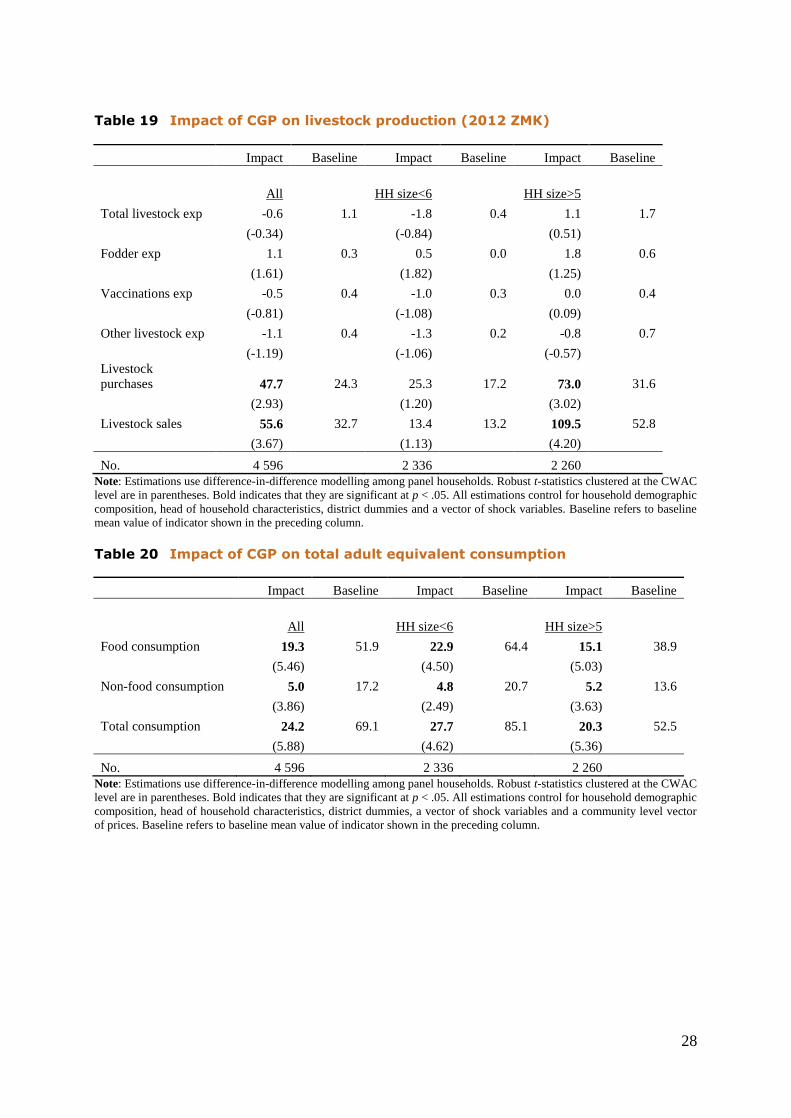
28

Table 19 Impact of CGP on livestock production (2012 ZMK)



Total livestock exp -0.6 1.1 -1.8 0.4 1.1 1.7

(-0.34) (-0.84) (0.51)

Fodder exp 1.1 0.3 0.5 0.0 1.8 0.6

(1.61) (1.82) (1.25)

Vaccinations exp -0.5 0.4 -1.0 0.3 0.0 0.4

(-0.81) (-1.08) (0.09)

Other livestock exp -1.1 0.4 -1.3 0.2 -0.8 0.7

(-1.19) (-1.06) (-0.57)

Livestock

purchases 47.7 24.3 25.3 17.2 73.0 31.6

(2.93) (1.20) (3.02)

Livestock sales 55.6 32.7 13.4 13.2 109.5 52.8

(3.67) (1.13) (4.20)

No. 4 596 2 336 2 260





Table 20 Impact of CGP on total adult equivalent consumption



Food consumption 19.3 51.9 22.9 64.4 15.1 38.9

(5.46) (4.50) (5.03)

Non-food consumption 5.0 17.2 4.8 20.7 5.2 13.6

(3.86) (2.49) (3.63)

Total consumption 24.2 69.1 27.7 85.1 20.3 52.5

(5.88) (4.62) (5.36)

No. 4 596 2 336 2 260



composition, head of household characteristics, district dummies, a vector of shock variables and a community level vector

of prices. Baseline refers to baseline mean value of indicator shown in the preceding column.

29

Table 21 Impact of CGP on type of food consumption



Share of households

Purchases -0.013 0.968 -0.018 0.964 -0.010 0.973

(-0.88) (-0.94) (-0.69)

Own produced 0.024 0.783 0.023 0.778 0.009 0.787

(0.60) (0.49) (0.20)

Gifts in kind -0.024 0.647 0.025 0.680 -0.064 0.613

(-0.54) (0.47) (-1.29)

Amount consumed per adult equivalent, ZMK

Purchases 16.0 22.7 18.2 28.1 13.8 17.0

(6.25) (4.96) (6.11)

Own produced 2.2 20.1 4.1 24.1 -0.4 16.1

(0.86) (1.19) (-0.20)

Gifts in kind 1.1 9.1 0.6 12.3 1.8 5.7

(0.92) (0.34) (1.85)

No. 4 596 2 336 2 260





Table 22 Impact of CGP on non-farm enterprise

Impact Follow-up Impact Follow-up Impact Follow-up

All HH Size<6 HH Size>5

HH operates NFE 0.166 0.390 0.157 0.390 0.177 0.380

(4.42) (3.6) (4.5)

Months in operation 1.445 2.830 1.201 2.800 1.629 2.850

(4.44) (3.38) (4.23)

Total monthly revenue (ZMK) 184.3 184.3 135.2 150.0 233.5 219.7

(4.43) (3.77) (3.65)

Total monthly profit (ZMK) 69.1 81.9 55.1 73.0 81.2 91.0

(4.05) (3.32) (3.78)

Owned business assets 0.045 0.120 0.024 0.130 0.067 0.120

(2.51) (1.04) (3.22)

Value of owned assets (ZMK) 196.6 134.6 17.2 46.6 342.0 225.1

(1.24) (0.66) (1.27)

No. 2 247 1 141 1106

Note: Estimations use single difference modelling among panel households. Robust t-statistics clustered at the CWAC level

are in parentheses. Bold indicates that they are significant at p < .05. All estimations control for household demographic



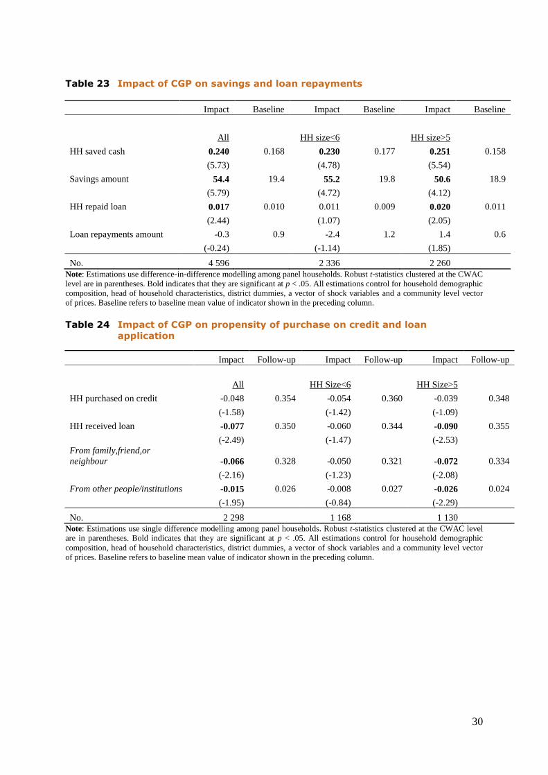
30

Table 23 Impact of CGP on savings and loan repayments



HH saved cash 0.240 0.168 0.230 0.177 0.251 0.158

(5.73) (4.78) (5.54)

Savings amount 54.4 19.4 55.2 19.8 50.6 18.9

(5.79) (4.72) (4.12)

HH repaid loan 0.017 0.010 0.011 0.009 0.020 0.011

(2.44) (1.07) (2.05)

Loan repayments amount -0.3 0.9 -2.4 1.2 1.4 0.6

(-0.24) (-1.14) (1.85)

No. 4 596 2 336 2 260





Table 24 Impact of CGP on propensity of purchase on credit and loan

application



HH purchased on credit -0.048 0.354 -0.054 0.360 -0.039 0.348

(-1.58) (-1.42) (-1.09)

HH received loan -0.077 0.350 -0.060 0.344 -0.090 0.355

(-2.49) (-1.47) (-2.53)

From family,friend,or

neighbour -0.066 0.328 -0.050 0.321 -0.072 0.334

(-2.16) (-1.23) (-2.08)

From other people/institutions -0.015 0.026 -0.008 0.027 -0.026 0.024

(-1.95) (-0.84) (-2.29)

No. 2 298 1 168 1 130





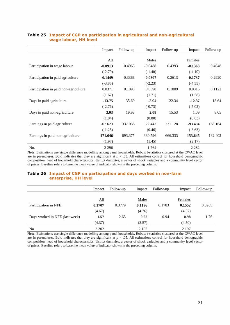
31

Table 25 Impact of CGP on participation in agricultural and non-agricultural

wage labour, HH level


All Males Females

Participation in wage labour -0.0913 0.4965 -0.0488 0.4393 -0.1363 0.4048

(-2.79) (-1.40) (-4.10)

Participation in paid agriculture -0.1449 0.3366 -0.0807 0.2613 -0.1737 0.2920

(-3.85) (-2.23) (-4.55)

Participation in paid non-agriculture 0.0371 0.1893 0.0398 0.1809 0.0316 0.1122

(1.67) (1.71) (1.58)

Days in paid agriculture -13.75 35.69 -3.04 22.34 -12.37 18.64

(-2.76) (-0.73) (-5.02)

Days in paid non-agriculture 3.03 19.93 2.08 15.53 1.09 8.05

(1.04) (0.80) (0.63)

Earnings in paid agriculture -67.623 337.038 22.443 221.128 -93.434 168.164

(-1.25) (0.46) (-3.63)

Earnings in paid non-agriculture 471.646 693.375 380.596 666.333 153.645 182.402

(1.97) (1.45) (2.17)

No. 2 296 1 764 2 282





Table 26 Impact of CGP on participation and days worked in non-farm

enterprise, HH level


All Males Females

Participation in NFE 0.1707 0.3779 0.1196 0.1783 0.1552 0.3265

(4.67) (4.76) (4.57)

Days worked in NFE (last week) 1.57 2.65 0.62 0.94 0.98 1.76

(4.37) (3.57) (4.50)

No. 2 202 2 102 2 197





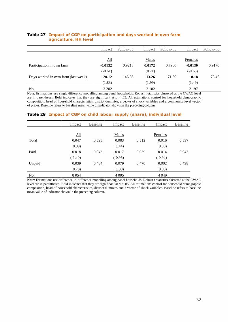
32

Table 27 Impact of CGP on participation and days worked in own farm

agriculture, HH level


All Males Females

Participation in own farm -0.0132 0.9218 0.0172 0.7900 -0.0139 0.9170

(-0.61) (0.71) (-0.65)

Days worked in own farm (last week) 20.12 146.66 13.26 71.60 8.18 78.45

(1.83) (1.99) (1.49)

No. 2 202 2 102 2 197





Table 28 Impact of CGP on child labour supply (share), individual level


All Males Females

Total 0.047 0.525 0.083 0.512 0.016 0.537

(0.99) (1.44) (0.30)

Paid -0.018 0.043 -0.017 0.039 -0.014 0.047

(-1.40) (-0.96) (-0.94)

Unpaid 0.039 0.484 0.079 0.470 0.002 0.498

(0.78) (1.30) (0.03)

No. 8 054 4 005 4 049





33

Table 29 Impact of CGP on the share household income sources



Crop production -0.032 0.342 -0.026 0.333 -0.035 0.352

(-0.97) (-0.72) (-1.03)

Livestock production 0.023 0.045 0.022 0.038 0.023 0.052

(3.08) (2.50) (1.92)

Fishing -0.003 0.024 -0.004 0.022 -0.002 0.026

(-0.37) (-0.45) (-0.19)

Non-farm enterprises 0.143 0.278 0.143 0.282 0.142 0.274

(4.18) (3.91) (3.80)

Wage employment -0.100 0.247 -0.103 0.257 -0.096 0.237

(-5.19) (-4.37) (-4.96)

Agricultural wage -0.101 0.159 -0.092 0.171 -0.106 0.148

(-5.26) (-4.06) (-5.14)

Non-agricultural wage 0.001 0.088 -0.011 0.086 0.010 0.089

(0.06) (-0.65) (0.80)

Transfers -0.031 0.064 -0.033 0.069 -0.032 0.059

(-3.62) (-3.32) (-3.09)

No. 2 282 1 157 1 125





34

Figures

Figure 1 Share of households producing each crop (over all households

producing crops), by district and treatment status (baseline)

0.2

.4.6

.81

0.2

.4.6

.81

Kaputa Kalabo Shang'ombo


control

treatment

Maize Cassava Rice Millet

Groundnut Sweet Potatoes Sorghum Other beans

Source: CGP Zambia

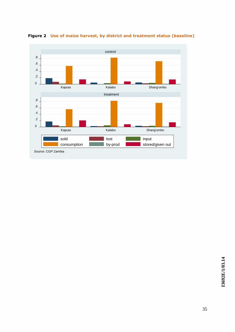
35

Figure 2 Use of maize harvest, by district and treatment status (baseline)

0

.2

.4

.6

.8

0

.2

.4

.6

.8



control

treatment

sold lost input

consumption by-prod stored/given out

Source: CGP Zambia

I3692E

/1/0

3.1

4

Date post:	20-Jun-2018
Category:	Documents
Upload:	doanhanh
View:	214 times
Download:	0 times

Zambia’s Child Grant Programme: 24-month impact report … · 24-month impact report on...

Documents