13–15 June 2013 Celje, Slovenia The International Conference on Logistics & Sustainable Transport 2013, website: http://iclst.fl.uni- mb.si/ A review of vehicular emission models Katja BAŠKOVIČ 1 and dr. Matjaž KNEZ 1 * 1 Faculty of logistics, University of Maribor, Celje, Slovenia Abstract—This paper reviews the latest literature about vehicular emission models. Vehicular emission models are methods for calculating the level of pollutant emissions, regarding emission factors, average speed, fuel consumption and the amount of traffic on the defined type of road. In the paper we are turning towards urban roads and looking for all types of vehicular emission models and good practice examples. Key words—emissions, practice examples, urban roads, vehicular emission models. I. INTRODUCTION All over the world we can see how the climate is changing. After few years when winters were almost snowless, we have snow from the end of October till the middle of the April, regardless we live in continental climate part of Slovenia. Temperatures can decrease from 12°C to –9°C over the night. Waters are flooding in larger areas than usual. Even if we look around the world, nowhere is better. Hurricanes and typhoons change the land, oceans level is rising and the Arctic sea ice is reaching its record melt. All presented facts are the consequence of the enhanced greenhouse effect, because human activities are releasing additional amounts of greenhouse gases (GHGs) into the atmosphere. The most commonly produced GHG is carbon dioxide (CO2). Since the Industrial Revolution the concentration of CO2 in the atmosphere has increased by around 41% and it rises. One of the main sources of CO2 is the combustion of fossil fuels to power machines, generate electricity, heat buildings and above all to transport people and goods. Other GHGs are emitted in smaller quantities than CO2, but they trap heat far more effectively [1]. Transport is responsible for around a quarter of EU GHG emissions. As can be seen from Fig. 1, this makes it the second biggest GHG emitting sector after energy. While emissions from other sectors are generally falling, those from transport have increased 36% between 1990 and 2007. The EU has policies in place to reduce emissions from a range of modes of transport, such as including aviation in the EU Emissions Trading System (EU ETS) and CO2 emissions targets for cars [2]. Figure 1: EU27 greenhouse gas emissions by sector and mode of transport, 2007 [3].
Transcript
13–15 June 2013 Celje, Slovenia
The International Conference on Logistics & Sustainable Transport 2013, website: http://iclst.fl.uni-mb.si/
A review of vehicular emission models Katja BAŠKOVIČ1 and dr. Matjaž KNEZ1*
1 Faculty of logistics, University of Maribor, Celje, Slovenia
Abstract—This paper reviews the latest literature about vehicular emission models. Vehicular emission models
are methods for calculating the level of pollutant emissions, regarding emission factors, average speed, fuel
consumption and the amount of traffic on the defined type of road. In the paper we are turning towards urban
roads and looking for all types of vehicular emission models and good practice examples.
Key words—emissions, practice examples, urban roads, vehicular emission models.
I. INTRODUCTION
All over the world we can see how the climate is changing. After few years when winters were almost snowless, we have snow from the end of October till the middle of the April, regardless we live in continental climate part of Slovenia. Temperatures can decrease from 12°C to –9°C over the night. Waters are flooding in larger areas than usual. Even if we look around the world, nowhere is better. Hurricanes and typhoons change the land, oceans level is rising and the Arctic sea ice is reaching its record melt.
All presented facts are the consequence of the enhanced greenhouse effect, because human activities are releasing additional amounts of greenhouse gases (GHGs) into the atmosphere. The most commonly produced GHG is carbon dioxide (CO2). Since the Industrial Revolution the concentration of CO2 in the atmosphere has increased by around 41% and it rises. One of the main sources of CO2 is the combustion of fossil fuels to power machines, generate electricity, heat buildings and above all to transport people and goods. Other GHGs are emitted in smaller quantities than CO2, but they trap heat far more effectively [1].
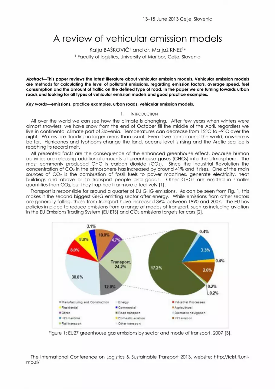
Transport is responsible for around a quarter of EU GHG emissions. As can be seen from Fig. 1, this makes it the second biggest GHG emitting sector after energy. While emissions from other sectors are generally falling, those from transport have increased 36% between 1990 and 2007. The EU has policies in place to reduce emissions from a range of modes of transport, such as including aviation in the EU Emissions Trading System (EU ETS) and CO2 emissions targets for cars [2].
Figure 1: EU27 greenhouse gas emissions by sector and mode of transport, 2007 [3].
13–15 June 2013 Celje, Slovenia
The International Conference on Logistics & Sustainable Transport 2013, website: http://iclst.fl.uni-mb.si/
Road transport contributes about one-fifth of the EU's total emissions of CO2. Its emissions from road transport increased by nearly 23% between 1990 and 2010, and without the economic downturn growth could have been even bigger [4].
Other pollutant emissions emitting in road transport are carbon monoxide (CO), sulfur dioxide (SO2), lead, hydrocarbons (HC), oxides of nitrogen (NOx), non-methane volatile compounds (NMVOC) and particulate matter (PM).
European Commission (EC) implements different strategy following regulations on reducing CO2 and other pollutant emissions from vehicles. Their reduction target is under the Kyoto Protocol and beyond [4].
There are many possibilities how to measure, calculate and control the pollutant emission. From many possibilities we peak emission models which are very useful to calculate and show the amount of emissions in selected area.
In the following chapter can be seen the descriptions of all covered emission models classified in different groups and the descriptions of selected, after 2002 presented, vehicular emission models.
II. VEHICULAR EMISSION MODELS
Vehicular emission models are methods for calculating the level of pollutant emissions, regarding emission factors, average speed, fuel consumption and the amount of traffic on the defined type of road.
There are two different arrangements of vehicular emission models. In reference [5] emission models are primary classified on modelling approaches used when calculating hot, cold start and evaporative emissions. Secondary hot emission models are classified into three main groups of increasing level of complexity:
(a) emission factor models,
(b) average speed models,
(c) modal emission models.
In reference [6] emission models are classified according to the input data, the scale of the study and the type of pollutants being considered:
(a) model relying on fuel quantities,
(b) model relying on average traffic volumes per detailed categories of vehicles,
(c) model relying on average speed of the traffic,
(d) model implying detailed description of traffic situation,
(e) model providing the emissions from traffic related variable,
(f) model representing a detailed description of speeds experienced,
(g) model relying on chronological speed (instantaneous model).
A. Emission model groups descriptions
Groups from both classifications can be combined in one list of groups and subgroups. How are they connected can be seen from their following description.
1) Emission factor model
Emission factor models function with a simple calculation method and do not require large amounts of input data. The estimation of the emissions is expressed by the use of an emissions factor related to one type of vehicle and a specific driving mode (i.e. urban, rural or motorway). Emission factors are derived from the mean values of repeated measurements over a particular driving cycle and are usually expressed in mass of pollutant per unit distance. Emission factor models are commonly used in the development of national and regional emission inventories. This approach is not accurate on microscale, regarding the emission factors are based on average driving characteristics [5].
2) Average speed model
Average speed models are based on speed-related emission functions, generated by the measurements of the emission rates over a variety of trips at different speed levels. These models are often used in emission inventories on a road network scale. Their use on a microscale level is inappropriate, because they usually do not include changes in operational modes [5].
13–15 June 2013 Celje, Slovenia
The International Conference on Logistics & Sustainable Transport 2013, website: http://iclst.fl.uni-mb.si/
3) Modal emission model
Modal emission models operate at a higher level of complexity. Modal models based on speed and acceleration present the emission rates as a function of different levels of speed as well as of the various operational modes (i.e. acceleration, deceleration, steadly-speed cruise and idle). They provide more accurate emissions estimation at a microscale level than emission factor and average speed models. Modal models based on speed and acceleration can be specific enough to provide emission levels or fuel consumption, second-by-second, for a particular type of vehicle from a given driving cycle.
Modal models based on engine power present emissions as a function of engine demand and other physical parameters related to vehicle operation. This type of model is usually highly complex due to the large amount of data required [5].
4) Model relying on fuel quantities
Models use fuel consumption data (i.e., fuel sale data) and categories of vehicles. Models can only be used for large-scale inventories [6].
5) Model relying on average traffic volumes per detailed categories of vehicles
Models use a single emission factor to represent a particular type of vehicle and driving cycle. The emission factors are calculated as mean values of measurements on a number of vehicles over given driving cycles, and are usually stated in terms of the mass of pollutant emitted per vehicle distance of fuel. These factors are mostly used in national and regional emission inventories [6].
6) Model relying on average speed of the traffic
These models predict average emission factors for a vehicle class that is driven over a number of different driving patterns, which are a function of the mean travelling speed. The total emissions can be calculated by the sum of the exhaust emissions (hot and cold), evaporative emissions and for some models emissions due to road vehicle tires and brakes as well as road wear resulting from the vehicles’ motion. The results of these models may not be very precise, but they cover the major emission processes and most pollutants of interest [6].
7) Model implying detailed description of traffic situation
These models use discrete emission factors for predefined traffic situations (e.g. stop-and-go, saturated, heavy, free flow). They allow the estimation of pollutants emitted by the hot and cold exhaust emissions as well as fuel evaporation. The methodologies were also developed for small scales (i.e. single street). Traffic situation models require vehicle-kilometre-travelled (VKT) data per driving situation as input. These models provide emissions for a large number of different regulated and non-regulated pollutants [6].
8) Model providing the emissions from traffic related variable
Emission factors obtained from traffic-variable models are defined by traffic flow variables such as average speed, traffic density, queen length and signal settings. They use a correction of the average speed to assume the effects of the traffic onto pollutant emissions [6].
9) Model representing a detailed description of speeds experienced
These models are based on tests on a large number of vehicles according to various driving cycles. Within the model, each driving cycle is characterized by a large number of descriptive parameters (e.g. average speed, number of stops per km, kinematics of vehicles). For each pollutant and vehicle category, a regression model is fitted to the average emission values over the different driving cycles. These models require detailed information on the movement of the vehicles (instantaneous speed, acceleration) [6].
10) Model relying on chronological speed (instantaneous model)
These models represent explicitly the vehicle emission behaviour by relating emission rates to vehicle operation during series of short time steps. In some models, vehicle operation is defined in terms of a relatively small number of modes (i.e. idle, acceleration, deceleration and cruise). For
13–15 June 2013 Celje, Slovenia
The International Conference on Logistics & Sustainable Transport 2013, website: http://iclst.fl.uni-mb.si/
each of the modes, the emission rate for a given vehicle category and pollutant is fixed and the total emission rate is calculated by weighting each model emission rate by the time spent in each mode. Some instantaneous models relate vehicle engine power, speed and acceleration during a driving cycle. The model estimates only hot running emissions [6].
B. List of groups and subgroups
Regarding presented descriptions we combined all groups in the following list:
Emission factor model
o Model relying on fuel quantities,
o Model relying on average traffic volumes per detailed categories of vehicles.
Average speed model
o Model relying on average speed of the traffic.
Modal emission model
o Model implying detailed description of traffic situation,
o Model providing the emissions from traffic related variable,
o Model representing a detailed description of speeds experienced,
o Model relying on chronological speed (instantaneous model).
C. Description of vehicular emission models
In the following paragraphs examples of new, after 2002 presented, vehicular emission models are described.
1) Microscale Emission Model POLY
Microscale emission models [7] were developed due to the difficulty of presenting acceleration or deceleration in a macroscale emission model. These models can estimate second-by-second emissions.
Microscale emission models ei,j,k,m(t) where developed for each emission type m (e.g. CO, HC or NOx) and light-duty vehicle categories (vehicle size (i), model year (j), emitter type (k)) by adopting least-square regression. The proportion Pi,j,k for each category (i, j, k) was derived based on the national level of vehicle distributions.
The emission of type m, that is produced by a vehicle with size i at time t, ei,m(t) can be estimated as
(1)
Vehicles were classified into categories by size: light-duty gasoline vehicle (LDGV) (i.e., passenger cars), light-duty gasoline trucks under 6,000 lbs. gross vehicle weight (LDGT1) and light-duty gasoline trucks 6,000 lbs. to 8,500 lbs. gross vehicle weight (LDGT2); by model year (e.g. before 1975, 1975-1980, 1981-1986, 1987-1990, 1991-1993, 1994-1997 for LDGV) and into five different emitter type groups: one normal emitter and four high-emitter types. Result of classification is 41 groups of vehicles made before 1997.
The type m emission rate (g/s) for vehicle group (i, j, k) at time t, ei,j,k,m(t)in modelling is represented as
(2)
where three factors were taken into account: tractive power, grade and time dependence. Tractive power is represented by using variables W(t), V(t), V2(t) and V3(t). W(t) is related to kinetic power, which is a part of tractive power:
(3)
where M is the vehicle mass with appropriate inertial correction for rotating and reciprocating parts (kg); g0=gravitational constant (9.81 m/s); φ is the grade of roadway; and a(t)is the acceleration or deceleration rate at time t.
The effect of grade of a roadway, A(t) (i.e. combined acceleration or deceleration rate) is formulated as
(4)
13–15 June 2013 Celje, Slovenia
The International Conference on Logistics & Sustainable Transport 2013, website: http://iclst.fl.uni-mb.si/
where a(t) is a vehicle’s actual acceleration or deceleration rate; and g(t) represents the grade (percentage) of the roadway segment where a vehicle is travelling at time t.
Time dependence in emissions response to vehicle operation (e.g. the use of timer to delay command enrichment or oxygen storage in the catalytic converter) was taken into account in this project by employing time-series variables. Researcher figured out that the acceleration or deceleration in the preceding time periods, not in current time, has the most obvious impact on the emissions at time t. Patterns of impact are not the same for different emission types. To consider the impact in model variables of combined accelerations or decelerations rates in the current and past periods (i.e. A(t),…,A(t-9)) were used.
There are also two variables used in (2), T’(t) to represent the duration of acceleration and T’’(t) to represent the duration of deceleration. At specific point in time, only one value can be greater than zero.
The emission model (2) was validated through the root mean squared error (RMSE), the aggregated total prediction error (ATPE) and the correlation coefficient (R) between the predicted and actual emissions. Model POLY (1) was compared with the model CMEM and the emissions model Integration that was adopted in the microscopic traffic simulation model. Because the emission models developed in this project were based on the data set of the Federal Test Procedure (FTP) cycle, researchers used second-by-second emissions data of the modal emission cycle (MEC) and the US06 cycle. From results of comparisons through the RMSEs, ATPEs and correlation coefficient it can be observed that the POLY models has the same trend of change as the measured emissions and predicts more accurately than the other two models most of the time.
2) Microscale Emission Factor Model for Particulate Matter (MicroFacPM)
A microscale emission factor model for PM (MicroFacPM) [8] for predicting real-world real-time motor vehicle emissions for total suspended PM (TSP), PM less than 10μm aerodynamic diameter (PM10) and PM less than 2.5μm aerodynamic diameter (PM2.5) has been developed to support studies about human exposure near roadways and inside vehicles travelling along the roadways. The research was funded by Environmental Protection Agency (EPA).
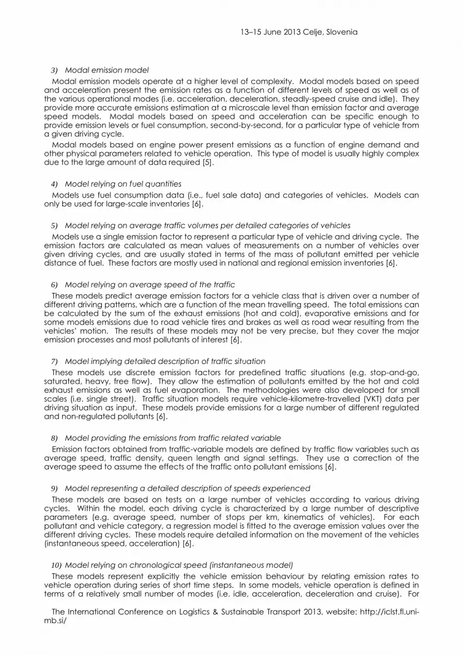
The model is written in FORTRAN 90 for calculating emission factors from vehicular traffic in United States. It uses modelling concepts and structure similar that is used in the development of a microscale emission factor model for CO (MicroFacCO). MicroFacPM uses available information concerning the vehicle fleet composition. General models structure of the MicroFacPM can be seen from Fig. 2.
Figure 2: The MicroFacPM general model structure
13–15 June 2013 Celje, Slovenia
The International Conference on Logistics & Sustainable Transport 2013, website: http://iclst.fl.uni-mb.si/
The emission factors are calculated from a real-time fleet. MicroFacPM requires many input variables for each specific time interval: job title, number of roads, date, time, smoking vehicle percentage, ambient temperature, relative humidity, vehicle fleet type, output option, roadway type, number of lanes (maximum is eight lanes, possibility of parallel road networks modelling) and average vehicle speed. Similar to MicroFacCo, MicroFacPM has seven options for inputting the vehicle fleet characterization. The model can accept input based on a detailed observed vehicle fleet (options 1 and 2), past vehicle tunnel data (options 3 and 4), video records (options 5 and 6) or a default vehicle fleet (option 7).
The model output can be obtained in three categories: option 1 outputs detailed information on the correction factors for each vehicle type and model year; option 2 outputs the proportion of PM per vehicle type, model year and source; and option 3 outputs lane-by-lane composite emission rates for the fleet.
The motor vehicle fleet is divided into two main categories: light-duty vehicles (i.e. vehicles with gross vehicle weight (GVW) ratings less than 8,500 lb) and heavy-duty vehicles (i.e. vehicles with GVW ratings more than 8,500 lb). Further, those two categories together are divided into 31 classes.
Light-duty vehicle particulate emission rates are calculated in mg/mi by testing a vehicle over a standardized test cycle known as Urban Dynamometer Driving Schedule (UDDS) on a chassis dynamometer. UDDS is part of EPA’s FTP, which is used by all motor vehicle manufacturers to certify that their vehicles meet federal tailpipe emission standards. MicroFac models use UDDS phase 1 for cold running emission rate and phases 2 and 3 for hot running emission rates (hot running emission rate = 0.521 * phase 2 emission rate + 0.479 * phase 3 emission rate). Tests were made on gasoline and on diesel light-duty vehicles.
Heavy-duty vehicles testing to determine PM emission rates is performed either on chassis dynamometers (similar to testing light-duty vehicles) or on engine dynamometers. In case of the method with engine dynamometers emission rates are determined in grams per brake-horsepower-hour (g/bhp-hr) by testing the engine over a heavy-duty transient test (HDTT) cycle. The emission rates in mg/mi are estimated by multiplying emission rates in mg/bhp-hr by a conversion factor in bhp-hr/mi. Tests were made on gasoline and on diesel heavy-duty vehicles.
Accounting non-exhaust emission rates MicroFacPM uses averaged break-wear and tire-wear emission rates for cars, measured on breaking cycles representative of urban driving, because of the limited testing for all types of vehicle. Averaged break-wear particulate emission rate is 0.0128 g/mi and averaged air borne tire-wear particulate emission rate is 0.002 g/mi. To obtain tire-wear emission rates from the vehicle, the tire emission is multiplied by the number of wheels on the vehicle.
MicroFacPM fully accounts for the distance travelled by vehicles during a cold-start operating mode in calculating the composite emission rates. The MicroFacPM cold-start function goes to zero effect after a few miles, depending upon ambient temperature. Cold mileage percentage (CPM) for a model year is calculated as:
(5)
where CPMi,j is the cold mileage percentage for vehicle type i and model year j, TC is the ambient air temperature (°C) and ltripi,j is the length of the trip (mi) for vehicle type i and model year j. In MicroFacPM, the effect of cold mileage percentage is considered only for light-duty vehicles with gasoline engines, all other vehicles are assumed to be running with hot engines.
The UDDS driving cycle measures emission rates at an average speed of 19.6 mi/hr, therefore, emission rates have to be corrected for on-road average speeds. The following correction factors are used in the model for light heavy-duty diesel vehicles (i.e. diesel vehicles with GVW between 8,501 lb and14,000 lb): 1.0 (V ≤ 12.5 mi/hr); –0.0321*V + 1.4013 (V = 12.5 to 25.0 mi/hr); –0.0053*V + 0.7303 (V > 25.0 to 50.0 mi/hr); 0.47 (V > 50.0 mi/hr).
MicroFacPM accounts for the exhaust emission factors resulting from air-conditioning operations based on their fuel consumption for light-duty gasoline vehicles and trucks.
The MicroFacPM composite emission rate for the vehicle fleet is calculated by incorporating all previously described parameters:
(6)
13–15 June 2013 Celje, Slovenia
The International Conference on Logistics & Sustainable Transport 2013, website: http://iclst.fl.uni-mb.si/
where ERi,j is the composite emission rate for vehicle type i and model year j, NERi,j is the normal emission rate for vehicle type i and model year j, BERi,j is the non-normal emission rate for vehicle type i and model year j, ColdTi,j is the temperature correction factor for the cold operating mode for vehicle type i and model year j, CMPi,j is the cold mileage percentage for vehicle type i and model year j, fail is the percentage of smoking (non-normal emitting) vehicles, ACi is the air conditioning correction factor for vehicle type i, ACVi,j is the fraction of vehicles with air conditioning for vehicle type i and model year j and Vi is the speed correction factor for vehicle type i.
These emission rates (mg/mi) are than multiplied by the fraction of vehicles of each model year and vehicle class to get the proportions of emissions:
(7)
where CEFi,j is the proportion of composite emission factor for vehicle type i and model year j and VEHi,j is the fraction of vehicles for vehicle type i and model year j.
The composite emission factor for the entire fleet is calculated as:
(8)
This models captures virtually all the real-world information for the U.S. motor vehicle fleet.
3) Model REPAS
Model REPAS [9] calculates the CO2 emission from passenger cars (PC), taking into account certain specific features proper to transition countries with older vehicles fleet. The model was implemented on PC fleet in Montenegro.
Based on this model, software REPAS 1.1 was developed, for calculation of total emission of CO2
and also specific emission of CO2 from PCs registered in Montenegro in 2003. The software includes data for fuel use according to manufacturer declaration for 1,620 vehicle types by various manufacturers, proper to the territory of Montenegro.
Model REPAS predicts the reduction of the emitted CO2 volume due to incomplete combustion, inefficiency of the system for after-treatment of exhaust gases and a number of other parameters causing reduction. Totally emitted CO2 per year (ECO2) from PC is determined as:
(9)
where are: i = number of vehicle categories (i=1, …, 32); Ni = number of registered vehicles in the observed category i [vehicles/year]; li = average annual mileage of category i [km/vehicles, year]; j = number of types per category i (j=1, …, m); gECEj = manufacturer ECE test specific fuel consumption of PC model j of category i [liters of fuel/100 km]; rj = share of type j in category i; KgECEi = worsening degree of the manufacturer-indicated fuel consumption of vehicles category i; Kzi = emission factor of vehicles category i [kg CO2/liters of fuel]; and Knsj = incomplete combustion coefficient of vehicles category i.
Emission factor of CO2 (Kz) is determined as:
(10)
where eCO2 is specific emission of CO2 [gCO2/km] and G is specific fuel consumption [lfuel/100 km].
Correction coefficient of incomplete combustion Kns is necessary to take into account, because the engine operating in the area of rich mixture creates high concentration of incomplete combustion products such as CO and HC, and low concentration of CO2. It is determined as:
(11)
where CO2 is measured concentration of CO2 in the exhaust gases of motor vehicles from the observed category, and CO2F is manufacturer test data for the concentration of CO2 in the exhaust gases of motor vehicles for individual models.
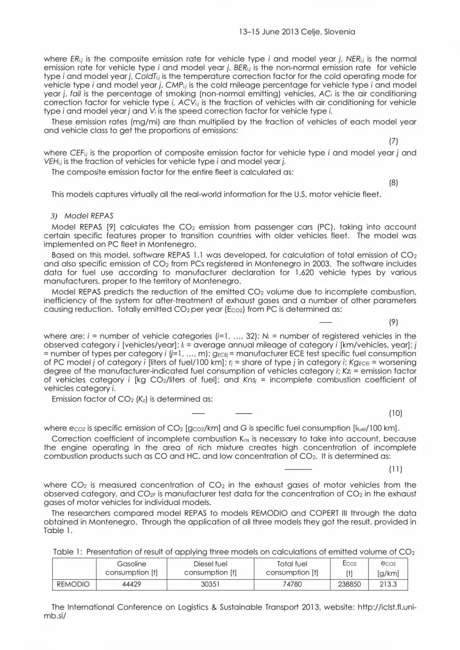
The researchers compared model REPAS to models REMODIO and COPERT III through the data obtained in Montenegro. Through the application of all three models they got the result, provided in Table 1.
Table 1: Presentation of result of applying three models on calculations of emitted volume of CO2
Gasoline
consumption [t]
Diesel fuel
consumption [t]
Total fuel
consumption [t]
ECO2
[t]
eCO2
[g/km]
REMODIO 44429 30351 74780 238850 213.3
13–15 June 2013 Celje, Slovenia
The International Conference on Logistics & Sustainable Transport 2013, website: http://iclst.fl.uni-mb.si/
COPERT III 37577 27302 64879 205283 183.3
REPAS 44171 30924 75095 186990 167
As can be seen from Table 1, models REPAS and REMODIO are comparable in fuel consumption. Model COPERT III, which was developed for needs of European Union (EU), calculated much lower volume of leaded fuel consumption; the leaded fuel was being that time already phased out from the EU.
The results of calculating ECO2 obtained by applying the model REPAS show the lowest values. Values by the other two models are higher for 10% (i.e. by COPERT III) and 28% (i.e. by REMODIO).
From the comparison results researchers concluded that the anomaly of reducing the concentration of CO2 in the exhaust gases of motor vehicle in use was proven and presented through model REPAS.
4) An Intelligent Agent Mobile Emissions Model
An intelligent agent mobile emission model [10] is a microscopic mobile emissions model based on an intelligent agent model of vehicles. Researchers’ development based on Multi-Agent System, where vehicles are designed as intelligent agents, and every agent is capable of representing the characteristics of an individual driver.
Researchers presumed that the model is the core of every agent and that the agent (vehicle) n follows the agent n – 1. This model includes drivers’ characteristics based on the full speed difference model. It is determined as:
, (12a)
, (12b)
, (12c)
, (12d)
where x is the vehicle position; v is the vehicle speed; t is the time; n is the vehicle sequence; ∆xn = x(n-
1) – xn; ∆vn = v(n-1) – vn; i is the type of driver (i = 1, …, m); q(i) is the character of the i-type driver (i.e. the degree of acceleration); Pc(i) is the probability of all kinds of drivers ( ); and k, λ, v1, v2, C1, C2, and lc are coefficients. The model is called the Intelligent Agent Car-Following (IACF) model, because the simulated vehicles in this model function as a simple intelligent agent system.
The most important factor affecting urban mobile emissions is the functional status of each vehicle, including speed, acceleration and rotational speed. Vehicle’s speed, acceleration and emissions are expressed as:
(13)
where E represents mobile emissions; a is the acceleration; v is the speed; and e, b, c, and d are coefficients. According to (13), mobile emissions can be calculating using the speed and acceleration of vehicles.
The speed and acceleration are input variables in micro-mobile emissions model and output variables in the proposed vehicle intelligent agent model. From these models, i.e., (12a), (12b), (12c), (12d) and (13), researchers developed a hybrid microcosmic mobile emissions model determined as:
(14)
where En(t) represents mobile emissions (mg/s), which denotes HC, CO, and NOx; e, b, c, d, k, λ, v1, v2, C1, C2, and lc are coefficients that must be identified using actual experimental data; and a is the acceleration (m/s2).
13–15 June 2013 Celje, Slovenia
The International Conference on Logistics & Sustainable Transport 2013, website: http://iclst.fl.uni-mb.si/
Researchers tested the model through a vehicle driving simulator. A total of 128 testees have driven and followed a vehicle in the simulator for 150 seconds. Their operation, speed and acceleration were recorded and the statistical data were analyzed. Through many experiments and examinations the model coefficients were identified. Speed and acceleration are the combining parameters for integration of micro-flow traffic models, where speed and acceleration are calculated, in micro-mobile emission models, where speed and acceleration are applied.
The case study revealed that HC, CO, and NOx emissions differ during a vehicle’s functioning process based on individual driver characteristics (e.g. the reckless drivers generate more emissions.
5) VT-Meso model
VT-Meso model [11] is a mesoscopic model that estimates vehicle fuel consumption and emission rates using a limited number of easily measurable input parameters, i.e., the average trip speed, number of stops per unit distance and average stop duration. The model is developed from data constructed using VT-Micro model to ensure consistency across the various modelling approaches. Researchers wanted to develop a model that is sensitive to various modes of vehicle operation but does not require detailed second-by-second vehicle speed and acceleration measurements. This model provides a compromise between model efficiency and model applicability.
The model is primarily intended for use after the traffic demand has been predicted and assigned to the network to estimate link-by-link input parameters, which are utilized to construct synthetic drive cycle and compute average link fuel consumption and emission rates. A synthetic drive cycle produces consistent average speed, number of vehicle stops and stop delay estimates. After constructing the drive cycle, the model estimates the proportion of time that a vehicle typically spends cruising, decelerating, idling and accelerating by travelling on a link. A series of fuel consumption and emission models are than used to estimate the amount of fuel consumed and emissions of HC, CO, CO2 and NOx for each mode of operation. To obtain distance-based average vehicle fuel consumption and emission rates, the total fuel consumed and pollutants emitted by a vehicle while travelling along a segment are estimated by summing across the different modes of operation and dividing by the distance travelled. Schematic of model procedure can be seen from Fig. 3.
Figure 3: Schematic of mesoscopic model
The model is based on the principle that the vehicle acceleration is proportional to the resulting force applied to it:
(15)
13–15 June 2013 Celje, Slovenia
The International Conference on Logistics & Sustainable Transport 2013, website: http://iclst.fl.uni-mb.si/
where a is the instantaneous acceleration (m/s2); F is the residual tractive force (N); R is the total resistance force (N); M is the vehicle mass (kg); and α is the fraction of the maximum acceleration that is utilized by the driver.
Tractive force F is computed at any given speed as:
(16a)
(16b)
(16c)
where Ft is the tractive force applied on vehicle (N); Fmax is the maximum attainable tractive force (N); P is the maximum engine power (kW); η is the engine efficiency; v is the vehicle speed (km/h); pmta is the portion of vehicle mass on the tractive axle; M is the mass of the vehicle; and μ is the coefficient of friction between the vehicle tires and roadway pavement.
External resistance force R is calculated as:
(17a)
(17b)
(17c)
(17d)
where Ra is the aerodynamic resistance (N); Rr is the rolling resistance (N); Rg is the grade resistance (N); A is the frontal area of the vehicle(m2); H is the altitude (m); Cd is the air drag coefficient; Ch is the altitude coefficient (Ch=1–0.000085H); v is the speed (m/s); Cr, c2, and c3 are the rolling resistance constants; M is the mass of the vehicle (kg); and i is the roadway grade (m/100m).
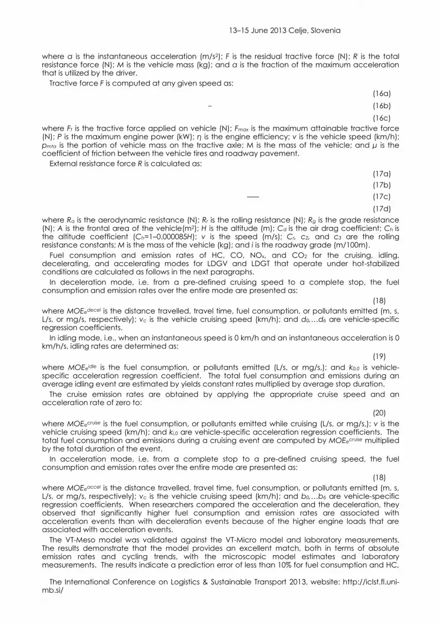
Fuel consumption and emission rates of HC, CO, NOx, and CO2 for the cruising, idling, decelerating, and accelerating modes for LDGV and LDGT that operate under hot-stabilized conditions are calculated as follows in the next paragraphs.
In deceleration mode, i.e. from a pre-defined cruising speed to a complete stop, the fuel consumption and emission rates over the entire mode are presented as:
(18)
where MOEedecel is the distance travelled, travel time, fuel consumption, or pollutants emitted (m, s, L/s, or mg/s, respectively); vc is the vehicle cruising speed (km/h); and d0,…d6 are vehicle-specific regression coefficients.
In idling mode, i.e., when an instantaneous speed is 0 km/h and an instantaneous acceleration is 0 km/h/s, idling rates are determined as:
(19)
where MOEeidle is the fuel consumption, or pollutants emitted (L/s, or mg/s,); and k0,0 is vehicle-specific acceleration regression coefficient. The total fuel consumption and emissions during an average idling event are estimated by yields constant rates multiplied by average stop duration.
The cruise emission rates are obtained by applying the appropriate cruise speed and an acceleration rate of zero to:
(20)
where MOEecruise is the fuel consumption, or pollutants emitted while cruising (L/s, or mg/s,); v is the vehicle cruising speed (km/h); and ki,0 are vehicle-specific acceleration regression coefficients. The total fuel consumption and emissions during a cruising event are computed by MOEecruise multiplied by the total duration of the event.
In acceleration mode, i.e. from a complete stop to a pre-defined cruising speed, the fuel consumption and emission rates over the entire mode are presented as:
(18)
where MOEeaccel is the distance travelled, travel time, fuel consumption, or pollutants emitted (m, s, L/s, or mg/s, respectively); vc is the vehicle cruising speed (km/h); and b0,…b6 are vehicle-specific regression coefficients. When researchers compared the acceleration and the deceleration, they observed that significantly higher fuel consumption and emission rates are associated with acceleration events than with deceleration events because of the higher engine loads that are associated with acceleration events.
The VT-Meso model was validated against the VT-Micro model and laboratory measurements. The results demonstrate that the model provides an excellent match, both in terms of absolute emission rates and cycling trends, with the microscopic model estimates and laboratory measurements. The results indicate a prediction error of less than 10% for fuel consumption and HC,
13–15 June 2013 Celje, Slovenia
The International Conference on Logistics & Sustainable Transport 2013, website: http://iclst.fl.uni-mb.si/
CO, and CO2 emission rates, with higher prediction errors in the case of NOx emissions (10 to up to 27% error.
III. CONCLUSIONS
The paper reviews the latest literature about vehicular emission models. There are two different classifications of vehicular emission models. After seeing their descriptions, they have been combined into one list: emission factor models: models relying on fuel quantities, models relying on average traffic volumes per detailed categories of vehicles; average speed models: model relying on average speed of the traffic; modal emission models: models implying detailed description of traffic situation, models providing the emissions from traffic related variable, models representing a detailed description of speeds experienced, models relying on chronological speed (instantaneous models).
In the latest years there have been many developments on this field. In this paper described models were chosen, because they were presented after 2002, when another review of vehicular emission models was published [5], and they are something new in the development of models this kind. Chosen models are: Microscale Emission Model POLY, which was developed to present the impact of acceleration and deceleration in emission emitting; MicroFacPM, which was developed to support studies about human exposure near roadways and inside vehicles travelling along the roadways; Model REPAS, which was developed to take into account certain specific features proper to transition countries with older vehicles fleet; An Intelligent Agent Mobile Emissions Model, which was developed to take into account the characteristics of an individual driver; and VT-Meso model, which was developed to provide a compromise between model efficiency and model applicability.
These models have all contributed something new to vehicular emission models: different accession to modelling acceleration and non-exhaust emission rates, representation of the anomaly of reducing the concentration of CO2, accounting drivers’ characteristics in acceleration modelling, and also generalization of drive cycle into synthetic drive cycle.
It has been observed that lately mostly modal models are developed. None the less, modal models should also account the impact of cold start and drivers’ characteristic, where possible, enhancement to all sorts of fuel and types of vehicles. In majority acceleration is accounted, not always in the connection with grade of roadway, which also has an important impact on emission emitting.
REFERENCES
1. EC, “What's causing the climate change?” 10th September 2012 [Accessed 2nd April 2013 on URL: http://ec.europa.eu/clima/policies/brief/causes/index_en.htm#other_ghg].
2. EC, “Reducing emissions from transport,” 6th Januar 2011 [Accessed 5th April 2013 on URL: http://ec.europa.eu/clima/policies/transport/index_en.htm].
3. EU Transport GHG: Routes to 2050, “The contribution of transport to GHG emissions,” 21th March 2011 [Accessed 6th April 2013 on URL: http://www.eutransportghg2050.eu/cms/the-contribution-of-transport-to-ghg-emissions/].
4. EC, “Road transport: Reducing CO2 emissions from vehicles,” 30th July 2012 [Accessed 5th April 2013 on URL: http://ec.europa.eu/clima/policies/transport/vehicles/index_en.htm].
5. A. Esteves-Booth, T. Muneer, J. Kubie and H. Kirby, “A review of vehicular emission models and driving cycles,” Proceedings of the Institution of Mechanical Engineers, Part C: Journal of Mechanical Engineering Science, vol. 216, August 2002, pp. 777-797.
6. M. Fallahshorshani, M. André, C. Bonhomme and C. Seigneur, “Coupling Traffic, Pollutant Emission, Air and Water Quality Models: Technical Review and Perspectives,” Procedia - Social and Behavioral Sciences, vol. 48, 2012, pp. 1794-1804.
7. Y. G. Qi, H. H. Teng and L. Yu, “Microscale Emission Models Incorporating Acceleration and Deceleration,” Journal of Transportation Engineering, vol. 130, no. 3, May 2004, pp. 348-359.
8. R. B Singh, A. H. Huber and J. N. Braddock, “Development of a Microscale Emission Factor Model for Particulate Matter for Predicting Real-Time Moor Vehicle Emissions,” Journal of the Air & Waste Management Association, vol. 53, October 2003, pp. 1204-1217.
9. R. Vujadinović and D. Nikolić, “Innoated Model REPAS for Calculation of CO2 Emission from Passenger Cars in Developing Countries,” in EnviroInfo 2007, O. Hryniewicz, J. Studzinski, M. Romaniuk, A. Szediw, Eds. Warsaw: Shaker Verlag, pp. 229-237.
10. C. Z. Wu, X. P. Yan, G. H. Huang and Y. P. Li, “An Intelligent Agent Mobile Emissions Model for Urban Environmental Management,” International Journal of Software Engineering and Knowledge Engineering, Vol. 18, No. 4, 2008, pp. 485-502.
11. H. Rakha, H. Yue and F. Dion, “VT-Meso model framework for estimating hot-stabilized light-duty vehicle fuel consumption and emission rates,” Canadian Journal of Civil Engineering, vol. 38, 2011, pp. 1274-1286.
13–15 June 2013 Celje, Slovenia
The International Conference on Logistics & Sustainable Transport 2013, website: http://iclst.fl.uni-mb.si/
AUTHORS
Baskovic K., is a student at the University of Maribor, Faculty of Logistics, Mariborska cesta 7, 3000 Celje, Slovenia (e-mail: [email protected]).
Knez M., is with University of Maribor, Faculty of Logistics, Mariborska cesta 7, 3000 Celje, Slovenia (e-mail: [email protected]).
Manuscript received by 1 May 2013. [Submitted 1 May 2013.]