Author's personal copy Nannofossil biostratigraphy, strontium and carbon isotope stratigraphy,...

Author's personal copy

Nannofossil biostratigraphy, strontium and carbon isotope stratigraphy,cyclostratigraphy and an astronomically calibrated duration of the LateCampanian Radotruncana calcarata Zone

Michael Wagreich a,*, Johann Hohenegger b, Stephanie Neuhuber a

aUniversity of Vienna, Department of Geodynamics and Sedimentology, Althanstrasse 14, 1090 Wien, AustriabUniversity of Vienna, Institute of Paleontology, Althanstrasse 14, 1090 Wien, Austria

a r t i c l e i n f o

Article history:Received 20 July 2011Accepted in revised form 12 April 2012Available online 16 May 2012

Keywords:CampanianCyclostratigraphyCalcarata ZoneNannofossilCarbon stable isotopes

a b s t r a c t

A section from the southern (Austro-Alpine Northern Calcareous Alps) margin of the Penninic Ocean inthe NW Tethys realm of Late Campanian age is investigated stratigraphically. Plankton foraminifer andnannofossil biostratigraphy designate the presence of the Globotruncana ventricosa Zone and theRadotruncana (Globotruncanita) calcarata Zone, and standard nannofossil zones CC21eUC15cTP andCC22abeUC15deTP. The combination of carbon isotope stratigraphy, strontium isotopes, and cyclo-stratigraphy allows a detailed chronostratigraphic correlation. Periodicity was obtained by powerspectral analysis, sinusoidal regression, and Morlet wavelets. The duration of the calcarata Total RangeZone is calculated by orbital cyclicity expressed in thickness data of limestoneemarl rhythmitesand stable carbon isotope data. Precessional, obliquity, and short and long eccentricity cycles areidentified and give an extent of c. 806 kyr for the zone. Mean sediment accumulation rates are as low as1.99 cm/kyr and correspond well to sediment accumulation rates in similar settings. We further discusschronostratigraphic implications of our data.

� 2012 Elsevier Ltd. All rights reserved.

1. Introduction

The Campanian represents a significant time interval during theLate Cretaceous climate change from the mid-Cretaceousmaximum greenhouse mode to a moderate greenhouse mode ofthe earth climate system during the Late Cretaceous (e.g., Huberet al., 2002). During this Cretaceous long-term evolution, short-term climatic and environmental events become more and morerecognized (e.g., Jenkyns, 2003; Wagreich et al., 2011). A significantcooling trend was reconstructed for the Campanian (e.g., Li et al.,1999) and the highest provincialism in terms of calcareous nan-nofossil assemblages was recognized during this time interval(Burnett, 1998). Quantification and modeling of climate and pale-oceanographic events and the evaluation of their significance torecent global climate change depends on accurate and precisetiming. Astronomical dating provides a base for such timing ona (floating) astronomical scale (for a recent overview see Hinnovand Ogg, 2007).

The Campanian stage was introduced by d’Orbigny in 1852based on typical successions in the Champagne of France (for

historical overview see, e.g., Ogg et al., 2004). The modern defini-tion using GSSPs (Global Boundary Stratotype Section and Point) isbased on a proposed GSSP for the base of the Campanian at TenMile Creek, Texas, USA (Gale et al., 2008; see also Wagreich et al.,2009b) and the base of the Maastrichtian (i.e. the top of the Cam-panian) at Tercis le Lande, France (Odin and Lamaurelle, 2001, withnumerous references therein). Due to the longevity of the Campa-nian (12.9 Myr according to Ogg et al., 2004), complete rock recordsof the stage are rare, and, consequently, complete cyclic records aremissing, although in parts of the Campanian the applicability ofcyclostratigraphy and astrochronology has been already docu-mented, i.e. Herbert et al. (1999), Hennebert et al. (2009), Neuhuberand Wagreich (2009), Robaszynski and Mzoughi (2010), and Voigtand Schönfeld (2010).

We focus on a particular part of the Late Campanian, theRadotruncana (Globotruncanita) calcarata Planktonic ForaminiferZone (calcarata Zone in the following), and correlate this zone tonannofossil biostratigraphy. The analyzed cyclic record from theEastern Alps of Austria allows a floating astrochronology, and givesan accurate estimate for the duration of this zone. We compare thisdata to other records such as stable isotopes and strontiumisotopes, and correlate the TRZ of Radotruncana (Globotruncanita)calcarata within and outside the Tethyan realm.

* Corresponding author. Tel.: þ43 1 4277 53465; fax: þ43 1 4277 9534.E-mail address: [email protected] (M. Wagreich).

Contents lists available at SciVerse ScienceDirect

Cretaceous Research

journal homepage: www.elsevier .com/locate/CretRes

0195-6671/$ e see front matter � 2012 Elsevier Ltd. All rights reserved.doi:10.1016/j.cretres.2012.04.006

Cretaceous Research 38 (2012) 80e96


2. Geological setting and paleogeography

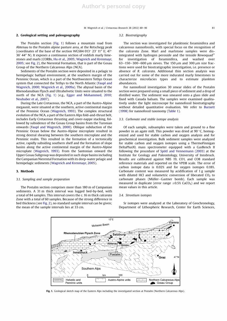
The Postalm section (Fig. 1) follows a mountain road fromAbtenau to the Postalm alpine pasture area, at the Retschegg peak(coordinates of the base of the section WGS84 013� 230 1100 E; 47�

360 4400 N). It exposes a continuous section of reddish marly lime-stones and marls (CORBs, Hu et al., 2005; Wagreich and Krenmayr,2005; see Fig. 2), the Nierental Formation, that is part of the GosauGroup of the Northern Calcareous Alps (NCA).

Sediments of the Postalm section were deposited in a pelagic tohemipelagic bathyal environment, at the southern margin of thePenninic Ocean, which is a part of the Northwestern Tethys Oceansystem that connected the Tethys to the North Atlantic (Faupl andWagreich, 2000; Wagreich et al., 2009a). The abyssal basin of theRhenodanubian Flysch and Ultrahelvetic Units were situated to thenorth of the NCA (Fig. 1) (e.g., Egger and Mohammed, 2010;Neuhuber et al., 2007).

During the Late Cretaceous, the NCA, a part of the Austro-Alpinemegaunit, were situated at the southern, active continental marginof the Penninic Ocean (Wagreich, 1993). The complex structuralevolution of the NCA, a part of the Eastern Alps fold-and-thrust belt,includes Early Cretaceous thrusting and cover-nappe stacking, fol-lowed by subsidence of the Gosau Group basins from the Turonianonwards (Faupl and Wagreich, 2000). Oblique subduction of thePenninic Ocean below the Austro-Alpine microplate resulted instrong dextral shearing between the southern microplate and thePenninic realm. This resulted in the formation of a tectonicallyactive, rapidly subsiding southern shelf and the formation of slopebasins along the active continental margin of the Austro-Alpinemicroplate (Wagreich, 1993). From the Santonian onward theUpperGosau Subgroupwas deposited in such slope basins includingthe CampanianNierental Formationwith its deep-water pelagic andhemipelagic sediments (Wagreich and Krenmayr, 2005).

3. Methods

3.1. Sampling and sample preparation

The Postalm section comprises more than 180 m of Campaniansediments. A 31 m thick interval was logged bed-by-bed, witha total of 84 samples. This interval covers the c. 16 m thick calcarataZone with a total of 60 samples. Because of the strong difference inbed thickness (see Fig. 2), no standard sample interval can be given;the mean of the sample intervals lies at 33 cm.

3.2. Biostratigraphy

The section was investigated for planktonic foraminifera andcalcareous nannofossils, with special focus on the recognition ofthe calcarata Zone. Marl and marlstone samples were dis-integrated with hydrogen peroxide and the tenside Rewoquad�

for investigation of foraminifera, and washed over63e150e300e600 mm sieves. The 150 mm and 300 mm size frac-tions were used for biostratigraphic investigation, i.e. presence orabsence of R. calcarata. Additional thin section analysis wascarried out for some of the more indurated marly limestones tocharacterize microfacies types and to estimate planktonabundances.

For nannofossil investigation 30 smear slides of the Postalmsectionwere prepared using a small piece of sediment and a drop ofdistilled water. The sediment was smeared onto a glass slide andfixed with Canada balsam. The samples were examined qualita-tively under the light microscope for nannofossil biostratigraphywithout detailed quantitative evaluation. We refer to Burnett(1998) for nannofossil taxonomy (Table 1).

3.3. Carbonate and stable isotope analysis

Of each sample, subsamples were taken and ground to a finepowder in an agate mill. This powder was dried at 90 �C, homog-enized and used for stable carbon and oxygen analysis and forgeochemical investigation. Bulk sediment samples were analyzedfor stable carbon and oxygen isotopes using a ThermoFinniganDeltaPlusXL mass spectrometer equipped with a GasBench IIfollowing the procedure of Spötl and Vennemann (2003) at theInstitute for Geology and Paleontology, University of Innsbruck.Results are calibrated against NBS 19, CO1, and CO8 standardreference materials and reported on the VPDB scale. The error ofcarbon isotope data is 0.02% and for oxygen isotopes 0.18%.Carbonate content was measured by acidification of 1 g samplewith diluted HCl and volumetric conversion of liberated CO2 tocarbonate phases (MüllereGastner bomb). Each sample wasmeasured in duplicate (error range �0.5% CaCO3) and we reportmean values in this article.

3.4. Strontium isotopes

Sr isotopes were analyzed at the Laboratory of Geochronology,Department of Lithospheric Research, Center for Earth Sciences,

Fig. 1. Geological sketch map of the Eastern Alps including the investigated section at Postalm (Northern Calcareous Alps).

M. Wagreich et al. / Cretaceous Research 38 (2012) 80e96 81


University of Vienna. Samples were leached in different concentra-tions of CH3COOH and HCl, and element separation followedconventional procedures, using an AG� 50 W-X8 (200e400 mesh,Bio-Rad) resin and HCl as elution medium. Total procedural blanksfor Sr were <1 ng. Sr fractions were loaded as chlorides and vapor-ized from a Re double filament, using a ThermoFinnigan� Triton TITIMS. A 87Sr/86Sr ratio of 0.710252� 0.000005 (n¼ 4) and0.710245� 0.000003 (n¼ 12) was determined for the NBS987 (Sr)international standard during different runs, and the ratios wererecalculated accordingly to a NIST 987 value of 0.710248 as recom-mended by McArthur et al. (2001). Within-run mass fractionationwas corrected for 86Sr/88Sr¼ 0.1194. Analytical errors of Sr isotoperatios are reported as 2s standard deviation.

To minimize the effects of diagenesis and contamination byclay particles, the strontium isotope measurements have beenperformed preferably on planktonic foraminifer tests, mainly ofthe genus Globotruncana. Planktonic foraminifera are moder-ately preserved. Tests are filled with diagenetic calcite cementand some calcite overgrowths have been recognized. Planktonicforaminiferal tests were handpicked from washed residues,cleaned in an ultrasonic bath and leached with 1N CH3COOHfor 3 h.

3.5. Orbital cyclicity and astronomical calibration

Cyclicity was investigated using variation in thickness of lime-stone and marl sequences (Fig. 2). Further we related stable carbonisotope excursions to section meters. Periodicity was obtainedusing power spectral analysis, sinusoidal regression and Morletwavelets (Hammer and Harper, 2006). Cross correlation based onsinusoidal regressions were introduced for the first time and crosscorrelations with equal and unequal intervals were calculated usingprograms developed by J.H. (see also Hohenegger and Wagreich,2012). The program packages SPSS, PAST and Excel were used forcommon statistics.

4. Results

4.1. Foraminiferal biostratigraphy

Radotruncana (Globtruncanita) calcarata (Cushman, 1927) isa species of the globotruncanid planktonic foraminifera group. Thespecies is regarded to belong to the genus Radotruncana El-Naggar,1971 (e.g., Huber et al., 2008; Petrizzo et al., 2011), or Globo-truncanita Reiss, 1957 (emended by Robaszynski et al., 1984) or tothe genera Globotruncana (e.g., Robaszynski and Caron, 1995).Radotruncana calcarata is easily recognized by its spines (peripheralextensions of chambers along sutures by tapering tubolospines,e.g., Longoria and VonFeldt, 1991). The first description of thespecies was given by Cushman (1927), the last detailed taxonomicinvestigation of the group stems from Longoria and VonFeldt(1991).

The Radotruncana calcarata Zone (e.g., Globotruncanita calcarataZone of Robaszynski et al., 1984; Caron, 1985; Robaszynski andCaron, 1995; Puckett and Mancini, 1998; Globotruncana calcarataZone of other authors, e.g., Sigal, 1977; R. calcarata Zone (KS27) ofODP/IODP zonations, e.g., Premoli Silva et al., 1998, Huber et al.,2008; zone CF10 of Li et al., 1999) is a well defined, and globallyused Late Cretaceous zone based on the total range of its nominatespecies. The calcarata Total Range Zone is widespread in low- tomid-latitude successions and recognized as a rather short timeinterval within the Late Campanian (e.g., Caron, 1985; Robaszynskiand Caron, 1995; Puckett and Mancini, 1998). The relatively shorttaxon range of the nominate taxon led to the definition of a totalrange zone (e.g., Robaszynski and Caron, 1995; Puckett andMancini, 1998).

For a long time the last occurrence (LO) of R. calcarata, and thusthe top of the calcarata Total Range Zone, was interpreted torepresent the base of the Maastrichtian, especially in Tethyansections (e.g., Caron, 1985). This was corrected by Schönfeld andBurnett (1991), who recognized that the zone is well within the

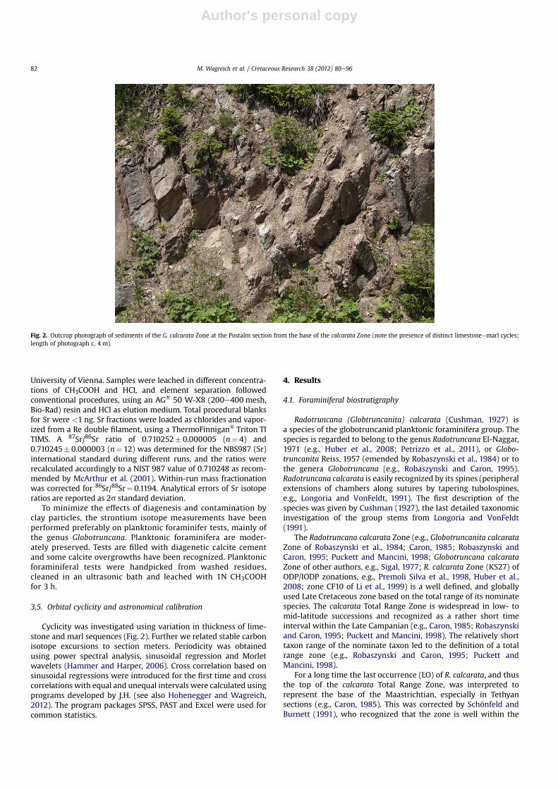
Fig. 2. Outcrop photograph of sediments of the G. calcarata Zone at the Postalm section from the base of the calcarata Zone (note the presence of distinct limestoneemarl cycles;length of photograph c. 4 m).

M. Wagreich et al. / Cretaceous Research 38 (2012) 80e9682


Table

1Calcareou

snan

nofossild

istribution

inthePo

stalm

section.



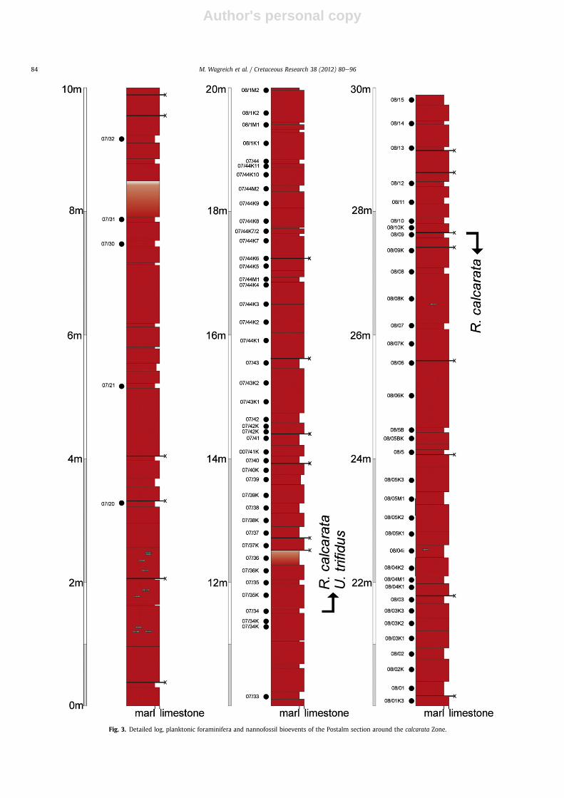
Fig. 3. Detailed log, planktonic foraminifera and nannofossil bioevents of the Postalm section around the calcarata Zone.



Late Campanian and far below the base of the Maastrichtian asdefined by belemnites in the boreal-temperate realm. Our workidentifies the calcarata Zone as a short time interval of less than1 Ma within the Late Campanian (or even within the middleCampanian). However, the exact position of the calcarata Zone inrespect to macrofossil biostratigraphic scales, the GSSP section ofthe CampanianeMaastrichtian boundary at Tercis, France (Odinand Lamaurelle, 2001) and the chalk sections of England andNorthern Germany remains unclear or only loosely constrained bystepwise correlation with different fossil groups or chemo-stratigraphy. The stratigraphic position of the calcarata Zone withinthe Late Campanian ammonite zonation and its relation to the FO ofthe ammonite Pachydiscus neubergicus as a primary marker for thebase of the Maastrichtian was confirmed by Ion and Odin (2001) inthe Maastrichtian GSSP at Tercis (France) and correlated Spanishsections (Küchler et al., 2001). Although the presence and actualrange of R. calcarata remains somehow dubious at Tercis, based onseveral differing parallel studies and the problem of thin section vs.washed sample data (compare Ion and Odin, 2001), the range in theGSSP section lateron was more secured (Odin et al., 2004; Odin,2010).

Within the investigated part of the Postalm section R. calcaratastarts at 11.53 m and ranges up to 27.61 m, resulting in a zonal

thickness of 16.08 m (Fig. 3). Samples below that interval can beattributed to the Globotruncana ventricosa Zone (or Con-tusotruncana plummerae Zone of Petrizzo et al., 2011), samplesabove to the Globotruncanella havanensis Zone. The focus of thisresearch was to identify the calcarata Zone and did not includea detailed survey of planktonic foraminifera.

4.2. Calcareous nannofossil biostratigraphy

Based on nannofossil marker species, the investigated sectioncan be divided into two nannofossil standard zones (Table 1): (1)CC21 of Perch-Nielsen (1985) e UC15cTP of Burnett (1998), at thePostalm section from 0 m to 11.50 m, defined by the presence ofQuadrum (Uniplanarius) sissinghii and additional markers likeBroinsonia parca parca, Broinsonia parca constricta, Reinhardtitesanthophorus, Reinhardtites cf. levis and Ceratolithoides aculeus; and(2) CC22abeUC15deTP, from11.53 muntil the top of the investigatedsection, defined by the FO of Uniplanarius(Quadrum) trifidus and thecontinuous presence of Reinhardtites anthophorus. Eiffellithus exi-mius, which normally is still present in these zones (e.g., Burnett,1998), was not found in the calcarata Zone of the Postalm section.

Direct correlations of nannofossils and planktic foraminiferzonations (e.g., Wagreich and Krenmayr, 1993; Gardin et al., 2001;

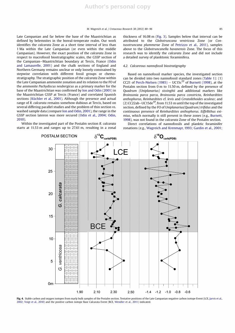
Fig. 4. Stable carbon and oxygen isotopes frommarly bulk samples of the Postalm section. Tentative positions of the Late Campanian negative carbon isotope Event (LCE, Jarvis et al.,2002; Voigt et al., 2010) and the positive carbon isotope Base Calcarata Event (BCE, Wendler et al., 2011) indicated.



Küchler et al., 2001; see also Ogg et al., 2004) indicate that the FO ofR. calcarata is roughly equivalent to or slightly above the FO ofU. trifidus. In the investigated section the FO of R. calcarata and theFO of Uniplanarius (Quadrum) trifidus co-occur in the same sample(Fig. 3). The LO of R. calcarata still falls into CC22abeUC15deTP,below the LO of Reinhardtites anthophorus and Eiffellithus eximius.The data compiled by Odin and Lamaurelle (2001) on the GlobalBoundary Section and Stratotype (GSSP) at Tercis, southern Franceof the lower boundary of the Maastrichtian, indicate a fairly similarpicture, although nannofossil data by several involved specialistsare controversial as first and last occurrences of some nannofossilmarkers were placed differently in the GSSP section (see Gardinet al., 2001).

Despite a moderate to poor preservation, nannofossil assem-blages are diverse with 50 taxa. Assemblages are dominated bycommon Watznaueria barnesae. Other common taxa (more than 1specimen per field of view) include Micula staurophora, Cri-brosphaerella ehrenbergii, Lucianorhabdus cayeuxii, Prediscosphaeracretacea, and Retecapsa crenulata. Typical low- to mid-latitude“Tethyan” nannofossils such as Ceratolithoides aculeus, Uni-planarius (Quadrum) trifidus and Uniplanarius(Quadrum) sissinghibesides relatively high amounts of Watznaueria ssp. support theTethyan character of the nannofossil assemblage. Cooler water“boreal” species like Kamptnerius magnificus are rare.

4.3. Stable carbon and oxygen isotopes

Although diagenesis plays some role, largely primary values andtrends are recorded in the carbon isotope values. Stable carbonisotope concentration of bulk sediments ranges in general between2 and 2.5& VPDB (Fig. 4). Marly intervals are less prone to

diagenetic alteration (e.g., Westphal and Munnecke, 2003) there-fore we concentrate on analyses of marly lithologies. A negativeexcursion (minimum at 2.04& VPDB) below the calcarata Zone isfollowed by a first positive excursion (double peak at 2.36& VPDB)within the zone at 12.00e12.45 m. A negative excursion witha peak of 2.20& VPDB at 15.55 m and a positive excursion at18.81 m (2.35& VPDB) are followed by a gradual decrease withminor wiggles and a final positive peak at the top of the calcarataZone at 27.61 m (again at 2.35& VPDB). Above the zone a negativeexcursion is present at 29.02 m (2.04& VPDB).

Stable oxygen isotopes are e compared to carbon isotopes e

more readilyaffected bydiagenetic alteration (Anderson andArthur,1983) and regarded as less reliable in Alpine sections (e.g., Neuhuberet al., 2007). Bulkoxygen isotopesofmarl bedsof thePostalmsectionshow a decreasing trend from values around �0.80& at the base ofthe zone to values around �1.20& at the top.

4.4. Strontium isotope stratigraphy

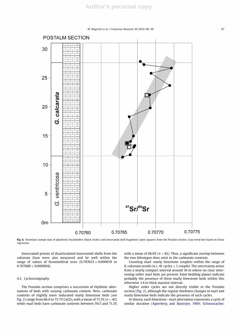
Corrected values adjusted to the NBS987 (Sr) internationalstandard give a range of strontium isotope ratios for the calcarataZone of 0.707655� 0.000018e0.707722� 0.000004 in the Postalmsection (mean of 15 samples 0.707679). Slightly higher values arerecorded up-section (Fig. 6), that is in accordance with the generalincreasing trend of strontium isotope values during theCampanianeMaastrichtian (McArthur et al., 2001; McArthur andHowarth, 2004). Some scatter in the data is present due todiagenesis. Largely similar values of 0.707667� 0.000009 (GosauValley area) and 0.707673� 0.000009e0.707671�0.000012(Gams basin) have also been obtained from the calcarata Zone inother Austrian sections (Wagreich, unpublished data).

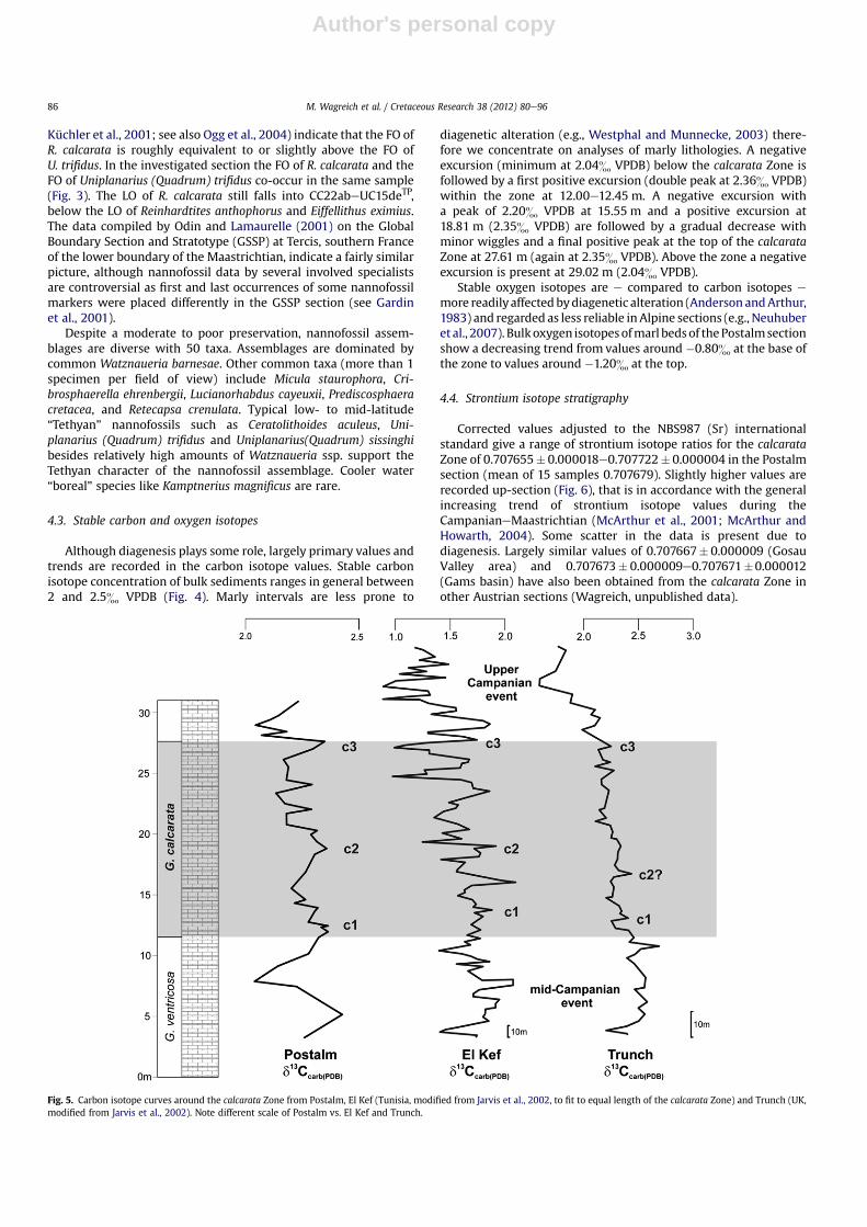
Fig. 5. Carbon isotope curves around the calcarata Zone from Postalm, El Kef (Tunisia, modified from Jarvis et al., 2002, to fit to equal length of the calcarata Zone) and Trunch (UK,modified from Jarvis et al., 2002). Note different scale of Postalm vs. El Kef and Trunch.



Inoceramid prisms of disarticulated inoceramid shells from thecalcarata Zone were also measured and lie well within therange of values of foraminiferal tests (0.707653� 0.000019 to0.707680� 0.000004).

4.5. Cyclostratigraphy

The Postalm section comprises a succession of rhythmic alter-nations of beds with varying carbonate content. Here, carbonatecontents of slightly more indurated marly limestone beds (seeFig. 2) range from 66.4 to 75.7% CaCO3with amean of 71.3% (n¼ 42)while marl beds have carbonate contents between 59.5 and 71.3%

with a mean of 66.0% (n¼ 42). Thus, a significant overlap betweenthe two lithotypes does exist in the carbonate contents.

Counting marlemarly limestone couplets within the range ofR. calcarata results in c. 41 cycles� 1 couplet. The uncertainty arisesfrom a nearly compact interval around 16 m where no clear inter-vening softer marl beds are present. Faint bedding planes indicateprobably the presence of three marly limestone beds within thisotherwise 1.4 m thick massive interval.

Higher order cycles are not directly visible in the Postalmsection (Fig. 2), although the regular thickness changes in marl andmarly limestone beds indicate the presence of such cycles.

In theory, each limestoneemarl alternation represents a cycle ofsimilar duration (Agterberg and Banerjee, 1969; Schwarzacher,

Fig. 6. Strontium isotope data of planktonic foraminifers (black circles) and inoceramid shell fragments (open squares) from the Postalm section. Gray trend line based on linearregression.



1975). Accordingly, varying thickness changes of limestone andmarls may represent a set of superior cycles. Although differentialcompaction and diagenesis may have altered the primary thicknesssignal to some extent, the presence of a primary signal recorded inlimestoneemarl couplets in the sense of Westphal et al. (2010) isevident from heterolithic fillings of burrows (Zoophycos andChondrites-type) and from the fact that strontium isotope andcarbon isotope values of bulk carbonate arewell within the range ofCampanian marine values.

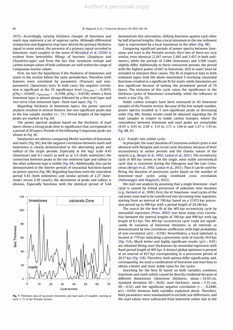
First, we test the hypothesis if the thickness of limestones andmarls in the section follow the same periodicities. Therefore bothfeatures were correlated by parametric (Pearson) and non-parametric (Spearman) tests. In both cases, the negative correla-tion is significant at the 5% significance level (rPearson¼�0.2033,p(H0)¼ 0.0445; rSpearman¼�0.2198, p(H0)¼ 0.0328) where a thicklimestone layer is almost always followed by a thin marl layer andvice versa (thin limestone layerethick marl layer; Fig. 7).

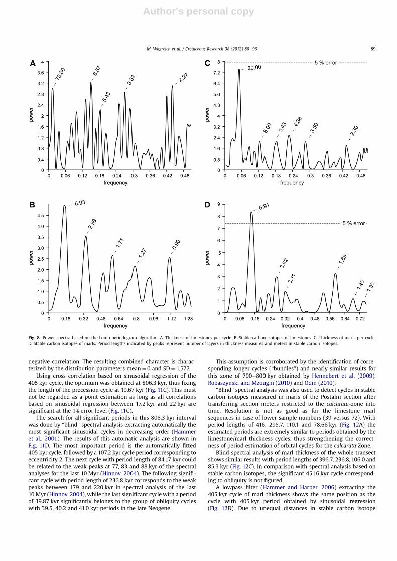
Regarding thickness in limestone layers, the power spectralanalysis resulted in several distinct, but non-significant peaks dueto the low sample number (n¼ 71). Period lengths of the highestpeaks are marked in Fig. 8A.

The power spectral analysis based on the thickness of marllayers shows a strong peak close to significance that corresponds toa period of 20 layers. Periods of the following 5 important peaks areshown in Fig. 8C.

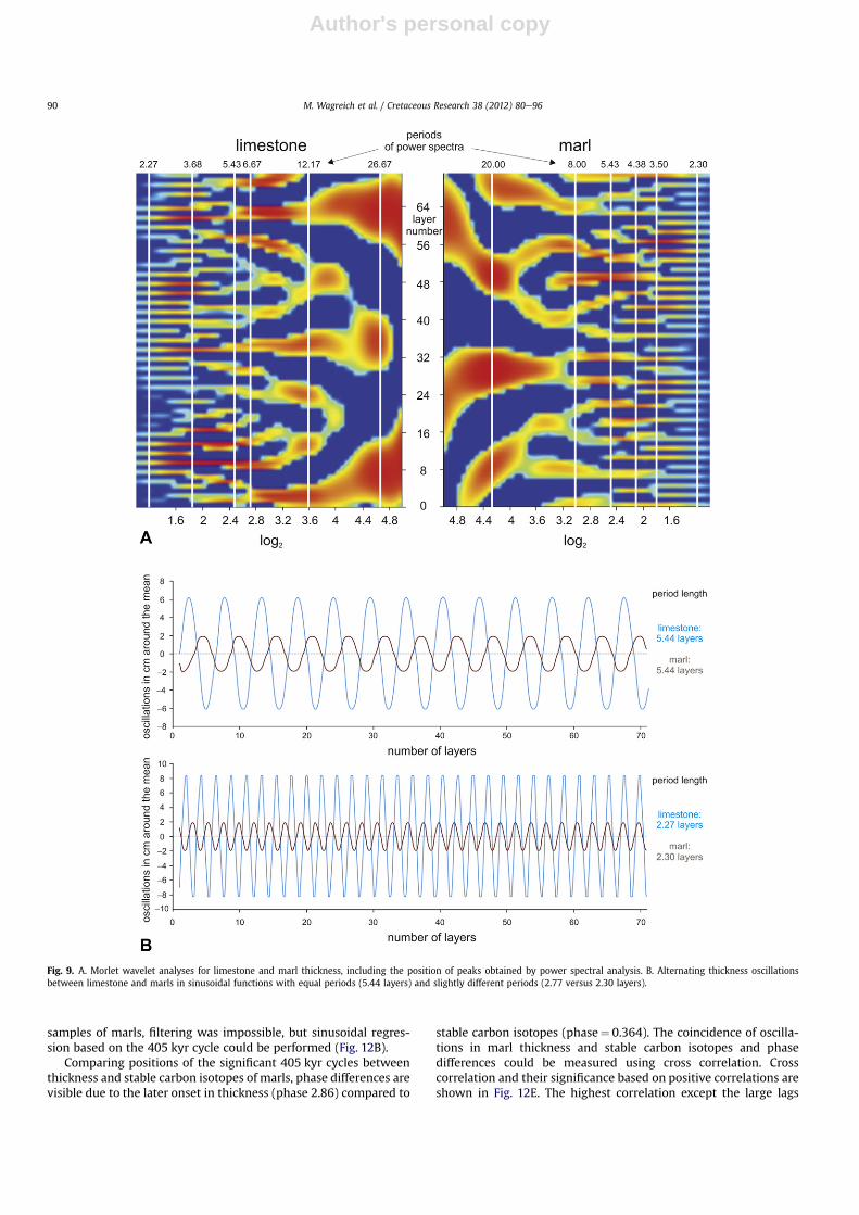
Similarities are obvious comparingMorlet wavelets of limestoneandmarls (Fig. 9A), but the negative correlation betweenmarls andlimestones is clearly demonstrated in the alternating peaks andvalleys of the larger periods. Especially at the log2 scale 4.45(limestone) and 4.3 (marl) as well as at 3.5 (both sediments) theconnection between peaks in the one sediment type and valleys inthe other sediment type is visible (Fig. 9A). Additionally, this can bedemonstrated in the shorter periods of sinusoidal functions basedon power spectra (Fig. 9B). Regarding functions with the coincidentperiod 5.43 (both sediments) and similar periods of 2.27 (lime-stone) versus 2.30 (marls), the alternation of peaks and valleys isobvious. Especially functions with the identical period of 5.44

demonstrate this alternation, shifting functions against each otherby half of period lengths; thus a local minimum in the one sedimenttype is represented by a local maximum in the other (Fig. 9B).

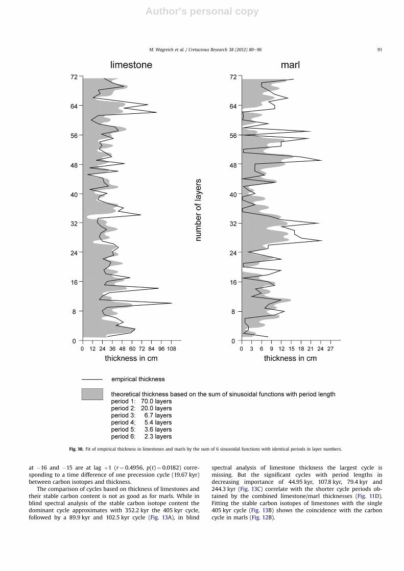
Comparing significant periods of power spectra between lime-stone and marl in the Postalm section, then two of them are verysimilar, even identical (2.267 versus 2.305 and 5.437 in both sedi-ments), while the periods of 3.684 (limestone) and 3.500 (marl)slightly differ. Additionally to these concurrent periods, the periodwith the highest power (6.667 in limestone, 20.0 in marl) must beincluded to interpret their causes. The fit of empirical data in bothsediment types with the above mentioned 5 overlying sinusoidalfunctions resulted in a significant fit for marls, while limestones areless significant because of lacking the prominent period of 70layers. The inclusion of this cycle raises the significance in thethickness cycles of limestones remarkably, while the influence inmarls is low (Fig. 10).

Stable carbon isotopes have been measured in 43 limestonesamples of the Postalm section. Because of the low sample number,power spectra resulted in 5 non-significant peaks in decreasingorder (Fig. 8B). Similar results could be obtained regarding the 39marl samples in respect to stable carbon isotopes, where thecoincidence between limestone and marl peaks are remarkable(6.93 v. 6.91 m, 2.99 v. 3.11 m, 1.71 v. 1.69 m and 1.27 v. 1.35 m;Fig. 8B, D).

4.5.1. Transfer into orbital cyclesIn principle, the exact duration of Cretaceous orbital cycles is not

identical with Neogene and recent cycle durations, because of theirinconsistency in earlier periods and the chaotic nature of thesystem (e.g., Berger et al., 1992; Laskar et al., 2011). The eccentricitycycle of 405 kyr seems to be the single, most stable astronomicalcycle that is consistent during the Paleogene and the Late Creta-ceous (Berger et al., 1992; Laskar et al., 2011). Thus it can be used forfitting the duration of precession cycles based on the number oflimestoneemarl cycles using combined cross correlation(Hohenegger and Wagreich, 2012).

We start our analysis by assuming that a single limestoneemarlcycle is caused by orbital precession of unknown time duration(e.g., Herbert et al., 1999). First, the 41 limestoneemarl cycles of thecalcarata-zone had to be transferred into increasing time segments,starting from an interval of 700 kyr based on a 17.073 kyr preces-sion period up to 990 kyr with a period length of 24.146 kyr.

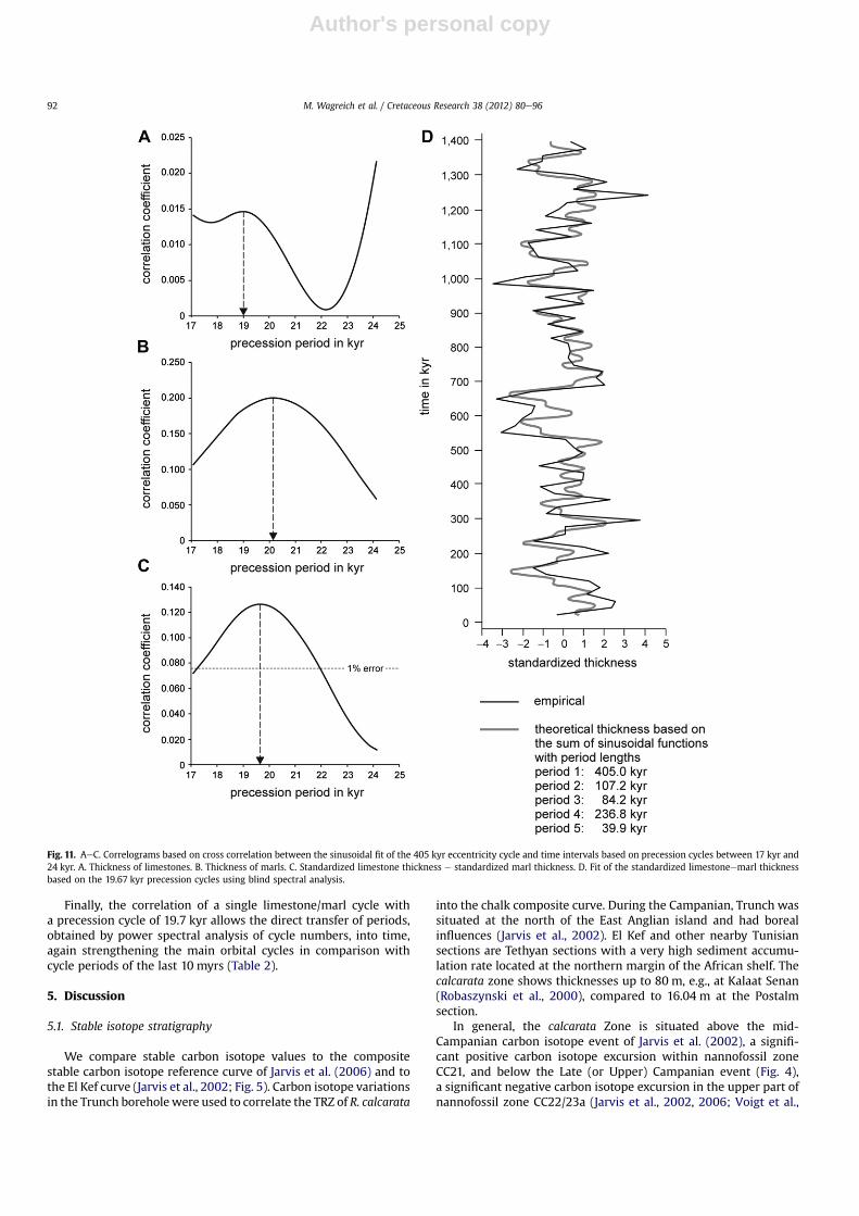
The search for the best fit of the 405 kyr eccentricity cycle bysinusoidal regression (Press, 2002) was done using cross correla-tion between the interval lengths of 700 kyr and 990 kyr with laglength of 0.1 kyr. The 405 kyr eccentricity cycle could not signifi-cantly fit variation of limestone thickness in all intervals asdemonstrated by low correlation coefficients with high probabilityof non-correlation (p(t)> 0.156). Nevertheless, a local optimum islocated at 779 kyr indicating a precession cycle of exactly 19.0 kyr(Fig. 11A). Much better and highly significant results (p(t)< 0.01)are obtained fitting marl thicknesses by sinusoidal regression withfixed period length of 405 kyr. A distinct global optimum is presentat an interval of 827 kyr corresponding to a precession period of20.17 kyr (Fig. 11B). Therefore, both optima differ significantly, and,consequently, we used a combination of limestone andmarl data toobtain a better and more stable value for the cycles.

Searching for the best fit based on both variables combineslimestone and marls which cannot be directly combined because ofdifferent dimensions (limestone thickness: mean¼ 33.93 cm,standard deviation SD¼ 18.02; marl thickness: mean¼ 7.33 cm,SD¼ 6.52) and the significant negative correlation (r¼�0.2440,p(t)¼ 0.019) between both variables explained above. Therefore,both parameters were standardized to exclude size differences, andthe marl values were subtracted from limestone values due to the

Fig. 7. Thickness data of successive limestone and marl parts of couplets, starting atcycle 1e71 of the Postalm section.



negative correlation. The resulting combined character is charac-terized by the distribution parameters mean¼ 0 and SD¼ 1.577.

Using cross correlation based on sinusoidal regression of the405 kyr cycle, the optimum was obtained at 806.3 kyr, thus fixingthe length of the precession cycle at 19.67 kyr (Fig. 11C). This mustnot be regarded as a point estimation as long as all correlationsbased on sinusoidal regression between 17.2 kyr and 22 kyr aresignificant at the 1% error level (Fig. 11C).

The search for all significant periods in this 806.3 kyr intervalwas done by “blind” spectral analysis extracting automatically themost significant sinusoidal cycles in decreasing order (Hammeret al., 2001). The results of this automatic analysis are shown inFig. 11D. The most important period is the automatically fitted405 kyr cycle, followed by a 107.2 kyr cycle period corresponding toeccentricity 2. The next cycle with period length of 84.17 kyr couldbe related to the weak peaks at 77, 83 and 88 kyr of the spectralanalyses for the last 10 Myr (Hinnov, 2004). The following signifi-cant cycle with period length of 236.8 kyr corresponds to the weakpeaks between 179 and 220 kyr in spectral analysis of the last10 Myr (Hinnov, 2004), while the last significant cycle with a periodof 39.87 kyr significantly belongs to the group of obliquity cycleswith 39.5, 40.2 and 41.0 kyr periods in the late Neogene.

This assumption is corroborated by the identification of corre-sponding longer cycles (“bundles”) and nearly similar results forthis zone of 790e800 kyr obtained by Hennebert et al. (2009),Robaszynski and Mzoughi (2010) and Odin (2010).

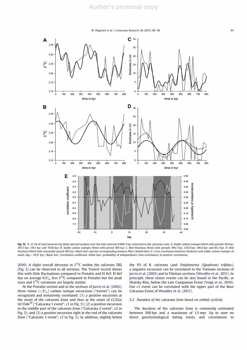
“Blind” spectral analysis was also used to detect cycles in stablecarbon isotopes measured in marls of the Postalm section aftertransferring section meters restricted to the calcarata-zone intotime. Resolution is not as good as for the limestoneemarlsequences in case of lower sample numbers (39 versus 72). Withperiod lengths of 416, 295.7, 110.1 and 78.66 kyr (Fig. 12A) theestimated periods are extremely similar to periods obtained by thelimestone/marl thickness cycles, thus strengthening the correct-ness of period estimation of orbital cycles for the calcarata Zone.

Blind spectral analysis of marl thickness of the whole transectshows similar results with period lengths of 396.7, 236.8, 106.0 and85.3 kyr (Fig. 12C). In comparison with spectral analysis based onstable carbon isotopes, the significant 45.16 kyr cycle correspond-ing to obliquity is not figured.

A lowpass filter (Hammer and Harper, 2006) extracting the405 kyr cycle of marl thickness shows the same position as thecycle with 405 kyr period obtained by sinusoidal regression(Fig. 12D). Due to unequal distances in stable carbon isotope

Fig. 8. Power spectra based on the Lomb periodogram algorithm. A. Thickness of limestones per cycle. B. Stable carbon isotopes of limestones. C. Thickness of marls per cycle.D. Stable carbon isotopes of marls. Period lengths indicated by peaks represent number of layers in thickness measures and meters in stable carbon isotopes.



samples of marls, filtering was impossible, but sinusoidal regres-sion based on the 405 kyr cycle could be performed (Fig. 12B).

Comparing positions of the significant 405 kyr cycles betweenthickness and stable carbon isotopes of marls, phase differences arevisible due to the later onset in thickness (phase 2.86) compared to

stable carbon isotopes (phase¼ 0.364). The coincidence of oscilla-tions in marl thickness and stable carbon isotopes and phasedifferences could be measured using cross correlation. Crosscorrelation and their significance based on positive correlations areshown in Fig. 12E. The highest correlation except the large lags

Fig. 9. A. Morlet wavelet analyses for limestone and marl thickness, including the position of peaks obtained by power spectral analysis. B. Alternating thickness oscillationsbetween limestone and marls in sinusoidal functions with equal periods (5.44 layers) and slightly different periods (2.77 versus 2.30 layers).



at �16 and �15 are at lag þ1 (r¼ 0.4956, p(t)¼ 0.0182) corre-sponding to a time difference of one precession cycle (19.67 kyr)between carbon isotopes and thickness.

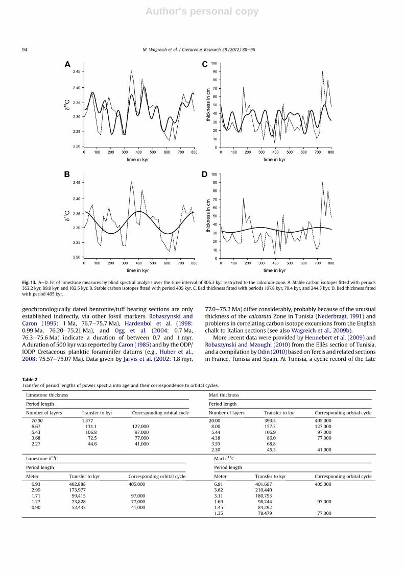
The comparison of cycles based on thickness of limestones andtheir stable carbon content is not as good as for marls. While inblind spectral analysis of the stable carbon isotope content thedominant cycle approximates with 352.2 kyr the 405 kyr cycle,followed by a 89.9 kyr and 102.5 kyr cycle (Fig. 13A), in blind

spectral analysis of limestone thickness the largest cycle ismissing. But the significant cycles with period lengths indecreasing importance of 44.95 kyr, 107.8 kyr, 79.4 kyr and244.3 kyr (Fig. 13C) correlate with the shorter cycle periods ob-tained by the combined limestone/marl thicknesses (Fig. 11D).Fitting the stable carbon isotopes of limestones with the single405 kyr cycle (Fig. 13B) shows the coincidence with the carboncycle in marls (Fig. 12B).

Fig. 10. Fit of empirical thickness in limestones and marls by the sum of 6 sinusoidal functions with identical periods in layer numbers.



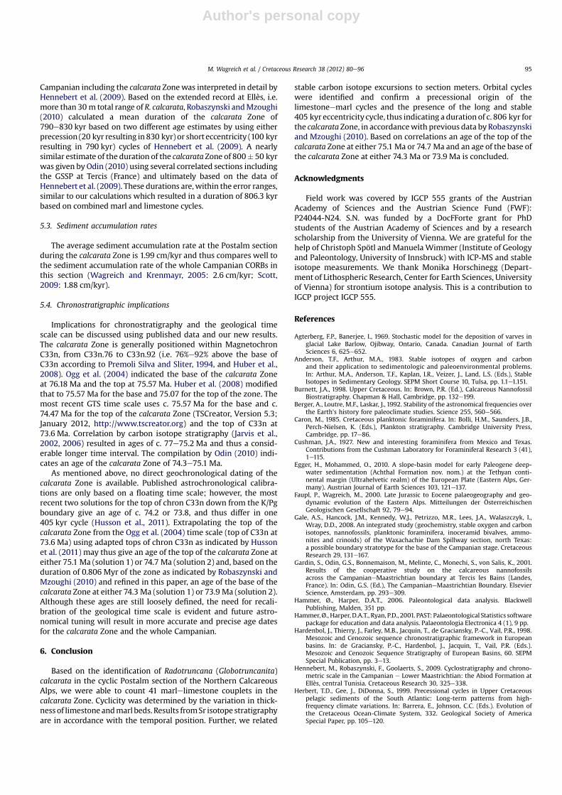
Finally, the correlation of a single limestone/marl cycle witha precession cycle of 19.7 kyr allows the direct transfer of periods,obtained by power spectral analysis of cycle numbers, into time,again strengthening the main orbital cycles in comparison withcycle periods of the last 10 myrs (Table 2).

5. Discussion

5.1. Stable isotope stratigraphy

We compare stable carbon isotope values to the compositestable carbon isotope reference curve of Jarvis et al. (2006) and tothe El Kef curve (Jarvis et al., 2002; Fig. 5). Carbon isotope variationsin the Trunch boreholewere used to correlate the TRZ of R. calcarata

into the chalk composite curve. During the Campanian, Trunch wassituated at the north of the East Anglian island and had borealinfluences (Jarvis et al., 2002). El Kef and other nearby Tunisiansections are Tethyan sections with a very high sediment accumu-lation rate located at the northern margin of the African shelf. Thecalcarata zone shows thicknesses up to 80 m, e.g., at Kalaat Senan(Robaszynski et al., 2000), compared to 16.04 m at the Postalmsection.

In general, the calcarata Zone is situated above the mid-Campanian carbon isotope event of Jarvis et al. (2002), a signifi-cant positive carbon isotope excursion within nannofossil zoneCC21, and below the Late (or Upper) Campanian event (Fig. 4),a significant negative carbon isotope excursion in the upper part ofnannofossil zone CC22/23a (Jarvis et al., 2002, 2006; Voigt et al.,

Fig. 11. AeC. Correlograms based on cross correlation between the sinusoidal fit of the 405 kyr eccentricity cycle and time intervals based on precession cycles between 17 kyr and24 kyr. A. Thickness of limestones. B. Thickness of marls. C. Standardized limestone thickness e standardized marl thickness. D. Fit of the standardized limestoneemarl thicknessbased on the 19.67 kyr precession cycles using blind spectral analysis.



2010). A slight overall decrease in d13C within the calcarata TRZ(Fig. 5) can be observed in all sections. The Trunch record showsthis with little fluctuations compared to Postalm and El Kef. El Kefhas on average 0.5& less d13C compared to Postalm but the peaksizes and d13C variations are largely similar.

At the Postalm section and in the sections of Jarvis et al. (2002),three minor (<5&) carbon isotope excursions (“events”) can berecognized and tentatively correlated: (1) a positive excursion atthe onset of the calcarata Zone and thus at the onset of CC22a/UC15deTP (“Calcarata 1 event”, c1 in Fig. 5); (2) a positive excursionin the middle part of the calcarata Zone (“Calcarata 2 event”, c2 inFig. 5); and (3) a positive excursion right at the end of the calcarataZone (“Calcarata 3 event”, c3 in Fig. 5). In addition, slightly below

the FO of R. calcarata (and Uniplanarius (Quadrum) trifidus),a negative excursion can be correlated to the Tunisian sections ofJarvis et al. (2002) and to Tibetian sections (Wendler et al., 2011). Inprinciple, these minor events can be also found in the Pacific, atShatsky Rise, below the Late Campanian Event (Voigt et al., 2010).Our c1 event can be correlated with the upper part of the BaseCalcarata Event of Wendler et al. (2011).

5.2. Duration of the calcarata Zone based on orbital cyclicity

The duration of the calcarata Zone is commonly estimatedbetween 500 kyr and a maximum of 1.5 myr. Up to now nodirect geochronological dating exists, and correlations to

Fig. 12. AeD. Fit of marl measures by blind spectral analysis over the time interval of 806.3 kyr restricted to the calcarata-zone. A. Stable carbon isotopes fitted with periods 416 kyr,295.7 kyr, 110.1 kyr and 78.66 kyr. B. Stable carbon isotopes fitted with period 405 kyr. C. Bed thickness fitted with periods 396.7 kyr, 236.8 kyr, 106.0 kyr and 85.3 kyr. D. Bedthickness fitted with sinusoidal period 405 kyr (black line) and the corresponding lowpass filter (dotted line). E. Cross correlation between thickness and stable carbon isotopes ofmarls (lag¼ 19.67 kyr). Black line: Correlation coefficient, white line: probability of independence (non-correlation) in positive correlations.



geochronologically dated bentonite/tuff bearing sections are onlyestablished indirectly, via other fossil markers. Robaszynski andCaron (1995: 1 Ma, 76.7e75.7 Ma), Hardenbol et al. (1998:0.99 Ma, 76.20e75.21 Ma), and Ogg et al. (2004: 0.7 Ma,76.3e75.6 Ma) indicate a duration of between 0.7 and 1 myr.A duration of 500 kyr was reported by Caron (1985) and by the ODP/IODP Cretaceous planktic foraminifer datums (e.g., Huber et al.,2008: 75.57e75.07 Ma). Data given by Jarvis et al. (2002: 1.8 myr,

77.0e75.2 Ma) differ considerably, probably because of the unusualthickness of the calcarata Zone in Tunisia (Nederbragt, 1991) andproblems in correlating carbon isotope excursions from the Englishchalk to Italian sections (see also Wagreich et al., 2009b).

More recent data were provided by Hennebert et al. (2009) andRobaszynski and Mzoughi (2010) from the Ellès section of Tunisia,anda compilationbyOdin (2010)basedonTercis and related sectionsin France, Tunisia and Spain. At Tunisia, a cyclic record of the Late

Fig. 13. AeD. Fit of limestone measures by blind spectral analysis over the time interval of 806.3 kyr restricted to the calcarata-zone. A. Stable carbon isotopes fitted with periods352.2 kyr, 89.9 kyr, and 102.5 kyr. B. Stable carbon isotopes fitted with period 405 kyr. C. Bed thickness fitted with periods 107.8 kyr, 79.4 kyr, and 244.3 kyr. D. Bed thickness fittedwith period 405 kyr.

Table 2Transfer of period lengths of power spectra into age and their correspondence to orbital cycles.

Limestone thickness Marl thickness

Period length Period length

Number of layers Transfer to kyr Corresponding orbital cycle Number of layers Transfer to kyr Corresponding orbital cycle

70.00 1,377 20.00 393.3 405,0006.67 131.1 127,000 8.00 157.3 127,0005.43 106.8 97,000 5.44 106.9 97,0003.68 72.5 77,000 4.38 86.0 77,0002.27 44.6 41,000 3.50 68.8

2.30 45.3 41,000

Limestone d13C Marl d13C

Period length Period length

Meter Transfer to kyr Corresponding orbital cycle Meter Transfer to kyr Corresponding orbital cycle

6.93 402,888 405,000 6.91 401,697 405,0002.99 173,977 3.62 210,4401.71 99,415 97,000 3.11 180,7931.27 73,828 77,000 1.69 98,244 97,0000.90 52,433 41,000 1.45 84,292

1.35 78,479 77,000



Campanian including the calcarata Zonewas interpreted in detail byHennebert et al. (2009). Based on the extended record at Ellès, i.e.more than 30 m total range of R. calcarata, Robaszynski andMzoughi(2010) calculated a mean duration of the calcarata Zone of790e830 kyr based on two different age estimates by using eitherprecession (20 kyr resulting in 830 kyr) or short eccentricity (100 kyrresulting in 790 kyr) cycles of Hennebert et al. (2009). A nearlysimilar estimate of the duration of the calcarata Zone of 800� 50 kyrwas given by Odin (2010) using several correlated sections includingthe GSSP at Tercis (France) and ultimately based on the data ofHennebert et al. (2009). These durations are,within the error ranges,similar to our calculations which resulted in a duration of 806.3 kyrbased on combined marl and limestone cycles.

5.3. Sediment accumulation rates

The average sediment accumulation rate at the Postalm sectionduring the calcarata Zone is 1.99 cm/kyr and thus compares well tothe sediment accumulation rate of the whole Campanian CORBs inthis section (Wagreich and Krenmayr, 2005: 2.6 cm/kyr; Scott,2009: 1.88 cm/kyr).

5.4. Chronostratigraphic implications

Implications for chronostratigraphy and the geological timescale can be discussed using published data and our new results.The calcarata Zone is generally positioned within MagnetochronC33n, from C33n.76 to C33n.92 (i.e. 76%e92% above the base ofC33n according to Premoli Silva and Sliter, 1994, and Huber et al.,2008). Ogg et al. (2004) indicated the base of the calcarata Zoneat 76.18 Ma and the top at 75.57 Ma. Huber et al. (2008) modifiedthat to 75.57 Ma for the base and 75.07 for the top of the zone. Themost recent GTS time scale uses c. 75.57 Ma for the base and c.74.47 Ma for the top of the calcarata Zone (TSCreator, Version 5.3;January 2012, http://www.tscreator.org) and the top of C33n at73.6 Ma. Correlation by carbon isotope stratigraphy (Jarvis et al.,2002, 2006) resulted in ages of c. 77e75.2 Ma and thus a consid-erable longer time interval. The compilation by Odin (2010) indi-cates an age of the calcarata Zone of 74.3e75.1 Ma.

As mentioned above, no direct geochronological dating of thecalcarata Zone is available. Published astrochronological calibra-tions are only based on a floating time scale; however, the mostrecent two solutions for the top of chron C33n down from the K/Pgboundary give an age of c. 74.2 or 73.8, and thus differ in one405 kyr cycle (Husson et al., 2011). Extrapolating the top of thecalcarata Zone from the Ogg et al. (2004) time scale (top of C33n at73.6 Ma) using adapted tops of chron C33n as indicated by Hussonet al. (2011) may thus give an age of the top of the calcarata Zone ateither 75.1 Ma (solution 1) or 74.7 Ma (solution 2) and, based on theduration of 0.806 Myr of the zone as indicated by Robaszynski andMzoughi (2010) and refined in this paper, an age of the base of thecalcarata Zone at either 74.3 Ma (solution 1) or 73.9 Ma (solution 2).Although these ages are still loosely defined, the need for recali-bration of the geological time scale is evident and future astro-nomical tuning will result in more accurate and precise age datesfor the calcarata Zone and the whole Campanian.

6. Conclusion

Based on the identification of Radotruncana (Globotruncanita)calcarata in the cyclic Postalm section of the Northern CalcareousAlps, we were able to count 41 marlelimestone couplets in thecalcarata Zone. Cyclicity was determined by the variation in thick-ness of limestone andmarl beds. Results fromSr isotope stratigraphyare in accordance with the temporal position. Further, we related

stable carbon isotope excursions to section meters. Orbital cycleswere identified and confirm a precessional origin of thelimestoneemarl cycles and the presence of the long and stable405 kyr eccentricity cycle, thus indicating a duration of c. 806 kyr forthe calcarata Zone, in accordancewith previous data byRobaszynskiand Mzoughi (2010). Based on correlations an age of the top of thecalcarata Zone at either 75.1 Ma or 74.7 Ma and an age of the base ofthe calcarata Zone at either 74.3 Ma or 73.9 Ma is concluded.

Acknowledgments

Field work was covered by IGCP 555 grants of the AustrianAcademy of Sciences and the Austrian Science Fund (FWF):P24044-N24. S.N. was funded by a DocFForte grant for PhDstudents of the Austrian Academy of Sciences and by a researchscholarship from the University of Vienna. We are grateful for thehelp of Christoph Spötl and Manuela Wimmer (Institute of Geologyand Paleontology, University of Innsbruck) with ICP-MS and stableisotope measurements. We thank Monika Horschinegg (Depart-ment of Lithospheric Research, Center for Earth Sciences, Universityof Vienna) for strontium isotope analysis. This is a contribution toIGCP project IGCP 555.

References

Agterberg, F.P., Banerjee, I., 1969. Stochastic model for the deposition of varves inglacial Lake Barlow, Ojibway, Ontario, Canada. Canadian Journal of EarthSciences 6, 625e652.

Anderson, T.F., Arthur, M.A., 1983. Stable isotopes of oxygen and carbonand their application to sedimentologic and paleoenvironmental problems.In: Arthur, M.A., Anderson, T.F., Kaplan, I.R., Veizer, J., Land, L.S. (Eds.), StableIsotopes in Sedimentary Geology. SEPM Short Course 10, Tulsa, pp. 1.1e1.151.

Burnett, J.A., 1998. Upper Cretaceous. In: Brown, P.R. (Ed.), Calcareous NannofossilBiostratigraphy. Chapman & Hall, Cambridge, pp. 132e199.

Berger, A., Loutre, M.F., Laskar, J., 1992. Stability of the astronomical frequencies overthe Earth’s history fore paleoclimate studies. Science 255, 560e566.

Caron, M., 1985. Cretaceous planktonic foraminifera. In: Bolli, H.M., Saunders, J.B.,Perch-Nielsen, K. (Eds.), Plankton stratigraphy. Cambridge University Press,Cambridge, pp. 17e86.

Cushman, J.A., 1927. New and interesting foraminifera from Mexico and Texas.Contributions from the Cushman Laboratory for Foraminiferal Research 3 (41),1e115.

Egger, H., Mohammed, O., 2010. A slope-basin model for early Paleogene deep-water sedimentation (Achthal Formation nov. nom.) at the Tethyan conti-nental margin (Ultrahelvetic realm) of the European Plate (Eastern Alps, Ger-many). Austrian Journal of Earth Sciences 103, 121e137.

Faupl, P., Wagreich, M., 2000. Late Jurassic to Eocene palaeogeography and geo-dynamic evolution of the Eastern Alps. Mitteilungen der ÖsterreichischenGeologischen Gesellschaft 92, 79e94.

Gale, A.S., Hancock, J.M., Kennedy, W.J., Petrizzo, M.R., Lees, J.A., Walaszczyk, I.,Wray, D.D., 2008. An integrated study (geochemistry, stable oxygen and carbonisotopes, nannofossils, planktonic foraminifera, inoceramid bivalves, ammo-nites and crinoids) of the Waxachachie Dam Spillway section, north Texas:a possible boundary stratotype for the base of the Campanian stage. CretaceousResearch 29, 131e167.

Gardin, S., Odin, G.S., Bonnemaison, M., Melinte, C., Monechi, S., von Salis, K., 2001.Results of the cooperative study on the calcareous nannofossilsacross the CampanianeMaastrichtian boundary at Tercis les Bains (Landes,France). In: Odin, G.S. (Ed.), The CampanianeMaastrichtian Boundary. ElsevierScience, Amsterdam, pp. 293e309.

Hammer, Ø., Harper, D.A.T., 2006. Paleontological data analysis. BlackwellPublishing, Malden, 351 pp.

Hammer, Ø., Harper, D.A.T., Ryan, P.D., 2001. PAST: Palaeontological Statistics softwarepackage for education and data analysis. Palaeontologia Electronica 4 (1), 9 pp.

Hardenbol, J., Thierry, J., Farley, M.B., Jacquin, T., de Graciansky, P.-C., Vail, P.R., 1998.Mesozoic and Cenozoic sequence chronostratigraphic framework in Europeanbasins. In: de Graciansky, P.-C., Hardenbol, J., Jacquin, T., Vail, P.R. (Eds.).Mesozoic and Cenozoic Sequence Stratigraphy of European Basins, 60. SEPMSpecial Publication, pp. 3e13.

Hennebert, M., Robaszynski, F., Goolaerts, S., 2009. Cyclostratigraphy and chrono-metric scale in the Campanian e Lower Maastrichtian: the Abiod Formation atEllès, central Tunisia. Cretaceous Research 30, 325e338.

Herbert, T.D., Gee, J., DiDonna, S., 1999. Precessional cycles in Upper Cretaceouspelagic sediments of the South Atlantic: Long-term patterns from high-frequency climate variations. In: Barrera, E., Johnson, C.C. (Eds.). Evolution ofthe Cretaceous Ocean-Climate System, 332. Geological Society of AmericaSpecial Paper, pp. 105e120.



Hinnov, L.A., 2004. Earth’s orbital parameters and cycle stratigraphy. In: Gradstein, F.,Ogg, J., Smith, A. (Eds.), A Geologic Time Scale 2004. Cambridge University Press,pp. 55e62.

Hinnov, L.A., Ogg, J.G., 2007. Cyclostratigraphy and the Astronomical Time Scale.Stratigraphy 4, 239e251.

Hohenegger, J., Wagreich, M., 2012. Time calibration of sedimentary sections basedon insolation cycles using combined cross-correlation: dating the gone Bade-nian stratotype (Middle Miocene, Paratethys, Vienna Basin, Austria) as anexample. International Journal of Earth Sciences 101, 339e349.

Hu, X., Jansa, L., Wang, C., Sarti, M., Bak, K., Wagreich, M., Michalik, J., Soták, J., 2005.Upper Cretaceous oceanic red beds (CORBs) in the Tethys: occurrences, lith-ofacies, age, and environments. Cretaceous Research 26, 3e20.

Huber, B.T., Norris, R.D., MacLeod, K.G., 2002. Deep-sea paleotemperature record ofextreme warmth during the Cretaceous. Geology 30, 123e126.

Huber, B.T., MacLeod, K.G., Tur, A.N., 2008. Chronostratigraphic framework forupper CampanianeMaastrichtian sediments on the Blake Nose (SubtropicalNorth Atlantic). Journal of Foraminiferal Research 38, 162e182.

Husson, D., Galbrun, B., Laskar, J., Hinnov, L.A., Thibault, N., Gardin, S., Locklair, R.E.,2011. Astronomical calibration of the Maastrichtian (Late Cretaceous). Earth andPlanetary Science Letters. doi:10.1016/j.epsl.2011.03.008.

Ion, J., Odin, G.S., 2001. Planktonic foraminifera from the Campaniane Maastrichtianat Tercis les Bains (Landes, France). In: Odin, G.S. (Ed.), The Campa-nianeMaastrichtian Boundary. Developments in Palaeontology and Stratig-raphy, 19, pp. 349e378.

Jarvis, I., Mabrouk, A.,Moody, R.T.J., de Cabrera, S., 2002. Late Cretaceous (Campanian)carbon isotope events, sea-level change and correlation of the Tethyan andBorealrealms. Palaeogeography, Palaeoclimatology, Palaeoecology 188, 215e248.

Jarvis, I., Gale, A.S., Jenkyns, H.C., Pearce, M.A., 2006. Secular variation in LateCretaceous carbon isotopes: a new d13C carbonate reference curve for theCenomanianeCampanian (99.6e70.6 Ma). Geological Magazine 143, 561e608.

Küchler, T., Kutz, A., Wagreich, M., 2001. The CampanianeMaastrichtian boundaryin Northern Spain (Navarra province): the Imiscoz and Erro sections. In:Odin, G.S. (Ed.), The CampanianeMaastrichtian Stage Boundary. Developmentsin Palaeontology and Stratigraphy, 19, pp. 723e744.

Jenkyns, H.C., 2003. Evidence for rapid climate change in the Mesozoic-Palaeogenegreenhouse world. Philosophical Transactions of the Royal Society, Series A 361,1885e1916.

Laskar, J., Fienga, A., Gastineau, M., Manche, H., 2011. La2010: a new orbital solutionfor the long-term motion of the Earth. Astronomy and Astrophysics 532, A89.doi:10.1051/0004-6361/201116836.

Li, L., Keller, G., Stinnesbeck, W., 1999. The Late Campanian and Maastrichtian innorthwestern Tunisia: paleoenvironmental inferences from lithology, macro-fauna and benthic foraminifera. Cretaceous Research 20, 231e252.

Longoria, J.F., VonFeldt, A.E., 1991. Taxonomy, phylogenetics and biochronology ofsingle-keeled globotruncanids (Genus Globotruncanita Reiss). Micropaleon-tology 37, 197e243.

McArthur, J.M., Howarth, R.J., 2004. Strontium isotope stratigraphy. In: Gradstein, F.M.,Agterberg, F.P., Smith, A.G. (Eds.), AGeologic Time Scale 2004. Cambridge UniversityPress, Cambridge, pp. 96e105.

McArthur, J.M., Howarth, R.J., Bailey, T.R., 2001. Strontium isotope stratigraphy:LOWESS Version 3: best fit to the marine Sr-isotope curve for 0e509 Ma andaccompanying look-up table for deriving numerical age. Journal of Geology 109,155e170.

Nederbragt, A.J., 1991. Late Cretaceous biostratigraphy and development of Heter-ohelicidae (planktic foraminifera). Micropaleontology 37, 329e372.

Neuhuber, S., Wagreich, M., 2009. The Late Campanian Globotruncanita calcarataZone (Ultrahelvetics, Austria): implications from nannofossil stratigraphy,stable isotopes and geochemistry. Abstracts 8th International Symposium onthe Cretaceous System, Univ. Plymouth, 6the12th September 2009, p. 91.

Neuhuber, S., Wagreich, M., Wendler, I., Spötl, C., 2007. Turonian Oceanic Red Beds inthe Eastern Alps: concepts or palaeoceanographic changes in the MediterraneanTethys. Palaeogeography, Palaeoclimatology, Palaeoecology 251, 222e238.

Odin, G.S., 2010. Traces de volcanisme explosif dans le Campanien pyrénéen auxalentours du stratotype de limite Campanien-Maastrichtien à Tercis (SO France,N Espagne). Repérage biostratigraphique avec une étude particulière du fora-minifère Radotruncana calcarata. Carnets de Géologie/Notebooks on Geology,2010/02 (CG2010_A02), 35 pp.

Odin, G.S., Gardin, S., Robaszynski, F., Thierry, J., 2004. Stage boundaries, globalstratigraphy, and the time scale: towards a simplification. Carnets de Géologie2004/02.

Odin, G.S., Lamaurelle, M.A., 2001. The global CampanianeMaastrichtian stageboundary. Episodes 24, 229e238.

Ogg, J.G., Agterberg, F.P., Gradstein, F.M., 2004. The Cretaceous Period. In:Gradstein,M.,Agterberg, F.P., Smith, A.G. (Eds.), A Geologic Time Scale 2004. Cambridge Univer-sity Press, Cambridge, pp. 344e383.

Perch-Nielsen, K., 1985. Mesozoic Calcareous Nannofossils. In: Bolli, H.M.,Saunders, J.B., Perch-Nielsen, K. (Eds.), Plankton Stratigraphy. CambridgeUniversity Press, Cambridge, pp. 329e426.

Petrizzo, R.M., Falzoni, F., Premoli Silva, I., 2011. Identification of the base of thelower-to-middle Campanian Globotruncana ventricosa Zone: comments onreliability and global correlations. Cretaceous Research 32, 387e405.

Premoli Silva, I., Spezzaferri, S., d’Angelantonio, A., 1998. Cretaceous foraminiferalbio-isotope stratigraphy of Hole 967E and Paleogene planktonic foraminiferalbiostratigraphy of Hole 966F, Eastern Mediterranean. In: Robertson, A.H.F.,Emeis, K.-C., Richter, C., Camerlenghi, A. (Eds.). Proceedings of the Ocean Dril-ling Program, Scientific Results, Vol. 160.

Press, W.H., 2002. Numerical Recipes in C. Cambridge University Press, Cambridge,994 pp.

Puckett, T.M., Mancini, E.A., 1998. Planktic foraminiferal Globotruncanita calcarataTotal Range Zone: its global significance and importance to chronostratigraphiccorrelation in the Gulf Coastal Plain, USA. Journal of Foraminiferal Research 28,124e134.

Robaszynski, F., Gonzales, J.M., Linares, D., Amédro, F., Caron, M., Dupuis, C.,Dhondt, A., Gartner, S., 2000. Le Crétacé Supérieur de la Région de Kalaat Senan,Tunisie Centrale. Lithobiostratigraphie intégrée: zones d’ammonites, de fora-minifères planctoniques et de nannofossiles du Turonien supérieur au Maas-trichtien. Bulletin des Centres de Recherche Exploration Production Elf-Aquitaine, Pau 22, 359e490.

Robaszynski, F., Caron, M., 1995. Foraminifères planctoniques du Crétacé: com-mentaire de la zonation Europe-Méditerrané. Bulletin de la Société Géologiquede France 166, 681e692.

Robaszynski, F., Mzoughi, M., 2010. The Abiod at Ellès (Tunisia): stratigraphies,CampanianeMaastrichtian boundary, correlation. Carnets de Géologie 2010/4.

Robaszynski, F., Caron, M., Gonzales, J.M., Wonders, A.H. (Eds.). European WorkingGroup on Planktonic Foraminifera, 1984. Atlas of Late Cretaceous globo-truncanids. Revue de Micropaléontologie, 26, pp. 145e305.

Schönfeld, J., Burnett, J., 1991. Biostratigraphical correlation of the Campa-nianeMaastrichtian boundary: LägerdorfeHenmoor (northwestern Germany);DSDPSites 548A,549and551 (easternNorthAtlantic)withpalaeobiogeographicaland palaeoceanographical implications. Geological Magazine 128, 479e503.

Schwarzacher, W., 1975. Sedimentation models and quantitative stratigraphy.Elsevier, Amsterdam, 382 pp.

Scott, R.W., 2009. Chronostratigraphic database for Upper Cretaceous oceanic red beds(CORBs). In: Hu, X., Wang, C., Scott, R.W., Wagreich, M., Jansa, L. (Eds.). CretaceousOceanic Red Beds: Stratigraphy, Composition, Origins, and Paleoceanographic andPaleoclimatic Significance, 91. SEPM Special Publication, pp. 35e58.

Sigal, J., 1977. Essai de zonation du Crétacé méditerranéen à l’aide des foraminifèresplanctoniques. Géologie Méditerranéenne 4, 99e108.

Premoli Silva, I., Sliter, W.V., 1994. Cretaceous planktonic foraminiferal biostratig-raphy and evolutionary trends from the Bottaccione section, Gubbio, Italy.Palaeontographia Italica 82, 1e89.

Spötl, C., Vennemann, T., 2003. Continuous-flow isotope ratio mass spectrometricanalysis of carbonte minerals. Rapid Communications in Mass Spectrometry 17,1004e1006.

Voigt, S., Schönfeld, J., 2010. Cyclostratigraphy of the reference section for theCretaceous white chalk of northern Germany, LägerdorfeKronsmoor: a lateCampanianeearly Maastrichtian orbital time scale. Palaeogeography, Palaeo-climatology, Palaeoecology 287, 67e80.

Voigt, S., Friedrich, O., Norris, R.D., Schönfeld, J., 2010. CampanianeMaastrichtiancarbon isotope stratigraphy: shelf-ocean correlation between the Europeanshelf sea and the tropical Pacific Ocean. Newsletters on Stratigraphy 44,57e72.

Wagreich, M., 1993. Subcrustal tectonic erosion in orogenic belts e A model for theLate Cretaceous subsidence of the Northern Calcareous Alps (Austria). Geology21, 941e944.

Wagreich, M., Hu, X., Sageman, B., 2011. Causes of oxic-anoxic changes in Cretaceousmarine environments and their implications for Earth systems. SedimentaryGeology 235, 1e4.

Wagreich, M., Krenmayr, H.-G., 1993. Nannofossil biostratigraphy of the LateCretaceous Nierental Formation, Northern Calcareous Alps (Bavaria, Austria).Zitteliana 20, 67e77.

Wagreich, M., Krenmayr, H.-G., 2005. Upper Cretaceous oceanic red beds (CORB) inthe Northern Calcareous Alps (Nierental Formation, Austria): slope topographyand clastic input as primary controlling factors. Cretaceous Research 26, 57e64.

Wagreich, M., Neuhuber, S., Egger, J., Wendler, I., Scott, R.W., Malata, E., Sanders, D.,2009a. Cretaceous oceanic red beds (CORBs) in the Austrian Eastern Alps:passive-margin vs. active-margin depositional settings. In: Hu, X., Wang, C.,Scott, R.W., Wagreich, M., Jansa, L. (Eds.). Cretaceous Oceanic Red Beds: Stra-tigraphy, Composition, Origins, and Paleoceanographic and PaleoclimaticSignificance, 91. SEPM Special Publication, pp. 73e88.

Wagreich, M., Summesberger, H., Kroh, A., 2009b. Late Santonian bioevents in theSchattau section, Gosau Group of Austria e implications for the Santo-nianeCampanian boundary stratigraphy. Cretaceous Research 31, 181e191.

Wendler, I., Willems, H., Gräfe, K.-U., Ding, L., Luo, H., 2011. Upper Cretaceous inter-hemispheric correlation between the Southern Tethys and the Boreal: chemo-and biostratigraphy and paleoclimatic reconstructions from a new section inthe Tethys Himalaya, S-Tibet. Newsletters on Stratigraphy 44, 137e171.

Westphal, H., Munnecke, A., 2003. Limestoneemarl alternations: a warm-waterphenomenon? Geology 31, 263e266.

Westphal, H., Hilgen, F., Munnecke, A., 2010. An assessment of the suitability ofindividual rhythmic carbonate successions for astrochronological application.Earth-Science Reviews 99, 19e30.


Date post:	21-Jan-2023
Category:	Documents
Upload:	univie
View:	0 times
Download:	0 times

Author's personal copy Nannofossil biostratigraphy, strontium and carbon isotope stratigraphy,...

Documents