www.elsevier.com/locate/visres

Vision Research 47 (2007) 783–798

Bayesian contour extrapolation: Geometricdeterminants of good continuation

Manish Singh a,*, Jacqueline M. Fulvio b

a Department of Psychology and Center for Cognitive Science, Rutgers University, New Brunswick Campus,

152 Frelinghuysen Road, Piscataway, NJ 08854-8020, USAb Department of Psychology, New York University, New York, NY, USA

Received 12 May 2006; received in revised form 29 October 2006

Abstract

We investigated whether observers use rate of change of curvature in visually extrapolating contour shape. Arcs of Euler spirals withpositive or negative rate of change of curvature c (hence linearly increasing or decreasing curvature) disappeared behind the straight-edgeof a half-disk occluder. Observers adjusted the position and the orientation of a line probe around the curved portion of the occluder tooptimize the percept of extrapolation. These paired measurements were obtained at multiple distances from the point of occlusion inorder to map out the extended shape of visually extrapolated contours. An Euler-spiral model was fit to the extrapolation data corre-sponding to each inducing contour. Maximum-likelihood estimates of extrapolation rate of change of curvature c were consistentlyfound to be negative, indicating that visually extrapolated contours are characterized by decaying curvature, irrespective of whetherinducer curvature is increasing or decreasing as it approaches the occluder. Moreover, extrapolation c was found to exhibit no systematicdependence on inducer c. The results indicate that the visual system does not extrapolate rate of change of contour curvature. They sup-port a Bayesian model of contour extrapolation, in which the decay in extrapolation curvature derives from an interaction between alikelihood bias to continue estimated contour curvature, and a prior bias to minimize contour curvature. Rate of change of curvaturedoes not play a role.� 2006 Elsevier Ltd. All rights reserved.

Keywords: Contour; Shape; Extrapolation; Interpolation; Curvature; Occlusion; Bayes; Cue combination

1. Introduction

1.1. Contour completion

A fundamental problem faced by the visual system is thefragmentary nature of the retinal inputs. Large portions ofobject boundaries are often missing in the retinal images—either due to partial occlusion or because of insufficientlocal image contrast. Occlusion, in particular, poses a ubiq-uitous problem given the multiplicity of objects in theworld and the loss of one spatial dimension during imageprojection (see Fig. 1a). In order to compute object and

0042-6989/$ - see front matter � 2006 Elsevier Ltd. All rights reserved.doi:10.1016/j.visres.2006.11.022

* Corresponding author. Fax: +1 732 445 6715.E-mail address: manish@ruccs.rutgers.edu (M. Singh).

surface structure from fragmented image data, the visualsystem must solve two related problems. It must determinewhether disparate image elements are in fact part of a sin-gle continuous contour/surface (the grouping problem);and, if so, what shape it has in the missing portions (theshape problem).

There has been a great deal of research on the grouping

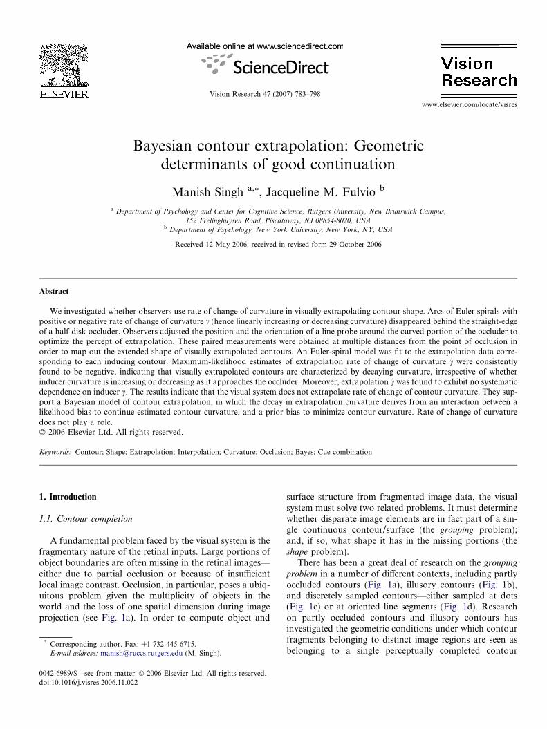
problem in a number of different contexts, including partlyoccluded contours (Fig. 1a), illusory contours (Fig. 1b),and discretely sampled contours—either sampled at dots(Fig. 1c) or at oriented line segments (Fig. 1d). Researchon partly occluded contours and illusory contours hasinvestigated the geometric conditions under which contourfragments belonging to distinct image regions are seen asbelonging to a single perceptually completed contour

a b

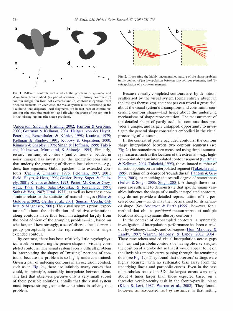
Fig. 2. Illustrating the highly unconstrained nature of the shape problemin the context of (a) interpolation between two contour segments, and (b)extrapolation of a contour segment.

Fig. 1. Different contexts within which the problems of grouping andshape have been studied: (a) partial occlusion, (b) illusory contours, (c)contour integration from dot elements, and (d) contour integration fromoriented elements. In each case, the visual system must determine (i) thelikelihood that disparate local fragments are in fact part of continuouscontour (the grouping problem), and (ii) what the shape of the contour isin the missing regions (the shape problem).

784 M. Singh, J.M. Fulvio / Vision Research 47 (2007) 783–798

(Anderson, Singh, & Fleming, 2002; Fantoni & Gerbino,2003; Guttman & Kellman, 2004; Heitger, von der Heydt,Peterhans, Rosenthaler, & Kubler, 1998; Kanizsa, 1979;Kellman & Shipley, 1991; Kubovy & Gepshtein, 2000;Ringach & Shapley, 1996; Singh & Hoffman, 1999; Takei-chi, Nakazawa, Murakami, & Shimojo, 1995). Similarly,research on sampled contours (and contours embedded innoisy images) has investigated the geometric constraintsthat underly the grouping of discrete local elements—e.g.,dots, line segments, Gabor patches—into extended con-tours (Caelli & Umansky, 1976; Feldman, 1997, 2001;Field, Hayes, & Hess, 1993; Geisler, Perry, Super, & Gallo-gly, 2001; Kovacs & Julesz, 1993; Pettet, McKee, & Grzy-wacz, 1998; Pizlo, Salach-Goyska, & Rosenfeld, 1997;Smits & Vos, 1987; Uttal, 1973), as well as how these con-straints relate to the statistics of natural images (Elder &Goldberg, 2002; Geisler et al., 2001; Sigman, Cecchi, Gil-bert, & Magnasco, 2001). The visual system’s prior ‘‘expec-tations’’ about the distribution of relative orientationsalong contours have thus been investigated largely fromthe point of view of the grouping problem—i.e., based onwhether, and how strongly, a set of discrete local elementsgroup perceptually into the representation of a singleextended contour.

By contrast, there has been relatively little psychophys-ical work on measuring the precise shapes of visually com-pleted contours. The visual system faces a difficult problemin interpolating the shapes of ‘‘missing’’ portions of con-tours, because the problem is so highly underconstrained:Given a pair of inducing contours in an occlusion context,such as in Fig. 2a, there are infinitely many curves thatcould, in principle, smoothly interpolate between them.The fact that observers perceive only a very small subsetof these possible solutions, entails that the visual systemmust impose strong geometric constraints in solving thisproblem.

Because visually completed contours are, by definition,synthesized by the visual system (being entirely absent inthe images themselves), their shapes can reveal a great dealabout the visual system’s assumptions and constraints con-cerning contour shape—and hence about the underlyingmechanisms of shape representation. The measurement ofthe detailed shape of partly occluded contours thus pro-vides a unique, and largely untapped, opportunity to inves-tigate the general shape constraints embodied in the visualprocessing of contours.

In the context of partly occluded contours, the contourshape interpolated between two contour segments (seeFig. 2a) has sometimes been measured using simple summa-ry measures, such as the location of the extremal—e.g., high-est—point along an interpolated contour segment (Guttman& Kellman, 2004; Takeichi, 1995), the estimated number ofinflection points on an interpolated segment (Takeichi et al.,1995), ratings of its degree of ‘roundedness’ (Fantoni & Ger-bino, 2003), or matching the overall degree of smoothness(Fulvio & Singh, 2006; Singh, 2004). Although these mea-sures are sufficient to demonstrate that specific image vari-ables influence the shape of visually interpolated contours,they do not provide a detailed representation of the per-ceived contour—which may then be analyzed for its extend-

ed shape. (See Anderson & Barth (1999), however, for amethod that obtains positional measurements at multiplelocations along a dynamic illusory contour.)

In the context of dot-sampled contours, a systematicinvestigation of interpolation performance has been carriedout by Maloney, Landy, and colleagues (Hon, Maloney, &Landy, 1997; Warren, Maloney, & Landy, 2002, 2004).These researchers studied visual interpolation across gapsin linear and parabolic contours by having observers adjustthe position of a probe dot so that it would appear to lie onthe (invisible) smooth curve passing through the remainingdots (see Fig. 1c). They found that observers’ settings werehighly accurate, with no systematic bias away from theunderlying linear and parabolic curves. Even in the caseof parabolas rotated in 3D, the largest errors were onlyabout 4 times larger than those expected based on athree-dot vernier-acuity task in the fronto-parallel plane(Klein & Levi, 1987; Warren et al., 2002). They found,however, an associated cost of curvature in that setting

M. Singh, J.M. Fulvio / Vision Research 47 (2007) 783–798 785

variability was significantly greater for the parabola thanfor the line. Finally, two of their results made it clear thatinterpolation performance is determined relatively locally:(1) increasing the number of dots beyond 4 (to 6 or 8)did not significantly improve performance (Warren et al.,2002), and (2) interpolation settings of the probe dot wereinfluenced only by the perturbation of the two nearest dotson each side; perturbing farther dots had hardly any influ-ence on the settings (Hon et al., 1997; Warren, Maloney, &Landy, 2004). This locality of the human visual spline isconsistent with Feldman’s (1997) hypothesis that the visualsystem analyzes sampled contours through local windowscontaining four consecutive dots each.

1.2. Shape constraints

The current study focuses on the context of contourextrapolation (see Fig. 2a). Extrapolation was taken as astarting point for a number of reasons. First, extrapolationis a critical component of the more general problem ofshape interpolation: an interpolating contour must bothsmoothly extrapolate each inducing contour, as well assmoothly connect the two extrapolants (Ullman, 1976;Fantoni & Gerbino, 2003). More importantly, extrapola-tion provides an ideal context within which to investigatethe geometric properties that the visual system uses incontinuing the shape of a contour. Specifically, our goalis to characterize the notion of ‘‘good continuation’’ of acontour in formal terms, by addressing the two followingquestions:

(1) What geometric properties (curvature, rate-of-changeof curvature, etc.) of a contour does the visual systemuse in extrapolating its shape?

(2) How does it use and combine these variables to definethe extended shape of a visually extrapolatedcontour?

Work in computational vision has proposed two shapeconstraints in solving the shape completion problem, thatbear on these questions. The first is that an interpolatingcontour must minimize the total curvature

Rj2 ds along

its length. This constraint has its roots in the theory of elas-ticity, where the total curvature is referred to as a curve’s‘‘bending energy’’ (Euler, 1744/1952; Love, 1927). Mini-mizing this energy leads to a class of curves known as elas-

tica—curves that are ‘‘as straight as possible’’ given theboundary conditions imposed by the physically specifiededges, and the requirement of smoothness. Elastica haveoften been used in computer vision for interpolating con-tours between pairs of contour segments (Horn, 1983;Mumford, 1994). The second constraint involves the mini-mization of variation in curvature

Rðdj

ds Þ2ds. Rather than

penalizing curvature per se, this constraint penalizes chang-

es in curvature (e.g., Barrow et al., 1981; Kimia, Frankel, &Popescu, 2003; Singh & Hoffman, 1999). As a result, thecontours tend locally toward being as close to circular as

the boundary conditions will allow, and generate a classof curves known as Euler spirals—characterized by a linearvariation in curvature as a function of arc length (Kimiaet al., 2003). There is indeed a history of work attributinga special status to circular arcs in contour interpolationand curve detection in noisy images. Ullman (1976), forinstance, modeled the shapes of illusory contours withthe combination of two circular arcs that respectivelyextrapolate the tangents of the two inducing contours,and meet with continuous tangents. In the context of curvedetection, Parent and Zucker (1989) introduced the notionof edge co-circularity—i.e., tangency to a common circle—and used it to compute the strength of grouping betweenoriented image elements. The closer two edges are to beingcocircular, the more strongly they are grouped.

The respective contributions of the above two con-straints in determining the extended shapes of contoursinterpolated by the visual system have, to our knowledge,not been investigated. There is, however, psychophysicalevidence for the instantiation of local versions of these con-straints in the context of discretely sampled contours. Inparticular, observers’ ability to visually integrate discretelocal elements into contours is found to deteriorate system-atically with increasing curvature—defined in terms of theturning angles between successive local elements (Feldman,1997; Field et al., 1993; Geisler et al., 2001; Pettet et al.,1998; Uttal, 1973). These results are consistent with an ‘‘as-sociation field’’ model in which the pattern of connectionstrengths between local orientation-tuned units is strongestwhen their preferred orientations are collinear, anddecreases monotonically with increasing turning angle(Field et al., 1993; Grossberg & Mingolla, 1985). This pat-tern of connection strengths is also found to be consistentwith the co-occurrence statistics of edge orientations alongextended contours in natural images (Elder & Goldberg,2002; Geisler et al., 2001). Similarly, there is evidence forthe local instantiation of minimization of variation in cur-vature in human contour perception. Observers’ perfor-mance in contour integration tasks is best when thevariance in the turning angles between successive local ele-ments is minimal (Feldman, 1997; Pizlo et al., 1997).Recent work on the statistics of natural images has alsofound that there is a prevalence of co-circular structure innatural images (Geisler et al., 2001; Sigman et al., 2001).Moreover, recent re-analysis of physiological data fromBosking, Zhang, and Fitzpatrick (1997) suggests that theassociation fields of individual orientation-tuned units inthe primary visual cortex may in fact be tuned to differentcurvatures—with the ‘‘standard’’ shape of the associationfield being a description of the population average, ratherthan of each individual unit (Ben-Shahar & Zucker, 2004).

The above two constraints are naturally viewed asembodying two different generative models of contours—expressed as different probability distributions on ‘‘succes-sive’’ orientations along contours. In discrete form, theminimization of curvature is locally consistent with a gen-erative model in which the position of the ‘‘next’’ point

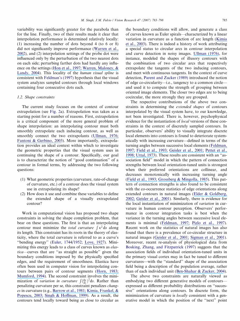
Fig. 4. Illustrating the role of occlusion in initiating mechanisms of visualcompletion (adapted from Bregman, 1981). The gray fragments areidentical in (a) and (b), but are more easily completed and recognized in(b).

786 M. Singh, J.M. Fulvio / Vision Research 47 (2007) 783–798

(in angular terms, measured from the current contourdirection) is characterized by a probability distribution cen-tered on a turning angle of a = 0 (i.e., ‘‘straight’’ is mostlikely) and falls off symmetrically with increasing magni-tude of a (see, e.g., Feldman, 1997; Feldman & Singh,2005; Yuille, Fang, Schrater, & Kersten, 2004). The mini-mization of variation in curvature, on the other hand, isconsistent with a generative model in which the positionof the next point is characterized by a probability distribu-tion centered on the previous turning angle (or a weightedaverage of the previous n turning angles)—so it tends tocontinue the estimated curvature of the contour.

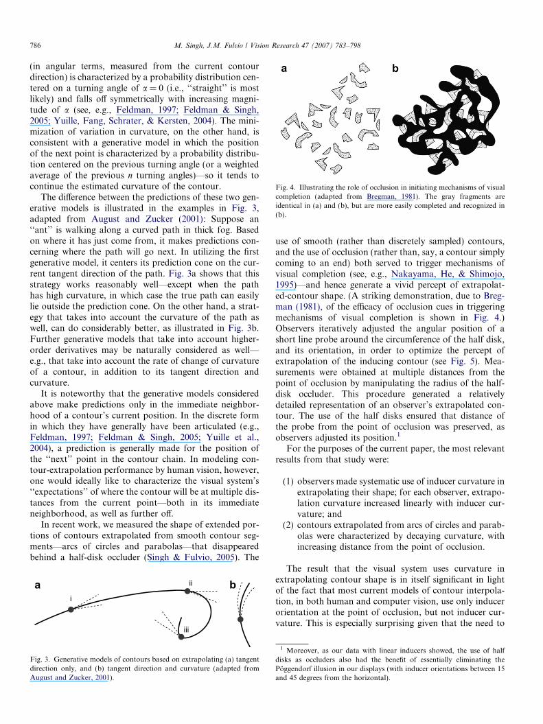
The difference between the predictions of these two gen-erative models is illustrated in the examples in Fig. 3,adapted from August and Zucker (2001): Suppose an‘‘ant’’ is walking along a curved path in thick fog. Basedon where it has just come from, it makes predictions con-cerning where the path will go next. In utilizing the firstgenerative model, it centers its prediction cone on the cur-rent tangent direction of the path. Fig. 3a shows that thisstrategy works reasonably well—except when the pathhas high curvature, in which case the true path can easilylie outside the prediction cone. On the other hand, a strat-egy that takes into account the curvature of the path aswell, can do considerably better, as illustrated in Fig. 3b.Further generative models that take into account higher-order derivatives may be naturally considered as well—e.g., that take into account the rate of change of curvatureof a contour, in addition to its tangent direction andcurvature.

It is noteworthy that the generative models consideredabove make predictions only in the immediate neighbor-hood of a contour’s current position. In the discrete formin which they have generally have been articulated (e.g.,Feldman, 1997; Feldman & Singh, 2005; Yuille et al.,2004), a prediction is generally made for the position ofthe ‘‘next’’ point in the contour chain. In modeling con-tour-extrapolation performance by human vision, however,one would ideally like to characterize the visual system’s‘‘expectations’’ of where the contour will be at multiple dis-tances from the current point—both in its immediateneighborhood, as well as further off.

In recent work, we measured the shape of extended por-tions of contours extrapolated from smooth contour seg-ments—arcs of circles and parabolas—that disappearedbehind a half-disk occluder (Singh & Fulvio, 2005). The

i

ii

iii

Fig. 3. Generative models of contours based on extrapolating (a) tangentdirection only, and (b) tangent direction and curvature (adapted fromAugust and Zucker, 2001).

use of smooth (rather than discretely sampled) contours,and the use of occlusion (rather than, say, a contour simplycoming to an end) both served to trigger mechanisms ofvisual completion (see, e.g., Nakayama, He, & Shimojo,1995)—and hence generate a vivid percept of extrapolat-ed-contour shape. (A striking demonstration, due to Breg-man (1981), of the efficacy of occlusion cues in triggeringmechanisms of visual completion is shown in Fig. 4.)Observers iteratively adjusted the angular position of ashort line probe around the circumference of the half disk,and its orientation, in order to optimize the percept ofextrapolation of the inducing contour (see Fig. 5). Mea-surements were obtained at multiple distances from thepoint of occlusion by manipulating the radius of the half-disk occluder. This procedure generated a relativelydetailed representation of an observer’s extrapolated con-tour. The use of the half disks ensured that distance ofthe probe from the point of occlusion was preserved, asobservers adjusted its position.1

For the purposes of the current paper, the most relevantresults from that study were:

(1) observers made systematic use of inducer curvature inextrapolating their shape; for each observer, extrapo-lation curvature increased linearly with inducer cur-vature; and

(2) contours extrapolated from arcs of circles and parab-olas were characterized by decaying curvature, withincreasing distance from the point of occlusion.

The result that the visual system uses curvature inextrapolating contour shape is in itself significant in lightof the fact that most current models of contour interpola-tion, in both human and computer vision, use only inducerorientation at the point of occlusion, but not inducer cur-vature. This is especially surprising given that the need to

1 Moreover, as our data with linear inducers showed, the use of halfdisks as occluders also had the benefit of essentially eliminating thePoggendorf illusion in our displays (with inducer orientations between 15and 45 degrees from the horizontal).

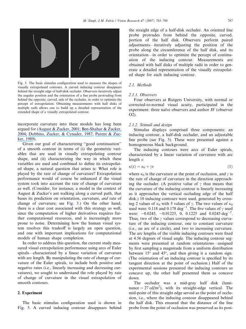
Fig. 5. The basic stimulus configuration used to measure the shapes ofvisually extrapolated contours. A curved inducing contour disappearsbehind the straight edge of half-disk occluder. Observers iteratively adjustthe angular position and the orientation of a line probe protruding frombehind the opposite, curved, side of the occluder, in order to optimize thepercept of extrapolation. Obtaining measurements with half disks ofmultiple radii allows one to build up a detailed representation of theextended shape of a visually extrapolated contour.

M. Singh, J.M. Fulvio / Vision Research 47 (2007) 783–798 787

incorporate curvature into these models has long beenargued for (August & Zucker, 2001; Ben-Shahar & Zucker,2004; Dobbins, Zucker, & Cynader, 1987; Parent & Zuc-ker, 1989).

Given our goal of characterizing ‘‘good continuation’’of a smooth contour in terms of (i) the geometric vari-ables that are used in visually extrapolating contourshape, and (ii) characterizing the way in which thesevariables are used and combined to define its extrapolat-ed shape, a natural question that arises is: What role isplayed by the rate of change of curvature? Extrapolationperformance would of course be enhanced if the visualsystem took into account the rate of change of curvatureas well. (Consider, for instance, a model in the context ofAugust & Zucker’s ant walking along a curved path, thatbases its prediction on orientation, curvature, and rate ofchange of curvature; see Fig. 3.) On the other hand,there is a clear cost associated with this strategy as well,since the computation of higher derivatives requires fur-ther computational resources, and is increasingly moreprone to noise. Determining how the human visual sys-tem resolves this tradeoff is largely an open question,and one with important implications for computationalmodels of human shape completion.

In order to address this question, the current study mea-sured visual extrapolation performance using arcs of Eulerspirals—characterized by a linear variation of curvaturewith arc length. By manipulating the rate of change of cur-vature of the Euler spirals, to include both positive andnegative rates (i.e., linearly increasing and decreasing cur-vatures), we sought to understand the role played by rateof change of curvature in the visual extrapolation ofsmooth contours.

2. Experiment

The basic stimulus configuration used is shown inFig. 5. A curved inducing contour disappears behind

the straight edge of a half-disk occluder. An oriented lineprobe protrudes from behind the opposite, curved,portion of the half disk. Observers perform pairedadjustments—iteratively adjusting the position of theprobe along the circumference of the half disk, and itsorientation—in order to optimize the percept of continu-ation of the inducing contour. Measurements areobtained with half disks of multiple radii in order to gen-erate a detailed representation of the visually extrapolat-ed shape for each inducing contour.

2.1. Methods

2.1.1. Observers

Four observers at Rutgers University, with normal orcorrected-to-normal visual acuity, participated in theexperiment: three naıve observers and author JF (observerO2).

2.1.2. Stimuli and design

Stimulus displays comprised three components: aninducing contour, a half-disk occluder, and an adjustableline probe (see Fig. 5). These were presented against ahomogeneous black background.

The inducing contours were arcs of Euler spirals,characterized by a linear variation of curvature with arclength s:

jðsÞ ¼ j0 þ cs ð1Þ

where j0 is the curvature at the point of occlusion, and c isthe rate of change of curvature in the direction approach-ing the occluder. (A positive value of c thus means thatthe curvature of the inducing contour is linearly increasingas it approaches the vertical occluding edge of the halfdisk.) 10 inducing contours were used, generated by cross-ing 2 values of j0 with 5 values of c. The two values of j0

used were: 0.118 and 0.178 deg�1. The five values of c usedwere: �0.0245, �0.01225, 0, 0.1225 and 0.0245 deg�2.Thus, two of the c values correspond to decreasing curva-ture of the inducing contour, one to constant curvature(i.e., an arc of a circle), and two to increasing curvature.The arc lengths of the visible inducing contours were fixedat 4.56 degrees of visual angle. The inducing contour seg-ments were presented at random orientations—assignedby first sampling a magnitude from a uniform distributionbetween 15� and 45�, and then giving it a random sign.(The orientation of an inducing contour is specified by itstangent direction at the point of occlusion.) Half of theexperimental sessions presented the inducing contours asconcave up, the other half presented them as concavedown.

The occluder was a mid-gray half disk (lumi-nance = 27 cd/m2), with its straight-edge vertical. Themid-point of this straight edge served as the point of occlu-sion, i.e., where the inducing contour disappeared behindthe half disk. This ensured that the distance of the lineprobe from the point of occlusion was preserved as its posi-

θ∗

ϕ∗

θ

ϕ

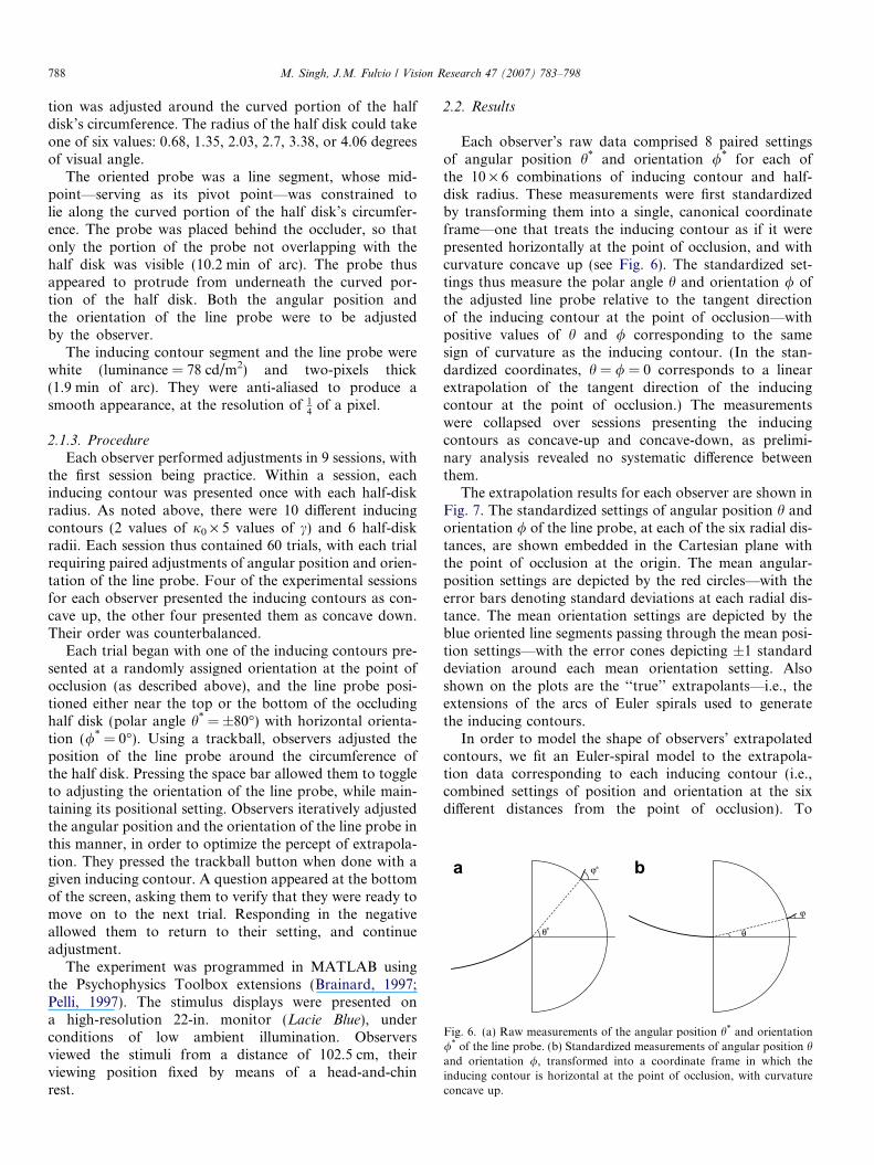
Fig. 6. (a) Raw measurements of the angular position h* and orientation/* of the line probe. (b) Standardized measurements of angular position hand orientation /, transformed into a coordinate frame in which theinducing contour is horizontal at the point of occlusion, with curvatureconcave up.

788 M. Singh, J.M. Fulvio / Vision Research 47 (2007) 783–798

tion was adjusted around the curved portion of the halfdisk’s circumference. The radius of the half disk could takeone of six values: 0.68, 1.35, 2.03, 2.7, 3.38, or 4.06 degreesof visual angle.

The oriented probe was a line segment, whose mid-point—serving as its pivot point—was constrained tolie along the curved portion of the half disk’s circumfer-ence. The probe was placed behind the occluder, so thatonly the portion of the probe not overlapping with thehalf disk was visible (10.2 min of arc). The probe thusappeared to protrude from underneath the curved por-tion of the half disk. Both the angular position andthe orientation of the line probe were to be adjustedby the observer.

The inducing contour segment and the line probe werewhite (luminance = 78 cd/m2) and two-pixels thick(1.9 min of arc). They were anti-aliased to produce asmooth appearance, at the resolution of 1

4of a pixel.

2.1.3. Procedure

Each observer performed adjustments in 9 sessions, withthe first session being practice. Within a session, eachinducing contour was presented once with each half-diskradius. As noted above, there were 10 different inducingcontours (2 values of j0 · 5 values of c) and 6 half-diskradii. Each session thus contained 60 trials, with each trialrequiring paired adjustments of angular position and orien-tation of the line probe. Four of the experimental sessionsfor each observer presented the inducing contours as con-cave up, the other four presented them as concave down.Their order was counterbalanced.

Each trial began with one of the inducing contours pre-sented at a randomly assigned orientation at the point ofocclusion (as described above), and the line probe posi-tioned either near the top or the bottom of the occludinghalf disk (polar angle h* = ±80�) with horizontal orienta-tion (/* = 0�). Using a trackball, observers adjusted theposition of the line probe around the circumference ofthe half disk. Pressing the space bar allowed them to toggleto adjusting the orientation of the line probe, while main-taining its positional setting. Observers iteratively adjustedthe angular position and the orientation of the line probe inthis manner, in order to optimize the percept of extrapola-tion. They pressed the trackball button when done with agiven inducing contour. A question appeared at the bottomof the screen, asking them to verify that they were ready tomove on to the next trial. Responding in the negativeallowed them to return to their setting, and continueadjustment.

The experiment was programmed in MATLAB usingthe Psychophysics Toolbox extensions (Brainard, 1997;Pelli, 1997). The stimulus displays were presented ona high-resolution 22-in. monitor (Lacie Blue), underconditions of low ambient illumination. Observersviewed the stimuli from a distance of 102.5 cm, theirviewing position fixed by means of a head-and-chinrest.

2.2. Results

Each observer’s raw data comprised 8 paired settingsof angular position h* and orientation /* for each ofthe 10 · 6 combinations of inducing contour and half-disk radius. These measurements were first standardizedby transforming them into a single, canonical coordinateframe—one that treats the inducing contour as if it werepresented horizontally at the point of occlusion, and withcurvature concave up (see Fig. 6). The standardized set-tings thus measure the polar angle h and orientation / ofthe adjusted line probe relative to the tangent directionof the inducing contour at the point of occlusion—withpositive values of h and / corresponding to the samesign of curvature as the inducing contour. (In the stan-dardized coordinates, h = / = 0 corresponds to a linearextrapolation of the tangent direction of the inducingcontour at the point of occlusion.) The measurementswere collapsed over sessions presenting the inducingcontours as concave-up and concave-down, as prelimi-nary analysis revealed no systematic difference betweenthem.

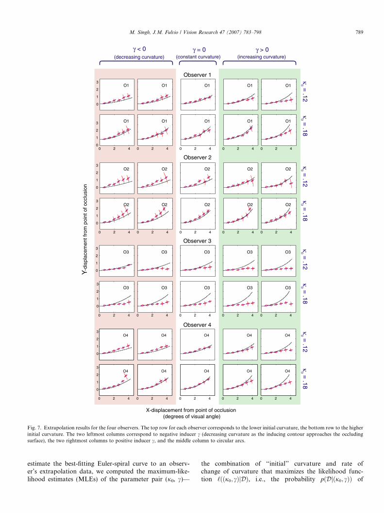
The extrapolation results for each observer are shown inFig. 7. The standardized settings of angular position h andorientation / of the line probe, at each of the six radial dis-tances, are shown embedded in the Cartesian plane withthe point of occlusion at the origin. The mean angular-position settings are depicted by the red circles—with theerror bars denoting standard deviations at each radial dis-tance. The mean orientation settings are depicted by theblue oriented line segments passing through the mean posi-tion settings—with the error cones depicting ±1 standarddeviation around each mean orientation setting. Alsoshown on the plots are the ‘‘true’’ extrapolants—i.e., theextensions of the arcs of Euler spirals used to generatethe inducing contours.

In order to model the shape of observers’ extrapolatedcontours, we fit an Euler-spiral model to the extrapola-tion data corresponding to each inducing contour (i.e.,combined settings of position and orientation at the sixdifferent distances from the point of occlusion). To

γ < 0(decreasing curvature)

γ = 0(constant curvature)

γ > 0(increasing curvature)

0

1

2

3O1 O1 O1 O1 O1

0

1

2

3

0 2 4

O1

0 2 4

O1

0 2 4

O1

0 2 4

O1

0 2 4

O1

0

1

2

3O2 O2 O2 O2 O2

0 2 4

0

1

2

3O2

0 2 4

O2

0 2 4

O2

0 2 4

O2

0 2 4

O2

X-displacement from point of occlusion(degrees of visual angle)

Y-di

spla

cem

ent f

rom

poi

nt o

f occ

lusi

on

Observer 1

Observer 2

κ0 =

.12κ

0 = .18

κ0 =

.12κ

0 = .18

κ0 =

.12κ

0 = .18

κ0 =

.12κ

0 = .18

Observer 3

Observer 4

0

1

2

3O3 O3 O3 O3 O3

0 2 4

0

1

2

3O3

0 2 4

O3

0 2 4

O3

0 2 4

O3

0 2 4

O3

0

1

2

3O4 O4 O4 O4 O4

0 2 4

0

1

2

3O4

0 2 4

O4

0 2 4

O4

0 2 4

O4

0 2 4

O4

Fig. 7. Extrapolation results for the four observers. The top row for each observer corresponds to the lower initial curvature, the bottom row to the higherinitial curvature. The two leftmost columns correspond to negative inducer c (decreasing curvature as the inducing contour approaches the occludingsurface), the two rightmost columns to positive inducer c, and the middle column to circular arcs.

M. Singh, J.M. Fulvio / Vision Research 47 (2007) 783–798 789

estimate the best-fitting Euler-spiral curve to an observ-er’s extrapolation data, we computed the maximum-like-lihood estimates (MLEs) of the parameter pair (j0, c)—

the combination of ‘‘initial’’ curvature and rate ofchange of curvature that maximizes the likelihood func-tion ‘ððj0; cÞjDÞ, i.e., the probability pðDjðj0; cÞÞ of

0.1 0.2 0.3

–0.08

–0.06

–0.04

–0.02

0

0.02 O1

0.1 0.2 0.3

–0.08

–0.06

–0.04

–0.02

0

0.02 O2

0.1 0.2 0.3

–0.1

–0.05

0O3

0.1 0.2 0.3

–0.08

–0.06

–0.04

–0.02

0

0.02 O4

Initial Curvature (deg-1)

Rat

e of

cha

nge

of c

urva

ture

(de

g-2)

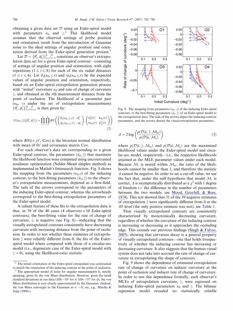
Fig. 8. The mapping from parameters (j0, c) of the inducing Euler-spiralcontours, to the best-fitting parameters ðj0; cÞ of an Euler-spiral model tothe extrapolation data. The tails of the arrows depict the inducing-contourparameters, and the arrows denote the visual-extrapolation parameters.

790 M. Singh, J.M. Fulvio / Vision Research 47 (2007) 783–798

obtaining a given data set D using an Euler-spiral modelwith parameters j0 and c.2 This likelihood modelassumes that the observed settings of probe positionand orientation result from the introduction of Gaussiannoise to the ideal settings of angular position and orien-tation derived from the Euler-spiral generation process.3

Let D ¼ fhir;/

irgj

8i¼1j

6r¼1 constitute an observer’s extrapo-

lation data set for a given Euler-spiral contour—consistingof settings of angular position and orientation, with eightrepetitions (1 6 i 6 8) for each of the six radial distances(1 6 r 6 6). Let he(j0,c, r) and /e(j0,c, r) be the expectedvalues of angular position and orientation, respectively,based on an Euler-spiral extrapolation generation processwith ‘‘initial’’ curvature j0 and rate of change of curvaturec, and obtained at the rth measurement distance from thepoint of occlusion. The likelihood of a parameter pair(j0, c) under the set of extrapolation measurementsfhi

r;/irgj

8i¼1j

6r¼1 is then given by:

‘ððj0;cÞjfhir;/

irgÞ¼

Y6

r¼1

Y8

i¼1

BNheðj0;c;rÞ�hi

r

/eðj0;c;rÞ�/ir

!;

r2hðrÞ rh/ðrÞ

rh/ðrÞ r2/ðrÞ

! !

ð2Þ

where BN((x y) 0, Cov) is the bivariate normal distributionwith mean (0 0) 0 and covariance matrix Cov.

For each observer’s data set corresponding to a givenEuler-spiral contour, the parameters ðj0; cÞ that maximizethe likelihood function were computed using unconstrainednonlinear optimization (Nelder-Mead simplex method) asimplemented in Matlab’s fminsearch function. Fig. 8 showsthe mapping from the parameters (j0,c) of the inducingcontour, to the best-fitting parameters ðj0; cÞ to the observ-er’s extrapolation measurements, depicted as a flow-field.The tails of the arrows correspond to the parameters ofthe inducing Euler-spiral contour, whereas the arrowheadscorrespond to the best-fitting extrapolation parameters ofthe Euler-spiral model.

A salient feature of these fits to the extrapolation data isthat, in 39 of the 40 cases (4 observers · 10 Euler-spiralcontours), the best-fitting value for the rate of change ofcurvature, c, is negative (see Fig. 8)—indicating that thevisually extrapolated contours consistently have decreasingcurvature with increasing distance from the point of occlu-sion. In order to test whether these estimates of extrapola-tion c were reliably different from 0, the fits of the Euler-spiral model where compared with those of a circular-arcmodel (i.e., degenerate case of the Euler-spiral model withc = 0), using the likelihood-ratio statistic:

2 The initial orientation of the Euler-spiral extrapolant was constrainedto match the orientation of the inducing contour at the point of occlusion.

3 The appropriate model of noise for angular measurements is, strictlyspeaking, given by the von Mises distribution. However, given the smallstandard deviations in our data (SDs <10� for h, SDs <15� for /), the vonMises distribution is very closely approximated by the Gaussian. (Indeed,the von Mises converges to the Gaussian as r! 0; see, e.g., Mardia &Jupp (2000).)

D ¼ 2 logpðDjj; c;MesÞ

pðDjj;McÞ

� �ð3Þ

where pðDjj; c;MesÞ and pðDjj;McÞ are the maximizedlikelihood values under the Euler-spiral model and circu-lar-arc model, respectively—i.e., the respective likelihoodsattained at the MLE parameter values under each model.Because Mc is nested within Mes, the ratio of the likeli-hoods cannot be smaller than 1, and therefore the statisticD cannot be negative. In order to set a cut-off value, we usethe fact that, under the null hypothesis that model Mc iscorrect, D is asymptotically distributed as a v2 with 1 degreeof freedom (= the difference in the number of parametersbetween the two models; see Mood, Graybill, & Boes,1974). This test showed that 31 of the 39 negative estimatesof extrapolation c were significantly different from 0 at the.05 level (the only positive estimate was not); see Table 1.

Thus visually extrapolated contours are consistentlycharacterized by monotonically decreasing curvature,regardless of whether the curvature of the inducing contouris increasing or decreasing as it approaches the occludingedge. This extends our previous findings (Singh & Fulvio,2005), showing that curvature decay is a general propertyof visually extrapolated contours—one that holds irrespec-tively of whether the inducing contour has increasing ordecreasing curvature. It also suggests that the human visualsystem does not take into account the rate of change of cur-vature in extrapolating the shape of contours.

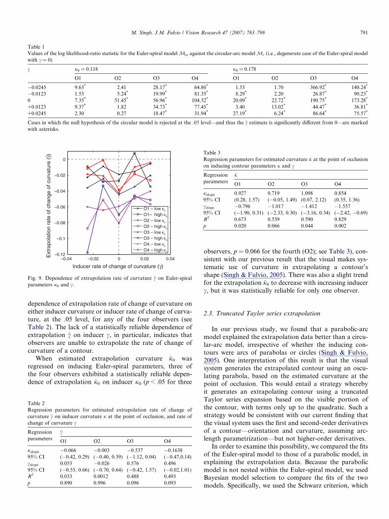
Fig. 9 shows the dependence of estimated extrapolationrate of change of curvature on inducer curvature at thepoint of occlusion and inducer rate of change of curvature.In order to test this dependence formally, each observer’sMLEs of extrapolation curvature, c, were regressed oninducing Euler-spiral parameters j0 and c. The bilinearregression model revealed no statistically reliable

Table 1Values of the log likelihood-ratio statistic for the Euler-spiral model Mes against the circular-arc model Mc (i.e., degenerate case of the Euler-spiral modelwith c = 0)

c j0 = 0.118 j0 = 0.178

O1 O2 O3 O4 O1 O2 O3 O4

�0.0245 9.63* 2.41 28.17* 64.80* 1.53 1.70 366.92* 140.24*

�0.0123 1.53 5.24* 19.99* 81.35* 8.29* 2.20 26.87* 90.23*

0 7.35* 51.45* 56.96* 104.32* 20.09* 22.72* 190.75* 173.28*

+0.0123 9.37* 1.82 34.73* 77.45* 3.40 13.02* 44.47* 36.81*

+0.0245 2.30 0.27 18.47* 31.94* 27.19* 6.24* 86.64* 75.57*

Cases in which the null hypothesis of the circular model is rejected at the .05 level—and thus the c estimate is significantly different from 0—are markedwith asterisks.

–0.04 –0.02 0 0.02 0.04–0.12

–0.1

–0.08

–0.06

–0.04

–0.02

0

O1 – low κ0

O1– high κ0

O2 – low κ0

O2 – high κ0

O3 – low κ0

O3 – high κ0

O4 – low κ0

O4 – high κ0

Inducer rate of change of curvature (γ)

Ext

rapo

latio

n ra

te o

f cha

nge

of c

urva

ture

(γ)

Fig. 9. Dependence of extrapolation rate of curvature c on Euler-spiralparameters j0 and c.

Table 3Regression parameters for estimated curvature j at the point of occlusionon inducing contour parameters j and c

Regressionparameters

j

O1 O2 O3 O4

jslope 0.927 0.719 1.098 0.85495% CI (0.28, 1.57) (�0.05, 1.49) (0.07, 2.12) (0.35, 1.36)cslope �0.796 �1.017 �1.412 �1.55795% CI (�1.90, 0.31) (�2.33, 0.30) (�3.16, 0.34) (�2.42, �0.69)R2 0.673 0.539 0.590 0.829p 0.020 0.066 0.044 0.002

M. Singh, J.M. Fulvio / Vision Research 47 (2007) 783–798 791

dependence of extrapolation rate of change of curvature oneither inducer curvature or inducer rate of change of curva-ture, at the .05 level, for any of the four observers (seeTable 2). The lack of a statistically reliable dependence ofextrapolation c on inducer c, in particular, indicates thatobservers are unable to extrapolate the rate of change ofcurvature of a contour.

When estimated extrapolation curvature j0 wasregressed on inducing Euler-spiral parameters, three ofthe four observers exhibited a statistically reliable depen-dence of extrapolation j0 on inducer j0 (p < .05 for three

Table 2Regression parameters for estimated extrapolation rate of change ofcurvature c on inducer curvature j at the point of occlusion, and rate ofchange of curvature c

Regressionparameters

c

O1 O2 O3 O4

jslope �0.066 �0.003 �0.537 �0.163895% CI (�0.42, 0.29) (�0.40, 0.39) (�1.12, 0.04) (�0.47,0.14)cslope 0.053 �0.026 0.576 0.49695% CI (�0.55, 0.66) (�0.70, 0.64) (�0.42, 1.57) (�0.02,1.01)R2 0.033 0.0012 0.488 0.493p 0.890 0.996 0.096 0.093

observers, p = 0.066 for the fourth (O2); see Table 3), con-sistent with our previous result that the visual makes sys-tematic use of curvature in extrapolating a contour’sshape (Singh & Fulvio, 2005). There was also a slight trendfor the extrapolation j0 to decrease with increasing inducerc, but it was statistically reliable for only one observer.

2.3. Truncated Taylor series extrapolation

In our previous study, we found that a parabolic-arcmodel explained the extrapolation data better than a circu-lar-arc model, irrespective of whether the inducing con-tours were arcs of parabolas or circles (Singh & Fulvio,2005). One interpretation of this result is that the visualsystem generates the extrapolated contour using an oscu-lating parabola, based on the estimated curvature at thepoint of occlusion. This would entail a strategy wherebyit generates an extrapolating contour using a truncatedTaylor series expansion based on the visible portion ofthe contour, with terms only up to the quadratic. Such astrategy would be consistent with our current finding thatthe visual system uses the first and second-order derivativesof a contour—orientation and curvature, assuming arc-length parametrization—but not higher-order derivatives.

In order to examine this possibility, we compared the fitsof the Euler-spiral model to those of a parabolic model, inexplaining the extrapolation data. Because the parabolicmodel is not nested within the Euler-spiral model, we usedBayesian model selection to compare the fits of the twomodels. Specifically, we used the Schwarz criterion, which

Table 4Schwarz-criterion values for the Euler-spiral model Mes against the parabolic model Mp

c j0 = 0.118 j0 = 0.178

O1 O2 O3 O4 O1 O2 O3 O4

�0.0245 �1.51 3.82* 9.78* 20.91* 0.94* 18.16* 155.55* 26.82*

�0.0123 �0.79 2.14* 7.29* 28.65* �2.03 16.52* 9.94* 15.81*

0 �1.55 �2.28 23.80* 39.75* 1.35* 1.36* 82.06* 50.06*

+0.0123 �1.22 1.13* 14.78* 32.03* 15.29* 31.61* 17.85* 5.68*

+0.0245 �1.47 �1.81 6.70* 12.18* 0.94* �0.62* 39.87* 25.48*

Cases in which the increase in the goodness of fit of the Euler-spiral model is sufficiently high to offset its additional parameter, are indicated by positivevalues (marked with asterisks).

792 M. Singh, J.M. Fulvio / Vision Research 47 (2007) 783–798

provides an asymptotic approximation to the logarithm ofthe Bayes factor, i.e., the ratio of marginal likelihoodspðDjMesÞ=pðDjMpÞ under the two models (see Kass &Raftery, 1995; Schwarz, 1978). The Schwarz criterion isgiven by:

S ¼ logpðDjj0; c;MesÞ

pðDjj0;MpÞ

� �� 1

2ðkes � kpÞ logðNÞ ð4Þ

where pðDjj0; c;MesÞ and pðDjj0;MpÞ are respectively themaximized likelihood values under the two models (thelikelihoods corresponding to the MLE parameter values),kes and kp are their respective numbers of parameters (2for the Euler-spiral model, 1 for the parabolic model),and N is sample size (=96, since each observer makes 48settings of h, and 48 settings of / for each contour).4 Inthe above expression, the first term captures the relativegoodness of fit of the two models to the data, whereasthe second term constitutes a penalty for more complexmodels (i.e., with more parameters). The fits to the para-bolic model were determined using a likelihood functionwith the same functional form as Eq. (2), but with the ‘‘ex-pected’’ angular positions hp(j0, r) and orientations/p(j0, r) at various radial distances r based on a parabolawith curvature j0 at its vertex (the point of occlusion).

The Schwarz-criterion test showed that the Euler-spiralmodel was superior to the parabolic model in 31 of the40 cases (see Table 4)—thereby indicating that visuallyextrapolated shape is not best characterized by a parabolicmodel (or, equivalently, a Taylor series truncated beyondthe quadratic term). Specifically, in a large majority ofthe cases, the increase in the fit to the data was sufficientlyhigh to warrant the additional parameter of the Euler-spiral model. Indeed, a comparison of the logarithmic-spiral model to the Euler-sprial model using the Schwarzcriterion revealed the log-spiral model to be superior in29 of the 40 cases.5 The superior fits of the log-spiral modelare consistent with our previous findings (Singh & Fulvio,2005), and indicate that a nonlinear decrease in curvature,

4 The Schwarz criterion is closely related to the Bayes InformationCriterion (BIC); in fact, it equals twice the difference between therespective BIC values of the two models (see, e.g., Kass & Raftery, 1995).

5 A lograrithmic spiral is characterized by the intrinsic Cesaro equationjðsÞ ¼ 1

aþbs, so its curvature j varies inversely with its arc length s.

asymptoting to 0, better characterizes the shape of visuallyextrapolated contours than a linear decrease.

2.3.1. Scale invariance vs. short/long-range dichotomy

Our analysis has assumed that the same model ofextrapolation applies for the entire range of distances test-ed, i.e., at all scales of interest—hence, scale invariance.Another possibility, however, is that there may be a princi-pled distinction between ‘short-range’ and ‘long-range’ dis-tances from the point of occlusion. Based in part onpsychophyiscal results on the perception of contours indot-sampled stimuli, Zucker and colleagues have proposedthat two distinct stages are involved in the inference of con-tours from groups of discrete dots or line segments (seeLink & Zucker, 1988; Zucker & Davis, 1988; Zucker, Dob-bins, & Iverson, 1989). The first stage, operating over a rel-atively short range, includes receptive-field-basedconvolutions responsible for computing local orientationsignals (represented coarsely at this stage), as well as localinteractions between these convolutions, based on co-circu-larity. The second stage, operating over a larger range, isresponsible for the inference of the global structure of thecontour.

This account raises the possibility that different shapeconstraints may operate in contour extrapolation depend-ing on whether they involve ‘short range’ or ‘long range’interactions. It is possible, for instance, that the extrapo-lant shape may be based on co-circularity (i.e., constant-curvature extrapolation) at small distances from the pointof occlusion, and the decaying curvature behavior obtainsonly at larger distances. Unfortunately, it is impossible toreliably distinguish between this hypothesis and a scale-in-variant hypothesis from our data. If we restrict ourselves tothe smallest measurement distance (0.68 deg)—or even thesmallest two measurement distances (0.68 and 1.35 deg)—used in our experiment, the predictions of a circular-arcmodel and those of an Euler-spiral model are statisticallyindistinguishable for our stimuli. The largest differencesin predicted angular position (obtained for the highestmagnitude of rate of change of curvature;jcj = 0.0245 deg�2) are 0.11� and 0.43� for the first twomeasurement distances (with the corresponding differencesin predicted orientation being 0.33� and 1.3�, respectively).It is only by including the larger measurement distances, as

–1 0 10

0.2

0.4

0.6

0.8

1

O11

–1 0 10

0.2

0.4

0.6

0.8

1

O12

Pro

port

ion

"incr

easi

ng c

urva

ture

" re

spon

ses

–1 0 10

0.2

0.4

0.6

0.8

1

O13

Rate of change of curvature γ

(x 10 )–5

deg–2

κ0 = 0.118 deg -1

κ0 = 0.178 deg -1

Fig. 10. Results in the task involving the detection of variation incurvature. The data indicate that observers can reliably identify whetherthe curvature of the inducing contour is increasing or decreasing; hencethe failure to extrapolate rate of change of curvature does not simplyreflect observers’ inability to detect it.

M. Singh, J.M. Fulvio / Vision Research 47 (2007) 783–798 793

we did in the main analyses reported above, that the predic-tions of alternative models can be reliably distinguished inour data. Testing for the possible manifestation of a short-range vs. long-range distinction in the context of contourextrapolation will thus require future measurements thatare aimed directly at distinguishing between a circular-arcmodel and an Euler-spiral model (or some other model thatcan exhibit a decrease in curvature) at very short distancesfrom the point of occlusion.

2.4. Detection of variation in curvature

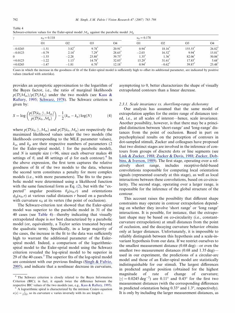
The above analyses show that observers did not use therate of change of curvature in extrapolating contour shape.Moreover, their visually extrapolated contours were consis-tently characterized by decreasing curvature, irrespective ofwhether the inducer curvature was increasing or decreasingas it approached the occluder. Do these results simplyreflect the fact that observers were unable to detect the var-iation in curvature along the inducing contours used (i.e.,for the particular combinations of curvature, rate ofchange of curvature, and arc length of the inducing con-tours used in the experiment)?

In order to address this question, we obtained addi-tional measurements on three naıve observers. We usedthe same 10 arcs of Euler spirals as in the main experi-ment (2 values of curvature · 5 values of rate of changeof curvature), with the same fixed arc length of 4.56 deg.Unlike the main experiment, however, the stimulus didnot include an adjustable line probe. Observers simplyindicated whether the curvature of the inducing contourwas increasing or decreasing as it approaches the occlu-der. The occluder size was not manipulated; its radiuswas fixed at 2.03 deg (half of the largest radius used inthe main experiment).

Each observer participated in five sessions, with the firstone being practice. The inducing contour was presented ata randomly assigned orientation, as in the main experi-ment. Two of the experimental sessions presented the con-tour as concave up, the other two as concave down, withtheir order counterbalanced. Each session contained 240trials, with each trial requiring a 2AFC response of ‘‘in-creasing’’ or ‘‘decreasing’’ curvature. Each observer thusran a total of 960 experimental trials.

Fig. 10 plots the data for the three observers. Each datapoint corresponds to the mean of 96 trials, for a giveninducing contour (i.e., a particular combination of curva-ture and rate of change of curvature). Also shown on theplots are the fits of Weibull functions to the data (Wich-mann & Hill, 2001). Although a small bias is apparent insome cases, it is evident that all observers are able to distin-guish perceptually between increasing and decreasing cur-vature on the inducing contours. Thus the failure to usevariation in curvature in extrapolating contours cannotbe attributed to a failure to detect the variation in curva-ture in the inducing contours used. (Note, in particular,that observers’ performance in detecting the positive rate

of change of curvature is consistently high for the largervalue of c used. Hence, the observed property of decreasingcurvature of visually extrapolated contours cannot be dueto a misperception of the sign of variation in curvatureof the inducing contours.)

3. Bayesian contour extrapolation

Our results indicate that human observers do not use therate of change of curvature in extrapolating contour shape.Visually extrapolated contours are consistently character-ized by decaying curvature, regardless of whether theinducing contours have increasing or decreasing curvature.Furthermore, extrapolation rate of change of curvature

794 M. Singh, J.M. Fulvio / Vision Research 47 (2007) 783–798

exhibits no systematic dependence on the rate of change ofcurvature of the inducing contours. These results thus spec-ify clear limits on the geometric properties that the visualsystem uses in ‘‘continuing’’ the shape of a contour: it usestangent direction and curvature, but not rate of change ofcurvature.

These results also provide further support for a Bayesianmodel outlined by Singh and Fulvio (2005)—which isbased on an interaction between the tendency to minimizecurvature and the tendency to continue estimated curva-ture. The prior and the likelihood in the model areexpressed as probability distributions on extrapolation cur-vature jext. The prior captures the default expectation ofthe visual system—in the absence of any other informa-tion—that a contour will simply ‘‘go straight’’ (Elder &Goldberg, 2002; Feldman, 1997; Field et al., 1993; Geisleret al., 2001; Yuille et al., 2004), and is expressed as a Gauss-ian distribution on extrapolation curvature, centered on 0:

pðjextÞ � Nð0; rprÞ ð5Þ

for some rpr. This bias is consistent in spirit with approach-es that minimize total curvature along the length of thecontour (Horn, 1983; Mumford, 1994), but is expressedas a probability distribution on local curvature. The likeli-hood bias captures the tendency toward co-circularity,namely, the tendency to ‘‘continue’’ the curvature of theinducing contour estimated at the point of occlusion (Elder& Goldberg, 2002; Feldman, 1997; Geisler et al., 2001; Par-ent & Zucker, 1989; Pizlo et al., 1997). It is consistent inspirit with approaches that minimize variation in curvature(Kimia et al., 2003), except that it takes into account thecurvature of the inducing contour as well,6 and is expressedas a distribution on local extrapolation curvature (centeredon the estimated inducer curvature ji at the point of occlu-sion). A key component of the model is the assumptionthat the continuation of inducer curvature is subject to sys-tematically greater variability, with increasing distancefrom the point of occlusion. Specifically, a Weber-likedependence is assumed, such that the standard deviationincreases linearly with distance d from the point of occlu-sion: rlikðdÞ ¼ r0

lik þ md, where r0lik is the standard devia-

tion when the gap size is zero (infinitesimally thinoccluder). The likelihood function is thus given by:

‘ðjextjji; dÞ � Nðji; r0lik þ mdÞ ð6Þ

The two constraints articulated above serve as probabilisticbiases, or cues, to visual extrapolation. Their combination,via Bayes’ Theorem, is given by:

6 Consistent with the general calculus-of-variations approach to contourinterpolation (e.g., Horn, 1983; Mumford, 1994), approaches based onminimizing variation in curvature (e.g., Kimia et al., 2003) obtain the totalvalue of curvature variation by integrating only over the interpolatedportion of the contour—not including the physically specified inducingcontours. As a result, although the interpolated portion of the contour issecond-order smooth, curvature discontinuities are generally introduced atpoints where the interpolated contour meets the inducing contours.

pðjextjji; dÞ ¼‘ðjextjji; dÞ � pðjextÞ

pðjiÞð7Þ

Under the assumption that the prior and likelihoods areboth Gaussian distributions, there exist standard formulasfor the posterior (Box & Tiao, 1992). In particular, the pos-terior is also a Gaussian with mean and variance given by:

lpostðji; dÞ¼lpr

r2pr

þ llik

r2likðji; dÞ

!,1

r2pr

þ 1

r2likðji; dÞ

!

r2postðji; dÞ ¼ 1

1

r2pr

þ 1

r2likðji; dÞ

!,ð8Þ

Interpreting these two biases or cues strictly as prior andlikelihood is in fact not necessary. Treating the two distri-butions as probabilistic cues, or sources of information, thetheory of cue combination (or sensor fusion) gives the sameexpression for optimal combination (see Singh & Fulvio,2006). Specifically, the optimal combination of two sto-chastic signals (in the statistical sense of a minimum-vari-ance unbiased estimator) is given by a weighted averageof their expected values, with the weights being proportion-al to their respective reliabilities (i.e., reciprocals of theirvariances; see, e.g., Clark & Yuille, 1990; Landy, Maloney,Johnston, & Young, 1995). Thus, consistent with theexpression for the expected extrapolation curvature above:

jextðdÞ ¼ wpr � lpr þ wlik � llik ð9Þ

where wpr / 1=r2pr and wlik / 1=r2

lik.Under the natural assumption that the continuation of

estimated inducer curvature is subject to very little noiseat the point of occlusion, we have r0

lik � rpr, and thusw0

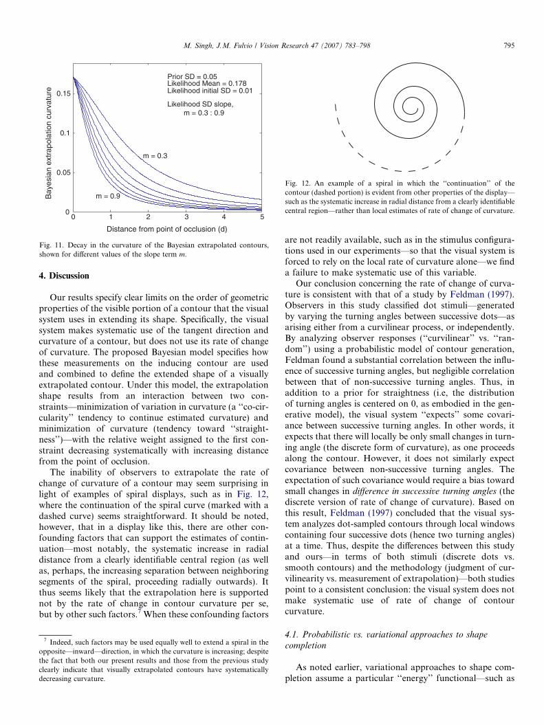
lik � wpr. As a result, jextð0Þ � llik ¼ ji, i.e., the extrapo-lation curvature near the point of occlusion essentiallyequals the estimated inducer curvature. With increasingdistance from the point of occlusion, the reliability of the‘likelihood’ constraint to continue inducer curvaturedecreases systematically (because of an increase in its vari-ance), whereas the variance of the prior remains constant.As a result, the curvature of the extrapolated contour isbiased more and more toward the ‘prior’ curvature ofzero—i.e., extrapolation curvature decreases asymptotical-ly to zero. The rate of curvature decay is modulated by theslope term m:

jextðdÞ ¼ ji �r2

pr

r2pr þ ðr0

lik þ mdÞ2ð10Þ

Fig. 11 plots this curvature decay for a number of differentvalues of m.

This probabilistic cue-combination model thus explainsthe decaying-curvature behavior of visually extrapolatedcontours. Importantly, although the model makes system-atic use of the curvature of the inducing contour, it involvesno dependence on its rate of change of curvature. As ourextrapolation experiments with Euler spirals show, thisproperty is consistent with human visual extrapolation.

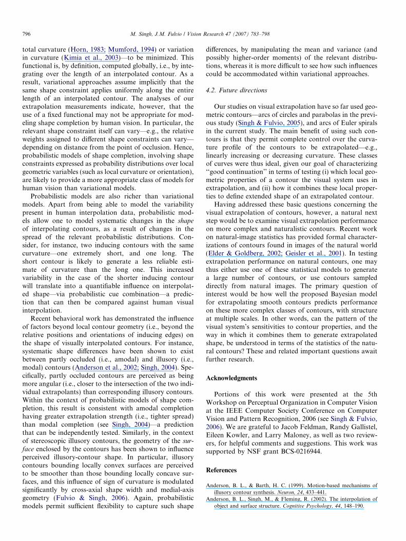
Fig. 12. An example of a spiral in which the ‘‘continuation’’ of thecontour (dashed portion) is evident from other properties of the display—such as the systematic increase in radial distance from a clearly identifiablecentral region—rather than local estimates of rate of change of curvature.

0 1 2 3 4 50

0.05

0.1

0.15

Prior SD = 0.05

Likelihood initial SD = 0.01Likelihood Mean = 0.178

Likelihood SD slope,m = 0.3 : 0.9

m = 0.3

m = 0.9

Distance from point of occlusion (d)

Bay

esia

n ex

trap

olat

ion

curv

atur

e

Fig. 11. Decay in the curvature of the Bayesian extrapolated contours,shown for different values of the slope term m.

M. Singh, J.M. Fulvio / Vision Research 47 (2007) 783–798 795

4. Discussion

Our results specify clear limits on the order of geometricproperties of the visible portion of a contour that the visualsystem uses in extending its shape. Specifically, the visualsystem makes systematic use of the tangent direction andcurvature of a contour, but does not use its rate of changeof curvature. The proposed Bayesian model specifies howthese measurements on the inducing contour are usedand combined to define the extended shape of a visuallyextrapolated contour. Under this model, the extrapolationshape results from an interaction between two con-straints—minimization of variation in curvature (a ‘‘co-cir-cularity’’ tendency to continue estimated curvature) andminimization of curvature (tendency toward ‘‘straight-ness’’)—with the relative weight assigned to the first con-straint decreasing systematically with increasing distancefrom the point of occlusion.

The inability of observers to extrapolate the rate ofchange of curvature of a contour may seem surprising inlight of examples of spiral displays, such as in Fig. 12,where the continuation of the spiral curve (marked with adashed curve) seems straightforward. It should be noted,however, that in a display like this, there are other con-founding factors that can support the estimates of contin-uation—most notably, the systematic increase in radialdistance from a clearly identifiable central region (as wellas, perhaps, the increasing separation between neighboringsegments of the spiral, proceeding radially outwards). Itthus seems likely that the extrapolation here is supportednot by the rate of change in contour curvature per se,but by other such factors.7 When these confounding factors

7 Indeed, such factors may be used equally well to extend a spiral in theopposite—inward—direction, in which the curvature is increasing; despitethe fact that both our present results and those from the previous studyclearly indicate that visually extrapolated contours have systematicallydecreasing curvature.

are not readily available, such as in the stimulus configura-tions used in our experiments—so that the visual system isforced to rely on the local rate of curvature alone—we finda failure to make systematic use of this variable.

Our conclusion concerning the rate of change of curva-ture is consistent with that of a study by Feldman (1997).Observers in this study classified dot stimuli—generatedby varying the turning angles between successive dots—asarising either from a curvilinear process, or independently.By analyzing observer responses (‘‘curvilinear’’ vs. ‘‘ran-dom’’) using a probabilistic model of contour generation,Feldman found a substantial correlation between the influ-ence of successive turning angles, but negligible correlationbetween that of non-successive turning angles. Thus, inaddition to a prior for straightness (i.e, the distributionof turning angles is centered on 0, as embodied in the gen-erative model), the visual system ‘‘expects’’ some covari-ance between successive turning angles. In other words, itexpects that there will locally be only small changes in turn-ing angle (the discrete form of curvature), as one proceedsalong the contour. However, it does not similarly expectcovariance between non-successive turning angles. Theexpectation of such covariance would require a bias towardsmall changes in difference in successive turning angles (thediscrete version of rate of change of curvature). Based onthis result, Feldman (1997) concluded that the visual sys-tem analyzes dot-sampled contours through local windowscontaining four successive dots (hence two turning angles)at a time. Thus, despite the differences between this studyand ours—in terms of both stimuli (discrete dots vs.smooth contours) and the methodology (judgment of cur-vilinearity vs. measurement of extrapolation)—both studiespoint to a consistent conclusion: the visual system does notmake systematic use of rate of change of contourcurvature.

4.1. Probabilistic vs. variational approaches to shape

completion

As noted earlier, variational approaches to shape com-pletion assume a particular ‘‘energy’’ functional—such as

796 M. Singh, J.M. Fulvio / Vision Research 47 (2007) 783–798

total curvature (Horn, 1983; Mumford, 1994) or variationin curvature (Kimia et al., 2003)—to be minimized. Thisfunctional is, by definition, computed globally, i.e., by inte-grating over the length of an interpolated contour. As aresult, variational approaches assume implicitly that thesame shape constraint applies uniformly along the entirelength of an interpolated contour. The analyses of ourextrapolation measurements indicate, however, that theuse of a fixed functional may not be appropriate for mod-eling shape completion by human vision. In particular, therelevant shape constraint itself can vary—e.g., the relativeweights assigned to different shape constraints can vary—depending on distance from the point of occlusion. Hence,probabilistic models of shape completion, involving shapeconstraints expressed as probability distributions over localgeometric variables (such as local curvature or orientation),are likely to provide a more appropriate class of models forhuman vision than variational models.

Probabilistic models are also richer than variationalmodels. Apart from being able to model the variabilitypresent in human interpolation data, probabilistic mod-els allow one to model systematic changes in the shapeof interpolating contours, as a result of changes in thespread of the relevant probabilistic distributions. Con-sider, for instance, two inducing contours with the samecurvature—one extremely short, and one long. Theshort contour is likely to generate a less reliable esti-mate of curvature than the long one. This increasedvariability in the case of the shorter inducing contourwill translate into a quantifiable influence on interpolat-ed shape—via probabilistic cue combination—a predic-tion that can then be compared against human visualinterpolation.

Recent behavioral work has demonstrated the influenceof factors beyond local contour geometry (i.e., beyond therelative positions and orientations of inducing edges) onthe shape of visually interpolated contours. For instance,systematic shape differences have been shown to existbetween partly occluded (i.e., amodal) and illusory (i.e.,modal) contours (Anderson et al., 2002; Singh, 2004). Spe-cifically, partly occluded contours are perceived as beingmore angular (i.e., closer to the intersection of the two indi-vidual extrapolants) than corresponding illusory contours.Within the context of probabilistic models of shape com-pletion, this result is consistent with amodal completionhaving greater extrapolation strength (i.e., tighter spread)than modal completion (see Singh, 2004)—a predictionthat can be independently tested. Similarly, in the contextof stereoscopic illusory contours, the geometry of the sur-

face enclosed by the contours has been shown to influenceperceived illusory-contour shape. In particular, illusorycontours bounding locally convex surfaces are perceivedto be smoother than those bounding locally concave sur-faces, and this influence of sign of curvature is modulatedsignificantly by cross-axial shape width and medial-axisgeometry (Fulvio & Singh, 2006). Again, probabilisticmodels permit sufficient flexibility to capture such shape

differences, by manipulating the mean and variance (andpossibly higher-order moments) of the relevant distribu-tions, whereas it is more difficult to see how such influencescould be accommodated within variational approaches.

4.2. Future directions

Our studies on visual extrapolation have so far used geo-metric contours—arcs of circles and parabolas in the previ-ous study (Singh & Fulvio, 2005), and arcs of Euler spiralsin the current study. The main benefit of using such con-tours is that they permit complete control over the curva-ture profile of the contours to be extrapolated—e.g.,linearly increasing or decreasing curvature. These classesof curves were thus ideal, given our goal of characterizing‘‘good continuation’’ in terms of testing (i) which local geo-metric properties of a contour the visual system uses inextrapolation, and (ii) how it combines these local proper-ties to define extended shape of an extrapolated contour.

Having addressed these basic questions concerning thevisual extrapolation of contours, however, a natural nextstep would be to examine visual extrapolation performanceon more complex and naturalistic contours. Recent workon natural-image statistics has provided formal character-izations of contours found in images of the natural world(Elder & Goldberg, 2002; Geisler et al., 2001). In testingextrapolation performance on natural contours, one maythus either use one of these statistical models to generatea large number of contours, or use contours sampleddirectly from natural images. The primary question ofinterest would be how well the proposed Bayesian modelfor extrapolating smooth contours predicts performanceon these more complex classes of contours, with structureat multiple scales. In other words, can the pattern of thevisual system’s sensitivities to contour properties, and theway in which it combines them to generate extrapolatedshape, be understood in terms of the statistics of the natu-ral contours? These and related important questions awaitfurther research.

Acknowledgments

Portions of this work were presented at the 5thWorkshop on Perceptual Organization in Computer Visionat the IEEE Computer Society Conference on ComputerVision and Pattern Recognition, 2006 (see Singh & Fulvio,2006). We are grateful to Jacob Feldman, Randy Gallistel,Eileen Kowler, and Larry Maloney, as well as two review-ers, for helpful comments and suggestions. This work wassupported by NSF grant BCS-0216944.

References

Anderson, B. L., & Barth, H. C. (1999). Motion-based mechanisms ofillusory contour synthesis. Neuron, 24, 433–441.

Anderson, B. L., Singh, M., & Fleming, R. (2002). The interpolation ofobject and surface structure. Cognitive Psychology, 44, 148–190.

M. Singh, J.M. Fulvio / Vision Research 47 (2007) 783–798 797

August, J., & Zucker, S. W. (2001). A Markov process using curvature forfiltering curve images. In M. A. T. Figueredo, J. Zeurbia, & A. K. Jain(Eds.), EMMCVPR 2001, energy minimization methods in computer

vision and pattern recognition (pp. 497–512). Sophia Antipolis, France:Springer-Verlag.

Barrow, H. G., & Tenenbaum, J. (1981). Interpreting line drawings asthree-dimensional surfaces. Artificial Intelligence, 17, 75–116.

Ben-Shahar, O., & Zucker, S. W. (2004). Geometrical computationsexplain projection patterns of long-range horizontal connections invisual cortex. Neural Computation, 16(3), 445–476.

Bosking, W., Zhang, Y. B. S., & Fitzpatrick, D. (1997). Orientationselectivity and the arrangement of horizontal connections in the treeshrew striate cortex. The Journal of Neuroscience, 17(6), 2112–2127.

Box, G. E. P., & Tiao, G. C. (1992). Bayesian inference in statistical

analysis. New York: Wiley.Brainard, D. H. (1997). The Psychophysics Toolbox. Spatial Vision, 10,

433–436.Bregman, A. L. (1981). Asking the ‘‘what for’’ question in auditory

perception. In M. L. Kubovy & J. R. Pomerantz (Eds.), Perceptual

organization (pp. 141–180). Hillsdale, NJ: Lawrence Erlbaum.Caelli, T. M., & Umansky, J. (1976). Interpolation in the visual system.

Vision Research, 16, 1055–1060.Clark, J. J., & Yuille, A. L. (1990). Data fusion for sensory information

processing systems. Boston, MA: Kluwer.Dobbins, A., Zucker, S. W., & Cynader, M. S. (1987). Endstopped

neurons in the visual cortex as a substrate for calculating curvature.Nature, 329(6138), 438–441.

Elder, J. H., & Goldberg, R. M. (2002). Ecological statistics of Gestaltlaws for the perceptual organization of contours. Journal of Vision,

2(4), 324–353.Euler, L. (1744/1952). De curvis elasticis. In C. Caratheodory (Ed.),

Methodus inventiendi lineas curvas maximi minimive proprietate

gaudentes sive solutio problematis isoperimetrici latissimo sensu

accepti. Opera Omnia, Ser. I.: Opera Mathematica (Vol. 24,pp. 308–342). Lausanne: Birkhauser [Originally published in 1744in book format].

Fantoni, C., & Gerbino, W. (2003). Contour interpolation by vector-fieldcombination. Journal of Vision, 3(4), 281–303.

Feldman, J. (1997). Curvilinearity, covariance, and regularity in percep-tual groups. Vision Research, 37(20), 2835–2848.

Feldman, J. (2001). Bayesian contour integration. Perception & Psycho-

physics, 63(7), 1171–1182.Feldman, J., & Singh, M. (2005). Information along contours and object

boundaries. Psychological Review, 112(1), 243–252.Field, D., Hayes, A., & Hess, R. (1993). Contour integration by the

human visual system: Evidence for a local ‘‘association field’’. Vision

Research, 33(2), 173–193.Fulvio, J., & Singh, M. (2006). Surface geometry influences the shape of

illusory contours. Acta Psychologica, 123, 20–40.Geisler, W. S., Perry, J. S., Super, B. J., & Gallogly, D. P. (2001). Edge co-

occurrence in natural images predicts contour grouping performance.Vision Research, 41(6), 711–724.

Grossberg, S., & Mingolla, E. (1985). Neural dynamics of form percep-tion: Boundary completion, illusory figures, and neon color spreading.Psychological Review, 92, 173–211.

Guttman, S. E., & Kellman, P. J. (2004). Contour interpolation revealedby a dot localization paradigm. Vision Research, 44, 1799–1815.

Heitger, F., von der Heydt, R., Peterhans, E., Rosenthaler, L., & Kubler,O. (1998). Simulation of neural contour mechanisms:representinganomalous contours. Image and Vision Computing, 16, 407–421.

Hon, A., Maloney, L., & Landy, M. (1997). The influence function forvisual interpolation. SPIE Conference Proceedings, 3016, 409–419.

Horn, B. K. P. (1983). The curve of least energy. ACM Transactions on

Mathematical Software, 9(4), 441–460.Kanizsa, G. (1979). Organization in vision: Essays on Gestalt perception.

New York: Prager.Kass, R. E., & Raftery, A. E. (1995). Bayes factors. Journal of the

American Statistical Association, 90(430), 773–795.

Kellman, P. J., & Shipley, T. F. (1991). A theory of visual interpolation inobject perception. Cognitive Psychology, 23, 141–221.

Kimia, B. B., Frankel, I., & Popescu, A. (2003). Euler spiral for shapecompletion. International Journal of Computer Vision, 54(1/2),157–180.

Klein, S. A., & Levi, D. M. (1987). Position sense of the peripheral retina.Journal of the Optical Society of America, A, 4, 1543–1553.

Kovacs, I., & Julesz, B. (1993). A closed curve is much more than anincomplete one: Effect of closure in figure-ground segmentation.Proceedings of the National Academy of Sciences, USA, 90,7495–7497.

Kubovy, M., & Gepshtein, S. (2000). Optimal curvatures in the comple-tion of visual contours. Investigative Ophthalmology and Visual

Science, 41(Suppl.), B568.Landy, M. S., Maloney, L. T., Johnston, E., & Young, M. (1995).

Measurement and modeling of depth cue combination: In defense ofweak fusion. Vision Research, 35(3), 389–412.

Link, N., & Zucker, S. W. (1988). Corner detection in curvilinear dotgrouping. Biological Cybernetics, 59, 247–256.

Love, A. E. H. (1927). Mathematical theory of elasticity. Cambridge:University Press.

Mardia, K. V., & Jupp, P. (2000). Directional statistics. New York: WileySeries in Probability and Statistics.

Mood, A., Graybill, F. A., & Boes, D. C. (1974). Introduction to the theory

of statistics (3rd ed.). New York: McGraw-Hill.Mumford, D. (1994). Elastica and computer vision. In C. L. Bajaj (Ed.),

Algebraic geometry and its applications (pp. 491–506). New York:Springer-Verlag.

Nakayama, K., He, Z., & Shimojo, S. (1995). Visual surface representa-tion: A critical link between lower-level and higher-level vision (2nded.. In S. M. Kosslyn & D. N. Osherson (Eds.). Visual cognition: An

invitation to cognitive science (Vol. 2, pp. 491–506). Cambridge, MA:MIT Press.

Parent, P., & Zucker, S. W. (1989). Trace inference, curvature consistencyand curve detection. IEEE Transactions on Pattern Analysis and

Machine Intelligence, 11, 823–839.Pelli, D. G. (1997). The Videotoolbox software for visual psycho-

physics: Transforming numbers into movies. Spatial Vision, 10,437–442.

Pettet, M. W., McKee, S. P., & Grzywacz, N. M. (1998). Constraints onlong range interactions mediating contour detection. Vision Research,

38(6), 865–879.Pizlo, Z., Salach-Goyska, M., & Rosenfeld, A. (1997). Curve detection in a

noisy image. Vision Research, 37(9), 1217–1241.Ringach, D. L., & Shapley, R. (1996). Spatial and temporal properties of

illusory contours and amodal boundary completion. Vision Research,

36(20), 3037–3050.Schwarz, G. (1978). Estimating the dimension of a model. The Annals of

Statistics, 6, 461–464.Sigman, M., Cecchi, G. A., Gilbert, C. D., & Magnasco, M. O. (2001). On

a common circle: Natural scenes and Gestalt rules. Proceedings of the

National Academy of Sciences, USA, 98(4), 1935–1949.Singh, M. (2004). Modal and amodal completion generate different

shapes. Psychological Science, 15, 454–459.Singh, M., & Fulvio, J. M. (2005). Visual extrapolation of contour

geometry. Proceedings of the National Academy of Sciences, USA,

102(3), 939–944.Singh, M., & Fulvio, J. (2006). Contour extrapolation using probabilistic

cue combination. In Proceedings of the conference on computer visionand pattern recognition (Workshop on perceptual organization incomputer vision). http://dx.doi.org/10.1109/CVPRW.2006.61.

Singh, M., & Hoffman, D. D. (1999). Completing visual contours: Therelationship between relatability and minimizing inflections. Perception

& Psychophysics, 61, 636–660.Smits, J. T., & Vos, P. G. (1987). The perception of continuous curves in

dot stimuli. Perception, 16, 121–131.Takeichi, H. (1995). The effect of curvature on visual interpolation.

Perception, 24, 1011–1020.

798 M. Singh, J.M. Fulvio / Vision Research 47 (2007) 783–798

Takeichi, H., Nakazawa, H., Murakami, I., & Shimojo, S. (1995). Thetheory of the curvature-constraint line for amodal completion.Perception, 24, 373–389.

Ullman, S. (1976). Filling-in the gaps: The shape of subjective contoursand a model for their generation. Biological Cybernetics, 25, 1–6.

Uttal, W. R. (1973). The effect of deviations from linearity on thedetection of dotted line patterns. Vision Research, 13, 2155–2163.

Warren, P. A., Maloney, L. T., & Landy, M. S. (2002). Interpolatingsampled contours in 3D: Analyses of variability and bias. Vision

Research, 42(21), 2431–2446.Warren, P. A., Maloney, L. T., & Landy, M. S. (2004). Interpolating

sampled contours in 3D: Perturbation analyses. Vision Research, 44(8),815–832.

Wichmann, F. A., & Hill, N. J. (2001). The psychometric function: I.Fitting, sampling and goodness-of-fit. Perception & Psychophysics,

63(8), 1293–1313.Yuille, A. L., Fang, F., Schrater, P., & Kersten, D. (2004). Human

and ideal observers for detecting image curves. In S. Thrun, L.Saul, & B. Scholkopf (Eds.). Advances in neural information

processing systems (Vol. 16, pp. 59–70). Cambridge, MA: MITPress.

Zucker, S. W., & Davis, S. (1988). Points and endpoints: A size/spacingconstraint in dot grouping. Perception, 17, 229–247.

Zucker, S. W., Dobbins, A., & Iverson, L. (1989). Two stages of curvedetection suggest two styles of visual computation. Neural Computa-

tion, 1, 68–81.