Bio medical Imaging

? Pergamon

Computerized Medical Imagmg and Graphics. Vol. 19, No. I. pp. 3-25, 1995 Copyright 0 1995 Elsevier Science Ltd Printed in the USA. All rights reserved

0895.61 I l/95 $9.50 + .oO

0895-6111(94)00043-3

BIOMEDICAL IMAGING MODALITIES: A TUTORIAL

Raj Acharya,’ Richard Wasserman, Jeffrey Stevens, and Carlos Hinojosa Department of Electrical and Computer Engineering, Biomedical Imaging Group (BMIG), 201 Bell Hall,

State University of New York at Buffalo, Buffalo, NY 14260, USA, E-mail: [email protected]

(Received 9 May 1994)

Abstract-The introduction of advanced imaging technologies has improved significantly the quality of medical care available to patients. Non-invasive imaging modalities allow a physician to make increasingly accurate diagnoses and render precise and measured modes of treatment. Current uses of imaging technologies include laboratory medicine, surgery, radiation therapy, nuclear medicine, and diagnostic radiology. This paper provides an overview of most of the popular imaging modalities currently in clinical use. It is hoped that a general understanding of the modality from which an image is derived will help researchers in the subsequent analysis of the image data.

Key Weds: Tutorial, PET, MRI, CT, Medical imaging, DSA, Ultrasound, Squid

1 INTRODUCTION

The Introduction of advanced imaging technologies has improved significantly the quality of medical care available to patients. Noninvasive imaging modalities allow a physician to make increasingly accurate diagnoses and render precise and measured modes of treatment. Current uses of imaging technologies include laboratory medicine, surgery, radiation therapy, nuclear medicine, and diagnostic radiology. Common medical imaging methodologies may be divided grossly into two general groupings: (a) techniques that seek to image internal anatomical structures and (b) methods that present mappings of physiological function.

Rapid technological advances have made the acquisition of three and four-dimensional (4D) represen- tations of human and animal internal structures com- monplace. A multitude of imaging modalities are available currently.

X-Ray Computed Tomography (CT) is a popular modality which is used routinely in clinical practice. CT generates a three-dimensional (3D) image set that is representative of a patient’s anatomy. CT scanners produce a set of two-dimensional (2D), axial cross section images which may be stacked to form a 3D data :set. The mathematics of CT image reconstruction is also employed in many additional imaging modalities. The problem associated with CT reconstruction was solved by Radon in 19 17. The availability of high

’ To whom correspondence should be addressed.

3

speed computers and relatively inexpensive memories allow modem scanners to utilize sophisticated reconstruction algorithms. The majority of current X-Ray CT scanners collect 3D images, at the rate of one 2D slice at a time. Specialized scanners are also available which collect an entire 3D volume within a very short time span.

Magnetic Resonance Imaging (MRI) is similar to CT imaging in that it generates 3D data sets corresponding to a patient’s anatomy. However, MRI differs funda- mentally from CT in the manner in which images are acquired. CT scanners employ x-ray radiation to generate the data needed to reconstruct internal structures. Alternatively, MRI utilizes RF waves and magnetic fields to obtain 3D images and is based on the principle of Nuclear Magnetic Resonance (NMR). MRI scanners utilize non-ionizing beams and provide unparalleled soft tissue contrast in a noninvasive manner.

Emission CT techniques obtain 3D representa-

tions of the location of injected pharmaceuticals. The injected pharmaceuticals are labelled with gamma ray emitting radionuclides. The emitted gamma rays are measured at sites external to a patient. Such measured data may be utilized to reconstruct a 3D mapping of internal emission density. A 3D image is generated by reconstructing a measured set of 2D projection images acquired at various angles around the patient. Emission Tomography differs from MRI and CT in that it provides physiological function information, such as per- fusion and metabolism, as opposed to strictly anatomical information.

Another methodology which gathers functional

4 Computerized Medical Imaging and Graphics January-Februaryll995, Volume 19, Number 1

information is Biomagnetic Source Imaging. This tech-

nology allows for the external measurement of the low level magnetic fields generated by neuron activity. Bio- magnetic source imaging allows a clinician to gather data concerning brain function that has previously proved elusive (I).

Ultrasound based imaging techniques comprise a set of methodologies capable of acquiring both quantitative and qualitative diagnostic information. Many ultrasound based methods are attractive due to their ability to obtain real time imagery, employing compact and mobile equipment, at a significantly lower cost than is incurred with other medical imaging modalities. The real time nature of ultrasound makes it possible for physicians to observe the motion of structures inside a patient’s body. This ability has resulted in the wide- spread use of ultrasound technology in the fields of pediatrics and cardiology. Equipment which employs doppler echo techniques can extract quantitative velocity information such as the rate of blood flow in a vessel of interest. Additionally, the introduction of ultrasound signals into a patient, at the levels currently employed, has been determined to be safe (2). The lack of negative effects from exposure, portability of equipment, relatively low cost and quantitative acquisition modes distinguishes ultrasound techniques as an important class of medical imaging technology.

This paper provides an overview of most of the popular imaging modalities currently in clinical use. The foregoing discussion limits the use of advanced mathematical concepts, instead employing intuitive de- scriptions of each medical modality. It is hoped that a general understanding of the modality from which an image is derived will help researchers in the subsequent analysis of the image data.

The sections to follow include discussions of X- Ray CT (section 2), MRI (section 3), Emission CT (section 4) Biomagnetic source imaging (section 5), Digital Subtraction Angiography (section 6), and ultrasound imaging techniques (section 7).

2 X-RAY COMPUTED TOMOGRAPHY

X-ray CT or Computed Axial Tomography (CAT) is a medical imaging modality which is capable of noninvasively acquiring a 3D representation of a patient’s internal anatomical structure. This 3D representation may be visualized from an arbitrary viewpoint, providing vital information for anatomical mapping, tumor localization, stereotactic surgery planning and many other diagnostic applications (3).

Physicians have long utilized x-ray based imaging systems for non-invasive medical diagnostics. In the

case of the conventional radiograph, a patient is placed in front of an x-ray source which transmits radiation through the subject’s body. Each x-ray incident on the patient is attenuated by the tissues it passes through along its linear flight path. Differing tissue types in the body exhibit differing densities with respect to x-ray radiation. Each tissue type may therefore be assigned a value ,LL(X, y, Z) which denotes the tissue density at Cartesian coordinate (x, y, z). The line integral of these tissue densities,

s= s pL(x, y, z)dl. (1)

is proportional to the attenuation experienced by an x- ray passing along the given path. A 2D projection image or “shadow” of these x-rays is imaged by measur- ing the x-ray energy leaving the patient’s body in some 2D region of interest. Conventional radiography is a limited diagnostic modality, in the sense that it produces a 2D projection of a 3D object. Consequently, a large amount of information concerning internal anatomical structure is unavailable to the radiologist.

X-ray CT is a modality that is built upon the same physical principles that form the basis of conventional radiography. Differing tissue types possess different linear attenuation coefficients. This fact is utilized in conjunction with x-ray shadows from multiple viewpoints in order to reconstruct a representation of internal anatomical structure.

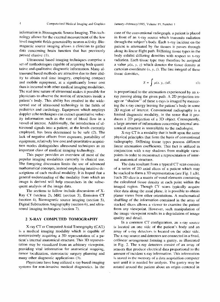
The data resultant from a typical CT scan consists of a series of 2D axial slices of a patient which may be stacked to form a 3D representation (see Fig. 1 a,b). Each 2D slice is a matrix of voxel elements containing the calculated tissue density at each point within the imaged region. Though CT scans typically acquire slice data along the axial plane, it is possible to obtain planar views from other orientations. A mathematical shuffling of the information contained in the array of stacked slices allows a viewer to examine the patient from any viewpoint. However, such manipulation of the image viewpoint results in a degradation of image quality and detail.

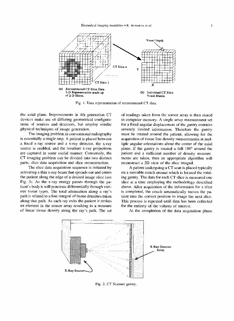
In a common CT configuration, an x-ray source is located on one side of the patient’s body and an array of x-ray detectors is located on the other side. The x-ray source and detectors are connected in a fixed, collinear arrangement forming a gantry, as illustrated in Fig. 2. The x-ray detectors consist of an array of sensors that produce electrical data proportional to the amount of incident x-ray information. This information is stored in the memory of a data acquisition computer unit until it is needed for analysis. The gantry may be rotated around the patient about an origin centered in

Biomedical imaging modalities l R. ACHARYA et al.

CT Slice n Y

X

(a) Reconstructed CT Slice Data 3-D Representation made up (b) Individual CT Slice of 2-D Slices. Voxel Matrix

Fig. 1. Data representation of reconstructed CT data.

the axial plane. Improvements in 4th generation CT devices make use of differing geometrical configurations of sources and detectors, but employ similar physical techniques of image generation.

The imaging problem in conventional radiography is essentially a single step. A patient is placed between a fixed x-ray source and a x-ray detector, the x-ray source is enabled, and the resultant x-ray projections are captured in some useful manner. Conversely, the CT imaging problem can be divided into two distinct parts, slice data acquisition and slice reconstruction.

The slice data acquisition sequence is initiated by activating a thin x-ray beam that spreads out and enters the patient along the edge of a desired image slice (see Fig. 3). As the x-ray energy passes through the patient’s body it will penetrate differentially through various tissue types. The total attenuation along a ray’s path is related to a line integral of tissue densities taken along that path. As each ray exits the patient it strikes an element in the sensor array resulting in a measure of linear tissue density along the ray’s path. The set

X-Ray Soured

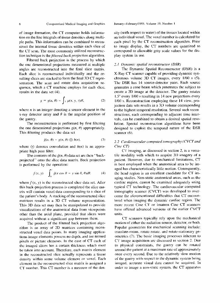
of readings taken from the sensor array is then stored in computer memory. A single array measurement set for a fixed angular displacement of the gantry contains severely limited information. Therefore the gantry must be rotated around the patient, allowing for the acquisition of tissue line density measurements at multiple angular orientations about the center of the axial plane. If the gantry is rotated a full 180” around the patient and a sufficient number of density measurements are taken, then an appropriate algorithm will reconstruct a 2D view of the slice imaged.

A patient undergoing a CT scan is placed typically on a movable couch around which is located the rotating gantry. The data for each CT slice is measured one slice at a time employing the methodology described above. After acquisition of the information for a slice is completed, the couch automatically moves the patient into the correct position to image the next slice. This process is repeated until data has been collected for the entirety of the volume of interest.

At the completion of the data acquisition phase

X-Ray Detector Anay

Fig. 2. CT Scanner gentry.

6 Computerized Medical Imaging and Graphics January-February/l995 Volume 19, Number I

of image formation, the CT computer holds informa- sity (with respect to water) of the tissues located within tion on the line integrals of tissue densities along multi- an individual voxel. The voxel number is calculated for ple paths. This information can be combined to recon- each pixel by the CT reconstruction algorithm. Prior struct the internal tissue densities within each slice of to image display, the CT numbers are quantized to the CT scan. The most commonly utilized reconstruc- correspond to allowable gray scale values for the dis- tion technique is thejiltered buck projection algorithm. play system in use.

Filtered back projection is the process by which the one dimensional projections measured at multiple angles are reconstructed into the final slice matrix. Each slice is reconstructed individually and the resulting slices are stacked to form the final 3D CT representation. The scan and rotate data acquisition sequence, which a CT machine employs for each slice, results in the data set (4).

2. I Dynumic spatial reconstructor (DSR) The Dynamic Spatial Reconstructor (DSR) is a

X-Ray CT scanner capable of providing dynamic syn- chronous volume 3D CT images, every l/60 s (5). The DSR has 14 source-detector pairs. Each source generates a cone beam which penetrates the subject to create a 2D image at the detector. The gantry rotates 1 S” every l/60 s resulting in 14 new projections every l/60 s. Reconstruction employing these 14 view, projection data sets results in a 3D volume corresponding to the highest temporal resolution. Several such recon- structions, each corresponding to adjacent time intervals, can be combined to obtain a desired spatial resolution. Special reconstruction algorithms have been designed to exploit the temporal nature of the DSR scanner (6).

where n is an integer denoting a sensor element in the x-ray detector array and 19 is the angular position of the gantry.

The reconstruction is performed by first filtering the one dimensional projections g(n, 0) appropriately. This filtering produces the data set

2(fl> f)) = R(n, H) 0 h(n), (3)

where @ denotes convolution and h(n) is an appropriate high pass filter.

The contents of the&n, 8) data set are then “back- projected” onto the slice data matrix. Back projection is performed by the operation:

f(x. y) = s

* ^ ~(x cos 0 + y sin 8, 19)dB. (4) 0

wheref(x, y) is the reconstructed slice data set. After this back-projection process is completed the slice matrix will contain voxel data corresponding to a slice of the patient’s body. A stacking of the reconstructed slice matrices results in a 3D CT volume representation. This 3D data set may then be manipulated to provide visualizations of the anatomical data from viewpoints other than the axial plane, provided that slices were acquired without a significant gap between them.

The product of the filtered back projection algorithm is an array of 2D matrices containing reconstructed voxel data points. In many imaging applications image elements possess no depth, and are termed pixels or picture elements. In the case of CT each of the imaged slices has a certain thickness which must be taken into account. Therefore, each matrix element in the reconstructed slice actually represents a tissue density within some volume element or voxel. Each element in the reconstructed slice matrix is assigned a CT number. This CT number is a measure of the den-

2.2 Cardiovascular computed tomogruphy (CVCT and Cine CT)

CT imaging, as discussed in section 2, is a versa- tile modality with which to acquire 3D imagery of a patient. However, due to mechanical limitations, CT is best employed when the anatomical area to be imaged has characteristically little motion. Consequently, the head region is an excellent candidate for CT imaging studies. Non-static anatomical areas, such as the cardiac region, cannot be examined adequately using typical CT technology. The cardiovascular computed tomography scanner (CVCT) was developed to over- come the aforementioned difficulties that CT encountered when imaging the dynamic cardiac region. The more recent Cine CT or lmatron Cine CT scanners have offered advanced versions of the earlier CVCT units.

CT scanners typically rely upon the mechanical motion of either the radiation source, detector, or both. Popular geometries for mechanical scanning include: translate-rotate, rotate-rotate, and rotate-stationary geometries (7). The basic imaging processes inherent to CT image acquisition are discussed in section 2. Due to physical constraints, the gantry can be rotated around the patient at a maximum rate of approximately once every second. Due to the relatively slow motion of the gantry with respect to the dynamic system being imaged, accurate visual data cannot be acquired. In order to image a non-static system, the CT apparatus

Biomedical imaging modalities l R. ACHAKYA et

CT Scan Employing A Rotating

Gantry and Adjustable Couch

Fig. 3. CT Scanner methodology

must be able to acquire imagery significantly faster than the system’s rate of change. If image acquisition is rapid enough, a single reconstructed image can be viewed as having occurred at a single instant of time. Consequently, a series of such high speed images would present a visual record of a system’s motion. Due I:O the data acquisition techniques employed in CT, rapid image formation requires that the gantry rotate at high speeds. In the case of cardiac imagery, the acquisition time required, for each complete image is of l.he order of milliseconds. Due to the mechanical nature of the CT gantry such rotation speeds are not feasible.

The rate of CT image acquisition can be increased significantly by replacing the mechanical gantry system with an electrostatic scanning apparatus. As al- luded to previously, the angular sampling rate (4) must be increased in order to achieve clinically useful motion imagery of the heart. Electrostatic scanning techniques are capable of generating angular sampling rates at least an order of magnitude higher than those possible via mechanical systems. The common television employs a form of electronic scanning. An electron beam is scanned over the television surface in order to produce the desired picture. The beam is rapidly swepl across the entire viewing area of the screen. As long as the beam is swept at a high enough rate, each pixel on the television’s monitor appears to be illumi- nated simultaneously. Such a common example illustrates the high speed capabilities of electrostatic scanning methods.

The cardiovascular computed tomography scan-

ner (CVCT), developed between 1978 and 1982 utilizes electronic scanning. It is capable of providing multiple 1 cm. slices through the heart at scan rates of 50 ms. The scanner consists of an electron beam source, deflection coils, stationary target rings, detector rings, and a data acquisition system (7). Electron beams are generated at the head of the scanner. These beams pass through deflection coils which direct them towards one of four target rings. The target rings are located below the patient under the region of interest.

Each target ring corresponds to two adjacent slices in the subject. The target rings redirect the incident electron beams upward through the patient. This radiation passes through the patient as in the case of CT. The radiation exiting the body is collected by detector rings on the anterior side of the patient. The angular projection information collected can be varied electronically in such a system. Deflection coil characteristics may be altered electronically. Such changes in the coils’ characteristics modify the angle at which projection data is obtained. This angular measurement position may be varied rapidly, resulting in the collection of data at a significantly higher rate than is possible in mechanical systems. CVCT scanners employ the discussed methodology to capture cardiac imagery at a high enough rate to allow for motion analysis of a heart under study.

3 MAGNETIC RESONANCE IMAGING

Magnetic resonance imaging represents a major innovation in medical imaging technology. MR im-

8 Computerized Medical Imaging and Graphics January-February/l995, Volume 19, Number 1

e- .............................................................................................. ............................................................................................................................................................................................ ................................................................. ..s ................................................................................................ < .....................

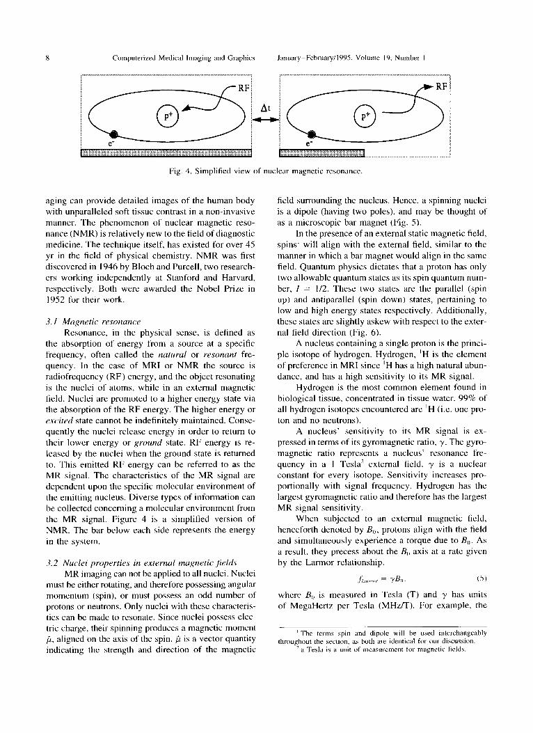
Fig. 4. Simplified view of nuclear magnetic resonance

aging can provide detailed images of the human body with unparalleled soft tissue contrast in a non-invasive manner. The phenomenon of nuclear magnetic resonance (NMR) is relatively new to the field of diagnostic medicine. The technique itself, has existed for over 45 yr in the field of physical chemistry. NMR was first discovered in 1946 by Bloch and Purcell, two researchers working independently at Stanford and Harvard, respectively. Both were awarded the Nobel Prize in 1952 for their work.

3. I Mupetic resonance Resonance, in the physical sense, is defined as

the absorption of energy from a source at a specific frequency, often called the natural or resonant frequency. In the case of MRI or NMR the source is radiofrequency (RF) energy, and the object resonating is the nuclei of atoms, while in an external magnetic field. Nuclei are promoted to a higher energy state via the absorption of the RF energy. The higher energy or excited state cannot be indefinitely maintained. Conse- quently the nuclei release energy in order to return to their lower energy or ground state. RF energy is released by the nuclei when the ground state is returned to. This emitted RF energy can be referred to as the MR signal. The characteristics of the MR signal are dependent upon the specific molecular environment of the emitting nucleus. Diverse types of information can be collected concerning a molecular environment from the MR signal. Figure 4 is a simplified version of NMR. The bar below each side represents the energy in the system.

3.2 Nuclei properties in external magnetic jields MR imaging can not be applied to all nuclei. Nuclei

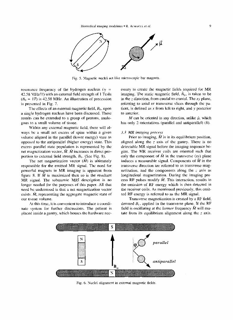
must be either rotating, and therefore possessing angular momentum (spin), or must possess an odd number of protons or neutrons. Only nuclei with these characteristics can be made to resonate. Since nuclei possess electric charge, their spinning produces a magnetic moment ,G, aligned on the axis of the spin. fi is a vector quantity indicating the strength and direction of the magnetic

field surrounding the nucleus. Hence, a spinning nuclei is a dipole (having two poles), and may be thought of as a microscopic bar magnet (Fig. 5).

In the presence of an external static magnetic field, spins’ will align with the external field, similar to the manner in which a bar magnet would align in the same field. Quantum physics dictates that a proton has only two allowable quantum states as its spin quantum number, I = l/2. These two states are the parallel (spin up) and antiparallel (spin down) states, pertaining to low and high energy states respectively. Additionally, these states are slightly askew with respect to the external field direction (Fig. 6).

A nucleus containing a single proton is the principle isotope of hydrogen. Hydrogen, ‘H is the element of preference in MRI since ‘H has a high natural abundance, and has a high sensitivity to its MR signal.

Hydrogen is the most common element found in biological tissue, concentrated in tissue water. 99% of all hydrogen isotopes encountered are ‘H (i.e. one proton and no neutrons).

A nucleus’ sensitivity to its MR signal is ex- pressed in terms of its gyromagnetic ratio, y. The gyromagnetic ratio represents a nucleus’ resonance frequency in a 1 Tesla’ external field. y is a nuclear constant for every isotope. Sensitivity increases pro- portionally with signal frequency. Hydrogen has the largest gyromagnetic ratio and therefore has the largest MR signal sensitivity.

When subjected to an external magnetic field, henceforth denoted by &, protons align with the field and simultaneously experience a torque due to B,,. As a result, they precess about the & axis at a rate given by the Larmor relationship.

,f;l,r,,,,>, = Y&j. (5)

where B(, is measured in Tesla (T) and y has units of MegaHertz per Tesla (MHz/T). For example, the

’ The terms spin and dipole will be used interchangeably throughout the section, as both are identical for our discussion.

’ a Tesla is a unit of measurement for magnetic t&Ids.


Fig. 5. Magnetic nuclei act like microscopic bar magnets.

resonance frequency of the hydrogen nucleus (y = 42.58 MHz/T) with an external field strength of I Tesla (B, = 17’) is 42.58 MHz. An illustration of precession is presented in Fig. 7.

The effects of an external magnetic field, BO, upon a single hydrogen nucleus have been discussed. These results can be extended to a group of protons, analo- gous to a small volume of tissue.

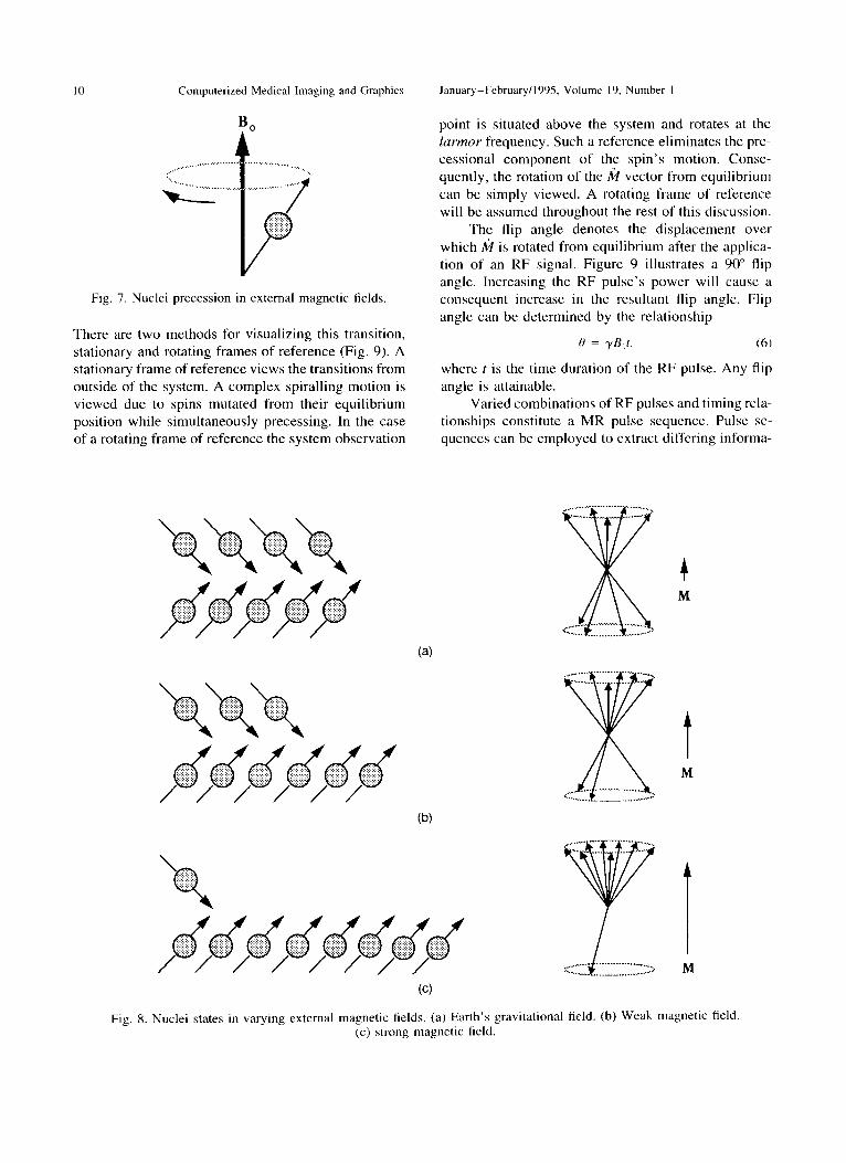
Within any external magnetic field, there will al- ways be a small net excess of spins within a given volume aligned in the parallel (lower energy) state as opposed to the antiparallel (higher energy) state. This excess parallel state population is represented by the net magnetization vector, &l. k increases in direct pro- portion to external tield strength, B,). {See Fig. 8).

The net magnetization vector (M) is ultimately responsible for the emitted MR signal. The need for powerful magnets in MR imaging is apparent from figure 8. If k is maximized then so is the resultant MR signal. The subatomic MRI description is no longer needed for the purposes of this paper. All that need be understood is that a net magnetization vector exists. k, representing the aggregate magnetic state of our tissue volume.

At this time, it is convenient to introduce a coordinate system for further discussions. The patient is placed inside a gantry, which houses the hardware nec-

essary to create the magnetic fields required for MR imaging. The static magnetic field, &,, is taken to be in the z direction, from caudal to cranial. The xy plane, referring to axial or transverse slices through the patient, is defined as x from left to right, and y posterior

to anterior. M can be oriented in any direction, unlike ,G, which

has only 2 orientations (parallel and antiparallel) (8).

3.3 MR imaging process

Prior to imaging, fi is in its equilibrium position, aligned along the z axis of the gantry. There is no detectable MR signal before the imaging sequence begins. The MR receiver coils are oriented such that only the component of fi in the transverse (xy) plane induces a measurable signal. Components of & in the transverse direction are referred to as transverse magnetization, and the components along the z axis as longitudinal magnetization. During the imaging process RF pulses modify k. This interaction, results in the emission of RF energy which is then detected in the receiver coils. As mentioned previously, this emitted RF energy is referred to as the MR signal.

Transverse magnetization is created by a RF field, denoted B,, applied in the transverse plane. If the RF field is oscillating at the lurmor frequency k will mu- tate from its equilibrium alignment along the z axis.

Fig. 6. Nuclei alignment in external magnetic fields.

I 0 Computerized Medical Imaging and Graphics January_February/l995, Volume 19, Number I

Bo

,... .. t

~,~,_,.,._..~~ ........ ........ . . . .._. ,., &. ._.

‘I

., .__....... i’ .:::. : ::: i:,: :: :.:.: : :.: :.. . . : lp Fig. 7. Nuclei precession in external magnetic fields.

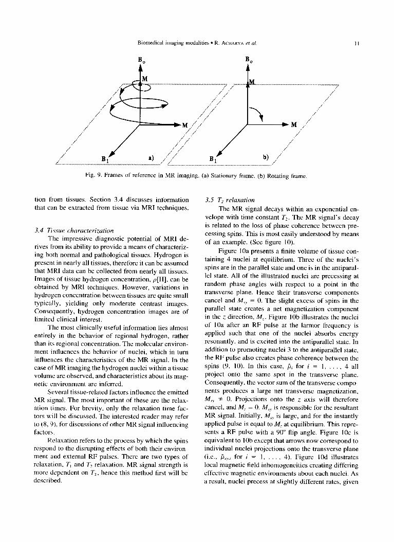
There are two methods for visualizing this transition, stationary and rotating frames of reference (Fig. 9). A stationary frame of reference views the transitions from outside of the system. A complex spiralling motion is viewed due to spins mutated from their equilibrium position while simultaneously precessing. In the case of a rotating frame of reference the system observation

point is situated above the system and rotates at the larmor frequency. Such a reference eliminates the pre- cessional component of the spin’s motion. Conse- quently, the rotation of the k vector from equilibrium can be simply viewed. A rotating frame of reference will be assumed throughout the rest of this discussion.

The flip angle denotes the displacement over which k is rotated from equilibrium after the application of an RF signal. Figure 9 illustrates a 90” flip angle. Increasing the RF pulse’s power will cause a consequent increase in the resultant flip angle. Flip angle can be determined by the relationship

0 = yB,r. (6)

where t is the time duration of the RF pulse. Any flip

angle is attainable. Varied combinations of RF pulses and timing rela-

tionships constitute a MR pulse sequence. Pulse sequences can be employed to extract differing informa-

_.I.----- ...‘3.r >

- .... x .

c. ..--. ._._

.. ......... ...-<. (4

,CC,_ ............ ._., -.-+. ......... . x 2-

-.. 2

... ..l _. .... I.-

(b) *_...- .- ._~. . . . . ..- 7 <- _. .- . . . . . . _ -. -._ . . . . __ . . . . . . . -.-.’

+

M

t

M

1

M

Fig. 8. Nuclei states in varying external magnetic fields. (a) Earth’s gravitational field. (b) Weak magnetic field (c) strong magnetic field.

Biomedical imaging modalities l R. ACHARYA et al. II

Fig. 9. Frames of reference in MR imaging. (a) Stationary frame. (b) Rotating frame.

tion from tissues. Section 3.4 discusses information that can be extracted from tissue via MRI techniques.

3.4 7issue characterization

The impressive diagnostic potential of MRI de- rives from its ability to provide a means of characteriz- ing both normal and pathological tissues. Hydrogen is present in nearly all tissues, therefore it can be assumed that MRI data can be collected from nearly all tissues. Images of tissue hydrogen concentration, p[H], can be obtained by MRI techniques. However, variations in hydrogen concentration between tissues are quite small typically, yielding only moderate contrast images. Consequently, hydrogen concentration images are of limited clinical interest.

The most clinically useful information lies almost entirely in the behavior of regional hydrogen, rather than its regional concentration. The molecular environment influences the behavior of nuclei, which in turn influences the characteristics of the MR signal. In the case of MR imaging the hydrogen nuclei within a tissue volume are observed, and characteristics about its magnetic environment are inferred.

Several tissue-related factors influence the emitted MR signal. The most important of these are the relaxation times. For brevity, only the relaxation time factors will be discussed. The interested reader may refer to (8, 9), for discussions of other MR signal influencing factors.

Relaxation refers to the process by which the spins respond to the disrupting effects of both their environment and external RF pulses. There are two types of relaxation, T, and T2 relaxation. MR signal strength is more dependent on T2, hence this method first will be described.

3.5 T2 relaxation

The MR signal decays within an exponential envelope with time constant T2. The MR signal’s decay

is related to the loss of phase coherence between precessing spins. This is most easily understood by means

of an example. (See figure 10).

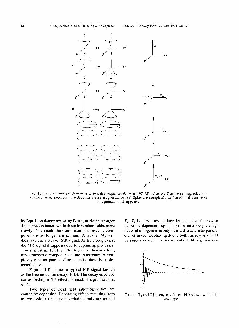
Figure 10a presents a finite volume of tissue containing 4 nuclei at equilibrium. Three of the nuclei’s spins are in the parallel state and one is in the antiparallel state. All of the illustrated nuclei are precessing at

random phase angles with respect to a point in the transverse plane. Hence their transverse components cancel and M,, = 0. The slight excess of spins in the parallel state creates a net magnetization component in the z, direction, M,. Figure lob illustrates the nuclei of IOa after an RF pulse at the larmor frequency is applied such that one of the nuclei absorbs energy resonantly, and is excited into the antiparallel state. In addition to promoting nuclei 3 to the antiparallel state, the RF pulse also creates phase coherence between the

spins (9, 10). In this case, pi for i = 1, . . , 4 all project onto the same spot in the transverse plane. Consequently, the vector sum of the transverse compo-

nents produces a large net transverse magnetization, M,, f 0. Projections onto the z axis will therefore cancel, and A4? = 0. M,, is responsible for the resultant MR signal. Initially, M,, is large, and for the instantly

applied pulse is equal to MZ at equilibrium. This represents a RF pulse with a 90” flip angle. Figure 1Oc is

equivalent to 1 Ob except that arrows now correspond to individual nuclei projections onto the transverse plane (i.e., fi.r ,,,, for i = 1, . . , 4). Figure 1Od illustrates local magnetic field inhomogeneities creating differing effective magnetic environments about each nuclei. As a result, nuclei precess at slightly different rates, given

12 Computerized Medical Imaging and Graphics January_February/l995. Volume 19. Number I

Fig. IO. Tz relaxation: (a) System prior to pulse sequence. (b) After 90” RF pulse. (c) Transverse magnetization. (d) Dephasing proceeds to reduce transverse magnetization. (e) Spins are completely dephased, and transverse

magnetization disappears.

by Eqn 4. As demonstrated by Eqn 4, nuclei in stronger fields precess faster, while those in weaker fields, more slowly. As a result, the vector sum of transverse components is no longer a maximum. A smaller IV,,, will then result in a weaker MR signal. As time progresses,

the MR signal disappears due to dephasing processes. This is illustrated in Fig. IOe. After a sufficiently long time, transverse components of the spins return to completely random phases. Consequently, there is no detected signal.

Figure I 1 illustrates a typical MR signal known as the free induction decay (FID). The decay envelope corresponding to Tf effects is much sharper than that of T,.

Two types of local field inhomogeneities are caused by dephasing. Dephasing effects resulting from microscopic intrinsic field variations only are termed

T2. T, is a measure of how long it takes for M,,, to decrease, dependent upon intrinsic microscopic magnetic inhomogeneities only. It is a characteristic param- eter of tissue. Dephasing due to both microscopic field variations as well as external static field (B,) inhomo-

Fig. II. T2 and TT decay envelopes, FID shown within Tf envelope.

Biomedical imaging modalities l R. ACHARYA et d. 13

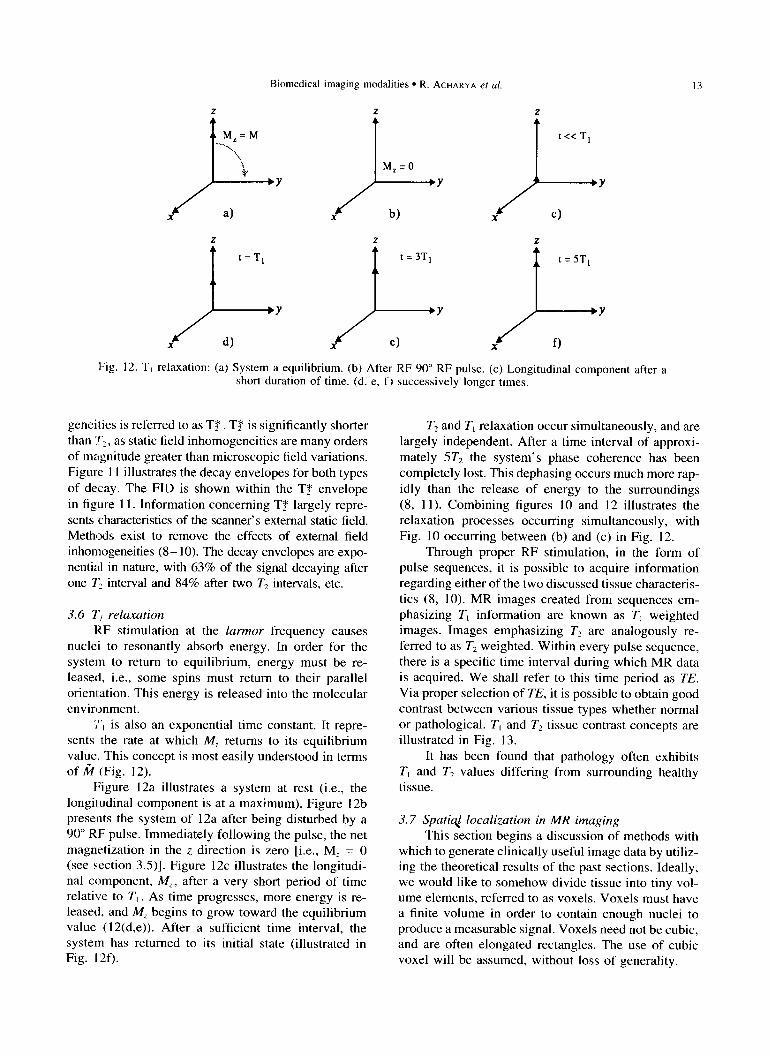
Fig. 12. T, relaxation: (a) System a equilibrium. (b) After RF 90” RF pulse. (c) Longitudinal component after a short duration of time. (d, e, f) successively longer times.

geneities is referred to as T$ T$ is significantly shorter than :f,, as static field inhomogeneities are many orders of magnitude greater than microscopic field variations. Figure 11 illustrates the decay envelopes for both types

of decay. The FID is shown within the T$ envelope in figure 1 1. Information concerning T$# largely represents characteristics of the scanner’s external static field. Methods exist to remove the effects of external field inhomogeneities (8- 10). The decay envelopes are exponential in nature, with 63% of the signal decaying after one l’Z interval and 84% after two T2 intervals, etc.

3.6 T, relaxation KF stimulation at the larmor frequency causes

nuclei to resonantly absorb energy. In order for the system to return to equilibrium, energy must be released, i.e., some spins must return to their parallel orientation. This energy is released into the molecular environment.

jr, is also an exponential time constant. It represents the rate at which M, returns to its equilibrium value. This concept is most easily understood in terms of k (Fig. 12).

Figure 12a illustrates a system at rest (i.e., the longitudinal component is at a maximum). Figure 12b presents the system of 12a after being disturbed by a 90” RF pulse. Immediately following the pulse, the net magnetization in the z direction is zero [i.e., MZ = 0 (see section 3.5)]. Figure 12c illustrates the longitudinal component, MZ, after a very short period of time relative to T, . As time progresses, more energy is released, and MS begins to grow toward the equilibrium value (12(d,e)). After a sufficient time interval, the system has returned to its initial state (illustrated in Fig. 12f).

T2 and T, relaxation occur simultaneously, and are largely independent. After a time interval of approximately 5T2 the system’s phase coherence has been completely lost. This dephasing occurs much more rapidly than the release of energy to the surroundings (8, 11). Combining figures 10 and 12 illustrates the relaxation processes occurring simultaneously, with Fig. 10 occurring between (b) and (c) in Fig. 12.

Through proper RF stimulation, in the form of pulse sequences, it is possible to acquire information regarding either of the two discussed tissue characteristics (8, 10). MR images created from sequences emphasizing T, information are known as T, weighted images. Images emphasizing T2 are analogously referred to as T2 weighted. Within every pulse sequence, there is a specific time interval during which MR data is acquired. We shall refer to this time period as TE.

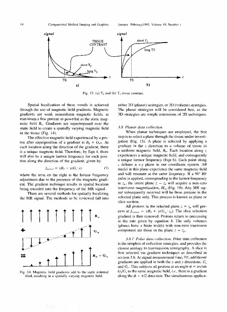
Via proper selection of TE, it is possible to obtain good contrast between various tissue types whether normal or pathological. T, and T2 tissue contrast concepts are illustrated in Fig. 13.

It has been found that pathology often exhibits T, and T2 values differing from surrounding healthy tissue.

3.7 Sputi$ localization in MR imaging This section begins a discussion of methods with

which to generate clinically useful image data by utilizing the theoretical results of the past sections. Ideally, we would like to somehow divide tissue into tiny volume elements, referred to as voxels. Voxels must have a finite volume in order to contain enough nuclei to produce a measurable signal. Voxels need not be cubic, and are often elongated rectangles. The use of cubic voxel will be assumed, without loss of generality.

14 Computerized Medical Imaging and Graphics

signal

January-February/l995, Volume 19, Number I

signal

TISSUE CONTRAST

TE TE w

a) b)

Fig. 13. (a) TZ and (b) T, tissue contrast.

Spatial localization of these voxels is achieved through the use of magnetic field gradients. Magnetic gradients are weak nonuniform magnetic fields, at maximum a few percent as powerful as the static magnetic field &. Gradients are superimposed over the static field to create a spatially varying magnetic field in the tissue (Fig. 14).

The effective magnetic field experienced by a proton after superposition of a gradient is B0 + G,x. At each location along the direction of the gradient, there is a unique magnetic field. Therefore, by Eqn 4, there will also be a unique larmor frequency for each position along the direction of the gradient, given by

.fL?!,,, = y&, + r(G, .x1. (7)

where the term on the right is the larmor frequency adjustment due to the presence of the magnetic gradient. The gradient technique results in spatial location being encoded into the frequency of the MR signal.

There are several methods for spatially localizing the MR signal. The methods to be reviewed fall into

+ Gx

B, + Gx

Fig. 14. Magnetic field gradients add to the static external filed, resulting in a spatially varying magnetic field.

either 2D (planar) strategies, or 3D (volume) strategies. The planar strategies will be considered first, as the 3D strategies are simple extensions of 2D techniques.

3.8 Plunar data collection

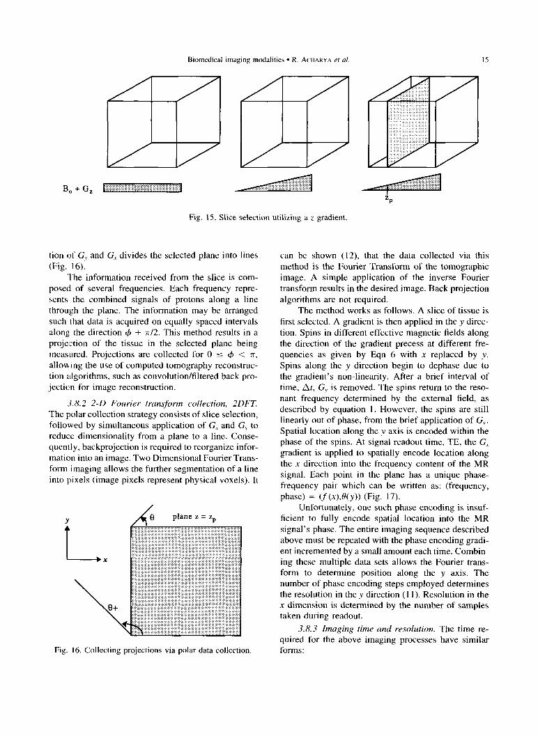
When planar techniques are employed, the first step is to select a plane through the tissue under investi- gation (Fig. 15). A plane is selected by applying a gradient in the z direction to a volume of tissue in a uniform magnetic field, BO. Each location along z experiences a unique magnetic field, and consequently a unique larmor frequency (Eqn 6). Each point along z defines a x-y plane in our coordinate system. All nuclei in this plane experience the same magnetic field and will resonate at the same frequency. If a 90” RF pulse is applied, corresponding to the larmor frequency at z,~, the entire plane z = Z, will acquire a non-zero transverse magnetization, Mxy (Fig. 10). Any MR signal subsequently received will be from protons in the selected plane only. This process is known as plane or slice section.

All protons in the selected plane z = z,, will precess at ,fLZ,nn,,r = y& + Y(G_~-z,,). The slice selection

gradient is then removed. Protons return to precessing at the rate given by equation 4. The only volumes (planes have a finite width) with non-zero transverse component are those in the plane z = z,,.

3.8.1 Polar data collection. Polar data collection is the simplest of collection strategies, and provides the closest analogy to transmission tomography. A slice is first selected via gradient techniques as described in section 3.8. At signal measurement time, TE, additional gradients are applied in both the x and y directions, G, and G,. This subjects all protons at an angle (b = arctan G,/G, to the same magnetic field, i.e., there is a gradient along the C#J + 7r/2 direction. The simultaneous applica-


Bo + G, :::.::::::.:.:;.:.. .:...:.:,: ,..... :.:.:.:.:.:.:.: I:.:::.:.::::::::::~,.: ,,.,.

Fig. 15. Slice selection utilizing a z gradient,

tion of GX and G, divides the selected plane into lines (Fig. 16).

The information received from the slice is com- posed of several frequencies. Each frequency represents the combined signals of protons along a line through the plane. The information may be arranged such that data is acquired on equally spaced intervals along, the direction 4 + 7r/2. This method results in a projection of the tissue in the selected plane being measured. Projections are collected for 0 5 4 < 7r, allowing the use of computed tomography reconstruction algorithms, such as convolution/filtered back projection for image reconstruction.

3.8.2 2-D Fourier transform collection, 2DFT.

The polar collection strategy consists of slice selection, followed by simultaneous application of G, and G, to reduce dimensionality from a plane to a line. Conse- quently, backprojection is required to reorganize information into an image. Two Dimensional Fourier Trans- form imaging allows the further segmentation of a line into pixels (image pixels represent physical voxels). It

Y 9 plane z = zp . . . . . .>. > .: . ::::::::.:.:.:.:.:::::::::., . . . ..T . .,.: >>: : ,., :I::i:j:j:::;:..:.:.:.:.~.:~~ . . ,.,,i::,:::::j:j:i:I:i:j::::::

:.::.:::::,::~:::.:i:i:I:!I:::~

t- ~~~~~~~---,

: :.::::(::,:::,::,:::::,:~:~~:~:,::;,' '..::j:j::::'::::.::.::.:::::.j.>:.,.>..,.~.:. . . . . . . . ..v. .: :...:.:.......~::.:.:::::::::j:jj:I:I:~:~:~: . . . . . . . . . ../v. .: :.:.: : . : . . . . . . . ,: . . . . . . . . . . . . . . . . . . . . . . . . . . . . . . . . . . .:........... ..,....., :.:....................~........ .' .: :::::::::.:.:::,:: :)<,:, .,

.: .: < : ,.,,:,::,:j::::::.::::::: : ;,.:.:.::: X <: >, >, ,.JCii<jj:'j :,z;: ::: : ...::.:....,.,:,)~~~ '0 v$_:::':::j::::jj:

::::............~~::.~~:.::::.,.,:,.:.:::::::: ::...~:j~:,::,,,,,:,:::,:,:,. . .,.,.:,. ,., : ,.,.:.:...: : . .:.+:.:,:,,::,;~~ : .:.. .,.,. .,.,.~,:,::::::::::::~:.':

Fig. 16. Collecting projections via polar data collection

can be shown (12), that the data collected via this method is the Fourier Transform of the tomographic image. A simple application of the inverse Fourier transform results in the desired image. Back projection algorithms are not required.

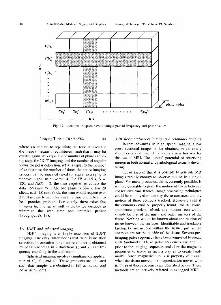
The method works as follows. A slice of tissue is first selected. A gradient is then applied in the y direction. Spins in different effective magnetic fields along the direction of the gradient precess at different frequencies as given by Eqn 6 with x replaced by y. Spins along the y direction begin to dephase due to the gradient’s non-linearity. After a brief interval of time, At, G, is removed. The spins return to the resonant frequency determined by the external field, as described by equation 1. However, the spins are still linearly out of phase, from the brief application of G,. Spatial location along the y axis is encoded within the phase of the spins. At signal readout time, TE, the G, gradient is applied to spatially encode location along the x direction into the frequency content of the MR signal. Each point in the plane has a unique phase- frequency pair which can be written as: (frequency, phase) = (f (x),0(y)) (Fig. 17).

Unfortunately, one such phase encoding is insuf- ficient to fully encode spatial location into the MR signal’s phase. The entire imaging sequence described above must be repeated with the phase encoding gradient incremented by a small amount each time. Combin- ing these multiple data sets allows the Fourier transform to determine position along the y axis. The number of phase encoding steps employed determines the resolution in the y direction (11). Resolution in the x dimension is determined by the number of samples taken during readout.

3.8.3 Imaging time and resolution. The time required for the above imaging processes have similar forms:

16 Computerized Medical Imaging and Graphics January-February/l995. Volume 19. Number I

Ine width

f(q) f(x2) f(Xj) . . . . . . . . . f(xM)

Fig. 17. Locations in space have a unique pair of frequency and phase values.

Imaging Time = TR* N* NEX. (8)

where TR = time to repetition; the time it takes for the plane to return to equilibrium such that it may be excited again. N is equal to the number of phase encoding steps for 2DFT imaging, and the number of angular views for polar collection. NEX is equal to the number of excitations; the number of times the entire imaging process will be repeated (used for signal averaging to improve signal to noise ratio). For TR = 1.5 s, N = 120, and NEX = 2, the time required to collect the data necessary to image one plane is 384 s. For 20 slices, each 1 .O mm. thick, the scan would require over 2 h. It is easy to see how imaging time could begin to be a practical problem. Fortunately, there exists fast imaging techniques as well as multislice methods to minimize the scan time and optimize patient throughput (8, 13).

3.9 3DFT and spherical imaging

3DFT Imaging is a simple extension of 2DFT imaging. The only difference is that there is no slice selection. Information for an entire volume is obtained by phase encoding in 2 directions (z and y). and frequency encoding in the x direction.

Spherical imaging involves simultaneous application of G,, G,., and G,. These gradients are adjusted such that samples are obtained in full azimuthal and polar increments.

3.10 Recent advances in magnetic resonance imaging

Recent advances in high speed imaging allow cross sectional images to be obtained in extremely short periods of time. This opens a new horizon for the use of MRI. The clinical potential of observing

motion in both normal and pathological tissue is devas- tating.

Let us assume that it is possible to generate MR images rapidly enough to observe motion in a single

plane. For many processes, this is currently possible. It

is often desirable to study the motion of tissue between

consecutive time frames. Image processing techniques could be employed to identify tissue contours, and the

motion of these contours tracked. However, even if

the contours could be properly found, and the correspondence problem solved, any motion seen would

simply be that of the inner and outer surfaces of the tissue. Nothing would be known about the motion of tissue between the surfaces. Identifiable and trackable landmarks are needed within the tissue, just as the contours are for the outside of the tissue. Several pre- imaging pulse sequences have been suggested to create such landmarks. These pulse sequences are applied

prior to the imaging sequence, and alter the magnetic properties of tissue in such a way as to create landmarks. Since magnetization is a property of tissue, when the tissue moves, the magnetization moves with it. Three of these sequences are described below. These

methods are collectively referred to as tagged MRI.

Biomedical imaging modalities l R. ACHARYA et al. 17

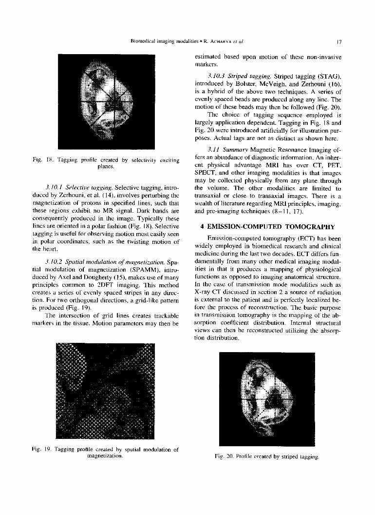
Fig. IX. Tagging profile created by selectivity exciting planes.

3.10. I Selective tugging. Selective tagging, introduced by Zerhouni, et al. (14), involves perturbing the magnetization of protons in specified lines, such that these regions exhibit no MR signal. Dark bands are consequently produced in the image. Typically these lines are oriented in a polar fashion (Fig. 18). Selective tagging is useful for observing motion most easily seen in polar coordinates, such as the twisting motion of the heart.

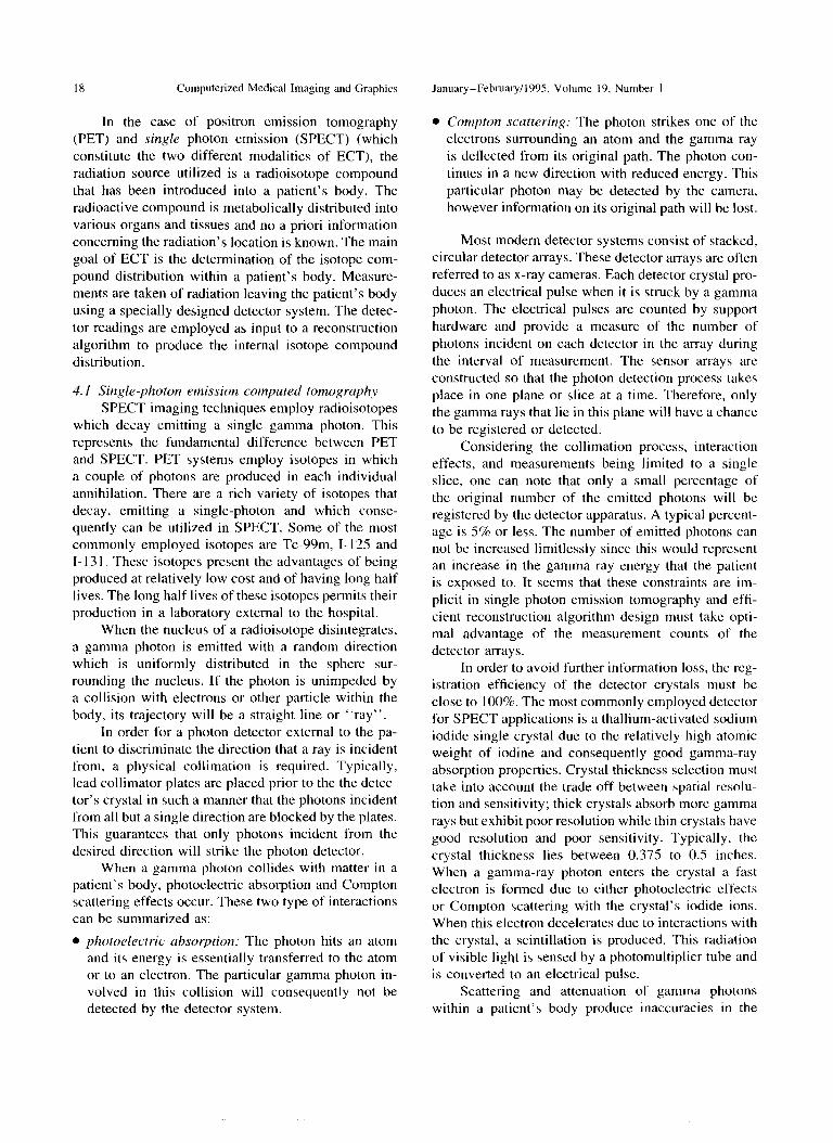
3.10.2 Spatial modulation of magnetization. Spa- tial modulation of magnetization (SPAMM), introduced by Axel and Dougherty (l5), makes use of many principles common to 2DFT imaging. This method creates a series of evenly spaced stripes in any direction. For two orthogonal directions, a grid-like pattern is produced (Fig. 19).

The intersection of grid lines creates trackable markers in the tissue. Motion parameters may then be

Fig. 19 Tagging profile created by spatial modulation of magnetization.

estimated based upon motion of these non-invasive markers.

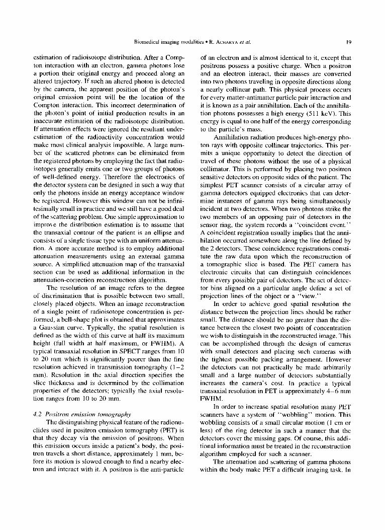
3.10.3 Striped tagging. Striped tagging (STAG), introduced by Bolster, McVeigh, and Zerhouni (16), is a hybrid of the above two techniques. A series of evenly spaced beads are produced along any line. The motion of these beads may then be followed (Fig. 20).

The choice of tagging sequence employed is largely application dependent. Tagging in Fig. 18 and Fig. 20 were introduced artificially for illustration purposes. Actual tags are not as distinct as shown here.

3. I I Summary Magnetic Resonance Imaging of- fers an abundance of diagnostic information. An inherent physical advantage MRI has over CT, PET, SPECT, and other imaging modalities is that images may be collected physically from any plane through the volume. The other modalities are limited to transaxial or close to transaxial images. There is a wealth of literature regarding MRI principles, imaging, and pre-imaging techniques (8- 11, 17).

4 EMISSION-COMPUTED TOMOGRAPHY

Emission-computed tomography (ECT) has been widely employed in biomedical research and clinical medicine during the last two decades. ECT differs fun- damentally from many other medical imaging modalities in that it produces a mapping of physiological functions as opposed to imaging anatomical structure. In the case of transmission mode modalities such as X-ray CT discussed in section 2 a source of radiation is external to the patient and is perfectly localized before the process of reconstruction. The basic purpose in transmission tomography is the mapping of the absorption coefficient distribution. Internal structural views can then be reconstructed utilizing the absorption distribution.

Fig. 20. Profile created by striped tagging.

1X Computerized Medical Imaging and Graphics January-February/1995 Volume 19. Number I

In the case of positron emission tomography (PET) and single photon emission (SPECT) (which constitute the two different modalities of ECT), the radiation source utilized is a radioisotope compound that has been introduced into a patient’s body. The radioactive compound is metabolically distributed into various organs and tissues and no a priori information concerning the radiation’s location is known. The main goal of ECT is the determination of the isotope compound distribution within a patient’s body. Measure- ments are taken of radiation leaving the patient’s body using a specially designed detector system. The detector readings are employed as input to a reconstruction algorithm to produce the internal isotope compound distribution.

4. I Single-photon emission computed tomogruphy

SPECT imaging techniques employ radioisotopes which decay emitting a single gamma photon. This represents the fundamental difference between PET and SPECT. PET systems employ isotopes in which a couple of photons are produced in each individual annihilation. There are a rich variety of isotopes that decay, emitting a single-photon and which consequently can be utilized in SPECT. Some of the most commonly employed isotopes are Tc-99m, I- 125 and I- 13 1. These isotopes present the advantages of being produced at relatively low cost and of having long half lives. The long half lives of these isotopes permits their production in a laboratory external to the hospital.

When the nucleus of a radioisotope disintegrates, a gamma photon is emitted with a random direction which is uniformly distributed in the sphere surrounding the nucleus. If the photon is unimpeded by a collision with electrons or other particle within the body, its trajectory will be a straight line or “ray”.

In order for a photon detector external to the patient to discriminate the direction that a ray is incident from, a physical collimation is required. Typically, lead collimator plates are placed prior to the the detector’s crystal in such a manner that the photons incident from all but a single direction are blocked by the plates. This guarantees that only photons incident from the desired direction will strike the photon detector.

When a gamma photon collides with matter in a patient’s body, photoelectric absorption and Compton scattering effects occur. These two type of interactions can be summarized as:

l photoelectric absorption: The photon hits an atom and its energy is essentially transferred to the atom or to an electron. The particular gamma photon in- volved in this collision will consequently not be detected by the detector system.

l Compton stuttering: The photon strikes one of the electrons surrounding an atom and the gamma ray is deflected from its original path. The photon continues in a new direction with reduced energy. This

particular photon may be detected by the camera, however information on its original path will be lost.

Most modem detector systems consist of stacked, circular detector arrays. These detector arrays are often referred to as x-ray cameras. Each detector crystal produces an electrical pulse when it is struck by a gamma photon. The electrical pulses are counted by support hardware and provide a measure of the number of photons incident on each detector in the array during the interval of measurement. The sensor arrays are constructed so that the photon detection process takes place in one plane or slice at a time. Therefore, only the gamma rays that lie in this plane will have a chance to be registered or detected.

Considering the collimation process, interaction effects, and measurements being limited to a single slice, one can note that only a small percentage of the original number of the emitted photons will be registered by the detector apparatus. A typical percentage is 5% or less. The number of emitted photons can not be increased limitlessly since this would represent an increase in the gamma ray energy that the patient is exposed to. It seems that these constraints are im- plicit in single photon emission tomography and efti- cient reconstruction algorithm design must take opti- mal advantage of the measurement counts of the detector arrays.

In order to avoid further information loss, the registration efficiency of the detector crystals must be close to 100%. The most commonly employed detector for SPECT applications is a thallium-activated sodium iodide single crystal due to the relatively high atomic weight of iodine and consequently good gamma-ray absorption properties. Crystal thickness selection must take into account the trade off between spatial rcsolu- tion and sensitivity; thick crystals absorb more gamma rays but exhibit poor resolution while thin crystals have good resolution and poor sensitivity. Typically, the crystal thickness lies between 0.375 to 0.5 inches. When a gamma-ray photon enters the crystal a fast electron is formed due to either photoelectric effects or Compton scattering with the crystal’s iodide ions. When this electron decelerates due to interactions with the crystal, a scintillation is produced. This radiation of visible light is sensed by a photomultiplier tube and is converted to an electrical pulse.

Scattering and attenuation of gamma photons within a patient’s body produce inaccuracies in the


estimation of radioisotope distribution. After a Comp- ton interaction with an electron, gamma photons lose a portion their original energy and proceed along an altered trajectory. If such an altered photon is detected by the camera, the apparent position of the photon’s original emission point will be the location of the Compton interaction. This incorrect determination of the photon’s point of initial production results in an inaccurate estimation of the radioisotope distribution. If attenuation effects were ignored the resultant underestimation of the radioactivity concentration would make most clinical analysis impossible. A large number of the scattered photons can be eliminated from the registered photons by employing the fact that radioisotopes generally emits one or two groups of photons of well-defined energy. Therefore the electronics of the detector system can be designed in such a way that only the photons inside an energy acceptance window be registered. However this window can not be infini- tesimally small in practice and we still have a good deal of the scattering problem. One simple approximation to improbe the distribution estimation is to assume that the transaxial contour of the patient is an ellipse and consists of a single tissue type with an uniform attenuation. A more accurate method is to employ additional attenuation measurements using an external gamma source. A simplified attenuation map of the transaxial section can be used as additional information in the attenuation-correction reconstruction algorithm.

The resolution of an image refers to the degree of discrimination that is possible between two small, closely placed objects. When an image reconstruction of a single point of radioisotope concentration is performed, a bell-shape plot is obtained that approximates a Gaussian curve. Typically, the spatial resolution is defined as the width of this curve at half its maximum height (full width at half maximum, or FWHM). A typical transaxial resolution in SPECT ranges from 10 to 20 mm which is significantly poorer than the fine resolution achieved in transmission tomography (l-2 mm). Resolution in the axial direction specifies the slice thickness and is determined by the collimation properties of the detectors; typically the axial resolution ranges from 10 to 20 mm.

4.2 Positron emission tomography

The distinguishing physical feature of the radionu- elides used in positron emission tomography (PET) is that they decay via the emission of positrons. When this emission occurs inside a patient’s body, the positron travels a short distance, approximately 1 mm, before its motion is slowed enough to find a nearby electron and interact with it. A positron is the anti-particle

of an electron and is almost identical to it, except that positrons possess a positive charge. When a positron and an electron interact, their masses are converted into two photons traveling in opposite directions along a nearly collinear path. This physical process occurs for every matter-antimatter particle pair interaction and it is known as a pair annihilation. Each of the annihilation photons possesses a high energy (5 11 keV). This energy is equal to one half of the energy corresponding to the particle’s mass.

Annihilation radiation produces high-energy photon rays with opposite collinear trajectories. This permits a unique opportunity to detect the direction of travel of these photons without the use of a physical collimator. This is performed by placing two positron sensitive detectors on opposite sides of the patient. The simplest PET scanner consists of a circular array of gamma detectors equipped electronics that can determine instances of gamma rays being simultaneously incident at two detectors. When two photons strike the two members of an opposing pair of detectors in the sensor ring, the system records a “coincident event.” A coincident registration usually implies that the annihilation occurred somewhere along the line defined by the 2 detectors. These coincidence registrations constitute the raw data upon which the reconstruction of a tomographic slice is based. The PET camera has electronic circuits that can distinguish coincidences from every possible pair of detectors. The set of detector bins aligned on a particular angle define a set of projection lines of the object or a “view.”

In order to achieve good spatial resolution the distance between the projection lines should be rather small. The distance should be no greater than the distance between the closest two points of concentration we wish to distinguish in the reconstructed image. This can be accomplished through the design of cameras with small detectors and placing such cameras with the tightest possible packing arrangement. However the detectors can not practically be made arbitrarily small and a large number of detectors substantially increases the camera’s cost. In practice a typical transaxial resolution in PET is approximately 4-6 mm FWHM.

In order to increase spatial resolution many PET scanners have a system of “wobbling” motion. This wobbling consists of a small circular motion (1 cm or less) of the ring detector in such a manner that the detectors cover the missing gaps. Of course, this additional information must be treated in the reconstruction algorithm employed for such a scanner.

The attenuation and scattering of gamma photons within the body make PET a difficult imaging task. In

20 Computerized Medical Imaging and Graphics January_February/l995, Volume 19, Number I

some typical chest PET scans, for example, approximately 15% of the annihilation photon pairs “headed” to a particular bin detector are registered; the rest of the photons are attenuated. If no correction approach is implemented, attenuation of photons would lead to an underestimation of the radioisotope concentration. Fortunately attenuation correction techniques can be applied. One approach consists of introducing an attenuation correction factor in the estimation of the radionuclide concentration. This correction factor is the ratio of the measurement of a detector bin when a positron-emitting source point is placed on one side of the PET scan area and a measurement taken with and without a patient in the PET scanner. A complete attenuation correction is then possible, disposing of the correction factor for all detector pairs.

The problem of scattering is more difficult to treat. If a deflected photon continues travelling in the plane of the ring detector after the scattering, this photon may still hit a detector and generate a false coincidence. A energy window approach similar to that employed for SPECT can be implemented for PET scanning. How- ever, this represents only a partial solution due to the finite accuracy in energy measurement by the scintillation crystals employed in PET. New approaches to scatter correction are currently undergoing active research.

Another factor which complicates PET is the presence of “accidental coincidences”. The detection system registers a coincidence event when both detectors of a bin are triggered within some resolving time r, which is typically measured in nsec. Usually these photons are produced by the same annihilation event. However it is possible that the system can be “tricked” by photons produced in unrelated annihilations. The rate of accidental coincidences per second N is given

by

N = 2 X T X s, X &. (9)

where S, and Sz are the counting rates of each of the detectors. The problem of accidental coincidence rapidly increases with the radionuclide concentration. The rate of counts measured by the detectors are proportional to the concentration value. The influence of accidental coincidence can be reduced by subtracting the computed number of random coincidences using the equation above.

4.3 PET reconstruction algorithms Estimation of the positron-emitter compound dis-

tribution f (x, y, 2, t) is realized through computational algorithms. These algorithms are provided the number of counts M, associated with the projection lines L,. If

the period At in which the data was collected is short enough and if we proceed to reconstruct one transaxial slice at the time, the problem reduces to the determination of the 2D functionf (x, v). The basic problem can be stated as follows:

Estimate the function ,f (x, y) from the system of equations

where L, is the i-th line of the I projection lines (detector bin lines in the PET case); c, = M,IV, depends on the attenuation line integral V, which can be either calculated from a hypothetical attenuation coefficient or from an experimental measurement.

Reconstruction algorithms can be divided into; back-projection methods, Fourier methods and iterative methods. The first two methods (transform methods) are the most commonly employed due to relative ease of implementation and low computational cost. The images obtained by transform methods are good enough for a great variety of applications. On the other hand, iterative methods provide greater flexibility in the introduction of attenuation correction information to the algorithm and statistical treatment of the data.

A simple reconstruction scheme is the back projection process. This method consists of reconstructing each transaxial slice image by a method similar to that described in section 2 for CT machines. The filter employed in this filtered back projection is typically a multiplicative combination in Fourier space of a ramp and another filter, such as the Hamming, Butterworth or Shepp-Logan filter (18).

Iterative reconstruction methods include; the alge- braic reconstruction technique (ART), the simultaneous iterative reconstruction technique (SIRT) and the least-squared iterative technique. The first two methods involve the alteration of the estimate of the transaxial image around a circle by adding or subtracting from each point to what is called for. The least-squared iterative technique is based on the minimization of the squared error which is defined as the square of the difference between the measured and calculated projection. The minimization process is performed by cal- culating the partial derivatives of the squared error with respect to variables of interest and setting this derivative equal to zero ( 19).

Shepp and Vardi have presented a reconstruction methodology based on statistical methods (20). Their method is based on the expectation maximization of the emission distribution. Shepp and Vardi take in account the Poisson statistics of radioactive decay. Con- vergency to a global maximum is guaranteed by the

Biomedical imaging modalities l R. ACHARYA et ul. 21

Shepp-Vardi algorithm. However, approaching this maximum value can be exceedingly slow in some cases.

5 BIOMAGNETIC SOURCE IMAGING WITH SQUIDS

Blomagnetic source imaging is a relatively new medical imaging modality which produces representa- tions ot’ the minute magnetic fields created by neuronal activit) within the body (I). As in the case of ECT, images produced via Biomagnetic Source Imaging provide mappings of functional rather than anatomical information. An important goal of this technology is the ability to localize neuron activity in response to specifically applied sensory stimuli (21).

Biomagnetic source imaging is made possible by a solid state sensor known as a Superconducting Quan- tum Interference Device (SQUID). SQUID sensors can be employed to measure the magnetic fields produced in the hrain by neural currents. Given a set of external magnetic measurements, it is desirable to generate a visual mapping of the current densities, in three dimen- sions, that gave rise to the external magnetic field (21). It is hoped that SQUID technology and Biomagnetic source Imaging will be of significant assistance to researchers investigating epilepsy, Alzheimer’s disease, Parkinson’s disease, and schizophrenia (1).

6 DIGITAL SUBTRACTION ANGIOGRAPHY

A common problem with the radiograph discussed in section 2 is the poor contrast between anatomical structures. This low contrast resolution limits the utility of such radiographs severely. However through the use of digital acquisition systems it is possible to greatly increase the utility of 2D projection radiographs for certain, specific applications. Digital Subtraction Angi- ography (DSA) is a modality that exploits the digital acquisition of radiographs to produce high contrast images of blood vessels.

A common problem with radiograph technology is the fact that many internal tissues are superimposed on each other. The projection nature of the radiograph yields a final image in which it is difficult to delineate individual structures. Wherein a specific structure is analyzed it would be advantageous to acquire a radiograph which displayed only that structure without any subsequent loss of resolution. This result could be achieved in a digital image if the values of all pixels without information on that structure were set to zero and all pixels corresponding to the structure of interest were allowed to maintain their natural values. While such a result could be obtained using image processing

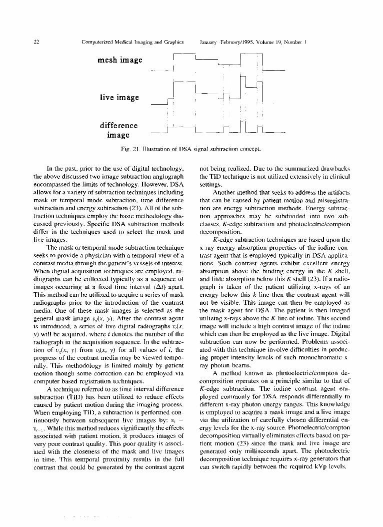
techniques, such as segmentation, the resulting loss in resolution would degrade severely an already poor contrast image. However if two images were taken of a subject, in which the contrast of the anatomical structure of interest changed significantly from one image to the next, excellent results could be achieved. The subtraction of two digital images results in a difference image. This difference image retains only the information that has changed from one image to the other. The digital subtraction of radiographs is the concept underlying DSA (22). This concept is illustrated with a ID signal in Fig. 2 1.

The basis for a DSA device consists of x-ray system very similar to that used for a conventional radiograph. The main difference occurs in the technique used to acquire the radiograph. Conventional radiography utilizes typically a film, which after processing will contain an image proportional to the amount of x-ray energy leaving the patient’s body. Subtraction angiography has been practiced employing film technology (23). However such techniques possess disad- vantages, such as the long time interval that takes place between subsequent radiographs. Patient movement during the entire radiograph acquisition sequence creates significant problems for the subtraction process since the methodology is premised on registration between the subtracted images.

In the case of DSA, the film acquisition apparatus is replaced by a system that can rapidly acquire a high resolution image of x-ray radiation incident on it. After proper patient positioning, an initial radiograph is taken of a patient. This initial radiograph is called commonly the musk image and contains the base information that will be subtracted from the second image. The mask radiograph is acquired and stored in a computer. A contrast medium is then injected into the patient. This contrast medium is designed to elicit a significant change in the contrast of blood in the vessels of interest. A second radiograph is then taken of the patient with the contrast agent in place. This second image is again acquired and stored in a computer’s memory. This image is referred to as the live image in that it contains vessel information that was not present in the mask image. The digital results of these radiographs can now be subtracted and their difference amplified. After subtraction, all information that was in both the mask and live images has been eliminated. The resulting image is now a high contrast image of the patient’s blood vessels in a region of interest. Clinical applications of DSA differ in some ways from the simplistic description above. However such techniques utilized for the improvement of image quality do not affect the underlying methodology described herein.

22 Computerized Medical Imaging and Graphics January-February/l995, Volume 19. Number I

mesh image ::

live image J---y n]r

difference

image

: : :

Fig. 21. Illustration of DSA signal subtraction concept.

In the past, prior to the use of digital technology, the above discussed two image subtraction angiograph encompassed the limits of technology. However, DSA allows for a variety of subtraction techniques including mask or temporal mode subtraction, time difference subtraction and energy subtraction (23). All of the subtraction techniques employ the basic methodology discussed previously. Specific DSA subtraction methods differ in the techniques used to select the mask and live images.

The mask or temporal mode subtraction technique seeks to provide a physician with a temporal view of a contrast media through the patient’s vessels of interest. When digital acquisition techniques are employed, radiographs can be collected typically as a sequence of images occurring at a fixed time interval (at) apart. This method can be utilized to acquire a series of mask radiographs prior to the introduction of the contrast media. One of these mask images is selected as the general mask image u,~(x, y). After the contrast agent is introduced, a series of live digital radiographs u,(x, y) will be acquired, where i denotes the number of the radiograph in the acquisition sequence. In the subtraction of u,(x, y) from U&Y, y) for all values of i, the progress of the contrast media may be viewed tempo- rally. This methodology is limited mainly by patient motion though some correction can be employed via computer based registration techniques.

A technique referred to as time interval difference subtraction (TID) has been utilized to reduce effects caused by patient motion during the imaging process. When employing TID, a subtraction is performed continuously between subsequent live images by: u, - u,_, While this method reduces significantly the effects associated with patient motion, it produces images of very poor contrast quality. This poor quality is associated with the closeness of the mask and live images in time. This temporal proximity results in the full contrast that could be generated by the contrast agent

not being realized. Due to the summarized drawbacks the TID technique is not utilized extensively in clinical settings.

Another method that seeks to address the artifacts that can be caused by patient motion and misregistra- tion are energy subtraction methods. Energy subtraction approaches may be subdivided into two sub- classes, K-edge subtraction and photoelectric/compton decomposition.

K-edge subtraction techniques are based upon the x-ray energy absorption properties of the iodine contrast agent that is employed typically in DSA applications. Such contrast agents exhibit excellent energy absorption above the binding energy in the K shell, and little absorption below this K shell (23). If a radiograph is taken of the patient utilizing x-rays of an energy below this k line then the contrast agent will not be visible. This image can then be employed as the mask agent for DSA. The patient is then imaged utilizing x-rays above the Kline of iodine. This second image will include a high contrast image of the iodine which can then be employed as the live image. Digital subtraction can now be performed. Problems associated with this technique involve difficulties in producing proper intensity levels of such monochromatic x- ray photon beams.

A method known as photoelectric/compton decomposition operates on a principle similar to that of K-edge subtraction. The iodine contrast agent employed commonly for DSA responds differentially to different x-ray photon energy ranges. This knowledge is employed to acquire a mask image and a live image via the utilization of carefully chosen differential energy levels for the x-ray source. Photoelectric/compton decomposition virtually eliminates effects based on patient motion (23) since the mask and live image are generated only milliseconds apart. The photoelectric decomposition technique requires x-ray generators that can switch rapidly between the required kVp levels.


The major practical difference between the two energy subtraction based techniques discussed is the requirements they place on the employed x-ray genera- tor. K-edge subtraction requires difficult to produce, monochromatic x-ray beams while the photoelectric subtraction approach employs beams of differing ener- gies. While the decomposition approach utilizes easier to produce x-ray beams, it has the disadvantage of a reduction in output signal to noise ratio for low kVp x-rays. This drawback is due to the significant attenuation of the low energy beams by thicker structures in the patient.

7 ULTRASOUND IMAGING

UI trasound based imaging techniques comprise a set of methodologies capable of acquiring both quantitative and qualitative diagnostic information. Many ultrasound based methods are attractive due to their ability to obtain real time imagery employing compact and mobile equipment at a significantly lower cost than is incurred with other medical imaging modalities. The real time nature of ultrasound makes it possible for physicians to observe the motion of structures inside a patient’s body. This ability has resulted in the wide- spread use of ultrasound technology in the fields of pediatrics and cardiology. Equipment which employs doppler echo techniques can extract quantitative velocity information such as the rate of blood flow in a vessel of interest. Additionally, the introduction of ultrasound signals into a patient at the levels currently employed has been determined to be very safe (2). The lack of negative exposure effects, portability, relatively low cost and quantitative acquisition modes makes ultrasound techniques an important class of medical imaging methods.

Ultrasound is classified as sound waves possessing a high temporal frequency. Typical medical instruments for diagnostic ultrasound employ waveforms that oscillate in the range of I-1OMHz. (2). Such waves can be produced using a single ultrasound transducer or an array of transducers. Ultrasound transducers are capable of producing ultrasound signals when they are excited electrically. Inversely, these transducers produce an electric signal when excited by incident ultrasound rays. Consequently, the same set of ultrasound transducers are typically used for both ultrasound transmission and detection in medical applications.

The sound waves transmitted by the ultrasound transducers are introduced into the patient’s body in the area of diagnostic interest. As the waves pass through the body they travel through differing tissue

types with correspondingly differing acoustic properties. At the boundary between two tissues types a partial reflection of the ultrasound signal will take place. Some portion of the sound waves will be reflected back towards the source transmitter while the remaining portion of the incident ultrasound will continue propagating onwards. This process is not idealized in living tissue and results in complex scattering interactions that are out of the scope of this paper. Reflected waveforms are measured with respect to their time of original transmission by employing the source transducer apparatus as mentioned above. It should be intuitively clear that only waveforms reflected along the incident path will be detectable by the original transducer.

It has been previously mentioned that ultrasound source/detector configurations can consist of a single transducer or an array of transducers. Array transducers arrangements are often employed in modem medical ultrasound units. These array configurations provide a larger receptor aperture and subsequently improved image reconstruction.

In order to understand the manner in which ultrasound machines acquire images it is best to first investi- gate a simple, idealized scenario. One such case might be a task that entails imaging a 1D scene consisting of a single, ideal reflector using a single transmitter located at the origin. If an ultrasound pulse is transmitted at time I, and a return pulse is detected at time t2 then the distance to the target from the transmitter may be calculated as

t2 - II x=- c

(11)

where c is the speed of sound in the instant medium. Extending this approach to medical applications, one can view the body as a series of point sources located at the junctions of tissues with differing characteristic acoustic impedances. Ultrasound units designed to image internal structures for applications such as echo- graphic and in pediatric settings are designed to measure the time of reception of ultrasound signals with respect to their time of transmission in real time. This results in the real time measurement of the distance from the transducer to internal anatomical surfaces, resulting in real time imagery of these structures.

Information from returned echoes or reflections with respect to time can be presented to the physician in several ways (2). Two commonly employed techniques are time amplified and brightness mode displays. Time amplified or A mode displays present the amplitudes of the returned ultrasound signals with respect to their time of return as a series of ID spikes of varying height. Brightness or B mode displays pres-

24 Computerized Medical Imaging and Graphics JanuaryFebruary/l995. Volume 19, Number I

ent the same data on a single line. The brightness of each point on this line indicates the signal amplitude detected at that time or depth. If an array of detectors are employed with the proper mechanisms then it is possible to generate a series of B mode scan lines. The combination of these scan lines results in a 2D fan like view. This 2D view can be generated in real time allowing for the detection and viewing of moving internal structures such as a beating heart. Another mode of image presentation commonly referred to is time motion or M mode. M mode employs a display of B mode lines with respect to a time axis acquired by moving the source/transmitter wand across the area of interest (24).

Quantitative information can be extracted from echo reflections through an understanding and utilization of the Doppler effect. In short, when a signal with frequency .fo and propagating at speed u, is reflected from a target moving at a speed u, then the frequency of the echoed signal received at the ultrasound detector is shifted by a factor described by the Doppler principle. The frequency of the transmitted wave is shifted by a factor of

f d

_ 2v,fu v,

(12)

where fd is the approximate, detected doppler frequency shift and fr = fd + ,fo, where fr is the actual frequency received at the detector.

An area in which Doppler techniques are commonly employed is Doppler Echocurdiogruphy. Dopp- ler Echocardiography allows the measurement of the velocity and direction of blood flow at a fixed distance from the ultrasound transducer within a patient’s body. The Doppler shifted frequencies to be measured are produced by the reflection of injected ultrasound waves from flowing red blood cells in the vessels of interest. When utilizing the method of pulsed Doppler echocardiography, short bursts of ultrasound are introduced into the patient. Pulsed echo techniques keep the target distance fixed and retrieve velocity measurements for targets located at that distance. Since the desired distance of measurement is fixed, the expected echo time is also fixed. Echoes not received in a neighborhood of this expected echo time are not processed by the imaging instrumentation. This technique is often referred to as range gating (2). An alternative Doppler technique is continuous wave Doppler. When this method is employed, ultrasound is continuously injected into the patient. Such an approach is advantageous in that it allows for very accurate, high velocity measurements. Unfortunately, when continuous Dopp- ler is employed the depth at which the velocity is being

measured cannot be determined due to the fact that no range gating takes place. For either of the Doppler principle based techniques, the echoed signal’s frequency components are measured so as to determine the Doppler frequency shift using the fast fourier transform (FFT).

8 CONCLUSION

Advancing technology is increasing steadily the radiologist’s ability to learn accurate and precise information about a patient in a non-invasive manner. Cur- rent medical imaging modalities are capable of acquiring data on internal anatomical structures, as well as mappings of physiological function. Advanced soft- ware reconstruction algorithms and analytic techniques seek to maximize the information derived from current medical modalities while driving the development of even more advanced technologies.

An overview has been provided of some of the more popular medical imaging modalities currently in clinical use. It is hoped that a general understanding of the modality from which an image is derived will help researchers in the subsequent analysis of the image data.

1.

2.

3.

4.

5.

6.

7.

8.

9.

IO.

I I.

12.

REFERENCES

Biomagnetic source imaging with squids: A new method for functional brain diagnosis. Cryogenic News X):740; August 1990. Geiser. E.A.; Oliver, L.H. Echocardiography: Physics and instrumentation. In: Collins, SM.; Skorton, D.J., eds. Cardiac imaging and image processing. New York: McGraw-Hill; 1986: 3-23. Sprawls. P. The principles of computed tomography, image formation and quality. In: Gedgaudas-McClees, R.K.; Torres, W.E., eds. Essentials of body computed tomography. Philadelphia: W.B. Saunders Company; 1990. Jain, A.K. Fundamentals of digital image processing. New Jer- sey: Prentice Hall: 1989. Robb, R.A.; et al. High speed 3d x-ray ct: The dynamic spatial reconstructor. Proceedings of the IEEE, 7 I (3):308-3 19; March 1983. Acharya, R.S.; et al. High speed 3d imaging of the beating heart using temporal estimation. Comput. Vision Graph. Image Process. 259-270; September 1987. Boyd, D.P.; Farmer, D.W. Cardiac computed tomography. In: Collins. SM.; Skorton, D.J., eds. Cardiac imaging and image processing. New York: McGraw-Hill; 1986. Edelman. R.R.; Hesselink, J.R. Clinical magnetic resonance imaging. Toronto: W.B. Saunders Co.; 1990.- Stark. D.D.: Bradlv. W.G. Jr. Magnetic resonance imaging. 2nd ed. Toronto: Mosby-Year Book; 1992.

- -

Kean, D.; Smith, M. Magnetic resonance imaging. Williams and Wilkins; 1986. Chakeres, D.W.; Schmalbrock. P. Fundamentals of magnetic resonance imaging. Baltimore: Williams and Wilkins; 1992. King, K.F.; Moran, P.R. A unified description of nmr imaging, data-collection strategies and reconstruction. Medical physics. I I ( I ); Jan/Feb 1984.

Biomedical imaging modalities l R. ACHARYA et crl. 25

13.

14.

IS.

16.

17.

IX.

I’).

20.

21.

22.

23.

24.

Riederer. S. Recent advances in magnetic resonance imaging. Proceedings of the IEEE, 76(9); September 198X. Zerhouni, E.A.; et al. Human heart: Tagging with mr imaging- A method for noninvasive assessment of myocardial motion. RadIology 169:59-63; 1988. Axel, L.; Dougherty, L. MR imaging of motion with spatial modulation of magnetization. Radiology I7 I :X4 I -X45; 1989. Bol\ter, B.D.; McVeigh, E.R.; Zerhouni, E.A. Myocardial tagging in polar coordin&es with use of striped tags. Radiology 17:’ 769-772; 1990. Oldt~ndorf, W.H.; Oldendorf, W. Jr. Basics of magnetic resonance imaging. Boston: Martinus Nijhoff; 1988. Herman, G.T. Image reconstruction from projections: implementation and applications. New York: Academic Press; 1980. BucJlnger; Gullberg. Three-dimensional reconstruction in nu- cle.lr medicine emission imaging. IEEE Transactions on nuclear science, 21:2-20; 1974. Shcpp, L.A.; Vardi, Y. Maximum likelihood reconstruction for emitsion tomography. IEEE Transactions on medical imaging. Ml-l(2):] 13-121; October 1982. Mcsher, J.C.: Lewis. P.S.; Leahy, R.M. Multiple dipole model- ing .md localization from spatio-temporal meg data. IEEE Trans- actIons on Biomedical Engineering, 39(6):541-559; June 1992. Kruger, R.A.; Riederer. S.J. Basic concepts of digital subtraction anglography. Boston: G.K. Hall Medical Publishers; 1984. Vill.lfana, T. Basic physics and instrumentation for digital sub- tractlon angiography. In Faerber, E.N., ed. Digital subtraction imaging in infants and children. Mount Kisco, New York: Futura Publishing Company, Inc.; 1989: I-36. Feipenbaum, H. Echocardiography. Lea and Febiger. Philadel- phia. 5th edition, 1994.

About the Author-RAJ ACHARYA obtained his Ph.D from the Universlry of Minnesota/Mayo Graduate School of Medicine in 1984

and is currently an Associate Professor of Electrical and Computer Engineering at SUNY-Buffalo. He worked with the Dynamic Spatial Reconstructor project at the Mayo Clinic from 19X I - 1985 and was a research scientist at GE-CGR in Paris, France during 1984 to 1986. He is presently the Director of SUNY Buffalo’s Biomedical Imaging Group (BMIG). He is a member of the editorial board of the Journal of Computerized Medical Imaging and Graphics as well as Cochair of the 1994 IEEE Workshop in Biomedical Image Analysis. He has also served as the General Chair of the SPIE Conference on Biomedi- cal Image Processing in both 1992 and 1993, and is currently the General Chair of the 1994 SPIE International Conference on Physiol- ogy and Function from Multidimensional Images.

About the Author-RICHARD WASSERMAN is currently working towards his doctorate in electrical engineering at the University of Buffalo. His research interests include the application of data fusion techniques to multimodality imaging as well as applications in the field of radiation therapy treatment planning.

About the Author-JEFFRw STEVENS was born in Buffalo, New York on January 25, 1970. He received his B.S.IM.S. degrees in electrical engineering from the State University of New York at Buffalo. in 1992 and 1994. respectively. His research interests are in the areas of image processing and computer vision.

About the Author-CARLos M. HIN~J~SA was born in Monterrey, Mexico, on September 23. 1964. He received the B.Sc. degree in physics with honors from Instituto Tecnologico de Monterrey (1.T.E.S.M) in 1985 and the M.S.E. in digital control from the same university in 1990. He was an Assistant Professor of the Department of Physics and a researcher in the Center of Optics in the I.T.E.S.M. He is presently working towards the PhD degree in electrical engineering at the State University of New York (S.U.N.Y.) at Buffalo. His current research interests include reconstruction for emission tomography and integration of different medical imaging modalities.

Date post:	27-Feb-2023
Category:	Documents
Upload:	independent
View:	1 times
Download:	0 times

Bio medical Imaging

Documents