A.-L. Jousselme, P. Maupin / International Journal of Approximate Reasoning 53 (2012) 118–145 119
In fuzzy set theory, Bloch proposed a detailed survey of distances between fuzzy sets in [8] where fuzzy distances
are reviewed and classified with respect to the needs in image processing applications. In the framework of imprecise
probabilities, Abellán and Gómez [1] defined three measures for comparison of credal sets 1 : an inconsistency measure, an
inclusion index and an informative distance. In [10], de Campos et al. proposed a method for building distances between
fuzzy measures based on associated probability distributions. In possibility theory, Jenhani et al. defined in [34] a distance
between possibility distributions together with some required properties.
In recentyears,manyworksonmeasuring thedistancebetweenbelief functionshaveemerged. Fora long time,Demspter’s
conflict factor has been the onlyway to quantify the interaction between belief functions (see for example [54,23]). However,
this factor may not be appropriate to quantify the dissimilarity between two belief functions as the conflict between two
identical belief functions may not equal to 0, a result somewhat counterintuitive. Several approaches have been proposed
for the definition of distances in evidence theory. In [56,46], Perry and Stephanou extended the Kullback-Liebler divergence
for probability distributions, Blackman and Popoli [7] and Ristic and Smets [50] defined a distance based on Dempster’s
conflict factor. Other authors proposed geometrical (Euclidean) distances: Fixsen and Mahler [26] defined a classification
miss-distance, Jousselme et al. [35] proposed a geometric distance accounting for the similarity between focal sets, Cuzzolin
[14] defined an Euclidean measure between belief values and extended it to Lp Minkowski measures in [16], Wen proposed
to quantify the similarity as the cosine measure of the angle between two mass vectors [59].
In the technical literature, two main aims may be identified regarding the practical use of distances between belief
functions: (1) for algorithm evaluation or optimization, for example in classification algorithms [26,35,19], or in belief
functions approximation algorithms [57,3,14,20], or for combination ruleparameter estimation [21,48,61], (2) as adefinition
of agreement between sources of information, for example in clustering techniques [4,60,5,52], or as a basis for discounting
factors [43,29,12,31,38,45]. In algorithm evaluation or optimization, the distance is computed with respect to a reference
belief function Belr or to an entire reference space, as in works on approximation algorithms where distances are measured
with respect to the subspace of Bayesian or consonant belief functions ([13] for instance), whereas in the definition of
agreement between sources of information no such reference exists. Depending on the application, some formal properties
are requiredwhile some others are superfluous. Our position is that none of the distancemeasures can be said to be superior
to the others in the absolute and that the choice of such a measure should always be guided by practical considerations
relative to a specific application.
In Section 2, we review important basic notions of evidence theory, including notational conventions that will ease the
subsequent analytic exposition, together with an emphasis on the geometrical interpretation in Section 2.2. The properties
of similarity and dissimilaritymeasures are detailed in Section 2.3. A categorization of the distances is proposed in Section 3,
based on the definition a set of different inner-products between belief functions. It is shown that most of the existing mea-
sures can fit in this general formulation. We also mention other works of interest. In Section 4, we discuss some outcomes
of the present survey: Section 4.1 summarizes the existing measures and proposes new measures, Section 4.2 discusses
the metric and structural properties, the normalization factors are presented in Section 4.3, Bayesian belief functions are
discussed in 4.4, Section 4.5 hightlights two kinds of measures that are metric distances and angles, an alternative to Demp-
ster’s rule is proposed in Section 4.6, different encoding of belief functions are proposed in Section 4.7 and some comments
about extensions to unnormalized and fuzzy belief functions are provided in Section 4.8. An experimental comparison of
distance measures is proposed in Section 5 firstly based on a toy example (Section 5.1) and on a more semantic approach
using additive trees (Section 5.2). Section 6 concludes on future works that will be developed in upcoming publications.
2. Background
The background material presented in this section deals with the following four main points: (1) the geometrical inter-
pretation of belief functions, that will be used in this paper to ease the exposition, (2) definitions on similarity, dissimilarity
andmetric measures, (3) basic notions on inner products and distances, and (4) the structural properties of belief functions.
2.1. Basics on evidence theory
Let X be a frame of discernment containing N distinct objects xi, i = 1, . . . ,N. We denote by x an element of X . The
power set of X , denoted by 2X , is the set of the 2N subsets of X . A Basic Probability Assignment (BPA) m is a mapping from
2X to [0, 1] satisfying the two following conditions:∑A⊆X
m(A) = 1 and m(∅) = 0 (1)
A subset A of X is called a focal element if m(A) > 0 and we denote by F the set of all the focal elements, i.e. F = {A ⊆X|m(A) > 0}. Three one-to-onemappings can be defined fromm, namely the belief, plausibility and commonality respectively
for all A ⊆ X:
1 A credal set K is a closed and convex set of probability distributions. The credal set associated with a belief function Bel defined on a frame of discernment
X is K = {p|Bel(A) ≤ p(A),∀A ⊆ X}.
120 A.-L. Jousselme, P. Maupin / International Journal of Approximate Reasoning 53 (2012) 118–145
Bel(A) = ∑B⊆A
m(B), Pl(A) = ∑B∩A �=∅
m(B), q(A) = ∑A⊆B
m(B) (2)
The pignistic probability [55] is defined for all A of X by:
Bet P(A) = ∑B⊆X
m(B)|A ∩ B|
|B| (3)
where |A| is the cardinality of set A. In particular, if A is a singleton {x}, we have Bet P({x}) = ∑x∈B
m(B)|B| .
Let us introduce the following indexes between two subsets of X:
Inclusion index : Inc(A, B) = 1 if A ⊆ B and 0 otherwise (4)
Intersection index : Int(A, B) = 1 if A ∩ B �= ∅ and 0 otherwise (5)
Pignistic index : Bet(A, B) = |A ∩ B||B| (6)
The Inc index corresponds to QfrM in [53]. We note that Int is symmetric while Inc and Bet are not. The dual index of Int is
1 − Int which is such that 1 − Int(A, B) = 1 iff A ∩ B = ∅ and 0 otherwise. Introducing these indexes allows alternative
notations for Eqs. (2) and (3):
Bel(A) = ∑B⊆X
m(B)Inc(B, A) (7)
Pl(A) = ∑B⊆X
m(B)Int(A, B) (8)
q(A) = ∑B⊆X
m(B)Inc(A, B) (9)
Bet P(A) = ∑B⊆X
m(B)Bet(A, B) (10)
2.2. A geometrical interpretation of evidence theory
The geometrical interpretation of evidence theory can be traced back to the work of Ronald Mahler in 1996 [42], where
the author sets the bases with a random sets interpretation of belief functions. 2 This interpretation has also been used in
[35] to define a distance between two belief functions, and further developed by Cuzzolin in [14,15] for instance.
Let EX be the 2N-dimensional Cartesian space spanned by the set of vectors {eA, A ⊆ X}. Any vector v of EX can be then
written as v = ∑A⊆X αAeA, where αA ∈ IR is the coordinate of v along the dimension eA.
A BPA is a vector 3 m of EX satisfying the properties (1), i.e.∑
A⊆X αA = 1, α∅ = 0, with αA ≥ 0 together with
αA = m(A). A belief function Bel is then represented equivalently by a vector Bel = ∑A⊆X Bel(A)eA, with its belief values
Bel(A) as coordinates of Bel. Equivalent representations hold for Pl and q.
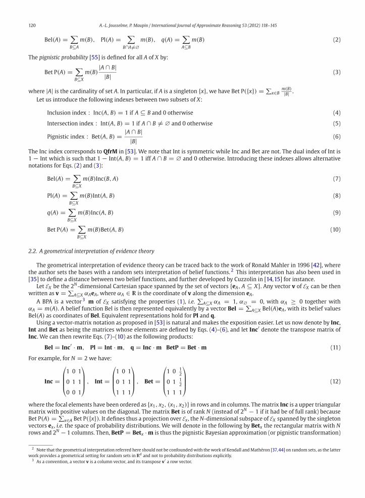
Using a vector-matrix notation as proposed in [53] is natural and makes the exposition easier. Let us now denote by Inc,
Int and Bet as being the matrices whose elements are defined by Eqs. (4)–(6), and let Inc′ denote the transpose matrix of
Inc. We can then rewrite Eqs. (7)–(10) as the following products:
Bel = Inc′ · m, Pl = Int · m, q = Inc · m BetP = Bet · m (11)
For example, for N = 2 we have:
Inc =
⎛⎜⎜⎜⎝1 0 1
0 1 1
0 0 1
⎞⎟⎟⎟⎠ , Int =
⎛⎜⎜⎜⎝1 0 1
0 1 1
1 1 1
⎞⎟⎟⎟⎠ , Bet =
⎛⎜⎜⎜⎝1 0 1
2
0 1 12
1 1 1
⎞⎟⎟⎟⎠ (12)
where the focal elements have been ordered as {x1, x2, (x1, x2)} in rows and in columns. Thematrix Inc is a upper triangular
matrix with positive values on the diagonal. The matrix Bet is of rank N (instead of 2N − 1 if it had be of full rank) because
Bet P(A) = ∑x∈A Bet P({x}). It defines thus a projection over Ex , theN-dimensional subspace of EX spanned by the singleton
vectors ex , i.e. the space of probability distributions. We will denote in the following by Betx the rectangular matrix with N
rows and 2N − 1 columns. Then, BetP = Betx ·m is thus the pignistic Bayesian approximation (or pignistic transformation)
2 Note that the geometrical interpretation referred here should not be confoundedwith thework of Kendall andMathéron [37,44] on random sets, as the latter
work provides a geometrical setting for random sets in IRd and not to probability distributions explicitly.3 As a convention, a vector v is a column vector, and its transpose v′ a row vector.
A.-L. Jousselme, P. Maupin / International Journal of Approximate Reasoning 53 (2012) 118–145 121
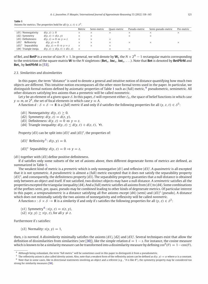
Table 1
Axioms for metrics. The properties hold for all (y, z, t) ∈ S3.
of Bel, and BetP is a vector of size N × 1. In general, we will denote byWx the N × 2N − 1 rectangular matrix corresponding
to the restriction of the squarematrixW to the N singletons (Betx, Incx, Intx, . . .). Note that Bet is denoted by BetPfrM and
Betx by betPfrM in [53].
2.3. Similarities and dissimilarities
In this paper, the term “distance” is used to denote a general and intuitive notion of distance quantifying howmuch two
objects are different. This intuitive notion encompasses all the other more formal terms used in the paper. In particular, we
distinguish formal notions defined by axiomatic properties of Table 1 such as (full) metric, 4 pseudometric, semimetric. All
other distances satisfying less axioms than a premetric will be called nonmetric.
Let y be an element of a given space S . In this paper, S will represent either EX , the space of belief functions in which case
y ≡ m, or 2X , the set of focal elements in which case y ≡ A.
A function d : S × S → IR is a (full) metric if and only if d satisfies the following properties for all (y, z, t) ∈ S3:
(d1) Nonnegativity: d(y, z) ≥ 0.
(d2) Symmetry: d(y, z) = d(z, y).(d3) Definiteness: d(y, z) = 0 ⇔ y = z.
(d4) Triangle inequality: d(y, z) ≤ d(y, t) + d(z, t), ∀t.Property (d3) can be split into (d3)’ and (d3)”, the properties of:
(d3)’ Reflexivity 5 : d(y, y) = 0.
(d3)” Separability: d(y, z) = 0 ⇒ y = z,
(d1) together with (d3) define positive definiteness.
If d satisfies only some subsets of the set of axioms above, then different degenerate forms of metrics are defined, as
summarized in Table 1.
The weakest kind of metric is a premetricwhich is only nonnegative (d1) and reflexive (d3)’. A quasimetric is all excepted
that it is not symmetric. A pseudometric is almost a (full) metric excepted that it does not satisfy the separability property
(d3)”, and consequently, the definiteness property (d3). The separability property guaranties that a null distance is obtained
only between an object and itself. If not satisfied, two distinct objects may have a null distance. A semimetric satisfies all the
propertiesexcepted the triangular inequality (d4).Anda (full)metric satisfiesall axioms from(d1) to (d4). Somecombinations
of the prefixes semi, pre, quasi, pseudomay be combined leading to other kinds of degenerate metrics. Of particular interest
in this paper, a semipseudometric is a distance satisfying all five axioms except (d4) (semi) and (d3)” (pseudo). A distance
which does not minimally satisfy the two axioms of nonnegativity and reflexivity will be called nonmetric.
A function s : S × S → IR is a similarity if and only if s satisfies the following properties for all (y, z) ∈ S2:
(s1) Symmetry6 : s(y, z) = s(z, y),(s2) s(y, y) ≥ s(y, z), for all y �= z.
Furthermore if s satisfies:
(s3) Normality: s(y, y) = 1,
then, s is normed. A dissimilarity minimally satisfies the axioms (d1), (d2) and (d3)’. Several techniques exist that allow the
definition of dissimilarities from similarities (see [30]), like the simple relation d = 1 − s. For instance, the cosine measure
which is known to be a similaritymeasure can be transformed into a dissimilaritymeasure by defining cosd(θ) = 1−cos(θ).
4 Although being redundant, the term “full metric” will be sometimes used in this paper to distinguish it from a pseudometric.5 The reflexivity axiom is also called identity axiom. Also, note that a weakest form of the reflexivity axiom can be defined as d(y, y) = α where α is a constant.6 Note that in some cases, like in directional statements involving an object and a referent (e.g. , “A is like B”), the symmetry property may be considered too
strong for similarity measures [58].
122 A.-L. Jousselme, P. Maupin / International Journal of Approximate Reasoning 53 (2012) 118–145
2.4. Inner products and distances
An inner product ⊗ over a linear space V is a mapping
⊗ : V × V −→ IR
(v1, v2) �−→ ⊗(v1, v2) = α
which must satisfy the 3 following axioms for all vectors v1, v2, v3 of V and all scalars a, b ∈ IR:
(ip1) Symmetry: ⊗(v1, v2) = ⊗(v2, v1),(ip2) Linearity in the first argument: ⊗(av1 + bv2, v3) = a ⊗ (v1, v3) + b ⊗ (v2, v3),(ip3) Positive-definiteness: ⊗(v, v) ≥ 0 with equality only for v = 0.
A linear space V endowed with an inner product ⊗ is called an inner product space. This is true for EX in particular.
A general representation for an inner product is:
⊗W (v1, v2) = v′1Wv2 (13)
where W is a matrix of weights (weighting matrix) required to be symmetric and positive definite. 7 The angle between v1and v2 is given by:
θ = arccos
( ⊗W (v1, v2)
‖v1‖W .‖v2‖W
)(14)
where the norm of a vector v is defined as ‖v‖W = √⊗(v, v) and represents the length of v. The norm can be used to define
a distance function on EX by:
d(v1, v2) = ‖v1 − v2‖W =√
(v1 − v2)′W(v1 − v2) (15)
An inner product is degenerate if it satisfies all the properties except the separability property, i.e. if ‖v‖W = 0 does not
imply v = 0. In this case,W is only positive semidefinite. The induced norm is then a pseudonorm and the induced distance,
a pseudometric (see Table 1).
If W is square, symmetric and positive definite, then W can be uniquely factorized as W = U′U, where U is upper
triangular with positive diagonal entries (Cholesky decomposition). Note that this result also holds wheneverW is positive
semidefinite. Then, we can write (13) and (15), respectively as:
⊗(v1, v2) = (Uv1)′(Uv2) (16)
and
d(v1, v2) =√
(U(v1 − v2))′ U(v1 − v2) (17)
2.5. Structural property of belief functions
Besides the axioms introduced in the previous section, a distance between belief functions should satisfy other properties
very specific to the nature of belief functions. Although the development of such properties is out of the scope of the present
paper, we will however consider the following properties:
(sp1) Strong structural property (interaction between focal elements):
A distance measure d between two belief functions Bel1 and Bel2 is said to be strongly structural if its definition
accounts for the interaction between the focal elements of Bel1 and Bel2, i.e. if s(eA, eB), where s quantifies the
interaction between the basis vectors, plays a role in the definition of d.
(sp2) Weak structural property (cardinality of focal elements):
A distance measure d between two belief functions Bel1 and Bel2 is said to be weakly structural if its definition
accounts for the cardinality of the focal elements of Bel1 and Bel2, i.e. if |A| plays a role in the definition of d.
(sp3) Structural dissimilarity (interaction between sets of focal elements):
A distance measure d between two belief functions Bel1 and Bel2 is said to satisfy the structurally dissimilarity
property if its definition accounts for the interaction between the sets F1 and F2 of focal elements of Bel1 and
Bel2, i.e. if dfe(F1,F2), where dfe quantifies the interaction between the sets of focal elements.
7 A matrix is positive definite iff all its eigenvalues are strictly positive (λi > 0), and it is positive semidefinite iff its eigenvalues are positive (λi ≥ 0).
A.-L. Jousselme, P. Maupin / International Journal of Approximate Reasoning 53 (2012) 118–145 123
Fig. 1. Historical contributions to the measurement of distance between two belief functions.
Indeed, compared to traditional spaces, the basis vectors eA, A ⊆ X , of the space EX of belief functions can be linked
through some similarity or dissimilarity measures, making this space in some sense “curved”. For instance, the basis vectors
eA and eB where A = {x1, x2, x3} and B = {x1, x2} are more similar than the basis vectors eA and eC where C = {x4, x5}.This structural property is an interesting property to be satisfied by a distance measure between belief functions and will
be considered in the upcoming analysis as the axiomatic metric properties will be.
2.6. Notations
In the remaining of this paper, we will denote by d a dissimilarity measure, by s a similarity measure, by ⊗ an inner
product, and by cos a cosine measure. Moreover, a subscript W will be added to the previous ones to specify the weighting
matrix. A superscript s or dwill be added to ⊗ to specify ifW defines a similarity or dissimilarity respectively. A superscript
(p) will also be added to d to denote the Minskowski family, p ∈ {1, 2, . . . , ∞}.
3. Survey of the main distances in evidence theory and classification
Since the introduction of Dempster’s conflict measure [17], about 20 distance measures between belief functions have
been defined in the technical literature. Fig. 1 summarizes several contributions that will be reviewed in this paper.We hope
this survey is exhaustive and apologize for any forgotten contribution.
Most of the distance measures defined so far in the evidence theory framework are derived from inner products, either
directly (see Section 3.3), or through metrics. The main family of metrics considered is the Minkowski family (Section 3.2),
denoted as Lp, whosemost famous representative is the Euclideanmetric family L2 (see Section3.2.2). L1 metrics (Manhattan)
and L∞ metrics (Chebyshev norm, also called infinity, uniform or supremum norm) will be reviewed in Sections 3.2.1 and
3.2.3 respectively. The Fidelity family of distances will be described in Section 3.4 and information-based distances will be
presented in Section 3.5. This categorization leads naturally to generalizations that will be made explicit in the following,
and that will help us obtain the definition of more than 40 new measures of distances between belief functions in Section
4.1.
As an introduction to this section, we present two composite measures that cannot be formally classified into the metric
family even if some of their individual components could be to some extent.
3.1. Composite distances
The first work addressing specifically the problem of quantifying the distance between two belief functions is that of
Perry and Stephanou who have proposed in [46], based on [56], a measure of divergence between two belief functions to be
used by a classifier. The authors argue that an evaluation of distance should measure “the difference between the amount
of information available when they are considered separately and when they are combined”. They thus proposed what they
have called “an extension of the symmetric version of Kullback-Liebler divergence” 8 for probability distributions based on
the fact that the updating rule is Dempster’s combination rule rather than Bayes’ rule:
dPS(m1,m2) = |F1 ∪ F2|(1 − |F1 ∩ F2|
|F1 ∪ F2|)
+ (m12 − m1)′(m12 − m2) (18)
︸ ︷︷ ︸dPS(1)
︸ ︷︷ ︸dPS(2)
where Fi is the set of focal elements of mi and m12 is the BPA obtained by combining m1 and m2 with Dempster’s rule.
The resulting expression has two components: (1) a measure of structural dissimilarity (dissimilarity between sets of focal
elements),dPS(1) and(2)ameasureof informationchange relatively to theorthogonal sum,dPS(2). ThememberdPS(1) quantifies
8 The reader is referred to the original paper [56] for an argumentation of the authors in favour of this formulation.
124 A.-L. Jousselme, P. Maupin / International Journal of Approximate Reasoning 53 (2012) 118–145
how close the two sets of focal elements are from each other: If Bel1 and Bel2 have the same focal elements (F1 = F2), then
dPS(1) = 0 meaning that Bel1 and Bel2 are structurally identical. Referring to the discussion in Section 4.5 about the angles
and distances, two belief functions with the same set of focal elements (dPS(1) = 0) are found to be collinear.
The underlying intuition in Perry and Stephanou’s divergence is that two aspectsmust be considered, namely the interac-
tion between focal elements (the so-called structural property in the remainder of the present article) and the difference in
mass values. The distance dPS can be analyzed component by component: the first component dPS(1) satisfies the structural
dissimilarity property (sp3) and the basic axioms (d1) and (d2). The second component dPS(2) satisfies the strong structural
property (sp1) due to the use of Dempster’s combination and the basic axiom (d2) but fails to satisfy the non-negativity
axiom (d1). The global distance dPS has thus at least four shortcomings: (1) the range of dPS(1) is much higher than that of
dPS(2), which puts a (too) large emphasis on the structural property (larger if |X| is high), (2) dPS is a nonmetric measure
as it does not satisfy the (d1), (d3)’ (dPS(2)(m,m) �= 0), (d3)” and (d4) axioms, (3) dPS(2) (thus dPS) is not defined if the
(Dempster’s) conflict between m1 and m2 is 1 (as ism12), (4) dPS is undefined for dPS(eA, eB) such that A ∩ B = ∅.
In [7], Blackman and Popoli defined what they called an “attribute distance” to be used in association algorithms:
dBP(m1,m2) = −2 log
[1 − ⊗d
Int(m1,m2)
1 − maxi=1,2 ⊗dInt(mi,mi)
]+ (m1 + m2)
′gA − m′1Gm2
︸ ︷︷ ︸dBP(1)
︸ ︷︷ ︸dBP(2)
(19)
where ⊗dInt(m1,m2) is Dempster’s conflict introduced in (43), gA is a vector whose elements are
|A|−1
|X|−1, and G = gAg
′A is a
matrix whose elements are G(A, B) = (|A|−1)(|B|−1)
(|X|−1)2, A, B ⊆ X , where m′.gA is the partial ignorance introduced in [56].
The first component of (19) (denoted by dBP(1) hereafter) has been called “attribute distance” by the authors while the
second member (denoted by dBP(2) hereafter) has been called “ignorance distance”. The quantity dBP(1) remains undefined
whenever⊗dInt(m1,m2) = 1 (total conflict) and is equal to zero whenever⊗d
Int(m1,m2) = 0 (null conflict). However, a null
conflict (in Dempster’s sense) betweenm1 andm2 does not imply thatm1 = m2. The second term dBP(2) serves as a penalty
factor aiming at the discrimination between cases of perfect match and those depicting an ignorance situation. Summing
up these two components leads to a non positive measure, and thus dBP is a nonmetric distance (axiom (d1) is not satisfied).
In fact, (d2) the symmetry axiom is the only axiom satisfied by dBP .
Composite distances lead to deceiving results in terms of metric properties as they only satisfy the symmetry axiom
(d2). However, the individual components involved, i.e. dPS(1), dPS(2), dBP(1), dBP(2), are interesting since each highlights some
requirements in particular, a distance measure between belief functions should account in an aggregate manner for both
the structural properties (difference in the Fis) and the mass dissimilarity (difference in the mi(Aj)). Most of the distances
presented in the following aim at addressing these requirements. We have been inspired by [11] for the structure and
terminology used in the upcoming subsections.
3.2. Minkowski family
The Minkowski family of distances between two belief functions can be written under the following general form:
d(p)W (m1,m2) =
([(Um1 − Um2)
p2
]′ [(Um1 − Um2)
p2
]) 1p
(20)
where U is the upper triangular matrix of the Cholesky decomposition of the matrixW, that isW = U′U, and p is an integer
higher than 1. If v′ = [v1 . . . vN], then vα for α ∈ IR is the vector whose components are vαi . Typical cases of interest are
obtained with p = 1, p = 2 and p = ∞ leading to the Manhattan (or city-block), Euclidean and Chebyshev distances
respectively. Recently, Cuzzolin defined in [16] Lp measures between belief functions to address the problem of consistent
approximations of belief functions:
d(p)Inc (m1,m2) =
⎛⎝∑A⊆X
|Bel1(A) − Bel2(A)|p⎞⎠
1p
(21)
This is just a special case of the general formulation (20) with U = Inc′.
3.2.1. Manhattan distances – L1The general L1 measure for belief functions is obtained for p = 1 in (20):
d(1)W (m1,m2) =
[(Um1 − Um2)
12
]′ [(Um1 − Um2)
12
](22)
A.-L. Jousselme, P. Maupin / International Journal of Approximate Reasoning 53 (2012) 118–145 125
We obtain for U = Inc′:d(1)Inc (m1,m2) = ∑
A⊆X
|Bel1(A) − Bel2(A)| (23)
This distance of type L1 has been introduced by Klir and Harmanec in [40,32] and further used in [20] as an error measure
for belief function approximations. Note however that the original formulation of (23) in [40] did not use the absolute
value because the distance was defined for approximations of belief functions purposes and Bel2 was a necessity measure
consistentwith Bel1 thus such that Bel1(A) ≥ Bel2(A),∀A ⊆ X . We added the absolute value for the definition in the general
case. In [14], Cuzzolin identified d(1)Inc as inappropriate for the probabilistic approximation of a belief function as all Bayesian
belief functions consistent with a given one Bel0 have the same d(1)Inc distance from Bel0. In [20], Denœux introduced the
counterpart of (23) for plausibility functions, obtained by letting U = Int:
d(1)Int (m1,m2) = ∑
A⊆X
|Pl1(A) − Pl2(A)| (24)
This distancemeasurement has been used in [20,22,16] for belief functions approximations. Also, in [45] a restricted version
of (24) to singletons is used, thus with U = Intx:
d(1)Intx(m1,m2) = ∑
x∈X
|Pl1(x) − Pl2(x)| (25)
As already noticed in [20], the duality of the Bel and Pl measures, i.e. Pl(A) = 1 − Bel(A), makes the expressions (23) and
(24) equal while it is no longer true under the open world assumption (unnormalized belief functions). Also, this property
does not hold for (25) as d(1)Intx(m1,m2) �= d
(1)Incx(m1,m2).
3.2.2. Euclidean distances – L2When p = 2, (20) becomes:
d(2)W (m1,m2) =
√(m1 − m2)′W(m1 − m2) (26)
whereW = U′U is a positive semidefinite matrix. Several L2 distances (hence several inner products) can then be obtained
by modifying the weighting matrix W.
The simplest inner product in EX is:
⊗sI (m1,m2) = m′
1 I m2 (27)
where I is the identity matrix. The inner product ⊗sI does not satisfy any structural property as it only accounts for the
mass distribution over the focal elements and not for the interaction between the focal elements themselves. Like its
inner product, the associated distance d(2)I suffers from the same drawback. For example, the BPAs m1({x1, x2, x3}) = 0.8,
m1({x2, x3}) = 0.2 and m2({x1, x2, x3, x4}) = 1 are very far from each other according to d(2)I , while intuitively they are
not. d(2)I has been introduced first in [46] and used for instance in [19] as an optimization criterion in the training of a neural
network, in [49] in a process of combination of pairwise classifiers or in [50] in an association algorithm.9 However, one
interesting property of this distance is that it is definite, and thus d(2)I (m1,m2) = 0 ⇔ m1 = m2. In fact d
(2)I satisfies all
the axioms,(d1) to (d4), of a full metric.
In order to evaluate the performance of identification algorithms, Fixsen and Mahler proposed in [26] a “classification
miss-distance metric” called BPAM, for Bayesian Percent Attribute Miss based on the following inner product:
⊗sP(m1,m2) = m′
1 P m2 (28)
where P is the matrix whose elements are:
P(A, B) = p(A ∩ B)
p(A)p(B), for A, B ∈ 2X\∅ (29)
with p being an a priori probability measure assumed to exist on X representing some background knowledge on the
hypotheses of X , such as class priors in a classification problem. The definition of (29) results in an extension of the “trivial
plausibility measure” ρ defined such that ρ(A) = 1 if A �= ∅ and ρ(∅) = 0 which defines “Dempster’s agreement” [26].
The resulting inner product is richer than ⊗sI as it satisfies the strong structural property (sp1). For instance, P(A, B) = 0
if and only if A ∩ B = ∅, otherwise it is between 0 and 1. The corresponding distance, denoted as d(2)P , is thus more
appropriate than d(2)I to quantify the distance between belief functions. However, d
(2)P is a pseudometric (the condition of
separability (d3)” is not respected) since P is only positive semi-definite. This means that one can obtain m1 �= m2 such
9 We assume that the authors of [50] referred to Eq. (27) instead of their expression (34) which is always equal to 1, as noticed in [27].
126 A.-L. Jousselme, P. Maupin / International Journal of Approximate Reasoning 53 (2012) 118–145
that d(2)P (m1,m2) = 0. The definition of p is assumed to be known before hand and depends on the application at hand (for
instance, prior distribution over a set of classes). However, without any knowledge about p a uniform distribution can be
reasonably considered and we obtain P(A, B) = N|A∩B||A||B| .
In [35], with the aim of defining a “full” distance accounting for the interaction between the focal elements (satisfies the
strong structural property), we introduced an inner product based on the Jaccard index, itself a classical similarity measure
between sets:
⊗sJ (m1,m2) = m′
1Jac m2 (30)
where Jac is the matrix whose elements are Jaccard indexes:
J(A, B) = |A ∩ B||A ∪ B| , for A, B ∈ 2X\∅ (31)
The matrix Jac is positive definite and the corresponding distance d(2)J is a full metric. 10 Besides satisfying all the metric
axioms,(d1) to (d4), d(2)J also satisfies the strong structural property (sp1). This distance has been widely used in several
applications such as for instance in the estimation of discounting rates [28,43,18,31].
In [24], Diaz et al. proposed to extend d(2)J in two ways: by replacing J(A, B) by any similarity measure between sets
S(A, B) and by using one of 17 possible measures for the definition of the weighting matrix. For instance, a Dice index can
be used:
D(A, B) = 2|A ∩ B||A| + |B| , for A, B ∈ 2X\∅ (32)
The properties of the resulting distance d(2)S depend on the properties of the matrix S and the main remaining question is
whether S is positive definite or semi-definite. Without a formal analysis of the properties of D, we cannot know if d(2)D is or
not a full metric. However, we will see in Section 5.2 how these properties can be suspected from the membership of d(2)D to
a particular family of measurements.
The other extension proposed in [24] (the main purpose of their work) relies on the modification of S by a function F
so that the resulting similarity measure “rewards” small cardinalities while penalizing high cardinalities of focal sets. The F
function is piecewise: One piece for “reward” and one piece for “penalty”, and the connection is done through a ρ parameter.
The modification of inner products is then defined by:
⊗sF(S)(m1,m2) = m′
1 F(S, R) m2 (33)
where R = |A∪B||X| , S is the matrix whose elements quantify the similarity between focal elements. As an example, let us
consider A = {x1, x2, x3, x4, x5}, B = {x1, x2, x3}, C = {x1, x2}, D = {x1}. Diaz et al. [24] argue that it is easier for A and B to
be similar (since they have high cardinalities) than it is for C and D, and thus the similarity should be corrected accordingly.
Hence, while we have J(A, B) = J(C,D), we have F(Jac, R)(A, B) < F(Jac, R)(C,D). All the distances based on (33) satisfy
the strong structural property (sp1) as well as all the metric axioms excepted the separability axiom (d3)” depending on the
definiteness of S.
With the aim of computing the orthogonal projection of a belief function onto the probability simplex, Cuzzolin proposed
in [13] the standard Euclidean distance between belief functions. Although not defined explicitly, the underlying inner
product is:
⊗sInc(m1,m2) = m′
1 Inc Inc′ m2 (34)
where Inc has been introduced in Section 2.2, and the elements of the matrix Inc Inc′ are:Inc2(A, B) = |{A ⊆ C} ∩ {B ⊆ C}|, ∀C ⊆ X (35)
where {·} denotes a set of subsets of X . In other words, Inc2 is the number of subsets C of X which contain both A and B. The
weighting matrix Inc Inc′ is also a way to quantify the interaction between focal elements rather based on their inclusion
than on their similarity. Thus, the resulting distance d(2)Inc satisfies the strong structural property (sp1). Moreover Inc Inc′ is
positive definite and the resulting distance, d(2)Inc , is thus a full metric. As already noticed, replacing the belief function by the
plausibility, i.e. replacing Inc by Int leads to the same measure.
Another way to compare belief functions is through their betting ability: Two belief functions are close if their betting
functions are close, i.e. if their pignistic transformations are close. Any distance between probability distributions can then
be used. Zouhal and Denœux in [61] proposed to measure the distance between a belief function and an indicator vector
using the L2 measure based upon the inner product:
10 Initially conjectured in [35], a formal proof of this property has been recently proposed in [9].
A.-L. Jousselme, P. Maupin / International Journal of Approximate Reasoning 53 (2012) 118–145 127
⊗sBetx(m1,m2) = m′
1 Bet′x Betx m2 (36)
where Betx is the N × 2N − 1 matrix introduced in Section 2.2 and the elements of Bet′x Betx are:
Betx2(A, B) = |A ∩ B||A|.|B| , for A, B ∈ 2X\∅ (37)
As previously noticed, Bet′x Betx is not of full rank, i.e. positive but only semi-definite, and the corresponding distance d(2)Betx is
a pseudometric. Nevertheless, Bet′x Betx quantifies the interaction between the focal elements and d(2)Betx satisfies (sp1). Also,
we have that Betx2(A, B) = 1NP(A, B)whenever p is uniform over X , and d
(2)P = √|X|d(2)
Betx thus d(2)Betx has the same properties
than d(2)P . Note also that the inner product (36) could have been defined through the square matrix Bet, as introduced at
the end of Section 2.2 leading to a different distance d(2)Bet but which remains proportional to d
(2)Betx as d
(2)Bet = √
2d(2)Betx . The
distance d(2)Betx has been used in [45] for learning discounting rates.
In [19], Denœux defines a series of Euclidean distances d(2)ν in the very special case of BPAs with N + 1 focal elements (N
singletons plus X). Three distances defined in this work turn out to be d(2)Intx, d
(2)Incx and d
(2)Betx .
3.2.3. Chebyshev distances – L∞Chebyshev distance is induced by the supremum (or infinity or uniform) norm and is equal to the limit of (20) when p
grows toward +∞. L∞ relies on a max operator and with p = ∞, (20) becomes:
d(∞)W (m1,m2) = max
A⊆X
{|(U m1)
′eA − (U m2)′ eA|
}(38)
Aiming to assess the quality of Bayesian approximation algorithms of belief functions, Tessem [57] proposed three “error
measures” which turn to belong to the L∞ family of Chebyshev distances:
d(∞)Bet (m1,m2) = max
A⊆X
{|(Bet m1)
′ eA − (Bet m2)′ eA|
}(39)
the equivalent measures between belief values:
d(∞)Inc (m1,m2) = max
A⊆X
{|(Inc′ m1)
′ eA − (Inc′ m2)′ eA|
}(40)
and between plausibilities of singletons:
d(∞)Intx (m1,m2) = max
x∈X
{|(Int m1)
′ ex − (Int m2)′ ex|
}(41)
where ex is the singleton basis vector corresponding to x.
Note that L∞ distances can be applied to continuous spaces in an easier way than L1 and L2 distances, hence a possible
interest for continuous belief functions.
3.3. Inner product family
The general formulation for an inner product in EX is:
⊗W (m1,m2) = m′1Wm2 (42)
All the inner products introduced in Section 3.2 are summarized in Table 2.While they are all symmetric and linear regarding
the first component (axioms (ip1) and (ip2)), some of them are degenerate as their matrix W is not positive-definite.
TheweightingmatricesW canbe qualified as either a similarity or a dissimilaritymatrix over 2X , hence the corresponding
superscript either s or d on ⊗.
3.3.1. Inner product
Dempster’s conflict quantifies the conflict between two belief functions from two independent sources. Although it has
not been defined to quantify a dissimilarity between two belief functions it has however been used for such a purpose as
for instance in [52] or [23] in clustering algorithms and to some extent in [50] in association algorithms. It can be put under
the form of an inner product as:
⊗dInt(m1,m2) = m′
1(1 − Int) m2 (43)
where Int is thematrix of intersections between two subsets of X introduced in Eq. (5). Note that (1− Int) is neither positivenor negative nor definite and should thus not be called an inner product but we put it in this family ofmeasures as it satisfies
the general formulation. We can also write:
128 A.-L. Jousselme, P. Maupin / International Journal of Approximate Reasoning 53 (2012) 118–145
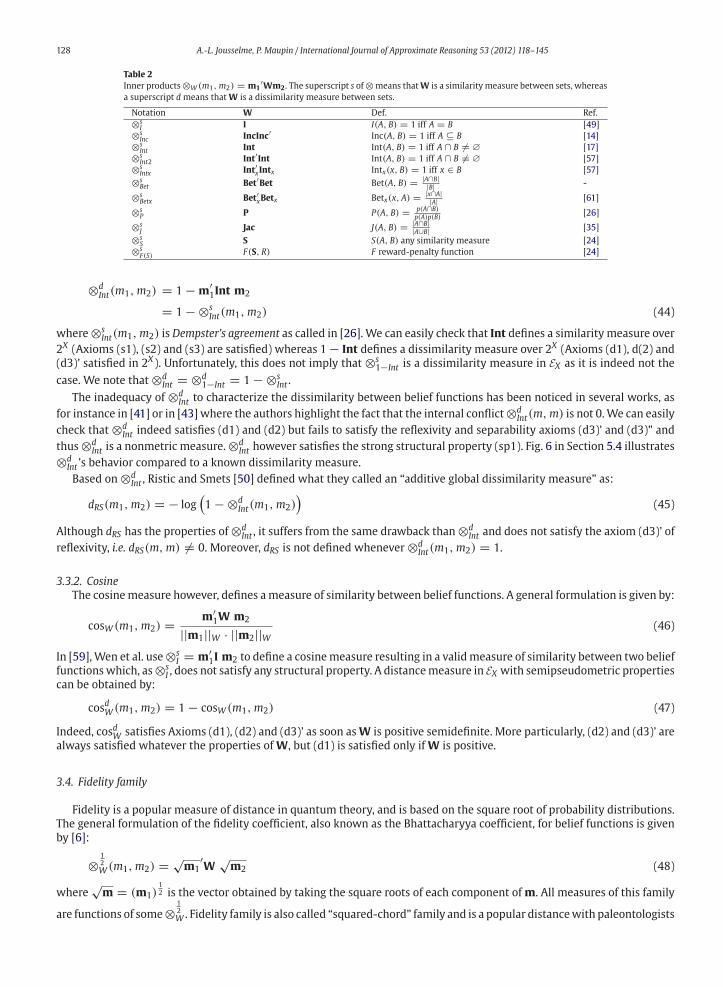
Table 2
Inner products⊗W (m1,m2) = m1′Wm2 . The superscript s of⊗means thatW is a similarity measure between sets, whereas
a superscript d means that W is a dissimilarity measure between sets.
Notation W Def. Ref.
⊗sI I I(A, B) = 1 iff A = B [49]
⊗sInc IncInc′ Inc(A, B) = 1 iff A ⊆ B [14]
⊗sInt Int Int(A, B) = 1 iff A ∩ B �= ∅ [17]
⊗sInt2 Int′Int Int(A, B) = 1 iff A ∩ B �= ∅ [57]
⊗sIntx Int′xIntx Intx(x, B) = 1 iff x ∈ B [57]
⊗sBet Bet′Bet Bet(A, B) = |A∩B|
|B| -
⊗sBetx Bet′xBetx Betx(x, A) = |x∩A|
|A| [61]
⊗sP P P(A, B) = p(A∩B)
p(A)p(B)[26]
⊗sJ Jac J(A, B) = |A∩B|
|A∪B| [35]
⊗sS S S(A, B) any similarity measure [24]
⊗sF(S) F(S, R) F reward-penalty function [24]
⊗dInt(m1,m2) = 1 − m′
1Int m2
= 1 − ⊗sInt(m1,m2) (44)
where⊗sInt(m1,m2) is Dempster’s agreement as called in [26]. We can easily check that Int defines a similarity measure over
2X (Axioms (s1), (s2) and (s3) are satisfied) whereas 1 − Int defines a dissimilarity measure over 2X (Axioms (d1), d(2) and
(d3)’ satisfied in 2X ). Unfortunately, this does not imply that ⊗s1−Int is a dissimilarity measure in EX as it is indeed not the
case. We note that ⊗dInt = ⊗d
1−Int = 1 − ⊗sInt .
The inadequacy of ⊗dInt to characterize the dissimilarity between belief functions has been noticed in several works, as
for instance in [41] or in [43] where the authors highlight the fact that the internal conflict⊗dInt(m,m) is not 0.We can easily
check that ⊗dInt indeed satisfies (d1) and (d2) but fails to satisfy the reflexivity and separability axioms (d3)’ and (d3)” and
thus⊗dInt is a nonmetric measure.⊗d
Int however satisfies the strong structural property (sp1). Fig. 6 in Section 5.4 illustrates
⊗dInt ’s behavior compared to a known dissimilarity measure.
Based on ⊗dInt , Ristic and Smets [50] defined what they called an “additive global dissimilarity measure” as:
dRS(m1,m2) = − log(1 − ⊗d
Int(m1,m2))
(45)
Although dRS has the properties of ⊗dInt , it suffers from the same drawback than ⊗d
Int and does not satisfy the axiom (d3)’ of
reflexivity, i.e. dRS(m,m) �= 0. Moreover, dRS is not defined whenever ⊗dInt(m1,m2) = 1.
3.3.2. Cosine
The cosinemeasure however, defines ameasure of similarity between belief functions. A general formulation is given by:
cosW (m1,m2) = m′1W m2
||m1||W · ||m2||W (46)
In [59],Wen et al. use⊗sI = m′
1I m2 to define a cosinemeasure resulting in a validmeasure of similarity between two belief
functionswhich, as⊗sI , does not satisfy any structural property. A distancemeasure in EX with semipseudometric properties
can be obtained by:
cosdW (m1,m2) = 1 − cosW (m1,m2) (47)
Indeed, cosdW satisfies Axioms (d1), (d2) and (d3)’ as soon asW is positive semidefinite. More particularly, (d2) and (d3)’ are
always satisfied whatever the properties of W, but (d1) is satisfied only if W is positive.
3.4. Fidelity family
Fidelity is a popular measure of distance in quantum theory, and is based on the square root of probability distributions.
The general formulation of the fidelity coefficient, also known as the Bhattacharyya coefficient, for belief functions is given
by [6]:
⊗12W (m1,m2) = √
m1′W
√m2 (48)
where√
m = (m1)12 is the vector obtained by taking the square roots of each component ofm. All measures of this family
are functions of some⊗12W . Fidelity family is also called “squared-chord” family and is a popular distancewith paleontologists
A.-L. Jousselme, P. Maupin / International Journal of Approximate Reasoning 53 (2012) 118–145 129
and in palynology studies. In probability theory, the Bhattacharyya (or fidelity) coefficient measures the amount of overlap
between two statistical populations.
It has been originally extended to belief functions by Ristic and Smets in [50] who proposed a Hellinger distance11 [33]
based on ⊗12W :
d(H)I (m1,m2) =
(1 − ⊗
12I (m1,m2)
) 12
(49)
A modified version of (49) has been proposed by Florea and Bossé in [27], obtained by replacing the square root by any
a-root, with a ∈ IR+∗. Based on I, this distance does not satisfy either (sp1) nor (sp2) but it is nevertheless a full metric
(Axioms (d1) to (d4) are satisfied).
3.5. Information-based distances
Besides the extension of the probabilistic form of themetric distance family, another quantification of the idea of distance
between two belief functions can be materialized by estimating the difference in their information content. As introduced
at the beginning of this section, the first attempt is due to Perry and Stephanou [46] who proposed an extension of Kullback–
Liebler divergence. But other works are worth mentioning.
In [20], in order to measure the quality of belief function approximations, Denœux proposed to quantify the distance
between m1 and m2 by the difference between the information contents of m1 and m2. The measure of uncertainty used
is the generalized cardinality of a belief function defined in [25] as GC(m) = ∑A⊆X m(A)|A| or using the matrix notation,
GC(m) = m′cA where cA is the column vector of cardinalities 12 of A (denoted as CardA in [53]). We have thus:
dGC(m1,m2) = |(m1 − m2)′cA| (50)
The general formulation was also mentioned in [20]:
dU(m1,m2) = |U(m1) − U(m2)| (51)
where U is any uncertainty measure defined for belief functions (see for instance [39] for a survey). Note that for the
practical use in [20] it was always true that GC(m1) ≥ GC(m2) and thus that dGC(m1,m2) ≥ 0. Although the original
measure did not explicitly include the absolute value we think it was implicit. And accordingly we have decided to add it
in the present definition insuring that the resulting distance satisfies the minimal property of nonnegativity (axiom (d1)).
Moreover, with the formulation (50) axioms (d2) and (d3)’ are satisfiedwhile axioms (d3)” and (d4) are not satisfied,making
dGC a semipseudometric.
Also, in [19], Denœux proposed that a cross-entropy measure dCE(m1,m2) = −m′1 log2(m2) + (1−m1)
′ log2(1−m2)
could be used as an alternative to the Euclidean distance d(2)ν for optimizing neural network weights.
3.6. Two-dimensional distances
In [41], Liu defined a two-dimensional measure to formally quantify the conflict between belief functions, as she noticed
that neither Dempster’s conflict alone, nor a distance alone is satisfactory. She then proposed the following index:
d2DL =(⊗d
Int(m1,m2); d(∞)Bet (m1,m2)
)(52)
She argues that “only when both measures are high, it is safe to say the evidence is in conflict” [41]. Indeed, ⊗dInt acts as the
anglemeasurewhile d(∞)Bet is themetricmeasure, the twomeasures being based on two different inner products (see Section
4.5). This principle can be extended to any other two inner products and the general formulation extending (52) is then:
d2D(W,V)(m1,m2) =(⊗d
W (m1,m2); dV (m1,m2))
(53)
It is not required for ⊗d and d to be defined upon the same inner product, hence one may be based on a weighting matrix
W while the other on a different matrix V, possibly increasing the complementarity of the two measures. As we will see in
Section 5.2, the correlation coefficient between measures may also be a criterion for building two-dimensional measures.
4. Outcomes
We provided four general formulations of distances between belief functions in Eqs. (20), (42), (47) and (48), which
encompassmost of the distances defined so far in the technical literature. Moreover, we provided a general formulation (53)
11 Up to a factor 2.12 Vector cA is closely linked to vector gA introduced in Section 3.1 and we have gA = cA−1
|X|−1.
130 A.-L. Jousselme, P. Maupin / International Journal of Approximate Reasoning 53 (2012) 118–145
Table 3
Distances between belief functions in their respective family (Lp , inner product or Fidelity), according to several definitions of the weighting matrix W. The
distances defined so far are in gray cells while new ones are in white cells.
Lp Inner product Fidelity
W = U′U p = 1 p = 2 p = ∞ IP cos (Hellinger)
I d(1)I d
(2)I d
(∞)I ⊗s
I cosI d(H)I
IncInc′ d(1)Inc d
(2)Inc d
(∞)Inc ⊗s
Inc cosInc d(H)Inc
Int d(1)Int d
(2)Int d
(∞)Int ⊗s
Int cosInt d(H)Int
Int′Int d(1)Int2 d
(2)Int2 d
(∞)Int2 ⊗s
Int2 cosInt2 d(H)Int
Int′xIntx d(1)Intx d
(2)Intx d
(∞)Intx ⊗s
Intx cosIntx d(H)Intx
Bet′Bet d(1)Bet d
(2)Bet d
(∞)Bet ⊗s
Bet cosBet d(H)Bet
Bet′xBetx d(1)Betx d
(2)Betx d
(∞)Betx ⊗s
Betx cosBetx d(H)Betx
P d(1)P d
(2)P d
(∞)P ⊗s
P cosP d(H)P
Jac d(1)J d
(2)J d
(∞)J ⊗s
J cosJ d(H)J
S d(1)S d
(2)S d
(∞)S ⊗s
S cosS d(H)S
F(S, R) d(1)F(S,R) d
(2)F(S,R) d
(∞)F(S,R) ⊗s
F(S,R) cosF(S,R) d(H)F(S,R)
Table 4
Axiomatic properties of the distances defined so far (see Table 1 and Section 2.5 for the axiom definitions).
for a two-dimensional measure. In this section we synthesize further our survey and sketch some ideas to be developed in
future research.
4.1. Summary and new measures
Table 3 summarizes the distances defined so far (gray cells) and provides the natural generalizations (white cells) hence
new distances.
Twenty-three distances have been defined so far and the generalization has led tomore than 40 newones. TheMinkowski
L2 family is the most numerous while L1 and L∞ have been seldom used. Extending the L2 distances to the study of L1 and
L∞ distances requires in some cases a Cholesky decomposition of the weighting matrices W. A single cosine measure has
been defined so far but a multitude of measures of this kind remains to be explored. This comment also applies to the
Hellinger distance and to other distances of the Fidelity family which are based on Bhattacharyya’s coefficient involving the
squared-root of the BPAs.
4.2. Metric and structural properties
Table 4 summarizes the algebraic properties of the distances together with their structural properties.
Distances with the highest number of metric properties appear at the top of the table while weakest metric distances
appear at the bottom. All distances are symmetric. Most of the distances are nonnegative. However, the two composite
measures dPS and dBP may have negative values due in both cases to their second member dPS(2) and dBP(2) respectively.
The second discrimination criterion between the distances is the definiteness property (d3) which splits into the reflexivity
property (d3)’ and the separability property (d3)”. The reflexivity means that d(m,m) = 0 and if not satisfied makes
the distances qualifying as nonmetric distances. In our case of study, distances not satisfying this property are all based on
A.-L. Jousselme, P. Maupin / International Journal of Approximate Reasoning 53 (2012) 118–145 131
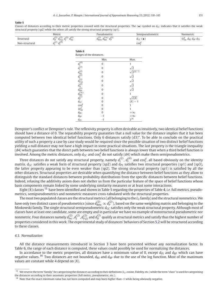
Table 5
Classes of distances according to their metric properties crossed with the structural properties. The (�) symbol on dGC indicates that it satisfies the weak
structural property (sp2) while the others all satisfy the strong structural property (sp1).
Metric Pseudometric Semipseudometric Nonmetric
Structural d(2)D d
(2)F(J) d
(2)J d
(2)Inc d
(2)Betx d
(∞)Bet d
(2)P dGC (�) ⊗d
Int dRS dBP dPS
Non-structural d(2)I d
(H)I cosdI
Table 6
Ranges of the distances.
Min. Max.
d(H)I 0 1
d(2)I 0
√2
d(2)Inc 0
√2|X|−1
d(2)J 0
√2
d(2)F(J) 0
√2
d(2)D 0
√2
d(2)Bet 0
√2
d(∞)Bet 0 1
d(2)P 0
√2|X|
dGC 0 |X| − 1
cosdI 0 1
⊗dInt 0 1
dRS 0 +∞dBP -1 +∞dPS -1 2|X|
Dempster’s conflict or Dempster’s rule. The reflexivity property is often desirable as intuitively, two identical belief functions
should have a distance of 0. The separability property guaranties that a null value for the distance implies that it has been
computed between two identical belief functions. Only 6 distances satisfy (d3)”. To be able to conclude on the practical
utility of such a property a case by case study would be required since the possible situation of two distinct belief functions
yielding a null distance may not have a high impact in some practical situations. The last property is the triangle inequality
(d4) which guaranties that the direct path between two belief functions is always lower than when a third belief function is
involved. Among the metric distances, only dGC and cosdI do not satisfy (d4) which make them semipseudometrics.
Three distances do not satisfy any structural property, namely d(2)I , d
(H)I and cosdI , all based obviously on the identity
matrix. dGC satisfies a weak form of structural property (sp2) and dPS satisfies two structural properties (sp1) and (sp3),
the latter property appearing to be even weaker than (sp2). The strong structural property (sp1) is satisfied by all the
other distances. Structural properties are desirable when quantifying the distance between belief functions as they allow to
distinguish the standard distances between probability distributions from the specific distances between belief functions.
Indeed, relaxing the additivity axiom does not shelter us from the particular feature of the space of belief functions whose
basis components remain linked by some underlying similarity measures or at least some interactions.
Eight (8) classes 13 have been identified and shown in Table 5 regarding the properties of Table 4, i.e. full metrics, pseudo-
metrics, semipseudometrics and nonmetric measures cross-tabulated with the structural properties.
Themost twopopulatedclassesare thestructuralmetrics (all belonging to the L2 family) and thestructuralnonmetrics.We
have only two distinct cases of pseudometrics (since d(2)Betx ∝ d
(2)P ), based on the sameweightingmatrix and belonging to the
Minkowski family. The single structural semipseudometric dGC satisfies only theweak structural property. Althoughmost of
classes have at least one candidate, some are empty and in particularwe have no example of nonstructural pseudometric nor
nonmetric. Four distances namely d(2)Inc , d
(2)J , d
(2)F(J) and d
(2)D qualify as structuralmetrics and satisfy thus the highest number of
properties considered in thiswork. The experimental study of distances’ behaviors of Section 5.2will be structured according
to these classes.
4.3. Normalization
All the distance measurements introduced in Section 3 have been presented without any normalization factor. In
Table 6, the range of each distance is computed, these values could possibly be used for normalizing the distances.
In accordance to the metric properties, all distances have a minimum value of 0, except dPS and dBP which can have
negative values. 14 Two distances are not bounded, dRS and dBP due to the use of the log function. Most of the maximum
values are constant while 4 depend on |X|.
13 We reserve the term“family” for categorizing thedistances according to their definitions (L2, cosine, Fidelity, etc.)while the term“class” is used for categorizing
the distances according to their axiomatic properties (full metric, pseudometric, etc.).14 Note that the exact minimum value has not been computed and may been higher than -1 while being obviously negative.
132 A.-L. Jousselme, P. Maupin / International Journal of Approximate Reasoning 53 (2012) 118–145
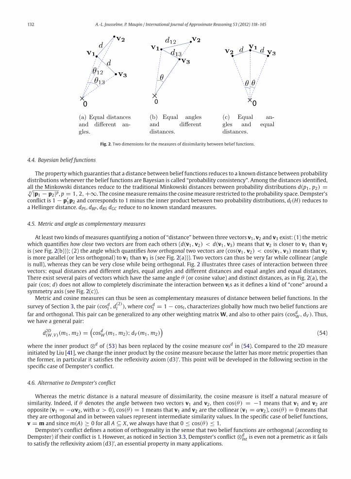
Fig. 2. Two dimensions for the measures of dissimilarity between belief functions.
4.4. Bayesian belief functions
The propertywhich guaranties that a distance between belief functions reduces to a known distance between probability
distributions whenever the belief functions are Bayesian is called “probability consistency”. Among the distances identified,
all the Minkowski distances reduce to the traditional Minkowski distances between probability distributions d(p1, p2) =p√|p1 − p2|p, p = 1, 2, +∞. The cosinemeasure remains the cosinemeasure restricted to the probability space. Dempster’s
conflict is 1 − p′1p2 and corresponds to 1 minus the inner product between two probability distributions, dI(H) reduces to
a Hellinger distance. dPS , dBP , dRS dGC reduce to no known standard measures.
4.5. Metric and angle as complementary measures
At least two kinds of measures quantifying a notion of “distance” between three vectors v1, v2 and v3 exist: (1) themetric
which quantifies how close two vectors are from each others (d(v1, v2) < d(v1, v3) means that v2 is closer to v1 than v3is (see Fig. 2(b))); (2) the angle which quantifies how orthogonal two vectors are (cos(v1, v2) < cos(v1, v3) means that v2is more parallel (or less orthogonal) to v1 than v3 is (see Fig. 2(a))). Two vectors can thus be very far while collinear (angle
is null), whereas they can be very close while being orthogonal. Fig. 2 illustrates three cases of interaction between three
vectors: equal distances and different angles, equal angles and different distances and equal angles and equal distances.
There exist several pairs of vectors which have the same angle θ (or cosine value) and distinct distances, as in Fig. 2(a), the
pair (cos; d) does not allow to completely discriminate the interaction between vis as it defines a kind of “cone” around a
symmetry axis (see Fig. 2(c)).
Metric and cosine measures can thus be seen as complementary measures of distance between belief functions. In the
survey of Section 3, the pair (cosdI , d(2)I ), where cosdI = 1 − cosI , characterizes globally how much two belief functions are
far and orthogonal. This pair can be generalized to any other weighting matrix W, and also to other pairs (cosdW , dV ). Thus,we have a general pair:
d2D(W,V)(m1,m2) =(cosdW (m1,m2); dV (m1,m2)
)(54)
where the inner product ⊗d of (53) has been replaced by the cosine measure cosd in (54). Compared to the 2D measure
initiated by Liu [41], we change the inner product by the cosine measure because the latter has more metric properties than
the former, in particular it satisfies the reflexivity axiom (d3)’. This point will be developed in the following section in the
specific case of Dempster’s conflict.
4.6. Alternative to Dempster’s conflict
Whereas the metric distance is a natural measure of dissimilarity, the cosine measure is itself a natural measure of
similarity. Indeed, if θ denotes the angle between two vectors v1 and v2, then cos(θ) = −1 means that v1 and v2 are
opposite (v1 = −αv2, with α > 0), cos(θ) = 1 means that v1 and v2 are the collinear (v1 = αv2), cos(θ) = 0 means that
they are orthogonal and in between values represent intermediate similarity values. In the specific case of belief functions,
v = m and since m(A) ≥ 0 for all A ⊆ X , we always have that 0 ≤ cos(θ) ≤ 1.
Dempster’s conflict defines a notion of orthogonality in the sense that two belief functions are orthogonal (according to
Dempster) if their conflict is 1. However, as noticed in Section 3.3, Dempster’s conflict ⊗dInt is even not a premetric as it fails
to satisfy the reflexivity axiom (d3)’, an essential property in many applications.
A.-L. Jousselme, P. Maupin / International Journal of Approximate Reasoning 53 (2012) 118–145 133
In order to maintain the notion of conflict that it defines while having the properties of a semipseudometric, one could
think of the following cosine-based measure:
cosdInt(m1,m2) = 1 − m′1Intm2
‖m1‖Int · ‖m2‖Int
(55)
= 1 − ⊗sInt(m1,m2)√
⊗sInt(m1,m1).
√⊗s
Int(m2,m2)(56)
where ‖ · ‖Int denotes the norm relatively to the matrix Int and ⊗sInt is Dempster’s agreement. Indeed, normalizing the
inner product by both the norm of m1 and m2 guaranties that cosdInt(m,m) = 0, axiom (d3)’ of reflexivity is satisfied.
Unfortunately, because Int is nonpositive, cosdInt is not positive. So we gained one interesting property but we lost another
one, the nonnegativity (d1).
The alternative matrix Int Int however is positive definite and could thus be used as a basis for an alternative measure
to Dempster’s conflict:
cosdInt2(m1,m2) = 1 − m′1Int Intm2
‖m1‖Int2.‖m2‖Int2
(57)
= 1 − Pl′1Pl2‖Pl1‖.‖Pl2‖ (58)
where we noticed that Int is symmetric and Pl = Int m. Now the three basic axioms of a semipseudometric measure (d1),
(d2) and (d3)’ are satisfied. But remains the question of the meaning of IntInt. Indeed, the elements of IntInt are:
Int2(A, B) = |{A ∩ C} ∩ {B ∩ C}|, ∀C ⊆ X (59)
that is the number of subsets C ⊆ X intersecting with both A and B. cossInt2 quantifies thus a “second-order” notion of
agreement since Int2 quantifies how much two given subsets intersect through the mediation of a third one. The “first-
order” agreement (Dempster’s) only quantifies if or if not two given subsets intersect directly with each other. Theminimum
agreement between two subsets A and B according to Int2(A, B) is 2N−2 and is reached when A ∩ B = ∅ and A and B are
singletons. If A∩ B = ∅ and A and B are not singletons, then Int2 is thus higher and depends on the cardinalities of A and B.
The maximum of Int2(A, B) is Int2(X, X) = 2N − 1. Thus, two belief functions without focal elements in interaction, which
would mean a null agreement according to ⊗sInt may exhibit a nonnull agreement according to cossInt2.
The associated Euclidean distance in the inner product space with Int Int as weighting matrix is:
d(2)Int2(m1,m2) =
√(m1 − m2)′Int′Int(m1 − m2) (60)
= ‖Pl1 − Pl2‖ (61)
= ‖Bel1 − Bel2‖ (62)
= d(2)Inc (63)
Thus, the standard Euclidean distance between belief functionswould be the associatedmetric to ameasure of angle derived
from a “second-order” Dempster’s conflict. This is due to the duality of Pl and Bel in the closed world. Nonetheless, the two
weighting matrices Int Int and Inc Inc′ are different and thus cosdInt2 �= cosdInc and they measure two distinct kinds of
angles.
4.7. Encoding of belief functions
The four well known functions of basic probability assignment, belief, plausibility and commonality are four different
encodings of the same information. Defining Euclidean distances between two functions of the same kind leads to different
distances when referring to a representation of reference that is a BPA, hence different values for the same two objects. For
instance, we saw that d(2)I (the Euclidean distance between BPAs) is different from d
(2)Inc (the Euclidean distance between
belief functions). Also we have d(2)Inc = d
(2)Int2 due to the duality between Pl and Bel under the closed world assumption. But
d(2)Inc′ , the Euclidean distance between two commonality functions built upon the weighting matrix Inc′Inc is different from
the three others and would be worth to be considered in future works.
Besides these well known encodings of belief functions other encodings can be defined with however less obvious
interpretations. For instance, we may define:
fJ = UJm (64)
where UJ is the upper triangle matrix resulting from the Cholesky decomposition of the Jaccard matrix Jac. Or expressed
under the form of Eq. (10):
134 A.-L. Jousselme, P. Maupin / International Journal of Approximate Reasoning 53 (2012) 118–145
fJ(A) = ∑B⊆X
m(B)UJ(A, B) (65)
where UJ(A, B) is the element (A, B) of matrixUJ . Equivalently, we could define fD, fP , etc, corresponding respectively to Dice
matrix, BPAM matrix.
The interest of considering the basic encoding for belief functions (i.e. the BPA) lies in the fact that it highlights the
strong structural property of the weighted Euclidean distance. However, we could define some combinations such as for
instance BelJ defined such that BelJ = UJBel = UJ Inc′m. Then the Euclidean distance between Bel1J and Bel2J would be
defined as:
d(2)I (Bel1J , Bel
2J ) = d
(2)IncJ(m1,m2)
=√
(Bel1J − Bel2J )′(Bel1J − Bel2J )
=√
[UJ Inc′(m1 − m2)]′UJ Inc
′(m1 − m2)
=√
(m1 − m2)′Inc Jac Inc′(m1 − m2) (66)
Such formulations would reinforce the impact of the similarity between the basis vectors of EX .
4.8. Generalizations
1. Fuzzy belief functions:
The above measures can be further generalized to fuzzy belief functions by making the weights W(A, B) be
measures of similarity between fuzzy sets. As an example, in [47] Petit-Renaud and Denœux defined an error
criterion for fuzzy belief structures based on ⊗dPR(m1,m2) = m′
1DPRm2 where DPR is the matrix composed of
elements dPR(A, B) which itself is a distance between fuzzy sets A and B.
2. Open world assumption:
We restricted the studyof thedistances to the closedworld assumption (or normality assumption, i.e.m(∅) = 0).
Although the extension to the open world assumption would require a deeper analysis, a preliminary analysis
showed that most of the distances presented keep all their properties for BPAs with a non-null mass to the empty
set,whileothersdegenerate frommetrics topseudometrics. The latter are Lp distances involvingweightingmatrices
whichbecomenondefinitewhen thedimensione∅ is added (d(p)J ,d
(p)F(J),d
(p)D ). It seems thatd
(p)Inc keeps its definiteness
property.
5. Experimental comparison
5.1. Toy example
We illustrate the behavior of the different classes of distances of Table 5 on the toy example introduced in [35] and reused
in [41]. Let X = {x1, . . . , x10} be a frame of discernment and let Belt be a belief function defined over X such that
At is a variable focal element ranging from {x1} to X , one element xi being added at each step. Let Bel∗ be a categorical
belief function representing a targeted belief function (e.g. representing the ground truth in a given problem) and defined
by
Bel∗ = ({x1, x2, x3, x4, x5}, 1) (68)
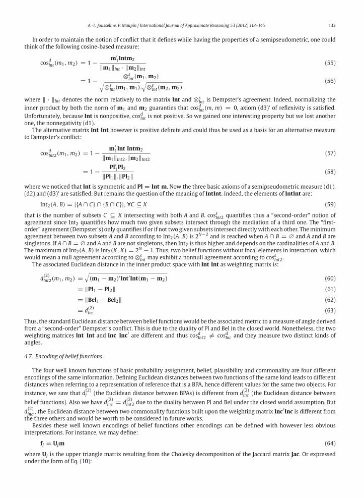
The three graphics in Fig. 3 show the behaviors of the distances identified in Section 3 assembled into the several families
identified in Table 5, i.e. (full) metrics in the first graphic, pseudometrics and semipseudometrics in the second graphic, and
nonmetrics in the third graphic. Nonstructural distances are represented with dashed lines. In each of the three graphics,
distances of a variable belief function Belt (one focal element At only is variable) to a categorical belief function Bel∗ of the
form m∗({x1, x2, x3, x4, x5}) = 1 are shown, with At varying from {x1} to {x1, . . . , x10}. For the simulations, all distances
have been normalized with the range values of Table 6.
For themetrics classofdistances (first graphic),weobservesimilarbehaviors forall the structuraldistanceswhiledenoting
however a small difference for the d(2)Inc distance. The two nonstructural distances behave similarly while differently from
the structural ones, as they unsurprisingly remain constant when At varies and only decrease when At reaches A∗ at time
step 5. We also note a slight increase of d(2)I at the last time step when At reaches X since the number of focal elements for
Belt has changed from 4 to 3.
A.-L. Jousselme, P. Maupin / International Journal of Approximate Reasoning 53 (2012) 118–145 135
Fig. 3. Distances of a variable belief function Belt (i.e. At varies from {x1} to {x1, . . . , x10}) to a categorical belief function Bel∗ , i.e. m∗({x1, x2, x3, x4, x5}) = 1.
Nonstructural distances are represented with dashed lines.
The secondgraphic shows thebehaviors of thepseudometrics and the semipseudometrics together. Only 3pseudometrics
are visible since d(2)Betx ∝ d
(2)P and because the distances have been normalized, d
(2)P and d
(2)Betx are confounded. The two
pseudometrics of type dBet (and of course d(2)P ) behave similarly. The two semipseudometrics have distinct behaviors: dGC
increases linearly with the number of elements in At , while the nonstructural cosine measure remains constant while At
varies and reaches a minimum at time step 5 where At reaches A∗.
Thenonmetricmeasures are shown in the thirdgraphic. The twobelief functions consideredyield toa constantDempster’s
conflict, ⊗dInt(mt,m
∗) = mt({x7})m∗({x1, x2, x3, x4, x5}) = 0.05, and consequently dRS and dBP remain also very low since
they are based on ⊗dInt . We observe however a slight increase of dBP due to its second member dBP(2). The behavior of dPS is
similar to other nonstructural distances while we note a decrease at the last time step when At = X . Indeed, dPS(1), the first
136 A.-L. Jousselme, P. Maupin / International Journal of Approximate Reasoning 53 (2012) 118–145
member of dPS , remains constant and equal to 5 except when At reaches A∗ where it is 3. The secondmember dPS(2) remains
negative15 .
In the light of the example above, it appears that the structural properties (sp1) and (sp2) strongly influence the behavior
of the different distances. Moreover, the structural dissimilarity (sp3) (only satisfied by dPS) is not sensitive to this example
of convergence toward a categorical belief function, and makes this “structural distance” close to nonstructural ones. The
accounting of the focal elements interaction defined by (sp3) (i.e. the interaction of sets of focal elements) is thus too rough
compared to (sp1) and (sp2). Also, we do not denote any significant behavior difference betweenmetrics and pseudometrics
while distances involving Dempster’s conflict behave similarly.
5.2. Semantic comparison
The results discussed in this part give only a hint of what a deeper study of this kind would bring. Rather than drawing
specific and complete conclusions, themain aim of this experimental section is to highlight some properties of the distances
that would be worth considering when selecting a distance for a particular practical purpose.
We follow the techniquedescribed in [11] for analyzing the semantic similarities betweendissimilaritymeasuresbetween
belief functions. Ns belief functions are randomly generated {Beln}Ns
n=1 (as described by Algorithm 1).
Input: X: Frame of discernment
Output: Bel: Belief function (under the form of a BPA, m)
Generate the power set of X → 2X ;
Generate a random permutation of 2X → R(X);Generate a integer between 1 and Nmax → k;
foreach First randomly generated k elements of R(X) doGenerate a value within [0, 1] → mk;
end
Normalize the vector m = [m1 . . .mk] → m∗;m(Ak) = mk;
Algorithm 1: Random generation of a belief function.
We have generated five different types of BPAs: (1) simple support, i.e. m(A) = α, m(X) = 1 − α,(2) dichotomous, i.e.
m(A) = α, m(A) = β , m(X) = 1 − α − β , (3) complete, i.e. with 2|X| − 1 focal elements (4) with a fixed number of focal
elements and (5) consonant, i.e.with nested focal elements. These types of BPAs have been used in the following to compare
some behaviors of the distances in specific experiments.
The distances previously introduced in Section 3 and gathered in a set D are then computed for each of the Ns pairs
(mr,mn), where mr is a unique belief function of reference also randomly generated. Note that because the algorithms for
random BPAs generation all involve a controlled number of focal elements (either 2, 3, 5 or 2|X| − 1) and that the masses are
then uniformly assigned, the impact of the BPA of reference on the result provided in the following is very low.
The resultspresented in this sectionhavebeenobtained for framesofdiscernmentwhosecardinality |X| ranges from2to8,
for anumberof replicationsNs between1000and10000dependingon theexperiment, and for a set of distancesof cardinality
|D| = 15. In d(2)P , the prior probability distribution has been assumed to be uniform over X so that P(A, B) = N|A∩B|
|A|.|B| . In d(2)F(J),
F has been chosen as in [24]. Although in the original paper [46], for the function dPS , the authors restricted the mis to be
simple support belief functions, we removed this restriction in our simulations.
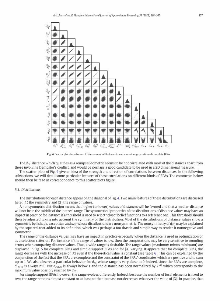
Fig. 4 shows the scatter plots for each pair(di(m
r,mn), dj(mr,mn)
), di, dj ∈ D for a cardinality of X of 8. The boxes
on the diagonal of the scatter plot show the distributions of the measures. A straight line in the scatter plots means strong
correlation (as for instance between dRS and⊗dInt , in accordance to their respective definitions)while a cloud of pointsmeans
a weak correlation (as for instance between ⊗dInt and d
(∞)Bet ).
Due to the ordering of the distances according to their axiomatic properties, the correlation of the metrics and pseudo-
metrics appear on the top of the figure. We observe a strong correlation between all the structural distances of the Lp family
metrics and pseudometrics. No clear conclusion can be drawn whether the correlation is due to the family (Lp) or to the
class (metric versus pseudometric), since we do not have enough examples of each class. We can simply notice a stronger
correlation between the three nonstructural metrics whose weighting matrix are known similarity measures between the
focal sets, say d(2)J , d
(2)F(J) and d
(2)D than with the nonstructural metric d
(2)Inc .
The distances involving Dempster’s conflict (and the conflict itself) ⊗dInt , dRS , dPS and dBP are not correlated with the
metric and pseudometric distances. Note that in this particular case of complete BPAs, the first member of the distance dPSis always 0 and thus we only observe the second member dPS(2) in the scatter plots. For other kinds of BPAs, we would have
observed steps corresponding to the integer values dPS(1).
15 Note that here the values have been normalized relatively to |F1 ∩ F2| + 1 which is the maximum value in this example, and not to 2|X| so that the values
are not too close to 0.
A.-L. Jousselme, P. Maupin / International Journal of Approximate Reasoning 53 (2012) 118–145 137
Fig. 4. Scatter plots for a frame of discernment of 8 elements and a random generation of complete BPAs.
The dGC distancewhich qualifies as a semipseudometric seems to be noncorrelatedwithmost of the distances apart from
those involving Dempster’s conflict, and would be perhaps a good candidate to be used in a 2D dimensional measure.
The scatter plots of Fig. 4 give an idea of the strength and direction of correlations between distances. In the following
subsections, we will detail some particular features of these correlations on different kinds of BPAs. The comments below
should then be read in correspondence to this scatter plots figure.
5.3. Distributions
The distributions for each distance appear on the diagonal of Fig. 4. Twomain features of these distributions are discussed
here: (1) the symmetry and (2) the range of values.
A nonsymmetric distributionmeans that higher (or lower) values of distances will be favored and that amedian distance
will not be in themiddle of the interval range. The symmetrical properties of the distributions of distance valuesmay have an
impact in practice for instance if a threshold is used to select “close” belief functions to a reference one. This threshold should
then be adjusted taking into account the symmetry of the distribution. Most of the distributions of distance values show a
symmetric bell shape, except dBP and dGC whose distributions are nonsymmetric. The nonsymmetry of dGC may be explained
by the squared-root added to its definition, which was perhaps a too drastic and simple way to render it nonnegative and
symmetric.
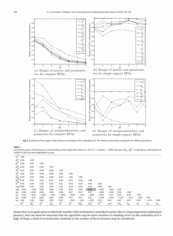
The range of the distance values may have an impact in practice especially when the distance is used in optimization or
as a selection criterion. For instance, if the range of values is low, then the computations may be very sensitive to rounding
errors when comparing distance values. Thus, a wide range is desirable. The range values (maximumminus minimum) are
displayed in Fig. 5 for complete BPAs and simple support BPAs and for |X| varying. It appears that for complete BPAs, the
range decreases with the increase of |X| even if the theoretical value is constant (see Table 6). This can be explained by the
conjunction of the fact that the BPAs are complete and the constraint of the BPAs’ coordinates which are positive and to sum
up to 1. We also observe a particular behavior for dPS whose range is very close to 0. Indeed, since the BPAs are complete,
dPS(1) is always null. But dPS(2) is always below 1 and the distance has been normalized by 2|X| which corresponds to the
maximum value possibly reached by dPS .
For simple support BPAs however, the range evolves differently. Indeed, because the number of focal elements is fixed to
two, the range remains almost constant or at least neither increase nor decreases whatever the value of |X|. In practice, that
138 A.-L. Jousselme, P. Maupin / International Journal of Approximate Reasoning 53 (2012) 118–145
Fig. 5. Evolution of the ranges of the distances according to the cardinality of X . The statistics have been computed over 10000 replications.
Table 7
Correlation matrix of the distances corresponding to the scatter plot of Fig. 4, i.e. for |X| = 8 and Ns = 6000. The pair (⊗dInt , d
means that in an application inwhich thenumber of focal elements is intended to grow (like in a long sequential combination
process), then we must be conscious that the algorithm may be more sensitive to rounding errors as the cardinality of X is
high. Perhaps, a kind of normalization relatively to the number of focal elements may be considered.
A.-L. Jousselme, P. Maupin / International Journal of Approximate Reasoning 53 (2012) 118–145 139
2 3 4 5 6 7 8−0.8
−0.6
−0.4
−0.2
0
0.2
0.4
0.6
0.8
1
|X|
Cor
rela
tion
coef
fici
ents
c(dJ(2);d
I(2))
c(dJ(2);d
Inc(2))
c(dJ(2);d
GC)
c(dJ(2);d
Bet∞ )
c(dJ(2);d
I(H))
c(dJ(2);cos
Id)
c(dJ(2);⊗
Intd )
c(dJ(2);d
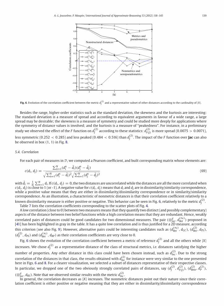
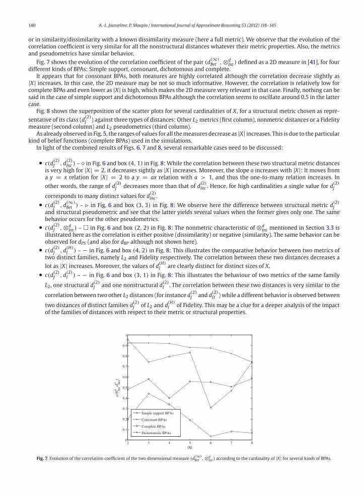
PS)
c(dJ(2);d
BP)
Nonstructural distances
Metrics and pseudometrics
Nonmetrics and semipseudometrics
Fig. 6. Evolution of the correlation coefficient between the metric d(2)J and a representative subset of other distances according to the cardinality of |X|.
Besides the range, higher-order statistics such as the standard deviation, the skewness and the kurtosis are interesting:
The standard deviation is a measure of spread and according to equivalent arguments in favour of a wide range, a large
spread may be desirable; the skewness is a measure of symmetry and could be studied more deeply for applications where
the symmetry of distance values is involved; and the kurtosis is a measure of “peakedness”. For instance, in a preliminary
study we observed the effect of the F function on d(2)J according to these statistics: d
(2)F(J) is more spread (0.0075 > 0.0071),
less symmetric (0.252 < 0.285) and less peaked (0.484 < 0.516) than d(2)J . The impact of the F function over Jac can also
be observed in box (1, 1) in Fig. 8.
5.4. Correlation
For each pair of measures in D, we computed a Pearson coefficient, and built corresponding matrix whose elements are:
c(di, dj) =∑N
n=1(dni − di)(d
nj − dj)√∑N
n=1(dni − di)2
√∑Nn=1(d
nj − dj)2
(69)
with di = 1N
∑Nn=1 di. If c(di, dj) = 0, the twodistances areuncorrelatedwhile thedistances are all themore correlatedwhen
c(di, dj) is close to 1 (or -1). A negative value for c(di, dj)means that di and dj are in dissimilarity/similarity correspondence,
while a positive value means that they are either in dissimilarity/dissimilarity correspondence or in similarity/similarity
correspondence. As an illustration, a characteristic of nonmetric distances is that their correlation coefficient relatively to a
known dissimilarity measure is either positive or negative. This behavior can be seen in Fig. 6, relatively to the metric d(2)J .
Table 7 lists the correlation coefficients corresponding to the scatter plots of Fig. 4.
A low correlation (close to 0) between twomeasuresmeans that they quantify twodistinct (and possibly complementary)
aspects of the distance between two belief functions while a high correlationmeans that they are redundant. Hence, weakly
correlated pairs of distances could be good candidates for two dimensional measures. The pair (⊗dInt, d
(∞)Bet ) proposed in
[41] has been highlighted in gray in the table. It has a quite low correlation and is thus justified for a 2D measure, according
this criterion (see also Fig. 9). However, alternative pairs could be interesting candidates such as (d(∞)Bet , dGC), (d
(2)Bet , dPS),
(d(2)P , dPS) and (d
(∞)Bet , dBP) as their correlation coefficients are very close to 0.
Fig. 6 shows the evolution of the correlation coefficient between a metric of reference d(2)J and all the others while |X|
increases. We chose d(2)J as a representative distance of the class of structural metrics, i.e. distances satisfying the higher
number of properties. Any other distance in this class could have been chosen instead, such as d(2)Inc . Due to the strong
correlation of the distances in that class, the results obtained with d(2)Inc for instance were very similar to the one presented
here in Figs. 6 and 8. For a clearer visualization, we selected a subset of distances representative of their respective classes.
In particular, we dropped one of the two obviously strongly correlated pairs of distances, say (d(2)J , d
(2)F(J)), (d
(2)Betx, d
(2)P ),
(⊗dInt, dRS). Note that we observed similar results with the metric d
(2)Inc .
In general, the correlation decreases as |X| increases. The nonmetric distances point out their nature since their corre-
lation coefficient is either positive or negative meaning that they are either in dissimilarity/dissimilarity correspondence
140 A.-L. Jousselme, P. Maupin / International Journal of Approximate Reasoning 53 (2012) 118–145
or in similarity/dissimilarity with a known dissimilarity measure (here a full metric). We observe that the evolution of the
correlation coefficient is very similar for all the nonstructural distances whatever their metric properties. Also, the metrics
and pseudometrics have similar behavior.
Fig. 7 shows the evolution of the correlation coefficient of the pair (d(∞)Bet , ⊗d
Int) defined as a 2D measure in [41], for four
different kinds of BPAs: Simple support, consonant, dichotomous and complete.
It appears that for consonant BPAs, both measures are highly correlated although the correlation decrease slightly as
|X| increases. In this case, the 2D measure may be not so much informative. However, the correlation is relatively low for
complete BPAs and even lower as |X| is high, which makes the 2Dmeasure very relevant in that case. Finally, nothing can be
said in the case of simple support and dichotomous BPAs although the correlation seems to oscillate around 0.5 in the latter
case.
Fig. 8 shows the superposition of the scatter plots for several cardinalities of X , for a structural metric chosen as repre-
sentative of its class (d(2)J ) against three types of distances: Other L2 metrics (first column), nonmetric distances or a Fidelity
measure (second column) and L2 pseudometrics (third column).
As already observed in Fig. 5, the ranges of values for all themeasures decrease as |X| increases. This is due to theparticularkind of belief functions (complete BPAs) used in the simulations.
In light of the combined results of Figs. 6, 7 and 8, several remarkable cases need to be discussed:
• c(d(2)J , d
(2)Inc ) – � in Fig. 6 and box (4, 1) in Fig. 8: While the correlation between these two structural metric distances
is very high for |X| = 2, it decreases sightly as |X| increases. Moreover, the slope a increases with |X|: It moves from
a y = x relation for |X| = 2 to a y = ax relation with a > 1, and thus the one-to-many relation increases. In
other words, the range of d(2)J decreases more than that of d
(2)Inc . Hence, for high cardinalities a single value for d
(2)J
corresponds to many distinct values for d(2)Inc .
• c(d(2)J , d
(∞)Bet ) – � in Fig. 6 and box (3, 3) in Fig. 8: We observe here the difference between structural metric d
(2)J
and structural pseudometric and see that the latter yields several values when the former gives only one. The same
behavior occurs for the other pseudometrics.
• c(d(2)J , ⊗d
Int) – � in Fig. 6 and box (2, 2) in Fig. 8: The nonmetric characteristic of ⊗dInt mentioned in Section 3.3 is
illustrated here as the correlation is either positive (dissimilarity) or negative (similarity). The same behavior can be
observed for dPS (and also for dBP although not shown here).
• c(d(2)J , d
(H)I ) – − in Fig. 6 and box (4, 2) in Fig. 8: This illustrates the comparative behavior between two metrics of
two distinct families, namely L2 and Fidelity respectively. The correlation between these two distances decreases a
lot as |X| increases. Moreover, the values of d(H)I are clearly distinct for distinct sizes of X .
• c(d(2)J , d
(2)I ) – − in Fig. 6 and box (3, 1) in Fig. 8: This illustrates the behaviour of two metrics of the same family
L2, one structural d(2)J and one nonstructural d
(2)I . The correlation between these two distances is very similar to the
correlation between two other L2 distances (for instance d(2)J and d
(2)D ) while a different behavior is observed between
two distances of distinct families d(2)J of L2 and d
(H)I of Fidelity. This may be a clue for a deeper analysis of the impact
of the families of distances with respect to their metric or structural properties.
Fig. 7. Evolution of the correlation coefficient of the two dimensional measure (d(∞)Bet , ⊗d
Int) according to the cardinality of |X| for several kinds of BPAs.
A.-L. Jousselme, P. Maupin / International Journal of Approximate Reasoning 53 (2012) 118–145 141
Fig. 8. Superposition of the scatter plots for several cardinalities ofX (from2 to 7)with 1000 replications of complete BPAs. Three groups of distances are compared
to a structural metric chosen as reference, d(2)J .
Fig. 9. Superposition of the scatter plots for several cardinalities of X (from 2 to 7) between four distances: Two pseudometrics of the same family, one similarity
measure and Dempster’s conflict.
Fig. 9 shows the scatter plots between several classes of measures: Two pseudometrics belonging to the same family Lp,
d(∞)Bet (L∞) and d
(2)Betx (L2), Dempster’s conflict⊗d
Int and the similaritymeasure cossI = 1−cosdI . We first observe that although
the two pseudometrics are based on the same weighting matrix Bet′Bet, these behave differently when compared to the
two other distances. This highlights the impact of the p coefficient within the Lp family. Maybe the latter could be the subject
of further investigations.
142 A.-L. Jousselme, P. Maupin / International Journal of Approximate Reasoning 53 (2012) 118–145
The correlation c(d(2)Bet , cos
sI ) is remarkable as it remains high whatever the cardinality of X while it is very distinct from
one cardinality to another.
The couple (d(∞)Bet , ⊗d
Int) corresponds to Liu’s 2D index and should be completed by the curve with diamonds in Fig. 7
corresponding to complete BPAs. In both graphics, we see that the correlation remains very low as |X| increases. However, we
also observe that the space in the scatter plot is only half-covered (upper-right triangle) meaning that a kind of correlation
exists between these two measures. The Pearson coefficient is only one measure of similarity among others, and behaviors
such as this one suggest studying other measures of similarity between distances.
5.5. Additive trees
Based on the correlation coefficient values, we built the additive trees (dendrograms) for all six cardinalities of X (Fig. 10).
The dendrograms are built using the correlation coefficient given by Eq. (69) as a similarity measure. For the construction
and interpretation of the trees the method presented in Sattath and Tversky’s classical paper [51] is used. The dissimilarity
Fig. 10. Additive trees computed on a Pearson correlation matrix between 10000 replications based on Algorithm 1 generating complete BPAs over a frame of
discernment whose cardinality varies from 2 to 8.
A.-L. Jousselme, P. Maupin / International Journal of Approximate Reasoning 53 (2012) 118–145 143
of two objects represented on these additive trees is simply given by the length of the path joining them, the longer the path,
the more dissimilar are the objects under study.
Referring to the classes identified in Table 5, four groups of distances are considered:Nonmetrics (red circles), pseudomet-
rics (green circles), metrics (blue circles) and nonstructural distances (yellow circles). These four groups clearly appear in the
trees although the tree structure is slightly sensitive to the size of the frame of discernment. Rather than the family (Lp, inner
product or Fidelity) it appears that the axiomatic properties play a major role in the similarity of the distances. Moreover,
the nonstructural property seems even stronger than the metric properties since the three nonstructural distances remain
clearly regrouped as |X| varies while one is a dissimilarity (cosdI ), one is a L2 metric (d(2)I ) and one is a Fidelity metric (d
(H)I ).
Metrics and pseudometrics are very close to each other and form two very compact groups. Nonmetric distances are not
so well assembled in a compact group but seem to behave very differently from the others. This is very clear for dPS while
dGC is sometimes closer to the other kinds of distances. We must outline that the nonmetric distances have another feature
in common apart from their nonmetric properties, which is that they all involve Dempster’s conflict. A deeper analysis
including other nonmetric measures not based on⊗dInt or metric measures based on⊗d
Int would be required to discriminate
the influence of ⊗dInt relatively to the metric properties.
The results of the experimentations presented here are not exhaustive and a lot of work remains to be done. However,
these preliminary results highlighted some remarkable experimentally observed features that we have been able to relate
to the theoretical properties. In practice, these results suggest that the choice of a measure should be guided by (1) the
structural properties, a structural distance being in general more desirable for the quantification of the distance between
two belief functions, (2) the metric properties since the definiteness may be also desirable in some cases. Regardless these
“technical” properties, semantic properties would also be worth some consideration as the meaning of the distance may be
of prime importance in some applications. For instance, dGC quantifies a difference in information contents which is very
different from d(p)Bet which quantifies the difference in decision abilities. It is not clear however how important is the family
the distances belong to, although we have been able to notice some impact of the p coefficient in the Lp family for instance.
6. Conclusions and future work
In this paper we have presented, together with a synthesis of their most important properties, a survey of the main
dissimilarity measures defined so far using the mathematical framework of evidence theory. The principal results of this
study are briefly recapitulated here, followed by a short discussion on future work.
We have first outlined the existence of a formal link between the existing distances defined so far in the mathematical
framework of belief functions and the theory of inner products. This helped us propose a grouping of the dissimilarity
measures into five families, i.e. Composite, Minkowski, Inner product, Fidelity and Information-based, families for which
we have provided general formulations. Building upon these generalizations we have subsequently defined more than 40
new distances. Then, we have proposed a classification based on the one hand (a) on the study of the metric properties of
the surveyed distance measurements allowing us to distinguish four groups (metrics, pseudometrics, semipseudometrics
and nonmetric measures) and on the other hand (b) on structural properties allowing us the distinguish two groups of
measurements (structural and nonstructural). This classification has been used later in the paper to interpret the results of
simulations aimed at the experimental comparison of the surveyed distance measurements.
We have also provided a general expression for two-dimensional indexes expressed as couples composed of a cosine
and a dissimilarity and proposed an alternative formulation to Dempster’s conflict based on a cosine measure. Using a toy
example about the monitoring of the convergence to a categorical belief function, we have illustrated the behavior of the
different families of distance measurements.
Experimental comparisonsbasedon the simulationof randomly assignedbeliefmasses for different frameof discernment
cardinalities allowed us to highlight the practical effects of the theoretical properties outlined in the present work, in
particular (a) that of the non metric property of Dempster’s conflict, as well as (b) the high correlation of measurements
obtainedwithin thesame formal family.Wehave thusbeenable to relateexperimentalobservations to someof the theoretical
properties of the measures studied, admittedly an unexpected finding for the authors.
This paper can be seen as a first attempt to synthesize the theoretical properties of the existing distancemeasurements in
themathematical framework of evidence theory.Muchwork remains to be done, either on the theoretical or on the practical
front of this emerging specialty. In future work we will refine the theoretical underpinnings outlined here, and pursue the
study of the new distance measurements discovered in the present study.
An important endeavor is to develop practical applications using the newly discovered measurements and to study their
behavior under different contexts of use. In the short term, future experimental work will include the development and
comparison of clustering and information retrieval methods.
Acknowledgments
We gratefully thank Dr. Mihai Florea for many useful discussions and for his support for some of the programming. We
would also like to thank the anonymous reviewers for their relevant and constructive comments which have helped us
improve the paper considerably.
144 A.-L. Jousselme, P. Maupin / International Journal of Approximate Reasoning 53 (2012) 118–145
References
[1] J. Abellán, M. Gómez, Measures of divergence on credal sets, Fuzzy Sets and Systems 157 (2006) 1514–1531.[2] M. Basseville, Distance measures for signal processing and pattern recognition, European Journal Signal Processing 18 (1989) 349–369.
[3] M. Bauer, Approximation algorithms and decisionmaking in the Dempster–Shafer theory of evidence – an empirical study, International Journal of Approx-imate Reasoning 17 (1997) 217–237.
[4] S. Ben-Hariz, Z. Elouedi, K. Mellouli, Clustering approach using belief function theory, in: J. Euzenat, J. Domingue (Eds.), Artificial Intelligence: Methodology,Systems, and Applications, Lecture Notes in Computer Science, vol. 4183, 2006, pp. 162–171.
[5] M.J. Beynon, The role of the DS/AHP in identifying inter-group alliances and majority rule within group decision making, Group Decision and Negotiation
15 (2006) 21–42.[6] A. Bhattacharyya, On a measure of divergence between two statistical populations defined by their probability distributions, Bulletin of the Calcutta
Mathematical Society 35 (1943) 99–109.[7] S. Blackman, R. Popoli, Design and Analysis of Modern Tracking Systems, Artech House, 1999.
[8] I. Bloch, On fuzzy distances and their use in image processing under imprecision, Pattern Recognition 32 (1999) 1873–1895.[9] M. Bouchard, A.-L. Jousselme, P.-E. Doré, A proof for the positive definiteness of the Jaccard index matrix, International Journal of Approximate Reasoning,
submitted for publication.
[10] L.M. de Campos, M.T. Lamata, S. Moral, Distances between fuzzy measures through associated probabilities: some applications, Fuzzy Sets and Systems 35(1990) 57–68.
[11] S.-H. Cha, Comprehensive survey on distance/similarity measures between probability density functions, International Journal of Mathematical Models andMethods in Applied Sciences 1 (2007) 300–307.
[12] L.-Z. Chen, W.-K. Shi, Y. Deng, Z.-F. Zhu, A new fusion approach based on distance of evidences, Journal of Zhejiang University Science 6A (2005) 476–482.[13] F. Cuzzolin, Two new Bayesian approximations of belief functions based on convex geometry, IEEE Transactions on Systems, Man, and Cybernetics part B 37
(2007) 993–1008.
[14] F. Cuzzolin, A geometric approach to the theory of evidence, IEEE Transactions on Systems, Man, and Cybernetics – Part C: Applications and Reviews 38(2008) 522–534.
[15] F. Cuzzolin, Geometry of Dempster’s rule of combination, IEEE Transactions on Systems, Man, and Cybernetics – Part B: Cybernetics 34 (2008) 961–977.[16] F. Cuzzolin, Consistent approximations of belief functions, in: 6th International Symposium on Imprecise Probability: Theories and Applications. Durham,
United Kingdom, 2009.[17] A. Dempster, Upper and lower probabilities induced by multivalued mapping, The Annals of Mathematical Statistics 38 (1967) 325–339.
[18] Y. Deng, D. Wang, Q. Li, An improved combination rule in fault diagnosis based on Dempster–Shafer theory, in: Proceedings of the Seventh International
Conference on Machine Learning and Cybernetics, 2008.[19] T. Denœux, A neural network classifier based on Dempster–Shafer theory, IEEE Transactions on Systems, Man and Cybernetics 30 (2000) 131–150.
[20] T. Denœux, Inner and outer approximation of belief structures using a hierarchical clustering approach, International Journal of Uncertainty, Fuzziness andKnowledge-Based Systems 9 (2001) 437–460.
[21] T. Denœux, Conjunctive anddisjunctive combination of belief functions inducedbynondistinct bodies of evidence, Artificial Intelligence 172 (2008) 234–264.[22] T. Denœux, A. Ben Yaghlane, Approximating the combination of belief functions using the fast Mœbius transform in a coarsened frame, International Journal
of Approximate Reasoning 31 (2002) 77–101.[23] T. Denœux, M. Masson, EVCLUS: evidential clustering of proximity data, IEEE Transactions on Systems, Man and Cybernetics Part B 34 (2004) 95–109.
[24] J. Diaz,M. Rifqi, B. Bouchon-Meunier, A similaritymeasure between basic belief assignments, in: Proceedings of the 9th International Conference Information
Fusion, Firenze, Italy, 2006.[25] D. Dubois, H. Prade, Consonant approximations of belief functions, International Journal of Approximate Reasoning 4 (1990) 419–449.
[26] D. Fixsen, R.P.S. Mahler, The modified Dempster–Shafer approach to classification, IEEE Transactions on Systems, Man, and Cybernetics – Part A: Systemsand Humans 27 (1997) 96–104.
[27] M.C. Florea, E. Bossé, Crisis management using Dempster Shafer theory: using dissimilarity measures to characterize sources’ reliability, in: C3I in Crisis,Emergency and Consequence Management, RTO-MP-IST-086. Bucharest, Romania, 2009.
[28] M.C. Florea, E. Bossé, A.-L. Jousselme, Metrics, Distances and dissimilarity measures within Dempster–Shafer theory to characterize sources’ reliability, in:
Cognitive Systems with Interactive Sensors (COGIS’09), 2009.[29] M.C. Florea, A.-L. Jousselme, E. Bossé, Dynamic estimation of evidence discounting rates based on information credibility, RAIRO Operations Research 44
(2011) 285–306.[30] A.D. Gordon, Constructing dissimilarity measures, Journal of Classification 7 (1990) 257–269.
[31] X. Guan, X. Yi, Y. He, Research on conflicting evidences combination strategies, in: Proceedings of the Seventh International Conference onMachine Learningand Cybernetics, 2008.
[32] D.Harmanec, Faithful approximations of belief functions, in: K.B. Laskey,H. Prade (Eds.), Uncertainty inArtificial Intelligence (UAI99) 15, Stockholm, Sweeden,
1999.[33] E. Hellinger, Neaue begründung der theorie der quadratischen formen von unendlichen vielen veränderlichen, Journal für die Reine und Aangewandte
Mathematik 136 (1909) 210–271.[34] I. Jenhani, S. Benferhat, Z. Elouedi, Properties analysis of inconsistency-based possibility similarity measures, in: J.V.L. Magdalena, M. Ojeda-Aciego, (Eds.),
Proceedings of IPMU’08, Torremolinos (Málaga), 2008, pp. 173–180.[35] A.-L. Jousselme, D. Grenier, E. Bossé, A new distance between two bodies of evidence, Information Fusion 2 (2001) 91–101.
[36] A.-L. Jousselme, P. Maupin, On some properties of distances in evidence theory, in: Workshop on the Theory of Belief Functions, Brest, France, 2010.
[37] D.G. Kendall, Foundations of a theory of random sets, in: E. Harding, D. Kendall (Eds.), Stochastic Geometry, Wiley, New-York, 1974, pp. 322–376.[38] J. Klein, O. Colot, Automatic discounting rate computation using a dissent criterion, in: Proceedings of the first Workshop on the Theory of Belief Functions,
Brest, France, 2010.[39] G.J. Klir, Uncertainty and Information – Foundations of Generalized Information Theory, Wiley-Interscience, 2005.
[40] G.J. Klir, M.J. Wierman, Uncertainty-based information, Studies in Fuzziness and Soft Computing, vol. 15, second ed., Physica-Verlag, Heidelberg, New York,1999.
[41] W. Liu, Analyzing the degree of conflict among belief functions, Artificial Intelligence 170 (2006) 909–924.
[42] R.P.S. Mahler, Combining ambiguous evidence with respect to ambiguous a priori knowledge. I: boolean logic, IEEE Transactions on Systems, Man andCybernetics 26 (1996) 27–41.
[43] A. Martin, A.-L. Jousselme, C. Osswald, Conflict measure for the discounting operation on belief functions, in: Proceedings of the 11th Annual Conference onInformation Fusion, Cologne, Germany, 2008.
[44] G. Mathéron, Random Sets and Integral Geometry, Wiley, New-York, 1975.[45] D. Mercier, B. Quost, T. Denœux, Refined modeling of sensor reliability in the belief function framework using contextual discounting, Information Fusion 9
(2008) 246–258.
[46] W.L. Perry, H.E. Stephanou, Belief function divergence as a classifier, in: Proceedings of the 1991 IEEE International Symposium on Intelligent Control,Arlington, VA, USA, 1991, pp. 280–285.
[47] S. Petit-Renaud, T. Denœux, Nonparametric regression analysis of uncertain and imprecise data using belief functions, International Journal of ApproximateReasoning 35 (2004) 1–28.
A.-L. Jousselme, P. Maupin / International Journal of Approximate Reasoning 53 (2012) 118–145 145
[48] F. Pichon, T. Denœux, The unnormalized Dempster’s rule of combination: a new justification from the least commitment principle and some extensions,Journal of Automated Reasoning 45 (2010) 61–87.
[49] B. Quost, T. Denoeux, M.-H. Masson, Pairwise classifier combination in the transferable belief model, in: Proceedings of the 7th International Conference onInformation Fusion, Philadelphia, USA, 2005.
[50] B. Ristic, P. Smets, The TBM global distance measure for the association of uncertain combat ID declarations, Information Fusion 7 (2006) 276–284.
[51] S. Sattah, A. Tversky, Additive similarity trees, Psychometrika 42 (1977) 319–345.[52] J. Schubert, Clusteringdecomposedbelief functionsusinggeneralizedweights of conflict, International Journal ofApproximateReasoning48 (2008)466–480.
[53] P. Smets, The application of the matrix calculus to belief functions, International Journal of Approximate Reasoning 31 (2002) 1–30.[54] P. Smets, Analyzing the combination of conflicting belief functions, Information Fusion 8 (2007) 387–412.
[55] P. Smets, R. Kennes, The transferable belief model, Artificial Intelligence 66 (1994) 191–234.[56] H.E. Stephanou, S.-Y. Lu, Measuring consensus effectiveness by generalized entropy, IEEE Transaction on Pattern Analysis andMachine Intelligence 10 (1988)
544–554.
[57] B. Tessem, Approximations for efficient computation in the theory of evidence, Artificial Intelligence 61 (1993) 315–329.[58] A. Tversky, Features of similarity, Psychological Review 84 (1977) 327–352.
[59] C. Wen, Y. Wang, X. Xu, Fuzzy information fusion algorithm of fault diagnosis based on similarity measure of evidence, in: Advances in Neural Networks,Lecture Notes in Computer Science vol. 5264, Springer, Berlin/ Heidelberg (2008) 506–515.
[60] Q. Ye, X. Wu, Z. Chen, An approach for evidence clustering using generalized distance, Journal of Electronics 26 (2009) 18–23.[61] L.M. Zouhal, T. Denœux, An evidence-theoretic k-NN rule with parameter optimization, IEEE Transactions on Systems, Man and Cybernetics – Part C 28