arXiv:1307.3119v1 [math.QA] 11 Jul 2013 FROM HOMOTOPY TO IT ˆ O CALCULUS AND HODGE THEORY G. ALHAMZI, E.J. BEGGS & A.D. NEATE Abstract. We begin with a deformation of a differential graded alge- bra by adding time and using a homotopy. It is shown that the standard formulae of Itˆo calculus are an example, with four caveats: First, it says nothing about probability. Second, it assumes smooth functions. Third, it deforms all orders of forms, not just first order. Fourth, it also de- forms the product of the DGA. An isomorphism between the deformed and original DGAs may be interpreted as the transformation rule be- tween the Stratonovich and classical calculus (again no probability). The isomorphism can be used to construct covariant derivatives with the deformed calculus. We apply the deformation in noncommutative geometry, to the Podle´ s sphere S 2 q . This involves the Hodge theory of S 2 q . 1. Introduction In this paper we consider a deformation of a differential calculus. The idea is very general, but we try to keep to concrete examples that should be familiar to anyone with a knowledge of differential calculus on manifolds. The exception is that we later look at the calculus on the noncommutative sphere S 2 q . This is done partly out of interest, and partly to make a point: There is no assumption that the ‘space’ behind the construction should be an ordinary manifold, we can carry out the construction in noncommutative geometry. As this paper crosses more than one subject, we will endeavour to explain ideas clearly, and we apologise to experts in advance for this. The idea of a differential graded algebra (DGA for short) may be best expressed to most readers by taking the usual de Rham complex of differ- ential forms on a manifold, with differential d and product ∧. However it is familiar in different subjects with other examples, e.g. the singular cochains of algebraic topology or the Dolbeault complex of algebraic geometry. The method we describe applies to such cases, but it is not obvious to the au- thors what examples would be interesting for these cases, so we concentrate on the de Rham complex. The ingredients for the deformation are a DGA with a homotopy δ (i.e. a map on the DGA reducing degree by one). Such a homotopy on a DGA is directly related to the idea of homotopy in topology, which is how cohomol- ogy theories are shown to be homotopy invariant. First an extra coordinate, which we label ‘time’, is added in an essentially trivial manner, and then the 1
Transcript
arX
iv:1
307.
3119
v1 [
mat
h.Q
A]
11
Jul 2
013
FROM HOMOTOPY TO ITO CALCULUS AND HODGE
THEORY
G. ALHAMZI, E.J. BEGGS & A.D. NEATE
Abstract. We begin with a deformation of a differential graded alge-bra by adding time and using a homotopy. It is shown that the standardformulae of Ito calculus are an example, with four caveats: First, it saysnothing about probability. Second, it assumes smooth functions. Third,it deforms all orders of forms, not just first order. Fourth, it also de-forms the product of the DGA. An isomorphism between the deformedand original DGAs may be interpreted as the transformation rule be-tween the Stratonovich and classical calculus (again no probability).The isomorphism can be used to construct covariant derivatives withthe deformed calculus. We apply the deformation in noncommutativegeometry, to the Podles sphere S
2
q . This involves the Hodge theory of
S2
q .
1. Introduction
In this paper we consider a deformation of a differential calculus. Theidea is very general, but we try to keep to concrete examples that shouldbe familiar to anyone with a knowledge of differential calculus on manifolds.The exception is that we later look at the calculus on the noncommutativesphere S2
q . This is done partly out of interest, and partly to make a point:There is no assumption that the ‘space’ behind the construction should bean ordinary manifold, we can carry out the construction in noncommutativegeometry. As this paper crosses more than one subject, we will endeavourto explain ideas clearly, and we apologise to experts in advance for this.
The idea of a differential graded algebra (DGA for short) may be bestexpressed to most readers by taking the usual de Rham complex of differ-ential forms on a manifold, with differential d and product ∧. However it isfamiliar in different subjects with other examples, e.g. the singular cochainsof algebraic topology or the Dolbeault complex of algebraic geometry. Themethod we describe applies to such cases, but it is not obvious to the au-thors what examples would be interesting for these cases, so we concentrateon the de Rham complex.
The ingredients for the deformation are a DGA with a homotopy δ (i.e. amap on the DGA reducing degree by one). Such a homotopy on a DGA isdirectly related to the idea of homotopy in topology, which is how cohomol-ogy theories are shown to be homotopy invariant. First an extra coordinate,which we label ‘time’, is added in an essentially trivial manner, and then the
extended DGA is deformed by the homotopy. As an example, we constructthe well known Ito calculus for diffusions as a homotopy deformation of theusual calculus. It should be noted that by ‘constructing’ the Ito calculuswe simply mean obtaining the formulae of Ito calculus, there is no idea of aprobabilistic derivation. However the homotopy deformation gives a calcu-lus to all orders of differential forms, and deforms both the differential andthe product. We get a differential which has properties in common with theIto differential, but has no probabilistic interpretation. Together with thedeformed product we get a DGA isomorphic to the classical calculus, andwe argue that this corresponds to the Stratonovich integral. Note that thisdeformed product is commutative. This isomorphism is used in Section 6to construct a covariant derivative for the deformed calculus. In Section5.5 we consider a novel application of this approach to proving the pathindependence of the Girsanov change of measure [28] , which from our pointof view is interpreted as a cohomology calculation, using the invariance ofcohomology to the deformation given in Corollary 4.1.
From Section 7 we begin the second part of the paper, which is a noncom-mutative application of the first part and its relation to Hodge theory. Asa specific example of the deformation, we use the standard Podles noncom-mutative sphere S2
q [27]. The initial reason is that the machinery allows usto take noncommutative examples, and the classical cases have been coveredin many places. Indeed we do get a Laplace operator ∆ on S2
q , and we canlist the eigenfunctions for ∆. This is not new, it was done in [27]. How-ever the homotopy machinery should allow us to calculate ∆ for all forms,and write the corresponding eigen-n-forms. However when we try, we findhighly non-unique results. The problem is that the formula for δ involves aninterior product X ξ ∈ Ωn−1S2
q for a vector field X and ξ ∈ ΩnS2q . There is
no problem defining vector fields, but there is, as yet, no well defined idea(i.e. no sensible unique definition) of the interior product for n > 1.
There is a way out of this problem, involving Hodge theory. We followthe classic account of Hodge theory in [15, 30]. We give an explicit Hodgeoperation (we do not use the star symbol for this to avoid confusion withthe star of C∗ algebras, which extends to forms in a different way). Now wecan insist that δ is the codifferential corresponding to d under the Hodgeoperation. Doing this allows us to find a formula for the interior product forn > 1, and so we can list the eigen-n-forms. But now we can essentially doall of (real) Hodge theory on S2
q , including the Hodge operation, the pairingsof forms, and the projections to harmonic forms. This should not be toosurprising, as general Hodge theory involves elliptic operators, and there areassociated heat kernel methods. The idea, which may have some chance ofextension to noncommutative geometry in some level of generality, is thefollowing: If the eigenvalues of ∆ are all of one sign, then the heat diffusionof the n-forms should ‘tend to’ (insert appropriate convergence) a harmonicform (i.e. in the zero eigenspace). However, if we start with a closed form,the de Rham cohomology class of the n-form will be conserved, so we should
FROM HOMOTOPY TO ITO CALCULUS AND HODGE THEORY 3
get a projection to harmonic forms preserving the cohomology. The problemis carrying out the analysis in any generality for the noncommutative theory.
We have so far not mentioned probability. For an introduction to sto-chastic analysis and Ito calculus for diffusions there are many standard textsfor instance [24, 19]. This theory has well known extensions to differentialmanifolds, see [10, 11, 12, 19]. For a geometric discussion on Ito calculus,see [25]. There are existing ideas of Ito calculus and Brownian motion innoncommutative geometry, and it would be interesting to see how they fitwith the idea of homotopy deformation. There is a non-commutative the-ory of quantum stochastic differential equations developed by Hudson andParthasarathy [26] which has connections to Hopf algebras, see [17, 16, 18].For quantum Brownian motions on quantum homogeneous spaces, see [8].Quantum stochastic processes on the noncommutative torus and Weyl C∗
algebra are considered in [3]. It is useful to compare this paper to [9], wherea Moyal type product is used, resulting in a noncommutative calculus, whichis then related to the Ito calculus, including higher order differential forms.We emphasise that in this paper we are not performing Ito calculus by non-commutative geometry. If the original DGA is graded commutative, as isthe case for the classical de Rham complex, then the homotopy deformedDGA remains graded commutative. (The example of the noncommutative2-sphere is not graded commutative of course, but then it was not gradedcommutative before the homotopy deformation.) In [22] there is also a defor-mation related to Ito calculus, but the motivation there is to deform the deRham complex to a noncommutative DGA. Noncommutative heat kernelsare considered in [29, 14, 4, 2].
Lest it be thought that the problem of the definition of the interior prod-uct was of little consequence, a special case of it is essentially the sameproblem as defining the Ricci curvature in terms of the Riemann curvature,which is directly calculable from a covariant derivative. As there is, as yet,no general method to calculate the Ricci curvature in noncommutative ge-ometry, there is no direct way to write the Einstein equations of generalrelativity in noncommutative geometry. As one possibility for combiningquantum theory and gravity is to use noncommutative geometry, this is aproblem.
There are several studies of Hodge theory in noncommutative geometry,see [13]. A complex linear version of the Hodge operator for the noncommu-tative sphere was given in [21]. An antilinear Hodge operator for CP
2q was
given in [7]. For a discussion of Hodge structures in terms of motives, see[6]. For the relation with mirror symmetry, see [20].
We should point out a complication with the sign of the Laplacian. TheLaplacian usually used in Ito calculus is the Laplace-Beltrami operator,which is the usual sum of double derivatives on standard R
n. In termsof functional analysis, this is a negative operator. The homotopy construc-tion naturally gives the operator ∆ = δ d + d δ. If δ is the Hodge theoryadjoint of d, this is a positive operator, the Hodge Laplacian. (On forms
4 G. ALHAMZI, E.J. BEGGS & A.D. NEATE
rather than functions, there are additional diffferences due to curvature.) InSection 3.1 for applications to Ito calculus we specify a δ giving the Laplace-Beltrami operator, which is therefore not the Hodge theory adjoint of d.In the noncommutative sphere example we adapt the same formula for δ
which gives the Laplace-Beltrami operator. When we look at Hodge theoryin Section 10, we have to reconcile the sign conventions. In fact, as we neverhave to specify the constants α,β (not even their sign) in the metric (45) onthe noncommutative sphere, we keep the homotopy (6) in its original form.
The authors would like to thank Robin Hudson, Xue-Mei Li, Jiang-LunWu and Aubrey Truman for their assistance, and the organisers of the LMSMeeting andWorkshop ‘Quantum Probabilistic Symmetries’ in Aberystwythin September 2012, where this work was first presented (though with thetorus rather than sphere as a noncommutative example).
2. Homotopy deformation
2.1. Preliminaries on differential graded algebras. A differential gradedalgebra (DGA for short) (F ∗,d,∧) is given by vector spaces (over R orC) Fn for n ≥ 0 (conventionally write Fn = 0 for n < 0), a linear mapd ∶ Fn
→ Fn+1 (the differential) and a bilinear map (an associative wedgeproduct) ∧ ∶ Fn × Fm
→ Fn+m. For ξ ∈ Fn it will be convenient to write itsgrade as ∣ξ∣ = n. The operations obey the rules
The second rule is the graded derivation property for d. Note that thoughwe have assumed associativity (i.e. (ξ∧η)∧ζ = ξ∧(η∧ζ)) we do not assumegraded commutativity, even though it is true for the de Rham forms on aclassical manifold, i.e. we do not assume that
ξ ∧ η = (−1)∣ξ∣ ∣η∣ η ∧ ξ .(2)
The main example we shall consider is Fn = ΩnM , the n-forms on adifferential manifold M , with the usual differential and wedge product. Notethat the product ∧ ∶ F 0 ×F 0
→ F 0+0 makes F 0 into an algebra, but becausewe do not assume (2), in general F 0 need not be a commutative algebra. Forthe de Rham complex on a differential manifold M , F 0 = Ω0M is the realor complex valued smooth functions on M . Note that the general definitionof DGA does not need the vector space assumption or Fn = 0 for n < 0, butwe find both convenient for this paper.
As F 0 is an algebra and we have products ∧ ∶ Fn × F 0→ Fn and ∧ ∶
F 0 × Fn→ Fn, we have each Fn being a bimodule over F 0. This is just
saying that we can multiply n-forms by functions in the usual de Rhamcomplex, but in general, as (2) may not hold, the products on the right andleft may be different. Often we write f.ξ or ξ.f instead of using ∧ for f ∈ F 0.
FROM HOMOTOPY TO ITO CALCULUS AND HODGE THEORY 5
2.2. Extending the DGA by time. Given a differential manifold M , wecan add an extra coordinate to get M ×R. The extra coordinate we call timet. If we write Fn = ΩnM , then the de Rham complex of M ×R has n-forms
FnR = Fn⊗C∞(R) ⊕ (Fn−1⊗C∞(R)) ∧ dt .(3)
To explain (3), the part of the right hand side before the direct sum ⊕ isthe n-forms in Ωn(M × R) which have no dt component, and those with adt are after the ⊕. The symbol tensor product ⊗ can simply be interpretedas ‘sums of products of’. Thus Fn⊗C∞(R) consists of sums of elements ofΩnM times functions of time t ∈ R, so we have simply added variation withrespect to time into the forms on M . An alternative phrasing would be tosay that elements of Fn⊗C∞(R) are time dependent elements of ΩnM , orfunctions of time taking values in ΩnM (ignoring technicalities on finitenessof sums or completing tensor products).
We take (3) in the case of a general DGA. Then the FR have also thestructure of a DGA (F ∗
This is just the usual tensor product of differential graded algebras, whereC∞(R) has the usual differential calculus. We should point out that thed and ∧ operations in (4) are from the original (F ∗,d,∧), and are appliedat fixed values of t to the forms, so for example (dξ)(t) = d(ξ(t)) and(ξ∧η)(t) = ξ(t)∧η(t). The symbols d0 and ∧0 are used as we will later havea deformation parameter α, and these operations correspond to α = 0.2.3. The homotopy deformation. A homotopy is a linear map δ ∶ Fn
→
Fn−1 for all n (remembering that Fn = 0 for n < 0). The reader may consulttextbooks on algebraic topology to see how this corresponds to the idea ofhomotopy in topology. Let ∆ = δ d + d δ ∶ Fn
→ Fn. By construction ∆is a cochain map, i.e. d∆ = ∆d. There is a deformation (with parameterα ∈ R) (F ∗
This vanishes for the following reasons. First, d2 = 0 by definition. Second,as d2 = 0 we have d∆ = ∆d = d δ d. Third, partial t derivative commuteswith d as they act on different factors of Fn⊗C∞(R).
Next check that dα is a signed derivation for the product ∧α. The onlydifficult case is the following:
3.1. A homotopy giving diffusion. Start with a differential manifold M
with local coordinates xµ. We take
δ(ξ) = gµν∂
∂xµ ∇ν(ξ) .(6)
Here ∇ν is a covariant derivative on the manifold, and the symbol denotesthe interior product of a vector field and an n-form, resulting in an n − 1form. For example, we have
∂
∂x1 (dx1 ∧ dx2) = dx2 ,
∂
∂x2 (dx1 ∧ dx2) = −dx1 .(7)
In general, to find ∂∂xi ξ, use a permutation on ξ to put dxi to the front,
multiplying by its sign, then cancel the ∂∂xi on the front. The result is zero
if there is no dxi in ξ.
8 G. ALHAMZI, E.J. BEGGS & A.D. NEATE
Remembering that Ω−1M = 0, we have the following formula for ∆ onfunctions:
∆(f) = δ(df) = δ( ∂f∂xκ
dxκ)= gµν
∂
∂xµ ∇ν( ∂f
∂xκdxκ)
= gµν∂
∂xµ ( ∂2f
∂xν ∂xκdxκ + ∂f
∂xκ∇ν(dxκ))
= gµν∂
∂xµ ( ∂2f
∂xν ∂xκdxκ − ∂f
∂xκΓκνλ dx
λ)= gµν
∂2f
∂xν ∂xµ− gµν ∂f
∂xκΓκνµ .(8)
Here we have used the usual Christoffel symbols Γκνµ for a covariant deriv-
ative on a tangent or cotangent bundle. If we take gµν to be a Riemannianmetric (i.e. a non-degenerate symmetric positive matrix in the given coor-dinate system) and ∇ν the associated Levi-Civita connection, then ∆ is theLaplace operator. Remember that for the Levi-Civita connection,
Γκνµ = 1
2gκλ (∂gνλ
∂xµ+ ∂gλµ
∂xν− ∂gνµ
∂xλ) .(9)
We compare (8) to the usual form of the Laplace operator,
∆f = 1√∣g∣∂
∂xν(√∣g∣ gµν ∂f
∂xµ)
= gµν∂2f
∂xν ∂xµ+ (1
2gµν
∂ log(∣g∣)∂xν
+ ∂gµν
∂xν) ∂f∂xµ
= gµν∂2f
∂xν ∂xµ+ (1
2gκλ
∂ log(∣g∣)∂xλ
+ ∂gκν
∂xν) ∂f∂xκ
(10)
where ∣g∣ is the determinant of the matrix gνµ. Now we use the followingformulae for an invertible matrix valued function A(x) of a variable x,
d log detA
dx= trace(A−1 dA
dx) , d(A−1)
dx= −A−1 dA
dxA−1 .(11)
From these we can verify that the ∆ in the deformed algebra (see (8)) isindeed the Laplace operator applied to functions, as follows:
1
2gκλ
∂ log(∣g∣)∂xλ
+ ∂gκν
∂xν= 1
2gκλ gµν
∂gνµ
∂xλ− gκλ ∂gλµ
∂xνgµν
= 1
2gκλ (gµν ∂gνµ
∂xλ− ∂gλµ
∂xνgµν − ∂gλν
∂xµgνµ)
= − gµν Γκνµ .(12)
3.2. A homotopy giving drift. Take a vector field v = ∑ava ∂
∂xa and write,
for a form ξ
(13) δv(ξ) = v ξ = va ( ∂
∂xa ξ).
FROM HOMOTOPY TO ITO CALCULUS AND HODGE THEORY 9
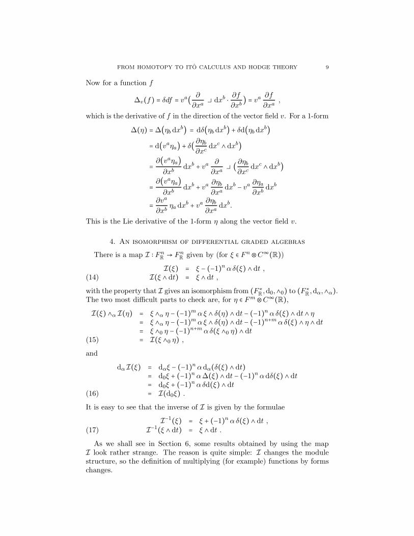
Now for a function f
∆v(f) = δdf = va( ∂
∂xa dxb ⋅ ∂f
∂xb) = va ∂f
∂xa,
which is the derivative of f in the direction of the vector field v. For a 1-form
As we shall see in Section 6, some results obtained by using the mapI look rather strange. The reason is quite simple: I changes the modulestructure, so the definition of multiplying (for example) functions by formschanges.
10 G. ALHAMZI, E.J. BEGGS & A.D. NEATE
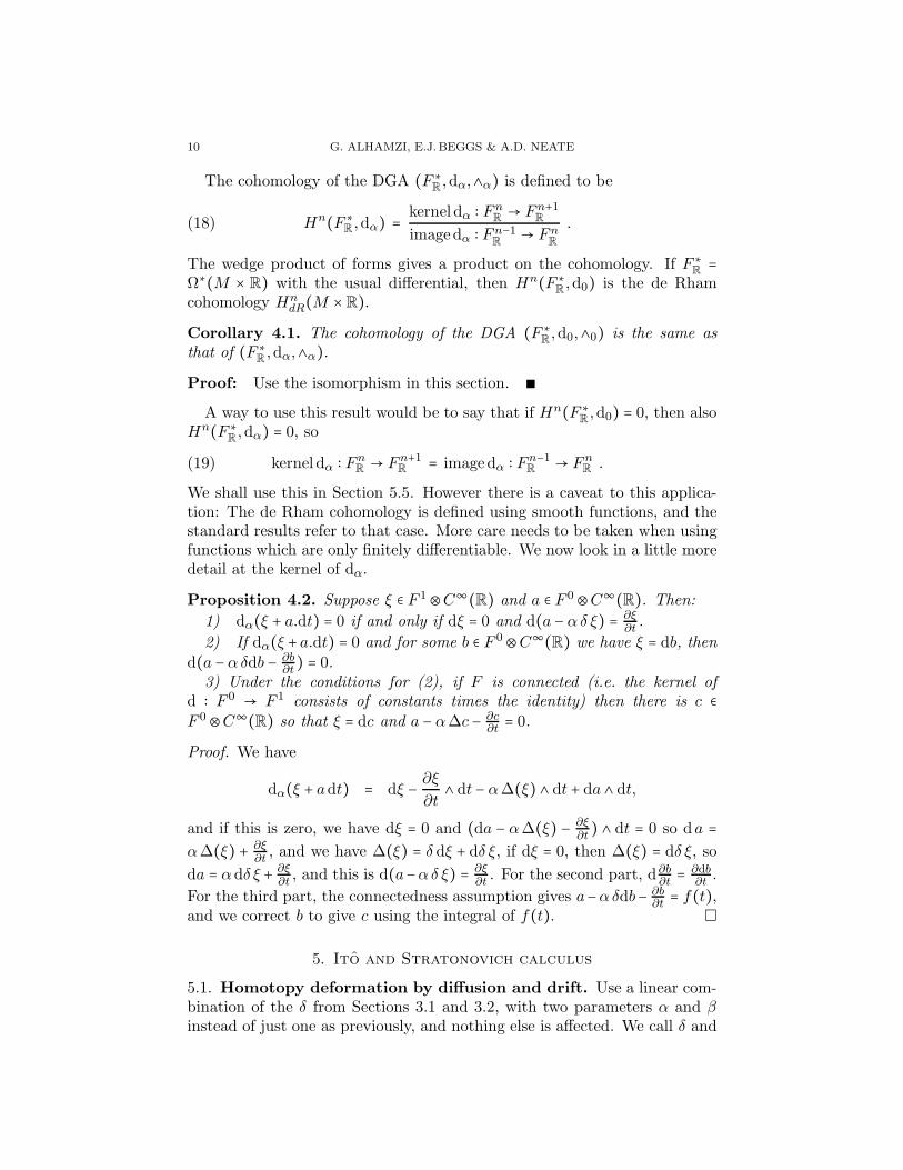
The cohomology of the DGA (F ∗R,dα,∧α) is defined to be
Hn(F ∗R ,dα) = kernel dα ∶ FnR→ Fn+1
R
imagedα ∶ Fn−1R→ Fn
R
.(18)
The wedge product of forms gives a product on the cohomology. If F ∗R=
Ω∗(M × R) with the usual differential, then Hn(F ∗R,d0) is the de Rham
cohomology HndR(M ×R).
Corollary 4.1. The cohomology of the DGA (F ∗R,d0,∧0) is the same as
that of (F ∗R,dα,∧α).
Proof: Use the isomorphism in this section. ∎A way to use this result would be to say that if Hn(F ∗
R,d0) = 0, then also
Hn(F ∗R,dα) = 0, so
kernel dα ∶ FnR → Fn+1
R = imagedα ∶ Fn−1R → Fn
R .(19)
We shall use this in Section 5.5. However there is a caveat to this applica-tion: The de Rham cohomology is defined using smooth functions, and thestandard results refer to that case. More care needs to be taken when usingfunctions which are only finitely differentiable. We now look in a little moredetail at the kernel of dα.
Proposition 4.2. Suppose ξ ∈ F 1⊗C∞(R) and a ∈ F 0⊗C∞(R). Then:
1) dα(ξ + a.dt) = 0 if and only if dξ = 0 and d(a − αδ ξ) = ∂ξ∂t.
2) If dα(ξ +a.dt) = 0 and for some b ∈ F 0⊗C∞(R) we have ξ = db, thend(a −αδdb − ∂b
∂t) = 0.
3) Under the conditions for (2), if F is connected (i.e. the kernel ofd ∶ F 0
→ F 1 consists of constants times the identity) then there is c ∈F 0⊗C∞(R) so that ξ = dc and a − α∆c − ∂c
∂t= 0.
Proof. We have
dα(ξ + adt) = dξ − ∂ξ
∂t∧ dt − α∆(ξ) ∧ dt + da ∧ dt,
and if this is zero, we have dξ = 0 and (da − α∆(ξ) − ∂ξ∂t) ∧ dt = 0 so da =
α∆(ξ) + ∂ξ∂t, and we have ∆(ξ) = δ dξ + dδ ξ, if dξ = 0, then ∆(ξ) = dδ ξ, so
da = αdδ ξ + ∂ξ∂t, and this is d(a−αδ ξ) = ∂ξ
∂t. For the second part, d∂b
∂t= ∂db
∂t.
For the third part, the connectedness assumption gives a−αδdb− ∂b∂t= f(t),
and we correct b to give c using the integral of f(t).
5. Ito and Stratonovich calculus
5.1. Homotopy deformation by diffusion and drift. Use a linear com-bination of the δ from Sections 3.1 and 3.2, with two parameters α and β
instead of just one as previously, and nothing else is affected. We call δ and
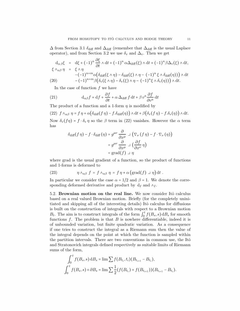
FROM HOMOTOPY TO ITO CALCULUS AND HODGE THEORY 11
∆ from Section 3.1 δdiff and ∆diff (remember that ∆diff is the usual Laplaceoperator), and from Section 3.2 we use δv and ∆v. Then we get
The product of a function and a 1-form η is modified by
(22) f ∧αβ η = f η +α(δdiff(f η)− f.δdiff(η)) ∧ dt+β(δv(f η)− f.δv(η))∧ dt.Now δv(fη) = f ⋅ δv η so the β term in (22) vanishes. However the α termhas
δdiff(f η) − f ⋅ δdiff (η) = gµν ∂
∂xµ (∇ν (f η) − f ⋅ ∇ν (η))
= gµν ∂
∂xµ ( ∂f
∂xνη)
= grad(f) η
where grad is the usual gradient of a function, so the product of functionsand 1-forms is deformed to
(23) η ∧αβ f = f ∧αβ η = f η + α (grad(f) η)dt .In particular we consider the case α = 1/2 and β = 1. We denote the corre-sponding deformed derivative and product by dI and ∧I .5.2. Brownian motion on the real line. We now consider Ito calculusbased on a real valued Brownian motion. Briefly (for the completely unini-tiated and skipping all of the interesting details) Ito calculus for diffusionsis built on the construction of integrals with respect to a Brownian motionBt. The aim is to construct integrals of the form ∫ t
0 f(Bs, s)dBs for smoothfunctions f . The problem is that B is nowhere differentiable, indeed it isof unbounded variation, but finite quadratic variation. As a consequenceif one tries to construct the integral as a Riemann sum then the value ofthe integral depends on the point at which the function is sampled withinthe partition intervals. There are two conventions in common use, the Itoand Stratonovich integrals defined respectively as suitable limits of Riemannsums of the form,
∫t
0f(Bs, s)dBs = lim∑f(Bti , ti)(Bti+1 −Bti),
∫t
0f(Bs, s) ∂Bs = lim∑ 1
2(f(Bti) + f(Bti+1))(Bti+1 −Bti).
12 G. ALHAMZI, E.J. BEGGS & A.D. NEATE
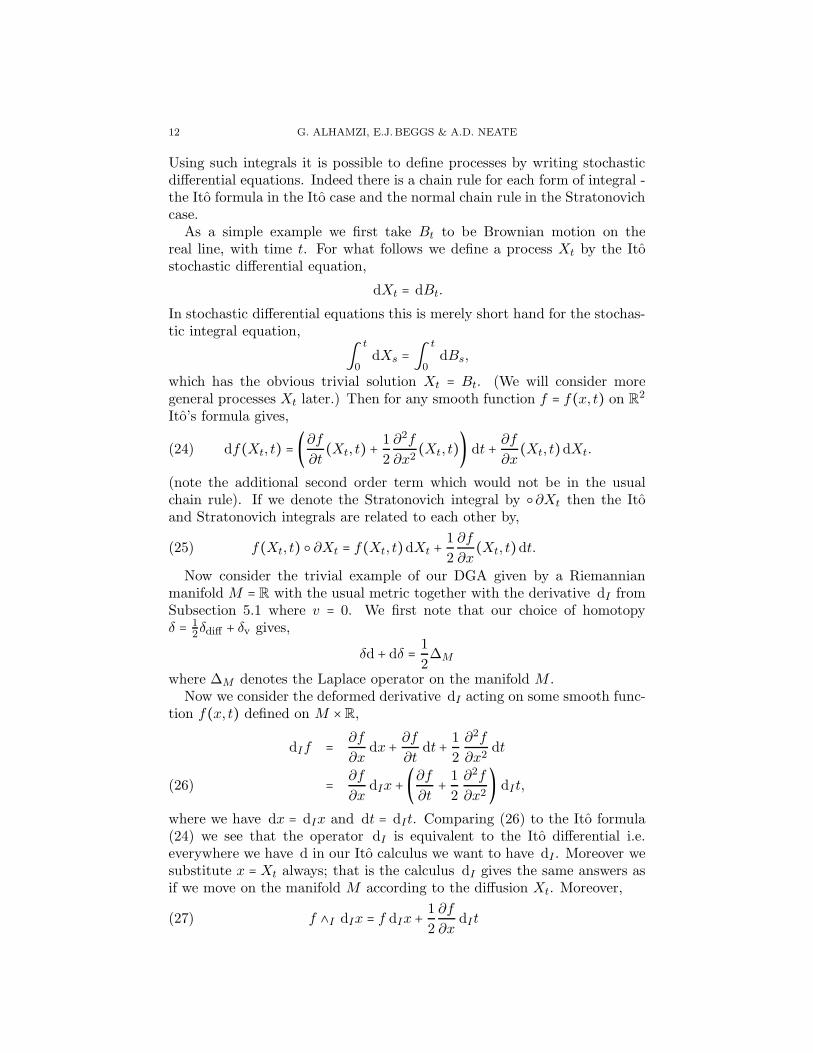
Using such integrals it is possible to define processes by writing stochasticdifferential equations. Indeed there is a chain rule for each form of integral -the Ito formula in the Ito case and the normal chain rule in the Stratonovichcase.
As a simple example we first take Bt to be Brownian motion on thereal line, with time t. For what follows we define a process Xt by the Itostochastic differential equation,
dXt = dBt.
In stochastic differential equations this is merely short hand for the stochas-tic integral equation,
∫t
0dXs = ∫ t
0dBs,
which has the obvious trivial solution Xt = Bt. (We will consider moregeneral processes Xt later.) Then for any smooth function f = f(x, t) on R
2
Ito’s formula gives,
(24) df(Xt, t) = (∂f∂t(Xt, t) + 1
2
∂2f
∂x2(Xt, t)) dt + ∂f
∂x(Xt, t)dXt.
(note the additional second order term which would not be in the usualchain rule). If we denote the Stratonovich integral by ∂Xt then the Itoand Stratonovich integrals are related to each other by,
f(Xt, t) ∂Xt = f(Xt, t)dXt + 1
2
∂f
∂x(Xt, t)dt.(25)
Now consider the trivial example of our DGA given by a Riemannianmanifold M = R with the usual metric together with the derivative dI fromSubsection 5.1 where v = 0. We first note that our choice of homotopyδ = 1
2δdiff + δv gives,
δd + dδ = 1
2∆M
where ∆M denotes the Laplace operator on the manifold M .Now we consider the deformed derivative dI acting on some smooth func-
tion f(x, t) defined on M ×R,dIf = ∂f
∂xdx + ∂f
∂tdt + 1
2
∂2f
∂x2dt
= ∂f
∂xdIx + (∂f
∂t+ 1
2
∂2f
∂x2) dIt,(26)
where we have dx = dIx and dt = dIt. Comparing (26) to the Ito formula(24) we see that the operator dI is equivalent to the Ito differential i.e.everywhere we have d in our Ito calculus we want to have dI . Moreover wesubstitute x = Xt always; that is the calculus dI gives the same answers asif we move on the manifold M according to the diffusion Xt. Moreover,
f ∧I dIx = f dIx + 1
2
∂f
∂xdIt(27)
FROM HOMOTOPY TO ITO CALCULUS AND HODGE THEORY 13
Thus we can see that the natural interpretation is for dI to be the Itodifferential whilst f ∧I dIx denotes the Stratonovich integral.
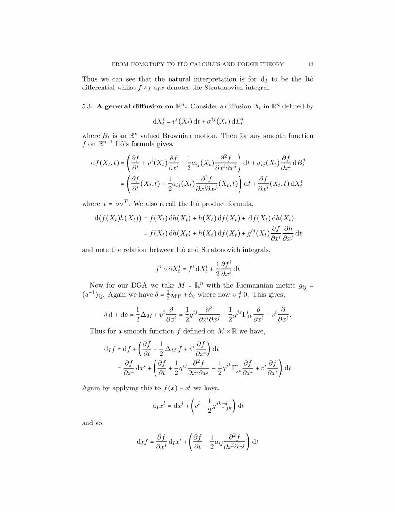
5.3. A general diffusion on Rn. Consider a diffusion Xt in R
n defined by
dXit = vi(Xt)dt + σij(Xt)dBj
t
where Bt is an Rn valued Brownian motion. Then for any smooth function
f on Rn+1 Ito’s formula gives,
df(Xt, t) = (∂f∂t+ vi(Xt) ∂f
∂xi+ 1
2aij(Xt) ∂2f
∂xi∂xj) dt + σij(Xt) ∂f
∂xidBj
t
= (∂f∂t(Xt, t) + 1
2aij(Xt) ∂2f
∂xi∂xj(Xt, t)) dt + ∂f
∂xi(Xt, t)dXi
t
where a = σσT . We also recall the Ito product formula,
and note the relation between Ito and Stratonovich integrals,
f i ∂Xit = f i dXi
t + 1
2
∂f i
∂xidt
Now for our DGA we take M = Rn with the Riemannian metric gij =(a−1)ij . Again we have δ = 1
2δdiff + δv where now v /≡ 0. This gives,
δ d + dδ = 1
2∆M + vi ∂
∂xi= 1
2gij
∂2
∂xi∂xj− 1
2gjkΓi
jk
∂
∂xi+ vi ∂
∂xi.
Thus for a smooth function f defined on M ×R we have,
dIf = df + (∂f∂t+ 1
2∆M f + vi ∂f
∂xi) dt
= ∂f
∂xidxi + (∂f
∂t+ 1
2gij
∂2f
∂xi∂xj− 1
2gjkΓi
jk
∂f
∂xi+ vi ∂f
∂xi) dt
Again by applying this to f(x) = xl we have,
dIxl = dxl + (vl − 1
2gjkΓl
jk) dtand so,
dIf = ∂f
∂xidIx
i + (∂f∂t+ 1
2aij
∂2f
∂xi∂xj) dt
14 G. ALHAMZI, E.J. BEGGS & A.D. NEATE
Also we note that,
f i ∧I dIxi = f i ∧I dxl + (f i ∧ (vl − 1
2gjkΓl
jk)) ∧ dt
= f i dxi + 1
2
∂f i
∂xidt + f i (vl − 1
2gjkΓl
jk) dt= f i dIx
i + 1
2
∂f i
∂xidt,
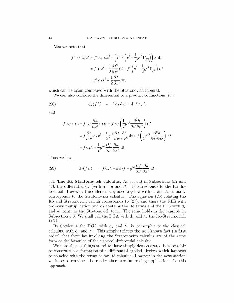
which can be again compared with the Stratonovich integral.We can also consider the differential of a product of functions f,h:
dI(f h) = f ∧I dIh + dIf ∧I h(28)
and
f ∧I dIh = f ∧I ∂h
∂xidIx
i + f ∧I (12gij
∂2h
∂xi∂xj) dt
= f ∂h
∂xidIx
i + 1
2gik
∂f
∂xi∂h
∂xkdt + f (1
2gij
∂2h
∂xi∂xj) dt
= f dIh + 1
2gik
∂f
∂xi∂h
∂xkdt.
Thus we have,
dI(f h) = f dIh + hdIf + gik ∂f
∂xi∂h
∂xkdt.(29)
5.4. The Ito-Stratonovich calculus. As set out in Subsections 5.2 and5.3, the differential dI (with α = 1
2and β = 1) corresponds to the Ito dif-
ferential. However, the differential graded algebra with dI and ∧I actuallycorresponds to the Stratonovich calculus. The equation (25) relating theIto and Stratonovich calculi corresponds to (27), and there the RHS withordinary multiplication and dI contains the Ito terms and the LHS with dIand ∧I contains the Stratonovich term. The same holds in the example inSubsection 5.3. We shall call the DGA with dI and ∧I the Ito-StratonovichDGA.
By Section 4 the DGA with dI and ∧I is isomorphic to the classicalcalculus, with d0 and ∧0. This simply reflects the well known fact (in firstorder) that formulae involving the Stratonovich calculus are of the sameform as the formulae of the classical differential calculus.
We note that as things stand we have simply demonstrated it is possibleto construct a deformation of a differential graded algebra which happensto coincide with the formulas for Ito calculus. However in the next sectionwe hope to convince the reader there are interesting applications for thisapproach.
FROM HOMOTOPY TO ITO CALCULUS AND HODGE THEORY 15
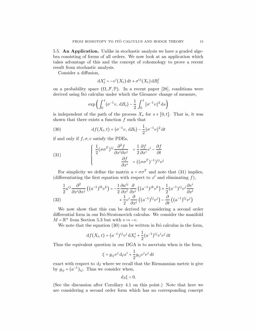
5.5. An Application. Unlike in stochastic analysis we have a graded alge-bra consisting of forms of all orders. We now look at an application whichtakes advantage of this and the concept of cohomology to prove a recentresult from stochastic analysis.
Consider a diffusion,
dXit = −vi(Xt)dt + σij(Xt)dBj
t
on a probability space (Ω,F ,P). In a recent paper [28], conditions werederived using Ito calculus under which the Girsanov change of measure,
exp(∫ t
0⟨σ−1v, dBs⟩ − 1
2 ∫t
0∥σ−1v∥2 ds)
is independent of the path of the process Xs for s ∈ [0, t]. That is, it wasshown that there exists a function f such that
(30) df(Xt, t) = ⟨σ−1v, dBt⟩ − 1
2∥σ−1v∥2 dt
if and only if f,σ, v satisfy the PDEs,
(31)
⎧⎪⎪⎪⎪⎪⎨⎪⎪⎪⎪⎪⎩
1
2(σσT )ij ∂2f
∂xi∂xj= 1
2
∂f
∂xivi − ∂f
∂t
∂f
∂xi= ((σσT )−1)ijvj
For simplicity we define the matrix a = σσT and note that (31) implies,(differentiating the first equation with respect to xl and eliminating f),
1
2aij
∂2
∂xi∂xj((a−1)lkvk) = −1
2
∂aij
∂xl∂
∂xi((a−1)jkvk) + 1
2(a−1)ijvj ∂vi
∂xl
+ 1
2vi
∂
∂xi((a−1)ljvj) − ∂
∂t((a−1)ljvj)(32)
We now show that this can be derived by considering a second orderdifferential form in our Ito-Stratonovich calculus. We consider the manifoldM = Rn from Section 5.3 but with v ↦ −v.
We note that the equation (30) can be written in Ito calculus in the form,
df(Xt, t) = (a−1)ijvj dXit + 1
2(a−1)ijvivj dt
Thus the equivalent question in our DGA is to ascertain when is the form,
ξ = gijvj dIxi + 1
2gijv
ivj dt
exact with respect to dI where we recall that the Riemannian metric is giveby gij = (a−1)ij . Thus we consider when,
dIξ = 0.(See the discussion after Corollary 4.1 on this point.) Note that here weare considering a second order form which has no corresponding concept
16 G. ALHAMZI, E.J. BEGGS & A.D. NEATE
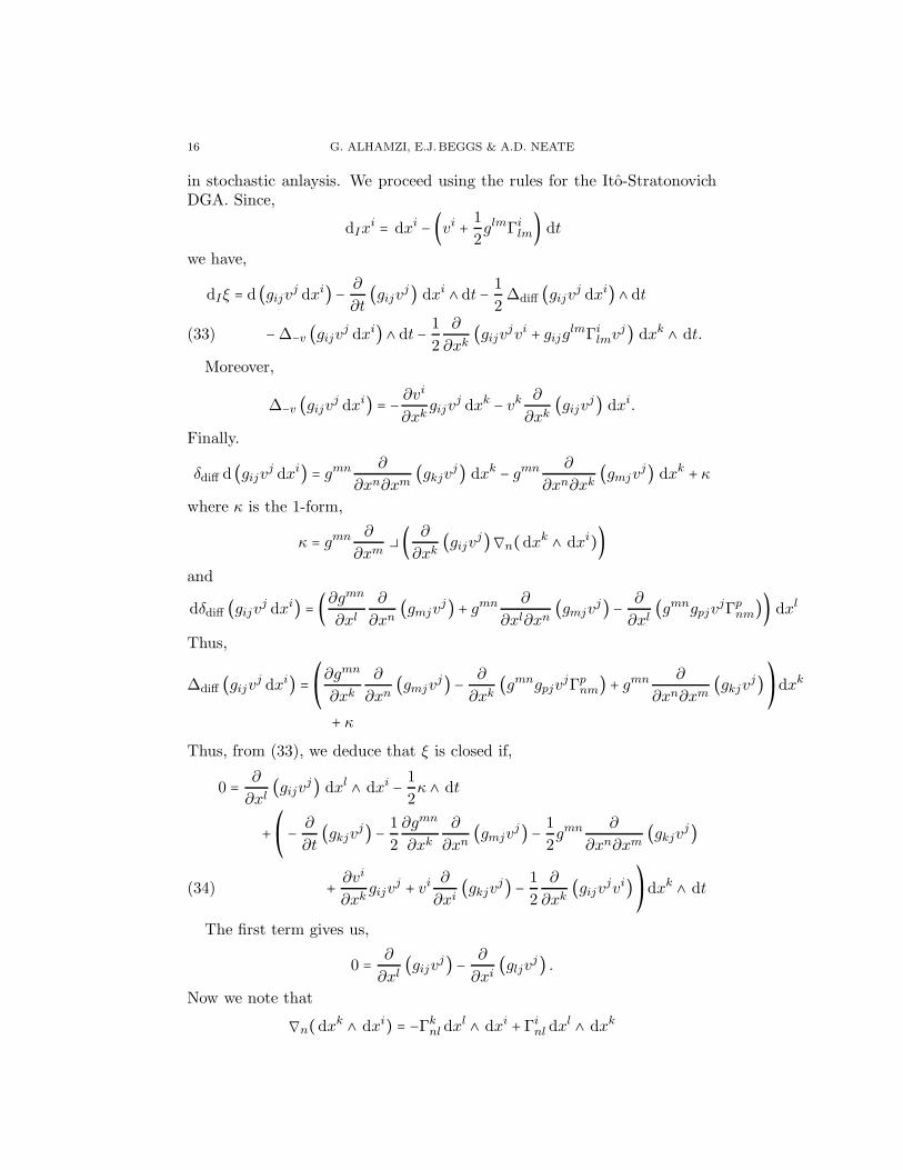
in stochastic anlaysis. We proceed using the rules for the Ito-StratonovichDGA. Since,
dIxi = dxi − (vi + 1
2glmΓi
lm) dtwe have,
dIξ = d (gijvj dxi) − ∂
∂t(gijvj) dxi ∧ dt − 1
2∆diff (gijvj dxi) ∧ dt
−∆−v (gijvj dxi) ∧ dt − 1
2
∂
∂xk(gijvjvi + gijglmΓi
lmvj) dxk ∧ dt.(33)
Moreover,
∆−v (gijvj dxi) = − ∂vi∂xk
gijvj dxk − vk ∂
∂xk(gijvj) dxi.
Finally.
δdiff d (gijvj dxi) = gmn ∂
∂xn∂xm(gkjvj) dxk − gmn ∂
∂xn∂xk(gmjv
j) dxk + κwhere κ is the 1-form,
κ = gmn ∂
∂xm ( ∂
∂xk(gijvj)∇n(dxk ∧ dxi))
and
dδdiff (gijvj dxi) = (∂gmn
∂xl∂
∂xn(gmjv
j) + gmn ∂
∂xl∂xn(gmjv
j) − ∂
∂xl(gmngpjv
jΓpnm)) dxl
Thus,
∆diff (gijvj dxi) = ⎛⎝∂gmn
∂xk∂
∂xn(gmjv
j) − ∂
∂xk(gmngpjv
jΓpnm) + gmn ∂
∂xn∂xm(gkjvj)⎞⎠dxk
+ κThus, from (33), we deduce that ξ is closed if,
0 = ∂
∂xl(gijvj) dxl ∧ dxi − 1
2κ ∧ dt
+ ⎛⎝ −∂
∂t(gkjvj) − 1
2
∂gmn
∂xk∂
∂xn(gmjv
j) − 1
2gmn ∂
∂xn∂xm(gkjvj)
+ ∂vi
∂xkgijv
j + vi ∂
∂xi(gkjvj) − 1
2
∂
∂xk(gijvjvi)⎞⎠dxk ∧ dt(34)
The first term gives us,
0 = ∂
∂xl(gijvj) − ∂
∂xi(gljvj) .
Now we note that
∇n(dxk ∧ dxi) = −Γknl dx
l ∧ dxi + Γinl dx
l ∧ dxk
FROM HOMOTOPY TO ITO CALCULUS AND HODGE THEORY 17
so that,
κ = gmn ∂
∂xm (− ∂
∂xk(gijvj)Γk
nl dxl ∧ dxi + ∂
∂xk(gijvj)Γi
nl dxl ∧ dxk)
= gmn (( ∂
∂xi(gkjvj) − ∂
∂xk(gijvj))Γk
nm + ( ∂
∂xk(gmjv
j) − ∂
∂xm(gkjvj))Γk
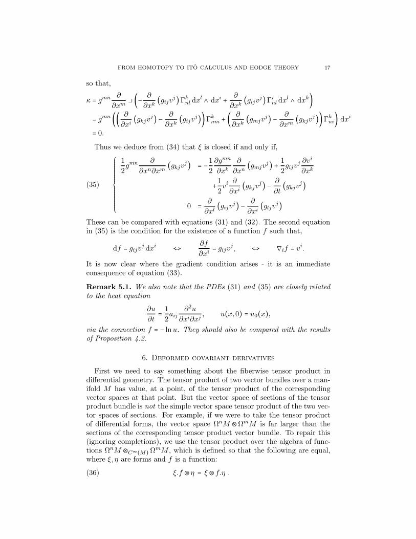
ni) dxi= 0.Thus we deduce from (34) that ξ is closed if and only if,
(35)
⎧⎪⎪⎪⎪⎪⎪⎪⎪⎪⎪⎪⎨⎪⎪⎪⎪⎪⎪⎪⎪⎪⎪⎪⎩
1
2gmn ∂
∂xn∂xm(gkjvj) = −1
2
∂gmn
∂xk∂
∂xn(gmjv
j) + 1
2gijv
j ∂vi
∂xk
+12vi
∂
∂xi(gkjvj) − ∂
∂t(gkjvj)
0 = ∂
∂xl(gijvj) − ∂
∂xi(gljvj)
These can be compared with equations (31) and (32). The second equationin (35) is the condition for the existence of a function f such that,
df = gijvj dxi ⇔
∂f
∂xi= gijvj , ⇔ ∇if = vi.
It is now clear where the gradient condition arises - it is an immediateconsequence of equation (33).
Remark 5.1. We also note that the PDEs (31) and (35) are closely relatedto the heat equation
∂u
∂t= 1
2aij
∂2u
∂xi∂xj, u(x,0) = u0(x),
via the connection f = − lnu. They should also be compared with the resultsof Proposition 4.2.
6. Deformed covariant derivatives
First we need to say something about the fiberwise tensor product indifferential geometry. The tensor product of two vector bundles over a man-ifold M has value, at a point, of the tensor product of the correspondingvector spaces at that point. But the vector space of sections of the tensorproduct bundle is not the simple vector space tensor product of the two vec-tor spaces of sections. For example, if we were to take the tensor productof differential forms, the vector space ΩnM ⊗ΩmM is far larger than thesections of the corresponding tensor product vector bundle. To repair this(ignoring completions), we use the tensor product over the algebra of func-tions ΩnM ⊗C∞(M)ΩmM , which is defined so that the following are equal,where ξ, η are forms and f is a function:
ξ.f ⊗η = ξ⊗f.η .(36)
18 G. ALHAMZI, E.J. BEGGS & A.D. NEATE
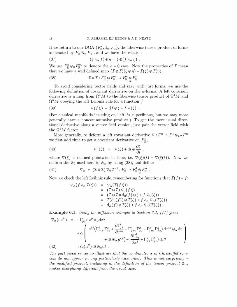
If we return to our DGA (F ∗R,dα,∧α), the fiberwise tensor product of forms
is denoted by FnR⊗α Fm
R, and we have the relation
(ξ ∧α f)⊗η = ξ⊗(f ∧α η) .(37)
We use FnR⊗0 Fm
Rto denote the α = 0 case. Now the properties of I mean
that we have a well defined map (I ⊗I)(ξ ⊗η) = I(ξ)⊗I(η),I ⊗I ∶ Fn
R ⊗0FmR → Fn
R ⊗αFmR .(38)
To avoid considering vector fields and stay with just forms, we use thefollowing definition of covariant derivative on the n-forms: A left covariantderivative is a map from ΩnM to the fiberwise tensor product of Ω1M andΩnM obeying the left Leibniz rule for a function f
∇(f.ξ) = df ⊗ ξ + f.∇(ξ) .(39)
(For classical manifolds insisting on ‘left’ is superfluous, but we may moregenerally have a noncommutative product.) To get the more usual direc-tional derivative along a vector field version, just pair the vector field withthe Ω1M factor.
More generally, to deform a left covariant derivative ∇ ∶ Fn→ F 1⊗F 0 Fn
we first add time to get a covariant derivative on FnR,
∇0(ξ) = ∇(ξ) + dt⊗ ∂ξ
∂t,(40)
where ∇(ξ) is defined pointwise in time, i.e. ∇(ξ)(t) = ∇(ξ(t)). Now wedeform the ⊗0 used here to ⊗α by using (38), and define
∇α = (I ⊗I)∇0 I−1 ∶ FnR → F 1
R⊗αFnR .(41)
Now we check the left Leibniz rule, remembering for functions that I(f) = f :∇α(f ∧α I(ξ)) = ∇α(I(f.ξ))= (I ⊗I)∇0(f.ξ)= (I ⊗I)(d0(f)⊗ ξ + f.∇0(ξ))= I(d0(f))⊗I(ξ) + f ∧α ∇α(I(ξ))= dα(f)⊗I(ξ) + f ∧α ∇α(I(ξ)) .
Example 6.1. Using the diffusion example in Section 3.1, (41) gives
∇α(dxk) = −Γkpq dx
p⊗αdxq
+α⎛⎜⎜⎜⎝
gi j(Γkms Γ
sj i +
∂Γkj i
∂xm− Γs
j m Γks i − Γs
im Γkj s)dxm⊗α dt
+dt⊗α gi j( − ∂Γki q
∂xj+ Γk
p q Γpj i)dxq
⎞⎟⎟⎟⎠+O(α2)dt⊗αdt .(42)
The part given serves to illustrate that the combinations of Christoffel sym-bols do not appear in any particularly nice order. This is not surprising –the modified product, including in the definition of the tensor product ⊗α,makes everything different from the usual case.
FROM HOMOTOPY TO ITO CALCULUS AND HODGE THEORY 19
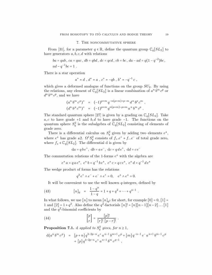
7. The noncommutative sphere
From [31], for a parameter q ∈ R, define the quantum group Cq[SL2] tohave generators a, b, c, d with relations
ba = qab , ca = qac , db = qbd , dc = qcd , cb = bc , da − ad = q(1 − q−2)bc ,ad − q−1bc = 1 .
There is a star operation
a∗ = d , d∗ = a , c∗ = −qb , b∗ = −q−1 c ,
which gives a deformed analogue of functions on the group SU2. By usingthe relations, any element of Cq[SL2] is a linear combination of an bm cp ordn bm cp, and we have
(an bm cp)∗ = (−1)p+m q−n(p+m)+p−m dn bp cm ,
(dn bp cm)∗ = (−1)p+m qn(p+m)−p+m an bm cp .
The standard quantum sphere [27] is given by a grading on Cq[SL2]. Takea, c to have grade +1 and b, d to have grade −1. The functions on thequantum sphere S2
q is the subalgebra of Cq[SL2] consisting of elements ofgrade zero.
There is a differential calculus on S2q given by adding two elements e±,
where e± has grade ±2. Ω1S2q consists of f+.e
+ + f−.e− of total grade zero,where f± ∈ Cq[SL2]. The differential d is given by
da = q b e+, db = ae−, dc = q de+, dd = c e−The commutation relations of the 1-forms e± with the algebra are
e± a = q a e±, e± b = q−1 b e±, e± c = q c e±, e± d = q−1 de±The wedge product of forms has the relations
q2 e+ ∧ e− + e− ∧ e+ = 0, e± ∧ e± = 0.It will be convenient to use the well known q-integers, defined by
In what follows, we use [n] to mean [n]q2 for short, for example [0] = 0, [1] =1 and [2] = 1+ q2. Also define the q2-factorials [n]! = [n][n− 1][n− 2] . . . [1]and the q2-binomial coefficients by
[pr] = [p]![r]! [p − r]! .(44)
Proposition 7.1. d applied to S2q gives, for n ≥ 1,
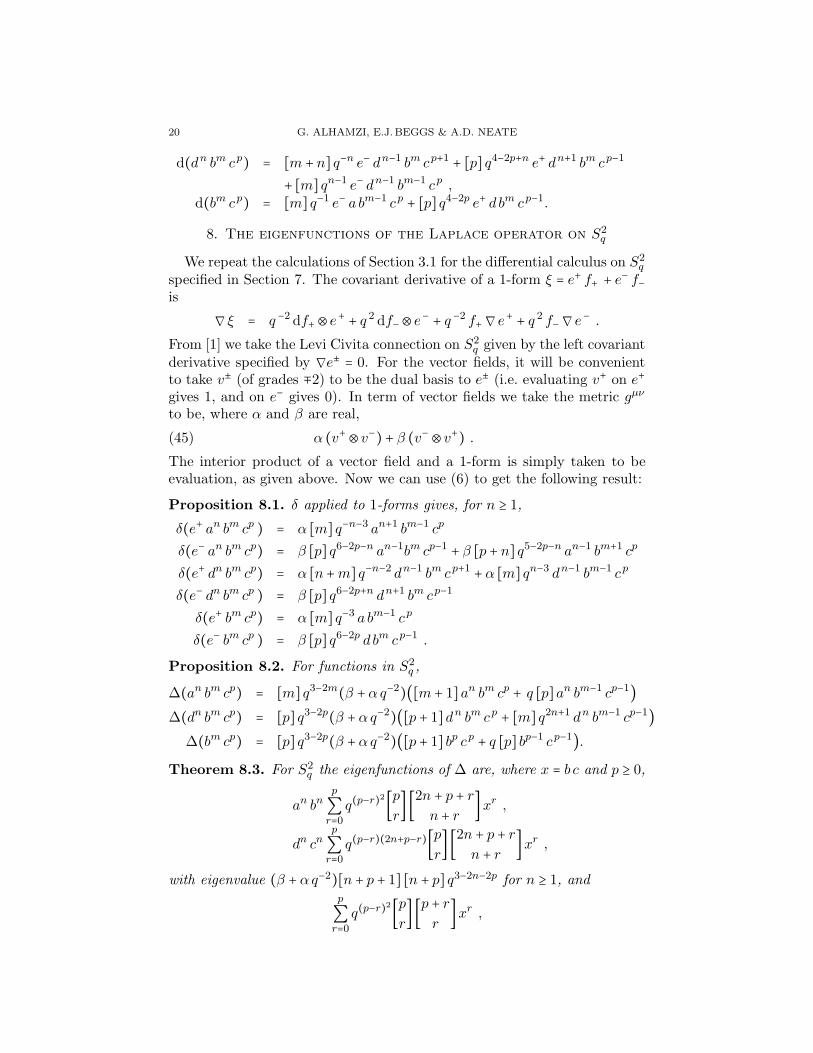
From [1] we take the Levi Civita connection on S2q given by the left covariant
derivative specified by ∇e± = 0. For the vector fields, it will be convenientto take v± (of grades ∓2) to be the dual basis to e± (i.e. evaluating v+ on e+
gives 1, and on e− gives 0). In term of vector fields we take the metric gµν
to be, where α and β are real,
α (v+⊗v−) + β (v−⊗v+) .(45)
The interior product of a vector field and a 1-form is simply taken to beevaluation, as given above. Now we can use (6) to get the following result:
∆(bm cp) = [p] q3−2p(β +αq−2)([p + 1] bp cp + q [p] bp−1 cp−1).Theorem 8.3. For S2
q the eigenfunctions of ∆ are, where x = b c and p ≥ 0,an bn
p
∑r=0
q(p−r)2[pr] [2n + p + r
n + r ]xr ,
dn cnp
∑r=0
q(p−r)(2n+p−r)[pr] [2n + p + r
n + r ]xr ,
with eigenvalue (β +αq−2)[n + p + 1] [n + p] q3−2n−2p for n ≥ 1, andp
∑r=0
q(p−r)2[pr] [p + r
r]xr ,
FROM HOMOTOPY TO ITO CALCULUS AND HODGE THEORY 21
with eigenvalue (β +αq−2)[p + 1] [p] q3−2p.
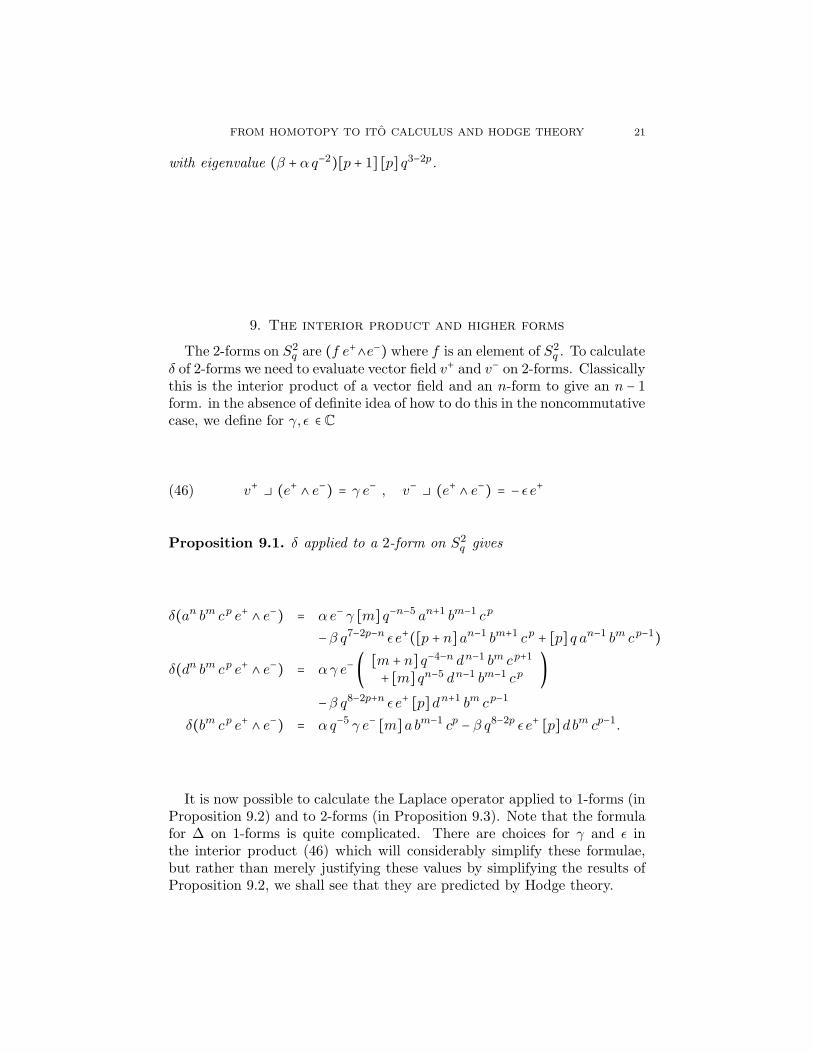
9. The interior product and higher forms
The 2-forms on S2q are (f e+∧e−) where f is an element of S2
q . To calculateδ of 2-forms we need to evaluate vector field v+ and v− on 2-forms. Classicallythis is the interior product of a vector field and an n-form to give an n − 1form. in the absence of definite idea of how to do this in the noncommutativecase, we define for γ, ǫ ∈ C
v+ (e+ ∧ e−) = γ e− , v− (e+ ∧ e−) = − ǫ e+(46)
Proposition 9.1. δ applied to a 2-form on S2q gives
It is now possible to calculate the Laplace operator applied to 1-forms (inProposition 9.2) and to 2-forms (in Proposition 9.3). Note that the formulafor ∆ on 1-forms is quite complicated. There are choices for γ and ǫ inthe interior product (46) which will considerably simplify these formulae,but rather than merely justifying these values by simplifying the results ofProposition 9.2, we shall see that they are predicted by Hodge theory.
Classically, the Hodge operator is a map ∶ ΩnM → Ωtop−nM , where topis the dimension of the manifold M . As we already have a star operation onthe algebra, it would be confusing to use star for the Hodge operation, asthey can both be applied to the same objects. On the manifold M we havean inner product for ΩnM given for η, ξ ∈ ΩnM
(47) ⟨η, ξ⟩ = ∫M(η ∧ ξ) .
FROM HOMOTOPY TO ITO CALCULUS AND HODGE THEORY 23
Here η ∧ ξ is a n+ (top −n) = top form. By Stokes’ theorem for orientatedM , for ξ ∈ ΩrM and η ∈ Ωr−1M ,
0 = ∫M
d(η ∧ ξ) = ∫M(dη) ∧ ξ − (−1)r ∫
Mη ∧ d( ξ) ,(48)
and this can be rewritten (assuming the invertibility of ) as⟨dη, ξ⟩ = (−1)r ⟨η,−1d ξ⟩ .(49)
A method for ensuring that the Laplacian is positive, which is taken classi-cally, is to take δ to the be the operator adjoint of d, i.e. for ξ ∈ ΩrM
δ(ξ) = (−1)r −1d ξ .(50)
We wish to use the Hodge operator on the noncommutative sphere. A read-ing of [21] will show that this operation has already been defined, but withdifferent formulae to the ones we will use. Our purposes differ from those of[21], where the Hodge operation was a module map. As we are interested infunctional analysis and positivity, our Hodge operation is conjugate linearto make (47) into a Hermitian inner product, in fact it is a module mapfrom ΩnS2
q to the conjugate module of Ωtop−nS2q .
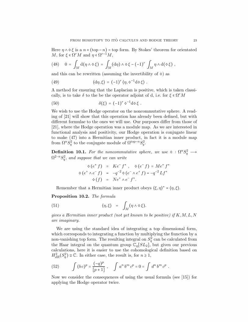
Definition 10.1. For the noncommutative sphere, we use ∶ ΩnS2q Ð→
Remember that a Hermitian inner product obeys ⟨ξ, η⟩∗ = ⟨η, ξ⟩.Proposition 10.2. The formula
⟨η, ξ⟩ = ∫M(η ∧ ξ).(51)
gives a Hermitian inner product (not yet known to be positive) if K,M,L,N
are imaginary.
We are using the standard idea of integrating a top dimensional form,which corresponds to integrating a function by multiplying the fiunction by anon-vanishing top form. The resulting integral on S2
q can be calculated fromthe Haar integral on the quantum group Cq[SL2], but given our previouscalculations, here it is easier to use the cohomological definition based onH2
dR(S2q ) ≅ C. In either case, the result is, for n ≥ 1,∫ (b c)p = (−q)p[p + 1] , ∫ an bm cp = 0 = ∫ dn bm cp .(52)
Now we consider the consequences of using the usual formula (see [15]) forapplying the Hodge operator twice.
24 G. ALHAMZI, E.J. BEGGS & A.D. NEATE
Proposition 10.3. The Hodge dual obeys
η = (−1)k(2−k) η.(53)
for all η ∈ ΩkS2q if and only if KM = 1 and LN = q2 in the Definition (10.1).
Now we compare the formula (50) for δ in terms of the Hodge operationwith the formulae in Proposition 9.1, which refer to the interior product in(46).
Proposition 10.4. For ξ ∈ ΩnS2q , the equation (−1)n δ ξ = d ξ is satisfied,
as long as the constants in (10.1) obey
α = K
Nq5 = L
γMq5 , β = −M
Nq−3 = − L
ǫKq−9 .
Corollary 10.5. To have (−1)n δ ξ = d ξ and ξ = (−1)n(2−n) ξ , forξ ∈ ΩnA for all n, we need for K,L imaginary,
α =KLq3, β = − L
Kq−5, γ = q2, ǫ = q−4,
Remark 10.6. The values of the constants derived from Hodge theory givea considerable simplification in the formulae for ∆, as noted in Section 11.While part of the reason may be that ∆ is self adjoint, there may also beanother reason, which might have a bearing on any probabilistic interpreta-tion. To use the heat equation in Brownian motion, there is one basic fact –the integral of a function is constant under the time evolution, correspond-ing to interpretation that no particle paths are lost or gained. In the innerproduct notation, the integral of a function f is ⟨f,1⟩, and saying that thisis conserved under the heat equation evolution corresponds to showing that⟨δdf,1⟩ = 0. If we use the fact that δ is the adjoint of d, this is ⟨df,d(1)⟩ = 0.
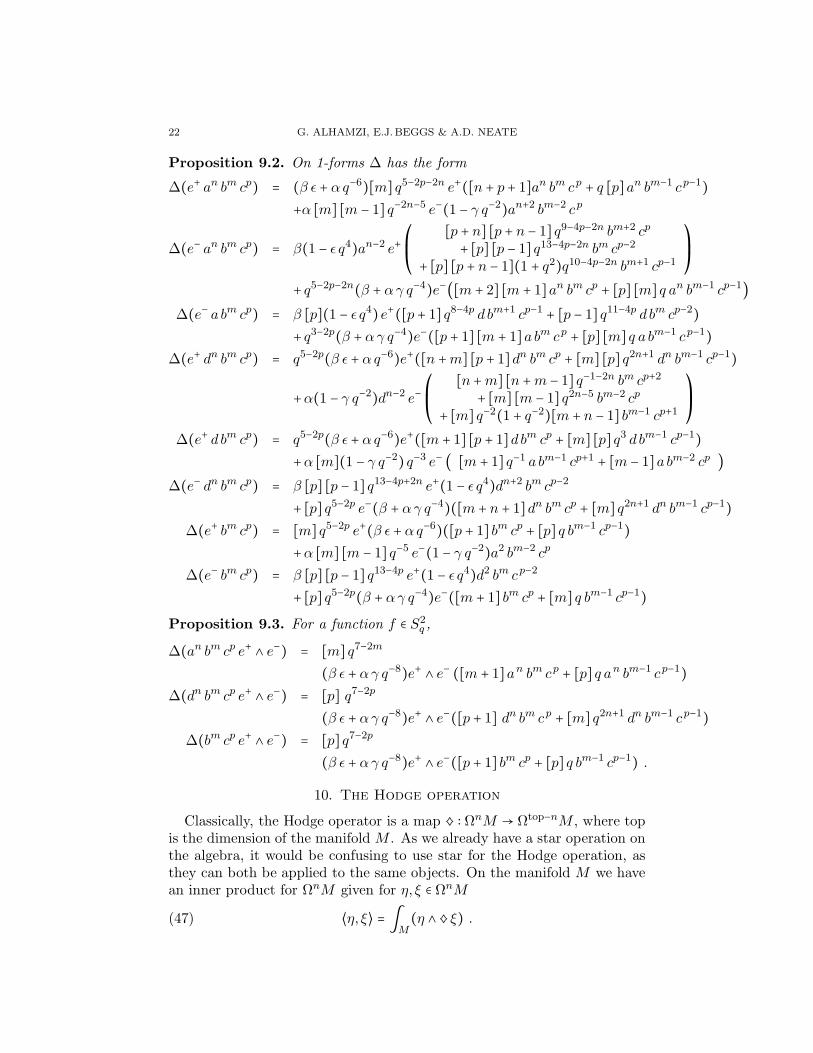
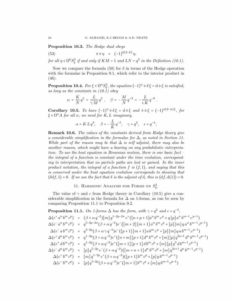
11. Harmonic Analysis for Forms on S2q .
The value of γ and ǫ from Hodge theory in Corollary (10.5) give a con-siderable simplification in the formula for ∆ on 1-forms, as can be seen bycomparing Proposition 11.1 to Proposition 9.2.
Proposition 11.1. On 1-forms ∆ has the form, with γ = q2 and ǫ = q−4,∆(e+ an bm cp) = (β +αq−2)[m] q1−2p−2n e+([n + p + 1]an bm cp + q [p]an bm−1 cp−1)∆(e− an bm cp) = q5−2p−2n(β + αq−2)e−([m + 2] [m + 1]an bm cp + [p] [m] q an bm−1 cp−1)∆(e− abm cp) = q3−2p(β + αγ q−4)e−([p + 1] [m + 1]abm cp + [p] [m] q a bm−1 cp−1)
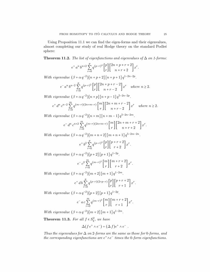
Using Proposition 11.1 we can find the eigen-forms and their eigenvalues,almost completing our study of real Hodge theory on the standard Podlessphere:
Theorem 11.2. The list of eigenfunctions and eigenvalues of ∆ on 1-forms:
e+ an bn+2p
∑r=0
q(p−r)2 [p
r] [2n + p + r + 2
n + r + 2 ]xr.With eigenvalue (β + αq−2)[n + p + 2] [n + p + 1] q1−2n−2p.
e− an bn−2p
∑r=0
q(p−r)2 [p
r] [2n + p + r − 2
n + r − 2 ]xr where n ≥ 2.With eigenvalue (β + αq−2)[n + p] [n + p − 1] q5−2n−2p.
e+ dn cn−2m
∑r=0
q(m−r)(2n+m−r) [mr] [2n +m + r − 2
n + r − 2 ]xr where n ≥ 2.With eigenvalue (β + αq−2)[n +m] [n +m − 1] q5−2n−2m.
e− dn cn+2m
∑r=0
q(m−r)(2n+m−r) [mr] [2n +m + r + 2
n + r + 2 ]xr.With eigenvalue (β + αq−2)[m + n + 2] [m + n + 1] q5−2m−2n.
Thus the eigenvalues for ∆ on 2-forms are the same as those for 0-forms, andthe corresponding eigenfunctions are e+∧e− times the 0-form eigenfunctions.
26 G. ALHAMZI, E.J. BEGGS & A.D. NEATE
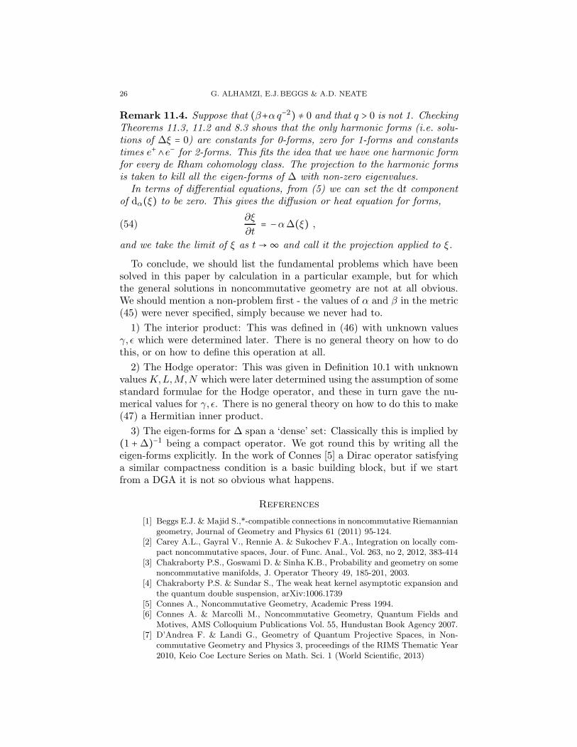
Remark 11.4. Suppose that (β+αq−2) ≠ 0 and that q > 0 is not 1. CheckingTheorems 11.3, 11.2 and 8.3 shows that the only harmonic forms (i.e. solu-tions of ∆ξ = 0) are constants for 0-forms, zero for 1-forms and constantstimes e+∧e− for 2-forms. This fits the idea that we have one harmonic formfor every de Rham cohomology class. The projection to the harmonic formsis taken to kill all the eigen-forms of ∆ with non-zero eigenvalues.
In terms of differential equations, from (5) we can set the dt componentof dα(ξ) to be zero. This gives the diffusion or heat equation for forms,
∂ξ
∂t= −α∆(ξ) ,(54)
and we take the limit of ξ as t →∞ and call it the projection applied to ξ.
To conclude, we should list the fundamental problems which have beensolved in this paper by calculation in a particular example, but for whichthe general solutions in noncommutative geometry are not at all obvious.We should mention a non-problem first - the values of α and β in the metric(45) were never specified, simply because we never had to.
1) The interior product: This was defined in (46) with unknown valuesγ, ǫ which were determined later. There is no general theory on how to dothis, or on how to define this operation at all.
2) The Hodge operator: This was given in Definition 10.1 with unknownvaluesK,L,M,N which were later determined using the assumption of somestandard formulae for the Hodge operator, and these in turn gave the nu-merical values for γ, ǫ. There is no general theory on how to do this to make(47) a Hermitian inner product.
3) The eigen-forms for ∆ span a ‘dense’ set: Classically this is implied by(1 +∆)−1 being a compact operator. We got round this by writing all theeigen-forms explicitly. In the work of Connes [5] a Dirac operator satisfyinga similar compactness condition is a basic building block, but if we startfrom a DGA it is not so obvious what happens.
References
[1] Beggs E.J. & Majid S.,*-compatible connections in noncommutative Riemanniangeometry, Journal of Geometry and Physics 61 (2011) 95-124.
[2] Carey A.L., Gayral V., Rennie A. & Sukochev F.A., Integration on locally com-pact noncommutative spaces, Jour. of Func. Anal., Vol. 263, no 2, 2012, 383-414
[3] Chakraborty P.S., Goswami D. & Sinha K.B., Probability and geometry on somenoncommutative manifolds, J. Operator Theory 49, 185-201, 2003.
[8] Das B. & Goswami D., Quantum Brownian Motion on Non-Commutative Mani-folds: Construction, Deformation and Exit Times Commun. Math. Physics 309,Issue 1, 193-228, 2012
[9] Dimakis A. & Muller-Hoissen F., Stochastic differential calculus, the Moyal *-product, and noncommutative geometry, Lett. in Math. Phys., Vol. 28, Issue 2,pp 123-137, 1993
[10] Elworthy K.D., Le Jan Y. & Li, Xue-Mei, On the Geometry of Diffusion Oper-ators and Stochastic Flows, Lect. Notes in Math., Vol. 1720, Springer 1999
[11] Elworthy K.D., Geometric aspects of diffusions on manifolds, Ecole d’te de Prob-abilites de Saint-Flour XV-XVII, 1985-87 Lecture Notes in Mathematics Volume1362, 1988, pp 277-425
[12] Elworthy K.D., Stochastic Differential Equations on Manifolds, LMS Lecturenote series 70, CUP 1982.
[13] Fiore G., Quantum group covariant (anti)symmetrizers, ǫ-tensors, vielbein,Hodge map and Laplacian, J. Phys. A: Math. Gen. 37 9175, 2004
[14] Gordina M., Stochastic differential equations on noncommutative L2, Finite andinfinite dimensional analysis in honor of Leonard Gross, eds. H-H. Kuo & A.N.Sengupta, Contemp. Math., 317 (2003), AMS Providence, RI, pp.87-98.
[15] Griffiths P. & Harris J., Principles of Algebraic Geometry, John Wiley & Sons,1978.
[16] Hudson R.L., Sticky shuffle Hopf algebras and their stochastic representations,pp165-181. in New trends in stochastic analysis and related topics, A volume in
honour of K D Elworthy, Ed H Zhao and A Truman, World Scientific (2012)[17] Hudson R.L., Ito calculus and quantisation of Lie bialgebras, Annales de
l’Institue H Poicare-PR 41 (P-A Meyer memorial volume), 375-390 (2005).[18] Hudson R.L. & Parthasarathy K.R., Deformations of algebras constructed using
quantum stochastic calculus, Lett. Math. Phys., 50: 115-133, 1999.[19] Ikeda N. &, Shinzo Watanabe S., Stochastic differential equations and diffusion
processes, North-Holland, 1989[20] Katzarkov L., Kontsevich M. &, Pantev T., Hodge theoretic aspects of mirror
symmetry Proceedings of Symposia in Pure Mathematics, Vol. 78, (2008), pp.87-174
[21] Majid S., Noncommutative Riemannian and Spin Geometry of the Standardq-Sphere , Comm. Math. Phys., June 2005, Volume 256, Issue 2, pp 255-285
[23] Malliavin P., Stochastic Analysis, Springer-Verlag, Berlin, 1997.[24] McKean H.P., Stochastic Integrals, Academic Press, N.Y. 1969.[25] Meyer P.A., A differential geometric formalism for the Ito calculus, Stochastic
Integrals Lecture Notes in Mathematics Volume 851, 1981, pp 256-270[26] Parthasarathy K.H., An Introduction to Quantum Stochastic Calculus,
Birkhauser, 1992.[27] Podles P., Quantum spheres, Lett. Math. Phys. 14, 193-202 (1987).[28] Truman A., Wang F., Wu J. & Yang W., A link of stochastic differential
equations to nonlinear parabolic equations, Sci. China Math., 55(10),1971–1976(2012)