57
1 Introduction to Bioinformatics for Computer Scientists Lecture 13
| Date post: | 17-Jan-2023 |
| Category: |
Documents |
| Upload: | khangminh22 |
| View: | 0 times |
| Download: | 0 times |
1
Introduction to Bioinformatics for Computer Scientists
Lecture 13

2
Plan for next lectures
● Today: advanced MCMC
● Tonight: course beers :-)
● Introduction to population genetics
● Course review
3
Outline for today
● Hastings correction
● Metropolis-coupled MCMC-methods
● Some phylogenetic MCMC proposals
● Reversible jump MCMC
4
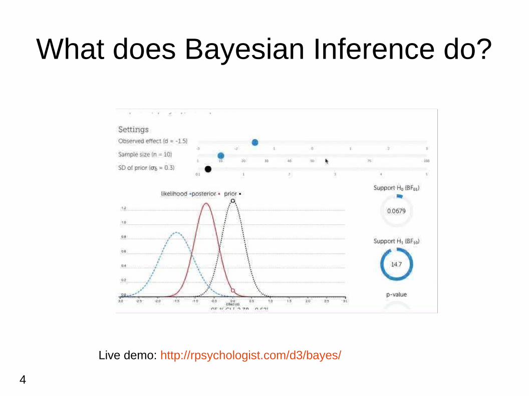
What does Bayesian Inference do?
Live demo: http://rpsychologist.com/d3/bayes/
5
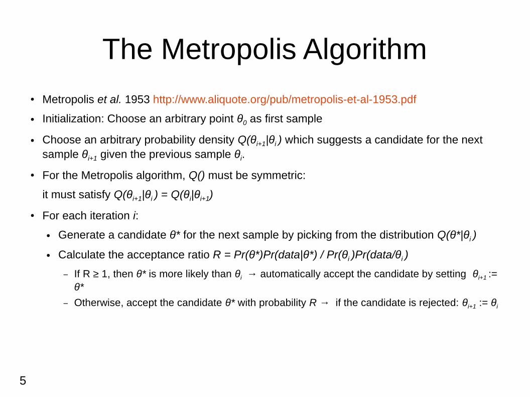
The Metropolis Algorithm
● Metropolis et al. 1953 http://www.aliquote.org/pub/metropolis-et-al-1953.pdf
● Initialization: Choose an arbitrary point θ0 as first sample
● Choose an arbitrary probability density Q(θi+1|θi ) which suggests a candidate for the next sample θi+1 given the previous sample θi.
● For the Metropolis algorithm, Q() must be symmetric:
it must satisfy Q(θi+1|θi ) = Q(θi|θi+1)
● For each iteration i:
● Generate a candidate θ* for the next sample by picking from the distribution Q(θ*|θi )
● Calculate the acceptance ratio R = Pr(θ*)Pr(data|θ*) / Pr(θi )Pr(data/θi )
– If R ≥ 1, then θ* is more likely than θi → automatically accept the candidate by setting θi+1 := θ*
– Otherwise, accept the candidate θ* with probability R → if the candidate is rejected: θi+1 := θi
6
The Metropolis Algorithm
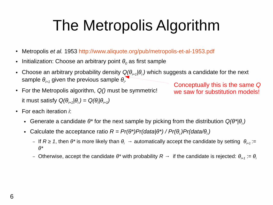
● Metropolis et al. 1953 http://www.aliquote.org/pub/metropolis-et-al-1953.pdf
● Initialization: Choose an arbitrary point θ0 as first sample
● Choose an arbitrary probability density Q(θi+1|θi ) which suggests a candidate for the next sample θi+1 given the previous sample θi.
● For the Metropolis algorithm, Q() must be symmetric!
it must satisfy Q(θi+1|θi ) = Q(θi|θi+1)
● For each iteration i:
● Generate a candidate θ* for the next sample by picking from the distribution Q(θ*|θi )
● Calculate the acceptance ratio R = Pr(θ*)Pr(data|θ*) / Pr(θi )Pr(data/θi )
– If R ≥ 1, then θ* is more likely than θi → automatically accept the candidate by setting θi+1 := θ*
– Otherwise, accept the candidate θ* with probability R → if the candidate is rejected: θi+1 := θi
Conceptually this is the same Qwe saw for substitution models!
7
The Metropolis Algorithm Phylogenetics
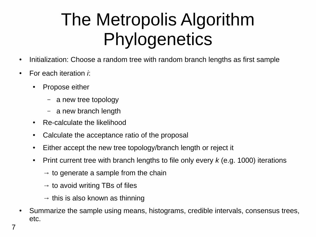
● Initialization: Choose a random tree with random branch lengths as first sample
● For each iteration i:
● Propose either
– a new tree topology
– a new branch length● Re-calculate the likelihood
● Calculate the acceptance ratio of the proposal
● Either accept the new tree topology/branch length or reject it
● Print current tree with branch lengths to file only every k (e.g. 1000) iterations
→ to generate a sample from the chain
→ to avoid writing TBs of files
→ this is also known as thinning
● Summarize the sample using means, histograms, credible intervals, consensus trees, etc.
8
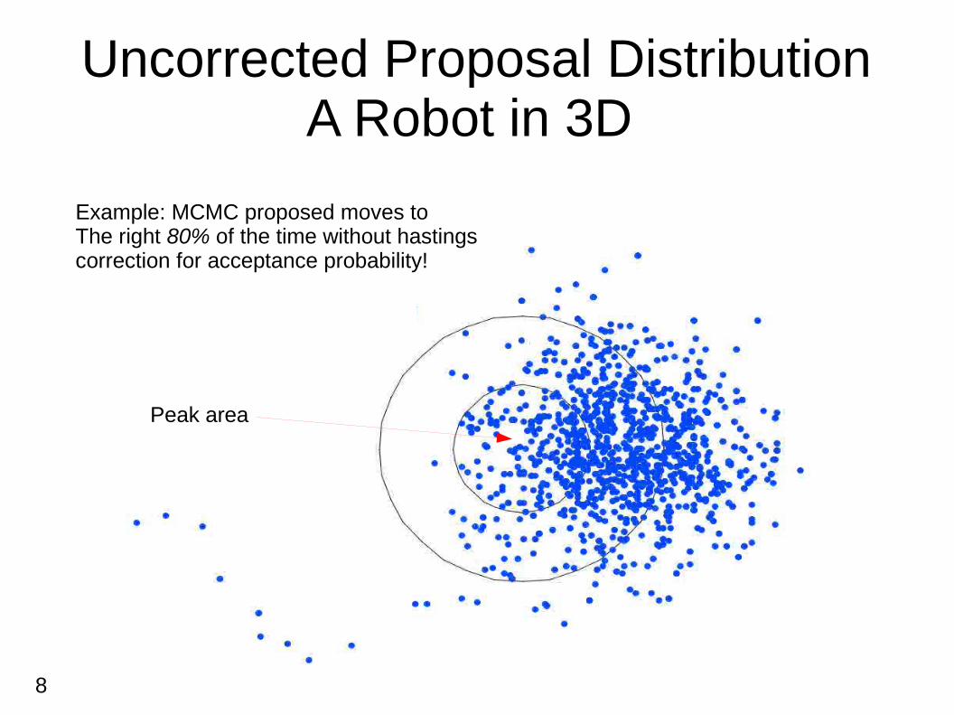
Uncorrected Proposal DistributionA Robot in 3D
Example: MCMC proposed moves toThe right 80% of the time without hastings correction for acceptance probability!
Peak area
9
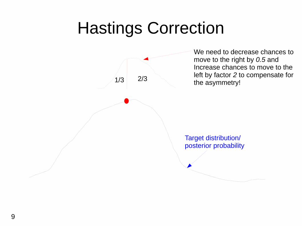
Hastings Correction
Target distribution/posterior probability
We need to decrease chances to move to the right by 0.5 and Increase chances to move to the left by factor 2 to compensate forthe asymmetry!1/3 2/3
10
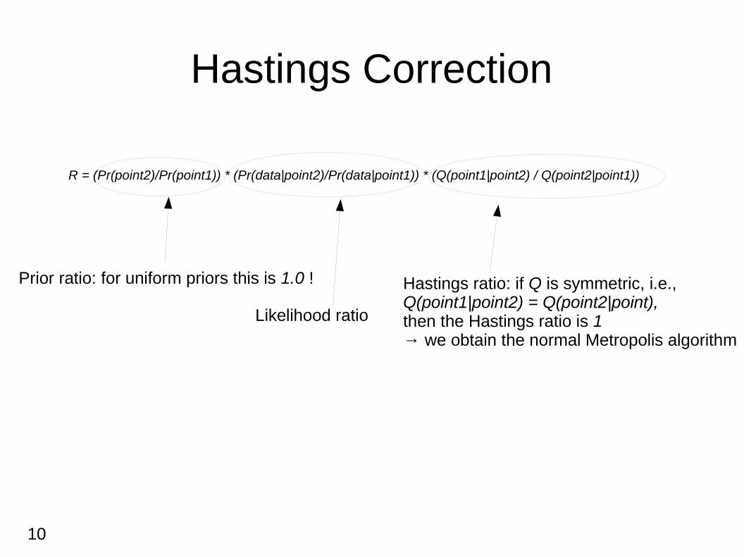
Hastings Correction
R = (Pr(point2)/Pr(point1)) * (Pr(data|point2)/Pr(data|point1)) * (Q(point1|point2) / Q(point2|point1))
Prior ratio: for uniform priors this is 1.0 !
Likelihood ratio
Hastings ratio: if Q is symmetric, i.e., Q(point1|point2) = Q(point2|point), then the Hastings ratio is 1 → we obtain the normal Metropolis algorithm
11
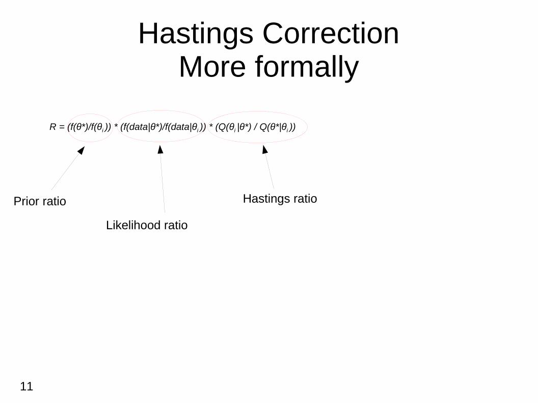
Hastings CorrectionMore formally
R = (f(θ*)/f(θi )) * (f(data|θ*)/f(data|θi )) * (Q(θi |θ*) / Q(θ*|θi ))
Prior ratio
Likelihood ratio
Hastings ratio
12
Hastings Correction is not trivial
● Problem with the equation for the hastings correction
● M. Holder, P. Lewis, D. Swofford, B. Larget. 2005. Hastings Ratio of the LOCAL Proposal Used in Bayesian Phylogenetics. Systematic Biology. 54:961-965. http://sysbio.oxfordjournals.org/content/54/6/961.full
“As part of another study, we estimated the marginal likelihoods of trees using different proposal algorithms and discovered repeatable discrepancies that implied that the published Hastings ratio for a proposal mechanism used in many Bayesian phylogenetic analyses is incorrect.”
● Incorrect Hastings ratio used from 1999-2005
13
Formal Method to derive the Hastings Ratio
● General method/algorithm for deriving the Hastings Ratio proposed by Peter Green
PJ Green. “Trans-dimensional markov chain monte carlo”. In: Oxford Statistical Science Series (2003), pp. 179–198.
● I will not go into the details
● Just remember that there exists such a method!
14
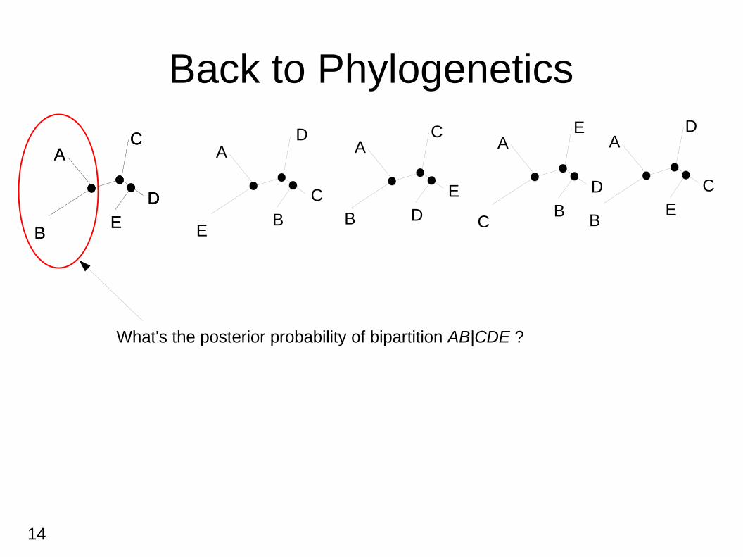
Back to Phylogenetics
A
B
C
D
E
A
B
C
D
E
AC
D
A
E
D
C
B
A
B
C
E
D
A
C
E
D
B
A
B
D
C
E
What's the posterior probability of bipartition AB|CDE ?
15
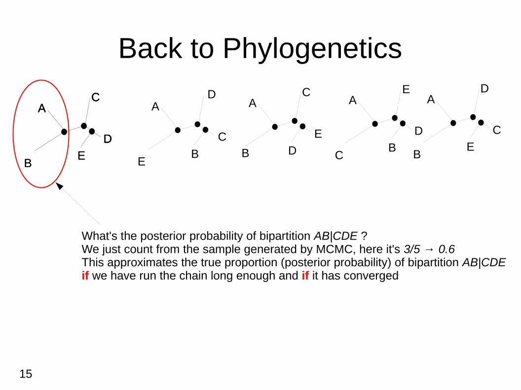
Back to Phylogenetics
A
B
C
D
E
A
B
C
D
E
AC
D
A
E
D
C
B
A
B
C
E
D
A
C
E
D
B
A
B
D
C
E
What's the posterior probability of bipartition AB|CDE ?We just count from the sample generated by MCMC, here it's 3/5 → 0.6This approximates the true proportion (posterior probability) of bipartition AB|CDE if we have run the chain long enough and if it has converged
16
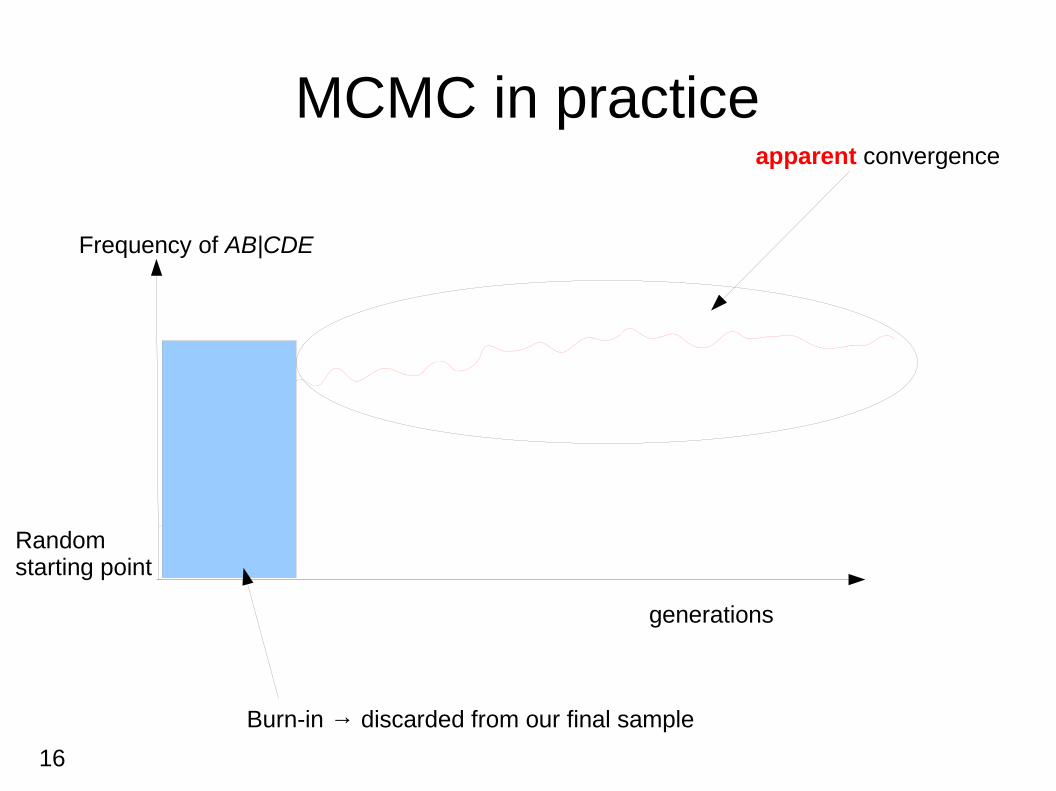
MCMC in practice
Frequency of AB|CDE
generations
apparent convergence
Burn-in → discarded from our final sample
Randomstarting point
17
Convergence
● How many samples do we need to draw to obtain an accurate approximation?
● When can we stop drawing samples?
● Methods for convergence diagnosis
→ we can never say that a MCMC-chain has converged
→ we can only diagnose that it has not converged
→ a plethora of tools for apparent convergence diagnostics for phylogenetic MCMC exist
18
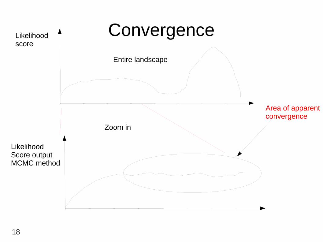
Convergence
Entire landscape
Likelihood score
Likelihood Score outputMCMC method
Area of apparentconvergence
Zoom in
19
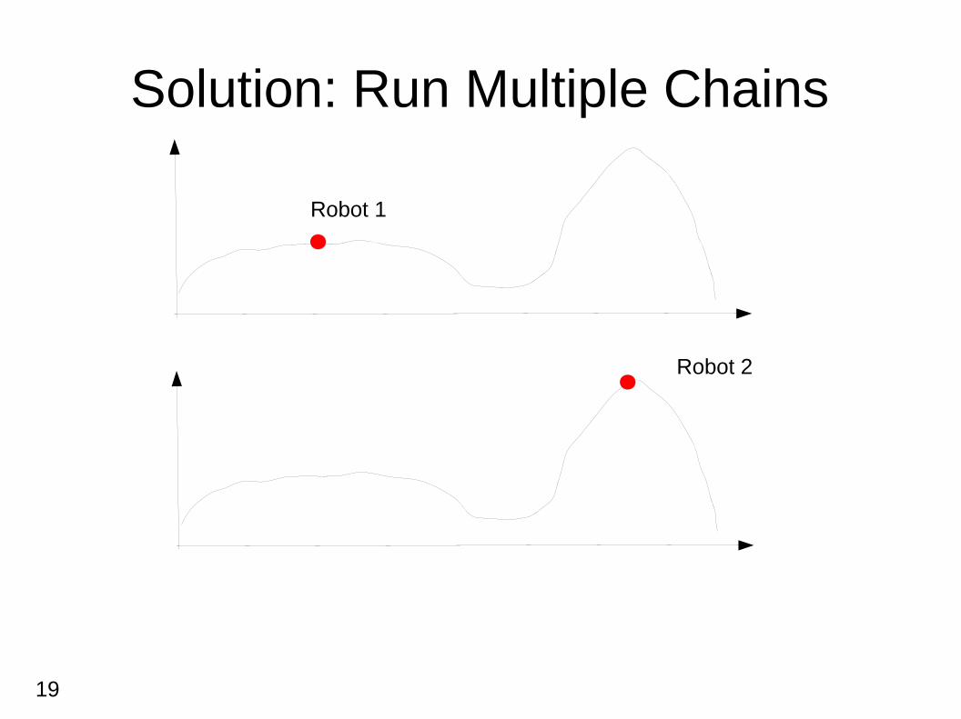
Solution: Run Multiple Chains
Robot 1
Robot 2
20
Outline for today
● Markov-Chain Monte-Carlo methods
● Metropolis-coupled MCMC-methods
● Some phylogenetic MCMC proposals
● Reversible jump MCMC
21
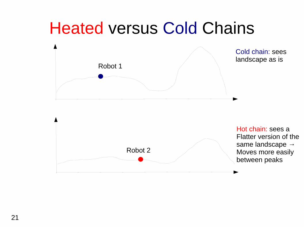
Heated versus Cold Chains
Robot 1
Robot 2
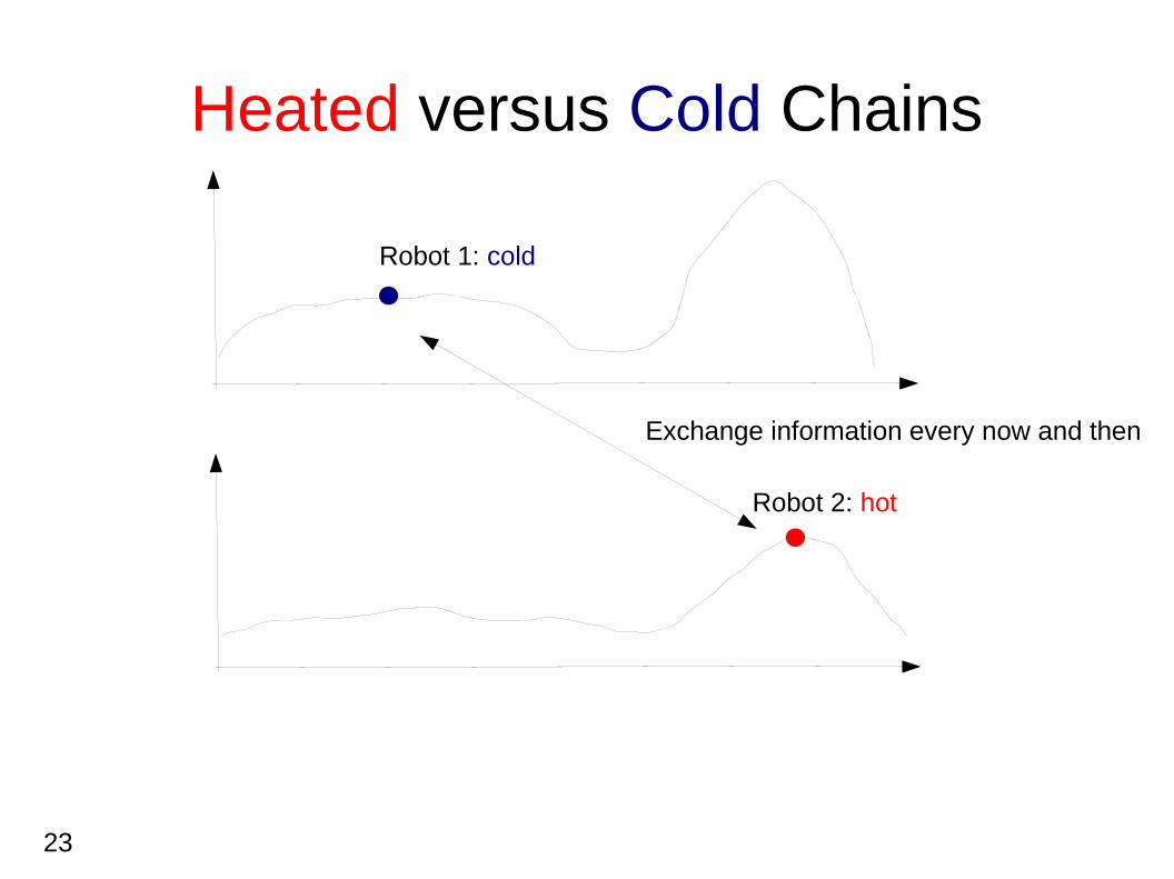
Cold chain: sees landscape as is
Hot chain: sees a Flatter version of the same landscape → Moves more easily between peaks
22
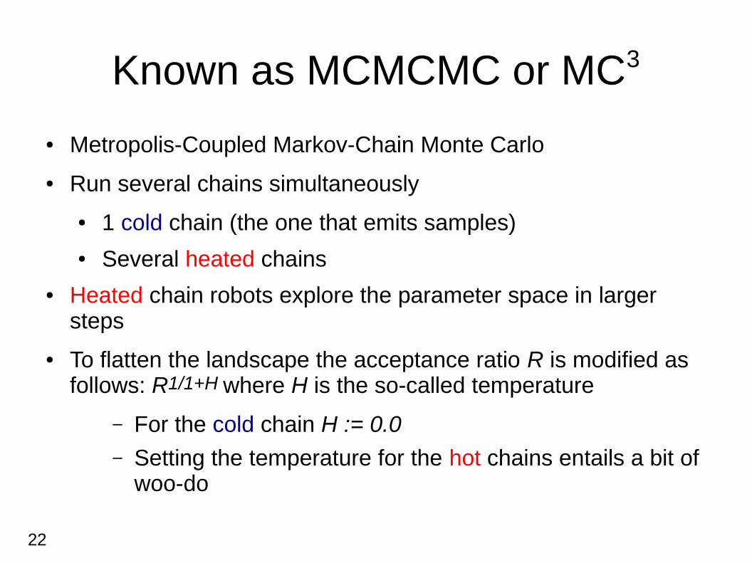
Known as MCMCMC or MC3
● Metropolis-Coupled Markov-Chain Monte Carlo
● Run several chains simultaneously
● 1 cold chain (the one that emits samples)● Several heated chains
● Heated chain robots explore the parameter space in larger steps
● To flatten the landscape the acceptance ratio R is modified as follows: R1/1+H where H is the so-called temperature
– For the cold chain H := 0.0– Setting the temperature for the hot chains entails a bit of
woo-do
23
Heated versus Cold Chains
Robot 1: cold
Robot 2: hot
Exchange information every now and then
24
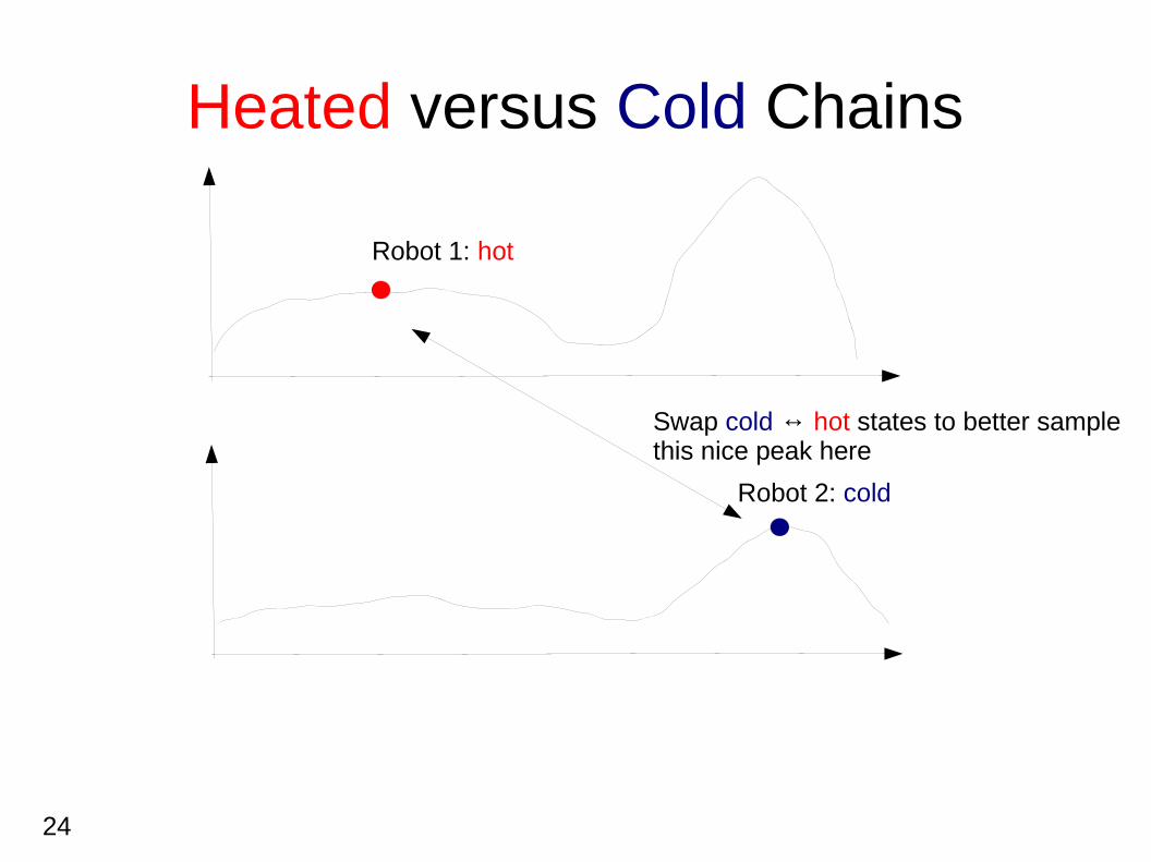
Heated versus Cold Chains
Robot 1: hot
Robot 2: cold
Swap cold ↔ hot states to better sample this nice peak here
25
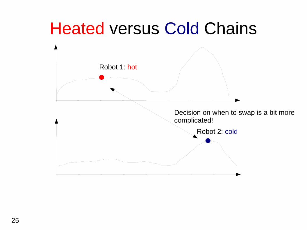
Heated versus Cold Chains
Robot 1: hot
Robot 2: cold
Decision on when to swap is a bit more complicated!
26
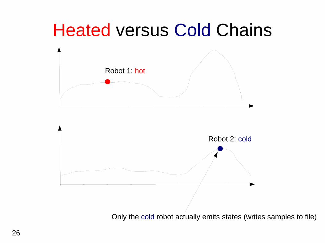
Heated versus Cold Chains
Robot 1: hot
Robot 2: cold
Only the cold robot actually emits states (writes samples to file)
27
A few words about priors
● Prior probabilities convey the scientist's beliefs, before having seen the data
● Using uninformative prior probability distributions (e.g., uniform priors, also called flat priors)
→ differences between prior and posterior distribution are attributable to likelihood differences only
● Priors can bias an analysis
● For instance, we could chose an arbitrary prior distribution for branch lengths in the range [1.0,20.0]
→ what happens if branch lengths are much shorter?
28
Outline for today
● Markov-Chain Monte-Carlo methods
● Metropolis-coupled MCMC-methods
● Some phylogenetic MCMC proposals
● Reversible jump MCMC

29
Some Phylogenetic Proposal Mechanisms
● Univariate parameters & branch lengths
● Sliding Window Proposal
● Branch lengths
● Node slider proposal
● Topologies
● Local Proposal (the one with the bug in the Hastings ratio!)
● Remember: We need to design proposals for which
● We either don't need to calculate the Hastings ratio
● Or for which we can calculate it
● That have an appropriate acceptance rate
→ all sorts of tricks being used, e.g., parsimony-biased topological proposals
→ acceptance rate should be around 25% (empirical observation)
→ for sampling from a multivariate normal distribution it has been shown that an acceptance rate of 23.4% is optimal
30
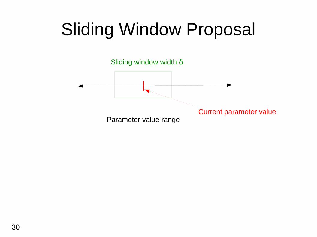
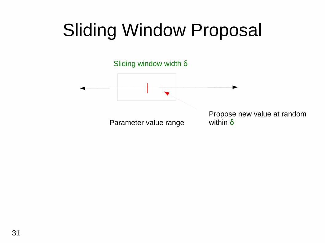
Sliding Window Proposal
Parameter value rangeCurrent parameter value
Sliding window width δ
31
Sliding Window Proposal
Parameter value range
Sliding window width δ
Propose new value at randomwithin δ
32
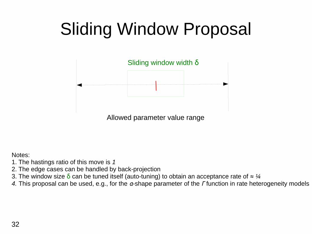
Sliding Window Proposal
Allowed parameter value range
Sliding window width δ
Notes: 1. The hastings ratio of this move is 12. The edge cases can be handled by back-projection3. The window size δ can be tuned itself (auto-tuning) to obtain an acceptance rate of ≈ ¼4. This proposal can be used, e.g., for the α-shape parameter of the Γ function in rate heterogeneity models
33
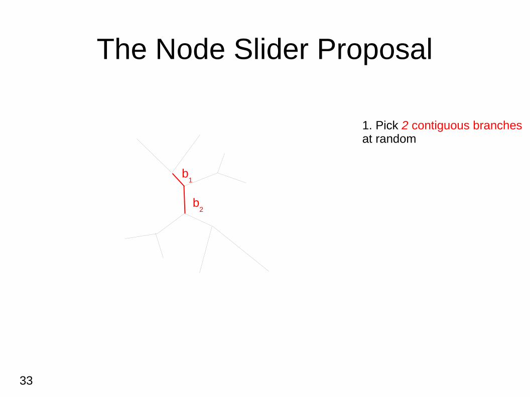
The Node Slider Proposal
1. Pick 2 contiguous branches at random
b1
b2
34
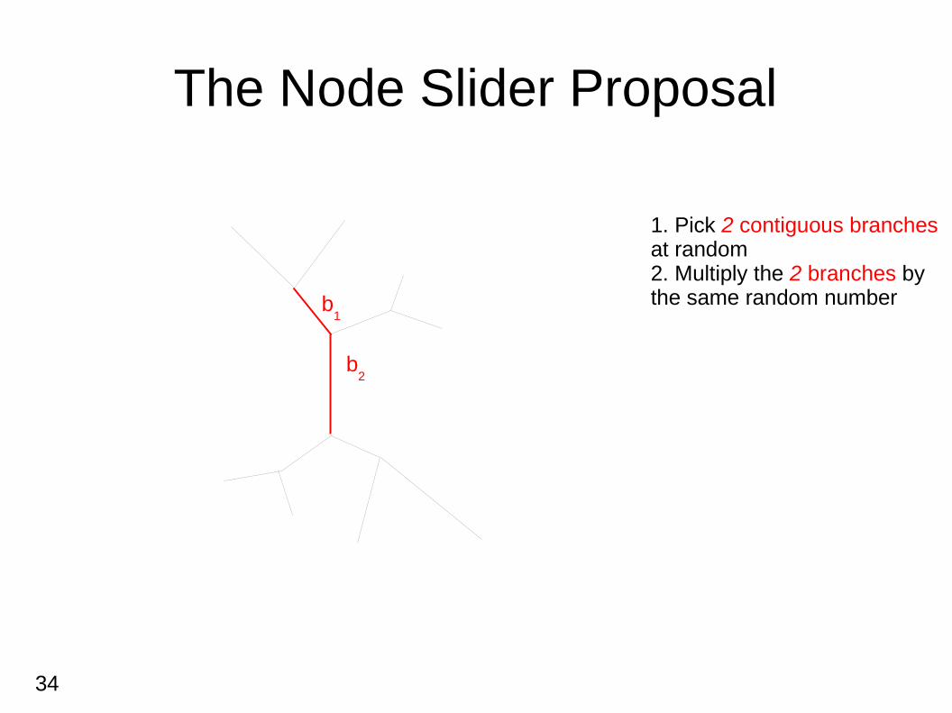
The Node Slider Proposal
1. Pick 2 contiguous branches at random2. Multiply the 2 branches by the same random number
b2
b1
35
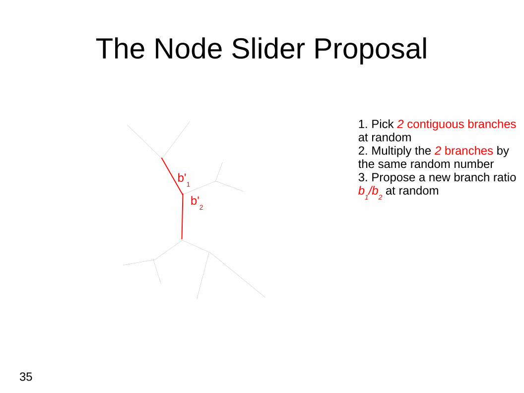
The Node Slider Proposal
1. Pick 2 contiguous branches at random2. Multiply the 2 branches by the same random number3. Propose a new branch ratio b
1/b
2 at random
b'1
b'2
36
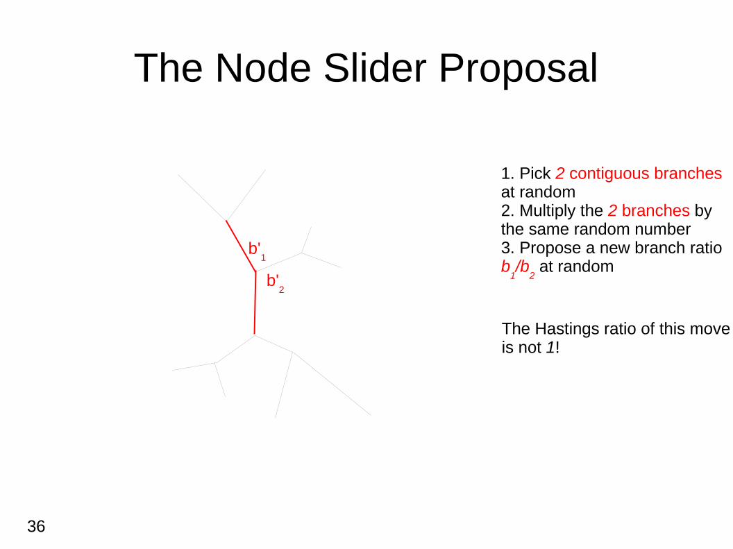
The Node Slider Proposal
1. Pick 2 contiguous branches at random2. Multiply the 2 branches by the same random number3. Propose a new branch ratio b
1/b
2 at random
b'1
b'2
The Hastings ratio of this moveis not 1!
37
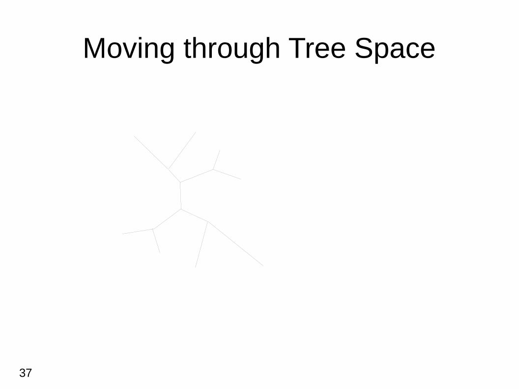
Moving through Tree Space
38
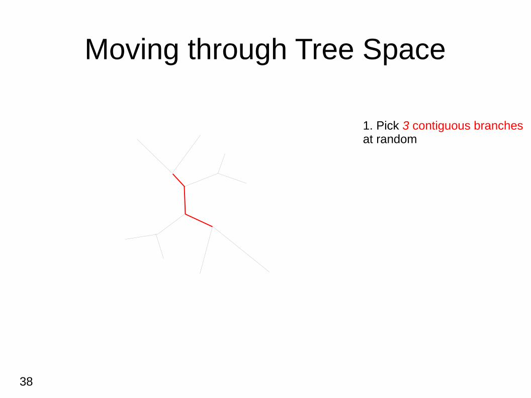
Moving through Tree Space
1. Pick 3 contiguous branches at random
39
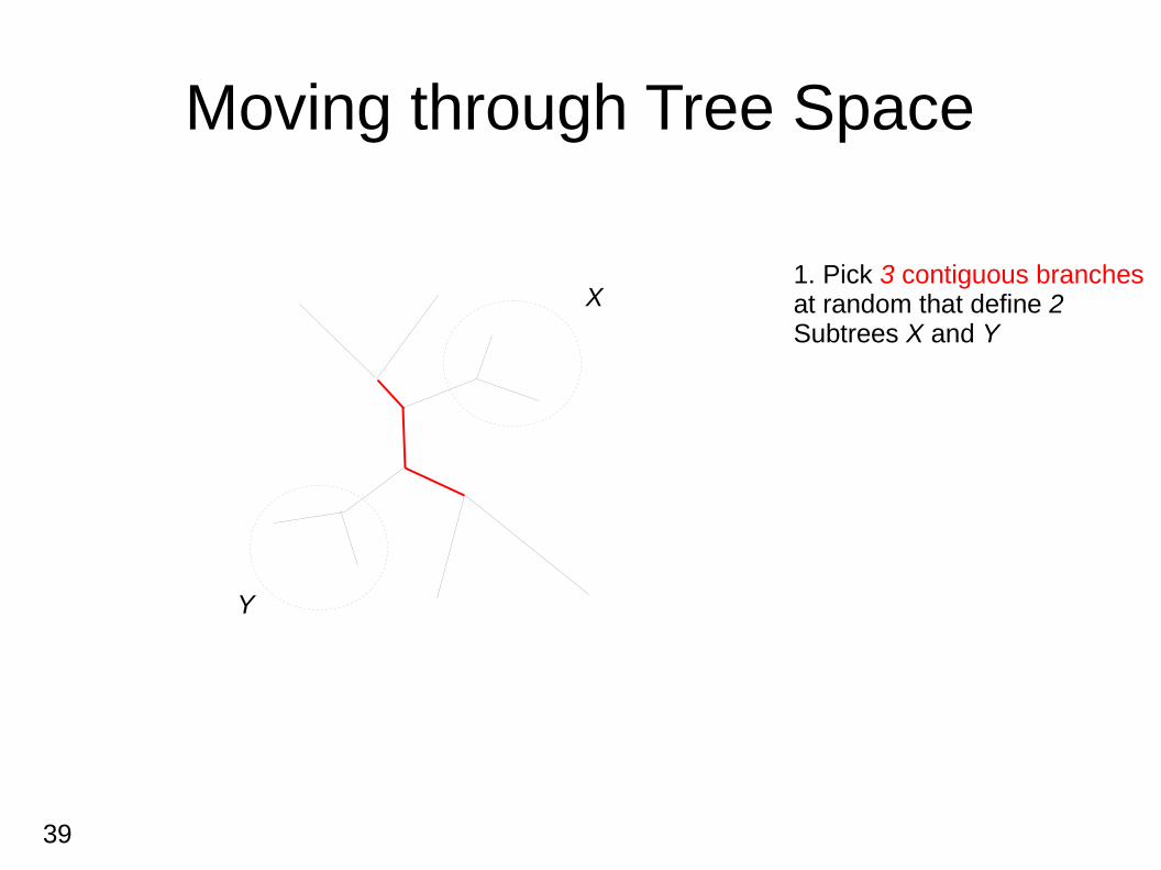
Moving through Tree Space
1. Pick 3 contiguous branches at random that define 2 Subtrees X and Y
X
Y

40
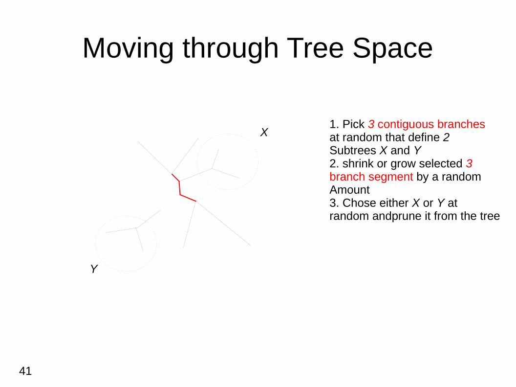
Moving through Tree Space
1. Pick 3 contiguous branches at random that define 2 Subtrees X and Y2. shrink or grow selected 3 branch segment by a random amount
X
Y
41
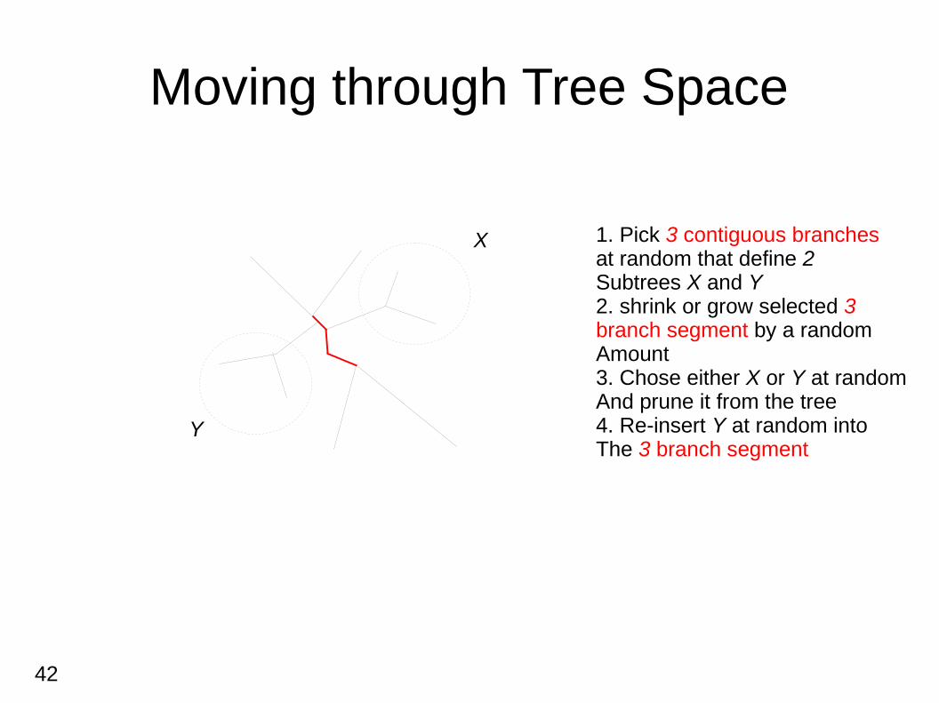
Moving through Tree Space
1. Pick 3 contiguous branches at random that define 2 Subtrees X and Y2. shrink or grow selected 3 branch segment by a random Amount3. Chose either X or Y at random andprune it from the tree
X
Y
42
Moving through Tree Space
1. Pick 3 contiguous branches at random that define 2 Subtrees X and Y2. shrink or grow selected 3 branch segment by a random Amount3. Chose either X or Y at random And prune it from the tree4. Re-insert Y at random intoThe 3 branch segment
X
Y
43
Moving through Tree Space
X
Y
X
Y
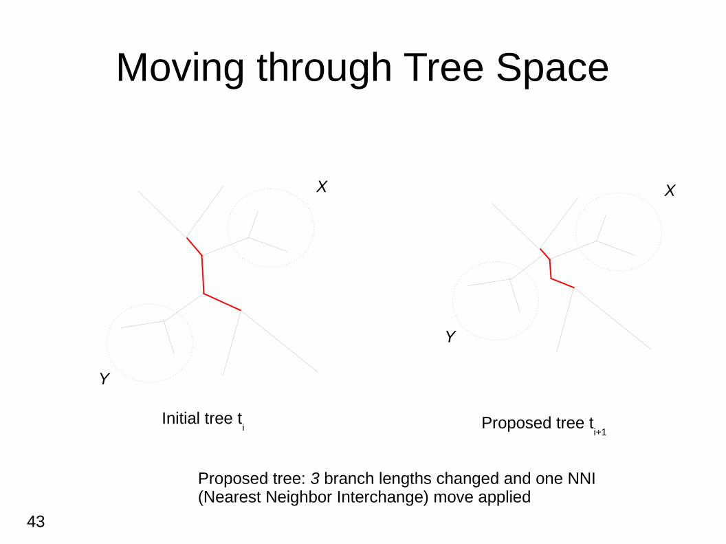
Initial tree ti Proposed tree t
i+1
Proposed tree: 3 branch lengths changed and one NNI (Nearest Neighbor Interchange) move applied
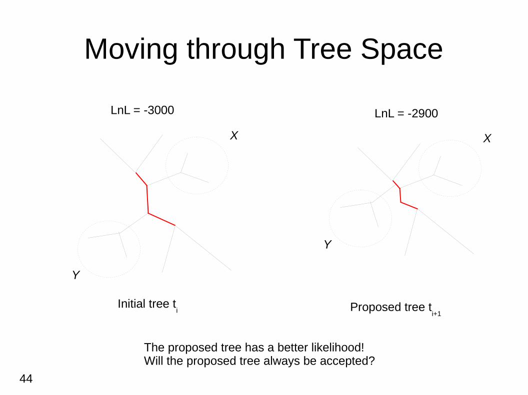
44
Moving through Tree Space
X
Y
X
Y
Initial tree ti Proposed tree t
i+1
The proposed tree has a better likelihood!Will the proposed tree always be accepted?
LnL = -3000 LnL = -2900
45
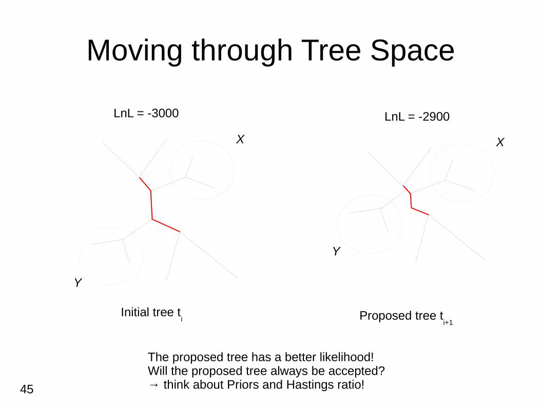
Moving through Tree Space
X
Y
X
Y
Initial tree ti Proposed tree t
i+1
The proposed tree has a better likelihood!Will the proposed tree always be accepted?→ think about Priors and Hastings ratio!
LnL = -3000 LnL = -2900
46
Outline for today
● Markov-Chain Monte-Carlo methods
● Metropolis-coupled MCMC-methods
● Some phylogenetic MCMC proposals
● Reversible jump MCMC
47
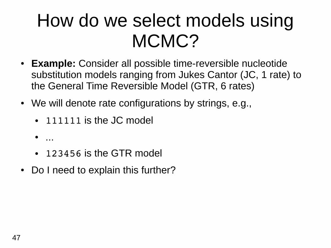
How do we select models using MCMC?
● Example: Consider all possible time-reversible nucleotide substitution models ranging from Jukes Cantor (JC, 1 rate) to the General Time Reversible Model (GTR, 6 rates)
● We will denote rate configurations by strings, e.g.,
● 111111 is the JC model
● ...
● 123456 is the GTR model
● Do I need to explain this further?
48
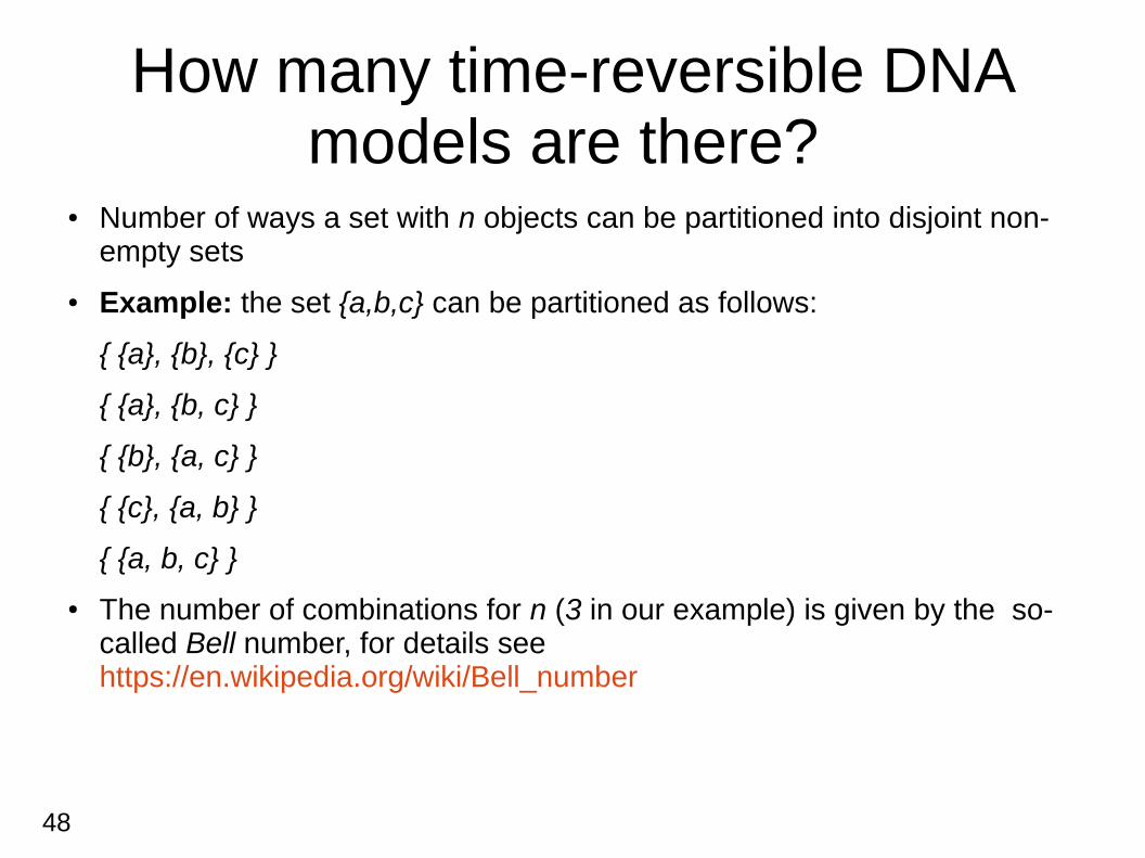
How many time-reversible DNA models are there?
● Number of ways a set with n objects can be partitioned into disjoint non-empty sets
● Example: the set {a,b,c} can be partitioned as follows:
{ {a}, {b}, {c} }
{ {a}, {b, c} }
{ {b}, {a, c} }
{ {c}, {a, b} }
{ {a, b, c} }
● The number of combinations for n (3 in our example) is given by the so-called Bell number, for details see https://en.wikipedia.org/wiki/Bell_number
49
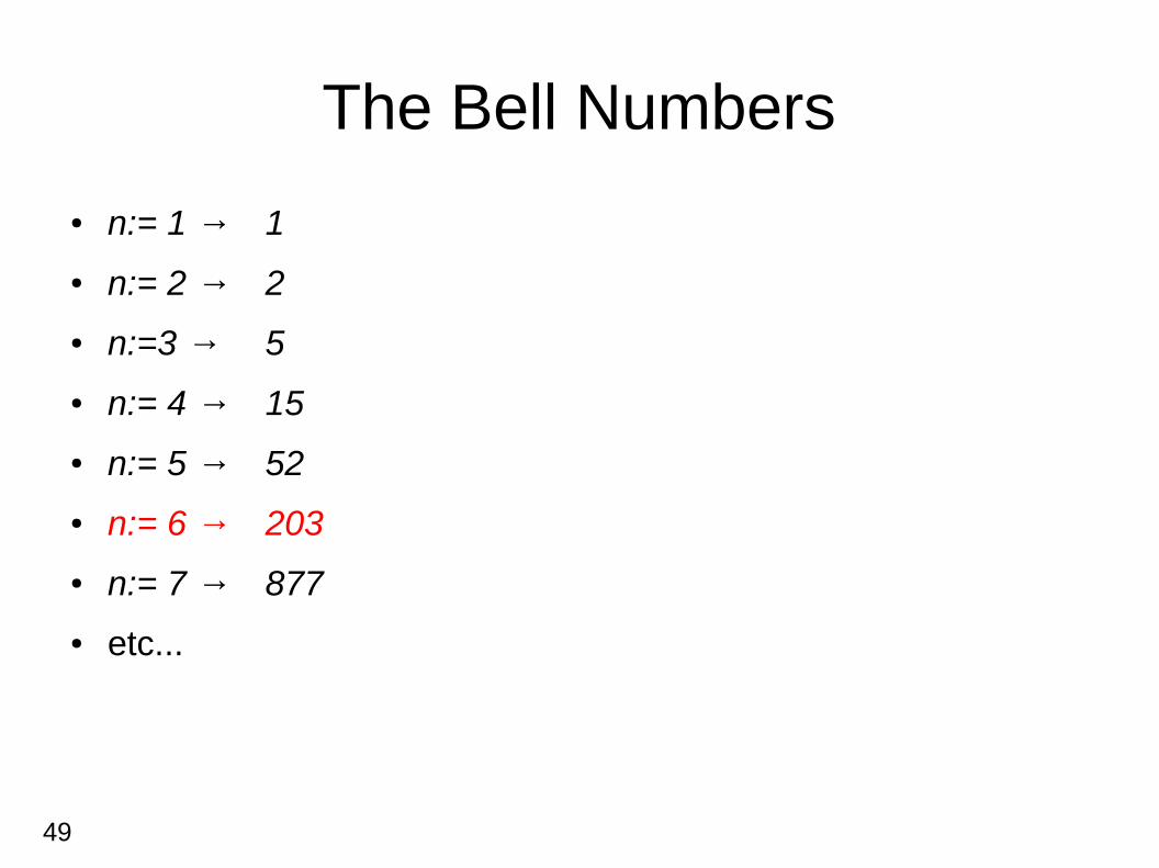
The Bell Numbers
● n:= 1 → 1
● n:= 2 → 2
● n:=3 → 5
● n:= 4 → 15
● n:= 5 → 52
● n:= 6 → 203
● n:= 7 → 877
● etc...
50
What do we need?
● Apart from our usual suspect parameters (tree topology, branch lengths, stationary frequencies, substitution rates, α), we also want to integrate over different models now …
● What are the problems we need to solve?
51
What do we need?
● Apart from our usual suspect parameters (tree topology, branch lengths, stationary frequencies, substitution rates, α), we also want to integrate over different models now …
● What are the problems we need to solve?
● Problem #1: we need to design proposals for moving between different models
● Problem #2: those models have different numbers of parameters, we can not directly compare likelihoods
● Here we use MCMC to not only sample model parameters, but also models

52
Problem #1Model Proposals
● Any ideas?
53
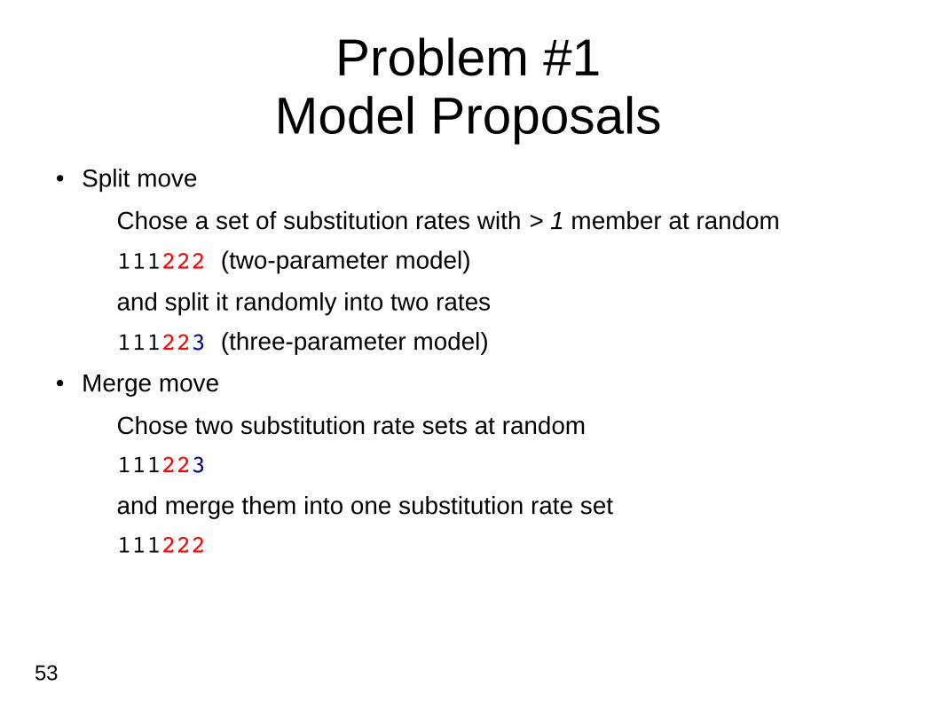
Problem #1Model Proposals
● Split move
Chose a set of substitution rates with > 1 member at random
111222 (two-parameter model)
and split it randomly into two rates
111223 (three-parameter model)
● Merge move
Chose two substitution rate sets at random
111223
and merge them into one substitution rate set
111222
54
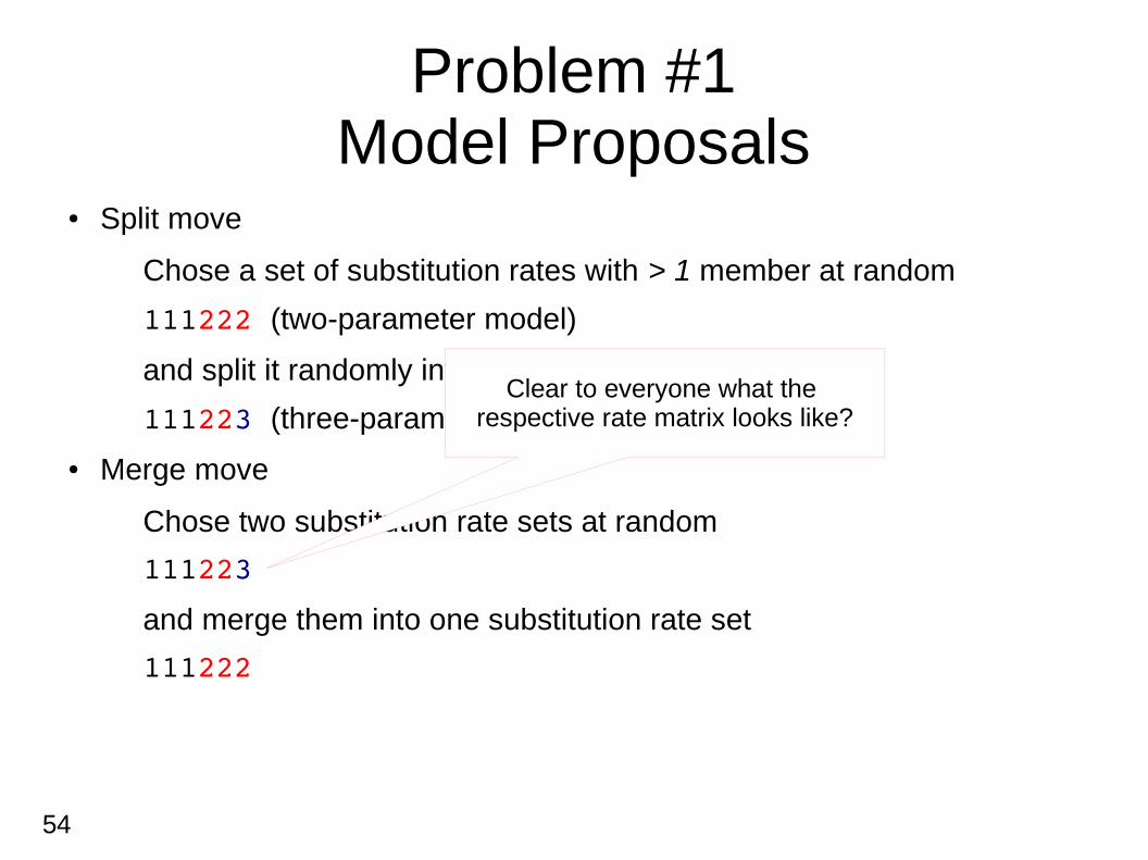
Problem #1Model Proposals
● Split move
Chose a set of substitution rates with > 1 member at random
111222 (two-parameter model)
and split it randomly into two rates
111223 (three-parameter model)
● Merge move
Chose two substitution rate sets at random
111223
and merge them into one substitution rate set
111222
Clear to everyone what the respective rate matrix looks like?
55
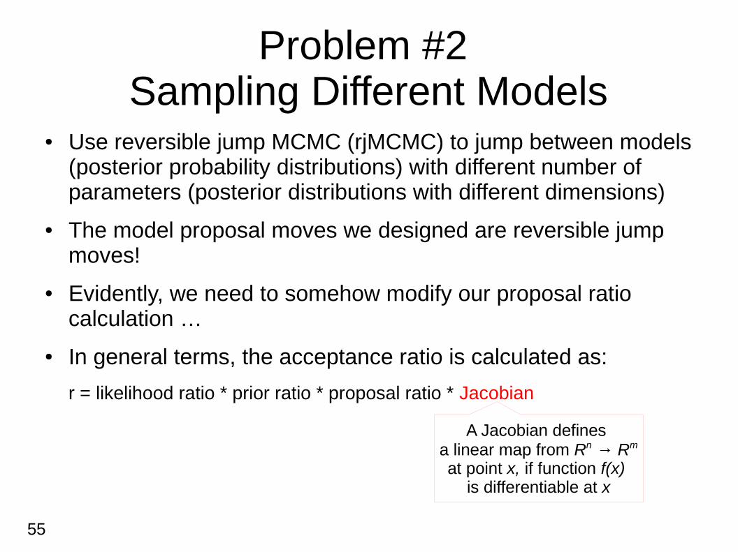
Problem #2 Sampling Different Models
● Use reversible jump MCMC (rjMCMC) to jump between models (posterior probability distributions) with different number of parameters (posterior distributions with different dimensions)
● The model proposal moves we designed are reversible jump moves!
● Evidently, we need to somehow modify our proposal ratio calculation …
● In general terms, the acceptance ratio is calculated as:
r = likelihood ratio * prior ratio * proposal ratio * Jacobian
A Jacobian defines a linear map from Rn → Rm
at point x, if function f(x) is differentiable at x
56
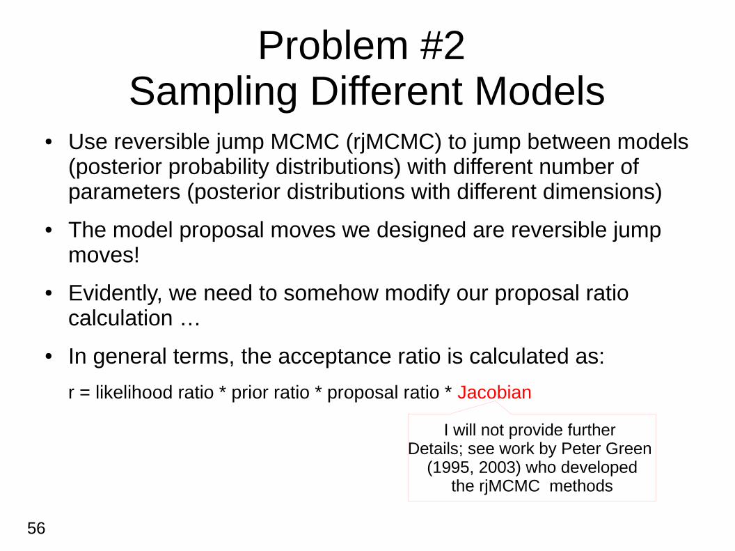
Problem #2 Sampling Different Models
● Use reversible jump MCMC (rjMCMC) to jump between models (posterior probability distributions) with different number of parameters (posterior distributions with different dimensions)
● The model proposal moves we designed are reversible jump moves!
● Evidently, we need to somehow modify our proposal ratio calculation …
● In general terms, the acceptance ratio is calculated as:
r = likelihood ratio * prior ratio * proposal ratio * Jacobian
I will not provide further Details; see work by Peter Green
(1995, 2003) who developedthe rjMCMC methods
57
rjMCMC - summary
● Need to design moves that can jump back and forth between models of different dimensions (parameter counts)
● Need to extend acceptance ratio calculation to account for jumps between different models
● The posterior probability of a specific model (e.g., JC or GTR) is calculated as the fraction of time (fraction of samples) the MCMC chain visited/spent time/generations sampling within that model ...


