Ion Petre and Erik De Vink (Eds.): Third International Workshop onComputational Models for Cell Processes (CompMod 2011)EPTCS 67, 2011, pp. 3–18, doi:10.4204/EPTCS.67.3

Modelling Spatial Interactions in the Arbuscular MycorrhizalSymbiosis using the Calculus of Wrapped Compartments∗

Cristina Calcagno1, Mario Coppo2, Ferruccio Damiani2, Maurizio Drocco2

Eva Sciacca2 , Salvatore Spinella2 and Angelo Troina2

1Dipartimento di Biologia Vegetale, Universita di Torino2Dipartimento di Informatica, Universita di Torino

Arbuscular mycorrhiza (AM) is the most wide-spread plant-fungus symbiosis on earth. Investigatingthis kind of symbiosis is considered one of the most promising ways to develop methods to nurtureplants in more natural manners, avoiding the complex chemical productions used nowadays to pro-duce artificial fertilizers. In previous work we used the Calculus of Wrapped Compartments (CWC)to investigate different phases of the AM symbiosis. In this paper, we continue this line of researchby modelling the colonisation of the plant root cells by the fungal hyphae spreading in the soil. Thisstudy requires the description of some spatial interaction. Although CWC has no explicit featuremodelling a spatial geometry, the compartment labelling feature can be effectively exploited to de-fine a discrete surface topology outlining the relevant sectors which determine the spatial propertiesof the system under consideration. Different situations and interesting spatial properties can be mod-elled and analysed in such a lightweight framework (which has not an explicit notion of geometrywith coordinates and spatial metrics), thus exploiting the existing CWC simulation tool.

1 Introduction

Arbuscular mycorrhiza (AM) is the most wide-spread plant-fungus symbiosis on earth [25]. Investigatingthis kind of symbiosis is considered one of the most promising ways to develop methods to nurture plantsin more natural manners, avoiding the complex chemical productions used nowadays to produce artificialfertilizers.

In previous works [17, 45] in the context of the BioBITS project [11] we investigated different phasesof the AM symbiosis by using the Calculus of Wrapped Compartments (CWC) [19], a variant of theCalculus of Looping Sequences (CLS) [7, 6]. These calculi have been designed to represent in a formalway biological entities such as molecules, DNA strands and cells. Starting from an alphabet of atomicelements (atoms for short) and from an alphabet of labels, CWC terms are defined as multisets of atomsand compartments. A compartment consists of a wrap (a multiset of atoms detailing the elements ofinterest on the membrane), a content (a term) and a type (a label). The evolution of the system is drivenby a set of rewrite rules modelling the reactions of interest (elements interaction and movement). Inprevious work, we have introduced in CWC rules a notion of rate which allow CWC to be equippedwith a semantics given in terms of Continuous Time Markov Chains (CTMCs), thus enabling stochasticsimulation built following the standard Gillespie’s approach [24]. Moreover, we have defined a hybridsimulation algorithm to speed up the simulation procedure while keeping the exactness of Gillespie’smethod, [18]. The simulation tool [2] has been integrated in the FastFlow [4] programming frameworkfor the execution of parallel simulations in multi-core platforms [3].

∗This research is funded by the BioBITs Project (Converging Technologies 2007, area: Biotechnology-ICT), RegionePiemonte.

4 Modelling Spatial Interactions in the AM Symbiosis using CWC

In this paper, we continue our ongoing research on the AM symbiosis by modelling the colonizationof the plant root cells by the fungal hyphae spreading in the soil. The interaction begins with a moleculardialogue between the plant and the fungus. Host roots release signalling molecules characterized asstrigolactones which induce alterations in the fungal physiology and hyphal branching. In response tothe plant signal AM fungi produce a symbiotic signal, the “Myc Factor”. One of the first responseobserved in epidermal plant root cells is a repeated oscillation of Ca2+ concentration preparing to thereorganization of the cell for the fungal penetration. Following this event, fungal hyphae enter andcross the epidermal cells, growing inter-and intracellularly all along the root in order to spread fungalstructures. Once inside the inner layers of the cortical cells, specialised fungal hyphae differentiate intoarbuscules where the nutrients exchange between the two organisms occur.

To represent this kind of behaviour we need to model some spatial properties of the system like themovement of the hyphae in the soil and their penetration and articulation in the root tissue. To this aimwe exploit the fact that the notion of compartment can also be used, in a very natural way, to representspatial regions (with a fixed topology) in which the labels play a key role in defining the spatial properties.These kind of compartments are thus considered as the topological sectors in the analysed model. In thisframework, the movement and growth of system elements are described via specific rules (involvingadjacent compartments) and the functionalities of biological components can be affected by the spatialconstraints given by the sector in which they interact with other elements. A similar approach can befound in [34] where the topological structure of the components is expressed via explicit links whichrequire ad-hoc rules to represent movements of biological entities.

Although our approach does not support an explicit representation of continuous space, we can ex-ploit the topological structure of compartments, their inter-relations, and their relative placement as astarting point to implicitly define spatial properties. This level of abstraction is suitable to model somesituations where it is not needed to explicitly specify the space occupied by the elements of the sys-tem. Avoiding to introduce explicit features for modeling a spatial geometry (e.g., coordinates, position,extension, motion direction and speed, rotation, collision and overlap detection, communication range,etc.) may in some cases reduce the complexity of the models and simplify the analysis of the system andthe simulation procedure.

1.1 Summary

The remainder of the paper is organised as follows. In Section 2 we recall the syntax and semanticsof CWC. In Section 3, through a few chosen paradigmatic examples, we start giving some hint aboutspatial modelling and analysis within the CWC framework. In Section 4 we exploit the approach tomodel some spatial interaction in the Arbuscular Mycorrhizal Symbiosis. In particular, we show howmolecules (carrying the communication signals between the plant and the fungus) diffuse in the soil, andhow the fungus contacts, through its hyphae, the cells of the plant root. Finally, in Section 5 we brieflydiscuss related and possible future work and draw our conclusions.

2 The Calculus of Wrapped Compartments

The Calculus of Wrapped Compartments (CWC) (see [19, 17]) is based on a nested structure of ambi-ents delimited by membranes with specific proprieties. Biological entities like cells, bacteria and theirinteractions can be easily described in CWC.

C. Calcagno, M. Coppo, F. Damiani, M. Drocco, E. Sciacca, S. Spinella and A. Troina 5

(a) (b) (c)

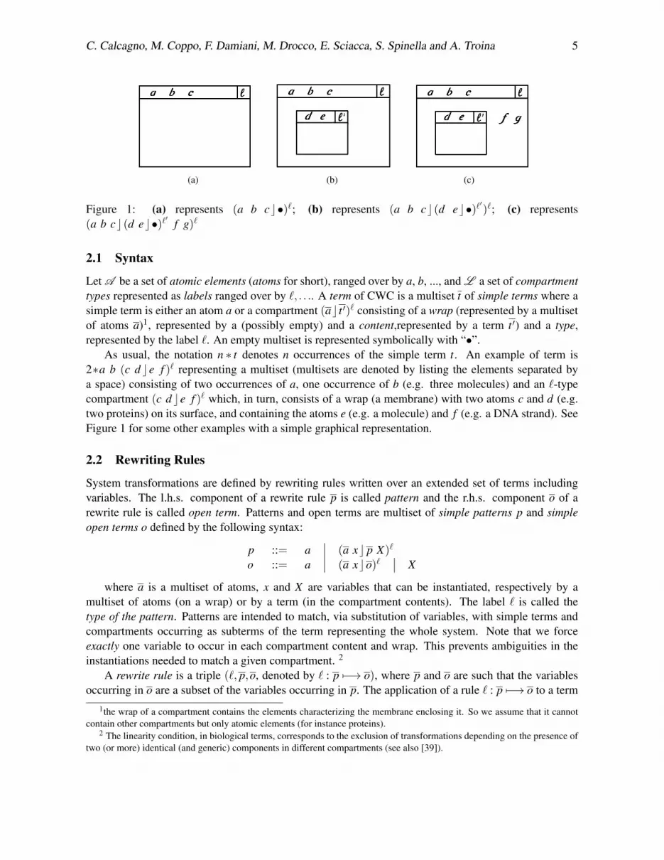
Figure 1: (a) represents (a b cc•)`; (b) represents (a b cc(d ec•)`′)`; (c) represents(a b cc(d ec•)`′ f g)`

2.1 Syntax

Let A be a set of atomic elements (atoms for short), ranged over by a, b, ..., and L a set of compartmenttypes represented as labels ranged over by `, . . .. A term of CWC is a multiset t of simple terms where asimple term is either an atom a or a compartment (ac t ′)` consisting of a wrap (represented by a multisetof atoms a)1, represented by a (possibly empty) and a content,represented by a term t ′) and a type,represented by the label `. An empty multiset is represented symbolically with “•”.

As usual, the notation n ∗ t denotes n occurrences of the simple term t. An example of term is2∗a b (c d ce f )` representing a multiset (multisets are denoted by listing the elements separated bya space) consisting of two occurrences of a, one occurrence of b (e.g. three molecules) and an `-typecompartment (c d ce f )` which, in turn, consists of a wrap (a membrane) with two atoms c and d (e.g.two proteins) on its surface, and containing the atoms e (e.g. a molecule) and f (e.g. a DNA strand). SeeFigure 1 for some other examples with a simple graphical representation.

2.2 Rewriting Rules

System transformations are defined by rewriting rules written over an extended set of terms includingvariables. The l.h.s. component of a rewrite rule p is called pattern and the r.h.s. component o of arewrite rule is called open term. Patterns and open terms are multiset of simple patterns p and simpleopen terms o defined by the following syntax:

p ::= a∣∣ (a xc p X)`

o ::= a∣∣ (a xco)`

∣∣ X

where a is a multiset of atoms, x and X are variables that can be instantiated, respectively by amultiset of atoms (on a wrap) or by a term (in the compartment contents). The label ` is called thetype of the pattern. Patterns are intended to match, via substitution of variables, with simple terms andcompartments occurring as subterms of the term representing the whole system. Note that we forceexactly one variable to occur in each compartment content and wrap. This prevents ambiguities in theinstantiations needed to match a given compartment. 2

A rewrite rule is a triple (`, p,o, denoted by ` : p 7−→ o), where p and o are such that the variablesoccurring in o are a subset of the variables occurring in p. The application of a rule ` : p 7−→ o to a term

1the wrap of a compartment contains the elements characterizing the membrane enclosing it. So we assume that it cannotcontain other compartments but only atomic elements (for instance proteins).

2 The linearity condition, in biological terms, corresponds to the exclusion of transformations depending on the presence oftwo (or more) identical (and generic) components in different compartments (see also [39]).

6 Modelling Spatial Interactions in the AM Symbiosis using CWC

t is performed in the following way: 1) Find in t (if it exists) a compartment of type ` with content uand a substitution σ of variables by ground terms (i.e. terms without occurrences of variables) such thatu = σ(p X), where X is a variable not occurring in p, o; and 2) Replace in t the subterm u with σ(o X).We write t 7−→ t ′ if t ′ is obtained by applying a rewrite rule to t.

For instance, the rewrite rule ` : a b 7−→ c means that in all compartments of type ` containing anoccurrence of a b, it can be replaced by c. While the rewrite rule ` : (xca b X)`1 7−→ (xcc X)`2 meansthat, if contained in a compartment of type `, all compartments of type `1 and containing an a b in theircontent can change their type to `2 and an occurrence of a b can be replaced by c.Remark. For uniformity we assume that the term representing the whole system is always a singlecompartment labelled > with an empty wrap, i.e., all systems are represented by a term of the shape(•c t)>, which we will also write as t for simplicity.

2.3 Stochastic Simulation

A stochastic simulation model for biological systems can be defined along the lines of the one presentedby Gillespie in [24], which is, de facto, the standard way to model quantitative aspects of biologicalsystems. The basic idea of Gillespie’s algorithm is that a rate function is associated with each consideredchemical reaction which is used as the parameter of an exponential distribution modelling the probabilitythat the reaction takes place. In the standard approach this reaction rate is obtained by multiplying thekinetic constant of the reaction by the number of possible combinations of reactants that may occur inthe region in which the reaction takes place, thus modelling the law of mass action. In [19], the reactionrate is defined in a more general way by associating to each reduction rule a function which can alsodefine rates based on different principles as, for instance, the Michaelis-Menten nonlinear kinetics.

In the examples of this paper it is reasonable to assume a linear dependence of the reaction rate onthe number of possible combinations of interacting components, so we will follow the standard approachin defining reaction rates. Each reduction rule is then enriched by the kinetic constant k of the reactionthat it represents (notation ` : p k7−→ o). For instance in evaluating the application rate of the stochasticrewrite rule R = ` : a b X k7−→ c X to the term t = a a b b in a compartment of type ` we must considerthe number of the possible combinations of reactants of the form a b in t. Since each occurrence of a canreact with each occurrence of b, this number is 4. So the application rate of R is k ·4.

2.4 The CWC simulator

The CWC simulator [2] is a tool under development at the Computer science Department of Turin Uni-versity, based on Gillespie’s direct method algorithm [24]. It treats CWC models with different ratingsemantics (law of mass action, Michaelis-Menten kinetics, Hill equation) and it can run independentstochastic simulations over CWC models, featuring deep parallel optimizations for multi-core platformson the top of FastFlow [4]. It also performs online analysis by a modular statistical framework.

3 Topological Interpretations within CWC

In this section we provide some hint about spatial modelling and analysis within the CWC frameworkby means of some paradigmatic examples. For simplicity, we will consider the compartments in oursystem to be well-stirred. Thus, also the compartments representing the spatial sectors of our topologywill consist of well-mixed components. Note that the topological analysis described in the following

C. Calcagno, M. Coppo, F. Damiani, M. Drocco, E. Sciacca, S. Spinella and A. Troina 7

examples could be expressed also with other calculi with compartmentalisation such as, for example,BioAmbients [42], Brane Calculi [14] and Beta-Binders [21].

3.1 Cell Growth and Proliferation: A CWC Grid

Eukaryotic cells reproduce themselves by cell cycle which can be divided in two brief periods: the inter-phase during which the cell grows, accumulating nutrients and duplicating its DNA and the mitosis (M)phase, during which the cell splits itself into two distinct cells, often called “daughter cells”. Interphaseproceeds in three stages, G1, S, and G2. G1 (Gap1) is also called the growth phase, and is marked bysynthesis of various enzymes that are required in S phase, mainly those needed for DNA replication. InS phase (Synthesis) DNA replication occurs. The cell then enters the G2 (Gap2) phase, which lasts untilthe cell enters mitosis. Again, significant biosynthesis occurs during this phase, mainly involving theproduction of microtubules, which are required during the process of mitosis.

Spatial representation of the growth of cell populations could be useful in many situations (in thestudy of bacteria colonies, in developmental biology, and in the analysis of cancer cells proliferation).

Intuitively, we may express cell proliferation by describing a finite space through a CWC grid suchthat on each grid cell we can insert a cell of the growing population under analysis. An k×n grid couldbe modelled in CWC with k ∗n compartment labels modelling the grid cells. A cell may grow in one ofthe adjacent grid cells (with a given scheme of adjacency modelled by the set of rewrite rules).

Intuitively, using the atomic element e to denote an empty grid cell, an empty grid could be modelledby the following CWC term:

Prol Grid= (ce)1,1 . . . (ce)1,n

(ce)2,1 . . . (ce)2,n

. . .(ce)m,1 . . . (ce)m,n

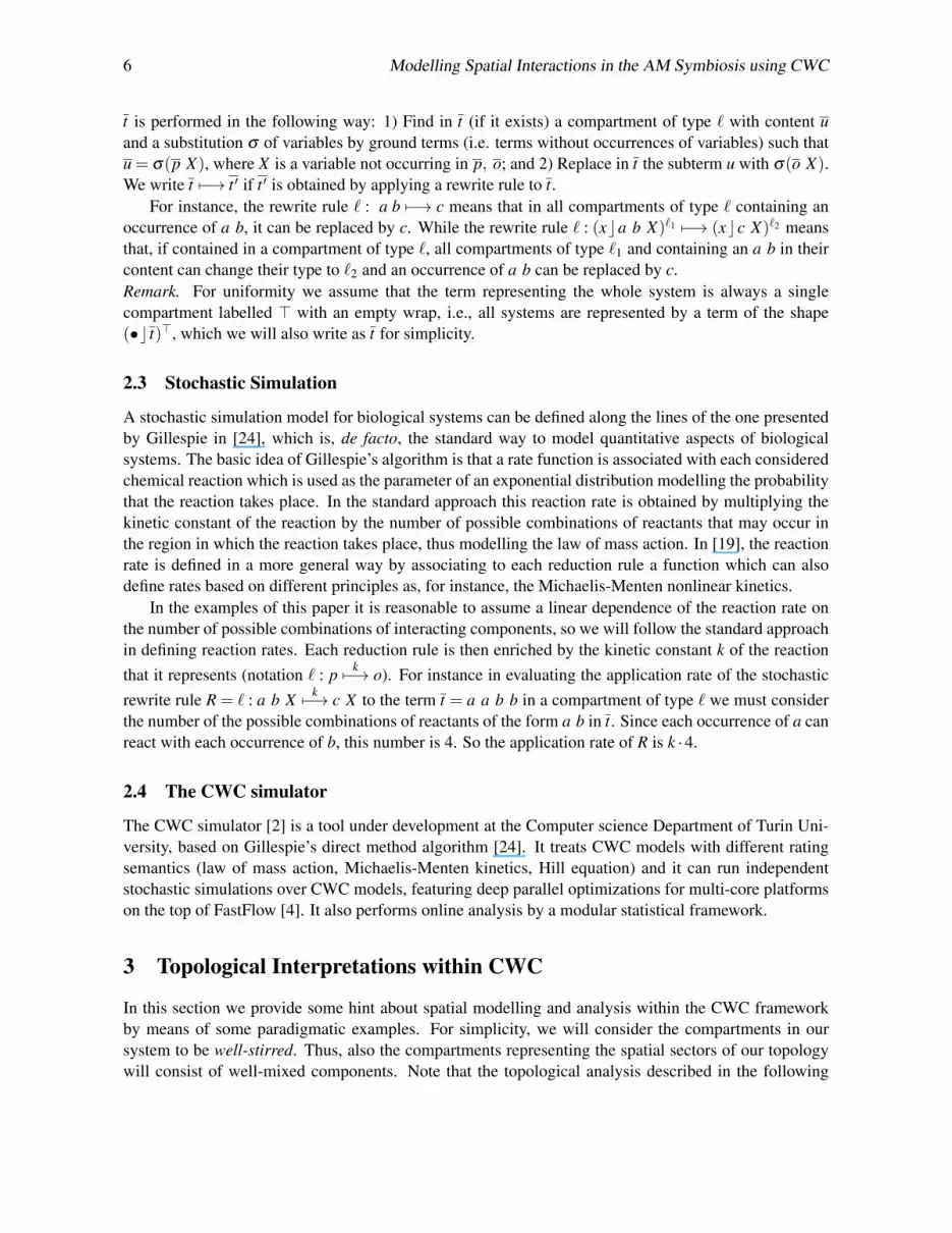
If we represent a cell of our population as a compartment with membrane m and with a single atomin its content representing the phase of the cell cycle (M, G1, S, G2), a grid cell i, j may contain the cell(mcM)cell that could grow, with kinetic kmit , towards the empty grid cell i, j+1 with the rewrite rule 3:

> : (xc(m ycM Y )cell X)i, j(zce Z)i, j+1 kmit7−→ (xc(m ycG1 Y )cell X)i, j(zc(mcG1)cell Z)i, j+1

while cells may change their internal state (cell cycle phase) with the rules:

i, j : (m xcG1 X)cell kphase17−→ (m xcS X)cell

i, j : (m xcS X)cell kphase27−→ (m xcG2 X)cell

i, j : (m xcG2 X)cell kphase37−→ (m xcM X)cell

Note that each element of the grid can be occupied only by one cell, so this model allows only alimited growth of the cells, corresponding to the dimension of the grid. However this could be enough toinvestigate the properties of the cell growth.

3note that under our assumptions the variables will always match only with the empty multiset

8 Modelling Spatial Interactions in the AM Symbiosis using CWC

Figure 2: Quorum Sensing in a distributed topology.

3.2 Quorum Sensing and Molecular Diffusion

Molecular diffusion (or simply diffusion) arises form the motion of particles as a function of temperature,viscosity of the medium and the size (or mass) of the particles. Usually, diffusion explains the flux ofmolecules from a region of higher concentration to one of lower concentration, but it may also occurwhen there is no concentration gradient. The result of the diffusion process is a gradual mixing of theinvolved particles. In the case of uniform diffusion (given a uniform temperature and absent externalforces acting on the particles) the process will eventually result in a complete mixing. Equilibrium isreached when the concentrations of the diffusing molecules between two compartments becomes equal.

Diffusion is of fundamental importance in many disciplines of physics, chemistry, and biology. Inthis subsection we will consider the diffusion of the auto-inducer communication signals in a quorumsensing process where the bacteria initiating the process are distributed in different sectors of an environ-ment (see Figure 2). We consider the sectors of the environment to be connected through channels withdifferent capacities and different speeds regulating the movement of the auto-inducer molecules betweenthe different sectors.

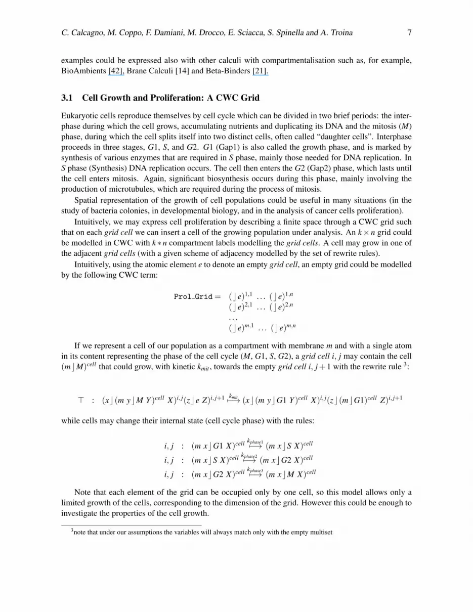
The CWC model describing the system can be found in Appendix A. We modelled the four sectors asfour different compartments with special labels Si allowing the flow of the oxo3 auto-inducer moleculeswith different speed. Bacteria (modelled as compartments with label m) were marked as “active” whenthey reached a sufficient high level of the oxo3 auto-inducer. The results of a simulation running for 30seconds is shown in Figure 3.

Although CWC does not have a direct mechanism to formulate the spatial position of its terms and ametric distance between them, it has the potential to describe topologically different spatial concepts. Forexample, the compartments are able, through the containment specification, to express discrete distanceamong the entities that are inside and those on the outside. Moreover, through the rule kinetics we areable to model space anisotropy (lack of uniformity in all orientations), which are useful to formulatecomplex concepts of reachability. The model discussed in this section is a clear example of these issues.

C. Calcagno, M. Coppo, F. Damiani, M. Drocco, E. Sciacca, S. Spinella and A. Troina 9

Figure 3: Simulation results of oxo3 molecules (left figure) and active bacteria percentage with respectto the total number of bacteria (right figure) in the different sectors.

4 Spatial Interactions in the Arbuscular Mycorrhizal Symbiosis

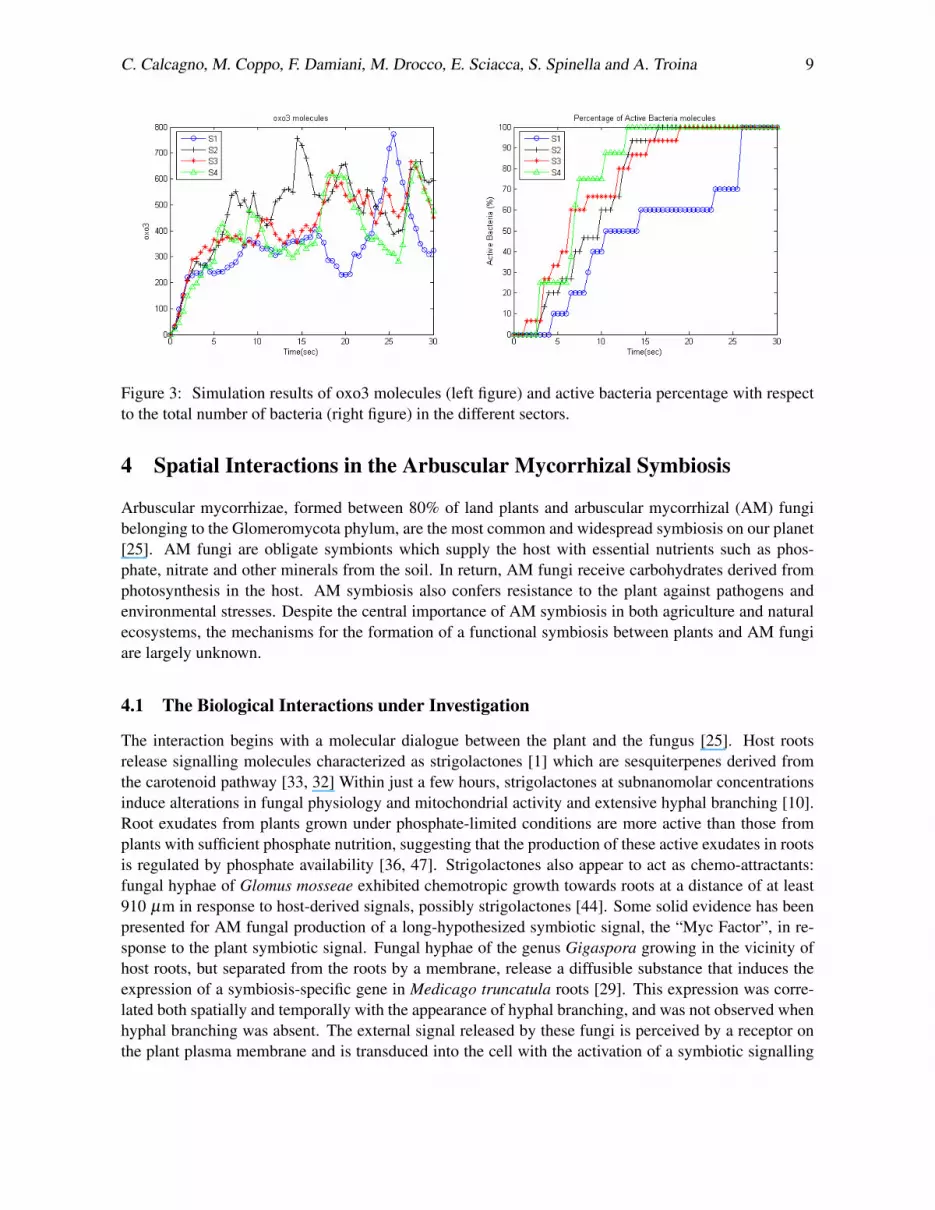
Arbuscular mycorrhizae, formed between 80% of land plants and arbuscular mycorrhizal (AM) fungibelonging to the Glomeromycota phylum, are the most common and widespread symbiosis on our planet[25]. AM fungi are obligate symbionts which supply the host with essential nutrients such as phos-phate, nitrate and other minerals from the soil. In return, AM fungi receive carbohydrates derived fromphotosynthesis in the host. AM symbiosis also confers resistance to the plant against pathogens andenvironmental stresses. Despite the central importance of AM symbiosis in both agriculture and naturalecosystems, the mechanisms for the formation of a functional symbiosis between plants and AM fungiare largely unknown.

4.1 The Biological Interactions under Investigation

The interaction begins with a molecular dialogue between the plant and the fungus [25]. Host rootsrelease signalling molecules characterized as strigolactones [1] which are sesquiterpenes derived fromthe carotenoid pathway [33, 32] Within just a few hours, strigolactones at subnanomolar concentrationsinduce alterations in fungal physiology and mitochondrial activity and extensive hyphal branching [10].Root exudates from plants grown under phosphate-limited conditions are more active than those fromplants with sufficient phosphate nutrition, suggesting that the production of these active exudates in rootsis regulated by phosphate availability [36, 47]. Strigolactones also appear to act as chemo-attractants:fungal hyphae of Glomus mosseae exhibited chemotropic growth towards roots at a distance of at least910 µm in response to host-derived signals, possibly strigolactones [44]. Some solid evidence has beenpresented for AM fungal production of a long-hypothesized symbiotic signal, the “Myc Factor”, in re-sponse to the plant symbiotic signal. Fungal hyphae of the genus Gigaspora growing in the vicinity ofhost roots, but separated from the roots by a membrane, release a diffusible substance that induces theexpression of a symbiosis-specific gene in Medicago truncatula roots [29]. This expression was corre-lated both spatially and temporally with the appearance of hyphal branching, and was not observed whenhyphal branching was absent. The external signal released by these fungi is perceived by a receptor onthe plant plasma membrane and is transduced into the cell with the activation of a symbiotic signalling

10 Modelling Spatial Interactions in the AM Symbiosis using CWC

pathway that lead to the colonization process. One of the first response observed in epidermal cells of theroot is a repeated oscillation of Ca2+ concentration in the nucleus and perinuclear cytoplasm through thealternate activity of Ca2+ channels and transporters [38, 30, 16]. Kosuta and collegues [30] assessed my-corrhizal induced calcium changes in Medicago truncatula plants transformed with the calcium reportercameleon. Calcium oscillations were observed in a number of cells in close proximity to plant/fungalcontact points. Very recently Chabaud and colleagues [16] using root organ cultures of both Medicagotruncatula and Daucus carota observed Ca2+ spiking in AM-responsive zone of the root treated withAM spore exudate.

Once reached the root surface the AM fungus differentiates a hyphopodium via which it enters theroot. A reorganization of the plant cell occurs before the fungal penetration: a thick cytoplasmic bridge(called pre-penetration apparatus -PPA-) is formed and it constitutes a trans-cellular tunnel in which thefungal hypha will grow [23]. Following this event, a hyphal peg is produced which enters and crosses theepidermal cell, avoiding a direct contact between fungal wall and host cytoplasm thanks to a surroundingmembrane of host origin [22]. Than the fungus overcomes the epidermal layer and it grows inter-andintracellularly all along the root in order to spread fungal structures. Once inside the inner layers of thecortical cells the differentiation of specialized, highly branched intracellular hyphae called arbusculesoccur. Arbuscules are considered the major site for nutrients exchange between the two organisms andthey form by repeated dichotomous hyphal branching and grow until they fill the cortical cell. They areephemeral structures [46, 27]: at some point after maturity, the arbuscules collapse, degenerate, and dieand the plant cell regains its previous organization [12]. The mechanisms underlying arbuscule turnoverare unknown but do not involve plant cell death. In arbuscule-containing cells the two partners come inintimate physical contact and adapt their metabolisms to allow reciprocal benefits.

4.2 The CWC Model

We model the Arbuscular Mycorrhyzal symbiosis in a 2D space. The soil environment is partitioned intodifferent concentric layers to account for the distance between the plant root cells and the fungal hyphaewhere the inner layer contains the plant root cells. The plant root tissue is also modelled as concentriclayers each one composed by sectors.

For the sake of simplicity we modelled the soil into 5 different concentric layers (modelled as differ-ent compartments labelled by L0-L4 identifying L4 with the top level>). Although the root has a complexlayered structure we simplified it into 3 concentric layers (one epidermal layer and 2 cortical layers) eachone composed by 5 sectors mapped as different compartments labelled by ei (i = 1 . . .5) for epidermalcells and c jk ( j = 1,2 and k = 1 . . .5) for cortical cells. Exploiting the flexibility of CWC, compartmentlabels are here used to characterize both their spatial position and their biological properties. All thecompartments and the main atoms of the model are depicted in Figure 4.

The stigolactones (atoms S) derived from the carotenoid pathway (atom CP) are released by epidermalcells and can diffuse through the soil degrading their activity when farthest from the plant. This situationwas modelled by the following rules:

(RCPi) L0 : (xcCP X)eiKCP7−→ S(xcCP X)ei i = 1 . . .5

(RSi) Li+1 : (xcS X)LiKS7−→ S(xc X)Li i = 0 . . .3

(RS4) > : SKS7−→ •

(1)

Since phosphate (atoms P) conditions regulate strigolactones biosynthesis inhibiting the carotenoid

C. Calcagno, M. Coppo, F. Damiani, M. Drocco, E. Sciacca, S. Spinella and A. Troina 11

Figure 4: 2D spatial model of the Arbuscular Mycorrhyzal symbiosis.

pathway (atom ICP), the following rules were considered :

(RICPi) L0 : P(xcCP X)eiKICP7−→ P(xc ICP X)ei i = 1 . . .5 (2)

The fungal structure is described by atoms where each atom represents a particular type of fungalcomponent. The atom Spore represents the fungal spore while atoms Hyp represent fungal hyphae. AMfungal hyphae branching towards the plant root is regulated by the strigolacones activity. If we locatethe fungal spore at a fixed distance from the plant root (let us say at the layer Lk where 0 < k < 4) thenthe spore hyphal branching is generated stochastically in the relative inferior and superior layers. In ourexperiments the fungal spore was placed at the soil layer L2. The hyphal branching is radial with respectto the spore position causing a branching away from the spore and promoted at the proximity of the rootby the strigolactones. This branching process was represented by the following rules:

(RF1) L2 : Spore(xc X)L1KF7−→ Spore(xcHyp X)L1

(RF2) L3 : (xcSpore X)L2KF7−→ Hyp(xcSpore X)L2

(RH j) > : (xcHyp X)L3KH7−→ Hyp(xcHyp X)L3

(RH1) L1 : S Hyp(xc X)L0KH17−→ S Hyp(xcHyp X)L0

(3)

The AM fungal production of Myc factor (atom Myc) at the proximity of the root cells inducing thecalcium spiking phenomenon (atom Ca) at a responsive state (atom Resp) which prepares the epidermalcells to include the fungal hyphae was modelled by the following rules:

(RMyc) L0 : Hyp KM7−→Myc Hyp

(RMycCai) L0 : Myc(Resp xc X)eiKMC7−→ (Resp xc Ca X)ei i = 1 . . .5

(RCai) L0 : Hyp(Resp xcCa X)eiKCa7−→ Hyp(NResp xcHyp X)ei i = 1 . . .5

(4)

12 Modelling Spatial Interactions in the AM Symbiosis using CWC

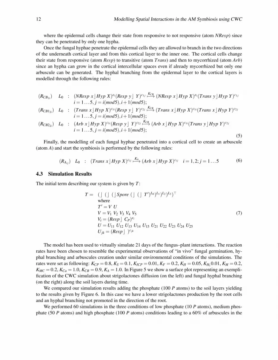
where the epidermal cells change their state from responsive to not responsive (atom NResp) sincethey can be penetrated by only one hypha.

Once the fungal hyphae penetrate the epidermal cells they are allowed to branch in the two directionsof the underneath cortical layer and from this cortical layer to the inner one. The cortical cells changetheir state from responsive (atom Resp) to transitive (atom Trans) and then to mycorrhized (atom Arb)since an hypha can grow in the cortical intercellular spaces even if already mycorrhized but only onearbuscule can be generated. The hyphal branching from the epidermal layer to the cortical layers ismodelled through the following rules:

(RCB1i) L0 : (NResp xcHyp X)ei(Resp yc Y )c1 jKCB7−→ (NResp xcHyp X)ei(Trans ycHyp Y )c1 j

i = 1 . . .5, j = i(mod5), i+1(mod5);

(RCB12i) L0 : (Trans xcHyp X)c1i(Resp yc Y )c2 jKCB7−→ (Trans xcHyp X)c1i(Trans xcHyp Y )c2 j

i = 1 . . .5, j = i(mod5), i+1(mod5);

(RCB22i) L0 : (Arb xcHyp X)c1i(Resp yc Y )c2 jKCB7−→ (Arb xcHyp X)c1i(Trans ycHyp Y )c2 j

i = 1 . . .5, j = i(mod5), i+1(mod5);(5)

Finally, the modelling of each fungal hyphae penetrated into a cortical cell to create an arbuscule(atom A) and start the symbiosis is performed by the following rules:

(RAi j) L0 : (Trans xcHyp X)ci jKA7−→ (Arb xcHyp X)ci j i = 1,2; j = 1 . . .5 (6)

4.3 Simulation Results

The initial term describing our system is given by T :

T = (c (c (cSpore (c (c T ′)L0)L1)L2)L3)>

whereT ′ =V UV =V1 V2 V3 V4 V5Vi = (Respc CP)

ei

U =U11 U12 U13 U14 U15 U21 U22 U23 U24 U25U jk = (Respc )c jk

(7)

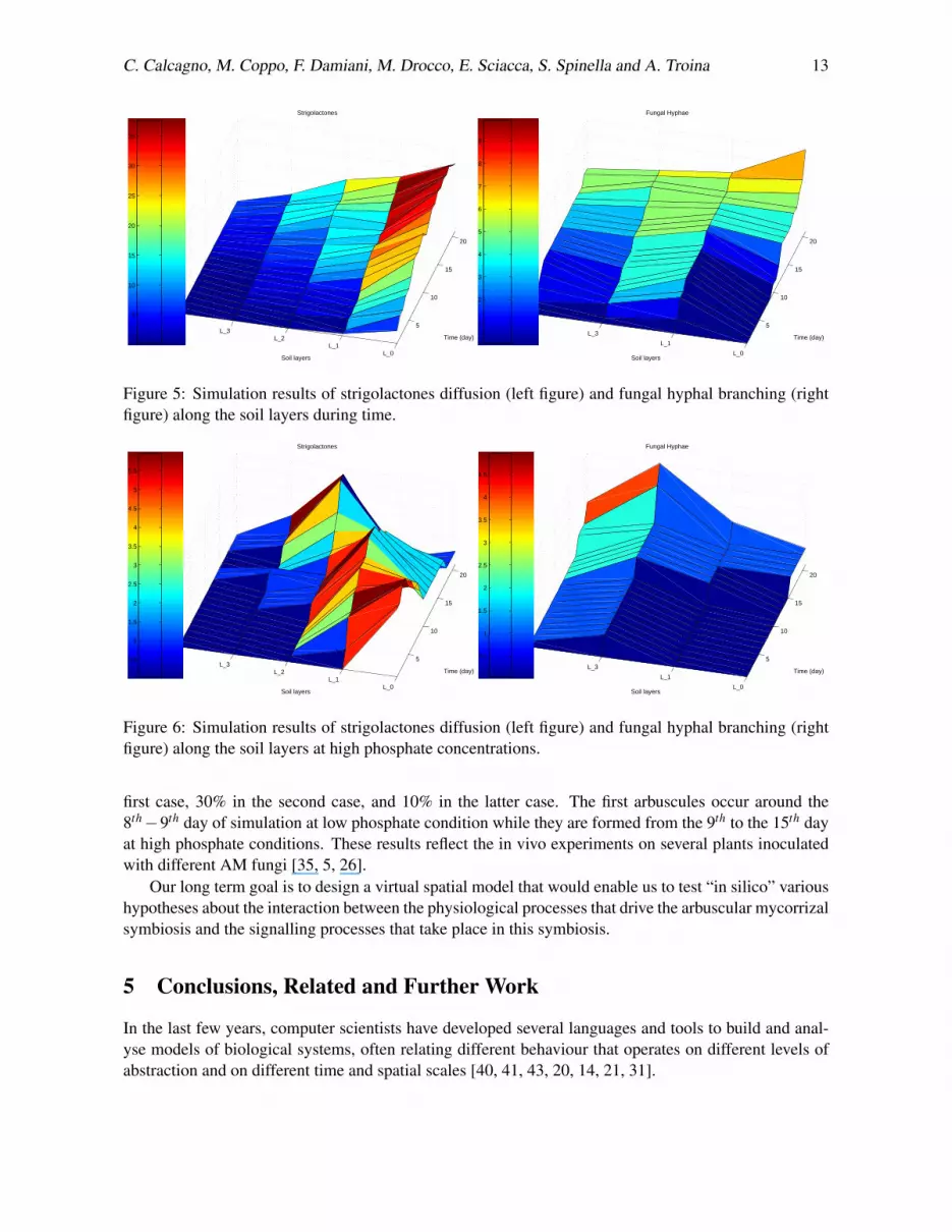
The model has been used to virtually simulate 21 days of the fungus–plant interactions. The reactionrates have been chosen to resemble the experimental observations of “in vivo” fungal germination, hy-phal branching and arbuscules creation under similar environmental conditions of the simulations. Therates were set as following: KCP = 0.8, KS = 0.1, KICP = 0.01, KF = 0.2, KH = 0.05, KH10.01, KM = 0.2,KMC = 0.2, KCa = 1.0, KCB = 0.9, KA = 1.0. In Figure 5 we show a surface plot representing an exempli-fication of the CWC simulation about strigolactones diffusion (on the left) and fungal hyphal branching(on the right) along the soil layers during time.

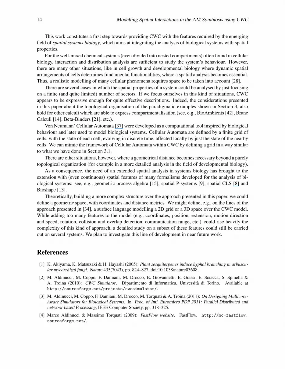
We compared our simulation results adding the phosphate (100 P atoms) to the soil layers yieldingto the results given by Figure 6. In this case we have a lower strigolactones production by the root cellsand an hyphal branching not promoted in the direction of the root.

We performed 60 simulations in the three conditions of low phosphate (10 P atoms), medium phos-phate (50 P atoms) and high phosphate (100 P atoms) conditions leading to a 60% of arbuscules in the

C. Calcagno, M. Coppo, F. Damiani, M. Drocco, E. Sciacca, S. Spinella and A. Troina 13

5

10

15

20

L_0L_1

L_2L_3

L_4

0

10

20

30

40

Time (day)

Strigolactones

Soil layers

5

10

15

20

25

30

35

5

10

15

20

L_0

L_1

L_3

L_4

0

2

4

6

8

10

Time (day)

Fungal Hyphae

Soil layers

1

2

3

4

5

6

7

8

9

Figure 5: Simulation results of strigolactones diffusion (left figure) and fungal hyphal branching (rightfigure) along the soil layers during time.

5

10

15

20

L_0L_1

L_2L_3

L_4

0

1

2

3

4

5

6

Time (day)

Strigolactones

Soil layers

0.5

1

1.5

2

2.5

3

3.5

4

4.5

5

5.5

5

10

15

20

L_0

L_1

L_3

L_4

0

1

2

3

4

5

Time (day)

Fungal Hyphae

Soil layers

0.5

1

1.5

2

2.5

3

3.5

4

4.5

Figure 6: Simulation results of strigolactones diffusion (left figure) and fungal hyphal branching (rightfigure) along the soil layers at high phosphate concentrations.

first case, 30% in the second case, and 10% in the latter case. The first arbuscules occur around the8th−9th day of simulation at low phosphate condition while they are formed from the 9th to the 15th dayat high phosphate conditions. These results reflect the in vivo experiments on several plants inoculatedwith different AM fungi [35, 5, 26].

Our long term goal is to design a virtual spatial model that would enable us to test “in silico” varioushypotheses about the interaction between the physiological processes that drive the arbuscular mycorrizalsymbiosis and the signalling processes that take place in this symbiosis.

5 Conclusions, Related and Further Work

In the last few years, computer scientists have developed several languages and tools to build and anal-yse models of biological systems, often relating different behaviour that operates on different levels ofabstraction and on different time and spatial scales [40, 41, 43, 20, 14, 21, 31].

14 Modelling Spatial Interactions in the AM Symbiosis using CWC

This work constitutes a first step towards providing CWC with the features required by the emergingfield of spatial systems biology, which aims at integrating the analysis of biological systems with spatialproperties.

For the well-mixed chemical systems (even divided into nested compartments) often found in cellularbiology, interaction and distribution analysis are sufficient to study the system’s behaviour. However,there are many other situations, like in cell growth and developmental biology where dynamic spatialarrangements of cells determines fundamental functionalities, where a spatial analysis becomes essential.Thus, a realistic modelling of many cellular phenomena requires space to be taken into account [28].

There are several cases in which the spatial properties of a system could be analysed by just focusingon a finite (and quite limited) number of sectors. If we focus ourselves in this kind of situations, CWCappears to be expressive enough for quite effective descriptions. Indeed, the considerations presentedin this paper about the topological organisation of the paradigmatic examples shown in Section 3, alsohold for other calculi which are able to express compartmentalisation (see, e.g., BioAmbients [42], BraneCalculi [14], Beta-Binders [21], etc.).

Von Neumann’ Cellular Automata [37] were developed as a computational tool inspired by biologicalbehaviour and later used to model biological systems. Cellular Automata are defined by a finite grid ofcells, with the state of each cell, evolving in discrete time, affected locally by just the state of the nearbycells. We can mimic the framework of Cellular Automata within CWC by defining a grid in a way similarto what we have done in Section 3.1.

There are other situations, however, where a geometrical distance becomes necessary beyond a purelytopological organization (for example in a more detailed analysis in the field of developmental biology).

As a consequence, the need of an extended spatial analysis in systems biology has brought to theextension with (even continuous) spatial features of many formalisms developed for the analysis of bi-ological systems: see, e.g., geometric process algebra [15], spatial P-systems [9], spatial CLS [8] andBioshape [13].

Theoretically, building a more complex structure over the approach presented in this paper, we coulddefine a geometric space, with coordinates and distance metrics. We might define, e.g., on the lines of theapproach presented in [34], a surface language modelling a 2D grid or a 3D space over the CWC model.While adding too many features to the model (e.g., coordinates, position, extension, motion directionand speed, rotation, collision and overlap detection, communication range, etc.) could rise heavily thecomplexity of this kind of approach, a detailed study on a subset of these features could still be carriedout on several systems. We plan to investigate this line of development in near future work.

References

[1] K. Akiyama, K. Matsuzaki & H. Hayashi (2005): Plant sesquiterpenes induce hyphal branching in arbuscu-lar mycorrhizal fungi. Nature 435(7043), pp. 824–827, doi:10.1038/nature03608.

[2] M. Aldinucci, M. Coppo, F. Damiani, M. Drocco, E. Giovannetti, E. Grassi, E. Sciacca, S. Spinella &A. Troina (2010): CWC Simulator. Dipartimento di Informatica, Universita di Torino. Available athttp://sourceforge.net/projects/cwcsimulator/.

[3] M. Aldinucci, M. Coppo, F. Damiani, M. Drocco, M. Torquati & A. Troina (2011): On Designing Multicore-Aware Simulators for Biological Systems. In: Proc. of Intl. Euromicro PDP 2011: Parallel Distributed andnetwork-based Processing, IEEE Computer Society, pp. 318–325.

[4] Marco Aldinucci & Massimo Torquati (2009): FastFlow website. FastFlow. http://mc-fastflow.

sourceforge.net/.

C. Calcagno, M. Coppo, F. Damiani, M. Drocco, E. Sciacca, S. Spinella and A. Troina 15

[5] S. Asimi, V. Gianinazzi-Pearson & S. Gianinazzi (1980): Influence of increasing soil phosphorus levels oninteractions between vesicular-arbuscular mycorrhizae and Rhizobium in soybeans. Canadian Journal ofBotany 58(20), pp. 2200–2205, doi:10.1139/b80-253.

[6] R. Barbuti, A. Maggiolo-Schettini, P. Milazzo, P. Tiberi & A. Troina (2008): Stochastic Calculus of LoopingSequences for the Modelling and Simulation of Cellular Pathways. Transactions on Computational SystemsBiology IX, pp. 86–113.

[7] R. Barbuti, A. Maggiolo-Schettini, P. Milazzo & A. Troina (2006): A Calculus of Looping Sequences forModelling Microbiological Systems. Fundam. Inform. 72(1-3), pp. 21–35.

[8] Roberto Barbuti, Andrea Maggiolo-Schettini, Paolo Milazzo & Giovanni Pardini (2009): Spatial Calculus ofLooping Sequences. Electr. Notes Theor. Comput. Sci. 229(1), pp. 21–39, doi:10.1016/j.entcs.2009.02.003.

[9] Roberto Barbuti, Andrea Maggiolo-Schettini, Paolo Milazzo, Giovanni Pardini & Luca Tesei (2011): SpatialP systems. Natural Computing 10(1), pp. 3–16, doi:10.1007/s11047-010-9187-z.

[10] A. Besserer, V. Puech-Pages, P. Kiefer, V. Gomez-Roldan, A. Jauneau, S. Roy, J.C. Portais, C. Roux,G. Becard & N. Sejalon-Delmas (2006): Strigolactones stimulate arbuscular mycorrhizal fungi by activatingmitochondria. PLoS Biology 4(7), pp. 1239–1247, doi:10.1371/journal.pbio.0040226.

[11] BioBITs website. http://www.biobits.di.unipmn.it/.

[12] P. Bonfante-Fasolo (1984): Anatomy and morphology of VA mycorrhizae. VA mycorrhiza .

[13] Federico Buti, Diletta Cacciagrano, Flavio Corradini, Emanuela Merelli & Luca Tesei (2010): BioShape: aspatial shape-based scale-independent simulation environment for biological systems. Procedia CS 1(1), pp.827–835, doi:10.1016/j.procs.2010.04.090.

[14] L. Cardelli (2004): Brane Calculi. In: Proc. of CMSB’04, LNCS 3082, Springer, pp. 257–278.

[15] Luca Cardelli & Philippa Gardner (2010): Processes in Space. In: Proc. of the 6th international conferenceon Computability in Europe, CiE’10, Springer-Verlag, pp. 78–87.

[16] M. Chabaud, A. Genre, B.J. Sieberer, A. Faccio, J. Fournier, M. Novero, D.G. Barker & P. Bonfante (2011):Arbuscular mycorrhizal hyphopodia and germinated spore exudates trigger Ca2+ spiking in the legume andnonlegume root epidermis. New Phytologist doi:10.1111/j.1469-8137.2010.03464.x.

[17] M. Coppo, F. Damiani, M. Drocco, E. Grassi, M. Guether & A. Troina (2011): Modelling Ammonium Trans-porters in Arbuscular Mycorrhiza Symbiosis. Transactions on Computational Systems Biology XIII, pp.85–109.

[18] Mario Coppo, Ferruccio Damiani, Maurizio Drocco, Elena Grassi, Eva Sciacca, Salvatore Spinella &Angelo Troina (2010): Hybrid Calculus of Wrapped Compartments. In: 4th International Meeting onMembrane Computing and Biologically Inspired Process Calculi (MeCBIC’10), 40, EPTCS, pp. 102–120,doi:10.4204/EPTCS.40.8.

[19] Mario Coppo, Ferruccio Damiani, Maurizio Drocco, Elena Grassi & Angelo Troina (2010): Stochastic Cal-culus of Wrapped Compartments. In: 8th Workshop on Quantitative Aspects of Programming Languages(QAPL’10), 28, EPTCS, pp. 82–98, doi:10.4204/EPTCS.28.6.

[20] V. Danos & C. Laneve (2004): Formal molecular biology. Theor. Comput. Sci. 325(1), pp. 69–110,doi:10.1016/j.tcs.2004.03.065.

[21] P. Degano, D. Prandi, C. Priami & P. Quaglia (2006): Beta-binders for Biological Quantitative Experiments.Electr. Notes Theor. Comput. Sci. 164(3), pp. 101–117, doi:10.1016/j.entcs.2006.07.014.

[22] A. Genre & P. Bonfante (2007): Check-in procedures for plant cell entry by biotrophic microbes. MolecularPlant-Microbe Interactions 20(9), pp. 1023–1030, doi:10.1094/MPMI-20-9-1023.

[23] A. Genre, M. Chabaud, T. Timmers, P. Bonfante & D.G. Barker (2005): Arbuscular mycorrhizal fungi elicita novel intracellular apparatus in Medicago truncatula root epidermal cells before infection. The Plant CellOnline 17(12), p. 3489, doi:10.1105/tpc.105.035410.

[24] D. Gillespie (1977): Exact stochastic simulation of coupled chemical reactions. J. Phys. Chem. 81, pp.2340–2361, doi:10.1021/j100540a008.

16 Modelling Spatial Interactions in the AM Symbiosis using CWC

[25] M.J. Harrison (2005): Signaling in the arbuscular mycorrhizal symbiosis. Annu. Rev. Microbiol. 59, pp.19–42, doi:10.1146/annurev.micro.58.030603.123749.

[26] C.M. Hepper (1983): The effect of nitrate and phosphate on the vesicular-arbuscular mycorrhizal infectionof lettuce. New Phytologist 93(3), pp. 389–399, doi:10.1111/j.1469-8137.1983.tb03439.x.

[27] H. Javot, R.V. Penmetsa, N. Terzaghi, D.R. Cook & M.J. Harrison (2007): A Medicago truncatula phosphatetransporter indispensable for the arbuscular mycorrhizal symbiosis. Proceedings of the National Academyof Sciences 104(5), p. 1720, doi:10.1073/pnas.0608136104.

[28] B. Kholodenko (2006): Cell-signalling dynamics in time and space. Nature Reviews Molecular Cell Biology7, pp. 165–176, doi:10.1038/nrm1838.

[29] S. Kosuta, M. Chabaud, G. Lougnon, C. Gough, J. Denarie, D.G. Barker & G. Becard (2003): A Dif-fusible Factor from Arbuscular Mycorrhizal Fungi Induces Symbiosis-Specific MtENOD11 Expression inRoots ofMedicago truncatula. Plant Physiology 131(3), p. 952, doi:10.1104/pp.011882.

[30] S. Kosuta, S. Hazledine, J. Sun, H. Miwa, R.J. Morris, J.A. Downie & G.E.D. Oldroyd (2008): Differentialand chaotic calcium signatures in the symbiosis signaling pathway of legumes. Proceedings of the NationalAcademy of Sciences 105(28), p. 9823, doi:10.1073/pnas.0803499105.

[31] J. Krivine, R. Milner & A. Troina (2008): Stochastic Bigraphs. Electron. Notes Theor. Comput. Sci. 218, pp.73–96, doi:10.1016/j.entcs.2008.10.006.

[32] J.A. Lopez-Raez, T. Charnikhova, V. Gomez-Roldan, R. Matusova, W. Kohlen, R. De Vos, F. Verstappen,V. Puech-Pages, G. Becard, P. Mulder et al. (2008): Tomato strigolactones are derived from carotenoidsand their biosynthesis is promoted by phosphate starvation. New Phytologist 178(4), pp. 863–874,doi:10.1111/j.1469-8137.2008.02406.x.

[33] R. Matusova, K. Rani, F.W.A. Verstappen, M.C.R. Franssen, M.H. Beale & H.J. Bouwmeester (2005): Thestrigolactone germination stimulants of the plant-parasitic Striga and Orobanche spp. are derived from thecarotenoid pathway. Plant Physiology 139(2), p. 920, doi:10.1104/pp.105.061382.

[34] Sara Montagna & Mirko Viroli (2010): A Framework for Modelling and Simulating Networks of Cells. Electr.Notes Theor. Comput. Sci. 268, pp. 115–129, doi:10.1016/j.entcs.2010.12.009.

[35] B. Mosse (1973): Advances in the study of vesicular-arbuscular mycorrhiza. Annual Review of Phytopathol-ogy 11(1), pp. 171–196, doi:10.1146/annurev.py.11.090173.001131.

[36] G. Nagahashi & D.D. Douds Jr (2000): Partial separation of root exudate components and their effectsupon the growth of germinated spores of AM fungi. Mycological Research 104(12), pp. 1453–1464,doi:10.1017/S0953756200002860.

[37] John Von Neumann (1966): Theory of Self-Reproducing Automata. University of Illinois Press, Champaign,IL, USA.

[38] G.E.D. Oldroyd & J.A. Downie (2008): Coordinating nodule morphogenesis with rhizobial infection inlegumes. Annu. Rev. Plant Biol. 59, pp. 519–546, doi:10.1146/annurev.arplant.59.032607.092839.

[39] Nicolas Oury & Gordon Plotkin (2011): Multi-Level Modelling via Stochastic Multi-Level Multiset Rewrit-ing. Draft submitted to MSCS.

[40] C. Priami, A. Regev, E. Y. Shapiro & W. Silverman (2001): Application of a stochastic name-passingcalculus to representation and simulation of molecular processes. Inf. Process. Lett. 80(1), pp. 25–31,doi:10.1016/S0020-0190(01)00214-9.

[41] G. Paun (2002): Membrane computing. An introduction. Springer.

[42] A. Regev, E. M. Panina, W. Silverman, L. Cardelli & E. Y. Shapiro (2004): BioAmbients: an abstraction forbiological compartments. Theor. Comput. Sci. 325(1), pp. 141–167, doi:10.1016/j.tcs.2004.03.061.

[43] A. Regev & E. Shapiro (2002): Cells as computation. Nature 419, p. 343, doi:10.1007/3-540-36481-1 1.

[44] C. Sbrana & M. Giovannetti (2005): Chemotropism in the arbuscular mycorrhizal fungus Glomus mosseae.Mycorrhiza 15(7), pp. 539–545, doi:10.1007/s00572-005-0362-5.

C. Calcagno, M. Coppo, F. Damiani, M. Drocco, E. Sciacca, S. Spinella and A. Troina 17

[45] E Sciacca, S Spinella, A Genre & C Calcagno (2011): Analysis of Calcium Spiking in Plant Root Epidermisthrough CWC Modeling. In: CS2BIO11, pp. 1–12.

[46] R. Toth & R.M. Miller (1984): Dynamics of arbuscule development and degeneration in a Zea mays mycor-rhiza. American journal of botany 71(4), pp. 449–460, doi:10.2307/2443320.

[47] K. Yoneyama, Y. Takeuchi & T. Yokota (2001): Production of clover broomrape seed germination stimulantsby red clover root requires nitrate but is inhibited by phosphate and ammonium. Physiologia Plantarum112(1), pp. 25–30, doi:10.1034/j.1399-3054.2001.1120104.x.

Appendix A: Quorum Sensing and Molecular Diffusion Model

Pseudomonas aeruginosa uses quorum sensing to keep low the expression of virulence factors until thecolony has reached a certain density, when an autoinduced production of virulence factors is started. Thebacterium membrane, denoted as m, contains only a DNA strand. The DNA is modelled as a sequence ofgenes lasO lasR lasI (atom LasORI), where lasO represents the target to which a complex autoinducer/R-protein binds to promote transcription. The following rewrite rules model the system behaviour (thekinetics are taken from [6]):

(R1) m : LasORI 207−→ LasORI LasR (R2) m : LasORI 57−→ LasORI LasI

(R3) m : LasI 87−→ LasI oxo3 (R4) m : oxo3 LasR 0.257−→ R3

(R5) m : R3 4007−→ oxo3 LasR (R6) m : R3 LasORI 0.257−→ RO3

(R7) m : RO3 107−→ R3 LasORI (R8) m : RO3 12007−→ RO3 LasR

(R9) m : RO3 3007−→ RO3 LasI (R10) m : LasI 17−→ •(R11) m : LasR 17−→ • (R12) m : oxo3 17−→ •(R13) m : I oxo3 0.17−→ A oxo3

(8)

Rules R1 and R2 describe the production from the DNA of proteins LasR and LasI, respectively. RuleR3 describes the production of the autoinducer, modelled as atom oxo3, performed by the LasI enzyme.Rules R4 and R5 describe the complexation and decomplexation of the autoinducer and the LasR protein,where the complex is denoted R3. Rules R7, R8, R9 describe the binding of the activated autoinducer(the RO3 complex) to the DNA and its influence in the production of LasR and LasI. Finally, rulesR10, R11, R12 describe the degradation of proteins. In particular, rule R12 models the degradation of theautoinducer, which can happen both inside and outside the bacterium. Bacteria are marked as “active”(atom A) when reaching a sufficient high level of auto-inducer inside the respective sector otherwise theyare marked as “inactive” (atom I).

The following rules describe the ability of the autoinducer to cross the membrane, in both directionsinside the sectors (different kinetics are used to model the different bandwidths of the channels). Anautoinducer inside the bacterium is modelled as a non-positional element, while autoinducers outsidehave an associated spatial sector Si for i = 1, . . . ,4:

Si : (xcoxo3 X)m 307−→ oxo3(xcX)m

Si : oxo3(xcX)m 17−→ (xcoxo3 X)m

Si : oxo3 17−→ •(9)

18 Modelling Spatial Interactions in the AM Symbiosis using CWC

i\ j 1 2 3 41 ND 0.0 0.0 0.12 0.0 ND 0.2 0.33 0.0 0.2 ND 0.34 0.1 0.3 0.3 ND

Table 1: Values for the kinetic rates ki j

The diffusion of the autoinducer across the different sectors is described by the following rules:

> : (xcoxo3 X)Si(ycY )S jki j7−→ (xcX)Si(ycoxo3 Y )S j (10)

where ki j is related to the sectors channel capacities. In our experiments the values of ki j are shownin Table 1 where ki j = k ji.

The simulations were carried out using the following initial term T (see Figure 2):

T1 = (c 10∗ (c I LasORI)m)S1 T2 = (c 15∗ (c I LasORI)m)S2

T3 = (c 15∗ (c I LasORI)m)S3 T4 = (c 8∗ (c I LasORI)m)S4

T = T1 T2 T3 T4

(11)

The model above can be easily enriched by adding rules describing also the movement of the bacteriabetween the different sectors and bacteria replication.