JOURNAL OF GEOPHYSICAL RESEARCH, VOL. 103, NO. B12, PAGES 30,183-30,204, DECEMBER 10, 1998

Phase gradient approach to stacking interferograms

David T. Sandwell and Evelyn J. Price Institute of Geophysics and Planetary Physics, Scripps Institution of Oceanography, La Jolla, California

Abstract. The phase gradient approach is used to construct averages and differences of interferograms without phase unwrapping. Our objectives for change detection are to increase fringe clarity and decrease errors due to tropospheric and ionospheric delay by averaging many interferograms. The standard approach requires phase unwrapping, scaling the phase according to the ratio of the perpendicular baseline, and finally forming the average or difference; however, unique phase unwrapping is usually not possible. Since the phase gradient due to topography is proportional to the perpendicular baseline, phase unwrapping is unnecessary prior to averaging or differencing. Phase unwrapping may be needed to interpret the results, but it is delayed until all of the largest topographic signals are removed. We demonstrate the method by averaging and differencing six interferograms having a suite of perpendicular baselines ranging from 18 to 406 m. Cross-spectral analysis of the difference between two Tandem interferograms provides estimates of spatial resolution, which are used to design prestack filters. A wide range of perpendicular baselines provides the best topographic recovery in terms of accuracy and coverage. Outside of mountainous areas the topography has a relative accuracy of better than 2 m. Residual interferograms (single interferogram minus stack) have tilts across the unwrapped phase that are typically 50 mm in both range and azimuth, reflecting both orbit error and atmospheric delay. Smaller-scale waves with amplitudes of 15 mm are interpreted as atmospheric lee waves. A few Global Positioning System (GPS) control points within a frame could increase the precision to -20 mm for a single interferogram; further improvements may be achieved by stacking residual interferograms.

1. Introduction

Synthetic Aperture Radar Interferometry (InSAR) is a promising new too! for making precise geodetic measurements over large areas [Gabriel et al., 1989; Massonnet and Rabaute, 1993; Massonnet et al., 1993; Zebker et al., 1994a; Massonnet and Feigl, 1995a; Dixon et al., 1993; Meade and Sandwell, 1996]. Sums of interferograms could be used to generate high-resolution topographic maps [Zebker and Goldstein, 1986; Werner et al., 1992; Madsen et al., 1993; Zebker et al., 1994b, 1997], while differences may reveal tectonic deformations and atmospheric-ionospheric distur- bances [Afraimovich et al., 1992; Massonnet et al, 1995; Massonnet and Feigl, 1995b; Peltzer et al., 1996; Peltzer and Rosen, 1995; Goldstein, 1995; Rosen et al., 1996; Tarayre and Massonnet, 1996; Zebker et al., 1997]. We present a new approach to the analysis of interferograms based on the gradi- ent of the phase rather than the phase itself. Because this method is largely untested, we attempt to address the following questions: What is the best mathematical model for relating phase and phase gradients given uncertainties in the data? What are the main limitations of InSAR measurements

derived from ERS data for both line of sight (LOS) accuracy and horizontal resolution? How can InSAR data be improved for both topographic recovery and change detection? What is the best design for an InSAR processing system in order to achieve near optimal results and be efficient? Of course, many

Copyright 1998 by the American Geophysical Union.

Paper number 1998JB900008. 0 ! 48-0227/98/! 998 JB900008509.00

of these questions have been adequately addressed in previous publications, and there already exist tested and efficient InSAR codes. Nevertheless, we hope our answers will help clarify the literature in several areas.

Repeat-pass interferometry records the phase difference, modulo 2r•, between the reference and repeat SAR passes. Since the absolute phase difference is not measured, the fundamental quantity in the interferogram is the local phase gradient; phase differences between two points within the frame are best established by contour integration along a con- tinuous path. Assuming there are no true phase discontinuities or layover, the sum of the phase changes around any closed loop within the interferogram must be zero (i.e., zero residue) [Goldstein et al., 1988' Ghiglia and Pritt, 1998], so phase changes can be described by a conservative (or analytic) function [Resnick and Halliday, 1966, p. 153' Kaplan, 1973, p. 593]. The most important aspects of the phase gradient are that the phase gradient due to topography scales with the perpendicular baseline (equation (A5) and that phase gradient is usually a continuous function of x (range) and y (azimuth), while the wrapped phase contains many 2r• jumps. Because of these properties, phase gradients can be scaled and summed without phase unwrapping, which is notoriously difficult when the signal-to-noise ratio (SNR) is low or when there are phase discontinuities due to layover, shadowing, or displacement at faults [Goldstein et al., 1988' Zebker et al., 1994a]. The conservation property of phase also leads to a theoretically simple two-dimensional phase unwrapping method [Ghiglia and Romero, 1994], which we will employ to remove residues from the stacked phase gradients.

After developing the mathematical framework for the phase

30,183

30,184 SANDWELL AND PRICE: STACKING INTERFEROGRAMS

mission to demonstrate the stacking method and to estimate error sources. On the basis of previous studies, error is divided into short-wavelength radar noise [Li and Goldstein, 1990; Zebker and Villasenor, 1992; Gatelli at al., 1994], intermediate-wavelength tropospheric-ionospheric delay [Goldstein, 1995; Rosen et al., 1996; Massonnet et al., 1994; Tarayre and Massonnet, 1996; Zebker et al., 1997], and longer-wavelength orbit error [Massonnet and Rabute, 1993; Zebker et al., 1994a]. The common signal is the average (stack) of N interferograms, while the noise is the difference between two interferograms or the difference between a single interferogram and the stack. Over the short-wavelength band 0• < 2 km), cross-spectral analysis is used to examine the SNR as a function of wavelength in both the range and azimuthal directions. These estimates are used to design prestack and poststack low-pass filters to suppress short-wavelength noise. Over the intermediate-wavelength band (2-60 km), one SAR image displays tropospheric delays due to atmospheric gravity waves. We use this information on atmospheric delay to better understand the role of ancillary measurements (e.g., Global Positioning System (GPS)) in mitigating these effects. Finally, large-scale differences in interferograms reveal the combined effects of orbit error and average tropospheric- ionospheric delay.

Using this theory and ERS signal characteristics, we are developing an InSAR-processing system. Our design goals are to minimize the complexity of the code and processing steps in order to avoid blunders, to document the system and make it easy to use, to construct a modular system where the main communication channel is through a standardized file header, and to make the code efficient by programming in the most appropriate language. Finally, we avoid adjusting trends across the interferogram and strive to achieve accurate results by using the best available orbit information [Scharroo et al., 1998] and atmospheric corrections.

2. Theory

2.1. Phase Gradient

There are several advantages to working with the phase gradient instead of the phase: (1) The phase gradient can be computed directly from the real and imaginary components of the interferogram [Werner et al., 1992] without first comput- ing the phase; this is especially important when the noise level approaches n rad per pixel. (2) The Earth-flattening cor- rection is easily expressed in terms of a phase gradient (Appendix A). (3) Phase gradients can be averaged or differ- enced without phase unwrapping, so a digital elevation model (DEM) is not required for change detection. The average of the phase gradient from many repeat interferograms, having dif- ferent baselines, will eventually fill the gaps due to temporal and baseline decorrelation. A long-term average should mini- mize the phase errors due to tropospheric and ionospheric delay and thus provide an accurate base for change detection interferograms [Zebker et al., 1997; Fujiwara et al., 1998]. (4) The gradient of the residual phase is a component of strain that can be computed directly from a numerical model of surface deformation. In a previous study [Price and Sandwell, 1998] we showed that these advantages and simplifications enable one to examine shorter wavelengths in the interferogram where the signal-to-noise ratio may be low. There are several disadvantages to this approach: (1) Phase gradients cannot be

compared directly with geodetic measurements of ground dis- placement, so phase unwrapping is still required. (2) The gra- dient operation enhances the short-wavelength noise, so care- ful low-pass filtering of the full-resolution interferogram is required. (3) The standard residue-tree algorithm for phase unwrapping [Goldstein et al., 1988] cannot be used on stacked phase gradients since every closed path of integration has some small residue.

The standard approach to adding or subtracting wrapped phase requires phase unwrapping, scaling the phase by the ratio of the perpendicular baseline, and finally forming the average [Zebker et al., 1994a; Werner et al., 1996]. Unique phase unwrapping is not always possible because areas of the interferogram may not be coherent owing to high relief or wavelength-scale surface changes between the two observa- tion times [Goldstein, 1995]. Here we avoid phase unwrap- ping or delay it until the final step of the processing. Suppose •Pl and •Ps are wrapped phases of two interferograms having long (1) and short (s) baselines, respectively. Because the phase is wrapped, one cannot scale •ps into •Pl (higher fringe rate) or vice versa. However, one can compute and scale the phase gradient. Using the chain rule, we find that the gradient of the phase •p = tan -1 (I/R) is

RVI = 1VR v•p(x) = (1)

R2+i •

where R(x) and/(x) are the real and imaginary components of the Earth-flattened interferogram (equation (A10)). The interferogram is the product of two registered single look complex (SLC)images C•C2' (asterisk denotes complex conjugation), and we will refer to C• and C2 as the reference and repeat images, respectively. Unlike the wrapped phase, which contains many 2n jumps, the real and imaginary components of the interferogram are usually continuous functions, and thus the gradient can be computed with a convolution operation. Because this is a finite difference of nearby pixels, one must minimize the overall phase gradient prior to computing the derivatives; a large part of the phase gradient is removed during the Earth-flattening operation (Appendix A). The average phase gradient from N interferograms each having a perpendicular baseline bi is

v•p = 1 • I v•Pi (2) N i=l •-i

where v•p is the phase gradient per unit baseline. During averaging, one can weight regions of the individual interferograms according to the local correlation and local topographic gradient to achieve an optimal mix. Our initial approach is to edit phase gradient estimates where the correlation falls below 0.2 or the magnitude of the phase gradient is greater than 1.2 rad per pixel.

Proper weighting of the component interferograms will depend on many factors and will require a more complete analysis than we will provide below using only six' interferograms. However, it is clear that the simple unweighted average (equation (2)) is not correct. Consider the average of one 10-m baseline and five 100-m baseline interferograms; the short-baseline interferogram will dominate the stack yet it could be contaminated by atmospheric artifacts. A more reasonable assumption is that each phase gradient estimate has about the same noise level,

SANDWELL AND PRICE: STACKING INTERFEROGRAMS 30,185

independent of baseline length. should be weighted by the absolute baseline length

N

i=1

In this case, the components

N

• sgn(bi) i=1

N

5; b,t i=1

(3)

It is clear that the cumulative baseline in the denominator of

(3) should be large to achieve maximum noise reduction. Longer baselines will provide better noise reduction, but these estimates will not be reliable in areas of rugged terrain where the phase gradient exceeds 1.2 tad per pixel. Hopefully, the estimates from shorter baselines will fill these gaps. Areas of layover can never be filled, and these data gaps pose a major obstacle to the phase unwrapping scheme outlined in section 2.2. [Zebker and Lu, 1998]. In practice, a suite of baselines will provide the best estimate of V0 .

For change detection one selects a candidate interferogram spanning a deformation event and subtracts the long-term average after multiplying by the perpendicular baseline:

WlPchange = WIp- bWIp (4)

If the perpendicular baseline of the interferogram spanning the event is short, then Ibl is small and errors in the topographic correction will be unimportant. If there are several interferograms spanning the same event, then they can be averaged to improve the SNR. Note that this quantity (equation (4))is the horizontal gradient of the line of sight displacement or an unusual component of strain. This strain component could be computed directly from a model, so phase unwrapping is not required. However, phase unwrapping is required to convert the phase gradient anomaly to total phase for comparisons with other geodetic measurements.

There are three end-member cases for change detection: (1) an event where the phase delay anomaly occurs in a single SAR image (usually atmospheric), (2) an event where the phase delay anomaly is permanent (earthquake), and (3) a secular time variation where the strain rate is uniform. In this

study, we only consider case 1 using real data. One approach to isolating an event using noisy data is

N

V q}atmosphere = i= 1 (5) N

i=1

where V0• is the phase gradient anomaly from (4) and ]5 is the spatial correlation function given in (A15). When the quality of the individual change interferograms is highly variable and/or there is a wide range of perpendicular baselines, it is best to downweight the inferior data. For the permanent change, (5)can also be used although it is not necessary to have a common SAR image in all of the component interferograms' they must simply span the event. Finally, for secular change where a constant strain rate is expected, one could weight each interferogram according to its absolute time span Iml'

• sgn(Ati) V•pi V IPsecular = i= 1 (6)

N

i=I

where VlPsecular is strain rate. It is clear that the cumulative time span in the denominator of (6) should be large to achieve maximum noise reduction.

The main new feature of this approach is that the averaging and differencing of many interferograms for topographic recovery and change detection is all done prior to unwrapping the phase. Moreover, in the case of change detection, removal of the main topographic signal reduces the phase gradient toward zero. Thus, in areas of poor correlation, an initial guess of zero phase gradient will provide a good starting point for any phase unwrapping algorithm.

2.2. Phase Unwrapping and Residue Elimination

As noted in section 1, the main weakness of the phase gradient approach is that the gradients must still be integrated to recover topography and/or displacement. The two main unwrapping approaches summarized recently [Zebker and Lu, 1998; Ghiglia and Pritt, 1998] are the residue-tree algorithm [Goldstein et al., 1988] and the least squares algorithm [Hunt, 1979; Ghiglia and Romero, 1994]. Unfortunately, the residue- tree algorithm cannot be applied to stacked phase gradients because the stack is completely populated with small residues. Consider the integration of the phase gradient around a closed path C containing area A. If the phase •p is a continuous function and has continuous first derivatives, then by Stokes theorem it is equal to the integral of the divergence of the curl over the area:

,axay ayax dx dy (7)

Moreover, if the phase represents a conservative function such as topography, then both integrals are zero for all paths/areas. We have computed the curl of the stacked phase gradient of example data sets (below), and as expected, we find paired residues associated with areas of layover. The unfortunate result is that the residues in other areas are never exactly zero. This is because the range and azimuth phase derivatives are performed independently, edited independently, and then stacked independently; there is no reason that they should be consistent. The implication is that different integration paths between two points will always yield slightly different results, and thus the residue-cut tree algorithm cannot be used. These small residues can be eliminated as described next, but this

involves unwrapping the phase using an approach that is functionally equivalent to the least squares approach of [Hunt, 1979].

Oddly, we derive the so-called least squares approach without using the principle of least squares! We then show that our approach is mathematically different from the least squares approach although it is functionally equivalent. Let u(x) = (&p/c•x, &p/c•y) be the numerical estimates of phase gradient (range, azimuth)as given in (1), (3), or (4). Any vector field can be written as the sum of two vectors as

follows:

u = v0+vxw (8)

where 0 is a scalar potential and • is a vector potential. We aqq•!mo that tho phaqo is a conservative filnoticm, en that tho

30,186 SANDWELL AND PRICE: STACKING INTERFEROGRAMS

rotational part of the vector field must be zero everywhere. However, layover, filtering, and stacking interferograms introduce a rotational component that should be eliminated. This is accomplished by taking the divergence of (8) since V ß V x • -- 0. The phase and phase gradient are now related by the following differential equation:

V.u = V2•p (9)

For a finite region the outward component of the phase gradient should be zero along the boundaries [Ghiglia and Romero, 1994]; VO' n = 0, where n is the outward normal. The two-dimensional Fourier transform of (9)provides an algebraic relationship between the total phase Otot(k) and the measured phase gradient u:

Otot(k) = [•l[ik ß I r2[u• 2rrlk 2 (10)

where k = (I/2, x, I/2,y) and It2[.] and F2-i[.] are the forward and inverse two-dimensional Fourier transforms, respectively.

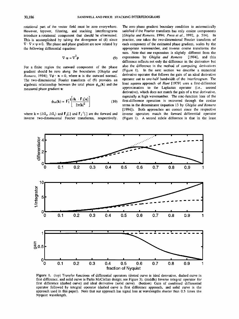
The zero phase gradient boundary condition is automatically satisfied if the Fourier transform has only cosine components [Ghiglia and Romero, 1994; Press et al., 1992, p. 514]. In practice, one takes the two-dimensional Fourier transform of each component of the estimated phase gradient, scales by the appropriate wavenumber, and inverse cosine transforms the sum. Note that our expression is slightly different from the expressions by Ghiglia and Romero [1994], and this difference reflects not only the difference in the derivation but also the difference in the method of computing derivatives (Figure 1). In the next section we describe a numerical derivative operator that follows the gain of an ideal derivative operator out to one-half bandwidth of the interferogram. The least squares approach of Hunt [1979] uses a first-difference approximation to the Laplacian operator (i.e., second derivative), which does not match the gain of a true derivative, especially at high wavenumber. The sinc-function loss of the first-difference operation is recovered through the cosine terms in the denominator (equation 13 by Ghiglia and Romero [1994]). Both approaches are correct since the respective inverse operators match the forward differential operator (Figure 1). A second subtle difference is that in the least

•4

0 0

I I I I I I ,•' i 1

ß '. "" •- 1

0.1 0.2 0.3 0.4 0.5 0.6 0.7 0.8 0.9 1

10

0 0 0.1 0.2 0.3 0.4 0.5 0.6 0.7 0.8 0.9 1

(• 0.5 -

i i i i

0 I I I I I 0 0,1 0,2 0,3 0.4 0.5 0,6 0,7 0.8 0.9

fraction of Nyquist

Figure 1. (top) Transfer functions of differential operators (dotted curve is ideal derivative, dashed curve is first difference, and solid curve is Parks McClellan design; see Figure 3). (middle) Inverse integral operator for first difference (dashed curve) and ideal derivative (solid curve). (bottom) Gain of combined differential operator followed by integral operator (dashed curve is first difference approach, and solid curve is the approach used in this paper). Note that our approach has signal loss at wavelengths shorter than 0.5 times the Nyquist wavelength.

SANDWELL AND PRICE: STACKING INTERFEROGRAMS 30,187

squares approach, two derivatives are performed in the space domain while in our approach one derivative is performed in the space domain while the second is performed in the wavenumber domain. This complicates the computer code slightly because the forward two-dimensional (2-D) transform on each component of phase gradient involves a sine transform (in the differentiated direction) followed by a cosine transform in the other direction.

shaped filter was used to avoid the prominent sidelobes of a simple boxcar average. For ERS-1/2 the spacing of pixels in ground range is -5 times the spacing of pixels in azimuth. We have designed a convolution filter that is nearly isotropic in ground-range and azimuth coordinates:

(11)

3. Data Analysis

3.1. Selection

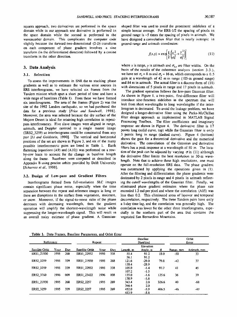
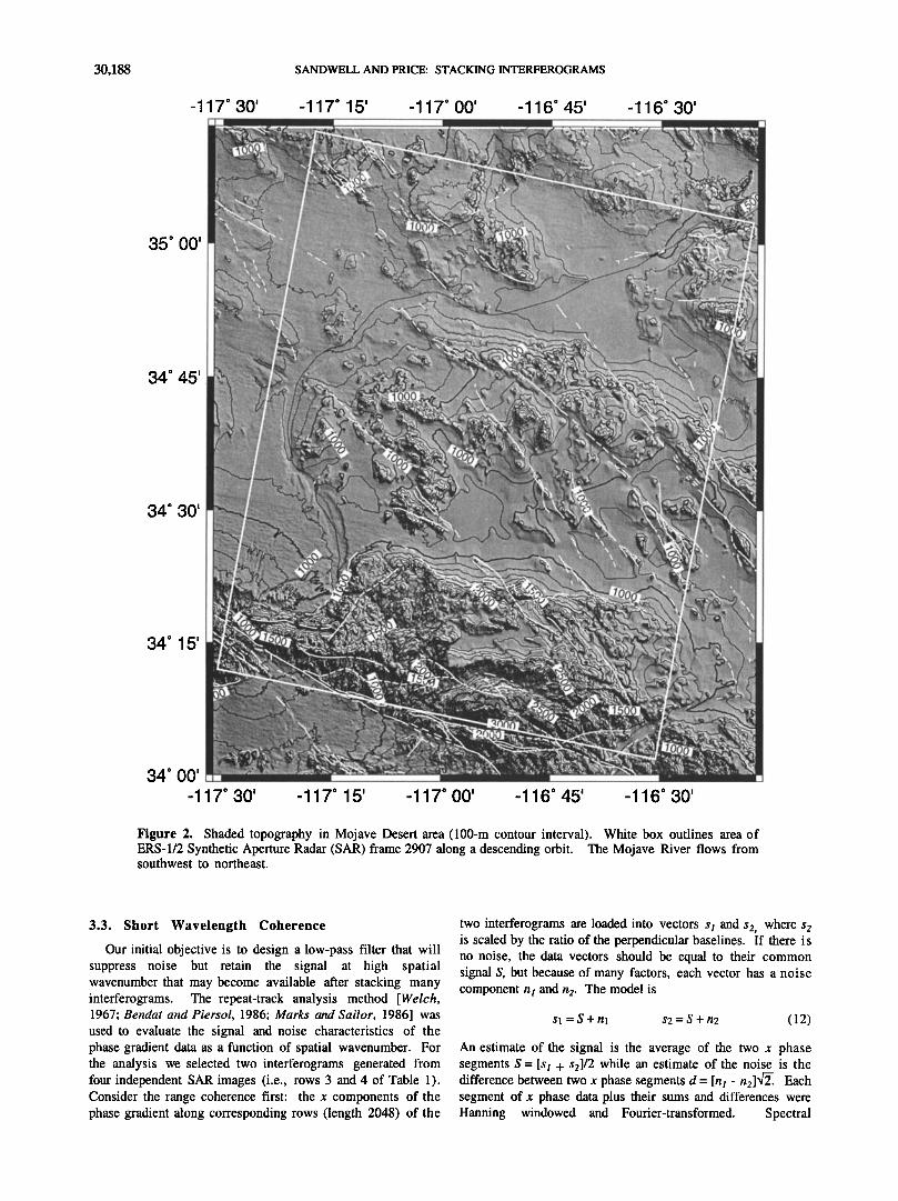
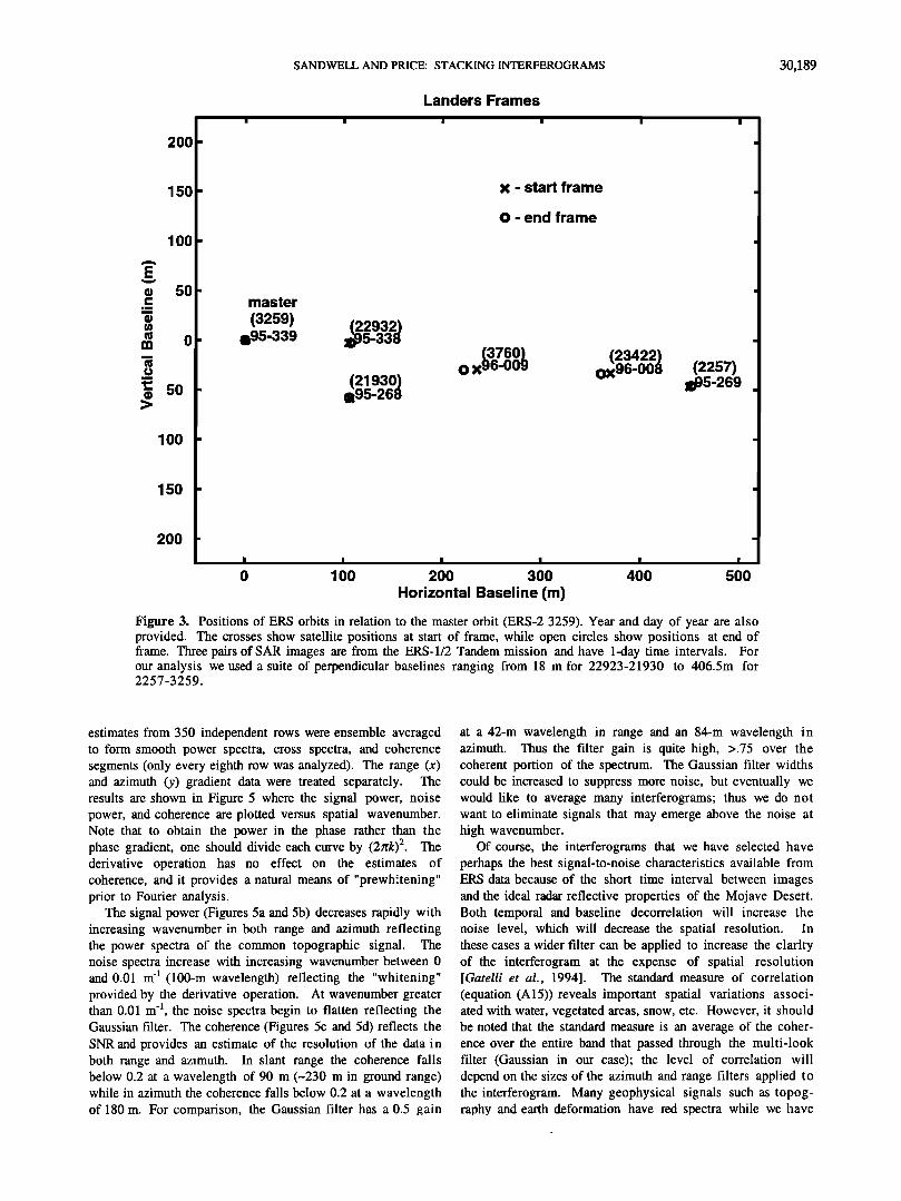
To assess the improvements in SNR due to stacking phase gradients as well as to estimate the various error sources in ERS interferograms, we have selected six frames from the Tandem mission which span a short period of time and have a wide range of baselines (Table 1). From these we have formed six interferograms. The area of the frames (Figure 2) was the site of the 1992 Landers earthquake, so we had purchased the data for a previous study [Price and Sandwell, 1998]. Moreover, the area was selected because the dry surface of the Mojave Desert is ideal for retaining high correlation in repeat- pass interferometry. Five slave images were aligned in range, azimuth, and Doppler centroid to a single master image (ERS2_3259) so interferograms could be constructed from any pair [Li and Goldstein, 1990]. The vertical and horizontal positions of the set are shown in Figure 3, and six of the many possible interferometric pairs are listed in Table 1. Earth flattening (equations (A9) and (A10)) was performed on a row- by-row basis to account for the change in baseline length along the frame. Baselines were computed as described in Appendix B using precise orbits provided by Delft University [Scharroo et al., 1998].

3.2. Design of Low-pass and Gradient Filters

Interferograms formed from full-resolution SLC images contain significant phase noise, especially when the time separation between the repeat and reference images is long or there are disruptions in the surface from vegetation, moisture, or snow. Moreover, if the signal-to-noise ratio of the phase decreases with decreasing wavelength, then the gradient operation will amplify the shortest-wavelength noise while suppressing the longer-wavelength signal. This will result in an overall noisy estimate of phase gradient. A Gaussian-

where x is range, y is azimuth and crx, y are filter widths. On the basis of the results of the coherence analysis (section 3.3.), we have set crx = 8 m and Cry = 16 m, which corresponds to a 0.5 gain at a wavelength of 42 m in range (105-m ground range) and 84 m in azimuth. The actual filter is a discrete form of (11) with dimensions of 5 pixels in range and 17 pixels in azimuth.

The gradient operation follows the low-pass Gaussian filter. As shown in Figure 1, a two-point, first-difference filter will introduce sinc-function sidelobes in the spectrum that will leak from short wavelengths to long wavelengths if the inter- ferogram is decimated. To avoid the leakage problem, we have designed a longer-derivative filter using the Parks-McClellan filter design approach as implemented in MATLAB Signal Processing Toolbox. The filter coefficients and imaginary response are shown in Figure 4. The derivative filter is 17 points long (solid curve, top) while the Gaussian filter is only 5 points long in range (dashed curve). Figure 4 (bottom) shows the gain for a theoretical derivative and the numerical derivative. The convolution of the Gaussian and derivative

filters has a peak response at a wavelength of 50 m. The loca- tion of the peak can be adjusted by varying Cr in (11) although the derivative filter limits the best resolution to 30-m wave-

length. Note that to achieve these high resolutions, one must operate on the full-resolution ERS data. The phase gradient was constructed by applying the operations given in (1). After the filtering and differentiation the phase gradients were decimated by 2 pixels in range and 4 pixels in azimuth reflect- ing the cutoff wavelengths of the Gaussian filter. Finally, we eliminated phase gradient estimates where the phase rate exceeded 1.2 rad per pixel and where the correlation (A15) was less than 0.2. This eliminated areas of layover and temporal decorrelation, respectively. The three Tandem pairs have only a 1-day time lag, and the correlation was generally high. The correlation was lower for the other three interferograms, espe- cially in the southern part of the area that contains the vegetated San Bernardino Mountains.

Table 1. Data Frames, Baseline Parameters, and Orbit Error

Reference Repeat

Satellite Orbit Year Day Satellite Orbit Year Day ERS1_21930 1995 268 ERS1_22932 1995 338

ERS2_3259 1995 339 ERS1_21930 1995 268

ERS2_3259 1995 339 ERS 1_22932 1995 338

ERS2_3760 1996 009 ERS 1_23422 1996 008

ERS1_21930 1995 268 ERS2_2257 1995 269

ERS2_3259 1995 339 ERS2_2257 1995 269

Baseline Orbit Start/End Error

Elevation

Length? m Angle? cz B_ Range 1 mm Azimuth 7 mm 55.4 91.2 18.0 -50 33 56.1 91.2

121.6 -29.0 79.8 -42 37 120.4 -28.9

105.0 -1.4 97.7 41 45 107.2 -1.5

135.0 -1.6 125.6 36 39

138.9 -1.6

343.4 2.0 326.6 40 -68

346.4 2.0

452.0 -5.9 406.5 -46 -49

453.9 -5.8

30,188 SANDWELL AND PRICE: STACKING INTERFEROGRAMS

-117 ø 30' -117 ø 15' -117 ø 00' -116 ø 45' -116 ø 30'

35 ø 00'

34 ø 45'

34 ø 30'

34 ø 15'

34 ø 00' ,. ß -117 ø 30' -117 ø 15' -117 ø 00' -116 ø 45' -116 ø 30'

Figure 2. Shaded topography in Mojave Desert area (100-m contour interval). White box outlines area of ERS-1/2 Synthetic Aperture Radar (SAR) frame 2907 along a descending orbit. The Mojave River flows from southwest to northeast.

3.3. Short Wavelength Coherence

Our initial objective is to design a low-pass filter that will suppress noise but retain the signal at high spatial wavenumber that may become available after stacking many interferograms. The repeat-track analysis method [Welch, 1967; Bendat and Piersol, 1986; Marks and Sailor, 1986] was used to evaluate the signal and noise characteristics of the phase gradient data as a function of spatial wavenumber. For the analysis we selected two interferograms generated from four independent SAR images (i.e., rows 3 and 4 of Table 1). Consider the range coherence first: the x components of the phase gradient along corresponding rows (length 2048) of the

two interferograms are loaded into vectors st and s2, where s2 is scaled by the ratio of the perpendicular baselines. If there i s no noise, the data vectors should be equal to their common signal S, but because of many factors, each vector has a noise component n• and n 2. The model is

sl = S + nl s2 = S + n2 (12)

An estimate of the signal is the average of the two x phase segments S = [s• + s2]/2 while an estimate of the noise is the difference between two x phase segments d = [n• - n2]•. Each segment of x phase data plus their sums and differences were Hanning windowed and Fourier-transformed. Spectral

SANDWELL AND PRICE: STACKING INTERFEROGRAMS 30,189

2OO

150

IO0

5O

0

5O

IO0

150

2OO

master

(3259) •95-339

Landers Frames

! ! i i

(21930) •195-268

x - start frame

0 - end frame

{3760) (23422) 0 x 96'009 0x96-008 (2257)

•B95-269

I , I I I I I

0 100 200 300 400 500

Horizontal Baseline (m)

Figure 3. Positions of ERS orbits in relation to the master orbit (ERS-2 3259). Year and day of year are also provided. The crosses show satellite positions at start of frame, while open circles show positions at end of frame. Three pairs of SAR images are from the ERS-1/2 Tandem mission and have 1-day time intervals. For our analysis we used a suite of perpendicular baselines ranging from 18 m for 22923-21930 to 406.5m for 2257-3259.

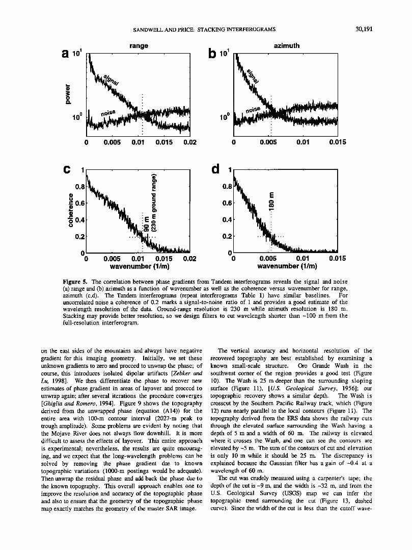
estimates from 350 independent rows were ensemble averaged to form smooth power spectra, cross spectra, and coherence segments (only every eighth row was analyzed). The range (x) and azimuth (y) gradient data were treated separately. The results are shown in Figure 5 where the signal power, noise power, and coherence are plotted versus spatial wavenumber. Note that to obtain the power in the phase rather than the phase gradient, one should divide each curve by (2/rk) 2. The derivative operation has no effect on the estimates of coherence, and it provides a natural means of "prewh"tening" prior to Fourier analysis.

The signal power (Figures 5a and 5b) decreases rapidly with increasing wavenumber in both range and azimuth reflecting the power spectra of the common topographic signal. The noise spectra increase with increasing wavenumber between 0 and 0.01 m 4 (100-m wavelength) reflecting the "whitening" provided by the derivative operation. At wavenumber greater than 0.01 m -1, the noise spectra begin to flatten reflecting the Gaussian filter. The coherence (Figures 5c and 5d) reflects the SNR and provides an estimate of the resolution of the data in both range and azimuth. In slant range the coherence falls below 0.2 at a wavelength of 90 m (-230 m in ground range) while in azimuth the coherence falls below 0.2 at a wavelength of 180 m. For comparison, the Gaussian filter has a 0.5 gain

at a 42-m wavelength in range and an 84-m wavelength in azimuth. Thus the filter gain is quite high, >.75 over the coherent portion of the spectrum. The Gaussian filter widths could be increased to suppress more noise, but eventually We would like to average many interferograms; thus we do not want to eliminate signals that may emerge above the noise at high wavenumber.

Of course, the interferograms that we have selected hav e perhaps the best signal-to-noise characteristics available from ERS data because of the short time interval between images and the ideal radar reflective properties of the Mojave Desert. Both temporal and baseline decorrelation will increase the noise level, which will decrease the spatial resolution. In these cases a wider filter can be applied to increase the clarity of the interferogram at the expense of spatial resolution [Gatelli et al., 1994]. The standard measure of correlation (equation (A15))reveals important spatial variations associ- ated with water, vegetated areas, snow, etc. However, it should be noted that the standard measure is an average of the coher- ence over the entire band that passed through the multi-look filter (Gaussian in our case); the level of correlation will depend on the sizes of the azimuth and range filters applied t o the interferogram. Many geophysical signals such as topog- raphy and earth deformation have red spectra while we have

30,190 SANDWELL AND PRICE: STACKING INTERFEROGRAMS

0.5

0.5

range

60 40 20 0 20 40 60

lag (m)

1.5

0.5

I I I .' I I I ß

ß

_ -

_

-- • • •" • •- 0.01 0.02 0.03 0.04 0.05 0.06

wavenumber (l/m)

Figure 4. (top) Low-pass Gaussian filter (dashed curve) and derivative filter (solid curve) applied to full- resolution interferogram. (bottom) Gain of ideal derivative filter (dotted curve), 17-point convolution filter (solid curve), and Gaussian low-pass filter followed by 17-point derivative filter (dashed curve). The combined filter has little loss for wavelengths greater than 100 m.

shown that the noise spectrum is blue in terms of phase gradi- ent (white in terms of phase).

3.4. Stacking Phase Gradients and Topographic Recovery

Phase gradients from six interferograms were stacked as described by (3). The suite of baselines dramatically increases the dynamic range of ERS phase recovery over all types of terrain. The interferogram with the shortest perpendicular baseline (18 m)has almost complete spatial coverage while coverage of high-relief areas is poor for the longest-baseline interferogram (406 m). The cumulative baseline shown in Figure 6 illustrates the editing associated with layover, high relief, standing water, and agricultural fields. The SAR image ERS1_22932 was shifted by 5600 rows of raw SAR data with respect to its interferometric pair(s); this is reflected in a shaded band along the top of the cumulative baseline image (Figure 6). Out of a possible cumulative baseline of 1054 m (white in Figure 6), there are very few areas having cumulative baseline less than 200 m. Stacked azimuthal and range phase gradients (Figures 7 and 8, respectively) have nearly complete coverage and do not show any discontinuities associated with dropouts from the individual interferograms. One would expect that long-wavelength orbit error would shift each inter-

ferogram to a different average level and that the stack would contain these shifts. However, keep in mind the dramatic suppression of long wavelengths by the derivative filter. For example, a 50-mm orbit error over a 100-km frame will intro- duce a DC offset in phase gradient of only 0.0050 rad per pixel, which is 100 times smaller than typical phase gradients associated with topographyß For an accurate stack it is impor- tant that the cumulative baseline length accurately reflects the baselines of the components used in the stack, especially if the cumulative baseline is short. This is one of the reasons

why accurate orbital information is needed. Since we do not unwrap the phase of the individual interferograms, ground control information cannot be used to estimate the baseline

parameters [e.g., Zebker et al., 1994a]. The stacked range and azimuthal phase gradients were

unwrapped using (10), which relies on complete phase cover- age. From Figure 2 it is clear that this area contains large, long-wavelength components of elevation (phase) change between the low areas of the Mojave River in the north (-600 m)and the high areas of the San Bernardino Mountains (2600 m)on the southeast. In addition, the cumulative baseline in the rugged areas of the San Bernardino Mountains is short and highly variable, making unwrapping the phase difficult. Finally, and most troubling, areas of layover occur

SANDWELL AND PRICE: STACKING INTERFEROGRAMS 30,191

a 101

100

range ß , ,

0 0.005 0.01 0.015 0.02

b10 •

10 o

azimuth , ,

ß

ß

0 0.005 0.01 0.015

C I

0.8

c 0.6

o 0.4

0.2

d I ß ß

0.005 0.01 0.015 0.02

wavenumber (l/m)

0.8

0.6

0.4

0.2

o o o o o.o15

ß .

0.005 0.01

wavenumber (l/m)

Figure 5. The correlation between phase gradients from Tandem interferograms reveals the signal and noise (a) range and (b) azimuth as a function of wavenumber as well as the coherence versus wavenumber for range, azimuth (c,d). The Tandem interferograms (repeat interferograms Table 1) have similar baselines. For uncorrelated noise a coherence of 0.2 marks a signal-to-noise ratio of 1 and provides a good estimate of the wavelength resolution of the data. Ground-range resolution is 230 m while azimuth resolution is 180 m. Stacking may provide better resolution, so we design filters to cut wavelength shorter than -100 m from the full-resolution interferogram.

on the east sides of the mountains and always have negative gradient for this imaging geometry. Initially, we set these unknown gradients to zero and proceed to unwrap the phase' of course, this introduces isolated dipolar artifacts [Zebker and Lu, 1998]. We then differentiate the phase to recover new estimates of phase gradient in areas of layover and proceed to unwrap again; after several iterations the procedure converges [Ghiglia and Romero, 1994]. Figure 9 shows the topography derived from the unwrapped phase (equation (A14)) for the entire area with 100-m contour interval (2027-m peak to trough amplitude). Some problems are evident by noting that the Mojave River does not always flow downhill. It is more difficult to assess the effects of layover. This entire approach is experimental; nevertheless, the results are quite encourag- ing, and we expect that the long-wavelength problems can be solved by removing the phase gradient due to known topographic variations (1000-m postings would be adequate). Then unwrap the residual phase and add back the phase due to the known topography. This overall approach enables one to improve the resolution and accuracy of the topographic phase and also to ensure that the geometry of the topographic phase mat• exactly matches the eeometrv of the master SAR image.

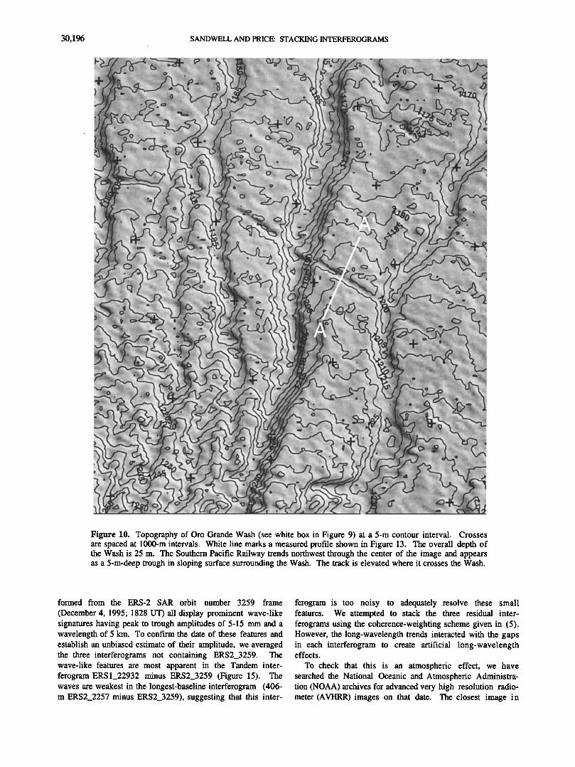
The vertical accuracy and horizontal resolution of the recovered topography are best established by examining a known small-scale structure. Oro Grande Wash in the

southwest comer of the region provides a good test (Figure 10). The Wash is 25 m deeper than the surrounding sloping surface (Figure 11), [U.S. Geological Survey, 1956]; our topographic recovery shows a similar depth. The Wash is crosscut by the Southern Pacific Railway track, which (Figure 12) runs nearly parallel to the local contours (Figure 11). The topography derived from the ERS data shows the railway cuts through the elevated surface surrounding the Wash having a depth of 5 m and a width of 60 m. The railway is elevated where it crosses the Wash, and one can see the contours are

elevated by -5 m. The sum of the contours of cut and elevation is only 10 m while it should be 25 m. The discrepancy is explained because the Gaussian filter has a gain of -0.4 at a wavelength of 60 m.

The cut was crudely measured using a carpenter's tape; the depth of the cut is -9 m, and the width is -32 m, and from the U.S. Geological Survey (USGS) map we can infer the topographic trend surrounding the cut (Figure 13, dashed curve). Since the width of the cut is less than the cutoff wave-

30,192 SANDWELL AND PRICE: STACKING INTERFEROGRAMS

110 -

100 -

0 10 20 30 40 50 60 70 80 90 km

Figure 6. Cumulative baseline (range) shows the sum of the perpendicular baseline estimates that are available for stacking. Maximum baseline of 1050 m is white while zero baseline is black. The shaded patch along the top reflects incomplete data from the 22932 ERS-1 frame. Other shaded areas reflect decorrelation due to vegetation, standing water, and layover. Cumulative baseline is used to normalize the stack (equation (3)) as well as to weight the iterative phase unwrapping for topographic recovery.

length of the low-pass filter, its shape is unimportant, and a Gaussian filter can be applied to the measured profile for comparison with the topography recovered from ERS interferometry (Figure 13, dotted curve). The match is quite good, suggesting that there are no blunders in our processing. Moreover, the 2-m scatter about a straight-line trend suggests that this is the noise level of the relative topographic recovery in this rather flat area.

It is interesting to note that this narrow railway cut has a clearer phase expression than any of the freeways nearby or even the California Aqueduct. Examinations of the backscatter amplitude reveal that railroad tracks are consistently radar bright while nearby roads are radar dark. The brightness is unrelated to the orientation of the track with respect to the radar illumination direction. Why are these tracks so reflec- tive? The answer is that the gravel of the railway bed consists

SANDWELL AND PRICE: STACKING INTERFEROGRAMS 30,193

11o

lOO

9o

8o

7o

6o

50

4o

3o

2o

lO

0 10 20 30 40 km 50 60 70 80 90

Figure 7. Stacked phase gradient in azimuth (black area is -0.15 rad per pixel, and white area is +0.15 rad per pixel) appears as the topography illuminated from the north.

of chunks that are typically >50 mm across. The C band ERS radar has a 56-mm wavelength, so the enhanced reflectivity is due to Bragg scattering from the gravel. The overall width of a gravel railway bed is only 10 m, so even this small area can provide high backscatter. This may have implications for the design of low-cost radar reflectors.

3.5. Orbit Error

The relative orbit error of each interferogram was estimated by computing the difference in phase gradient between the

individual interferogram and the stack as given in (4). The average of the phase gradient difference in range (azimuth) is the slope of the orbit error across (along) the frame. The integral of this slope provides an estimate of orbit error, and these numbers are given in Table 1; errors are typically 40 mm over a distance of 100 km corresponding to a slope error of 0.4 grad. This maps into a perpendicular baseline error (H. Zebker, personal communication, 1996; http://www- ee.stanford.edu/---zebkeff) of-360 mm, which is consistent with, although somewhat larger than, the estimated cross- track orbit error of 300 mm for uncorrelated repeat orbits

30,194 SANDWELL AND PRICE: STACKING INTERFEROGRAMS

11o

lOO

9o

8o

7o

6o

,.•

50

4o

3o

2o

lO

o lO 20 30 40 km SO 60 70 80 90

Figure 8. Stacked phase gradient in range appears as topography illuminated from the west. Note that in rugged areas such as the San Bernardino Mountains in the south, the slope distribution is asymmetric because the radar illuminates the eastern side of the mountains at a steep look angle of 20 ø. This asymmetry, coupled with regions of complete layover, poses a significant problem in phase unwrapping.

[Scharroo et al., 1998]. While we are attributing this slope in the residual interferogram to orbit error, a constant zenith delay will also produce a uniform slope in range [Zebker et al., 1997]. Similarly, a change in zenith delay along the track will mimic a change in parallel baseline component of the orbit error. Thus one cannot distinguish between orbit error and long-wavelength propagation delay. As noted in Table 1, the distance between the reference and repeat orbits changes

monotonically along the frame by up to 4 m. Therefore one must account for these changes in baseline while applying the Earth-flattening correction (equation (A9)).

One of the advantages of the phase gradient approach for change detection is that even long-baseline interferograms can provide accurate change measurements as long as the correlation remains high over the area. The example shown in Figure 14 is a ERS Tandem interferogram (i.e., 1-day time

SANDWELL AND PRICE: STACKING INTERFEROGRAMS 30,195

11o

] . ..i .... i i ,

100

8o

6o

50-

4o

3o

10'

;

10 20 30 40 km $o 60 70 80 90

Figure 9. Unwrapped phase scaled into relief (equation (A14)) and contoured at 100-m intervals. At long wavelengths the cumulative dropouts on the sides of the mountains facing the radar introduce long-wavelength errors in the unwrapped phase. On small scales the relief estimates are quite detailed and accurate.

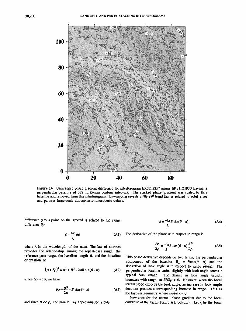
span) having a perpendicular baseline of 326 m (ERS2_2257 minus ERS 1_21930). This unwrapped phase reveals about 70 mm of orbit error and other shorter-wavelength error of --10 ram. There is a wave-like signature at a range of 65 km and an azimuth of 40 km that represents contamination of the stack by atmospheric waves as discussed in section 3.6. Indeed, this contamination introduces large (-30 m) wave-like errors in our estimates of topography (total) phase estimate

above. To reduce these errors, many more interferograms should be averaged (>20).

3.6. Atmospheric Waves

In addition to orbit error, the six change interferograms reveal other phase delays that are presumably due to atmos- pheric and ionospheric effects. The three interferograms

30,196 SANDWELL AND PRICE: STACKING INTERFEROGRAMS

Figure 10. Topography of Oro Grande Wash (see white box in Figure 9) at a 5-m contour interval. Crosses are spaced at 1000-m intervals. White line marks a measured profile shown in Figure 13. The overall depth of the Wash is 25 m. The Southern Pacific Railway trends northwest through the center of the image and appears as a 5-m-deep trough in sloping surface surrounding the Wash. The track is elevated where it crosses the Wash.

formed from the ERS-2 SAR orbit number 3259 frame

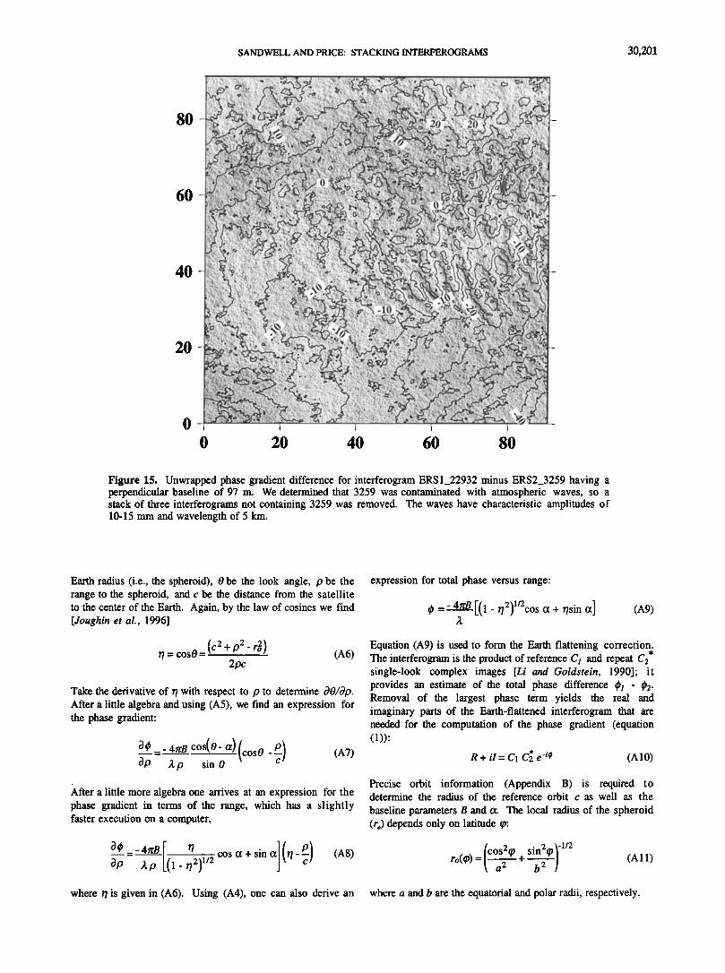
(December 4, 1995; 1828 UT) all display prominent wave-like signatures having peak to trough amplitudes of 5-15 mm and a wavelength of 5 km. To confirm the date of these features and establish an unbiased estimate of their amplitude, we averaged the three interferograms not containing ERS2_3259. The wave-like features are most apparent in the Tandem inter- ferogram ERS1_22932 minus ERS2_3259 (Figure 15). The waves are weakest in the longest-baseline interferogram (406- m ERS2_2257 minus ERS2_3259), suggesting that this inter-

ferogram is too noisy to adequately resolve these small features. We attempted to stack the three residual inter- ferograms using the coherence-weighting scheme given in (5). However, the long-wavelength trends interacted with the gaps in each interferogram to create artificial long-wavelength effects.

To check that this is an atmospheric effect, we have searched the National Oceanic and Atmospheric Administra- tion (NOAA) archives for advanced very high resolution radio- meter (AVHRR)images on that date. The closest image in

SANDWELL AND PRICE: STACKING INTERFEROGRAMS 30,197

Figure 11. Contour map of Oro Grande Wash (USGS, 1956; 20-foot contours) shows intersection with railway cut and fill. This should be compared with the interferometric topographic recovery shown in Figure 10. Profile A-A' is 1000 m long.

time (2045 UT)contains wave-like features in Nevada, although they are not pronounced in the area just north of the San Bernardino. Nevertheless, we believe that the wave-like

features are atmospheric gravity waves on the lee of the San Bernardino Mountains [Holton, 1972, pp. 172-179]. These waves may have moved northeastward during the 2-hour time span between the SAR image and the AVHRR image. Another possibility is that the waves have no visible signature in the AVHRR data. Such features have been seen previously in other interferograms [Tarayre and Massonnet, 1996].

4. Limitations and Unresolved Issues

These initial results suggest that the phase gradient approach will be a good way to treat ERS interferograms when many repeat frames are available. While this report outlines the theory, the applications presented here are quite limited and do not always demonstrate the advantages claimed in the

introduction. To better understand the approach, the following types of research need to be completed:

1. Analyze perhaps >20 repeat images instead of just 6. With only six interferograms one cannot use the stack to begin editing and weeding out the bad estimates. In a similar study, where repeat satellite altimeter profiles were stacked, a high level of confidence was gained when 16 repeats became available, and dramatic improvement was seen when 40 profiles were stacked [Yale et at., 1995].

2. Remove as much known signal as possible before filtering the interferogram; this could be done using a low- resolution digital elevation model [Massonnet et at., 1994]. The expected benefits are a more accurate estimate of correlation [Werner et at., 1996], smaller errors due to numerical differentiation, retention of more high phase rate data in the mountains, and more accurate phase unwrapping especially at long wavelength and near the edges of the area.

3. Further investigate the effects of layover on topographic recovery from stacked phase gradients. Layover is a

30,198 SANDWELL AND PRICE: STACKING INTERFEROGRAMS

Figure 12. Photograph of cut and fill at Oro Grande Wash. (top) looking southeast across Wash with highway 15 in background and (bottom) looking west at railway fill.

particularly difficult problem because it always eliminates data of the same sign; this plagues the Fourier phase unwrapping approach.

4. Design a poststack filter that reflects the noise of the residual interferogram. The coherence analysis shown in Figure 5 suggests that even very noisy interferograms will contain some information at long wavelengths. Perhaps this can be recovered after careful removal of the topographic signature followed by a low-pass filter.

5. Explore a long time series of difference interferograms to isolate the three types of temporal signals (i.e., single event, stepwise event, and secular change).

6. Finally, given that there will always be residual orbit and atmospheric error at the centimeter level and that we would like to observe changes at the millimeter level, one should explore the best approach to using GPS measurements of ground deformation and atmospheric-ionospheric delay to correct the interferograms.

SANDWELL AND PRICE: STACKING INTERFEROGRAMS 30,199

A 6

I

500 400 300 200 1 O0 0 1 O0 200 300 400 500 distance (rn)

Figure 13. Profile A-A' across railway cut. Solid curve is from stacked interferogram, dashed curve is a crude measurement of the cut, and dotted curve is the measured topography convolved with Gaussian filter used to reduce noise in raw interferograms.

5. Summary

We have just scratched the surface on using phase gradients for recovering topography and surface change from SAR interferometry. The theoretical development of the phase gradient and their sums and differences are straightforward. Carefully designed low-pass and gradient filters must be applied to the full-resolution interferogram in order to obtain unbiased estimates of gradient at the shortest possible wavelength. Precise orbits are needed to remove most of the long-wavelength phase gradient as well as to estimate the perpendicular baseline scale factors that are needed for stacking interferograms. In addition, the precise orbits could be used to automate the entire processing sequence, but there is still a problem with the timing accuracy of the ERS data (Appendix B).

Phase unwrapping is still a major problem, which we believe is best solved by first removing all known signals [Massonnet et al., 1996] from the phase maps and then stacking as much data as possible to provide complete 2-D estimates of phase gradient; we still do not know how to deal with areas of layover. The largest component of orbit error appears as a trend across each interferogram, and in theory, just a few GPS control points could be used to correct it. On a smaller scale we show examples of 15 mm of residual

atmospheric delay at a 5-km wavelength. Since the tropospheric perturbations have a red spectrum [Goldstein, 1995], the error is probably larger at longer wavelengths. If this error is stationary in space and in time, then it can be reduced as the square root of the number of individual SAR images used in the stack. Since the primary error sources are concentrated at wavelengths greater than a few kilometers and, as we show, the interferograms can resolve features with wavelengths greater than 200 m, InSAR will provide the most useful information in the 200- to 20,000-m wavelength band. It would be nice to have several years of repeat images to gain some confidence in the overall approach

Appendix A

A1. Phase Gradient Due to Earth Curvature

Here we follow the derivation of Rosen et al. [1996] and

Joughin et al. [1996] to highlight the relationship between phase gradient in range and the topography of the curved Earth. Unlike previous publications, we explicitly include the effects of Earth curvature. This is evident in the factor p/c, which appears in (A7) and (A8) as well as the factor ro/c, which appears in (A13) and (A14). The geometry of repeat-pass interferometry is illustrated in Figure A1 (top). The phase

30,200 SANDWELL AND PRICE: STACKING INTERFEROGRAMS

lOO

8o

6o

4o

2o

o 20 40 60 80

Figure 14. Unwrapped phase gradient difference for interferogram ERS2_2257 minus ERS1_21930 having a perpendicular baseline of 327 m (5-mm contour interval). The stacked phase gradient was scaled to this baseline and removed from this interferogram. Unwrapping reveals a NE-SW trend that is related to orbit error and perhaps large-scale atmospheric-ionospheric delays.

difference • to a point on the ground is related to the range difference 60:

O=4,p

where/• is the wavelength of the radar. The law of cosines provides the relationship among the repeat-pass range, the reference-pass range, the baseline length B, and the baseline orientation a:

(,O + 6,0) 2 = ,02 + B 2- 2pB sin(O- (A2)

Since 6p << p, we have

6,0 B2 = •- B sin( 2p

(A3)

and since B << p, the parallel ray approximation yields

•=-4•rB sin(O- a) (A4)

The derivative of the phase with respect to range is

0O --4•rB cos(O- o0 00 OP /• • (A5) This phase derivative depends on two terms, the perpendicular component of the baseline B•_ = Bcos(O-a) and the derivative of look angle with respect to range t)0/t)p. The perpendicular baseline varies slightly with look angle across a typical SAR image. The change in look angle usually increases with range, so t)0/t)p > 0. However, when the local terrain slope exceeds the look angle, an increase in look angle does not produce a corresponding increase in range. This is the layover geometry where o•O/o•p <= 0.

Now consider the normal phase gradient due to the local curvature of the Earth (Figure A1, bottom). Let r o be the local

SANDWELL AND PRICE: STACKING INTERFEROGRAMS 30,201

8O

6O

4O

2O

0 20 40 60 80

Figure 15. Unwrapped phase gradient difference for interferogram ERS1_22932 minus ERS2_3259 having a perpendicular baseline of 97 m. We determined that 3259 was contaminated with atmospheric waves, so a stack of three interferograms not containing 3259 was removed. The waves have characteristic amplitudes of 10-15 mm and wavelength of 5 kin.

Earth radius (i.e., the spheroid), 0 be the look angle, p be the range to the spheroid, and c be the distance from the satellite to the center of the Earth. Again, by the law of cosines we find [Joughin et al., 1996]

r/- cos0- (c2 + p2_ ro 2) 2pc

(A6)

Take the derivative of r/with respect to p to determine o•0/o•p. After a little algebra and using (A5), we find an expression for the phase gradient:

cos/o-//coso-/ 8p A p sin 0

After a little more algebra one arrives at an expression for the phase gradient in terms of the range, which has a slightly faster execution on a computer,

0_•.0 __ 4•rB r/2)l/2 cos ct + sin ct r/-•- (A8) 8p Ap l-r/

expression for total phase versus range:

<p =-4•B [(1-/72)1'2cos (x +//sin ix] (A9)

Equation (A9) is used to form the Earth flattening correction. The interferogram is the product of reference C• and repeat C2 single-look complex images [Li and Goldstein, 1990]; it provides an estimate of the total phase difference •b• - •b2. Removal of the largest phase term yields the real and imaginary parts of the Earth-flattened interferogram that are needed for the computation of the phase gradient (equation (1)):

R + il = C1 C• e -•4• (A10)

Precise orbit information (Appendix B) is required to determine the radius of the reference orbit c as well as the

baseline parameters B and o•. The local radius of the spheroid (ro) depends only on latitude

ro(rp) = ( cøs2(p sin2rp / -1/2 +

a 2 b 2 ] (All)

where r/is given in (A6). Using (A4), one can also derive an where a and b are the equatorial and polar radii, respectively.

30,202 SANDWELL AND PRICE: STACKING INTERFEROGRAMS

reference

o p

Figure A1. (top) Geometry for interferometry above spherical Earth model. (bottom) A spherical Earth model is used in all of the interferometry equations.

where 0o is the look angle to the spheroid (equation (A6)). The mapping of total unwrapped phase into elevation as a function of range is

(r- ro)= -Apc sin 0o (qS- q5o) (A14) 4tcB ro cos (0o- o0

One should remember that the unwrapped interferogram does not provide the complete phase difference •p- •Po since there is an unknown constant of integration. Since the mapping from phase to topography varies significantly with range, an appropriate constant should be added to the unwrapped phase or a more accurate solution to set the local earth radius r o to the average radius of the topography in the frame.

A3. Long Baselines

A number of studies show that the correlation between two

SLC images falls to zero as the baseline is increased toward the critical baseline [Li and Goldstein, 1990; Zebker and Villasenor, 1992; Werner et al., 1992; Gatelli et al., 1994]. While baseline decorrelation provides an upper bound on baseline length, we are concerned that the correlation given by

y= [(c1c•l (A15) ((C1C •Xc2 C•)) 1/2

is a poor estimator of decorrelation of the surface, especially in regions of high phase gradient [Werner et al., 1996]. To compute the actual decorrelation of the surface, one must first remove all known phase gradients due to baseline geometry and topography. Equation (A5) is the general expression for the phase gradient. For a flat earth where the look angle equals the incidence angle, the phase gradient varies in a smooth and predictable manner across the scene:

OO _-4tr B cos(O- 3p •p tan 0

(A16)

A2. Mapping Phase into Topography - Spherical Earth

One can use this formulation to relate Earth-flattened phase to topography. The actual radius of the earth (r) is usually greater than the radius of the spheroid (r,,), and this difference is geometric elevation. (Later we need to subtract the local geoid height to get true elevation.) The phase due to the actual topography can be expanded in a Taylor Series about ro:

cp(r) = cp(ro) + •)•--•rO rO) (r- ro) + 1020 (ro) (r- ro) 2 +... (A12) 2 •)r 2

Using (A4) and (A6), one can calculate the first two derivatives. It turns out that the second derivative is about

(r- ro)/r times the first derivative (i.e., 2.7/6371 for our area), so we only need to keep the first two terms in the series. The first term is (A9) while the second term is

arP (ro) =-4trro B cos (0o-O0 (A13) 3r •pc sin 0o

(Note this is (A7) in the limit as c >> p.) Now consider a perpendicular baseline B c such that the phase rate across the image is 2tr rad per pixel. If we assume that the pixel contains a uniform distribution of random scatters, then, with respect to the phase of the scatters in the reference image, the phase of the scatters in the repeat image will display -2n phase delay across the pixel, and the pixels will be uncorrelated. The familiar expression for this critical baseline is

Bc = tan0 (A17) 2Ap

where zip is the pixel width, which is related to the bandwidth W of the radar chirp zip < c/2 W.

Next assume that the baseline is one-half the critical value,

so the phase rate across the image is tr rad per pixel, and that there is no surface topography. When one computes the corre- lation by averaging the interferogram over range pixels as described in (A15), adjacent pixels will have opposite phase, so the numerator in (A15) will sum to near zero. If the Earth- flattening correction is applied prior to computation of the

SANDWELL AND PRICE: STACKING INTERFEROGRAMS 30,203

correlation, then the numerator in (A15) will return to the correct value of 0.5. Next consider a long-baseline inter- ferogram with rugged terrain so the slope is high and the mag- nitude of the phase gradient can approach n: rad per pixel; so again, the correlation (equation (A15)) will be low [Gatelli et al., 1994]. In this case, one could improve the estimated cor- relation by removing the phase due to the topography. Werner at al. [1992] have shown that for topographic recovery the trade-off between increasing phase amplitude with increas- ing baseline and decreasing correlation with increasing base- line leads to an optimum baseline which is about one-half of the critical baseline. Because the ERS satellites were not

designed for interferometry, even this baseline length poses a number of practical problems.

Appendix B: Precise Orbit, Baseline Estimation, and Image Alignment

Precise baselines are computed from ERS-1/2 orbits providedby Scharroo et al. [1998]. These orbits have radial accuracy of 70 mm and cross-track accuracy of 210 mm, s o overall baseline accuracy is better than -300 mm for uncorrelated orbit error. Repeat orbits are never exactly parallel, so one must also account for the change in the baseline from the start to the end of the flame(s). Let s(t•) be the vector position of the satellite at some point along the reference orbit. To calculate the baseline, we simply search the repeat orbit for the closest approach s(t2). The total baseline length is

images, but the timing accuracy of the radar echoes must be a fraction of a millisecond. Azimuth alignment of the repeat orbit with respect to the reference orbit is given by two parameters, the number of echoes to shift the repeat orbit at the start and end of the frame (Yshift)' Again, let s(t•) be the vector position of the satellite at the start of the frame of the reference orbit and S(t2) be the closest point on the repeat orbit. The Yshift is simply

Yshift = (t2- to) PRF (B7)

where to is the time at the start of the repeat frame and PRF is the pulse repetition frequency. The shift at the end of the frame is computed in a similar fashion, and this could be recast as a stretch. Note that to achieve one-fourth pixel alignment (-1 m) for ERS, the relative timing of the radar echoes must be accurate to 1/7000 ms -•, which is 0.15 ms. It is unclear whether the time recorded on the data tapes refers to the clock on board the spacecraft or to the time that the data were collected at the downlink site. While the difference is only 3- 10 ms, the spacecraft will move 20-70 m during this interval, making subpixel along-track alignment difficult.

Similarly, the range alignment can be determined by the parallel component of the baseline at the near range and far range. Let 00 be the look angle in the near range; then the range shift is

Bsin (00-o•) Xshift = (B8)

Ap

B =Is(t2) - S(tl)l (B1)

the vertical component of the baseline B v is the radial projection of B,

ß S 1 (B2) BV=(S2- Sl) [•ll

and the horizontal component is

BH= +(B 2- BV2) 1/2 (B3)

where the sign of the horizontal component must be deduced from the difference in the longitudes of the reference and the repeat orbits in relation to the look direction. Finally, the baseline angle o• is

I(Bv I (B4) =tan- •,•mm!

where Ap is the range pixel width. The shift at the look angle of the far range (Of) can also be computed, and this could be recast as a stretch parameter.

Acknowledgments. This work benefited from careful reviews by Howard Zebker (Stanford University) and Didier Massonnet (CNES, Toulouse France) as well as from discussions with Bernard Minster (SIO), Paul Rosen (JPL), and Robert Hall (SAIC). The decomposition of the vector field into polloidal and torroidal components was suggested by Robert Hall. Parts of the Stanford/JPL software were used to develop our processing system and saved perhaps years of software development. Much of the phase gradient and stacking was performed with the GIPS system written by Peter Ford at MIT. The MATLAB Signal Processing Toolbox was used to design the derivative filter and assess spectral coherence. SAR data were provided by the European Space Agency through Radarsat International. The research was funded by NASA - HPCC/ESS CAN, the National Science Foundation - Instruments and Facilities Program, and NASA - Solid Earth and Natural Hazards program. A SparcStation Ultra 30 used for data processing was purchased with funds from NASA - Centers for Excellence in Remote Sensing.

The parallel (Bll) and perpendicular (B_c) components of the baseline are given in the following equations, respectively:

Bll = Bsin (0- o•) (B5)

B_t_: Bcos (0-o•) (B6)

where 0is the look angle (17ø-23 ø for ERS). The perpendicular baseline is used to scale the phase gradients to a common factor (equations (2) and (3)).

The precise orbit information can also be used to align the

References

Afraimovich, E.L., A.I. Terekhov, M. Y.. Udodov, and S.V. Fridman, Refraction distortions of transionospheric radio signals caused by changes in a regular ionosphere and by travelling ionospheric disturbances, J. Atmos. Terr. Phys., 54(7/8), 1013-1020, 1992.

Bendat, J. S., and A. G. Piersol, Random Data Analysis and Measurement Procedures, 2nd ed., John Wiley, New York, 1986.

Curlander, J.C., and R.N. McDonough, Synthetic Aperture Radar: Systems and Signal Processing, John Wiley, New York, 1991.

Dixon, T., et al., SAR intereferometry and surface change detection, RSMAS Tech. Rep. 95-003, 97 pp., Jet Propul. Lab., Pasadena, Calif., 1995.

Fujiwara, S., P. A. Rosen, M. Tobita, and M. Murakami, Crustal deformation measurements using repeat-pass JERS 1 synthetic

30,204 SANDWELL AND PRICE: STACKING INTERFEROGRAMS

aperture radar interferometry near the Izu Peninsula, Japan, J. Geophys. Res., 103(B2), 2411-2426, 1998.

Gabriel, A.K., R.M. Goldstein, and H.A. Zebker, Mapping small elevation changes over large areas: Differential radar interferometry, J. Geo_phys. Res., 94(B7), 9183-9191, 1989.

Gatelli, F., A.M. Guarnieri, F. Parizzi, P. Pasquali, C. Prati, and F. Rocca, The wavenumber shift in SAR interferometry, IEEE Trans. Geosci Remote Sens., 32(4), 855-865, 1994.

Ghiglia, D.C., and M.D. Pritt, Two-Dimensional Phase Unwrapping; Theory Algorithms, and Software, John Wiley, New York, 1998.

Ghiglia, D.C., and L. A. Romero, Robust two-dimensional weighted and unweighted phase unwrapping that uses fast transforms and iterative methods, J. Opt. Soc. Am. A Opt. Image Sci., 11, 107-117, 1994.

Goldstein, R.M., Atmospheric limitations to repeat-track radar interferometry, Geophys. Res. Lett., 22(18), 2517-2520, 1995.

Goldstein, R.M., H.A. Zebker, and C.L. Werner, Satellite radar interferometry: Two-dimensional phase unwrapping, Radio Sci., 23(4), 713-720, 1988.

Holton, J. R., An Introduction to Dynamic Meteorology, Academic, San Diego, Calif., 1972.

Hunt, B.R., Matrix formulation of the reconstruction of phase values from phase differences, J. Opt. Soc. Am., 69, 393-399, 1979.

Joughin, I., D. Winebrenner, M. Fahnestock, R. Kwok, and W. Krabill, Measurement of ice-sheet topography using satellite-radar interferometry, J. Glaciology, 42, .10-22, 1996.

Kaplan, W., Advanced Calculu& 2nd ed., Addison-Wesley, Reading, Mass., 1973.

Li, F.K., and R.M. Goldstein, Studies of multibaseline spaceborne interferometric synthetic aperture radars, IEEE Trans. Geosci. and Remote Sens. 28(1), 88-97, 1990.

Madsen, S.N., H.A. Zebker, and J. Martin, Topographic mapping using radar interferometry: Processing techniques, IEEE Trans. Geosci. Remote Sens., 31 (1), 246-256, 1993.

Marks, K. M., and R. V. Sailor, Comparison of Geos-3 and Seasat altimeter resolution capabilities, Geophys. Res. Lett., 13(7), 697-700, 1986.

Massonnet, D., and K.L. Feigl, Satellite radar interferometric map of the coseismic deformation field of the M = 6.1 Eureka Valley, California earthquake of May 17, 1993, Geophys. Res. Lett., 22(12), 1541-1544, 1995a.

Massonnet, D., and K.L. Feigl, Discrimination of geophysical phenomena in satellite radar interferograms, Geophys. Res. Lett., 22(12), 1537-1540, 1995b.

Massonnet, D., and T. Rabaute, Radar interferometry: Limits and potential, IEEE Trans. Geosci. Remote Sens., 31(2), 1993.

Massonnet, D., M. Rossi, C. Carmona, F. Adragna, G. Peltzer, K. Feigl, and T. Rabaute, The displacement field of the Landers earthquake mapped by radar interferometry, Nature, 364(8), 138-142, 1993.

Massonnet, D., K. Feigl, M. Rossi, and F. Adragna, Radar interferometric mapping of deformation in the year after the Landers earthquake, Nature, 369(19), 227-230, 1994.

Massonnet, D., P. Briole, and A. Arnaud, Deflation of Mount Etna monitored by spaceborne radar interferometry, Nature, 375, 567- 570, 1995.

Massonnet, D., H. Vadon, and M. Rossi, Reduction of the need for phase unwrapping in radar interferometry, IEEE Trans. Geosci. Remote Sens., 34(2), 489-497, 1996.

Meade, C., and D.T. Sandwell, Synthetic aperture radar for geodesy, Science, 273(30), 1181-1182, 1996.

Peltzer, G., and P. Rosen, Surface displacement of the 17 May 1993 Eureka Valley, California, Earthquake observed by SAR interferometry, Science, 268(2), 1333-1336, 1995.

Peltzer, G., P. Rosen, F. Rogez, and K. Hudnut, Postseismic rebound in fault step-overs caused by pore fluid flow, Science, 273(30), 1202- 1204, 1996.

Press, W. H., S. T. Teukolsky, W. T. Vetterling, and B. P. Flannery, Numerical Recipes in C, 2nd ed., Cambridge Univ. Press, New York, 1992.

Price, E., and D. T. Sandwell, Small-scale deformation associated with the 1992 Landers, California, earthquake mapped by synthetic aperture radar interferometry phase gradients, J. Geophys. Res., in press, 1998.

Resnick, R., and D. Halliday, Physics, John Wiley, New York, 1966. Rosen, P.A., S. Hensley, H.A. Zebker, F.H. Webb, and E. Fielding,

Surface deformation and coherence measurements of Kilauea

Volcano, Hawaii from SIR-C radar interferometry, J. Geophys. Res., 101(ElO), 23,109-23,125, 1996.

Scharroo, R., P. N. A.M. Visser, and G. J. Mets, Precise orbit determination and gravity field improvement for the ERS satellites, J. Geophys. Res., 103(C4), 8113-8127, 1998.

Tarayre, J., and D. Massonnet, Atmospheric propagation heterogeneities revealed by ERS-1 interferometry, Geophys. Res. Lett., 23(9), 989-992, 1996.

U.S. Geological Survey, Baldy Mesa California, topographic map, in 7.5 Minute Topographic Series, Denver, Colo., 1956.

Welch, P. D., The use of the fast Fourier transform for the estimation of power spectra: A method based on time averaging over short, modified periodograms, IEEE Trans. Audio Electroacoust., 15, 70- 73, 1967.

Werner, C.L., S. Hensley, R.M. Goldstein, P.A. Rosen, and H.A. Zebker, Techniques and applications of SAR interferometry for ERS-I: Topographic mapping, change detection, and slope measurement, paper presented at First ERS-1 Symposium: Space at the Service of our Environment, Europ. Space Agency, Cannes, France, 1992.

Werner, C.L., S. Hensley, and P. A. Rosen, Application of the interferometric correlation coefficient for measurement of surface

change, Eos Trans. AGU, 77(46), Fall Meet. Suppl., F49, 1996. Yale, M. M., D. T. Sandwell, and W. H. F. Smith, Comparison of along-

track resolution of stacled Geosat, ERS-1 and TOPEX satellite altimeters, J. Geophys. Res., 100, 15117-15127, 1995.

Zebker, H.A., and R.M. Goldstein, Topographic mapping from interferometric synthetic aperture radar observations, J. Geophys. Res., 91(B5), 4993-4999, 1986.

Zebker, H.A., and Y. Lu, Phase unwrapping algorithms for radar interferometry: residue-cut, least squares, and synthesis algorithms, J. Opt. Soc. Am., 15(3), 586-598, 1998.

Zebker, H.A., and J. Villasenor, Decorrelation in interferometric radar echoes, IEEE Trans. Geosci. Remote Sens., 30(5), 950-959, 1992.

Zebker, H.A., S.N. Madsen, J. Martin, K.B. Wheeler, T. Miller, Y. Lou, G. Alberti, S. Vetrella, and A. Cucci, The TOPSAR interferometric radar topographic mapping instrument, IEEE Trans. Geosci. Remote Sens., 30(5), 933-940, 1992.

Zebker, H.A., P.A. Rosen, R.M. Goldstein, A. Gabriel, and C.L. Werner, On the derivation of coseismic displacement fields using differential radar interferometry: The Landers earthquake, J. Geophys. Res., 99(B 10), 19,617-19,643, 1994a.

Zebker, H. A., T.G. Farr, R.P. Salazar, and T.H. Dixon, Mapping the world's topography using radar interferometry: The TOPSAR mission, Proc. IEEE, 82(12), 1774-1786, 1994b.

Zebker, H.A., P.A. Rosen, and S. Hensley, Atmospheric effects in interferometric synthetic aperture radar surface deformation and topographic maps, J. Geophys. Res., 102(B4), 7547-7563, 1997.

E. J. Price and D. T. Sandwell, Institute of Geophysics and Planetary Physics, Scripps Institution of Oceanography, 9500 Gilman Dr., La Jolla, CA 92093-0225. (email: sandwell a•geosat.ucsd.edu)

(Received January 26, 1998; revised July 7, 1998; accepted August 31, 1998.)