Prediction of gross calorific value of coal based on proximate ...

Turk J Elec Eng & Comp Sci(2018) 26: 2541 – 2552© TÜBİTAKdoi:10.3906/elk-1802-50

Turkish Journal of Electrical Engineering & Computer Sciences

http :// journa l s . tub i tak .gov . t r/e lektr ik/

Research Article

Prediction of gross calorific value of coal based on proximate analysis usingmultiple linear regression and artificial neural networks

Mustafa AÇIKKAR1,∗, Osman SİVRİKAYA2

1Department of Aerospace Engineering, Faculty of Aeronautics and Astronautics,Adana Science and Technology University, Adana, Turkey

2Department of Mining and Mineral Processing Engineering, Faculty of Engineering,Adana Science and Technology University, Adana, Turkey

Received: 07.02.2018 • Accepted/Published Online: 29.07.2018 • Final Version: 28.09.2018

Abstract: Gross calorific value (GCV) of coal was predicted by using as-received basis proximate analysis data. Twomain objectives of the study were to develop prediction models for GCV using proximate analysis variables and toreveal the distinct predictors of GCV. Multiple linear regression (MLR) and artifcial neural network (ANN) (multilayerperceptron MLP, general regression neural network GRNN, and radial basis function neural network RBFNN) methodswere applied to the developed 11 models created by different combinations of the predictor variables. By conducting 10-fold cross-validation, the prediction accuracy of the models has been tested by using R2 , RMSE , MAE , and MAPE .In this study, for the first time in the literature, for a single dataset, maximum number of coal samples were utilizedand GRNN and RBFNN methods were used in GCV prediction based on proximate analysis. The results showed thatmoisture and ash are the most discriminative predictors of GCV and the developed RBFNN-based models produce highperformance for GCV prediction. Additionally, performances of the regression methods, from the best to the worst, wereRBFNN, GRNN, MLP, and MLR.

Key words: Coal gross calorific value, regression, multiple linear regression, multilayer perceptron, general regressionneural network, radial basis function neural network

1. IntroductionCoal is a lightweight, combustible, black or dark brown organic-origin rock consisting mainly of carbonized plantmatter and found mainly in underground deposits with ash-forming minerals [1]. Energy demand of the worldis increasing with every passing year. At the present time, the energy demand of the whole world is mostly metby fossil-based fuels such as fuel-oil, natural gas, and coal [2]. Due to its carbon content, coal is one of the mostcommonly used fossil fuel among other energy-supplier materials. It occupies the first place both in abundanceand life cycle, and is considered the most important energy source in the long term. The demand for coal hasincreased considerably due to efforts to supply new coal-burning thermal electric power plants [1, 3]. Therefore,coal is an important and prevalent fuel in the world, which supplies about 40–45% of the planet’s energy needs[1, 4]. The reasons why coal is mostly used in energy generation are its abundance and financial advantages andthat coal is expected to remain the dominant energy source for the near future [5, 6]. Hence, the outstandingusage area of coal is the thermal power plants to generate electricity. However, depending on its rank (coal∗Correspondence: [email protected]

This work is licensed under a Creative Commons Attribution 4.0 International License.2541

AÇIKKAR and SİVRİKAYA/Turk J Elec Eng & Comp Sci

quality), coal can be used in different industries for different purposes such as cement making, coke productionfor metallurgical furnaces, or domestic heating. The usability of coal in different industries can be determinedafter coal analyses.

Characteristics of coal can be determined following the procedures in internationally acceptable teststandards. The proximate and ultimate analyses are two kinds of test sets to determine the quality of coal. Themoisture (M), ash (A), volatile matter (VM), fixed carbon (FC), and calorific values are measured in proximateanalyses. On the other hand, carbon, hydrogen, nitrogen, sulphur, and oxygen contents are measured in ultimateanalyses [2, 7]. However, the most important parameter among them is the calorific value of coal.

Calorific value is the heat capacity of a unit weight of coal after burning completely [7, 8]. It is usuallyreferred to as gross calorific value (GCV) or higher heating value (HHV). Bomb calorimeter is used to measurethe GCV of a coal sample. The standard Bomb calorimeter test method requires an expensive advanced testdevice and an experienced technician. On the other hand, M, A, VM, and FC can be obtained easily by using asimple laboratory oven and muffle furnace. These devices are easier and cheaper than a Bomb calorimeter andcan be used by a laboratory technician. Similarly, very expensive instrumental analyzers and highly experiencedtechnicians are required to carry out the ultimate analysis of a coal sample [9].

Since coal is a combustible organic-origin rock, it consists of organic and inorganic components together.Coal quality is a function of these organic and inorganic components and naturally there should be a correlationbetween them. For instance, if the inorganic components increase in a coal sample, the organic componentsdecrease, specifically, if the ash content of a coal sample increases, the carbon content decreases and the calorificvalue decreases, and vice versa. This is of course not only correlation; there may be other relationships amongcoal properties. Therefore, many researches have been carried out to investigate these relationships by scholars.The relationships among coal properties have been studied by researchers and many equations and predictionmodels have been proposed to estimate the GCV of coal samples based on proximate analyses and/or ultimateanalyses [2, 6, 7, 9–24].

The present study had two main purposes; the first one was to develop prediction models for GCV ofcoal using as-received basis proximate analysis results and the second one was to reveal the discriminativepredictors of GCV. For this reason, multiple linear regression (MLR) and artificial neural networks (ANNs)(multilayer perceptron (MLP), general regression neural network (GRNN), and radial basis function neuralnetwork (RBFNN)) methods were applied to the developed models created by different combinations of theproximate analysis variables. In order to compare the results of the prediction models, multiple correlationcoefficient (R2 ), root mean square error (RMSE ), mean absolute error (MAE ), and mean absolute percentageerror (MAPE ) were utilized as performance metrics. Nevertheless, for a single dataset, the maximum numberof coal samples were utilized in this study when compared to previous works in the literature. In addition, inthis study, GRNN and RBFNN methods were first used in GCV prediction based on proximate analysis results.

2. Dataset generation

The dataset used in this study was derived from the coal database (COALQUAL Version 3.0) which wasdeveloped by U.S. Geological Survey (USGS) Energy Resources Program. The COALQUAL database consistsof analysis results obtained from different ranks of coal including lignite, subbituminous, bituminous, anthracitecoals and includes the proximate and ultimate analysis results, as well as GCV on as-received basis. All analyseswere conducted in commercial testing laboratories in accordance with the ASTM standards. The database islocated at the official web site, http://ncrdspublic.er.usgs.gov/coalqual/.

2542


The samples where validation rating of proximate analysis and/or ultimate analysis was “Suspect” or“Incomplete Data” were excluded from the database. In this study, proximate analysis results were used topredict GCV of coal. The dataset was composed by using 6520 proximate analyses results of samples includingvariables M, A, VM, FC, and GCV.

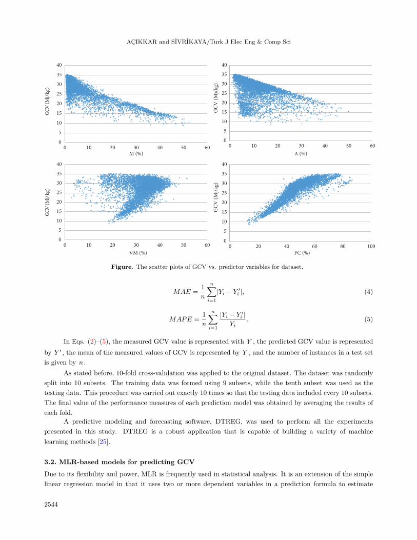
For this dataset, M, A, VM, and FC were selected as predictor variables and GCV was selected as thetarget variable. Although the predictor variables M, A, and VM were obtained by measuring in laboratoryenvironment, the predictor variable FC was calculated using M, A, and VM. The calculation of FC is given inEq. (1).

FC = 100− (M +A+ VM). (1)

Table 1 presents the descriptive statistics of the dataset. The scatter plots of GCV vs. predictor variablesare shown in Figure 2.

Table 1. Descriptive statistics of the dataset.

Category Variable name Minimumvalue

Maximumvalue Range Mean Standard

deviation

Predictor variables

M (%) 0.40 52.50 52.10 8.13 9.97A (%) 0.90 54.70 53.80 11.80 7.30VM (%) 3.00 51.96 48.96 32.02 6.51FC (%) 12.70 87.00 74.30 48.06 11.26

Target variable GCV (Mj/kg) 8.82 36.26 27.44 26.91 5.35

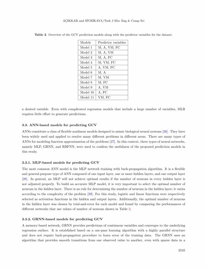
3. Methodology and prediction models3.1. MethodologyFor the analyzed dataset, by using combinations of the predictor variables M, A, VM, and FC, 11 models werecreated to determine the effectiveness of each predictor variable for predicting GCV of coal. Table 2 shows theprediction models for GCV and the predictor variables that each model has.

In this study, MLR-, MLP-, GRNN-, and RBFNN-based prediction models were utilized for predictingGCV of coal. The results of the presented GCV prediction models were compared with each other.

10-fold cross-validation was used for satisfying the generalization of GCV prediction models. Theprediction performance of the presented GCV models were computed by using the following metrics: R2 ,RMSE , MAE , and MAPE . The formulas of these performance metrics are shown in Eqs. (2)–(5).

R2 = 1−

n∑i=1

(Yi − Y ′i )

2

n∑i=1

(Yi − Y )2, (2)

RMSE =

√√√√ 1

n

n∑i=1

(Yi − Y ′i )

2, (3)

2543


0

5

10

15

20

25

30

35

40

0 10 20 30 40 50 60

)gk/jM(

VC

G

M (%)

0

5

10

15

20

25

30

35

40

0 10 20 30 40 50 60

GC

V (

Mj/

kg)

A (%)

0

5

10

15

20

25

30

35

40

0 10 20 30 40 50 60

)gk/jM(

VC

G

VM (%)

0

5

10

15

20

25

30

35

40

0 20 40 60 80 100

GC

V (

Mj/

kg)

FC (%)

Figure. The scatter plots of GCV vs. predictor variables for dataset.

MAE =1

n

n∑i=1

|Yi − Y ′i |, (4)

MAPE =1

n

n∑i=1

|Yi − Y ′i |

Yi. (5)

In Eqs. (2)–(5), the measured GCV value is represented with Y , the predicted GCV value is representedby Y ′ , the mean of the measured values of GCV is represented by Y , and the number of instances in a test setis given by n .

As stated before, 10-fold cross-validation was applied to the original dataset. The dataset was randomlysplit into 10 subsets. The training data was formed using 9 subsets, while the tenth subset was used as thetesting data. This procedure was carried out exactly 10 times so that the testing data included every 10 subsets.The final value of the performance measures of each prediction model was obtained by averaging the results ofeach fold.

A predictive modeling and forecasting software, DTREG, was used to perform all the experimentspresented in this study. DTREG is a robust application that is capable of building a variety of machinelearning methods [25].

3.2. MLR-based models for predicting GCVDue to its flexibility and power, MLR is frequently used in statistical analysis. It is an extension of the simplelinear regression model in that it uses two or more dependent variables in a prediction formula to estimate

2544


Table 2. Overview of the GCV prediction models along with the predictor variables for the dataset.

Models Predictor variablesModel 1 M, A, VM, FCModel 2 M, A, VMModel 3 M, A, FCModel 4 M, VM, FCModel 5 A, VM, FCModel 6 M, AModel 7 M, VMModel 8 M, FCModel 9 A, VMModel 10 A, FCModel 11 VM, FC

a desired variable. Even with complicated regression models that include a large number of variables, MLRrequires little effort to generate predictions.

3.3. ANN-based models for predicting GCV

ANNs constitute a class of flexible nonlinear models designed to mimic biological neural systems [26]. They havebeen widely used and applied to resolve many different problems in different areas. There are many types ofANNs for modeling function approximation of the problems [27]. In this context, three types of neural networks,namely MLP, GRNN, and RBFNN, were used to confirm the usefulness of the proposed prediction models inthis study.

3.3.1. MLP-based models for predicting GCV

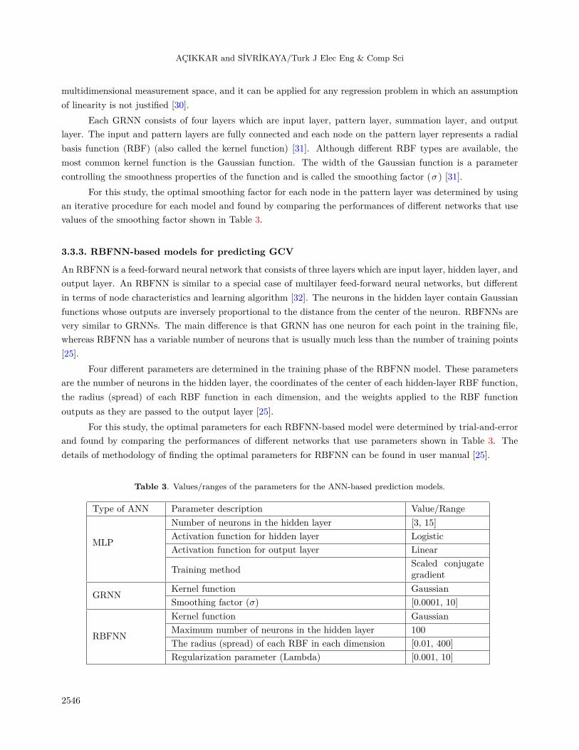
The most common ANN model is the MLP network training with back-propagation algorithm. It is a flexibleand general-purpose type of ANN composed of one input layer, one or more hidden layers, and one output layer[28]. In general, an MLP will not achieve optimal results if the number of neurons in every hidden layer isnot adjusted properly. To build an accurate MLP model, it is very important to select the optimal number ofneurons in the hidden layer. There is no rule for determining the number of neurons in the hidden layer; it variesaccording to the complexity of the problem [29]. For this study, logistic and linear functions were respectivelyselected as activation functions in the hidden and output layers. Additionally, the optimal number of neuronsin the hidden layer was chosen by trial-and-error for each model and found by comparing the performances ofdifferent networks that use values of number of neurons shown in Table 3.

3.3.2. GRNN-based models for predicting GCV

A memory-based network, GRNN provides predictions of continuous variables and converges to the underlyingregression surface. It is established based on a one-pass learning algorithm with a highly parallel structureand does not require back-propagation procedure to learn error of the training data. The GRNN uses analgorithm that provides smooth transitions from one observed value to another, even with sparse data in a

2545


multidimensional measurement space, and it can be applied for any regression problem in which an assumptionof linearity is not justified [30].

Each GRNN consists of four layers which are input layer, pattern layer, summation layer, and outputlayer. The input and pattern layers are fully connected and each node on the pattern layer represents a radialbasis function (RBF) (also called the kernel function) [31]. Although different RBF types are available, themost common kernel function is the Gaussian function. The width of the Gaussian function is a parametercontrolling the smoothness properties of the function and is called the smoothing factor (σ ) [31].

For this study, the optimal smoothing factor for each node in the pattern layer was determined by usingan iterative procedure for each model and found by comparing the performances of different networks that usevalues of the smoothing factor shown in Table 3.

3.3.3. RBFNN-based models for predicting GCV

An RBFNN is a feed-forward neural network that consists of three layers which are input layer, hidden layer, andoutput layer. An RBFNN is similar to a special case of multilayer feed-forward neural networks, but differentin terms of node characteristics and learning algorithm [32]. The neurons in the hidden layer contain Gaussianfunctions whose outputs are inversely proportional to the distance from the center of the neuron. RBFNNs arevery similar to GRNNs. The main difference is that GRNN has one neuron for each point in the training file,whereas RBFNN has a variable number of neurons that is usually much less than the number of training points[25].

Four different parameters are determined in the training phase of the RBFNN model. These parametersare the number of neurons in the hidden layer, the coordinates of the center of each hidden-layer RBF function,the radius (spread) of each RBF function in each dimension, and the weights applied to the RBF functionoutputs as they are passed to the output layer [25].

For this study, the optimal parameters for each RBFNN-based model were determined by trial-and-errorand found by comparing the performances of different networks that use parameters shown in Table 3. Thedetails of methodology of finding the optimal parameters for RBFNN can be found in user manual [25].

Table 3. Values/ranges of the parameters for the ANN-based prediction models.

Type of ANN Parameter description Value/Range

MLP

Number of neurons in the hidden layer [3, 15]Activation function for hidden layer LogisticActivation function for output layer Linear

Training method Scaled conjugategradient

GRNN Kernel function GaussianSmoothing factor (σ) [0.0001, 10]

RBFNN

Kernel function GaussianMaximum number of neurons in the hidden layer 100The radius (spread) of each RBF in each dimension [0.01, 400]Regularization parameter (Lambda) [0.001, 10]

2546


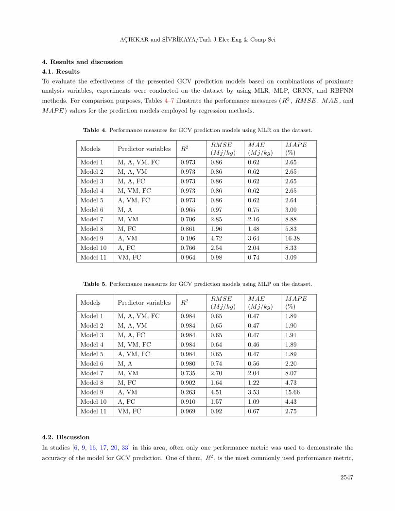
4. Results and discussion4.1. ResultsTo evaluate the effectiveness of the presented GCV prediction models based on combinations of proximateanalysis variables, experiments were conducted on the dataset by using MLR, MLP, GRNN, and RBFNNmethods. For comparison purposes, Tables 4–7 illustrate the performance measures (R2 , RMSE , MAE , andMAPE ) values for the prediction models employed by regression methods.

Table 4. Performance measures for GCV prediction models using MLR on the dataset.

Models Predictor variables R2 RMSE(Mj/kg)

MAE(Mj/kg)

MAPE(%)

Model 1 M, A, VM, FC 0.973 0.86 0.62 2.65Model 2 M, A, VM 0.973 0.86 0.62 2.65Model 3 M, A, FC 0.973 0.86 0.62 2.65Model 4 M, VM, FC 0.973 0.86 0.62 2.65Model 5 A, VM, FC 0.973 0.86 0.62 2.64Model 6 M, A 0.965 0.97 0.75 3.09Model 7 M, VM 0.706 2.85 2.16 8.88Model 8 M, FC 0.861 1.96 1.48 5.83Model 9 A, VM 0.196 4.72 3.64 16.38Model 10 A, FC 0.766 2.54 2.04 8.33Model 11 VM, FC 0.964 0.98 0.74 3.09

Table 5. Performance measures for GCV prediction models using MLP on the dataset.


MAE(Mj/kg)

MAPE(%)


4.2. DiscussionIn studies [6, 9, 16, 17, 20, 33] in this area, often only one performance metric was used to demonstrate theaccuracy of the model for GCV prediction. One of them, R2 , is the most commonly used performance metric,

2547


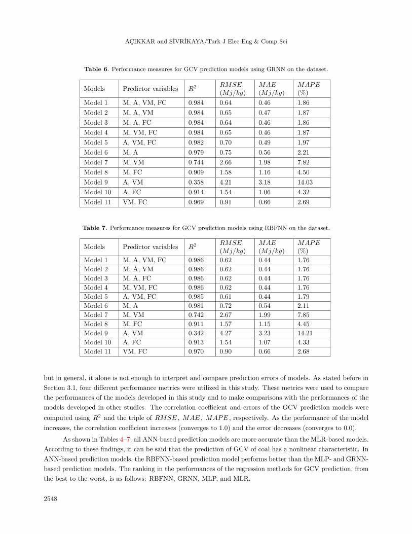
Table 6. Performance measures for GCV prediction models using GRNN on the dataset.


MAE(Mj/kg)

MAPE(%)


Table 7. Performance measures for GCV prediction models using RBFNN on the dataset.


MAE(Mj/kg)

MAPE(%)


but in general, it alone is not enough to interpret and compare prediction errors of models. As stated before inSection 3.1, four different performance metrics were utilized in this study. These metrics were used to comparethe performances of the models developed in this study and to make comparisons with the performances of themodels developed in other studies. The correlation coefficient and errors of the GCV prediction models werecomputed using R2 and the triple of RMSE , MAE , MAPE , respectively. As the performance of the modelincreases, the correlation coefficient increases (converges to 1.0) and the error decreases (converges to 0.0).

As shown in Tables 4–7, all ANN-based prediction models are more accurate than the MLR-based models.According to these findings, it can be said that the prediction of GCV of coal has a nonlinear characteristic. InANN-based prediction models, the RBFNN-based prediction model performs better than the MLP- and GRNN-based prediction models. The ranking in the performances of the regression methods for GCV prediction, fromthe best to the worst, is as follows: RBFNN, GRNN, MLP, and MLR.

2548


The errors of the models including quadruple and triple combinations of the predictor variables (Model1 to Model 5) are almost similar and these models have higher correlations and lower errors than the onesincluding dual combinations of predictor variables.

In general, it is desirable that the values of all the predictor variables used for a prediction model arecollected by measuring. However, sometimes it is seen that the value of a predictor variable is obtained bycalculation. If the calculation of a predictor variable value depends only on the other predictor variables, theinclusion of that variable to the model does not cause a noticeable increase in the accuracy of the predictionmodel. According to this approach, when comparing the performances of Model 1 and Model 2 for all regressionmethods, it is clear that the FC variable has a negligible effect on prediction. In addition, since the FC isderived from the other predictor variables (M, A, and VM), it gives higher correlations and lower errors in theother models including the FC variable.

The results show that addition of the predictor variables M and A into the prediction models has astrong positive effect and distinctively reduces error for GCV prediction. The ranking in the performance ofthe predictor variables except FC for GCV prediction, from the highest to the lowest, is as follows: M, A, andVM.

4.3. Comparing the results

It is to be noted that for most of the studies suggested in the literature, it is not possible to compare theirprediction results directly and in detail with those obtained in this study because each study a) uses differentdatasets which contain different numbers of samples, b) uses different datasets which have different datacharacteristics (e.g., coal rank and region extracted), c) uses different datasets which have different predictorvariables based on the analysis type, d) uses different types of prediction methods, and e) uses different datavalidation methods.

However, there are a few studies in the literature [6, 16, 20] that utilized the database COALQUALVersion 2.0 with 4540 entries which was a subset of the dataset used in this study (COALQUAL Version 3.0with 6520 entries). In addition, these studies used the same predictor variables based on proximate analysis,whereas they utilized different prediction and validation methods. Hence, a comparison can be made betweenthe performances of prediction models in this study and those of the mentioned studies [6, 16, 20].

Mesroghli et al. [16] developed a prediction model that includes the predictor variables M, A, and VM.Multivariable regression (corresponds to MLR) and feed-forward ANN (corresponds to MLP) methods wereapplied to this model. In contrast to the present study, they showed that the MLR-based model performsbetter than the MLP-based model for predicting GCV. For the MLR- and MLP-based models, the presentedR2 values were respectively 0.97 and 0.95 in their study, whereas the presented R2 values were respectively0.973 and 0.984 in the present study. According to these results, performances of the MLR-based models weresimilar to each other; however, prediction results of the MLP-based model developed in the present study aremore accurate than those of their study.

Tan et al. [6] proposed a prediction model based on support vector regression (SVR). According to theirstudy, for the SVR-based prediction model that includes the predictor variables M, A, VM, and FC, the averageabsolute error percentage (corresponds to MAPE ) was 2.42%. In the present study, for Model 1 given in Table7, MAPE value was 1.76%. In another study [20], Matin and Chelgani developed prediction models by usingthe multivariable regression (corresponds to MLR) and random forest (RF) methods. They also used M, A,

2549


and VM as predictor variables. The reported values of R2 for the MLR- and RF-based models were the same(0.97). According to the present study, for the RBFNN-based prediction model (Model 2 given in Table 7), theR2 value was obtained as 0.986. Hence, the results showed that the RBFNN-based prediction model proposedin the present study performs better than the SVR-based prediction model proposed in [6] and the RF-basedprediction model proposed in [20].

5. ConclusionThe objective of this work was to develop new models using MLR, MLP, GRNN, and RBFNN for predictionand show the discriminative predictor variables of GCV. The dataset was generated by using proximate analysesresults and GCV, belonging to 6520 coal samples in as-received basis. By using the combinations of the predictorvariables (M, A, VM, and FC), 11 models were developed for predicting GCV. For comparison purposes, theaforementioned regression methods were implemented to the models. 10-fold cross-validation was utilized forsatisfying the generalization capability of the developed models. The performances of the prediction modelswere stated by calculating the values of metrics R2 , RMSE , MAE , and MAPE .

Among the regression models, prediction models based on RBFNN exhibited better performances thanthe models developed by using MLR, MLP, or GRNN, irrespective of which variant of the predictor variablewas used. The MLR-based prediction models exhibited the worst performances for predicting GCV. On theother hand, MLR produced faster results compared to the other regression methods for prediction.

For all the results regarding regression methods, the same comments can be made for the effect of therelevant predictor variables, regardless of the regression method used. So the results reveal that, among thepredictor variables, M and A have more positive effect on the performance of GCV prediction. Besides, asdiscussed before, the variable FC has negligible or strong effect (since FC has information about other predictorvariables) in different models. The ranking in the performance of the predictor variables except FC for GCVprediction, in descending order, is M, A, and VM.

Taking into account the performances of all the models proposed in this study, the RBFNN-basedpredictor model that includes the predictor variables M, A, and VM can be the most suitable model for predictingGCV of coal.

References

[1] Sivrikaya O. Cleaning study of a low-rank lignite with DMS, Reichert spiral and flotation. Fuel 2014; 119: 252-258.

[2] Akkaya AV. Proximate analysis based multiple regression models for higher heating value estimation of low rankcoals. Fuel Process Technol 2009; 90: 165-170.

[3] de Souza KF, Sampaio CH, Kussler JAT. Washability curves for the lower coal seams in Candiota Mine - Brazil.Fuel Process Technol 2012; 96: 140-149.

[4] Yılmaz I, Erik NY, Kaynar O. Different types of learning algorithms of artificial neural network (ANN) models forprediction of gross calorific value (GCV) of coals. Sci Res Essays 2010; 5: 2242-2249.

[5] Chen W, Xu R. Clean coal technology development in China. Energy Policy 2010; 38: 2123-2130.

[6] Tan P, Zhang C, Xia J, Fang QY, Chen G. Estimation of higher heating value of coal based on proximate analysisusing support vector regression. Fuel Process Technol 2015; 138: 298-304.

[7] Patel SU, Jeevan Kumar B, Badhe YP, Sharma, BK, Saha S, Biswas S, Chaudhury A, Tambe SS, Kulkarni B.Estimation of gross calorific value of coals using artificial neural networks. Fuel 2007; 86: 334-344.

2550


[8] Llorente MJF, Garcia JEC. Suitability of thermo-chemical corrections for determining gross calorific value inbiomass. Thermochim Acta 2008; 468: 101-107.

[9] Majumder A, Jain R, Banerjee P, Barnwal J. Development of a new proximate analysis based correlation to predictcalorific value of coal. Fuel 2008; 87: 3077-3081.

[10] Spooner C. Swelling power of coal. Fuel 1951; 30: 193-202.

[11] Mazumdar BK. Coal systematics: deductions from proximate analysis of coal part I. J Sci Ind Res B 1954; 13:857-863.

[12] Given PH, Weldon D, Zoeller JH. Calculation of calorific values of coals from ultimate analyses: theoretical basisand geochemical implications. Fuel 1986; 65: 849-854.

[13] Mazumdar BK. Theoretical oxygen requirement for coal combustion: relationship with its calorific value. Fuel 2000;79: 1413-1419.

[14] Channiwala SA, Parikh PP. A unified correlation for estimating HHV of solid, liquid and gaseous fuels. Fuel 2002;81: 1051-1063.

[15] Parikh J, Channiwala S, Ghosal G. A correlation for calculating HHV from proximate analysis of solid fuels. Fuel2005; 84: 487-494.

[16] Mesroghli S, Jorjani E, Chehreh Chelgani S. Estimation of gross calorific value based on coal analysis using regressionand artificial neural networks. Int J Coal Geol 2009; 79: 49-54.

[17] Chelgani SC, Mesroghli S, Hower JC. Simultaneous prediction of coal rank parameters based on ultimate analysisusing regression and artificial neural network. Int J Coal Geol 2010; 83: 31-34.

[18] Erik NY, Yilmaz I. On the use of conventional and soft computing models for prediction of gross calorific value(GCV) of coal. Int J Coal Prep Util 2011; 31: 32-59.

[19] Feng Q, Zhang J, Zhang X, Wen S. Proximate analysis based prediction of gross calorific value of coals: a comparisonof support vector machine, alternating conditional expectation and artificial neural network. Fuel Process Technol2015; 129: 120-129.

[20] Matin SS, Chelgani SC. Estimation of coal gross calorific value based on various analyses by random forest method.Fuel 2016; 177: 274-278.

[21] Akhtar J, Sheikh N, Munir S. Linear regression-based correlations for estimation of high heating values of Pakistanilignite coals. Energy Sources Part Recovery Util Environ Eff 2017; 39: 1063-1070.

[22] Wen X, Jian S, Wang J. Prediction models of calorific value of coal based on wavelet neural networks. Fuel 2017;199: 512-522.

[23] Ozbayoglu AM, Ozbayoglu ME, Ozbayoglu G. Regression techniques and neural network for the estimation of grosscalorific value of turkish coals. In: XIIth International Mineral Processing Symposium; 6-8 October 2010; Nevsehir,Turkey. pp. 1175-1180.

[24] Ozbayoglu AM, Ozbayoglu ME, Ozbayoglu G. Comparison of gross calorific value estimation of turkish coals usingregression and neural networks techniques. In: XXVIth International Mineral Processing Congress (IMPC 2012);24-28 September 2012; New Delhi, India. pp. 4011-4023.

[25] Sherrod PH. DTREG predictive modeling software user manual. 2014.

[26] Rooki R. Application of general regression neural network (GRNN) for indirect measuring pressure loss of Herschel-Bulkley drilling fluids in oil drilling. Measurement 2016; 85: 184-191.

[27] Park JW, Venayagamoorthy GK, Harley RG. MLP/RBF neural-networks-based online global model identificationof synchronous generator. IEEE Trans Ind Electron 2005; 52: 1685-1695.

[28] Mashaly AF, Alazba AA. MLP and MLR models for instantaneous thermal efficiency prediction of solar still underhyper-arid environment. Comput Electron Agric 2016; 122: 146-155.

2551


[29] Abut F, Akay MF, George J. Developing new VO2max prediction models from maximal, submaximal and ques-tionnaire variables using support vector machines combined with feature selection. Comput Biol Med 2016; 79:182-192.

[30] Specht DF. A general regression neural network. IEEE Trans Neural Netw 1991; 2: 568-576.

[31] Ren S, Gao L. Combining artificial neural networks with data fusion to analyze overlapping spectra of nitroanilineisomers. Chemom Intell Lab Syst 2011; 107: 276-282.

[32] Arliansyah J, Hartono Y. Trip attraction model using radial basis function neural networks. Procedia Eng 2015;125: 445-451.

[33] Chehreh Chelgani S, Makaremi S. Explaining the relationship between common coal analyses and Afghan coalparameters using statistical modeling methods. Fuel Process Technol 2013; 110: 79-85.

2552

Date post:	20-Jan-2023
Category:	Documents
Upload:	khangminh22
View:	0 times
Download:	0 times

Prediction of gross calorific value of coal based on proximate ...

Documents