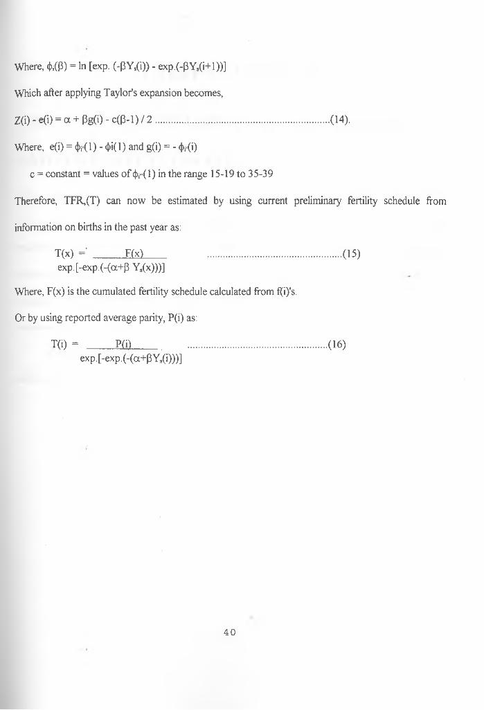
THE PROXIMATE DETERMINANTS OF FERTILITY: EVIDENCE FROM THE 1993 KENYA

DEMOGRAPHIC AND HEALTH SURVEY'*

'

THIS THESIS IS SUBMITTED IN PARTIAL FULFILMENT FOR

THE DEGREE OF MASTER OF SCIENCE IN POPULATION STUDIES

AT THE UNIVERSITY OF NAIROBI

MARCH 1998

UNIVERSITY OF NAIROBI LIBRARY

DECLARATION

This thesis is my original work and has not been represented for a degree in any other university.

Signature

Mutetei kavali

This thesis has been submitted for examination with my approval as university supervisor

Signature _Dr. Kimani

/

DEDICATION

To my dear spouse Muem and my two children Vincent and Fiona, who paid the price of staying many

days without me during my studies.

in

ACKNOWLEDGEMENTS

My very sincere appreciation goes to my supervisor Dr. Kimani without whose positive

criticism, motivation and guidance this thesis could not have been completed. I must also mention the

part played by Mr. Agwanda as my second supervisor before he left the country for further studies as

equally important towards the completion of this work.

I also gratefully acknowledge the generosity extended to me by the United Nations Fund for

Population Activities (UNFPA) for awarding me a full scholarship. This enabled me to pursue my

master of science degree course in population studies at the University of Nairobi without a lot of

financial problems. The co-operation and assistance given to me by the staff and students at the_

Population Studies and Research institute cannot go unmentioned.

To my parents, family members, and friends, I do extend my most sincere gratitude for your

invaluable encouragement both morally and financially during the course of my studies.

Finally, I am grateful to Jeremiah Muteti and the entire staff of LANsre CONSULTANTS from

where I was greatly assisted in typing and printing of this thesis.

IV

ABSTRACT

The main objective of this study was to determine the fertility levels and differentials of various

sub-groups in Kenya and to explain these differentials using the intermediate fertility variables. The sub­

groups considered in the study were the regions, place of residence, and levels of education. The

intermediate fertility variables that were studied were postpartum infecundability, non-marriage and

contraception.

The study used the Bongaarts’ model to estimate the indices for each intermediate fertility

variable and also to estimate the resulting total fertility rates for each sub-group. These fertility rates

were compared with those obtained from the Gomperrtz relational model which was chosen as.an

independent method of estimating fertility. The Bongaarts’-Kirmeyer regression equation of predicting

fertility rate given the contraceptive prevalence rate was also used to predict fertility by the regions.

The data used in this study was the Kenya demographic and health survey conducted in 1993.

The study found out that there was a general trend of decline in fertility among the regions,

place of residence and by the levels of education between the period 1989 and 1993. The study also

showed that at the national level as well as among five of the seven regions, the index of postpartum

infecundability was the lowest followed by that of non-marriage, then contraception. This implies that

the most important fertility inhibiting variable was lactation, followed by non-marriage, then

contraception. This agreed closely with Wamalwas’ findings of 1991 using the 1989 Kenya

demographic and health survey.

According to this study, lactation reduced total fecundity by 39.3 percent while non-marriage

and contraception reduced the total fecundity by 34 percent and 29.2 percent respectively. According

to Wamalwa, these percentages were 36, 26 and 18 respectively. Thus there has been a general

increase in the effect of these intermediate fertility variables in reducing fertility between these two

v

periods which, a fact that is supported by the general decline in fertility mentioned above. The study

also points out that contraception reduces fertility most among women in Nairobi, Central province

and those with secondary and higher level of education. Non-marriage had the greatest fertility

reducing effect among women in urban areas.

The other important finding of this study was that contraception was shown to have taken a

leading role in reducing fertility during the period 1989 to 1993. This is attributed to the highest

percent difference in the fertility reducing effect due to contraception of 11.2 percent compared to that

of 8.0 percent due to non-marriage and 3.3 percent due to breastfeeding or lactation. It was shown that

there was positive linear relationship between contraceptive prevalence rate and the level of fertility

among the sub-groups. This relationship was used to show how future demand for contraceptives

could be projected.

From these findings we were able to recommend that family planning programmes should be

intensified in those regions with high fertility like western, Nyanza and Rift valley. Universal education

especially for girls was also recommended since there existed direct relationship between the level of

education and the use of contraceptives.

vi

TABLE OF CONTENTSTOPIC PAGE

Title--------------------------------------------------------------------------------------------------------------------- i

Declaration------------------------------------------------------------------------------------------------------------ ii

Dedication------------------------------------------------------------------------------------------------------------- iii

Acknowledgements-------------------------------------------------------------------------------------------------iv

Abstract---------------------------------------------------------------------------------------------------------------- v

Table o f Contents---------------------------------------------------------------------------------------------------- vii

List o f Figures------------------------------------------------------------------------------------------------------- ix

List of Tables---------------------------------------------------------------------------------------------------------x

CHAPTER ONE:

INTRODUCTION-------------------------------------------------------------------------------------------------- 1

1.1 Background------------------------------------------------------------------------------------------------1

1.2 Statement o f the problem-------------------------------------------------------------------------------7

1.3 General Objective-----------------------------------------------------------------------------------------8

1.3.1 Specific Objectives------------------------------------------------------------------------------------ 8

1.4 Justification o f the Study--------------------------------------------------------------------------------9

1.5 Scope and Limitations o f th e -------------------------------------------------------------------------- 9

CHAPTER TWO:

LITERATURE REVIEW AND THEORETICAL FRAMEWORK

2.1 Literature Review---------------------------------------------------------------------------------------- 11

2.2 Application o f the various Models--------------------------------------------------------------------15

2.3 Conceptual Framework---------------------------------------------------------------------------------24

2.4 Operational Framework---------------------------------------------------------------------------------25

2.5 Operational Hypotheses---------------------------------------------------------------------------------26

CHAPTER THREE:

METHODS OF DATA COLLECTION AND ANALYSIS--------------------------------------------- 27

3.1 Sources o f D ata------------------------------------------------------------------------------------------- 27

3.2 Methods o f Data Analysis----------------------------------------------------------------------------- 28

3.3 Bongaarts’ M odel----------------------------------------------------------------------------------------28

3.4 Bongaarts’-Kirmeyer Model-------------------------- -»t----------------------------------------------35

3.5 Gompertz Relational M odel--------------------------------------------------------------------------- 36

3.5.1 Theoretical Background o f the M odel---------------------------------------------------------- 37

vii

CHAPTER FOUR:

the proxim ate d eter m in a n ts of fer tilitya n d fertility estim a tes

4.1 Introduction----------------------------------------------------------------------------------------------- 41

4.2 Background characteristics of female respondents----------------------------------------------- 42

4.3 Estimation of Indices by the Sub-groups------------------------------------------------------------43

4.3.1 Estimation o f the index of infecundability, Ci__________________________________ 44

4.3.2 Estimation of the index of Non-marriage, Cm__________________________________ 48

4.3.3 Estimation of the index of Contraception, Cc__________________________________ 50

4.4 Estimation o f the Model TFR from the indices----------------------------------------------------53

4.5 Estimation o f TFR using the Gompertz Relational M odel------------------------------------- 55

4.6 Comparison of the two Model TFR’S--------------------------------------------------------------- 61

4.7 Estimation of the role of each proximate determinant in reducing fertility-----------------62

4.8 The impact of the proximate determinants on fertility using the percent

reduction in fertility............................................... 67

4.9 Estimating the Predicted TFR using the Bongaarts’-Kirmeyer M odel................... 75

4.10 Projecting Fertility and future demand for Contraceptives---------------------------------- 77

CHAPTER FIVE:

SUMMARY, CONLUSIONS AND RECOMMENDATIONS--------------------------------------- 80

5.1 Introduction----------------------------------------------------------------------------------------------- 80

5.2 Summary of the findings--------------------------------------------------------------------------------81

5.3 Conclusions----------------------------------------------------------------------------------------------- 85

5.4 Policy Recommendations-------------------------------------------------------------------------------87

5.5 Recommendations for further Research...............................................................................-88

BIBLIOGRAPHY-------------------------------------------------------------------------------------------------- 89

APPENDIX A ------------------------------------------------------------------------------------------------------ 92

APPENDIX B ------------------------------------------------------------------------------------------------------ 114

>

vm

LIST OF FIGURESFIGURE--------------------------------------------------------------------------------------- PAGE

1. The Bongaarts’ Framework----------------------------------------------------------------------------------- 31

2. Operational Framework-----------------------------------------------------------------------------------------32

IX

LIST OF TABLESTABLE--------------------------------------------------------------------------------------------------------- PAGE

1.1 Total fertility rates among women aged 15-49 by the provinces, according to

Survey and percentage decrease by the provinces o f Kenya 1977-1993------------------------- 4

1.2 Observed TFR by education and place o f residence according to survey and the

Percentage decrease------------------------------------------------------------------------------------------- 5

1.3 Proximate determinants by the sub-groups, 1977-1978 and the observed TFR---------------- 6

1.4 Proximate determinants by, 1989 and observed TFR -------------------------------------------------6

4.1 Percent distribution of women, births in the last year (BL12), proportion married and

contracepting by regions------------------------------- 42

4.2 Percent distribution o f women, births in the last year (BL12), proportion married

and contracepting by levels of education.-----------------------------------------------------------------43

4.3 Percent distribution o f women, births in the last year (BL12), proportion married

and contracepting by place of residence------------------------------------------------------------------- 43

4.4 Births occurring 0-35 months, exactly 36 months before the survey and number

currently breastfeeding by age group of the m others.................................................................46

4.5 The prevalence (P), Incidence (I) and mean duration o f breastfeeding (B) by all

the sub-groups--------------------------------------------------------------------------------------------------47

4.6 Mean duration o f breastfeeding and the index of lactation, Cj_________________________ 48

4.7 Female population, number married, proportion married, BL12, age specific

fertility rates and age specific marital fertility ra te s --------------------------------------------------- 50

4.8 Estimation o f the index of contraception----------------------------------------------------------------- 51

4.9 Summary of the three proximate determinants of fertility-------------------------------------------- 52

4.10 The indices o f non-marriage, contraception, lactation and the model T F R ------------------- 54

4.11 Computed values o f F(i), F(x), and F(x) / F (x+ 5)----- ----------------------------------------------58

4.12 Computed values o f Z(x), Z(x) - e (x )------------------------------------------------------------------- 58

4.13 Computed values o f YA(x), FA(x), and TFR--------- ------------------------------------------------- 59

4.14 Total fertility rates obtained using Bongaarts’ model and those from the

Gompertz relational model----------------------------------------------------------------------------------------60

4.15 The indices o f non-marriage, lactation and contraception at the national level---------------63

4.16 The indices of non-marriage, lactation and contraception by the regions------------------ 64

417 The indices’of non-marriage, lactation and contraception by levels o f education------------ 66

4 18 The indices o f non-marriage, lactation and contraception by place of residence--------------66

x

4.19 The values o f C, TN, C-TN and percent reduction in fertility due to lactation

by the regions------------------------------------------------------------------------------------------------- 68

4.20 The values o f C, TN, C-TN and percent reduction in fertility due to lactation

by the levels o f education---------------------------------------------------------------------------------- 69

4.21 The values of C, TN, C-TN and percent reduction in fertility due to lactation

by place o f residence---------------------------------------------------------------------------------------- 70

4.22 The values o f TN, TM-TN, and the percent reduction in fertility due to

contraception by the regions-------------------------------------------------------------------------------70

4.23 The values o f TN, TM-TN, and the percent reduction in fertility due to

contraception by levels of education and place of residence---------------------------------------71

4.24 The values o f TM, TFR, TM-TFR and the percent reduction in fertility due to

non-marriage by the regions--------------------------------------------------------------------------------72

4.25 The values of TM, TFR, TM-TFR and the percent reduction in fertility due to

non-marriage by levels of education and place of residence-------------------------------------- 73

4.26 The percent reduction in fertility due to lactation, non-marriage and contraception

among women by regions between the period 1989 to 1993-------------------------------------- 74

4.27 The observed TFR, contraceptive prevalence rate and the predicted TFR by

regions..............................................................................................................................................76

4.28 Projected TFR and the rates o f fertility decline for given periods at the national

level--------------------------------------------------------------------------------------------------------------- 78

xi

CHAPTER ONE

INTRODUCTION

1.1 BACKGROUND

Most studies of the causes of fertility trends and differentials have sought to measure the

impact of socio-economic factors on fertility. These factors include income, education, and place of

residence among others that have been readily available and easily manipulated to influence fertility.

Unfortunately, the results o f these studies have been far from being conclusive. Not infrequently,

relationships have been found to differ not only in magnitude but even in direction in different settings

and at different times ( Rodriguez and Cleland 1987). Therefore to improve understanding of the

causes of fertility variation, it has been necessary to analyse the mechanisms through which these socio­

economic variables influence fertility. In response to this need, studies are being undertaken on the

proximate determinants of fertility.

The proximate determinants of fertility are the biological and behavioural factors through

which social, economic and environmental variables affect fertility; the principal characteristic of a

proximate determinant being its direct influence on fertility. To explain fertility differentials among

populations as well as the trends in fertility over time, we need to look at variations in one or more of

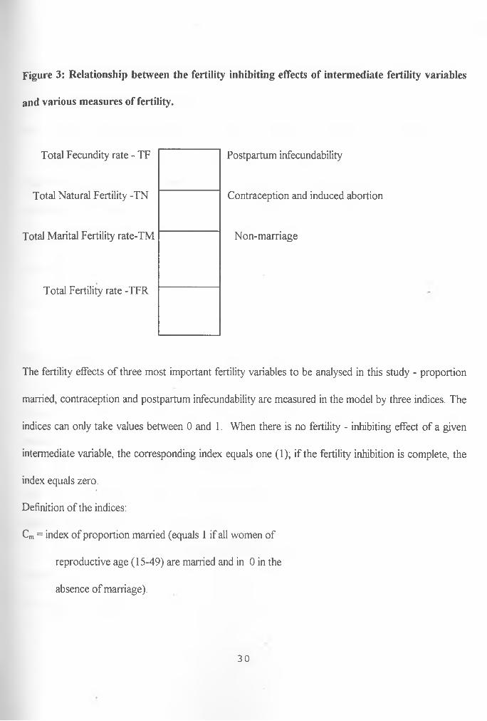
the proximate determinants. Bongaarts et al (1984) enumerated nine proximate determinants of

fertility. Among them, the four most important ones are; Marriage patterns, Postpartum

infecundability, Contraceptive use, and Induced abortion.

1

These four determinants of fertility represent factors that directly affect fertility and do vary

across different cultures. The percentage of women married determines the number of women exposed

to the risk of becoming pregnant. The greater the number of women exposed the higher the resulting

fertility. On the other hand, contraception delays or limits the number of children being bom which

clearly affects a society's fertility level.

The practice of breastfeeding and sexual abstinence after the birth of a child reduces a woman's

exposure to becoming pregnant. Breastfeeding of long duration and on demand delays the return of a

woman's normal pattern of ovulation. This in return affects the fertility of a woman. Induced abortion

includes any practice that deliberately interrupts the normal course of gestation and therefore affects a

society's level of fertility.

Other proximate determinants such as the level of natural sterility and the rate of spontaneous

abortion tend to be fairly constant across populations, and hence do not contribute much toward

explaining fertility differences between populations or over time within the same population.

During the periods 1984-1988 and 1989-1993, fertility dropped by about 20 percent, this being

the most dramatic decline in fertility ever recorded in Kenya and one of the most dramatic recorded

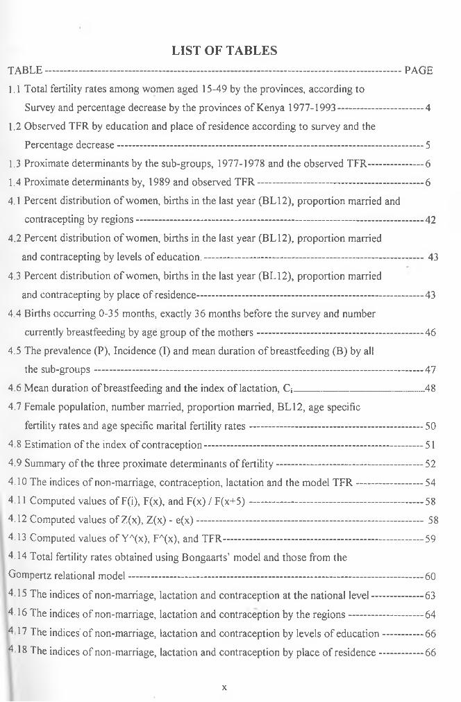
elsewhere. Table 1 gives the total fertility rates among women aged 15-49 by the provinces. Fertility

decline varied considerably among provinces. A comparison of the 1977-1978 KFS data with the 1993

KDHS data in table 1 shows declines in all provinces. Major fertility declines were recorded in

Nairobi, Rift Valley and Central Provinces. For example fertility in Central Province fell from an

average of 8.6 to 3.9 children per woman over 15 years. KDHS results show that as fertility decline,

the differentials among provinces increased. In 1977-1978, women in Rift Valley Province had an

2

*

average of 2.7 more live births than their counterparts in Nairobi (8.8 and 6.1); this difference between

provinces with the highest and the lowest fertility had increased to 3.5 births by 1989 and to 3.0 births

by 1993 (8.1 and 6.4 in Western Province Vs 4.6 and 3.4 in Nairobi).

Fertility differentials by education and place of residence have also been studied. Table 2 below

gives the observed total fertility rate by education and place of residence, according to survey and the

percentage decline in fertility in the period 1977-1993. From the table, it can be seen that there has

been a dramatic decline in fertility of more than 30 percent in the period 1977-1993 except for the

women with no education whose percentage decline is 26.0. The highest decline in fertility has been

recorded among women living in the urban areas, a decline of 43 percent within the period 1977-3993.

Comparing data from the 1977-1978 Kenya fertility Survey (KFS), the 1984, 1989 and 1993

Kenya demographic and health survey (KDHS) by the regions, it can be seen that the TFR declined

from a high 8.1 children per woman in 1977-1978 to 7.7 in 1984, 6.7 in 1989 and further down to 5.4

in 1993. This gives a total decrease of 33 percent.

3

V

Table 1.1 Total fertility rates among women aged 15-49, by Province, according to survey: andpercentage decrease by Province, Kenya, 1977-1993.

PROVINCE 1977-1978KFS

1984KCPS

1989I w i l J

1993 %a c i r

1977-93

Total 8.1 7.7 6.7 5.4 33.3

Western 8.2 6.3 8.1 6.4 21.9

Nyanza 8.0 8.2 7.1 5.8 27.5

Rift Valley 8.8 8.6 7.0 5.7 35.2

Central 8.6 7.8 6.0 3.9 54.7

Nairobi 6.1 5.6 4.6 3.4 44.3

Eastern 8.2 8.0 7.0 5.9 "28.0

Coast 7.2 6.7 5.5 5.3 26.4

Source: (1) Central Bureau of Statistics (CBS), First Report, KCPS 1984, Nairobi, 1984.(2) NCPD and Institute for Research Development, DHS, 1989 and 1993, Nairobi

Kenya.(3) CBS, First Report, KFS 1977-1978, Nairobi, Kenya, 1980.

4

V

Table 1.2 Observed total fertility rate by Education and place of residence, according tosurvey and percentage decrease.

Subgroup 1977-1978 KFS 1989 KDHS 1993 KDHS % DECLINE 1977-1993

Kenya 8.15 6.62 5.40 33.7

Urban 6.07 4.71 3.44 43.3

Rural 8.36 6.98 5.80 30.6

No Education 8.15 7.23 6.03 26.0

1-4 years 8.97 7.65 6.18 31.1

5-7 years 7.91 7.15 5.02 36.5

8+ years 6.95 4.95 4.03 42.0

Source:(l) Population dynamics of Kenya pg. 106-9

(2) Demographic and Health Survey, Kenya, 1993.

The above mentioned fertility differentials and trends as well as the decline over the period

1977-1993 may be well explained by looking at the variations which may have taken place on the

proximate determinants of fertility. Results from the 1977-1978 KFS data indicated that postpartum

infecundability was the most important fertility-inhibiting variable at the national level. Marriage

pattern followed in significance, with contraception having a relatively minor effect during this earlier

period. The national research council (NRC, 1993) analysed the proximate determinants of fertility

using the 1989 KDHS data. At the national level, they found out that the most important inhibiting

index was postpartum infecundability, followed by contraception and then the marriage pattern. Tables

1.3 and 1.4 below give the three most important proximate determinants by subgroups for the period

1977-1978 and 1989 respectively.

5

Table 1.3 Proximate Determinant by Subgroup, 1977-1978 and the observed total fertility rate.

Subgroup Observed TFR Index of Mairiage, CM

Index of Contraceptive

Cc

Index of Postpartum

infecutidabiiity, O

National 8.15 0.91 0.95 0.64

Urban 6.07 0.84 0.89 0.69

Rural 8.36 0.92 0.96 0.64

No Education 8.15 0.96 0.97 0.61

1-4 years 8.97 0.93 0.95 0.64

5-7 years 7.91 0.90 0.93 0.69

8+ years 6.95 0.83 0.83 0.70

Source: Population Dynamics of Kenya pg. 106-7

Table 1.4 Proximate Determinants by Subgroup, 1989 and the observed total fertility rate.

Subgroup Observed TFR Index of Marriage, Cm

Index ofContraception, Cc.

Index of Postpartum

Jnfecundability

National 6.62 0.86 0.76 0.66

Urban 4.71 0.82 0.71 0.70

Rural 6.98 0.81 0.77 0.66

No Education 6.98 0.87 0.71 0.70

1-4 years 7.65 0.94 0.77 0.65

5-7 years 7.15 0.88 0.74 0.69

8+ years 4.95 0.82 0.65 0.71

Source: (1) Population Dynamics of Kenya, pg. 108-9

Wamalwa (1991) also analysed the proximate determinants o f fertility using the 1989 KDHS

data. He found out that the most important fertility-inhibiting factor was postpartum infecundability.

However, his second most important fertility inhibiting factor was still marriage patterns (as was the

case in 1977-1978), while contraception played the least role in reducing fertility.

1.2 Statement of the Problem

From the studies undertaken using the 1989 KDHS DATA on the proximate determinants of

fertility, it is evident that there is a consistency as well as a contradiction between Wamalwa's findings

and those from the National Research Council. Wamalwa (1991) and the NRC (1993) found out that

the most important proximate determinant was postpartum infecundability. However, Wamalwa

(op.cit) found out that the second most important fertility inhibiting factor was marriage patterns, while

the NRC (1991) showed that this factor had been overtaken by contraception. Thus the second most

important factor inhibiting fertility was different although the data source was the same. With this

contradiction in place and the fact that the role played by each proximate determinant changes with

time, this study aims at determining the role played by each of the three intermediate fertility variables

using the most recent data, the 1993 Kenya Demographic and Health Survey. Contraceptive

prevalence has increased sharply in most developing countries in the recent past. For example in Kenya,

the prevalence rate has increased from 6% in 1977-1978 to 14% in 1984, then to 27% in 1989 and to

33% by 1993. The total fertility rate has also been going down from 8.1 in 1977-1978, 7.7 in 1984, 6.7

in 1989 and down to 5.4 in 1993. Due to this strong linear relationship between the prevalence rate

among married women and the TFR, contraception is widely being said to be the major cause of

fertility decline in many developing countries. In some cases, the observed TFR does not match the

7

f

predicted value from the prevalence rate. The basic question therefore is what is the situation by

regions in Kenya? Does the observed TFR match the prevalence rates? These two questions along

with the fore- mentioned contradiction are mainly the issues of concern, which need to be investigated

in this study.

1.3 General Objective

The general objective of this study is to determine and account for the fertility levels of various

sub-groups in Kenya by applying the Bongaarts' model on the 1993 KDHS data.

1.3.1 Specific Objectives

(i) To estimate fertility levels by regions, education and place of residence using

Bongaarts' model (model estimate of TFR).

(ii) To estimate fertility by regions, education and place of residence using the Gompertz

relational model and compare it with (i) above.

(iii) To determine the contribution of each of the three fertility inhibiting factors on

fertility by the subgroups.

(iv) To determine the predicted TFR using the Bongaarts'-Kirmeyer regression equation.

(v) To determine regions with excess fertility (those with higher observed TFR than the

predicted one).

(vi) To project fertility and hence demand for future contraceptives.

8

1.4 Justification of the Study

The study is aimed at undertaking an analysis of the proximate determinants of fertility and will

enable us to determine the most recent causes of fertility differences in Kenya. From this study, it may

be possible to estimate how much each or all of the proximate determinants may be modified to obtain

a given reduction in fertility. This may enable projections into future fertility declines, which is of great

interest and importance to the planners and policy makers.

The study is going to give an evaluation of the achievement o f family planning programme in

reducing fertility in various regions of the country. It will also help to project future demand for

contraception, which is a major policy idea.

The study is also expected to open up new areas of research for interested future researchers.

1.5 Scope and Limitations of the Study

This study uses data from the 1993 Kenya Demographic and Health Survey. The analysis has been

limited to the data collected from 7540 women aged 15-49 years. The survey covered all areas of

Kenya except all .the districts in North -Eastern province and four other northern districts - Samburu,

Turkana in Riff-valley and Isiolo and Marsabit in Eastern province - all of which contain less than 4%

of the country's population. The 1993 KDHS is limited to data on abortion. This is mainly because

abortion is not legalised and therefore obtaining data on it is very difficult. This study therefore does

not estimate the index of abortion. The data is also insufficient for any reasonable district analysis to be

done and hence the analysis is largely going to be done by the provinces.

9

Methodology limitations include the errors in measurement of the proximate determinants, and

those arising in the specification of the model. The figure of TF to be used in the analysis will only be

an approximation since TF is a function of the other three proximate determinants not explicitly

included in the model (i.e. natural fecundity, intra-uterine mortality and permanent sterility).

10

CHAPTER TWO:

LITERATURE REVIEW AND THEORETICAL

FRAMEWORK

2.1 LITERATURE REVIEW

Investigations into the proximate determinants of fertility go all the way back to the mid 1950s.

Davis (1956) constructed the first detailed mathematical models of the reproductive process.

Following this pioneering work, other researchers did further investigations during the 1960's most

notably Potter (1963), Sheps (1964) and Tietoze (1964).

Since Davis and Blake’s (1956) seminar paper on the proximate determinants of fertility, many

such frameworks have been proposed. Davis and Blake recognised the fact that fertility differences

among populations and trends in fertility over time can always be traced to variations in one or more of

the proximate determinants. Starting from the premise that reproduction involves three necessary steps

of intercourse, conception and completion of gestation, they identified a set of 11 proximate

determinants that they called "intermediate fertility variables".

Davis and Blake framework of 1956 with 11 intermediate variables has been divided into the

following three categories:-

I. Factors affecting exposure to intercourse

1. Age of entry into sexual unions

11

2. Permanent celibacy: proportion of women never

• entering sexual unions.

3. Amount of reproductive period spent after or between unions.

4. Voluntary abstinence.

5. Involuntary abstinence (from illness, impotence, unavoidable but

temporary separations).

6. Coital frequency (excluding periods of abstinence).

II. Factors affecting exposure to conception.

7. Fecundity or infecundity as affected by involuntary causes.

8. Use or non-use of contraception

a) By mechanical and chemical means.

b) By other means.

9. Fecundity or infecundity, as affected by voluntary causes (sterilisation, sub­

incision, medical treatment, etc.).

ID. Factors affecting gestation and successful parturition.

10. Foetal mortality from involuntary causes

11. Foetal mortality from voluntary causes.

Bongaarts (1978) then improved on the Davis and Blake model and came up with his model

which contains a set of eight intermediate variables: proportion married, contraception usage and

effectiveness, prevalence of induced abortion, duration of postpartum infecundability, frequency of

intercourse (fecundability), spontaneous intrauterine mortality, prevalence of permanent sterility and

12

duration of the fertile differences. He further showed that among these four, lactation plays the most

important role in tropical Africa. Bongaarts' model can be used to estimate how much one or a

combination of several of the intermediate fertility variables has to be modified to obtain a given

reduction in fertility.

Most of the other earlier efforts focused on the construction of increasingly more realistic but

sometimes highly complex models for the relationship between fertility and the proximate determinants

of fertility. This development has continued into the 1980s and relatively simple yet quite realistic

fertility models now exist. The construction of these models and their validation has been made

possible by the greatly increased availability of empirical measures of the proximate variables in many

populations. The. resulting improvement in the understanding of the fertility effect of the proximate

determinants has led to a more frequent inclusion of the proximate factors in studies of socio-economic

and environmental determinants of fertility (for example Bongaarts 1980, Laesthaeghe 1982, Shah and

Page 1982).

Gaslonde (1982) developed the sexual activity table (SAT) which can be included in

the survey to gain information on the exposure status of each woman for each month preceding the

survey over the period of interest, usually 12 months. Each woman can then be classified into one of

the following exposure state for each month covered by SAT: pregnant, absence of sexual relations,

sexual relations using effective contraception, sexual relations using inefficient contraception, sexual

relations using no contraception. From the data obtained from SAT, the reducing effect of the absence

> of sexual relations, Tasr, the reducing effect of contraceptive practice, rep, and the reducing effect of

foetal mortality, be estimated using simple relationships and a model set to associate the theoretical

13

fertility rate, P, (which is defined as the rate that would have been achieved had all the women had

sexual relations regularly without using any means of deliberate fertility control) and which is similar in

concept to Bongaarts' TNM (total natural marital fertility rate), with observed fertility rate, f. The

immediate advantage of this approach is that it eliminates the problems associated with using marital

status alone to define women exposed to sexual intercourse, since the SAT obtains information directly

on exposure status. However, the strongest drawback is the fact that in many societies such intimate

questions touching on the sexual behaviour would be totally unacceptable.

Potter, Kobrin and Langsten (1979) distinguished three main classes of contraceptive

acceptance strategy, fixed duration T" ( for women counselled to accept T months after childbirth),

"Postamenorrhoeic" ( for those counselled to accept directly after the first postpartum menses), and

"mixed T" (for those counselled to accept T months after childbirth or after menses , whichever comes

first). Any two strategies may be compared by means of probability model simulating the first passage

time from childbirth to the next pregnancy of two cohorts of mothers identical in their fecundity and in

the effectiveness and continuation with which contraception is practised, but contrasting in their

acceptance regimes. Relative efficiency is measured by mean intervals to the next conception. The class

of mixed T has only recently come under theoretical study. The efficiency of the mixed T rule at least

equals and usually exceeds that of corresponding fixed duration rule.

Sheps (1964) concerned herself with models for the number and timings of a sequence of births

to women living in a sexual union, for what she called "couple fertility" patterns. According to her,

reproductive performance of human populations’ results from births to couples marrying or cohabiting

at different ages, of different innate fecundity, different rates of foetal loss and different practices of

14

family planning, breastfeeding etc. Her study of couple reproduction is in part an effort to evaluate the

effects of such variables on natality rates. Although utilising information from other approaches to

natality, students of reproductive patterns of couples have had to devise new methods of analysing data

and to assess critically the possible role of these methods in systematising and illuminating the study of

this major component of population change.

Hobcraft and Little (1984) developed a new method for assessing the contribution of the

proximate determinants to fertility differentials. According to them, Davis and Blake's framework has

proved hard to operationalize, mainly because of the absence of suitable data on the intermediate

fertility variables. They also said that Gaslonde's sexual-activity table’s main flaw was the failure to take

account of post-partum infecundity and particularly the effects of lactation. Hobcraft and Little (opcit)

then came up with an approach which is a natural extension of Gaslonde's sexual activity table meant

for analysis of fertility exposure.

2.2 APPLICATION OF THE VARIOUS MODELS

(a) World regions in general

Using the above approaches, some findings have been obtained throughout the world. Studies

have been carried out to try and explain the differences in fertility levels among population. Potter and

Bongaarts (1983) observed that variations in the fertility of individual women are caused by variations

in the proximate determinants. They also found out that breast-feeding was the principal determinant of

amenorrhea. Without lactation, the average amenorrhea interval is short, usually 1.5-2.0 months, but

with increasing duration of breastfeeding, the duration of amenorrhea rises, although not at the same

rate. An additional month of breastfeeding increases amenorrhea on average by less than one month.

15

From fitting a number of curves to summarise this relationship between breastfeeding and amenorrhea,

the best fit was provided by:

A = 1.73 exp. (0.1396B-0.001872B2) ___________ (11)

Where

A = mean or median duration of postpartum amenorrhea in months.

B = mean or median duration of breastfeeding in months.

Amenorrhea is affected not only by the duration of breastfeeding, but also and perhaps most

importantly by the type and intensity of breastfeeding. Thus it has been demonstrated that women

giving their infants only breast milk have a much lower probability of resuming menstruation than

women who supplement the diets of their infants with fluids by bottle or with solid food.

In the United States of America and other modem societies, one expects to find differences in

the desired number of children bom because the desired family size varies among women and

contraception is available to help achieve these objectives. Some women have fewer or more than the

desired number of births for non-voluntary reasons such as the premature onset of sterility or

contraceptive failure. However, much of the desired family size is achieved due to reasonable women

education as well as availability of contraceptives.

Bongaarts' and Kirmeyer (1982) observed that on average prevalence increases with age until a

maximum in age 30-34 and declines slightly to other older ages and as noted in previous studies, the

patterns of different populations are similar in shape. The only significant difference appears to be

1 relatively prevalence among younger women in France and United States. This may be attributed to

greater inclination to use contraception for spacing purposes. They discussed the occurrence of excess

16

fertility in Kenya, Yemen, Syria, Jordan and Zimbabwe in 1987 and hinted that in some instances the

explanation lies in the relatively low fertility inhibiting effects of other proximate determinants such as

breastfeeding and marriage given the stage of development implied by the contraceptive prevalence.

Bongaart’s demonstrated that differences in fertility among and between populations are mainly a

function of four intermediate variables; proportion married among females, contraception use and

effectiveness, prevalence of induced abortions and duration of post-partum infecundability. Data on the

natural fertility factors (the remaining three variables) is available but not used in this analysis for they

are considered to be less important according to Bongaart’s. Fecundity for example can be estimated

either directly from data on last closed or open interval or indirectly through Mosley’s model-and is

sterility. Primary sterility was found to be very insignificant as a fertility inhibiting variable among

Kenyan women; about 97 percent of all women interviewed had at least one pregnancy (central bureau

of statistics, 1980). Mosley’s recent analysis found higher secondary sterility cases than would be

expected in a healthy population (Mosley, 1982).

Singh, Casterline and Cleland (1985) observed that the fertility reducing impact of marriage

and contraception is nearly always greater among women living in towns and small cities than for rural

women and greater still for those living in major urban centres. The expectation is that the fertility

reducing effect of marriage and contraception will increase with education but that the opposite

relationship will hold for postpartum infecundability. For contraception and infecundability, this

expectation is fulfilled with a few exceptions- due to unreliable estimates based on small number of

' women. Thus effect of contraception increases monotonically with ascending levels of education while

that of lactational infecundability decreases.

17

In all the three world regions the effect of nuptiality is stronger among women with between 4-

6 years of schooling than among those with between 1-3 years. For the period in the 1970s, the major

cause of high fertility in Kenya was due to the fast decline in breastfeeding and the slow compensating

movements in contraception and nuptiality.

Goldsheider and Mosher (1988), carried out a study on religious affiliations and contraceptive

usage and found out that higher rates of sterilisation was among Protestants than Catholics, Jews and

those of no religion. Among the current users, pill ranks highest for Protestants, Catholics and women

of no religion. Ranking next among the Protestants and the Catholics was the condom followed by

diaphragm and intra-uterine device with the rhythm method being the least used. The pill was by'far the

leading method among never-married Protestants and catholic women since a larger proportion of

Catholics than Protestants are never married.

(b) Latin America and Asian Countries.

Curtis and Diamond (1995) in their study on the components of high fertility for observed

contraceptive use in North East Brazil observed that among the many frameworks ( Bongaart’s 1978,

Gaslonde 1982, Hobcraft and Little 1984) that had been proposed since that of Davies and

Blake(1956), Bongaarts’ framework (1978) was the most widely used. His framework relates the TFR

with the relative levels of breastfeeding, marriages, contraceptive use and induced abortion. These four

factors help explain the causes of fertility differences between societies for they represent those factors

that directly affect fertility and vary across different cultures. Others such as sterility and spontaneous

’ abortions are in general fairly constant among populations and hence do not contribute to fertility

differentials.

18

Hobcraft and Cleland (1985) analysed the world fertility survey and found out that there was

considerable fertility differences existing between socio-economic groups in the Dominican Republic.

The effect of education on fertility working through the four major proximate determinants of fertility

was as follows: 0 to 2 years of schooling had a TFR of 7.19, 3 to 5 years of schooling had a TFR of

5.87, while 6+ years of schooling had a TFR of 3.06. Urban residents had a TFR of 3.65 while their

rural counterparts had a TFR of 7.34.

Nortman (1980) noted that one third of married women of reproductive age were currently

contracepting and contraceptive prevalence varied widely among countries; it was less than 10 percent

in a number of developing countries and it reached nearly 80 percent in some developed countries.

Contraceptive use increased during the decade 1965 to 1975, but the rise was so small in Pakistan such

that fertility was still close to natural.

(c) Sub-Saharan Africa.

The principal proximate determinants of the levels and differentials of fertility in sub-Saharan

Africa are lactation amenorrhea due to breastfeeding, decreased exposure to conception due to

postpartum sexual abstinence, and pathological, involuntary infertility due to diseases such as

gonorrhoea (Frank, 1983).

These three proximate determinants depend on behaviours that are susceptive to modem

influences in Africa namely education and urbanisation. Thus educated urban women, although they

tend to marry later, generally abstain sexually for shorter periods after delivery and tend to replace

breastfeeding earlier or altogether with alternative milk or solid foods.

19

According to the Nigeria fertility survey (1983), it was confirmed that fertility was higher

among women with primary education compared to women with less or no education, and among

women with an urban residence (Federal republic of Nigeria, 1983). It has been noted that broad

extension of education for women in rural areas could bring about these effects at national level, but

some erosion of abstinence and breastfeeding duration can be expected to occur even in the absence of

substantial increases in women's education.

Bongaarts' (1979) showed that in tropical Africa, the large majority of women are not at risk of

conceiving for prolonged periods after they have given birth due to postpartum infecundability which

results from the practice of breastfeeding and postpartum abstinence from sexual relations. While the

prevalence and duration of lactation is not very different from that of traditional societies in other parts

of the developing world, postpartum abstinence is practised widely and for longer duration than is

usually found in areas outside sub-Saharan Africa. Kamuzora and Komba (1988) applied the

Bongaarts' model on data from Kibaha district, Tanzania and found out that the combined effect of

non-marriage and infecundability reduced biological potential fertility (total fecundity rate) to 7.8. This

compared well with the reported total fertility rate and complete family size of 7.3 and 7.2 respectively-

these latter actual figures included the effect of contraception and abortion that might have been

existing in the society however minimal.

Other studies include Gaisies (1984) study in which he examined the fertility reducing impact of

the intermediate fertility variables in Ghana. He discovered that fertility levels among various sub-

> groups are reflected in the intermediate variables. For example, the fertility differentials among the

residential and educational groups were found to be inversely related to variations in the combined

20

effect of postpartum amenorrhea and postpartum abstinence and positively related to variations in the

proportions currently married. He also found out those women no longer breastfeeding were far less

likely to be amenorrheoic than those who were still breastfeeding.

(d) Kenya.

As mentioned earlier, many studies have been done on fertility in Kenya, with only a few of

them touching on the proximate determinants of fertility. Among the earliest are those done by Mosley

in 1977 and 1982. Mosley (1977) examined the interactions of contraception and breastfeeding and

found out that although prolonged lactation has an important fertility reducing effect, it is less adequate

as a birth spacing method than the modem contraceptives. This is first due to the fact that the

effectiveness of lactation during amenorrhea in preventing pregnancy is lower than that of oral

contraceptives and intra-uterine device. Secondly, the protection against the risk of conception

provided by lactation is shorter than that of oral contraceptives and the intra-uterine device. The use of

modem contraceptives through prolonging birth spacing naturally facilitates and support longer

breastfeeding.

Mosley (1980) used the 1978 Kenya fertility survey (KFS) and found out that the highest levels

of fertility were observed among the Kalenjin and Kisii, while the Mijikenda had the lowest fertility

because they had the longest birth intervals and breastfeeding periods. Anker and Knowles (1980)

when they found out that different tribes had different cultural norms or patterns of marriage which

affect fertility had also mentioned this effect of ethnicity.

Ferry and Page (1984) used the 1978 KFS data and found out that there existed a strong

impression of the dominating role still played by lactation amenorrhea, followed by marriage patterns.

21

Contraceptives, especially non-reversible forms, had only a limited impact on a few sub-groups. There

was a clear indication of a two- stage fertility transition, with declines in lactation and abstinence not

yet been compensated by contraceptive use except among the highest socio-economic groups and

among some of the oldest women.

Kalule-Sabiti (1984) applied Bongaarts' proximate determinants of fertility model to group data

from the 1978 KFS data and found out that fertility inhibiting effect of both non-marriage and

contraception increased with education and metropolitan environment. However such variations were

less apparent in other subgroups based on religious affiliation, ethnic group and region of residence

(except Nairobi which has a marked lower index of non-marriage and a high index of contraception).

The low fertility inhibiting effect rises from 6% to 30% among women with no education and those

with and those with 9 or more years of schooling respectively and from 9% to 12% for rural and

metropolitan women respectively. Elsewhere, the reduction effect accounted for by contraception is

lowest among Muslims, Mijikenda, Luo, Luhya, Kisii, Kalenjin, Coast, Rift valley and Western

categories.

The reduction effect of breastfeeding is highest among women with little or no education and

among rural population. Kalule-Sabiti also found out that the number of women in each age group who

have not used contraception in the open interval but who nevertheless have had no birth in the last 5

years, suggests relatively higher secondary sterility or unreported abortions among the metropolitan,

Mijikenda, Muslim and Coast populations than among other subgroups. In the model, it is assumed

that in the absence of lactation and contraception there is an average birth interval of about 20 months

of which about 7 months represent the interval of exposure(i.e. the menstrual interval) so that potential

22

fertility of populations would vary within a narrow range of 13.5 to 17.5 births per woman with an

average of 15.3. Postpartum abstinence can be ignored as an appreciable factor in Kenya. The mean

duration of abstinence for the majority of women is 6 months. The length of postpartum amenorrhea

increases slightly with age but decreases drastically with education and rural-urban residence (central

bureau of statistics, 1980).

According to the Kenya contraceptive and prevalence survey (KCPS), 1984, there is no

significant difference in fertility between Catholics and Protestants. There is however a big difference in

fertility between Christians and the Moslems. Catholics have the highest total fertility rate of 6.5 while

Moslems have the lowest total fertility rate of 5.7. Among ethnic groups, the Luo have the highest TFR

of 7.5 while the Meru have the lowest TFR of 4.1. Nairobi had the lowest TFR of 4.5 while the highest

was 8.1 of western province.

Child spacing achieved primarily by prolonged lactation remains the major restraint on fertility

levels in most of the subgroups, particularly in Eastern province, among the women with no education,

Protestants and among the Meru. According to Wamalwa, the use of contraceptives is still very limited

in Kenya, with the exception of central province where about 30% of the married women use at least a

modem method of contraception. Women in central province practise contraception most, those with

secondary education and higher, Protestants and Kikuyu. Women in Western province practise it least,

women with no education, the Moslems and Luo. Non-marriage is least common in Western province,

among women with no education, Protestants and Luo. Women in rural areas have a higher index of

non-contraception and a lower index of lactation infecundability compared to their urban counterparts.

23

In conclusion therefore, it can be said that although there exists a number of alternative models

of proximate determinants of fertility, the most widely applied and most versatile is the Bongaarts'

model of 1978. This is the model that has been applied in this study.

2.3 Conceptual Framework:

As pointed out earlier in the previous chapter, the focus of the study is on the recent changes

on proximate determinants of fertility. Therefore the framework to be developed for the study will

attempt to conceptualise the relationship between the proximate determinants and fertility. Fertility is

therefore going to be treated as the primaiy dependent variable, while the proximate determinants will

be part of the independent variables. In this regard therefore, the framework to be used will be the

Bongaarts' (1978) framework for the analysis of fertility.

In the framework, the proximate determinant factors through which the socio-economic,

cultural, demographic and environmental factors operate to influence fertility are going to be specified.

Figure 1 below then summarises the basic components of the framework, as it will be discussed

in the following chapter. The framework depicts the operations of the socio-economic, cultural,

environmental and demographic factors affecting fertility through the intermediate fertility variables.

The empirical evidence supporting the relationships between the concepts has been given in the

literature review.

24

Figure 1. The Bongaarts' Framework-

Source: J. Bongaarts (1978).

2.4 Operational framework.

From our conceptual framework above, it has been conceptualised that socio-economic,

cultural, environmental and demographic factors are likely to affect fertility levels. These are high order

concepts that cannot be subjected to empirical investigation. Thus the framework needs to be

operationalised. The operational framework used in this study has three selected variables namely

education, place of residence and region or province. It is important to note that there are other

variables such as ethnicity, religion, occupation, income etc that have been left out in this operational

framework. It has been assumed in this study that the effect of these factors is to some large extent

reflected in other three included in the study. For example it has assumed that the level of education

plays a major role in determining the occupation and hence the income of a given household. Ethnicity

25

has been assumed to be reflected in the regional boundaries. It will also be worth noting that the

operationalisation of a theory involves assumptions and can never be perfect. It always involves some

degree of uncertainty. The figure 2 below then gives the operational framework that has been used in

this study.

2.5 Operational hypotheses

From the above operational framework, the following operational hypotheses may be

formulated.

1. Education has a significant effect on the level o f fertility.

2. The place of residence has a significant effect on the level of fertility.

3. Different regions or provinces are likely to have different fertility levels.

We further wish to hypothesize that contraception is the most important fertility inhibiting

factor in the recent past, and that its use is dependent on socio-economic, demographic, cultural and

environmental factors.

26

V

CHAPTER THREE:

METHODS OF DATA COLLECTION AND ANALYSIS

3.1 Sources of data

The data, used in the study was drawn from the Kenya demographic and Health Survey 1993,

which was a national survey carried out by the National Council of Population and Development

(NCPD), in collaboration with the Central Bureau of statistics (CBS).

The 1993 KDHS was the second of its kind to be carried out in Kenya; the first one having

been carried out in 1989. In the study, 7540 women aged 15-49 years and 2336 men aged 20-54 years

were interviewed. The study was designed to provide information on levels and trends of fertility,

infant and child mortality, family planning knowledge and use, maternal and child health, and

knowledge of AIDS. In addition, the male survey obtained data on men's knowledge and attitudes

towards family planning and awareness of AIDS.

The fieldwork started in mid February 1993 and ended in mid august 1993 and all districts of

Kenya were covered except for seven northern districts that together contain less than four percent

(4%) of the country's population. The survey utilised a two stage, stratified sample consisting of 536

sample units (clusters). The same areas covered in 1989 were targeted in the 1993 KDHS in order to

maintain comparability with the previous survey. From this data reliable estimates of certain variables

can be made for some districts. However, for a majority of the districts, no reliable estimates could be

produced for planning purposes. This could only be possible if sample sizes were expanded to

unmanageable sizes.

27

Due to over sampling in some districts, the KDHS sample is not self-weighting at the national

level. Sample weights were used to compensate for the unequal probability of selection between strata,

and weighted figures were used.

3.2 Methods of Data Analysis:

The study methods used for analysis are the Bongaarts model of proximate determinants of

fertility. Using this model, the various indices were estimated for each region, by education and by

place of residence.

Another model used in data analysis was the Bongaarts- Kirmeyer model. They estimated

regression models for the relationships between contraceptive prevalence and the total marital fertility

rate and between prevalence and the total natural marital fertility rate, both of which have been used in

the analysis. For consistency purposes, we have also used their model for the relationship between

contraceptive use and TFR. Finally, the Gompertz relational model has been used to obtain observed

TFR's for comparison with the model estimates of fertility.

3.3 Bongaarts’ Model:

Description of the method:

This is a more comprehensive model, which focuses on the four principal proximate

determinants of fertility. These four principal intermediate fertility variables are considered inhibitors of

fertility, because fertility is lower than its maximum value as a result of delayed marriage (and marital

disruption), the use of contraception and abortion, and postpartum infecundability induced by

breastfeeding (or abstinence). As mentioned earlier, the effect of abortion will not be analysed in this

28

study due to the unreliability of the data on the same. Therefore in the figure below, four different

types of fertility levels are identified from which the impact of the intermediate fertility variables can be

derived. With the inhibiting effects of all intermediate fertility variables present, a population's actual

level of fertility is observed, measured by the total fertility rate, TFR. If the fertility inhibiting effect of

non-marriage is removed, fertility will increase to a level TM, the total marital fertility rate. If the

practice of contraception and abortion is also removed, fertility will rise further to a level TN, the total

natural marital fertility rate. Removing in addition the practice of lactation and postpartum abstinence

further increases fertility to the total fecundity rate, TF. While the fertility rates TFR, TM and TN vary

widely among populations, the total fecundity rate is rather stable. In an earlier study, an estimate of

15.3 was derived for the average total fecundity rate, with a standard deviation of approximately five

percent. This estimate should be acceptable in many populations, but adjustments are required in

special circumstances- for example, if there is a high prevalence of diseases causing sterility or if

prolonged spousal separations are common.

29

Figure 3: Relationship between the fertility inhibiting effects of intermediate fertility variables

and various measures of fertility.

Total Fecundity rate - TF

Total Natural Fertility -TN

Total Marital Fertility rate-TM

Total Fertility rate -TFR

The fertility effects of three most important fertility variables to be analysed in this study - proportion

married, contraception and postpartum infecundability are measured in the model by three indices. The

indices can only take values between 0 and 1. When there is no fertility - inhibiting effect of a given

intermediate variable, the corresponding index equals one (1); if the fertility inhibition is complete, the

index equals zero.

Definition of the indices:

Cm = index of proportion married (equals 1 if all women of

reproductive age (15-49) are married and in 0 in the

absence of marriage).

Postpartum infecundability

Contraception and induced abortion

Non-marriage

30

c c = index of contraception (equals 1 in the absence of contraception and 0 if all fecund women use

100 percent effective contraception).

Q = index of contraception (equals 1 in the absence of lactation and postpartum abstinence and 0 if

the duration of infecundability is infinite).

Each index (or set of indices) by definition equals the ratio of the fertility levels in the presence and in

the absence of the inhibition caused by the corresponding intermediate fertility variable(s).

Cm = TFR/TM ^ T F R = (Cm xTM ).......................... .................................. (1)

Cc = TM/TN<>TM = Cc x TN ........................................................... (2)

C; = TN/TF ^ TN = Ci x TF ............................................. .............. (3)

^ TFR = Cm x Cc x TN = Cm x Cc x Ci x TF .................................... (4)

Note: In equation (4), the index of abortion Ca has been left out since it is not to be analysed in this

study.

Equation (4) summarises the relationship between the total fertility rate and the intermediate fertility

variables.

From equations (1), (2) and (3), the indices Cm, Cc, and C, can be calculated if the measures

TFR, TM, TN and TF are available (which is rarely the case). In most populations, the indices are

estimated directly using the following formulas.

The index of marriage, Cm, measuring the effect of the marriage pattern of a population on its

fertility is given by

Cm =_TFR_= I f(a)TM Z f(a)/m(a)

5(a)

Where: -m (a) equals the proportion currently married among females, by age.

f (a) is a schedule of age specific fertility rates.

Alternatively, Cm is the average of the age specific proportions of married women, m (a). Now

since the impact of marriage on fertility also depends on the age distribution of married women, these

age-specific proportions of married women are weighted by the corresponding age-specific marital

fertility rates, g(a)

i.e. g(a) = f(a)/m(a) and hence

Cm= Z ....... ........................................................................5(b)2 g (a )

The index of contraception, Ci incorporates both prevalence of contraceptive use and its

effectiveness. It is given by

Cc= 1-1.08 x e x u .................................................................. ................ 6(a)

Where u is the prevalence of current contraceptive use among married women (average of age-specific

use rates), e is the average use-effectiveness by age and method.

In the absence of age-specific use rates, the proportion of all married women of reproductive

age that currently uses contraception - a variable for which data are more widely available - can be

employed as an estimate for u.

The average use effectiveness is calculated as the weighted average of the method-specific use-

effectiveness levels with the weights equal to the proportions o f women using the corresponding

method.

32

Use-effective levels are also likely to differ between populations for methods for which there is

room for user-error, for example pill or condom, since higher levels of user-failure might be expected in

populations where little education is available on how to use a method correctly.

To relate the index of non-contraception to the total fertility rate, equation (2) is substituted

into equation (1), yielding.

TFR = Cmx Cc x T N ............................................................................6(b)

This equation calculates the total fertility rate from the natural marital fertility rate by taking into

account fertility reducing impact of contraception and non-marriage measured by the indexes Cm and

Cc -

The final index, the index of postpartum infecundability, Cb measures the effect of the duration

of postpartum infecundability as determined by the breastfeeding patterns prevalent in a particular

society on fertility.

Lactation has an inhibitory effect on ovulation and thus increases the birth interval and reduces

natural fertility. Quantitative estimation of the fertility reducing effect of lactation infecundability is

most easily accomplished by comparing average birth interval lengths in the presence and absence of

lactation.

Without lactation, a typical average birth interval can be estimated to be 20 months, made up of

1.5 months of non-lactation infecundity, an average of 7.5 months waiting time to conception, 2 month

added by intrauterine mortality and 9 months gestation period. With lactation, it equals the average

total duration of infecundable period plus 18.5 months (7.5 + 2 + 9). The ratio of the average birth

intervals without and with lactation is the one called the index of lactation infecundability, Ci.

33

Ci= 20/(18.5+0 7(a)

Where i months is the mean duration of postpartum infecundability from birth to the first postpartum

ovulation (menses).

As seen darlier in equation (3), the relationship between lactation and the total natural fertility

rate, TN, is

TN = CjxTF

Now from equation (7a), if there's no lactation, Cj = 1 and TN = TF, because i= 1.5 months.

To relate the index of lactation infecundability to the total fertility rate we substitute equation

(3) into equation 6(b) and obtain

TFR = Cm x Cc x Q x T F .................................................................... 7(b)

Which resembles equation (4) and summarises the entire model for the relationship between the three

intermediate fertility variables and fertility.

In order to apply this model, the following data is required.

a) total female population of married women in each five-year age group (irrespective of

marital status).

b) the total female population of married women in each five year age group.

c) the total births in the last year by five-year age groups of married mothers.

d) the total number of married women using each modem contraceptive method.

e) the total number of women who are currently breastfeeding.

34

3.4 Bongaarts - Kirmeyer Model:

Bongaarts' - Kirmeyer model is a regression model of the relationship between the total fertility

rate (TFR) and the contraceptive prevalence rate. There are other more recent models based on recent

data, but the parameters of Bongaarts - Kirmeyer regression model are almost identical to those in the

more recent models so that the predicted TFR does not vary much according to the model used.

The Bongaarts - Kirmeyer model was used to estimate the relationships between contraceptive

prevalence and the total marital fertility rate (TM) and between prevalence and the total natural marital

fertility rate (TN) apart from the total fertility rate (TFR).

The models to be used are:-

(a) TFR = 7.3 -0.064 x u .................................................................... 8

(b) Total marital fertility rate

TM = 9.5-0.048 x u .......................................... ...........................9

(c) Total natural marital fertility rate

TN =15.3-0 .137 x u ................................................................10

Where u is the percentage of currently married women practising contraception.

The data required in this model is;

(a) The percent number of women currently using contraception

(b) The projected total fertility rates, TFR

35

UkS>Y

3.5 Gompertz relational model.

There have been advances in methods of estimating demographic parameters in populations

with limited data. Demographically, it is recommended that the fertility measures obtained from models

should be upgraded whenever there is such improvements on the current models in use. Some of these

lately developed models include the Coale-trussell P/F ratio method and the Gompertz relational

model.

The Coale-Trussell P/F ratio method seeks to adjust the level of the observed age specific

fertility rates, while the Gompertz relational model was designed for the evaluation and adjustment of

fertility estimates obtained from retrospective reports for birth histories or features of birth'histories

(Brass, 1981). The Coale-Trussell method uses three parameters while the Gompertz relational model

uses two parameters to determine the shape of age specific fertility rates. This latter method therefore

uses as few parameters as possible, thus improving the accuracy of the representation by empirical

transformation of the age scale.

Another important property of the Gompertz relational model is the fact that the mathematical

function was chosen so that the model could be expressed linearly in terms of the unknown parameters.

This property greatly simplifies the comparison of models with observations, which is required for

exploratory analysis. Osiemo(1986) analysed the fertility levels and differentials using both models and

found out that the P/F ratio method based on Coale-Trussell model gave higher estimates of fertility

than those based on the Gompertz relational model. Thus the latter model once again gives a more

refined estimate, a property that further supports the choice of the Gompertz relational model for this

study.

36

3.5.1 Theoretical background of the model

The principle used in the derivation of the model was to start with a mathematical function

representing fertility rates by age with as few parameters as possible (Brass, 1981). The representation

of fertility by age of a woman by the Gompertz function has been improved by Brass and his students,

Booth and Zaba, from the traditional Brass P/F ratio by transforming it into relational Gompertz model.

The suggestion that a Gompertz relational system would be useful in fertility analysis was made

by Brass (1974) who elaborated the idea further with an indication of the main application (1977). The

basic work, which provided the empirical scale transformation, and examined the goodness-of fit to

observations and estimation problems, was done by Booth (1977).

Zaba (1981) made an important advance by providing the method for separating the examination of

fertility pattern from the estimation level.

Most of the studies on fertility estimates in Kenya have been based on the traditional Brass P/F

ratio. However, Gompertz relational model was used by Osiemo (1986) and Omurundo (1989).

The Gompertz function is defined by:

Y = Ab'XWhere, A and B are positive constants. X is the independent variable and Y is the dependent variable.

The Gompertz function can be linearly transformed by applying logarithms twice on each side. i. e.,

log Y = B* log A

=> log(log Y) = X log B + log(log A)

The Gompertz relational model for fertility proposed by Brass can be written as:

37

X - X o

BF(x)F .........................................................................................(2)

Where A and B are between 0 and 1, F a positive number and Xo an arbitrary origin.

When transformed (i.e. relational model), it becomes,

- (a + (3Ys(x))-e

F(x) = Te .............................................................

=> -In ( -In ( F(x)/ T))) = a + P Ys(x) .................. ..............

fertility rate.

F(x) = Cumulated fertility up to age x.

We can also write in terms of reported average parities as

- (a + pYs(i))-e

P ( i ) = T e ......................................................................................... (5)

=> In ( -ln( P(i)/ T))) = a+ PYs(i) ...... ...................................................................... (6)

Where P(i) is the reported average parity of the i* age group. The parameters a and P can be

determined if Ys(x), Ys(i), F(x), F, and P(i) are known from the relations in (4) and (6).

However, in most cases with retrospective data from developing countries like Kenya, it is

difficult to determine T (TFR) accurately. This is because estimates from the series of F(x) values are

often quite different from those based on a series of P(i) values and both series are seldom reliable at

the older ages due to biases in reporting births in the past 12 months and children ever bom by older

women.

(3)

...(4) Where T = Total

38

The problem of estimating T directly was avoided by a method proposed by Zaba (1981) by

postulating a relationship between the ratios of successive F(x) values and successive P(i) values and

the parameters a and P needed to define a suitable model fertility schedule. Thus, Zaba postulated that:

IfZ(x) is defined as

=> Z(x) = -In [ -In F(x) / F(x+5)]..............................................................................(7)

Z(x) = -ln{-ln[T exp.(-exp.(a + PYs(x))) / T exp.(-exp.-(a+PYs(x+5))) ..............(8) which can be

written as

Z(x) = ct-M(P) ............................. ............................................................ (9)

Where M(P) = In [ exp.(-PYs(x)) - exp.(-PYs(x+5))] ................................. ........... (10)

After applying Taylor's expansion and rearrangement, expression (8) becomes:

Z(x)- [M 0 ) - MO)] = « + PM (x)................. ............ '•.................................. (11)

Which is of the form , Y = A + B x , which is linear.

This implies that,

Z(x)- e(x) = a+ p g(x) - c(P -l)2/2 ......................................................................... (12)

Where, e(x) = <t>x( 1) - M(1) and g(x) = -M( 1)

c = constant = values of M O ) in the range 15 < x < 35.

Similarly, the above relationship can be extended directly to the average parity.

Z(i) = -In [ P(i) / P(i+1)] ................. .................................................................. (13)

which implies,

Z(i) = -ln{-ln[T exp.-exp.-(a+ PYs(i)) / T exp.-exp.-(a + PYs(i+l))]}

=> Z(i) = a - MP)

39

Where, <t>i(P) = In [exp. (-PYs(i)) - exp.(-PY,(i+l))]

Which after applying Taylor's expansion becomes,

Z(i) - e(i) = a + pg(i) - c(P-l) / 2 .....................................................................(14).

Where, e(i) = <J)i(l) - cj)i(l) and g(i).= - f)v(i)

c = constant = values of 4>i"(l) in the range 15-19 to 35-39

Therefore, TFR,(T) can now be estimated by using current preliminary fertility schedule from

information on births in the past year as:

T(x) =' ______ F(x) .....................................................(15)exp.[-exp.(-(a+P Ys(x)))]

Where, F(x) is the cumulated fertility schedule calculated from f(i)'s.

Or by using reported average parity, P(i) as:

T(i) = _____ m_____. ...................................................... (16)exp. [-exp. (-(a+P Ys(i)))]

40

CHAPTER FOUR:

THE PROXIMATE DETERMINANTS OF FERTILITY

AND FERTILITY ESTIMATES

4.1 Introduction

This chapter mainly deals with the estimation of the three proximate determinants of fertility,

their effects on fertility and also the estimation of the total fertility rates from the indices. A comparison

between the fertility rates obtained from the indices will be conducted against those obtained using the

Gompertz relational model for the various sub-groups: regions, level of education and place of

residence.

The latter part of this chapter examines the total fertility rate, validating the prediction power

and then projecting fertility and future demand for contraceptives.

41

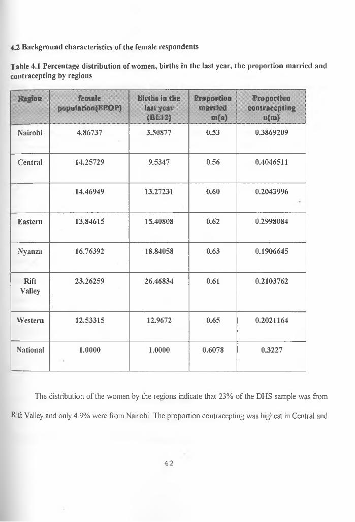
4.2 Background characteristics of the female respondents

Table 4.1 Percentage distribution of women, births in the last year, the proportion married and contracepting by regions

Region femalepopulation(FPOP)

births in the last year (BL12)

Proportionmarried

m(a)

Proportioncontracepting

u(m)

Nairobi 4.86737 3.50877 0.53 0.3869209

Central 14.25729 9.5347 0.56 0.4046511

14.46949 13.27231 0.60 0.2043996

Eastern 13.84615 15.40808 0.62 0.2998084

Nyanza 16.76392 18.84058 0.63 0.1906645

RiftValley

23.26259 26.46834 0.61 0.2103762

Western 12.53315 12.9672 0.65 0.2021164

National 1.0000 1.0000 0.6078 0.3227

The distribution of the women by the regions indicate that 23% of the DHS sample was from

Rift Valley and only 4.9% were from Nairobi. The proportion contracepting was highest in Central and

42

the least in Nyanza. The proportion married was highest in Western and least in Nairobi. Table 4.1

gives a summary of the characteristics by regions.

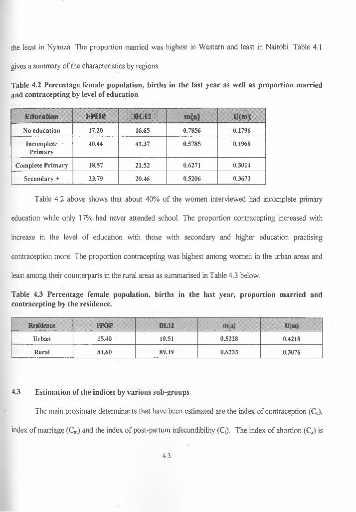
Table 4.2 Percentage female population, births in the last year as well as proportion married and contracepting by level of education

Education FPOP i m l i j m(a) U(m>

N o education 17.20 16.65 0.7856 0.1796

In com p lete • P rim ary

40.44 41.37 0.5785 0.1968

C om plete P rim ary 18.57 21.52 0.6271 0.3014

S econ d ary + 23.79 20.46 0.5206 0.3673

Table 4.2 above shows that about 40% of the women interviewed had incomplete primary

education while only 17% had never attended school. The proportion contracepting increased with

increase in the level of education with those with secondary and higher education practising

contraception more. The proportion contracepting was highest among women in the urban areas and

least among their counterparts in the rural areas as summarised in Table 4.3 below.

Table 4.3 Percentage female population, births in the last year, proportion married and contracepting by the residence.

R esidence FPO P BL 12

:: >»-v;

t '(m )

U rban 15.40 10.51 0.5228 0.4218

Rural 84.60 89.49 0.6233 0.3076

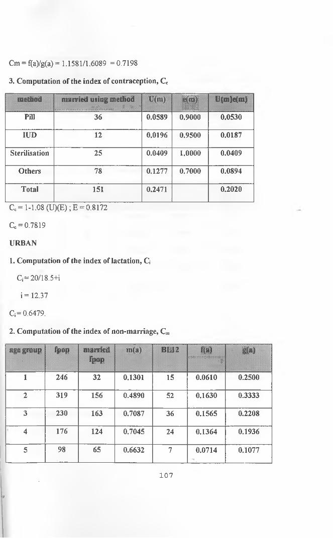
4.3 Estimation of the indices by various sub-groups

The main proximate determinants that have been estimated are the index of contraception (Cc),

index of marriage (Cm) and the index of post-partum infecundibility (Q). The index of abortion (Ca) is

43

not estimated in this study because its data is not easily available since abortion is an illegal practice in

Kenya.

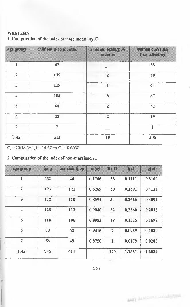
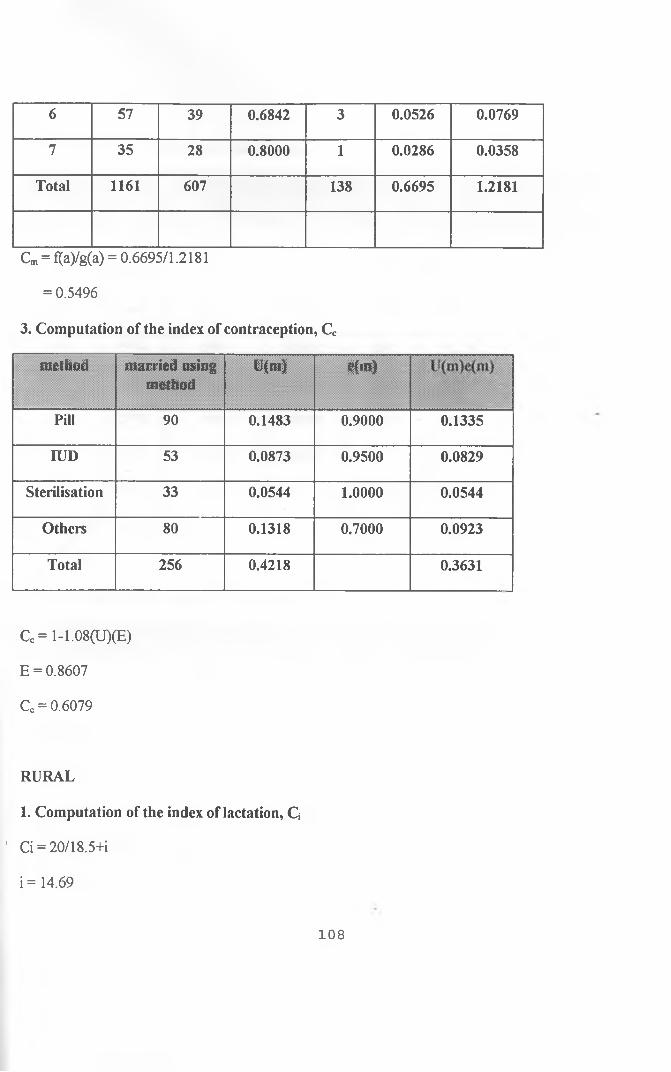
4.3.1 Estimation of the Index of Post-partum infecundibility (Q)

To compute the index of (Q), the duration of breast-feeding needs to be first estimated.

Breast-feeding is' a natural contraceptive whose mechanism is hormonal. Prolonged breast-feeding

lengthens the birth intervals due to its relationship with lactation amenorrhea, since for a great majority

of the women the ovaries are inactive for most of the period of lactation.

There are two methods of estimating the duration of breast-feeding. One is direct and-the other

is indirect. In the direct method breast-feeding duration is obtained by dividing the total number of

months women breast-feed in that sub-group by the total number of women in that sub-group.

However studies have shown that the direct method cannot yield accurate results since the data used

has errors in most cases. These errors include those caused by mis-reporting of the duration of breast­

feeding by the women interviewed. In this case some may under-report while others may over-report

their duration of breast-feeding. There also exists truncation error in this direct method of estimation.

This happens because during the time of interview, some respondents are still breast-feeding and hence

although the duration they have breast-fed so far is known, how much longer they will breast-feed is

not exactly known.

Finally, incompleteness of data is also a common source of error in the data collection.

44

Due to these unforeseen errors and problems, we found it necessary to use an indirect method to

estimate the duration of breast-feeding. A simple estimation procedure was chosen, the prevalence

incidence method, which gives us the desired mean duration of breast-feeding.

To obtain the mean duration of breast-feeding using the prevalence incidence method and hence the

index C*, the computational procedure will be given using the national level data.

Step 1 To compute the incidence (I)

I = l/36(all births 0-35 months before the survey +1/2 of births occurring 36 months prior to the

survey).

This gives the approximate number of births per month.

Step 2 Computation of the prevalence (P)

P = Number of children currently breast-feeding irrespective of age.

Step 3 Computation of the mean duration of breast-feeding

Mean duration of breast-feeding = Observed prevalence (P) /Average number of births per

month (P).

B = P/I

45

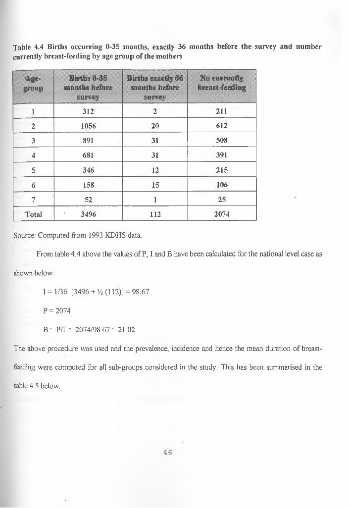
Table 4.4 Births occurring 0-35 months, exactly 36 months before the survey and number currently breast-feeding by age group of the mothers

Age-group

Births 0-35 months before

survey

Births exactly 36 months before

survey

No currently breast-feeding

1 312 2 211

2 1056 20 612

3 891 31 508

4 681 31 391

5 346 12 215

6 158 15 106

7 52 1 25

Total 3496 112 2074

Source: Computed from 1993 KDHS data.

From table 4.4 above the values of P, I and B have been calculated for the national level case as

shown below.

I = 1/36 [3496 + >/2 (112)] = 98.67

P = 2074

B = P/I = 2074/98.67 = 21.02

The above procedure was used and the prevalence, incidence and hence the mean duration of breast­

feeding were computed for all sub-groups considered in the study. This has been summarised in the

table 4.5 below.

46

Table 4.5 The prevalence, incidence and the mean duration of breast-feeding for all the sub­groups.

Sub-group Prevalence' <P>

Incidence(I)

Mean duration of breast-feeding (B)

National 2074 98.67 21.02

Nairobi 66 3.63 18.21

Central 204 10.68 19.11

Coast 263 12.68 20.74

Eastern 339 14.03 24.17

Nyanza 360 18.18 19.80

Rift Valley 536 25.04 21.40

Western 306 14.36 21.31

Urban 215 11.51 18.67

Rural 1859 87.15 21.33

No education 385 16.86 22.83

IncompletePrimary

840 40.83 20.57

CompletePrimary

429 20.3 21.11

Secondary + 420 20.65 20.34Computed from the 1993 KDHS data

Once the mean duration of breast-feeding has been estimated, then Ci is computed as follows.

Q = 20/(18.5+i)

where the i = 1.753e°lv9684)00187282 an(] b is the mean duration of breast-feeding.

For the national level case, the value of i was obtained to be 14.42 after substituting the value of

B = 21.02 into the equation for i.

47

Therefore:

C; = 20/ (18.5+14.42) = 20/32.92 = 0.6075

Using the same procedure as above, the index of post-partum infecundibilty was obtained for all sub­

groups. Table 4.6 below gives the Q values for all the sub-groups.

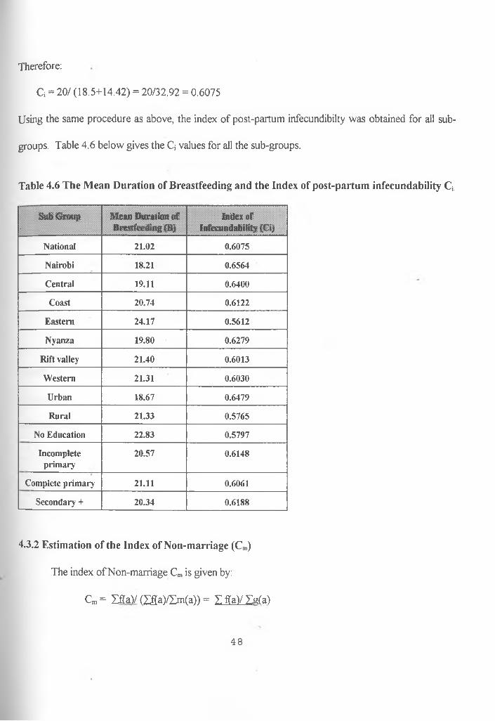
Table 4.6 The Mean Duration of Breastfeeding and the Index of post-partum infecundability Q

Sub Group.

M ean D uration o f Breastfeeding (B )

Index o fInfecundability (Ci)

National 21.02 0.6075

Nairobi 18.21 0.6564

Central 19.11 0.6400

Coast 20.74 0.6122

Eastern 24.17 0.5612

N yanza 19.80 0.6279

Rift valley 21.40 0.6013

W estern 21.31 0.6030

Urban 18.67 0.6479

Rural 21.33 0.5765

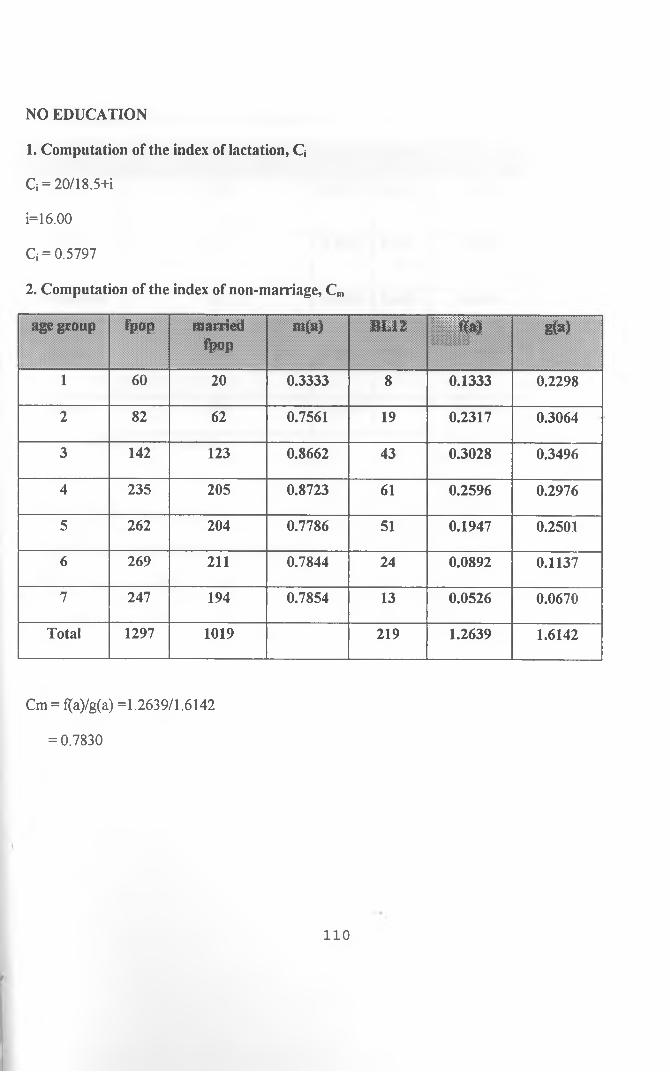
No Education 22.83 0.5797

Incom pleteprim ary

20.57 0.6148

C om plete prim ary 21.11 0.6061

Secondary + 20.34 0.6188

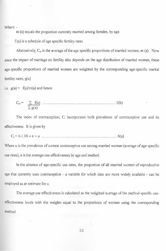
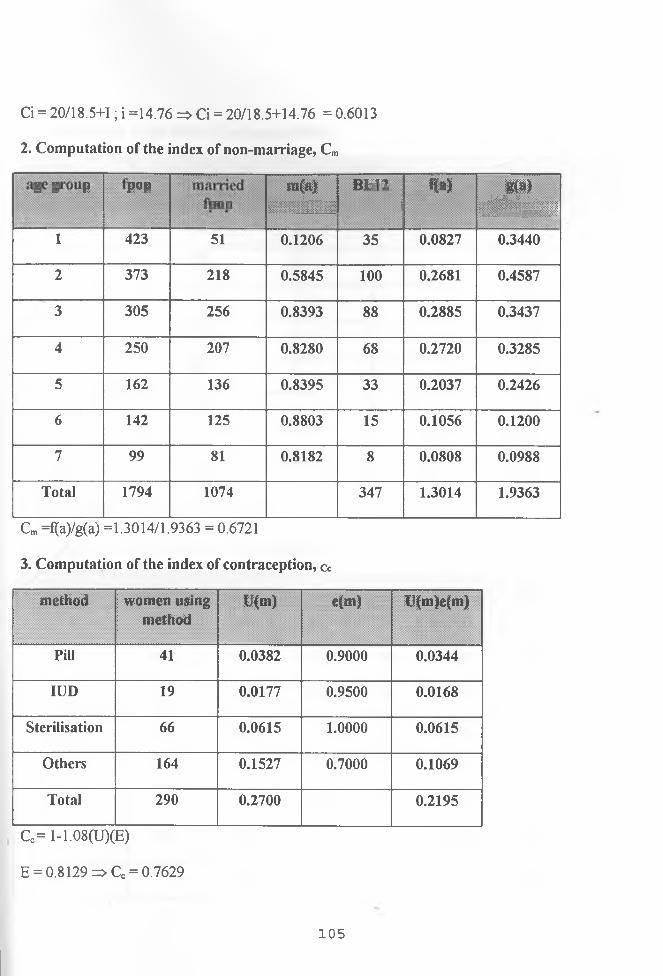
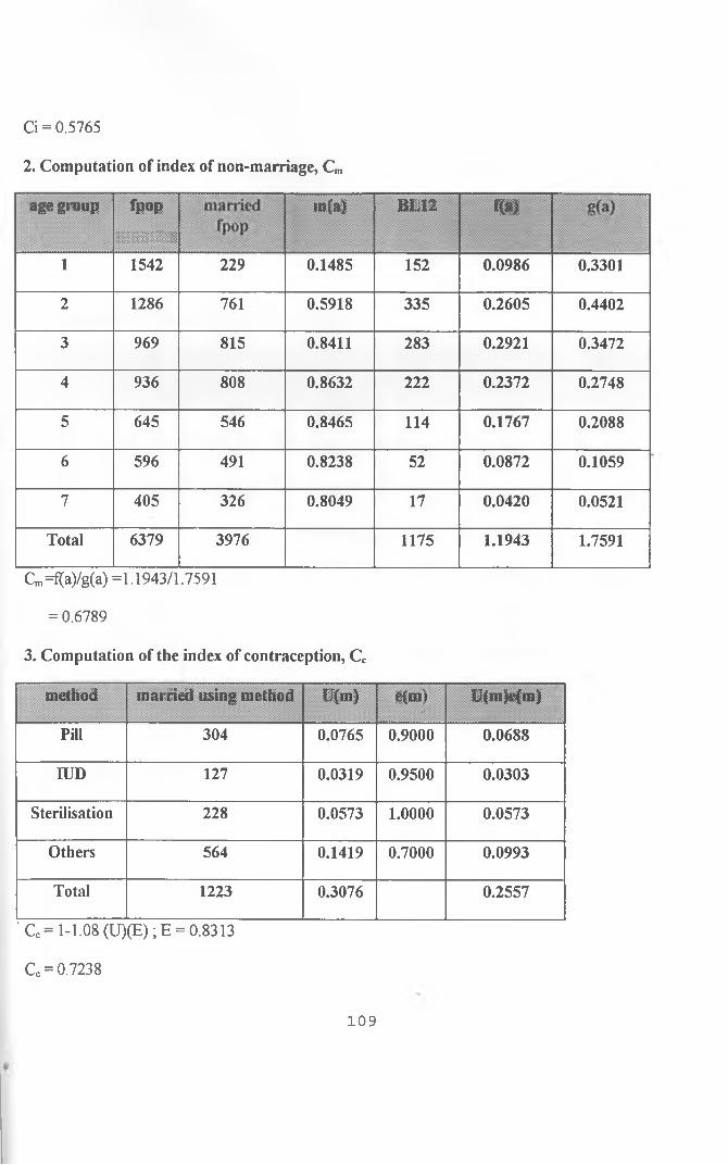
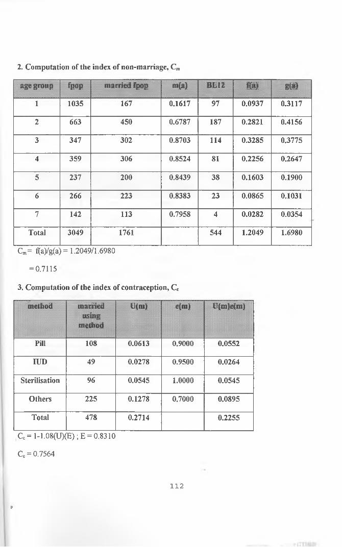
4.3.2 Estimation of the Index of Non-marriage (Cm)

The index of Non-marriage Cm is given by:

Cm = ZfTaV (Zfia)/Zm(a)) = I ffa)/ Zg(a)

48

Where:

L is sum of

f(a) is the age specific fertility rates obtained by dividing births in the last year by

female population in that particular age-group.

m(a) is the proportion married in a given age group obtained by dividing the married

women by the total female population in that age-group.

The ratio f(a)/m(a) is the age specific marital fertility rate denoted by g(a).

For the age-group 15-19, g(a) is estimated as:

g(15-19) = 0.75 x g(20-24)

The reason for this is because the direct estimate of g( 15-19) is unreliable especially where the value of

m(15-19) is very low as in most populations.

Hence the index of Non-marriage Cm is obtained by dividing the sum of all the age-specific

fertility rates Zf(a) by the sum of age-specific marital fertility rates Zg(a). Table 4.7 below gives a

summary of the required data for a national level case. The value of Cm is then obtained as in the

working below.

49

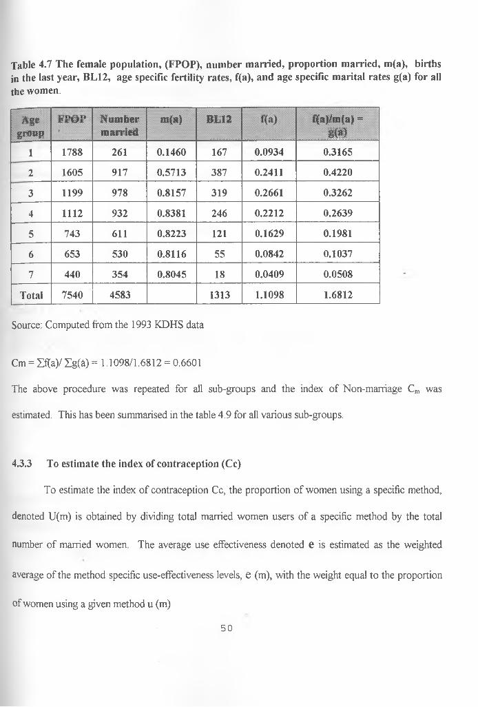
Table 4.7 The female population, (FPOP), number married, proportion married, m(a), births in the last year, BL12, age specific fertility rates, f(a), and age specific marital rates g(a) for all the women.

Agegroup

JT t U t

>

N um bermarried

m ( » ) BL12 f(a)/m(a) =m

1 1788 261 0.1460 167 0.0934 0.3165

2 1605 917 0.5713 387 0.2411 0.4220

3 1199 978 0.8157 319 0.2661 0.3262

4 1112 932 0.8381 246 0.2212 0.2639

5 743 611 0.8223 121 0.1629 0.1981

6 653 530 0.8116 55 0.0842 0.1037

7 440 354 0.8045 18 0.0409 0.0508

Total 7540 4583 1313 1.1098 1.6812

Source: Computed from the 1993 KDHS data

Cm = Zf(a)/ IgOO = 1.1098/1.6812 = 0.6601

The above procedure was repeated for all sub-groups and the index of Non-marriage Cm was

estimated. This has been summarised in the table 4.9 for all various sub-groups.

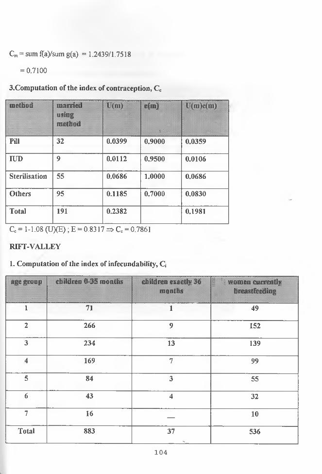
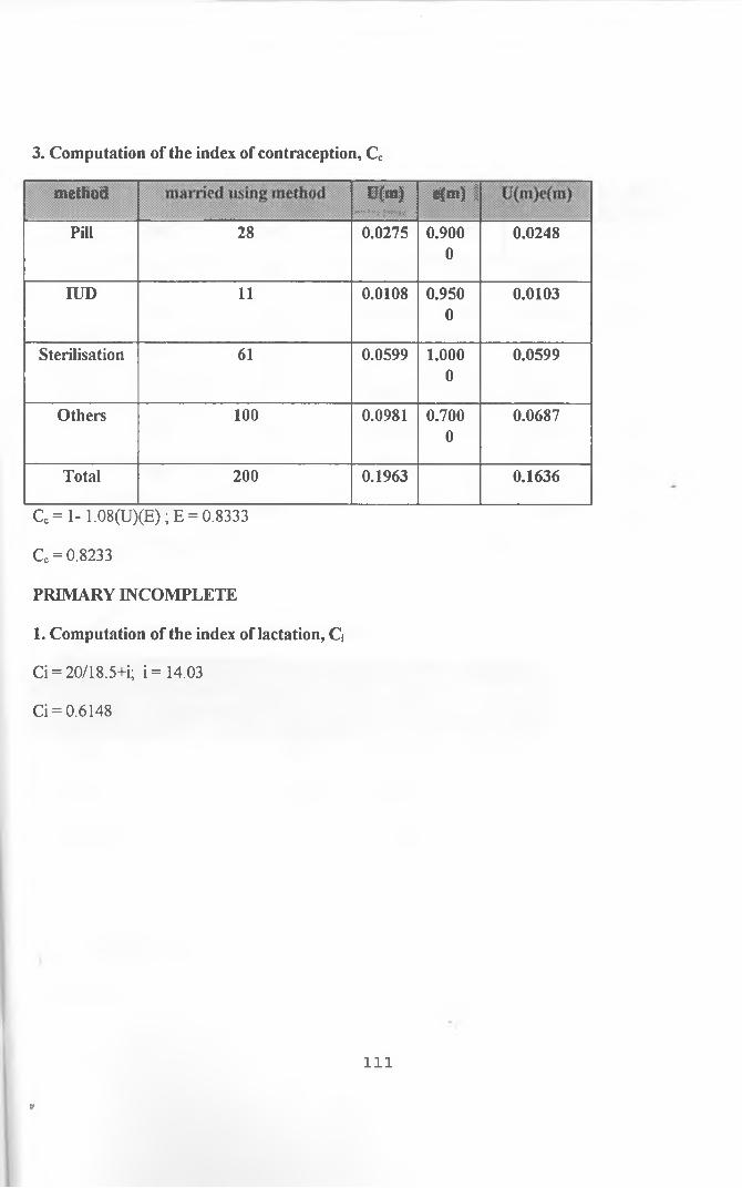
4.3.3 To estimate the index of contraception (Cc)

To estimate the index of contraception Cc, the proportion of women using a specific method,

denoted U(m) is obtained by dividing total married women users of a specific method by the total

number of married women. The average use effectiveness denoted e is estimated as the weighted

average of the method specific use-effectiveness levels, e (m), with the weight equal to the proportion

of women using a given method u (m)

50

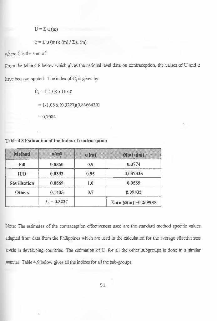
U = I u (m)

e = I u (m) e (m) / 1 u (m)

where E is the sum of

From the table 4.8 below which gives the national level data on contraception, the values of U and e

have been computed. The index of Cc is given by:

Ce = 1-1.08 x U x e

= 1-1.08 x (0.3227)(0.8366439)

= 0.7084

Table 4.8 Estimation of the Index of contraception

Method u(m) e(m ) e{m) u(m)

Pill 0.0860 0.9 0.0774

IUD 0.0393 0.95 0.037335

Sterilisation 0.0569 1.0 0.0569

Others 0.1405 0.7 0.09835

U = 0.3227 Eu(m)e(m) =0.269985

Note: The estimates of the contraception effectiveness used are the standard method specific values

adapted from data from the Philippines which are used in the calculation for the average effectiveness

levels in developing countries. The estimation of Cc for all the other subgroups is done in a similar

manner. Table 4.9 below gives all the indices for all the sub-groups.

51

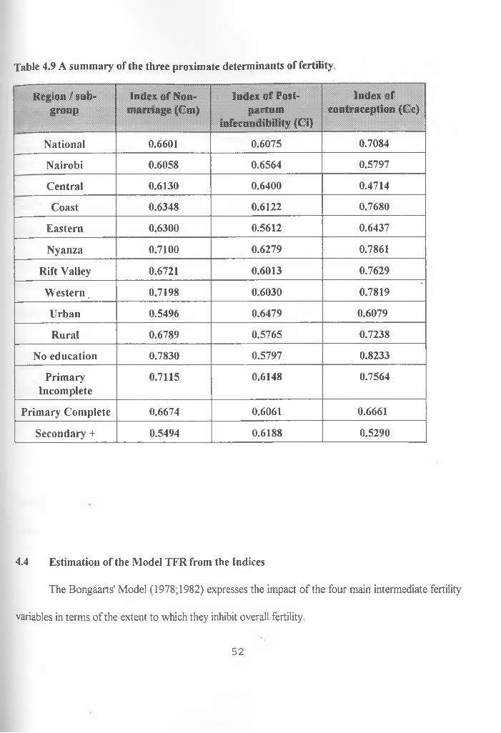
Table 4.9 A summary of the three proximate determinants of fertility.

R egion/sub­group

Index o f Non- m am age (Cm)

index of Post­partum

infecundibifity (Ci)

Index ofcontraception (Cc)

National 0.6601 0.6075 0.7084

Nairobi 0.6058 0.6564 0.5797

Central 0.6130 0.6400 0.4714

Coast 0.6348 0.6122 0.7680

Eastern 0.6300 0.5612 0.6437

Nyanza 0.7100 0.6279 0.7861

Rift Valley 0.6721 0.6013 0.7629

W estern, 0.7198 0.6030 0.7819

Urban 0.5496 0.6479 0.6079

Rural 0.6789 0.5765 0.7238

No education 0.7830 0.5797 0.8233

PrimaryIncomplete

0.7115 0.6148 0.7564

Primary Complete 0.6674 0.6061 0.6661

Secondary + 0.5494 0.6188 0.5290

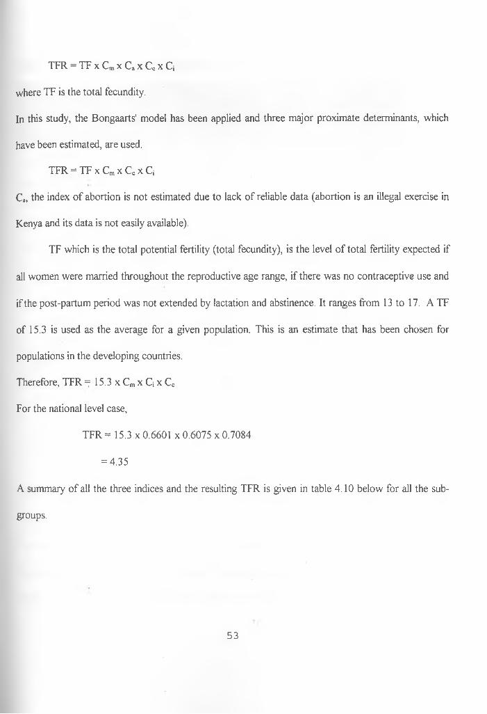
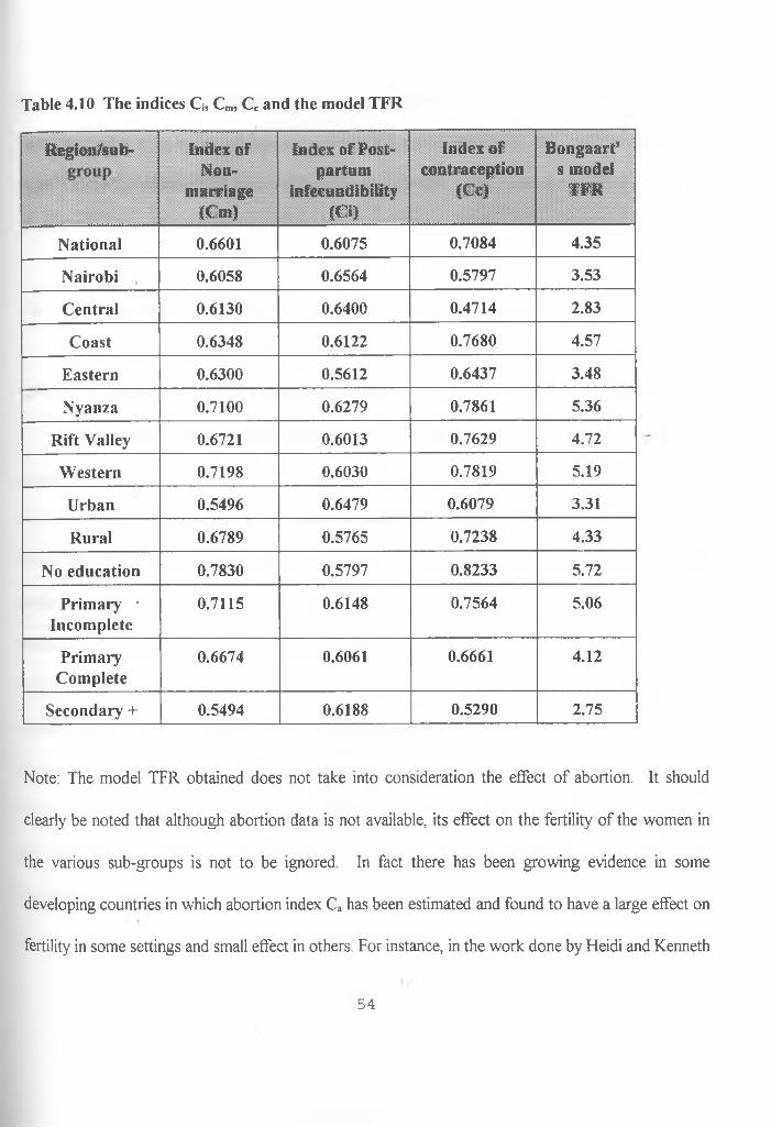
4.4 Estimation of the Model TFR from the Indices

The Bongaarts' Model (1978;1982) expresses the impact of the four main intermediate fertility

variables in terms of the extent to which they inhibit overall fertility.

52

TFR = TF X Cm X Ca X Cc X Ci

where TF is the total fecundity.

In this study, the Bongaarts' model has been applied and three major proximate determinants, which

have been estimated, are used.

TFR = TF x Cm x Cc x Ci

Ca, the index of abortion is not estimated due to lack of reliable data (abortion is an illegal exercise in

Kenya and its data is not easily available).

TF which is the total potential fertility (total fecundity), is the level of total fertility expected if

all women were married throughout the reproductive age range, if there was no contraceptive use and

if the post-partum period was not extended by lactation and abstinence. It ranges from 13 to 17. A TF

of 15.3 is used as the average for a given population. This is an estimate that has been chosen for

populations in the developing countries.

Therefore, TFR = 15.3 x Cm x Cj x Cc

For the national level case,

TFR = 15.3 x 0.6601 x 0.6075 x 0.7084

= 4.35

A summary of all the three indices and the resulting TFR is given in table 4.10 below for all the sub­

groups.

53

Table 4.10 The indices Q, Cm, Cc and the model TFR

Region/sub- Index of Non-

marriage (Cm)

Index of Post­partum

infecundibility (Ci)

Index of contraception

(Cc)

Bongaart’ s model

TER

National 0.6601 0.6075 0.7084 4.35

Nairobi 0.6058 0.6564 0.5797 3.53

Central 0.6130 0.6400 0.4714 2.83

Coast 0.6348 0.6122 0.7680 4.57

Eastern 0.6300 0.5612 0.6437 3.48

Nyanza 0.7100 0.6279 0.7861 5.36

Rift Valley 0.6721 0.6013 0.7629 4.72

Western 0.7198 0.6030 0.7819 5.19

Urban 0.5496 0.6479 0.6079 3.31

Rural 0.6789 0.5765 0.7238 4.33

No education 0.7830 0.5797 0.8233 5.72

Primary ■ Incomplete

0.7115 0.6148 0.7564 5.06

PrimaryComplete

0.6674 0.6061 0.6661 4.12

Secondary + 0.5494 0.6188 0.5290 2.75

Note: The model TFR obtained does not take into consideration the effect of abortion. It should

clearly be noted that although abortion data is not available, its effect on the fertility of the women in

the various sub-groups is not to be ignored. In fact there has been growing evidence in some

developing countries in which abortion index Ca has been estimated and found to have a large effect on

fertility in some settings and small effect in others. For instance, in the work done by Fleidi and Kenneth

54

(1996) on induced abortion in developing world, the estimate for abortion index between the period

1988-1989 was 1.011, but this decreased to 0.748 during the period 1993. This clearly indicates that

there has been increasing effects of abortion (induced) on fertility in the recent past, a factor that cannot

go unmentioned in this analysis.

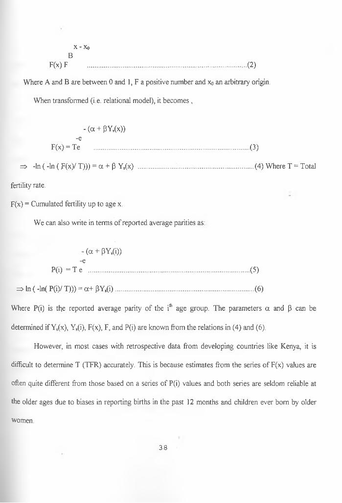
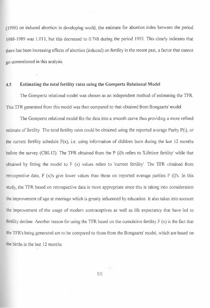
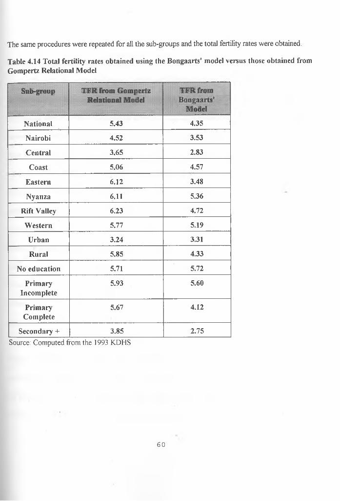
4.5 Estimating the total fertility rates using the Gompertz Relational Model

The Gompertz relational model was chosen as an independent method of estimating the TFR.

This TFR generated from this model was then compared to that obtained from Bongaarts' model.

The Gompertz relational model fits the data into a smooth curve thus providing a more refined

estimate of fertility. The total fertility rates could be obtained using the reported average Parity P(i), or

the current fertility schedule F(x), i.e. using information of children bom during the last 12 months

before the survey (CBL12). The TFR obtained from the P (i)'s refers to lifetim e fertility' while that

obtained by fitting the model to F (x) values refers to 'current fertility'. The TFR obtained from

retrospective data, F (x)'s give lower values than those on reported average parities P (i)'s. In this

study, the TFR based on retrospective data is more appropriate since this is taking into consideration

the improvement of age at marriage which is greatly influenced by education. It also takes into account

the improvement of the usage of modem contraceptives as well as life expectancy that have led to

fertility decline. Another reason for using the TFR based on the cumulative fertility F (x) is the fact that

the TFR's being generated are to be compared to those from the Bongaarts' model, which are based on

the births in the last 12 months.

55

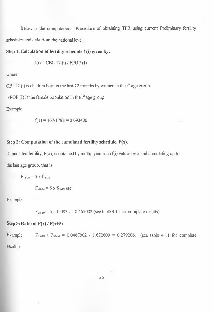
Below is the computational Procedure of obtaining TFR using current Preliminary fertility

schedules and data from the national level.

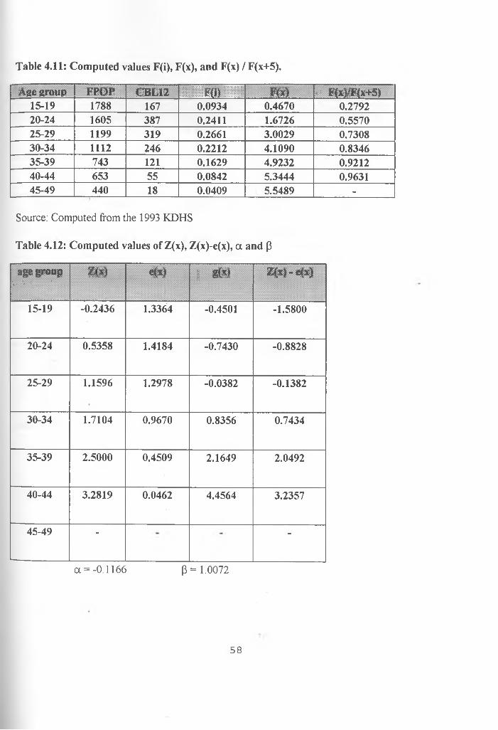
Step 1: Calculation of fertility schedule f (i) given by:

f(i) = CBL 12 (i)/FPOP (I)

where

CBL12 (i) is children bom in the last 12 months by women in the iu’ age group

FPOP (I) is the female population in the i* age group

Example:

f(l) = 167/1788 = 0.093400

Step 2: Computation of the cumulated fertility schedule, F(x).

Cumulated fertility, F(x), is obtained by multiplying each f(i) values by 5 and cumulating up to

the last age group, that is

F15-19 = 5 X f)5-l9

F20-24 = 5 x fi5-i9 etc.

Example:

F15-19 = 5 x 0.0934 = 0.467002 (see table 4.11 for complete results).

Step 3: Ratio of F(x) / F(x+5)

Example: F15.19 / F20-24 = 0.0467002 / 1.672609 = 0.279206. (see table 4.11 for complete

results).

56

Step 4: Z(x) = -In [-In (F(x) / F(x+5))]

Example: Z15.i9 = -In [-In (0.279206)] = -0.243578

Step 5: Z(x) - e(x) =Yj.......(see table 4.12)

Step 6: Computation of YA(x)

Y'Xx) = a +PYs(x)

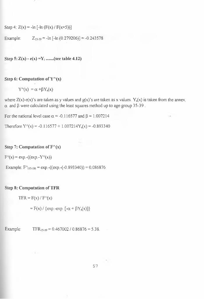
where Z(x)-e(x)’s are taken as y values and g(x)’s are taken as x values. Ys(x) is taken from the annex, a and (3 were calculated using the least squares method up to age group 35-39 .

For the national level case a = -0.116577 and P = 1.007214

Therefore YA(x) = -0.116577 + 1,007214Ys(x) = -0.893340

Step 7: Computation of FA(x)

F'Xx) = exp.-((exp.-YA(x))

Example: FAi5.i9) = exp.-((exp.-(-0.893340)) = 0.086876

Step 8: Computation of TFR

TFR = F(x) / FA(x)

= F(x) / {exp.-exp. [-a + PYs(x)]}

Example: TFR15-i9 = 0.467002 / 0.86876 = 5.38.

57

Table 4.11: Computed values F(i), F(x), and F(x) / F(x+5).

Age group FPOP CBL12 wmmwm m * = FfxVF(x+5)15-19 1788 167 0.0934 0.4670 0.279220-24 1605 387 0.2411 1.6726 0.557025-29 1199 319 0.2661 3.0029 0.730830-34 1112 246 0.2212 4.1090 0.834635-39 743 121 0.1629 4.9232 0.921240-44 653 55 0.0842 5.3444 0.963145-49 440 18 0.0409 5.5489 -

Source: Computed from the 1993 KDHS

Table 4.12: Computed values of Z(x), Z(x)-e(x), a and P

age group* %• * ' * •

m <**) : s m Z <*)-e(x)

15-19 -0.2436 1.3364 -0.4501 -1.5800

20-24 0.5358 1.4184 -0.7430 -0.8828

25-29 1.1596 1.2978 -0.0382 -0.1382

30-34 1.7104 0.9670 0.8356 0.7434

35-39 2.5000 0.4509 2.1649 2.0492

40-44 3.2819 0.0462 4.4564 3.2357

45-49'

“

a = -0.1166 p= 1.0072

58

Table 4.13: Computed values of AY(x), AF(x) and TFR.

Age gro«l> Ys(*)wmtmsm • -

T F R

15-19 -0 .7 7 1 2 -0 .8 9 3 4 0 .0 8 6 9 5 .38

20-24 -0 .0 4 1 0 -0 .1 5 7 9 0 .3 1 0 0 8 .39

25-29 0 .6 2 9 4 0 .5 1 7 4 0 .5 5 1 0 5 .45

30-34 1 .8878 1.2881 0 .4 5 5 0 5 .43

3 4-39 2 .4 7 3 6 2 .3 7 4 9 0 .9 1 1 2 5 .4 0

40-44 4 .4 9 8 4 4 .4 1 4 2 0 .9 8 8 0 5.41

45-49 9 .3 4 1 6 9 .2 9 2 4 0.9991 5 .5 5

Mean total fertility rate is 5.43

59

The same procedures were repeated for all the sub-groups and the total fertility rates were obtained.

Table 4.14 Total fertility rates obtained using the Bongaarts' model versus those obtained from Gompertz Relational Model

Sub-group TER from Gompertz Relational Model

TFR from

Model

National 5.43 4.35

Nairobi 4.52 3.53

Central 3.65 2.83

Coast 5.06 4.57

Eastern 6.12 3.48

Nyanza 6.11 5.36

Rift Valley 6.23 4.72

Western 5.77 5.19

Urban 3.24 3.31

Rural 5.85 4.33

No education 5.71 5.72

PrimaryIncomplete

5.93 5.60

PrimaryComplete

5.67 4.12

Secondary + 3.85 2.75Source: Computed from the 1993 KDHS

60

4.6 Comparing the TFR’S estimated from Bongaart’s model with those estimated from the

Gompertz relational model.

The table above gives a summary of the total fertility rates obtained using the Gompertz

relational model and the Bongaarts' model. The difference between the two fertility rates range from

0.01 among women with no education, to 2.64 for women from eastern province. The mean difference

however is 0.989 births per woman. It can however be deduced that apart from a few cases of women

from eastern, rift valley, rural areas and among those with primary complete education, the fertility

rates are not very different. For eastern province, the Bongaarts' TFR is 3.48, far much lower than the

Gompertz TFR. This may be due to its low index of contraception and index of post-partum

infecundability of 0.6437 and 0.5612 respectively. The observed level of contraception at the time of

the survey may not have had its full effect on fertility due to lag effects. Another reason for this low

fertility rate could be reporting errors by the respondents during the time of survey. Therefore although

this same province had the lowest level of Q of 0.6160 in 1989, the drop from 0.6160 to 0.5612 of

about 9 percent may not have actually occurred. Similarly a drop from 0.80796 to 0.6437 in the index

of lactation, Cc, which is equivalent to an increase of 20.3% in the use of contraception may also not

have occurred.

On the other hand, the Gompertz relational model may not be able to reflect sufficiently on

changes that affect the proximate determinants of fertility. For example, the Gompertz model uses data

on the births in the last 12 months while Cc is determined by the current users of contraception during

the time of the survey. It should be noted that births in the last year is affected by the level of usage

prior to the survey and not by the number of users during the survey. This may be summarised as the

61

by effects in which the current use of contraceptives only determines future fertility and not current

fertility. The low value of Q of 0.5612 is due to a long duration of breast-feeding of 24.17 for eastern

province, which is the longest duration among all the regions. This was also the case in 1989

(Wamalwa, 1991). However, although there is some consistency, we cannot rule out errors in

reporting of the data used to estimate the mean duration of breast-feeding as well as the proportion

contracepting in this province.

The other difference in the other values of TFR for the other various sub-groups may be

attributed to the methodology differences. The use of a TFR of 15.3 is only an agreed on standard

which may not be true for all the sub-groups. The effects of other proximate determinants e.g.- index of

abortion, Ca and index of sterility cannot be ignored. In fact there is evidence that the secondary and

primary sterility is on the decrease which may in turn lead to an increase in fertility which cannot be

explained by the two models being used. Abortion is also playing a crucial role in reducing fertility in

the recent past and this too has not been taken into account when the model TFR was estimated.

Where the total fecundity has been under-estimated, this has the effect of lowering the total fertility

rate. Thus the TFR's estimated from Bongaarts' model are generally lower than those estimated from

Gompertz relational model. This may have been as a result of under-estimating the total fecundity rate.

4,7 Estimating the role of each proximate determinant in reducing fertility

In this section, the attempt is to uncover the mechanisms that are at play in producing current

overall levels of fertility and to assess the relative role of each of the intermediate variables to overall

62

fertility levels. A further attempt is also made to examine the combined effect of these variables on

fertility in Kenya.

In section 4.3, the Bongaarts' Model was chosen to estimate the indices of the three proximate

determinants of fertility. The model expresses the impact of each of the three intermediate variables of

fertility in terms of the extent to which it inhibits overall fertility. These indices take the values 0-1 and

the greater the fertility-inhibiting effect of a given variable, the lower the value. Thus the indices take

the value of 1 when the determinant has no effect on fertility and the value 0 when the determinant

eliminates all fertility, a situation which is not at all practical.

Table 4.15 The Indices of Non-marriage, Lactation and Contraception at the National level

C m Q , Q TFR(Bongaarts')

0.6601 0.6075 0.7084 4.35

From Table 4.15, it can be deduced that the index of lactation is the lowest, while that of

contraception is the highest. The implication here is that fertility reducing effect of lactation is greater

than that of the other two and that fertility-inhibiting effect of contraception is the lowest. This was the

same finding by Wamalwa (1991). According to him, the index of lactation was 0.6356, that of non­

marriage was 0.7353 and that of contraception was 0.8216. Thus the index of lactation had the greatest

fertility inhibiting effect, followed by non-marriage then contraception.

63

Table 4.16 The Indices of Non-marriage, Lactation and Contraception among women by the 7 provinces

Region Cm O . ' c , • TFR (1993) TFR (1989)

Nairobi 0.6058 0.6564 0.5797 3.53 4.51

Central 0.6130 0.6400 0.4714 2.83 5.97

Coast 0.6348 0.6122 0.7680 4.57 5.64

Eastern 0.6300 0.5612 0.6437 3.48 6.42

Nyanza 0.7100 0.6279 0.7861 5.36 7.08

RiftValley

0.6721 0.6013 0.7629 4.72 6.66

Western 0.7198 0.6030 0.7819 5.19 8.10

Source: (1) Computed from KDHS 1993

(2) Wamalwa 1991

From Table 4.16, it can be deduced that non-marriage has the greatest inhibiting effect in

Nairobi province and least impact of fertility in Western province. Lactation on the other hand has the

greater impact on fertility in Eastern province and the least impact in Nairobi. Central province has the

lowest index of contraception while Western has the highest. Thus reducing effect on contraception on

fertility is greater in Central province and least in Western province. Nairobi, Central and Eastern

provinces can be said to be regions of low fertility (less than 4.0) while coast and Rift valley provinces

may be said to be regions of moderate fertility (between 4.0 and 5.0). Nyanza and Western provinces

with very high TFR are regions of high fertility (more than 5.0). Central province has the lowest total

fertility rate while Nyanza province has the highest.

The scenario above seems to have slightly changed between the period 1989 to 1993. Eastern

province seems to have switched positions with Coast province which is now a region of moderate

64

fertility while the former is a region of low fertility. This may be attributed to the long breast-feeding

periods and increased use of contraceptives in eastern province than in the Coast province. Western

and Nyanza provinces are still regions of high fertility. We can further deduce from the table that the

three proximate determinants of fertility have played a great role in reducing fertility in all the regions of

Kenya. The greatest reduction was achieved in central province (approximately 3 births) and least in

Nairobi province (1 birth). On average, these fertility inhibiting variables reduced fertility during the

periods 1989 and 1993 by about 2 births among the regions of Kenya.

As a result of these variations on effect at the regional level, we can say that the only index that

has maintained the same position at the regional level is that of non-marriage. It is the second most

important fertility inhibiting variable. Contraception and lactation are seen to switch positions with the

latter being the most important fertility-inhibiting variable in five of the seven regions and the former in

only two regions.

When we contrast this picture with that at the national level, we find that lactation has the

greatest influence on fertility in these five regions namely Eastern, Coast, Rift valley, Western and

Nyanza. In these regions also non-marriage comes second in importance in influencing fertility, with

contraception being the least important. This agrees strongly with the general picture at the national

level. However Nairobi and Central regions have a different pattern altogether. Contraception is the

most important variable influencing fertility followed by non-marriage then lactation. This may be due

to high levels of education in these regions as well as urbanisation that both favour the use of

contraceptives as well as delayed marriages.

65

Table 4.17 The Indices of Non-marriage, Lactation and Contraception among women by levelsof education

Education Level CM G G TFR

No education 0.7830 0.5797 0.8233 5.72

PrimaryIncomplete

0.7115 0.6148 0.7594 5.06

PrimaryComplete

0.6674 0.6061 0.6661 4.12

Secondary + 0.5494 0.6188 0.5290 2.75

From Table 4.17 it is clear that the Index of Non-marriage decreases with increases in

education such that the inhibiting effect of non-marriage is highest among women with secondary and

higher education and lowest among those with no education. The effect of lactation on reducing

fertility is vice versa; greatest among women with no education and lowest among women with

secondary and higher level of education. For contraception, the index is lowest among women with

secondary and higher education and highest among those with no education. Thus the inhibiting effect

of contraception is highest among the highly educated and lowest among those with little or no

education. The TFR computed from these indices varies inversely with the level of education such that

the higher the level of education the lower the level of fertility.

Table 4.18 The Indices of Non-marriage, Lactation and Contraception among women in the rural and urban areas

Residence C* . c t Cc TFR

Urban 0.5496 0.6479 0.6079 3.31

Rural 0.6789 0.5765 0.7238 4.33From Table 4.18, it is evident that women residing in the urban areas have a lower index of

non-marriage and contraception than their counterparts in the rural areas. This implies that the index of

66

non-marriage and contraception has a greater impact on reducing fertility among women in the urban

areas than those living in the rural areas. The women in the rural areas however have the lowest index

of lactation than those in the urban areas. Thus fertility reducing effect of lactation is greatest among

women in the rural areas than those in the urban areas. These fertility-inhibiting factors have a greater

impact on fertility among the women in the urban areas than those in the rural areas.

4.8 The impact of Proximate Determinants of fertility on fertility using the percentage

reduction in fertility

To be able to estimate the percent reduction in fertility as a result of the inhibiting effect of the

proximate determinants, we first use the Bongaarts' model to estimate the total natural marital fertility

(TN), the total marital fertility (TM) and the total fertility rate (TFR).

The total natural marital fertility (TN) is given by TF x Q. This measures the effect of lactation on

fertility, which is, given by the difference between C (Total fecundity) and TN where C is 15.3. The

percentage reduction in fertility due to lactation is then given by:

(C- TN) /C x 100

The values of C, TN, (C-TN) and the percentage reduction in fertility are given in Table 4.19 below.

67

Table 4.19 The values of C, TN and C-TN and the percent reduction of fertility due to lactationby regions

Region C<

■ TN - C X O C-TN •>s i w S i v s

% *.

percent Reduction in

Fertility

Nairobi 15.3 10.0 5.3 34.6

Central 15.3 9.79 5.51 36.0

Coast 15.3 9.37 5.93 38.8

Eastern 15.3 8.59 6.71 43.9

Nyanza 15.3 9.61 5.69 37.2

Rift Valley 15.3 9.20 6.10 39.9

Western 15.3 9.23 6.07 39.7

National 15.3 9.29 6.01 39.3

The effect of lactation on fertility can be established by obtaining the difference between the

total fecundity rate and the natural fertility rate. The bigger the difference, the greater the reduction in

fertility and hence the greater the impact of lactation on fertility. Therefore from Table 4.19, lactation

has the greatest impact on fertility in Eastern province where the percent reduction in fertility is 43.9

and least in Nairobi where reduction was 34.6 percent.

68

Table 4.20 The values of C, TN C-TN and the percent reduction in fertility among women bylevels of education

EducationLevel

C T N ~ C * ans' jgj . s

C-TN percent Ikeduction In , : fe r tility

NoEducation

15.3 8.87 6.43 42.0

PrimaryIncomplete

15.3 9.41 5.89 38.5

PrimaryComplete

15.3 9.27 6.03 39.4

Secondary + 15.3 9.47 5.83 38.1

From Table 4.20 it is indicative that the higher the level of education, the lower the percent

reduction in fertility due to lactation. Thus the impact of lactation on fertility reduces as the level of

education among women increases. However, it should be noted that the difference in percent

reduction of fertility due to lactation among primary incomplete and primary complete slightly varies

from this trend. Women with primary complete education seem to lactate longer than those with

primary incomplete.

There also exists a notable difference in the impact of lactation on fertility among women

residing in urban areas and those residing in rural areas. Table 4.21 below indicates that the greatest

percent reduction in fertility is among women in the rural areas than those in the urban areas which in

turn implies a greater impact of lactation on fertility among these women than their counterparts in the

urban areas.

69

Table 4.21 The values of C, TN, C-TN and the percent reduction in fertility among women inrural and urban areas.

Residence c T N * C x C l C-TN percent Reduction in fertility

Urban 15.3 9.91 5.39 35.2

Rural 15.3 8.82 6.48 42.4

The percentage reduction in fertility due to Lactation at the national level is 39.3.

The total marital .fertility (TM) is given by Cc x TN. This in turn measures the effect of contraception

on fertility (abortion being assumed to be negligible in Kenya). The percentage reduction in fertility due

to contraception is given by

(TN-TM) / TN x 100

Table 4.22 Values of TN, TM, TN - TM and the percent Reduction in fertility due to contraception by provinces

Region TN TM TN-TM percent Reduction in fertility

Nairobi 10.0 5.82 4.22 42.0

Central 9.79 4.62 5.18 52.9

Coast 9.37 7.19 2.17 23.2

Eastern 8.59 5.53 3.06 35.6

Nyanza 9.61 7.55 2.05 21.4

Rift Valley 9.20 7.02 2.18 23.7

Western 9.23 7.21 2.01 21.8

National 9.29 6.58 2.71 29.2

70

From Table 4.22 it is evident that the impact of contraception on fertility is greatest in Central

Province and the least in Western Province. This is because the difference in

TN - TM is greatest in Central Province and smallest in Western. This in turn gives rise to a percent

reduction in fertility of 52.9 and 21.8 respectively.

Table 4.23 TN, TM, TN - TM values and the percent reduction of fertility among women by levels of education and place of residence.

Education . TN TM TN - TM Percent reduction in fertility

No education 8.87 7.30 1.57 17.7Primary

incomplete9.41 7.12 2.29 24.3

Primarycomplete

9.27 6.18 3.09 33.3

Secondary + 9.47 5.01 4.46 47.1Urban 9.91 6.03 3.88 39.2Rural 8.82 6.38 2.44 27.7

Table 4.23 reflects that the difference between TN and TM increases with the level in

education. The impact of contraception on fertility therefore increases with the increase in the level of

education. This phenomenon is seen to happen very consistently. There is a distinct difference in the

impact of contraception among women residing in rural and urban areas. The greatest impact of

contraception on fertility is marked among the women in the urban areas and least among their

counterparts in the rural areas.

The percentage reduction in fertility due to contraception at the national level is 29.2. The total

fertility rate (TFR) is given by Cm xTM, where Cm is the index of Non-marriage. The difference

between TM and TFR is the impact of Non-marriage on fertility patterns. The percentage reduction on

fertility due to Non-marriage is given by (TM - TFR) / TM x 100

71

Table 4.24 TM, TFR, TM - TFR Values and the % Reduction in fertility among women byregions

Region TM TFR TM - TFR % Reduction in fertility

Nairobi 5.82 3.53 2.29 39.3

Central 4.62 2.83 1.79 38.7

Coast 7.19 4.57 2.62 36.4

Eastern 5.53 3.48 2.05 37.1

Nyanza 7.55 5.36 2.19 29.0

Rift Valley 7.02 4.72 2.30 32.8

Western 7.21 5.19 2.02 28.0

National 6.58 4.34 2.24 34.0

From table 4.24 above, Nairobi province has the greatest percent reduction in fertility due to

non-marriage and the smallest percent reduction is found in western province. Thus the impact of non­

marriage is greatest in Nairobi and least among women in western province. As for women with

different levels of education, the impact of non-marriage is greatest among those with secondary and

higher level of education and least among those with no education. In fact the impact of non-marriage

on fertility increases with the increase in the level of education.

72

Table 4.25 TM, I KK, TM - TFR Values and the % Reduction in fertility among women byeducation levels and place of residence.

Education/Residence TM TFR TM - TFR % Reduction in fertility

No Education 7.30 5.72 1.58 21.6

Primary Incomplete 7.12 5.06 2.06 28.9

Primary Complete 6.18 4.12 2.06 33.3

Secondary + 5.01 2.75 2.26 45.1

Urban 6.03 3.31 2.72 45.1

Rural 6.38 4.33 2.05 32.1

As with women in different residential areas, it can be said from table 4.25 below that the

impact of non-marriage is greatest among those in urban areas and smallest among those in the rural

areas. At the national level, the percentage reduction in fertility due to non-marriage is 34.

From the above analysis, it can be deduced that the greatest fertility inhibiting factor is post­

partum infecundability which reduces the total fecundity at the national level by 39.3 percent followed

by the reducing effect of non-marriage (34.0 percent). The least fertility-inhibiting factor at the national

level is contraception, whose overall percentage reduction in fertility is 29.2 percent. This agrees with

Wamalwa's findings (1991) that contraception was the least fertility inhibiting variable with a percent

reduction of 18 while non-marriage was the second important variable with a percent reduction in

fertility of 26 and lactation being the most important of the three with a percent reduction in fertility of

36. However, a keen look at contribution of each proximate determinant between the period 1989-

1993 reveals a different situation altogether.

73

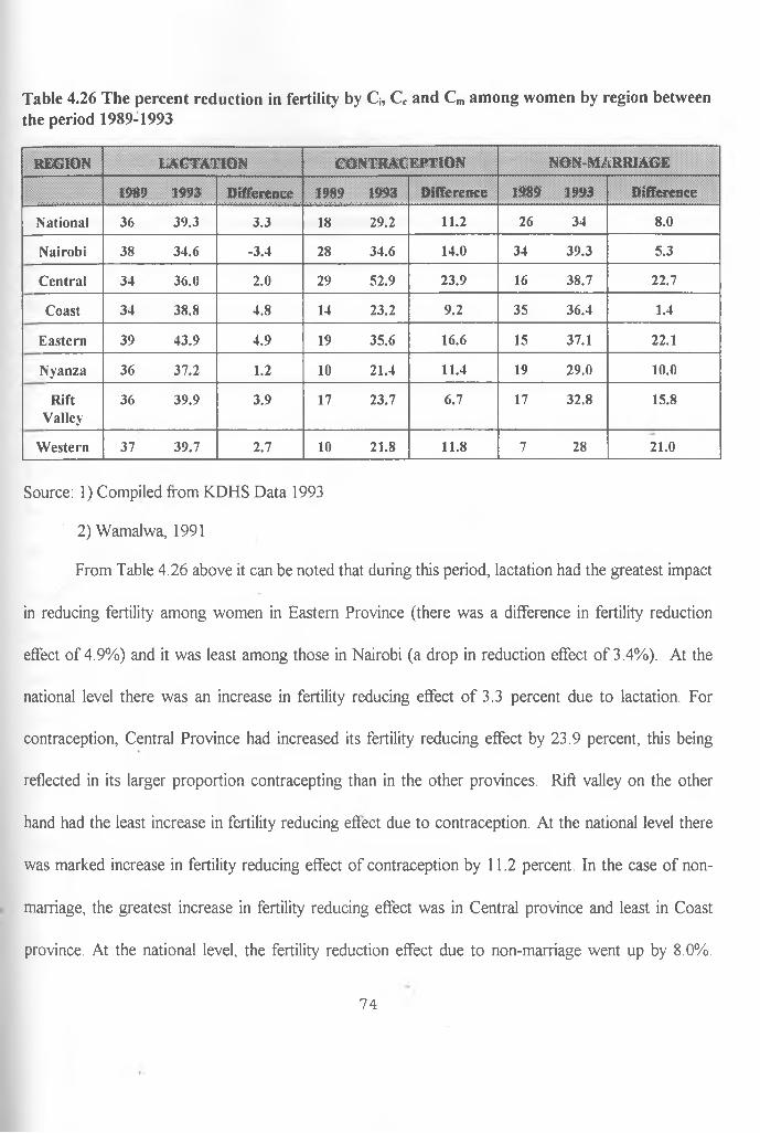
Table 4.26 The percent reduction in fertility by Ci5 Cc and Cm among women by region betweenthe period 1989-1993

R EG IO N L A C T A T IO N C O N T R A C E P T IO N N O N -M A R R IA G E

1989 1993 D iffe re n c e 1989 1993 D ifferen ce 1989 1993 D ifferen ce

N ational 36 39 .3 3.3 18 29.2 11.2 26 34 8.0

N airob i 38 34 .6 -3 .4 28 34.6 14.0 34 39 .3 5.3

C entral 34 36.0 2.0 29 52.9 23.9 16 38 .7 22.7

C oast 34 38.8 4.8 14 23.2 9.2 35 36.4 1.4

E astern 39 43 .9 4 .9 19 35.6 16.6 15 37.1 22.1

N yanza 36 37 .2 1.2 10 21.4 11.4 19 29.0 10.0

R iftV alley

36 39 .9 3.9 17 23.7 6 .7 17 32.8 15.8

W estern 37 39.7 2.7 10 21.8 11.8 7 28 21.0

Source: 1) Compiled from KDHS Data 1993

2) Wamalwa, 1991

From Table 4.26 above it can be noted that during this period, lactation had the greatest impact

in reducing fertility among women in Eastern Province (there was a difference in fertility reduction

effect of 4.9%) and it was least among those in Nairobi (a drop in reduction effect of 3.4%). At the

national level there was an increase in fertility reducing effect of 3.3 percent due to lactation. For

contraception, Central Province had increased its fertility reducing effect by 23.9 percent, this being

reflected in its larger proportion contracepting than in the other provinces. Rift valley on the other

hand had the least increase in fertility reducing effect due to contraception. At the national level there

was marked increase in fertility reducing effect of contraception by 11.2 percent. In the case of non­

marriage, the greatest increase in fertility reducing effect was in Central province and least in Coast

province. At the national level, the fertility reduction effect due to non-marriage went up by 8.0%.

74

Therefore considering the three proximate determinants during this period, it can be said that

contraception had the greatest fertility inhibiting effect of 11 .2 percent, followed by non-marriage with

8.0 percent and then lactation with 3.3 percent. Thus fertility inhibiting effect of contraception has been

greater than that of the other two proximate determinants in the few years preceding the 1993 KDHS

survey, a fact that agrees with other findings related to the transition to lower fertility in Kenya (Cross

R., Walter Obungu and Paul Kizito, 1991; National Research Council, 1993).

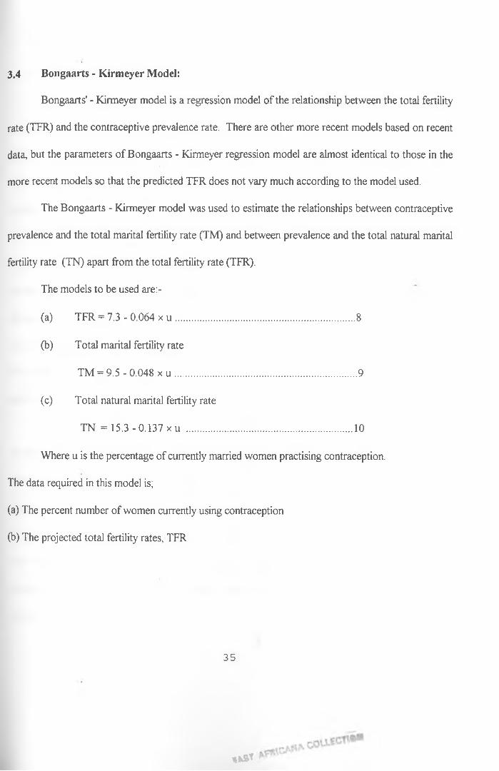
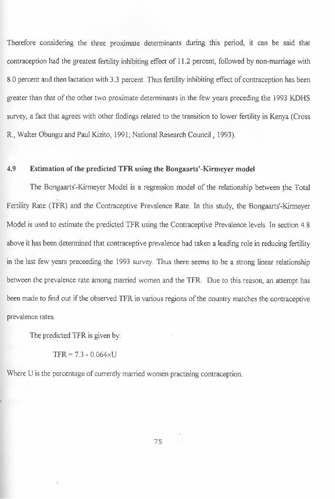
4.9 Estimation of the predicted TFR using the Bongaarts'-Kirmeyer model

The Bongaarts'-Kirmeyer Model is a regression model of the relationship between the Total

Fertility Rate (TFR) and the Contraceptive Prevalence Rate. In this study, the Bongaarts'-Kirmeyer

Model is used to estimate the predicted TFR using the Contraceptive Prevalence levels. In section 4.8

above it has been determined that contraceptive prevalence had taken a leading role in reducing fertility

in the last few years preceeding the 1993 survey. Thus there seems to be a strong linear relationship

between the prevalence rate among married women and the TFR. Due to this reason, an attempt has

been made to find out if the observed TFR in various regions of the country matches the contraceptive

prevalence rates.

The predicted TFR is given by:

TFR = 7.3 - 0.064xU

Where U is the percentage of currently married women practising contraception.

75

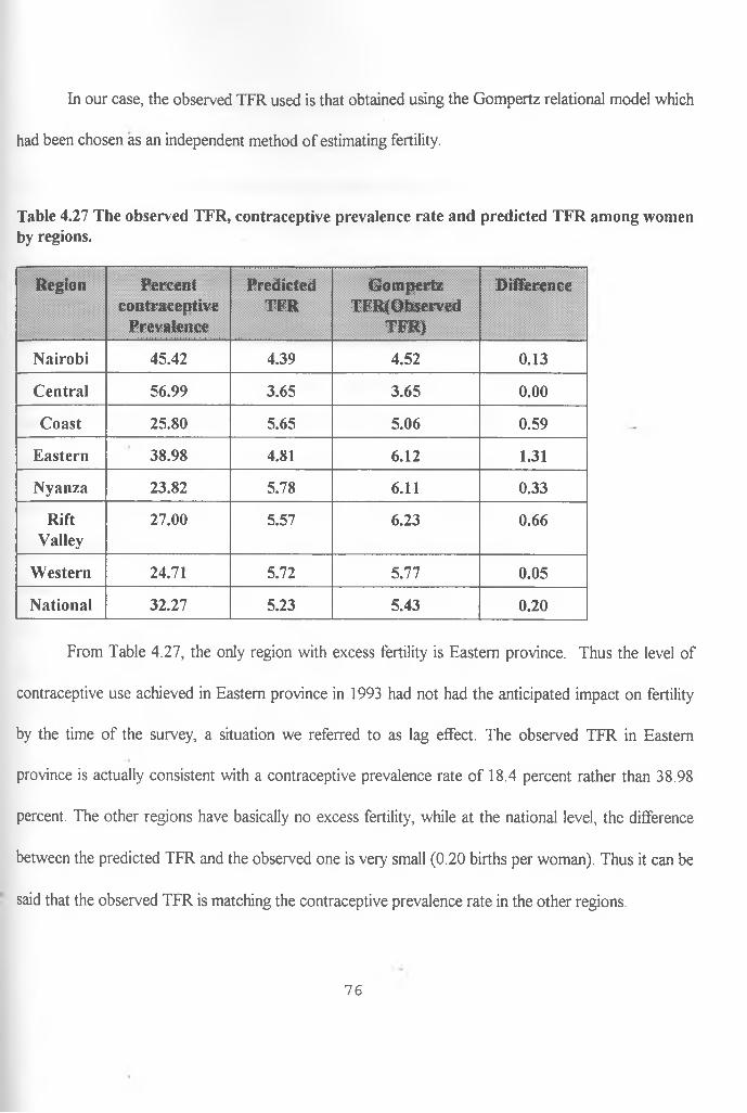
In our case, the observed TFR used is that obtained using the Gompertz relational model which

had been chosen as an independent method of estimating fertility.

Table 4.27 The observed TFR, contraceptive prevalence rate and predicted TFR among women by regions.

Region Percentcontraceptive

Prevalence

PredictedTFR

GompertzTFR(Observed

T i ? m i J f lv J

Difference

Nairobi 45.42 4.39 4.52 0.13

Central 56.99 3.65 3.65 0.00

Coast 25.80 5.65 5.06 0.59

Eastern 38.98 4.81 6.12 1.31

Nyanza 23.82 5.78 6.11 0.33

RiftValley

27.00 5.57 6.23 0.66

Western 24.71 5.72 5.77 0.05

National 32.27 5.23 5.43 0.20

From Table 4.27, the only region with excess fertility is Eastern province. Thus the level of

contraceptive use achieved in Eastern province in 1993 had not had the anticipated impact on fertility

by the time of the survey, a situation we referred to as lag effect. The observed TFR in Eastern

province is actually consistent with a contraceptive prevalence rate of 18.4 percent rather than 38.98

percent. The other regions have basically no excess fertility, while at the national level, the difference

between the predicted TFR and the observed one is very small (0.20 births per woman). Thus it can be

said that the observed TFR is matching the contraceptive prevalence rate in the other regions.

76

From the above findings, it can therefore be said that by setting a given contraceptive

prevalence level, the desired Total Fertility Rate (TFR) can be obtained. The regions with high fertility

in Kenya are the same regions with very low levels of contraceptive prevalence rates. Therefore by

raising the levels of contraceptive prevalence, the TFR in these regions can be reduced to a desired

level.

4.10 Projecting fertility and future demand for contraceptives.

In section 4.9, it has successfully been shown that the observed fertility does actually match the

percentage levels of contraceptive prevalence. This implies that the effect of the other two proximate

determinants estimated in this study is not expected to bring about large effects on TFR in the various

regions of the country. Therefore contraceptive prevalence can be assumed to be the factor which is

going to determine the way the TFR goes in the future. Using this fact and by setting the desired

future levels of fertility, then the corresponding levels of contraceptive prevalence can be estimated and

vice versa. Thus the demand for future contraceptives can be projected as well as the future fertility if

the contraceptive prevalence level is known. The table below gives the projected total fertility rates

obtained from the last population census of 1989 in Kenya.

77

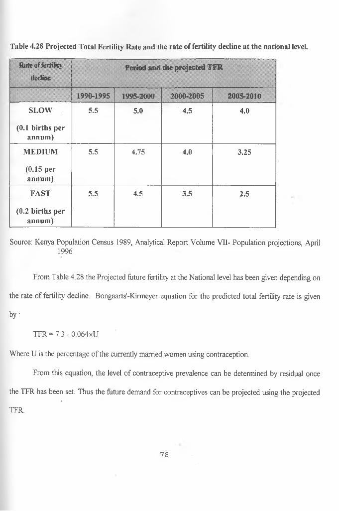
Table 4.28 Projected Total Fertility Rate and the rate of fertility decline at the national level.

Rate of fertility

declinePeriod and the projected TFR

1990-1995 1995-2000 2000-2005 2005-2010

SLOW . 5.5 5.0 4.5 4.0

(0.1 births per annum)

MEDIUM 5.5 4.75 4.0 3.25

(0.15 per annum)

FAST 5.5 4.5 3.5 2.5

(0.2 births per annum)

Source: Kenya Population Census 1989, Analytical Report Volume VII- Population projections, April 1996

From Table 4.28 the Projected future fertility at the National level has been given depending on

the rate of fertility decline. Bongaarts'-Kirmeyer equation for the predicted total fertility rate is given

by:

TFR = 7.3 - 0.064xU

Where U is the percentage of the currently married women using contraception.

From this equation, the level of contraceptive prevalence can be determined by residual once

the TFR has been set. Thus the future demand for contraceptives can be projected using the projected

TFR.

78

Now if we choose a rate of fertility decline of 0.15 births per annum, then for the four periods

1990-1995, 1995-2000, 2000-2005 and 2005-2010, the corresponding projected fertility rates from the

table above are 5.5, 4.75, 4.0 and 3.25 respectively.

But TFR = 7.3-0.064xU. Putting TFR = 5.5, then the predicted contraceptive prevalence rate is

estimated to be

U = (5 .5-7 .3)/-0 .064 = 28.12%

for the period 1990 to 1995.

For the other three periods, the desired contraceptive prevalence rate U is 39.84 percent, 51.56

percent, and 63.28 percent. Hence by choosing any desired rate of fertility decline and the projected

TFR at various periods, the demand for future contraceptives can be estimated.

79

CHAPTER FIVE:

SUMMARY, CONCLUSION AND RECOMMENDATIONS

5.1 Introduction:

The main aim of this study was to determine the fertility level and differentials by

various subgroups in Kenya and to explain these differentials using the proximate

determinants of fertility. The study also sought to find out the contribution of each of the

intermediate fertility variables in inhibiting fertility. The data used in the study was the 1993

Kenya Demographic and Health Survey. The three main proximate determinants estimated in

this study are the index of postpartum infecundability, Q, the index of non-marriage, Cm,

and the index of contraception, Cc. The study also sought to use the contraceptive

prevalence rate to estimate the predicted total fertility rate, TFR, and then compare it with

the observed fertility to determine any regions of excess fertility. An attempt has also been

made to project fertility and demand for future contraceptives.

The data used in the study was drawn from the Kenya demographic and health

survey 1993. This was the second DHS to be carried out in Kenya, the first having been

carried out in 1989. In the survey 7540 women aged between 15-49 years were

interviewed. The survey was designed to provide information on levels and trends of

fertility, infant and child health, and knowledge of AIDS. This survey targeted the same

areas covered in 1989 in order to maintain comparability with the previous survey.

Three models were used in data analyses. The Bongaarts (1978) model was used to

80

estimate the total fertility which was compared to that obtained using the Gompertz

relational model, chosen as an independent method of estimating fertility. Lastly, the

Bongaarts-Kirmeyer regression equation was used to predict TFR and also to project future

demand for contraceptives.

5.2 Summary of the findings.

In section 4.3, the three main proximate determinants of fertility have been estimated

using the Bongaarts (1978) model. This was followed by estimating the total fertility rates,

TFR, using the Bongaarts model and finally using the Gompertz relational model by the

regions, education levels and place of residence. A comparison of the TFR's from the two

models was then done thus achieving the first, second and third objectives of the study.

From the table 4.9, it was shown that the value of the three intermediate fertility variables vary

by the regions, thereby giving rise to different levels of fertility. The values of the indices by the other

subgroups of residence and education also vary widely bringing about differences in fertility among

women in these subgroups. It can be said therefore that the differences in levels of fertility are to be

attributed to the Combined effect of these proximate determinants.

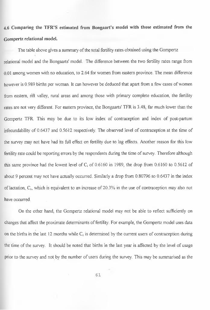
Table 4.14 also gives the fertility rates obtained from the Bongaarts’ model and the Gompertz

relational model. The difference between these fertility rates range from 0.01 to 2.64 births per woman.

These differences are highest among women in Eastern province, those with primary complete

education and those from the rural areas. The lowest differences are found among women in urban

areas and those with no education. The differences in the other categories are quite small, which may

81

be attributed to the usefulness of the proximate determinants in estimating fertility. These large

variations were attributed to various factors that include the following;

(a) Errors in the intermediate fertility variable estimates;

(b) The total fecundity average of 15.3 used for all subgroups that may not hold for all the subgroups;

(c) Assumption that the effect of induced abortion is negligible which is not the case since it has been

found to have significant effect on fertility in many developing countries;

Generally, the fertility rates obtained from the Gompertz relational model are higher than those

obtained from the Bongaarts’ model..

As shown in table 4.9, lactation has the greatest fertility inhibiting effect followed- by non­

marriage while contraception had the least effect. Lactation was found to have the greatest fertility

inhibiting effect in five regions namely Eastern, Rift valley, Western, Nyanza and Coast. However it

had the least effect in Nairobi and Central. Non-marriage had the second greatest fertility inhibiting

effect in all the regions, while contraception was the least fertility inhibiting variable except for Central

and Nairobi where it was the leading fertility inhibiting variable.

The fertility inhibiting effect of lactation decreased with the increase in the level of education.

Thus the index of lactation was lowest among women with no education and highest among those with

secondary and higher level of education. The index of non-marriage decreased with the increase in

education, and so did the index of contraception. Thus the fertility inhibiting effect of these two

variables increased with the increase in the level of education. The inhibiting effect of lactation was

highest among women residing in the rural areas, while that of non-marriage and contraception was

highest among those with the highest level of education. The index of non-marriage was lowest among

82

women with secondary and higher level of education, that of lactation among those in Eastern

province, while that of contraception was lowest among the women in Central province.

From table 4.26, it was noted that there has been an increase in the fertility reducing effect of

all the three intermediate fertility variables during the period 1989 to 1993. At the national level,

lactation has a percent improvement of 3.3, non-marriage 8.0 percent and contraception 11.2 percent.

We can therefore say that during this period, contraception and non-marriage mainly contributed in

achieving the declines in fertility, with lactation playing an almost constant role. This finding is actually

very similar to other findings like that of Cross, Obungu and Kizito(1991) that contraception has

recently been the main cause of fertility decline in many developing countries.

In section 4.9, the only region that was found to have excess fertility was Eastern province

which had a difference of more than one birth between the predicted and the observed fertility. The

other regions had very small differences between the predicted and the observed fertility of less than

one birth. We can therefore say that the observed fertility matches the predicted fertility within the

regions which further suggests that the contraceptive prevalence rate of a certain region does determine

the fertility in that region.

In section 4.10, the future fertility was projected using fertility decline rates on a given

population. Since fertility is expected to match the contraceptive prevalence rates then this rate was

also determined by residue method. Thus the demand for future contraceptives may be estimated in this

manner.

83

5.3 CONCLUSIONS:

The three main proximate determinants of fertility have been estimated in this study and the

resulting total fertility rates obtained using the Bongaarts’ model for all the subgroups considered in

this study. At the national level, the TFR obtained was 4.35, which means an average of about four

births per woman compared to about six births in 1989. This suggests a decline in fertility during the

period 1989 to 1993. At the regional level, Central had the lowest fertility rate of 2.83 compared to 4.5

ofNairobi in 1989. Nyanza had the highest fertility of 5.36 while western had 8.10 as the highest in

1989. From these figures, it can be concluded that there has been a decline in fertility during this

period. We also note that Central took over from Nairobi as the region with the lowest fertility while

Nyanza took over from Western during this period. We can finally conclude that there was a drop in

fertility of between one birth and three births across the regions.

Women in the urban areas had a fertility rate of 3.31, while their counterparts in the rural areas

had a fertility rate of 4.33. In 1989, these rates were 4.99 and 6.66 respectively indicating a drop in

fertility of more than one birth for women in the urban areas and more than two births for those in the

rural areas. There were also very striking differences in fertility for women with different levels of

education. Women with no education had a fertility rate of 5.72 while those with secondary and higher

level of education had a fertility rate of 2.75 births per woman. The corresponding figures were 7.23

and 4.95 respectively in 1989. We therefore conclude that there was also a decline in fertility among

these two subgroups during this period.

Among the three proximate determinants of fertility estimated in this study, we can conclude

that postpartum infecundability was the most important fertility inhibiting variable at the national level

84

and among all the sub-groups except in Nairobi and Central regions, and in the urban areas as well as

among women with secondary and higher level of education. Non-marriage was the second most

important variable at the national level and among all the sub-groups except in the urban areas where it

took the leading role in reducing fertility. Contraception was the most important fertility inhibiting

variable in Nairobi and Central regions, among the women with secondary and higher level of

education and the least important at the national level and the other sub-groups.

There was a general increase in the fertility reduction effect of all the three proximate

determinants during the period prior to the 1993 survey at the national level and across the regions

from the previous section. We can conclude that contraception and non-marriage mainly contributed

towards achieving the declines in fertility between the period 1989 to 1993.

The prediction of fertility using contraceptive prevalence rate indicated that Eastern province

was the only region with excess fertility of more than one birth. The other regions did not have excess

fertility. We can therefore conclude that observed fertility matches with the contraceptive prevalence

rates in these regions. We can also conclude that using this fact, projections for future demand on

contraceptives can be made for any region once the desired future fertility has been determined.

85

<

From the findings of this study, the following recommendations can be drawn;

(i) The women with low fertility are those in Nairobi, Central, urban areas and those with secondary

and higher level of education. This is largely due to effective use o f contraceptives and also non­

marriage. We therefore recommend that the use of effective contraceptives be made available in the

other subgroups with high fertility like Western, Nyanza and Rift valley.

(ii) Since reducing fertility in most populations is an effort towards improving the standards of living in

that population, we recommend that family planning programmes aimed at increasing the use of

effective contraception be intensified throughout the country with emphasis in Nyanza, Western, Rift-

valley and Eastern.

(iii) This study has also shown that there is a positive relationship between the level of education and

use of contraceptives. This in turn has the ultimate result of lowering fertility. We therefore recommend

that the government provide universal education for all and especially for the girls even if it is for free.

(iv) Non-marriage seems to be increasing among women with secondary and higher level of education

and those residing in the urban areas. We recommend that the important role played by marriage in our

society should be re-enforced to the youth in schools and in churches by the respective leaders. At the

same time the importance of breastfeeding in reducing fertility should be brought to the light of the

many youths that do not otherwise know of this fact.

5.4 POLICY RECOMMENDATIONS:

86

5.7 RECOMMENDATIONS FOR FURTHER RESEARCH:

From this study, the following suggestions for further research have been made;

(i) It has been pointed out in this study that induced abortion is increasing in many developing

countries. We suggest that studies be done that includes the effect of induced abortion in reducing

fertility.

(ii) Eastern province was found to be the region with excess fertility. A study to find out the causes of

the excess fertility in this region is useful.

(iii) Population projection studies to be done at regional and district levels so as to enable other

projections to be made like that of future contraceptives.

87

BIBLIOGRAPHY

Anker R. and Knowles J.C. 1980. Human fertility in Kenya, World Employment Programme research

draft: ILO.

Bongaarts, I , and R.G Potter. 1983. An analysis of the proximate determinants in Behaviour, Biology

and Fertility behaviour, studies in Population.

Bongaarts, J., and C. Tietze. 1977. The efficiency o f ' Menstrual regulation as a method fertility

control, centre for Policy studies Working papers. The Population Council, New York

Bongaarts, J., and S. Kirmeyer. 1982. Estimating the impact of contraceptive prevalence on fertility:

Aggregate and age-specific versions of a model in Hermatin A. I. and E. Barbara (Ed.). The

role of Surveys in the analysis of Family Planning Programmes.

Bongaarts, J. 1978. A framework for analysing the proximate determinants of fertility in

Population and Development review 4. No. 1: Pig. 105-132.

..........1984. Implications of future fertility trends for contraceptive practice in Population

and Development Review 10, No. 2: Pg. 341-352.

.......... 1979. The fertility impacts of Traditional and changing child-spacing practices in Tropical

Africa, Working Paper No. 42, Centre for Policy Studies. Population Council, New York.

...........1980. The fertility-inhibiting effects of the intermediate fertility variables in centre for Policy

Studies, Working Papers, No. 57. The Population Council, New York.

88

V

........... 1987. The proximate determinants of exceptionally high fertility in Population and Develop

Review 13 No. 1

........... 1982. The Fertility-Inhibiting Effects of the intermediate fertility variables in Studies in Family

Planning, Vol. 13. No. 6/7.

1983. Fertility, Biology and Behaviour: An analysis of the proximate determinants. New York

Academic Press.

Brass W. 1974. Perspectives in Population Prediction: Illustrated by Statistics of England and Wales.

J.R.S.S. Vol. A, No.137. .

Brass W. 1981. The use of Gompertz relational model to Estimate Fertility. The IUSSP conference,

Manila.

Booth H. 1977. The estimation of fertility from incomplete cohort data by means of the transformed

Gompertz model. PhD. Thesis, University of London.

Caldwell, J. C., and P. Caldwell. 1977. The role of marital sexual Abstinence in Determining Fertility: a

study of Yoruba in Nigeria. Population Studies Vol. 31

Cleland J., and Hobcraft J. 1985. Reoroductive change in developing countries: Insights from the

World Fertility Survey: Oxford University Press. New York.

Cross, R. A., W. Obungu and P. Kizito. 1991. Evidence of a transition to lower fertility in Kenya in

International Family Planning Perspectives, Vol. 17, No. 1: Pg. 4-7.

89

Curtis, S. L., and I. Diamond. 1995. When Fertility seems too high for contraceptive prevalence: An

analysis of NorthEast Brazil in International Family Planning Perspectives, Vol. 21. No. 2: Pg.

58-63.

Davis, K., and X. Blake. 1956. Social structure and Fertility. An Analytic Framework. Economic

Development and Cultural Change Vol. 4, No. 4: Pg. 211-235.

Ferry, B., and H. J. Page. 1984. The Proximate determinants of Fertility and their effect on Fertility

Patterns: an illustrative Analysis Applied in Kenya, World Fertility Survey, Scientific Report

No. 71. Voorburg, Netherlands: International Statistical Institute.

Frank 0 . 1980. Infertility in Sub-Saharan Africa: The population council. New York.

Gaisie, S. K. 1984. The proximate determinants of fertility in Ghana Scientific Reports No. 53.

Voorburg, Netherlands: International Statistical Institute.

Gaslonde, S. 1982. The impact of some intermediate variables on Fertility: Evidence from the

Venezuela National Fertility Survey, 1977.

Goldscheider C. and Mosher W.D. 1988. Religious affiliations and contraceptive usage: Changing

American patterns, 1955-82 in Studies in Family Planning, Vol. 19, Nol.

Heidi B.J. and Kenneth H.H. 1996. Induced abortion in the developing world: Indirect estimates in

International family Planning Perspectives, Vol. 22, No.3.

Hobcraft J. and Little R.J.A. 1984. Fertility exposure analysis: A new method for assessing the

contribution of proximate determinants to fertility differentials: Population studies, Vol.38,

No.l.

90

Kalule-Sabiti. 1984. Proximate determinants of Fertility Applied to Data from the Kenya Fertility

Survey (1977/78); Journal of Biological Science, 16 WFS, International Statistical Institute,

London.

Komba A.S. and Kamuzora C.L. 1988. Fertility reduction due to non-marriage and lactation: A case

study of Kibaha district, Tanzania, in Africa Population conference, Vol. 1, Dakar, IUSSP,

UAPS. .

Mosley W.H., Osteria T. and Huffman S.L. 1977. Interactions of contraception and breastfeeding in

developing countries: Reprint from the journal of bio-social science, Suppl. 4.

Mosley W.H. and Werner L.H. 1980. Some determinants of marital fertility in Kenya: a birth interval

analysis from the 1978 Kenya Fertility Survey: PSRI. University of Nairobi.

Mosley W.H., Werner L.H. and Becker S. 1982. The dynamics of birth spacing and marital fertility in

Kenya: Voorburg, Netherlands: Internal Statistical Institute.

Mwobobia, I. K. 1982. Fertility differentials in Kenya: Across regional study. MA thesis, Population

Studies and Research Institute, University of Nairobi.

National Research Council. 1993. Population Dynamics o f Kenya: National Academy Press. Washington D.C.

Nortman, D.L. 1980. Empirical patterns o f Contraceptive use: A review in the nature and sourcesof data and recent findings: Population council. New York.

Page, H.J., Lesthaeghe, R.J. and Shah, I.H. 1982. Illustrative Analysis: Breasfeeding in Pakistan. World Fertility Survey, Scientific report No.37, Voorburg, Netherlands:Internal Statistical Institute.

91

Ocholla-Ayayo and Z. Muganzi. 1986. Field report in Nyanza and Western Provinces ongoing research

on Marital Patterns of fertility determinants with differential effects among ethnic groups in

Kenya.

Omagwa. 1986. The influence of social-economic and demographic factors on fertility levels in

Nairobi. MSc. thesis Population Studies and Research Institute, (PSRI), University of Nairobi.

Omurundo, J.K. 1989. Infant / Child Mortality and Fertility rates in Western Province o f Kenya. M.sc Thesis, PSRI. University of Nairobi.

Osiemo, J. A. O. 1986. Estimation of fertility levels and differentials in Kenya: An application of Coale-

Trussell and Gompertz Relational Models,. MSc. thesis, PSRI, University of Nairobi. -

Potter, R.G. 1963. Birth intervals: Structure and change. Population studies Vol. 17.

Potter, R.G., Kobrin, F.E., and Langsten, R.L. 1979. Comparison of three acceptance Strategies: A progress report. Honolulu Hawaii: East-west Center.

Rodriguez, G. and Cleland, J. 1987. The effects of parental education, marital fertility in developing countries: The population council. New York.

Sheps, C.M. 1964. Applications of probability models to the study o f patterns of Human Reproduction in Public Health and Population change. IUSSP.

Singh, S., Casterline, B. and Cleland, J.G. 1985. The proximate determinants of Fertility: Sub­national variations: Population studies, Vol. 38, No. 1

Tietze, C. 1964. History and Statistical evaluation of Intra-uterine Contraceptive Device in Public Health and Population change, University o f Pittsburg Press.

Wamalwa, M. W. 1991. Bongaarts' Model of proximate determinants of fertility applied to the Kenya

Demographic and Health Survey 1989 Data, MSc. thesis, PSRI, University of Nairobi.

92

Zaba. 1981. Use of Relational Gompertz model in Analysing fertility data collected in Retrospective Surveys. CPS working Paper 81-2. London School o f Hygiene.

93

APPENDIX A: COMPUTATION OF THE TOTAL FERTILITY RATES USING THEBONGAARTS’ MODEL

NAIROBI

1. computation of index of post-partum infecundability, C j

age group

. • .::x:xx;:;xxx;:;x:::x;x:xix:::::x::::

xx:^•IxtXv^vXvXtXvX^^XX^vX1

children born 0-35 months prior to

' survey• • • . . .

children“ a m Z T y "

'1 9 1 5

2 53-

28

3 39-

18

4 19-

9

5 6-

4

6 3-

1

7 1-

1

Total 130 1 66

C = 20/18.S4iwhere i= 1.753eaiwWM01™

B = mean duration of breastfeeding.

B = P/I

I = births 0-35 months +l/2(aged 36 months)/36

=130+l/2(l)/36 =3.25

B = 66/3.25 =18.21

94

i = 11.97

hence Q = 20/18.5

2. Computation of index of non-marriage, Cm

age group

"■

femalepopulation

(FFOP)

marriedwomen

proportionmarried,

m(a)• :

births inthe last 12■■ • ...

; months• •(BL12)

age specific fertility

mtes. fWI l l i l l l l l ! !

5= Is

||

f|

1 58 14 0.2414 7 0.1207 0.2090

2 126 61 0.4841 17 0.1349 0.2787

3 78 52 0.6667 13 0.1667 0.2500

4 46 29 0.6304 6 0.1304 0.2069

5 25 17 0.6800 2 0.0800 0.1176

6 20 13 0.6500 - 0.0000 0.0000

7 14 10 0.7143 1 0.0714 0.1000

Total 367 196 4.0669 46 0.7041 1.1622

Cm= sum f(a)/sum g(a) = 7041/1.1622 =0.6058

95

3. Computation of the index of contraception, Cc

method;:

Pill 40 0.2041 0.90000 0.1837

IUD 19 0.0969 0.9500 0.0921

Female v sterilisation

4 0.0205 1.0000 0.0205

Others 26 0.1327 0.7000 0.0929

Total 89 0.4542 0.3892

Cc=l-1.08(U)(E)

E = sum U(m)e(m)/sum U(m) =0.3892/0.4542 = 0.8569)

Cc= 1-1.08(0.4542)0.8569 = 0.5797

96

CENTRAL

1. Computation of the index of infecundability, Q

111!!!__ ..................................... r r z , , ! ..... ............ ..........................children bom 0-36 children exactly 36 no. O f women

months pnor to months currently« » » n /A V ! % 1^uivey uF?ifeueeuiug

1 30-

22

2 120 2 61

3 105 3 53

4 80-

43

5 29 1 17

6 16 2 7

7 3-

1

Total 383 8 204

C;=20/18.5+i where i=1.753e0 1396B'<)001872B2

B= P/I =(383+l/2(8))/36 =204/10.68 =19.11

1=12.75

Q = 20/18.5+12.75 =0.6400

2. Computation of the index of non-marriage, Cm

97

219

168

168

98

128

135

0.4475

0.7619

0.8036

30

32

32

0.1370

0.1905

0.1905

0.2296

0.3061

0.2500

0.2370

92 77 0.8370 11 0.1196 0.1428

110 84 0.7636 0.0273 0.0357

80 65 0.8125

Total 1075 600 125 0.7363 1.2012

Cm= sum f(a)/sum g(a)

= 0.7363/1.2012=0.6130

3. Computation of the index of contraception, Cc

me! hod no. of married women using

method

U(m) e(m)’

s •

U(m)e<m)■ .v . :« •> : .• • • :

v $ \ :: ' •: . ::? ••• . :.• •• •*Pill 108 0.1800 0.9000 0.1695

IUD 63 0.1050 0.9500 0.0998

Sterilisation 53 0.0883 1.0000 0.0883

Others 113 0.1883 0.7000 0.1318

Total 337 0.5699 0.4894

Cc= 1 -1.08(U)(E)

E = 0.8588

98

Cc =0.4714

COAST

1. Computation of the index of infecundability, Q

age group

i i l i i l i l l i l

children bom 0- 35 months pnor

to the survey

children exactly 36 months

• • -.V. •. •

no of women ‘ .

breastfeeding

1 42-

27

2 138—

74

3 110 4 63

4 84 12 46

5 58—

40

6 9 1 8

7 7—

5

Total 448 17 263

Q = 20/18.5+1

i = 14.17

Ci= 20/18.5+14.17 = 0.6122

2. Computation of the index of non-marriage, Cm

99

agegroup

fpop marriedfpop

3?s BL12: ? %

g(a)

1 278 52 0.1871 21 0.0755 0.3112

2 222 135 0.6081 56 0.2523 0.4149

3 177 142 0.8023 40 0.2260 0.2817

4 164 133 0.8110 29 0.1768 0.2180

5 131 103 0.7863 22 0.1679 0.2135

6 64 44 0.6875 5 0.0781 0.1136

7 55 42 0.7636 3 0.0545 0.0714

Total 1091 651 174 1.0311 1.6243

Cm = I f(a)/I g(a)

= 1.0311/1.6243 = 0.6348

3. Computation of the index of contraception, Cc

method married women using method !i

§ i

____ e(m)

iii i i l l i i i i i i i i i

U(m)e(m)

.

Pill 52 0.0799 0.9000 0.0719

IUD 20 0.0307 0.9500 0.0292

Sterilisation 23 0.0353 1.0000 0.0353

Others 73 0.1121 0.7000 0.0785

Total 168 0.2580 0.2149

Cc= 1-1.08(U)(E)

E = 0.8328 Cc = 0.7680

100

EASTERN

1. Computation of the index of infecundability, Q

age

. ?.

children 0-35 months prior to the survey

children exactly 36

months

no. of women currently

breastfeeding1

1 41—

29

2 147 2 110

3 109 3 72

4 102 6 67

5 54 3 33

6 33 4 23

7 10-

5

Total 496 18 339

Ci =20/18.5+1

i = 17.14

Ci = 20/18.5+17.14 = 0.5612

101

2. Computation of the index of non-marriage, Cm

^ ,

1 221' 23 0.1041 23 0.1041 0.4145

2 214 114 0.5327 63 0.2944 0.5527

3 162 133 0.8210 43 0.2654 0.3233

4 160 140 0.8750 37 0.2313 0.2643

5 105 88 0.8381 19 0.1810 0.2160

6 125 101 0.8080 14 0.1120 0.1386

7 57 50 0.8772 3 0.0526 0.0600

Total 1044 649 202 1.2408 1.9694

Cm = sum f(a)/sum g(a) =1.2408/1.9694 = 0.6300

3. Computation of the index of contraception, Cc

method married women using

method

U(m)

■

U(m)e<m)

Pill 85 0.1310 0.9000 0.1179

IUD 38 0.0586 0.9500 0.0556

Sterilisation 35 0.0539 1.0000 0.0539

Others 95 0.1464 0.7000 0.1025

Total 253 0.3898 0.3299

Cc=l-1.08(U)(E)

E = 0.8462 Cc =0.6437

102

NYANZA

1. Computation of the index of infecundability, Q

age group .......: ̂ ^ poor to survey | ,„„„Ihs | breastfeeding

1 72 — 46

2 193 5

3 175 7 107

4 123 3 99

5 47 3 66

6 26 2 24

7 8 1 16

Total 644 21 360

20/18.5+i; i = 13.35 =>Q = 20/18.5+13.35 = 0.6279

2. Computation of the index of non-marriage, Cm

age group fpop married fpop m(a) BL12 f(a) 8(a)

1 318 64 0.2013 36 0.1132 0.3132

2 258 170 0.6589 71 0.2752 0.4177

3 181 157 0.8674 69 0.3812 0.4395

4 199 175 0.8794 42 0.2111 0.2401

5 110 84 0.7636 16 0.1455 0.1905

6 119 95 0.7983 11 0.0924 0.1157

7 79 57 0.7215 2 0.0253 0.0351

Total 1264 802 247•>

1.2439 1.7518

103

Cm = sum f(a)/sum g(a) = 1.2439/1.7518

= 0.7100

3.Computation of the index of contraception, Cc

method marriedusingmethod

•e(m)

: ■ :Pill 32 0.0399 0.9000 0.0359

IUD 9 0.0112 0.9500 0.0106

Sterilisation 55 0.0686 1.0000 0.0686

Others 95 0.1185 0.7000 0.0830

Total 191 0.2382 0.1981

Cc= 1-1.08 (U)(E) ; E = 0.8317 => Cc = 0.7861

RIFT-VALLEY

1. Computation of the index of infecundability, Q

age group

• • :

children 0-35 months children exactly 36 months

| f ? women currently breastfeeding

1 71 1 49

2 266 9 152

3 234 13 139

4 169 7 99

5 84 3 55

6 43 4 32

7 16 — 10

Total 883 37■s

536

104

Ci = 20/18.5+1; i =14.76 => Ci = 20/18.5+14.76 = 0.6013

2. Computation of the index of non-marriage, Cm

g g p pop■Don

m(a)5

i i i i i l l i iB U Z |Ya\1(a) m: •: \ V • .

l i f t ! ! ! ! ! ! ! !

1 423 51 0.1206 35 0.0827 0.3440

2 373 218 0.5845 100 0.2681 0.4587

3 305 256 0.8393 88 0.2885 0.3437

4 250 207 0.8280 68 0.2720 0.3285

5 162 136 0.8395 33 0.2037 0.2426

6 142 125 0.8803 15 0.1056 0.1200

7 99 81 0.8182 8 0.0808 0.0988

Total 1794 1074 347 1.3014 1.9363

Cm =f(a)/g(a) =1.3014/1.9363 = 0.6721

3. Computation of the index of contraception, Cc

method women using method

U(m) e(m) TJ(m)e(m)

Pill 41 0.0382 0.9000 0.0344

IIJD 19 0.0177 0.9500 0.0168

Sterilisation 66 0.0615 1.0000 0.0615

Others 164 0.1527 0.7000 0.1069

Total 290 0.2700 0.2195

Cc=l-1.08(U)(E)

E = 0.8129 => Cc = 0.7629

105

WESTERN1. Computation of the index of infecundability,Cj

age group children 0-35 mouths children exactly 36 months

women currently breastfeeding

1 47 — 33

2 139 2 80

3 119 1 64

4 104 3 67

5 68 2 42

6 28 2 19

7 7 — 1

Total 512 10 306

Q = 20/18.5+1; i = 14.67 => Ci = 0.6030

2. Computation of the index of non-mareiage, cm

age group fpop married fpop m(a) JBL12 f(a) g(a)

1 252 44 0.1746 28 0.1111 0.3100

2 193 121 0.6269 50 0.2591 0.4133

3 128 110 0.8594 34 0.2656 0.3091

4 125 113 0.9040 32 0.2560 0.2832

5 118 106 0.8983 18 0.1525 0.1698

6 73 68 0.9315 7 0.0959 0.1030

7 56 49 0.8750 1 0.0179 0.0205

Total 945 611 170 1.1581 1.6089

106

Cm = f(a)/g(a)= 1.1581/1.6089 =0.7198

3. Computation of the index of contraception, Cc

method married using methodo \ N . £ 'o '•

xvxv x v x -x *x v x -x x ” x x * x * x ;x:x::::;x#^^mu U(m)e(m)

Pill 36 0.0589 0.9000 0.0530

IUD 12 0.0196 0.9500 0.0187

Sterilisation 25 0.0409 1.0000 0.0409

Others 78 0.1277 0.7000 0.0894

Total 151 0.2471 0.2020

Cc= 1-1.08 (U )(E);E = 0.8172

Cc = 0.7819

URBAN

1. Computation of the index of lactation, Cj

C j = 20/18.5+i

i = 12.37

Q = 0.6479.

2. Computation of the index of non-marriage, Cm

age group•

fpop marriedfpop

B U 2m

*:*:::»:::*:*:“:::*:*:::*$*:*A*:*:*:*:*:*:*&*:*:*:.:C::'

* » )

1 246 32 0.1301 15 0.0610 0.2500

2 319 156 0.4890 52 0.1630 0.3333

3 230 163 0.7087 36 0.1565 0.2208

4 176 124 0.7045 24 0.1364 0.1936

5 98 65 0.6632 7 0.0714 0.1077

107

V

6 57 39 0.6842 3 0.0526 0.0769

7 35 28 0.8000 1 0.0286 0.0358

Total 1161 607 138 0.6695 1.2181

Cm = f(a)/g(a) = 0.6695/1.2181

= 0.5496

3. Computation of the index of contraception, Cc

method married using method

U(m) « .» )

Pill 90 0.1483 0.9000 0.1335

IUD 53 0.0873 0.9500 0.0829

Sterilisation 33 0.0544 1.0000 0.0544

Others 80 0.1318 0.7000 0.0923

Total 256 0.4218 0.3631

Cc = 1-1.08(U)(E)

E = 0.8607

Cc = 0.6079

RURAL

1. Computation of the index of lactation, Q

1 Ci = 20/18.5+i

i = 14.69

108

Ci = 0.5765

2. Computation of index of non-marriage, Cm

age group fpop

l i l i i i i l

.........................■»(*) BL12 r w

1 1542 229 0.1485 152 0.0986 0.3301

2 1286 761 0.5918 335 0.2605 0.4402

3 969 815 0.8411 283 0.2921 0.3472

4 936 808 0.8632 222 0.2372 0.2748

5 645 546 0.8465 114 0.1767 0.2088

6 596 491 0.8238 52 0.0872 0.1059

7 405 326 0.8049 17 0.0420 0.0521

Total 6379 3976 1175 1.1943 1.7591

Cm=f(a)/g(a) =1.1943/1.7591

= 0.6789

3. Computation of the index of contraception, Cc

method married using method U(m) > ■ s r:: U(m)e(in)

Pill 304 0.0765 0.9000 0.0688

IUD 127 0.0319 0.9500 0.0303

Sterilisation 228 0.0573 1.0000 0.0573

Others 564 0.1419 0.7000 0.0993

Total 1223 0.3076 0.2557

' Ce= 1-1.08 (U )(E);E = 0.8313

Cc = 0.7238

109

NO EDUCATION

1. Computation of the index of lactation, Q

Q = 20/18.5+i

i= 16.00

Q = 0.5797

2. Computation of the index of non-marriage, Cm

age group fpop marriedfpop

m(a) BL12; I I J s ) g(a)

1 60 20 0.3333 8 0.1333 0.2298

2 82 62 0.7561 19 0.2317 0.3064

3 142 123 0.8662 43 0.3028 0.3496

4 235 205 0.8723 61 0.2596 0.2976

5 262 204 0.7786 51 0.1947 0.2501

6 269 211 0.7844 24 0.0892 0.1137

7 247 194 0.7854 13 0.0526 0.0670

Total 1297 1019 219 1.2639 1.6142

Cm = f(a)/g(a) =1.2639/1.6142

= 0.7830

110

3. Computation of the index of contraception, Cc

method*

U(m)x xx Vxx -^ xxx fx ;1 •

e(m) 1

Pill 28 0.0275 0.9000

0.0248

IUD 11 0.0108 0.9500

0.0103

Sterilisation 61 0.0599 1.0000

0.0599

Others 100 0.0981 0.7000

0.0687

Total 200 0.1963 0.1636

Cc= 1- 1.08(U)(E);E = 0.8333

Cc = 0.8233

PRIMARY INCOMPLETE

1. Computation of the index of lactation, Q

Ci = 20/18.5+i; i = 14.03

Ci = 0.6148

111

V

2. Computation of the index of non-marriage, Cm

age group fpop married fpop m(a) BL12 m g «

1 1035 167 0.1617 97 0.0937 0.3117

2 663 450 0.6787 187 0.2821 0.4156

3 347 302 0.8703 114 0.3285 0.3775

4 359 306 0.8524 81 0.2256 0.2647

5 237 200 0.8439 38 0.1603 0.1900

6 266 223 0.8383 23 0.0865 0.1031

7 142 113 0.7958 4 0.0282 0.0354

Total 3049 1761 544 1.2049 1.6980

Cm= f(a)/g(a) = 1.2049/1.6980

= 0.7115

3. Computation of the index of contraception, Cc

method marriedusing

method

U(m) e(m) tJ(m)e(m)

Pill 108 0.0613 0.9000 0.0552

IUD 49 0.0278 0.9500 0.0264

Sterilisation 96 0.0545 1.0000 0.0545

Others 225 0.1278 0.7000 0.0895

Total 478 0.2714 0.2255

Cc= 1-1.08(U)(E) ; E = 0.8310

Cc = 0.7564

S'

1 1 2

PRIMARY COMPLETE

1. Computation of the index of lactation, Q

Q = 20/18.5+i

i = 14.50

C; = 0.6061

2. Computation of the index of non-marriage, Cm

fp»» marriedi l l l l l l l i l p * » g(a)

1 315 46 0.1460 36 0.1143 0.3419

2 342 204 0.5965 93 0.2719 0.4558

3 289 235 0.8131 78 0.2699 0.3319

4 234 192 0.8205 52 0.2222 0.2708

5 126 107 0.8492 17 0.1349 0.1589

6 64 57 0.8906 7 0.1094 0.1228

7 30 28 0.9333 — 0.0000 0.0000

Total 1400 869 283 1.1226 1.6821

Cm = f(a)/g(a) =1.1226/1.6821

= 0.6674

e

113

3. Computation of the index of contraception, Cc

m y | f |Pill 104 0.1197 0.9000 0.1077

IUD 30 0.0345 0.9500 0.0328

Sterilisation 50 0.0575 1.0000 0.0575

Others 138 0.1588 0.7000 0.1112

Total 322 0.3705 0.3092

Cc =1-1.08(U)(E); E = 0.8345 => Cc= 0.6661

SECONDARY AND HIGHER

1. Computation of the index of lactation, Ci

C; = 20/18.5+i; i= 13.82 => C;= 0.6188

2. Computation of the index of non-marriage, Cm

age group fpop marriedfpop

m(a) BL12 f(a) g(a)

1 378 28 0.0741 26 0.0688 0.3284

2 518 201 0.3880 88 0.1699 0.4379

3 421 318 0.7553 85 0.2019 0.2673

4 284 229 0.8063 53 0.1866 0.2314

5 118 100 0.8475 15 0.1271 0.1500

6 54 39 0.7222 1 0.0185 0.0256

7 21 19 0.9048 1 0.0476 0.0526

Total 1794 934 269 0.8204 1.4932

Cm= f(a)/g(a) =0.8204/1.4932 = 0.5494

114

3. Computation of the index of contraception, Cc

married using ITt

Pill 147 0.1574 0.9000 0.1416

IUD 84 0.0899 0.9500 0.0854

Sterilisation 63 0.0675 1.0000 0.0675

Others 189 0.2024 0.7000 0.1416

Total 322 0.5172 0.4361

Ce l-1.08(U)(E)

E = 0.8432

Cc = 0.5290

115

*