This article was downloaded by: [Lund University Libraries] On: 19 August 2014, At: 00:23 Publisher: Taylor & Francis Informa Ltd Registered in England and Wales Registered Number: 1072954 Registered office: Mortimer House, 37-41 Mortimer Street, London W1T 3JH, UK Hydrological Sciences Journal Publication details, including instructions for authors and subscription information: http://www.tandfonline.com/loi/thsj20 Soil water content and salinity determination using different dielectric methods in saline gypsiferous soil / Détermination de la teneur en eau et de la salinité de sols salins gypseux à l'aide de différentes méthodes diélectriques FETHI BOUKSILA a , MAGNUS PERSSON b , RONNY BERNDTSSON b & AKISSA BAHRI a a National Institute for Research in Rural Engineering, Waters and Forests , Box 10, 2080, Ariana, Tunisia b Department of Water Resources Engineering , Lund University , Box 118, 221 00, Lund, Sweden E-mail: Published online: 18 Jan 2010. To cite this article: FETHI BOUKSILA , MAGNUS PERSSON , RONNY BERNDTSSON & AKISSA BAHRI (2008) Soil water content and salinity determination using different dielectric methods in saline gypsiferous soil / Détermination de la teneur en eau et de la salinité de sols salins gypseux à l'aide de différentes méthodes diélectriques, Hydrological Sciences Journal, 53:1, 253-265 To link to this article: http://dx.doi.org/10.1623/hysj.53.1.253 PLEASE SCROLL DOWN FOR ARTICLE Taylor & Francis makes every effort to ensure the accuracy of all the information (the “Content”) contained in the publications on our platform. However, Taylor & Francis, our agents, and our licensors make no representations or warranties whatsoever as to the accuracy, completeness, or suitability for any purpose of the Content. Any opinions and views expressed in this publication are the opinions and views of the authors, and are not the views of or endorsed by Taylor & Francis. The accuracy of the Content should not be relied upon and should be independently verified with primary sources of information. Taylor and Francis shall not be liable for any losses, actions, claims, proceedings, demands, costs, expenses, damages, and other liabilities whatsoever or howsoever caused arising directly or indirectly in connection with, in relation to or arising out of the use of the Content. This article may be used for research, teaching, and private study purposes. Any substantial or systematic reproduction, redistribution, reselling, loan, sub-licensing, systematic supply, or distribution in any form to anyone is expressly forbidden. Terms & Conditions of access and use can be found at http:// www.tandfonline.com/page/terms-and-conditions
Transcript
This article was downloaded by: [Lund University Libraries]On: 19 August 2014, At: 00:23Publisher: Taylor & FrancisInforma Ltd Registered in England and Wales Registered Number: 1072954 Registered office: MortimerHouse, 37-41 Mortimer Street, London W1T 3JH, UK
Hydrological Sciences JournalPublication details, including instructions for authors and subscription information:http://www.tandfonline.com/loi/thsj20
Soil water content and salinity determination usingdifferent dielectric methods in saline gypsiferoussoil / Détermination de la teneur en eau et de lasalinité de sols salins gypseux à l'aide de différentesméthodes diélectriquesFETHI BOUKSILA a , MAGNUS PERSSON b , RONNY BERNDTSSON b & AKISSA BAHRI aa National Institute for Research in Rural Engineering, Waters and Forests , Box 10, 2080,Ariana, Tunisiab Department of Water Resources Engineering , Lund University , Box 118, 221 00, Lund,Sweden E-mail:Published online: 18 Jan 2010.
To cite this article: FETHI BOUKSILA , MAGNUS PERSSON , RONNY BERNDTSSON & AKISSA BAHRI (2008) Soil water contentand salinity determination using different dielectric methods in saline gypsiferous soil / Détermination de la teneur eneau et de la salinité de sols salins gypseux à l'aide de différentes méthodes diélectriques, Hydrological Sciences Journal,53:1, 253-265
To link to this article: http://dx.doi.org/10.1623/hysj.53.1.253
PLEASE SCROLL DOWN FOR ARTICLE
Taylor & Francis makes every effort to ensure the accuracy of all the information (the “Content”) containedin the publications on our platform. However, Taylor & Francis, our agents, and our licensors make norepresentations or warranties whatsoever as to the accuracy, completeness, or suitability for any purpose ofthe Content. Any opinions and views expressed in this publication are the opinions and views of the authors,and are not the views of or endorsed by Taylor & Francis. The accuracy of the Content should not be reliedupon and should be independently verified with primary sources of information. Taylor and Francis shallnot be liable for any losses, actions, claims, proceedings, demands, costs, expenses, damages, and otherliabilities whatsoever or howsoever caused arising directly or indirectly in connection with, in relation to orarising out of the use of the Content.
This article may be used for research, teaching, and private study purposes. Any substantial or systematicreproduction, redistribution, reselling, loan, sub-licensing, systematic supply, or distribution in anyform to anyone is expressly forbidden. Terms & Conditions of access and use can be found at http://www.tandfonline.com/page/terms-and-conditions
Soil water content and salinity determination using different dielectric methods in saline gypsiferous soil FETHI BOUKSILA1, MAGNUS PERSSON2, RONNY BERNDTSSON2 & AKISSA BAHRI1
1 National Institute for Research in Rural Engineering, Waters and Forests, Box 10, 2080 Ariana, Tunisia 2 Department of Water Resources Engineering, Lund University, Box 118, 221 00 Lund, Sweden
[email protected] Abstract Measurements of dielectric permittivity and electrical conductivity were taken in a saline gypsiferous soil collected from southern Tunisia. Both time domain reflectometry (TDR) and the new WET sensor based on frequency domain reflectometry (FDR) were used. Seven different moistening solutions were used with electrical conductivities of 0.0053–14 dS m-1. Different models for describing the observed relationships between dielectric permittivity (Ka) and water content (θ), and bulk electrical conductivity (ECa) and pore water electrical conductivity (ECp) were tested and evaluated. The commonly used Ka–θ models by Topp et al. (1980) and Ledieu et al. (1986) cannot be recommended for the WET sensor. With these models, the RMSE and the mean relative error of the predicted θ were about 0.04 m3 m-3 and 19% for TDR and 0.08 m3 m-3 and 54% for WET sensor measurements, respectively. Using the Hilhorst (2000) model for ECp predictions, the RMSE was 1.16 dS m-1 and 4.15 dS m-1 using TDR and the WET sensor, respectively. The WET sensor could give similar accuracy to TDR if calibrated values of the soil parameter were used instead of standard values. Key words soil salinity; gypsiferous soils; time domain reflectometry (TDR); frequency domain reflectometry (FDR)
Détermination de la teneur en eau et de la salinité de sols salins gypseux à l’aide de différentes méthodes diélectriques Résume Des mesures de permittivité diélectrique et de conductivité électrique ont été réalisées sur des sols gypso-salins prélevés dans le sud tunisien. Les deux méthodes de réflectométrie dans le domaine temporel (TDR) et de réflectométrie dans le domaine fréquentiel (FDR) ont été utilisées. Sept solutions d’humectation, de conductivité électrique variant de 0.00053 à 14 dS m-1, ont été appliquées. Différents modèles pour décrire les relations observées entre la permittivité diélectrique (Ka), la teneur en eau (θ), la conductivité électrique apparente (ECa) et la conductivité électrique de la solution des sols (ECp) ont été testés et évalués. Les modèles courants de type Ka–θ de Topp et al. (1980) et de Ledieu et al. (1986) sont déconseillés pour la sonde WET. Avec ces modèles, la racine de l’erreur quadratique moyenne (RMSE) et la moyenne des erreurs résiduelles (MRE) de θ sont respectivement d’environ 0.04 m3 m-3 et 19% pour la TDR et de 0.08 m3 m-3 et 54% pour les mesures avec la sonde WET. En utilisant le modèle de Hilhorst (2000), la RMSE de la ECp estt de 1.16 dS m-1 avec les mesures TDR et atteint 4.15 dS m-1 avec les mesures de la sonde WET. La sonde WET peut donner une précision similaire à celle de la TDR dans le cas d’une utilisation de valeurs calées du paramètre sol à la place des valeurs standard. Mots clefs salinité des sols; sol gypseux; réflectométrie dans le domaine temporel (TDR); réflectométrie dans le domaine fréquentiel (FDR) INTRODUCTION
According to FAO (1990), gypsiferous soils are widespread in arid areas with an annual precipitation less than about 400 mm and where sources of calcium sulfate exist. Globally they occupy about 85 million ha, 54.6% in Africa, 44.9% in Asia, 0.4% in Europe, and 0.1% in North America. In Tunisia, gypsiferous soils cover 9.3% of the country. The physical, chemical, and thermal properties of gypsiferous soils are different to those of other mineral soils (Pouget, 1965; 1968; Vieillefon, 1979; FAO, 1990; Escudero et al., 2000). Gypsum is a soluble salt: hydrous calcium sulfate CaSO4 2H2O, containing 20.9% of water. Gypsum can be transformed into anhydrite (CaSO4) upon heating. At 70–90°C the gypsum is transformed to the semi-hydrate bassanite (CaSO4,0,5H2O) and to anhydrite (CaSO4) at 105°C in a dry oven (Pouget, 1965) or at about 200°C in a ventilated oven (Vieillefon, 1979). The solubility of the gypsum is 2.6 g/L of pure water at 25°C. According to Vieillefon (1979), its solubility is influenced by several parameters, e.g. the salinity; in solutions with calcium bicarbonate and sodium sulfate ions, the solubility of gypsum decreases while others ions increase
it. In a solution containing about 120–130 g/L of NaCl or MgCl2, the solubility is about 7 g/L (Pouget, 1968). Time domain reflectometry (TDR) is nowadays an established technique to measure soil water content (θ ) and bulk electrical conductivity ECa in both laboratory and field (Topp et al., 1980, 1988). One main advantage of TDR is that it measures θ and ECa with the same sensor in the same soil volume. The method involves measuring the propagation velocity of an electromagnetic pulse travelling along parallel metallic probes embedded in the soil. The propagation velocity is expressed as the dielectric constant (Ka). This measurement is converted to θ by various calibration equations. The energy of the TDR signal is attenuated in proportion to the electrical conductivity along the travel path. This proportional reduction in the reflected signal serves as a basis for the ECa measurement (Topp et al., 1988). Topp et al. (1980) found a θ–Ka relationship that fitted most mineral soils. However, later studies have shown the dependency of the θ–Ka relationship on clay content (Persson et al., 2000) and mineralogy (Cosenza & Tabbagh, 2004), organic matter and porosity or soil density (Malicki et al., 1996; Persson et al., 2002), and soluble salt content (Dalton, 1992; Nadler et al., 1999; Persson et al., 2000). For saline soils, in certain cases the imaginary part of the dielectric constant can also affect the TDR reading. The ECa and the frequency effects on the travel time of pulses are not negligible. When the electrical conductivity of the pore water (ECp) is higher than 8–10 dS m-1 the TDR overestimates θ (Dalton, 1992). However, Nadler et al. (1999) showed that there are conflicting results regarding the effect of the ECa on θ. They found that θ-TDR values in some cases could be bias-free, sometimes underestimated, sometimes overestimated, and sometimes both under- and overestimated relative to θ-gravimetric. Thus, the influence of high ECa on TDR measurements seems to be soil specific. The success of TDR in soil science has led to the development of other techniques using Ka and ECa to estimate θ and ECp. These new instruments are often based on frequency domain reflectometry, FDR, and they are often cheaper and smaller than the TDR equipment. Instead of a broad-band signal as in TDR, FDR uses a fixed frequency wave. This simplifies the electronics required and consequently reduces the cost. Due to the physical and chemical properties of gypsiferous soils, conventional measurement techniques may need to be modified for successful use in these soils. Despite many studies using TDR on different mineral and non-mineral soils, gypsiferous soils have received remarkably little attention regarding use of TDR or capacitance methods for Ka and ECa determination. The aim of this study is: (a) validation of TDR and FDR measurements in a gypsiferous soil; (b) determination of the performance limits of uncoated TDR probes in saline gypsum soil; (c) evaluation and performance of different models for describing the observed relationships between Ka and θ, and ECa and ECp; and (d) evaluation of the accuracy of a FDR technique for θ and ECp measurements. THEORY
Conductivity effect on dielectric constant
The TDR instrument sends a broad-band frequency (20 kHz to 1.5 GHz) electromagnetic signal through its probe. The signal is reflected back from the probe buried in the soil. The dielectric properties of a material can be described by the dielectric permittivity ε, or the dielectric constant K. The complex dielectric constant of a material consists of a real part K', and an imaginary part K'', or the electric loss. For soils with low salinity it is commonly assumed that the polarization and conductivity effects can be neglected (Topp et al., 1980; Mojid et al., 1998). Under such conditions, the apparent dielectric constant Ka, introduced by Topp et al. (1980) is virtually equal to K'. The dielectric constant is about 80 for water (at 20°C), 2 to 5 for dry soil, and 1 for air. Thus, Ka is highly dependent on θ.
In saline soils, the imaginary part of the dielectric constant increases with ECa (Hamed et al., 2006) and it may bias permittivity measurements. The Ka measured by TDR can be related to K by:
Ka = (K/2) × {1 + [1+ (ECa/ω K′) 2]-0.5} (1) where Ka and K are the apparent (measured by TDR) and soil dielectric constants respectively, ECa is the bulk electrical conductivity and ω is the angular frequency (Mogid et al., 1998). The angular frequency, ω, equals 2πf, where f is the wave frequency. This equation shows that the effect of conductivity is divided by the product of the real part and the frequency. With high frequencies, this effect becomes smaller. Water content–permittivity relationship
Several physical and empirical models exist for the θ–Ka relationship. The most accurate is normally considered to be a third-order polynomial equation (Persson et al., 2002):
θ = aKa3 + bKa
2 + cKa + d (2) where a, b, c, and d are best fit parameters. For coarse mineral soils with low salinity, Topp et al. (1980) found these parameters to be 0.0000043, –0.00055, 0.0292, and –0.053 for a, b, c and d, respectively. Several studies, e.g. Ledieu et al. (1986) have shown that there is a simple relationship between the measured permittivity of the soil, Ka and θ of the form:
√Ka = b0 + b1θ (3) where b0 and b1 are empirical parameters depending on soil type. Ledieu et al. (1986) found the following relationship:
θ = 0.1138Ka0.5 – 0.1758 (4)
In the following, equation (2) is referred to as the Topp model, and equations (3) and (4) as the Ledieu model. They are used for describing the observed relationships between Ka and θ in saline gypsiferous soil. ECp–ECa–Ka relationships
The ECa depends on both ECp and θ (Rhoades et al., 1976; Persson, 1997). Malicki et al. (1994) and Malicki & Walczak (1999) found that when ECp was held constant the relationship between Ka and ECa was linear when Ka > 6. An empirical ECp–ECa–Ka model was also presented:
)000071.00057.0)(2.6(08.0
SKECEC
a
ap +−
−= (5)
where S is the sand content in percent by weight. Inspired by this work Hilhorst (2000) presented a theoretical model describing a linear relationship between ECa and Ka in moist soil. Hilhorst (2000) found that, using this linear relationship, measurements of ECp could be made in a wide range of soil types without soil-specific calibration:
0KKECKEC
a
awp −
= (6)
where Kw is the dielectric constant of the pore water and K0 is the Ka value when ECa = 0 (see Hilhorst, 2000, for details). The parameter K0 appears as an offset of the linear relationship between ECa and Ka. Hilhorst (2000) found that the parameter K0 was dependent on soil type but independent of ECa and that it was in the range 1.9–7.6. This value has to be determined experimentally for each soil type; however, a value of 4.1 should fit most soils. Note that in Hilhorst (2000), Ka, Kw, and K0 represent the real part of the dielectric constant only. Also, this relationship is only applicable when θ ≥ 0.10 m3 m-3. A commercial FDR instrument that uses
equation (6) is the WET sensor, but the same relationship has also been applied to TDR measurements (Persson, 2002; Hamed et al., 2003). The parameter K0 can be found by a standard procedure described in the WET sensor manual (WET, 2005); take a soil sample and mix it thoroughly with twice its volume of tap water. After the mixture has settled, the Ka and ECa are measured both in the free water above the soil and in the soil. The K0 is then calculated as:
K0 = Ka – (Kw × ECa)/ECw (7) where Ka and ECa are soil readings and Kw and ECw are measurements in the water above the soil. For TDR measurements, equations (5) and (6) were applied and compared for ECp determination. For the WET sensor, equations (6) and (7) were used to calculate K0. The Hilhorst (2000) model, equation (6), was used to compare the performance of the TDR and WET sensors methods for predicting ECp. MATERIALS AND METHODS
TDR and WET sensor equipment
The TDR measurements were taken using a 1502C cable tester (Tektronix, Beaverton, Oregon, USA) with an RS232 interface connected to a laptop computer. One three-rod TDR probe with a length of 0.08 m and an outer wire spacing of 0.03 m was used. The WET sensor (Delta-T Devices Ltd, Cambridge, UK), is a frequency domain dielectric sensor that measures permittivity, conductivity and temperature. It estimates the real and imaginary parts of the complex dielectric permittivity simultaneously at a frequency of 20 MHz. The probe consists of thee metal rods, each 0.068 m long and 0.003 m in diameter, and spaced 0.015 m apart. The WET sensor calculates θ and ECp using equations (3) and (6). Temperature is an important factor influencing the electrical conductivity (EC) measurements (Persson & Berndtsson, 1998). For purposes of comparison, the EC measured at a particular temperature T (in °C), ECT should be adjusted to a reference EC at 25°C (or 20°C). Heimovaara (1993) proposed a relationship:
EC25 = [1 – 0.0216 (T – T25)] ECT (8)
All TDR and WET sensors EC measurements were adjusted to EC25 using equation (8). Soil sampling and properties
The soil samples were collected from the topsoil (0–0.20 m depth) at the Fatnassa oasis (500 km south of the capital, Tunis). The climate is arid with an annual precipitation of less than 100 mm and potential evaporation of about 2500 mm per year. The site in the oasis is equipped with a drainage and irrigation network. The main crops are palm trees and forage culture. To avoid dehydration of the gypsum in the soil, samples were dried in a ventilated oven at 50°C until the soil weight became constant (Pouget, 1965; Veuilleffon, 1979). The soil particle size analysis was done after pretreatment with BaCl2 solution to prevent flocculation (Vieillefon, 1979; FAO, 1990). The gypsum content was measured according to FAO (1990). The electrical conductivity of the saturated soil paste (ECe) was measured by the standard method according to USDA (1954). Soil properties are presented in Table 1. With an ECe of about 4.5 dS m-1, the soil is classified as saline. Table 1 Summary of soil properties (unit, % by weight unless indicated).
To reproduce field conditions, shallow groundwater, considered as a secondary salinisation factor in the oasis (Bouksila et al., 2006), collected from the field was used as a stock solution for all experiments. The electrical conductivity of the stock solution was about 17.5 dS m-1. The main anions were chlorite and sulfate and the main cations were sodium and calcium. The sodium absorption ratio (SAR) and other chemical properties are given in Table 2. Table 2 Chemical properties of the stock solution (SAR: Sodium Absorption Ratio).
Unit Ca2+ Mg2+ K+ Na+ HCO3-- CO3
-- SO4-- Cl- SAR ECw
(dSm-1) pH
meq L-1 41.9 25.66 2.17 113.9 0.93 – 58.16 125.5 19.6 17.47 7.65 mg L-1 840 310.5 85 2620 56.73 – 2791.67 4449 – – – In the saline solution experiment, the WET sensor and the TDR probe were immersed in distilled water. A small amount of stock solution was then added stepwise to increase the electrical conductivity of the solution. In total, 37 different ECw levels in the range of 0.0053–14 dS m-1 were obtained. In addition to the WET sensor and TDR probe, a digital conductivity meter (WTW, Weilheim, Germany) was immersed in the solutions. For each conductivity level, three measure-ments each of Ka and ECa with TDR, and of Ka, ECa and temperature with WET sensors were taken and averaged. Measurements in gypsiferous soil By adding distilled water to the stock solution, five solutions with different ECw (4, 6, 8, 10, and 14 dS m-1) were prepared for the soil infiltration experiments. In addition to the five ECw levels, distilled water (0.0053 dS m-1) and tap water (0.172 dS m-1) were used in the soil infiltration experiment. The tap water was used to avoid the swelling and/or dispersion of the clay in the reference infiltration experiment with distilled water. To avoid any dehydration of gypsum, the soil samples were dried in a ventilated oven at 50°C until their weight remained constant (>28 h). The dry soil was passed through a 2 mm sieve. Then the soil was mixed with a small amount of the same water as used in the infiltration experiment in order to prevent water repellency effects during the infiltration experiment (Hamed et al., 2006). The soil was repacked into a Plexiglas soil column, 0.076 m in diameter and 0.1 m long (Soil Measurement System, Tucson, Arizona), to the dry bulk density encountered in the field (about 1300 kg m-3). The initial θ was about 0.05 m3 m-3 in all experiments. The TDR and WET probe were inserted vertically at the centre of the column to approximately the same soil depth. Three measurements of Ka and ECa with TDR, and Ka, ECa and temperature with WET sensors were taken and averaged. Upward infiltration experiments were carried out by pumping water with a peristaltic pump from the bottom of the column at a flow of 0.015 m h-1. The infiltration solution was placed on a digital balance (accuracy 0.01 g). The pump was operated for a short period and then the sample was left to equilibrate. After 10 min, three TDR (Ka, ECa) and WET sensors (Ka, ECa, T) measurements were taken and averaged and the soil water content was calculated using the known applied water weight. This procedure was repeated until saturation was reached. Three hours after saturation was reached, three TDR and WET sensors measurements were again taken immediately before the extraction of the pore water with a vacuum pump at 50 kPa. The electrical conductivity of the extracted pore water ECp was measured with the digital conductivity meter. Afterwards, the soil was removed from the column and discarded to avoid translocation of gypsum, which could affect its porosity (Keren et al., 1980). Then, a new sample from the original soil was packed into the column for the next infiltration experiment with another moistening solution. This procedure was repeated for each of the seven moistening solutions.
For the WET sensor, the soil parameter K0 has an important effect on the accuracy of ECp prediction (Hamed et al., 2003). Three methods were used to calculate K0. The method recommended in the WET sensor manual (WET, 2005) was performed by mixing the soil with saline solutions, with ECw varying from 2.8 to 16.4 dS m-1. These saline solutions were obtained by adding distilled water to the stock solution. For each individual ECw, K0 was calculated using equation (7). From the soil infiltration experiment, the best fit K0 values were also estimated for each ECp level by minimizing the RMSE of the estimated ECp from equation (6). The default value of K0, equal to 4.1 was also used for comparison. The R2, the root mean square error (RMSE), the mean error (ME) and the mean relative error (MRE) were used to evaluate the performance of the model in predicting θ and ECp using the TDR and WET sensor measurements. RESULTS AND DISCUSSION
Measurements in saline solutions
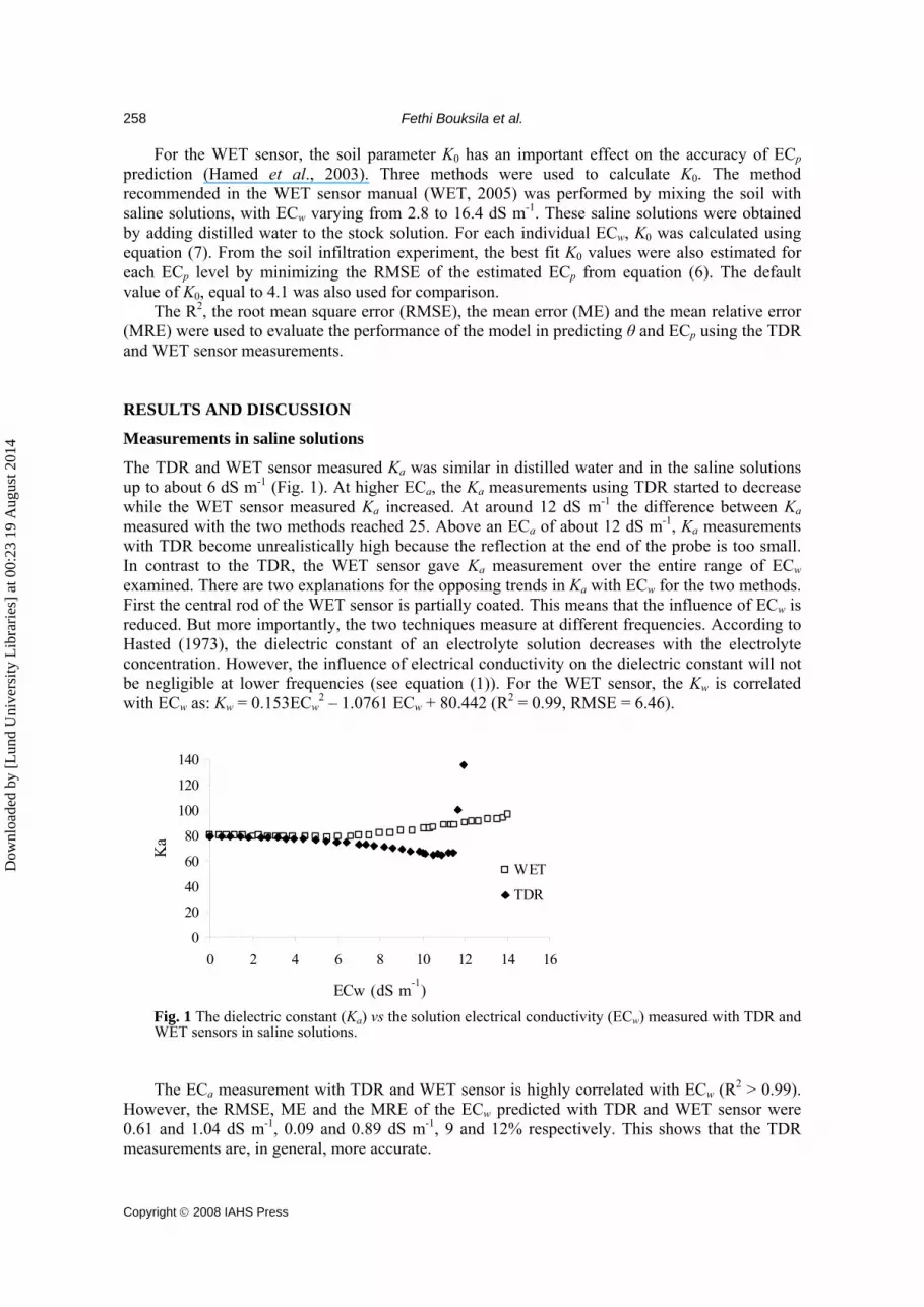
The TDR and WET sensor measured Ka was similar in distilled water and in the saline solutions up to about 6 dS m-1 (Fig. 1). At higher ECa, the Ka measurements using TDR started to decrease while the WET sensor measured Ka increased. At around 12 dS m-1 the difference between Ka measured with the two methods reached 25. Above an ECa of about 12 dS m-1, Ka measurements with TDR become unrealistically high because the reflection at the end of the probe is too small. In contrast to the TDR, the WET sensor gave Ka measurement over the entire range of ECw examined. There are two explanations for the opposing trends in Ka with ECw for the two methods. First the central rod of the WET sensor is partially coated. This means that the influence of ECw is reduced. But more importantly, the two techniques measure at different frequencies. According to Hasted (1973), the dielectric constant of an electrolyte solution decreases with the electrolyte concentration. However, the influence of electrical conductivity on the dielectric constant will not be negligible at lower frequencies (see equation (1)). For the WET sensor, the Kw is correlated with ECw as: Kw = 0.153ECw
2 – 1.0761 ECw + 80.442 (R2 = 0.99, RMSE = 6.46).
0
20
40
60
80
100
120
140
0 2 4 6 8 10 12 14 16
ECw (dS m-1)
Ka
WET
TDR
Fig. 1 The dielectric constant (Ka) vs the solution electrical conductivity (ECw) measured with TDR and WET sensors in saline solutions.
The ECa measurement with TDR and WET sensor is highly correlated with ECw (R2 > 0.99). However, the RMSE, ME and the MRE of the ECw predicted with TDR and WET sensor were 0.61 and 1.04 dS m-1, 0.09 and 0.89 dS m-1, 9 and 12% respectively. This shows that the TDR measurements are, in general, more accurate.
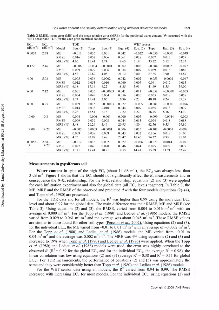
Table 3 RMSE, mean error (ME) and the mean relative error (MRE) for the predicted water content (θ) measured with the WET sensor and TDR for the each pore electrical conductivity (ECp).
Water content In spite of the high ECp (about 14 dS m-1), the ECa was always less than 3 dS m-1. Figure 1 shows that the ECa should not significantly affect the Ka measurements and in consequence the θ–Ka relationship. For the θ–Ka relationship, equations (2) and (3) were applied for each infiltration experiment and also for global data (all ECw levels together). In Table 3, the ME, MRE and the RMSE of the observed and predicted θ with the four models (equations (2)–(4), and Topp et al., 1980) are presented. For the TDR data and for all models, the R2 was higher than 0.99 using the individual ECw level and about 0.97 for the global data. The main difference was their RMSE, ME and MRE (see Table 3). Using equations (2) and (3), the RMSE, varied from 0.004 to 0.016 m3 m-3 with an average of 0.009 m3 m-3. For the Topp et al. (1980) and Ledieu et al. (1986) models, the RMSE varied from 0.029 to 0.061 m3 m-3 and the average was about 0.045 m3 m-3. These RMSE values are similar to those found for other soil types (Persson et al., 2002). Using equations (2) and (3), for the individual ECw, the ME varied from –0.01 to 0.01 m3 m-3 with an average of –0.0002 m3 m-3. For the Topp et al. (1980) and Ledieu et al. (1986) models, the ME varied from –0.01 to 0.04 m3 m-3 and the average was 0.002 m3 m-3. The MRE was 4% using equations (2) and (3) and increased to 19% when Topp et al. (1980) and Ledieu et al. (1986) were applied. When the Topp et al. (1980) and Ledieu et al. (1986) models were used, the error was highly correlated to the observed θ (R2 = 0.89 for the global ECw and for the individual ECw, the average R2 = 0.98), the linear correlation was low using equations (2) and (3) (average R2 = 0.38 and R2 = 0.11 for global ECw). For TDR measurements, the performance of equations (2) and (3) was approximately the same and they were considerably better than Topp et al. (1980) and Ledieu et al. (1986) models. For the WET sensor data using all models, the R2 varied from 0.94 to 0.99. The RMSE increased with increasing ECw for most models. For the individual ECw, using equations (2) and
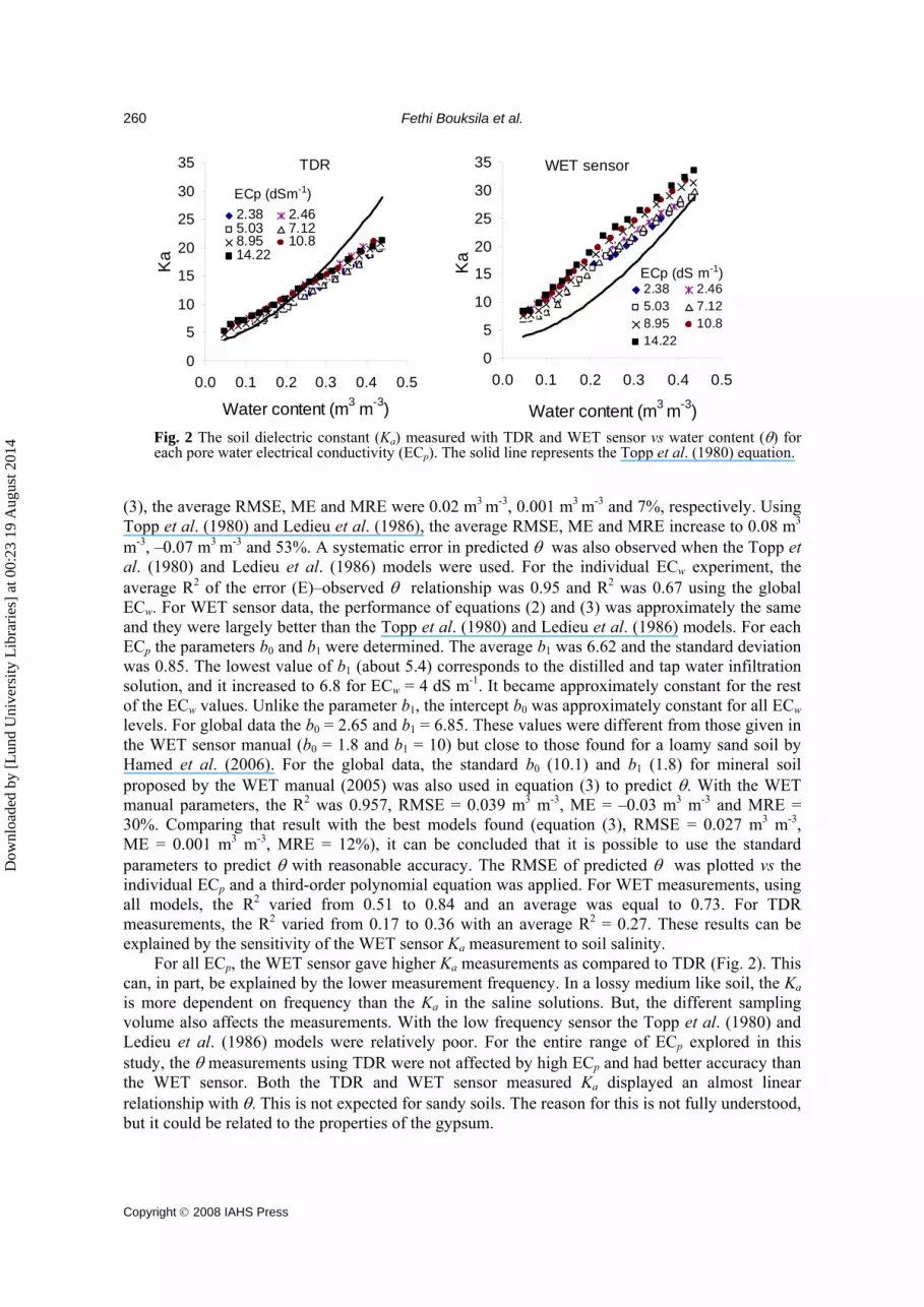
Fig. 2 The soil dielectric constant (Ka) measured with TDR and WET sensor vs water content (θ) for each pore water electrical conductivity (ECp). The solid line represents the Topp et al. (1980) equation.
(3), the average RMSE, ME and MRE were 0.02 m3 m-3, 0.001 m3 m-3 and 7%, respectively. Using Topp et al. (1980) and Ledieu et al. (1986), the average RMSE, ME and MRE increase to 0.08 m3
m-3, –0.07 m3 m-3 and 53%. A systematic error in predicted θ was also observed when the Topp et al. (1980) and Ledieu et al. (1986) models were used. For the individual ECw experiment, the average R2 of the error (E)–observed θ relationship was 0.95 and R2 was 0.67 using the global ECw. For WET sensor data, the performance of equations (2) and (3) was approximately the same and they were largely better than the Topp et al. (1980) and Ledieu et al. (1986) models. For each ECp the parameters b0 and b1 were determined. The average b1 was 6.62 and the standard deviation was 0.85. The lowest value of b1 (about 5.4) corresponds to the distilled and tap water infiltration solution, and it increased to 6.8 for ECw = 4 dS m-1. It became approximately constant for the rest of the ECw values. Unlike the parameter b1, the intercept b0 was approximately constant for all ECw levels. For global data the b0 = 2.65 and b1 = 6.85. These values were different from those given in the WET sensor manual (b0 = 1.8 and b1 = 10) but close to those found for a loamy sand soil by Hamed et al. (2006). For the global data, the standard b0 (10.1) and b1 (1.8) for mineral soil proposed by the WET manual (2005) was also used in equation (3) to predict θ. With the WET manual parameters, the R2 was 0.957, RMSE = 0.039 m3 m-3, ME = –0.03 m3 m-3 and MRE = 30%. Comparing that result with the best models found (equation (3), RMSE = 0.027 m3 m-3, ME = 0.001 m3 m-3, MRE = 12%), it can be concluded that it is possible to use the standard parameters to predict θ with reasonable accuracy. The RMSE of predicted θ was plotted vs the individual ECp and a third-order polynomial equation was applied. For WET measurements, using all models, the R2 varied from 0.51 to 0.84 and an average was equal to 0.73. For TDR measurements, the R2 varied from 0.17 to 0.36 with an average R2 = 0.27. These results can be explained by the sensitivity of the WET sensor Ka measurement to soil salinity. For all ECp, the WET sensor gave higher Ka measurements as compared to TDR (Fig. 2). This can, in part, be explained by the lower measurement frequency. In a lossy medium like soil, the Ka is more dependent on frequency than the Ka in the saline solutions. But, the different sampling volume also affects the measurements. With the low frequency sensor the Topp et al. (1980) and Ledieu et al. (1986) models were relatively poor. For the entire range of ECp explored in this study, the θ measurements using TDR were not affected by high ECp and had better accuracy than the WET sensor. Both the TDR and WET sensor measured Ka displayed an almost linear relationship with θ. This is not expected for sandy soils. The reason for this is not fully understood, but it could be related to the properties of the gypsum.
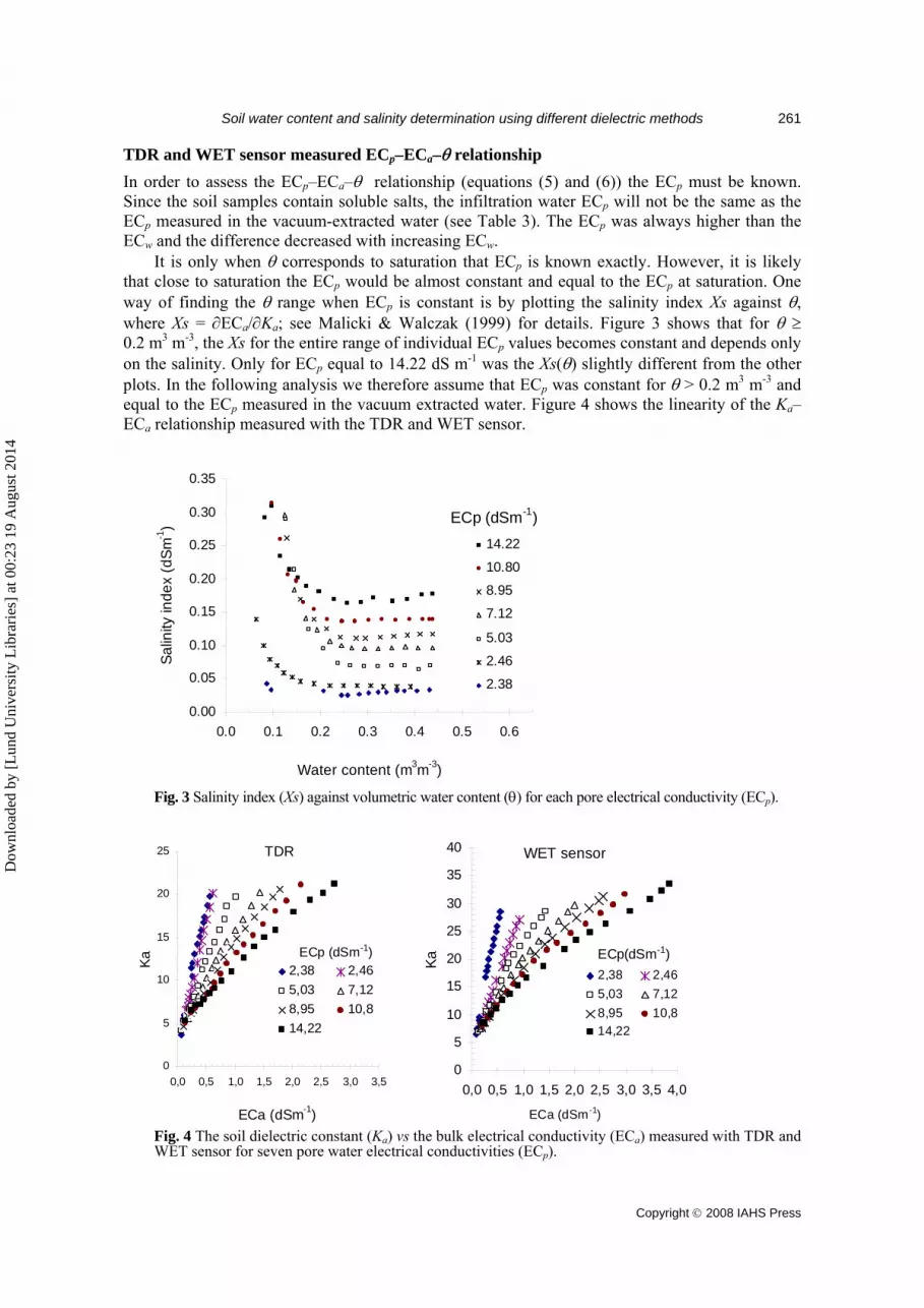
TDR and WET sensor measured ECp–ECa–θ relationship In order to assess the ECp–ECa–θ relationship (equations (5) and (6)) the ECp must be known. Since the soil samples contain soluble salts, the infiltration water ECp will not be the same as the ECp measured in the vacuum-extracted water (see Table 3). The ECp was always higher than the ECw and the difference decreased with increasing ECw. It is only when θ corresponds to saturation that ECp is known exactly. However, it is likely that close to saturation the ECp would be almost constant and equal to the ECp at saturation. One way of finding the θ range when ECp is constant is by plotting the salinity index Xs against θ, where Xs = ∂ECa/∂Ka; see Malicki & Walczak (1999) for details. Figure 3 shows that for θ ≥ 0.2 m3 m-3, the Xs for the entire range of individual ECp values becomes constant and depends only on the salinity. Only for ECp equal to 14.22 dS m-1 was the Xs(θ) slightly different from the other plots. In the following analysis we therefore assume that ECp was constant for θ > 0.2 m3 m-3 and equal to the ECp measured in the vacuum extracted water. Figure 4 shows the linearity of the Ka–ECa relationship measured with the TDR and WET sensor.
0.00
0.05
0.10
0.15
0.20
0.25
0.30
0.35
0.0 0.1 0.2 0.3 0.4 0.5 0.6
Water content (m3m-3)
Salin
ity in
dex
(dSm
-1)
14.22
10.80
8.95
7.12
5.03
2.46
2.38
ECp (dSm-1)
Fig. 3 Salinity index (Xs) against volumetric water content (θ) for each pore electrical conductivity (ECp).
0
5
10
15
20
25
0,0 0,5 1,0 1,5 2,0 2,5 3,0 3,5
ECa (dSm-1)
Ka 2,38 2,465,03 7,128,95 10,814,22
ECp (dSm-1)
TDR
0
5
10
15
20
25
30
35
40
0,0 0,5 1,0 1,5 2,0 2,5 3,0 3,5 4,0
ECa (dSm-1)
Ka
2,38 2,465,03 7,128,95 10,814,22
ECp(dSm-1)
WET sensor
Fig. 4 The soil dielectric constant (Ka) vs the bulk electrical conductivity (ECa) measured with TDR and WET sensor for seven pore water electrical conductivities (ECp).
Table 4 The RMSE, ME and MRE for observed and predicted ECp with the Hilhorst (2000) model using different K0 values; standard value K0 = 4.1; best fit; K0 = f(ECa) from equation (7). For the TDR measurements, the Malicki & Walczak (1999) model was also used, both using standard parameters and parameters adjusted to fit data. ECp 2.38– Model (dS m-1)
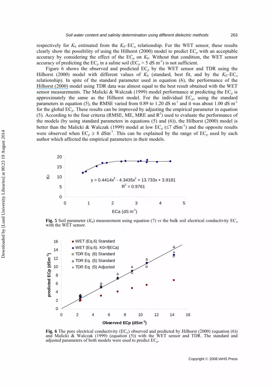
MRE (%) 4.1 28.2 9.3 8.5 6.1 6.2 5.0 8.3 For the TDR measurements, the Hilhorst (2000) and Malicki & Walczak (1999) models were applied and compared. In equation (6), only the standard K0 value (= 4.1) was used since it proved to give accurate ECp predictions. In equation (5), the ECp was calculated using both the standard parameters and adjusted parameters to fit our data. The result is presented in Table 4. The table also shows results of estimating K0 using equation (6), the RMSE, ME and MRE of estimated ECp for the WET sensor measurements. Using WET sensor measurements, whatever method used, K0 increases with ECp up to about 8 dS m-1. At higher ECp it becomes more or less constant. For the individual and the global ECp, the RMSE and the ME of the ECp predicted by equation (6) increases with increase in electrical conductivity of the moistening solution (ECw). In the Hilhorst (2000) model, the K0 value had an important impact on the accuracy of predicted ECp. When the default K0 value (= 4.1) was used, the RMSE, ME and MRE increased from 0.40 to 8.01 dS m-1, from 0.39 to 7.98 dS m-1 and from 28% to 56% for tap water and for ECp equal to 14.22 dS m-1, respectively. The poor accuracy of the Hilhorst (2000) model can be improved by a soil specific calibration of K0. For each individual ECp, the best fit K0 was calculated from equation (6). The RMSE, ME and MRE of the observed and predicted ECp decreased and varied from 0.12 to 2.93 dS m-1, from 0.04 to 1.96 and from 4 to 28%, respectively. These error parameters (RMSE or ME or MRE) were highly correlated to the observed ECp; the R2 of the linear regression was superior to 0.97 using the standard K0 value (= 4.1) and 0.91 using the best fit in the Hilhorst (2000) model. Since our measurements showed that K0 was not constant but depended on ECp we tried a modified Hilhorst model with K0 as a function of ECp. In Fig. 5 the K0 estimated using the method described in the manual is plotted against ECa. A third-order polynomial equation fitted the K0–ECa relationship rather well (R2 ≥ 0.90). That equation was used in equation (6) to predict ECp. For the individual ECp levels, using this modified Hilhorst model, the RMSE varied from 0.11 to 0.92 dS m-1, the ME from –0.45 to 0.48 dS m-1 and the MRE varied from 4 to 28% with an average equal to about 10%. For the global range of ECp, the RMSE was 4.15 dS m-1, ME = 3.27 dS m-1 and MRE = 40 % using the standard K0 and they decreased to 0.68 dS m-1, 0.20 dS m-1 and 8%
Dow
nloa
ded
by [
Lun
d U
nive
rsity
Lib
rari
es]
at 0
0:23
19
Aug
ust 2
014
Soil water content and salinity determination using different dielectric methods
respectively for K0 estimated from the K0–ECa relationship. For the WET sensor, these results clearly show the possibility of using the Hilhorst (2000) model to predict ECp with an acceptable accuracy by considering the effect of the ECp on K0. Without that condition, the WET sensor accuracy of predicting the ECp in a saline soil (ECp > 5 dS m-1) is not sufficient. Figure 6 shows the observed and predicted ECp by the WET sensor and TDR using the Hilhorst (2000) model with different values of K0 (standard, best fit, and by the K0–ECa relationship). In spite of the standard parameter used in equation (6), the performance of the Hilhorst (2000) model using TDR data was almost equal to the best result obtained with the WET sensor measurements. The Malicki & Walczak (1999) model performance at predicting the ECp is approximately the same as the Hilhorst model. For the individual ECp, using the standard parameters in equation (5), the RMSE varied from 0.89 to 1.20 dS m-1 and it was about 1.00 dS m-1 for the global ECp. These results can be improved by adjusting the empirical parameter in equation (5). According to the four criteria (RMSE, ME, MRE and R2) used to evaluate the performance of the models (by using standard parameters in equations (5) and (6)), the Hilhorst (2000) model is better than the Malicki & Walczak (1999) model at low ECp (≤7 dSm-1) and the opposite results were observed when ECp ≥ 8 dSm-1. This can be explained by the range of ECp used by each author which affected the empirical parameters in their models.
Fig. 6 The pore electrical conductivity (ECp) observed and predicted by Hilhorst (2000) (equation (6)) and Malicki & Walczak (1999) (equation (5)) with the WET sensor and TDR. The standard and adjusted parameters of both models were used to predict ECp.
In the present study, the TDR and FDR (WET sensor) techniques were explored and compared in both saline solutions and in a saline gypsum soil. In the saline solutions, the TDR measured Ka and ECa gave better accuracy than the WET sensor equivalent up to an ECa level of about 11 dS m-1. At higher ECa the TDR measurements became unrealistic. The WET sensor was less affected by high ECa and gave reasonable Ka measurements for all ECa levels. Measurements were taken in loamy sand with about 65% gypsum. Seven moistening solutions with ECw varying from 0 to 14 dS m-1 were used to explore the performance and limits of TDR and WET sensors for predicting θ and ECp. The WET sensor gave higher Ka values than the TDR. Because of the low frequency of the FDR and the coated rod probe, it seems that the Topp et al. (1980) and Ledieu et al. (1986) models cannot be recommended for the WET sensor. With these models, the RMSE and the MRE of the observed and predicted θ were about 0.04 m3 m-3 and 19% for TDR and 0.08 m3 m-3 and 54% for WET sensor measurements, respectively. For the TDR measurements and global ECp, the RMSE was 1.16 and 0.99 dS m-1 and the MRE was 14% and 19% for the Hilhorst (2000) and Malicki & Walczak (1999) models respectively. The accuracy of the WET sensor to predict the ECp was very poor using the standard value of K0. For the individual ECp levels the RMSE and the MRE of the predicted ECp varied from 0.40 to 8.01 dS m-1 and from 25 to 56% respectively. The errors in the ECp predictions were highly correlated to the ECp (R2 ≥ 0.97). For the global (all ECp levels together) ECp, the RMSE was 4.15 dS m-1 and the MRE was 40%. The K0 was not constant but increased with ECp. By replacing the standard K0 by a third-order polynomial K0–ECa relationship, the RMSE instead varied from 0.11 to 0.92 dS m-1 and the MRE varied from 4 to 28% for the individual ECp. For the global data, the RMSE was 0.68 dS m-1 and the MRE was 8%. Further studies will focus on the impact of the residual gypsum salt and ECp on θ, ECa and ECp. Measurements will be conducted in several soils with different gypsum content and soil particle size. REFERENCES
Bouksila, F., Bahri, A. & Ben Issa, I. (2006) Gestion de l’eau, drainage et salinité dans les oasis du sud tunisien. Rapport d´activités de recherche. Institut National de Recherche en Genie Rural, Eau et Forets, Tunis, Tunisie.
Cosenza, P. & Tabbagh, A. (2004) Electromagnetic determination of clay water content: role of the microporosity. Clay Sci. 26, 21–36.
Dalton, F. N. (1992) Development of time-domain reflectrometry for measuring soil water content and bulk soil electrical conductivity. In: Advances in Measurement of Soil Physical Properties: Bringing Theory into Practice (ed. by G. C. Topp & W. D. Reynolds), 143–167. SSSA Spec. Publ. no. 30, Soil Science Society of America, Inc., Madison, Wisconsin, USA.
Escudero, A., Iriondo, J. M., Olano, J. M., Rubio, A. & Somolinos, R. C. (2000) Factors affecting establishment of a gypsophyte: the case of Lepidium subulatum (Brassicaceae). Am. J. Botany 87(6), 861–871.
FAO (1990) Management of Gypsiferous Soils. FAO Soils Bulletin 62, Rome, Italy. Hamed, Y., Persson, M. & Berndtsson, R. (2003) Soil solution electrical conductivity measurements using different dielectric
techniques. Soil Sci. Soc. Am. J. 67, 1071–1078. Hamed, Y., Samy, G. & Persson, M. (2006) Evaluation of the WET sensor compared to time domain reflectometry. Hydrol. Sci.
J. 51, 671–681. Hasted, J. B. (1973) Aqueous Dielectrics. Chapman & Hall, London, UK. Heimovaara, T. J. (1993) Time domain reflectometry in soil science: theoretical backgrounds, measurements and models. PhD
Thesis, University of Amsterdam, The Netherlands. Hilhorst, M. A. (2000) A pore water conductivity sensor. Soil Sci. Soc. Am. J. 64, 1922–1925. Keren, R., Kreit, J. F. & Shainberg, I. (1980) Influence of size of gypsum particles on the hydraulic conductivity of soils. Soil
Sci. 130, 113–117. Ledieu, J., De Ridder, P., De Clerck, P. & Dautrebande, S. (1986) A method of measuring soil moisture by time-domain
reflectometry. J. Hydrol. 88, 319–328. Malicki, M. A. & Walczak, R. T. (1999) Evaluating soil salinity status from bulk electrical conductivity and permittivity. Eur.
J. Soil Sci. 50, 505–514. Malicki, M. A., Plagge, R. & Roth, C. H. (1996) Improving the calibration of dielectric TDR soil moisture determination taking
into account the solid soil. Eur. J. Soil Sci. 47, 357–366.
Dow
nloa
ded
by [
Lun
d U
nive
rsity
Lib
rari
es]
at 0
0:23
19
Aug
ust 2
014
Soil water content and salinity determination using different dielectric methods
Malicki, M. A., Walczak R. T., Kock, S. & Fluhler, H. (1994) Determining soil salinity from simultaneous readings of its electrical conductivity and permittivity using TDR. In: Proc. Symp. on Time Domain Reflectometry in Environmental, Infrastructure, and Mining Applications (ed. by K. M. O’Connor, C. H. Dowding & C. C. C. Jones) (Evanston, Illinois, USA, September, 1994), 328–336. Special Publication SP 19-94, NTIS PB95-105789. US Bureau of Mines, Minneapolis, Minnesota, USA.
Mojid, M. A, Wyseure, G. C. L. & Rose, D. A. (1998) The use of insulated time-domain reflectometry sensors to measure water content in highly saline soils. Irrig. Sci. 18, 55–61.
Nadler, A., Gamliel, A. & Peretz, I. (1999) Practical aspects of salinity effect on TDR-measured water content: a field study. Soil Sci. Soc. Am. J. 63, 1070–1076.
Persson, M. (1997) Soil solution electrical conductivity measurements under transient conditions using TDR. Soil Sci. Soc. Am. J. 61, 997–1003.
Persson, M. (2002) Evaluating the linear dielectric constant-electrical conductivity model using time domain reflectometry. Hydrol. Sci. J. 47, 269–278.
Persson, M. & Berndtsson, R. (1998) Texture and electrical conductivity effects on temperature dependency in time domain reflectometry. Soil Sci. Soc. Am. J. 62, 887–893.
Persson, M., Berndtsson, R., Nasri, S., Albergel, J., Zante, P. & Yumegaki, Y. (2000) Solute transport and water content measurements in clay soils using time domain reflectometry. Hydrol. Sci. J. 45, 833–847.
Persson, M., Sivakumar, B., Berndtsson, R., Jacobsen, O. H. & Schjønning, P. (2002) Predicting the dielectric constant-water content relationship using artificial neural networks. Soil Sci. Soc. Am. J. 66, 1424–1429.
Pouget, M. (1965) Mesures d’´humidité sur des échantillons de sols gypseux. Cah. ORSTOM, série Pédol. 3(2), 139–148. Pouget, M. (1968) Contribution à l’étude des croûtes et encroutement gypseux de nappe dans le sud-tunisien. Cah. ORSTOM,
série Pédol. 6(3). Rhoades, J. D., Ratts, P. A. & Prather, R. J. (1976) Effects of liquid-phase electrical conductivity, water content, and surface
conductivity on bulk soil electrical conductivity. Soil Sci. Soc. Am. J. 40, 651–655. Topp, G. C., Davis, J. L. & Annan, A. P. (1980) Electromagnetic determination of soil water content: measurements in coaxial
transmission lines. Water Resour. Res. 16, 574–582. Topp, G. C., Yanuka, M., Zebchuk, W. D. & Zegelin, S. (1988) Determination of electrical conductivity using time domain
reflectometry: soil and water experiments in coaxial lines. Water Resour. Res. 24, 945–952. USDA (1954) Diagnostic and improvement of saline and alkali soil. Agriculture Handbook No. 60, US Dept. of Agriculture. Vieillefon, J. (1979) Contribution à l’amélioration de l’étude analytique des sols gypseux. Cah. ORSTOM, série Pédol. 17(3),
195–223. WET (2005) User Manual for the WET Sensors; Type WET-2, Version 1.3. Delta-T Devices Ltd, Cambridge, UK. http://www.delta-t.co.uk. Received 30 October 2006; accepted 29 August 2007