Species composition, diversity, biomass and production of the benthic invertebrate community of the...

Not to be quoted without prior reference to the authors © Crown Copyright 2007

Fisheries Research Services Internal Report No: 20/07

SPECIES COMPOSITION, DIVERSITY, BIOMASS AND PRODUCTION OF THE EPIBENTHIC INVERTEBRATE COMMUNITY OFF THE SCOTTISH WEST COAST

H M Fraser, S P R Greenstreet, M R Robertson, N Jacob and L A Robinson

May 2007

Fisheries Research Services Marine Laboratory 375 Victoria Road Aberdeen AB11 9DB

Species Composition, Diversity, Biomass and Production of the Epibenthic Invertebrate Community

1

SPECIES COMPOSITION, DIVERSITY, BIOMASS AND PRODUCTION OF THE EPIBENTHIC INVERTEBRATE COMMUNITY OFF THE SCOTTISH WEST

COAST

Fraser, H. M., Greenstreet, S. P. R., Robertson, M. R., Jacob, N. and Robinson, L. A.

Fisheries Research Services, Marine Laboratory, 375 Victoria Road, Aberdeen, AB11 9DB

1.1. INTRODUCTION The epibenthos are the component of the benthic invertebrate community that spend the majority of their lifecycle living in close association with the surface of the seafloor. In recent years many large scale benthic diversity surveys have been undertaken in the seas surrounding the UK. The North Sea has been extensively examined by Basford et al., (1989); Callaway et al., 2002; Eleftheriou & Basford (1989) and Zűlke et al., (2001) while work was carried out in the Irish Sea by Swift (1993); Hensley (1996) and Ellis et al., (2000). By comparison, the benthic faunal diversity off the Scottish west coast has received very little attention. Pinn & Robertson (2003) investigated the macro-infaunal communities found in the Greater Minch area on the Scottish west coast using RoxAnn© and related these to sediment type but other than that, no other large scale diversity studies have been undertaken along the Scottish west coast. The purpose of this report is to present the findings of the epibenthic surveys that have been undertaken as part of the ROAME – MF0753 Managing Fisheries to Conserve Groundfish and Benthic Invertebrate Species Diversity. This project links the characteristics of the benthic invertebrate communities to demersal fish diversity on the Scottish west coast. As part of this development, methods for estimating secondary production from the size-structured epibenthic community have also been explored, as this is an important link to the overlying demersal fish community. 1.1.1. Catchability issues In attempting to describe the epifaunal community in terms of its composition, diversity, and productivity, it is important to take account of the restrictions that the sampling procedure has on the community being represented. The impressions of the epibenthic community gained from the analysis of our sample data is not that of the actual epifaunal community present at each sampled location. Instead it is a view of the community biased by the differential selectivity of the sampling gear for each species present at each location. No trawl gear ever samples all the individuals present in the path of the net. Trawling is a selective process because the catch rates of different species in any given sampling gear vary considerably, both between species and between size classes of the same species. Many factors can be involved. Although many of the epibenthic species sampled are less motile than the fish species sampled in the fish surveys, it is likely that a proportion of the more mobile species can move out of the way of the gear. Also, some of the species live partially submerged in the sediment during certain times of the day and these too may not be sampled well by a towed trawling gear. Infact, it is likely that catchability of the epibenthic community in the 2-metre beam trawl varies as a result of a number of factors including motility, size and living position on/within the seafloor. Because there have been few large-scale epibenthic surveys to date, there is little information available to account for catchability issues. Based on the


2

findings of a recent study, we have examined this issue and discuss the implications of the results on epifaunal community analyses (Reiss et al., 2006). 1.1.2. Sampling effort issues Any analyses involving species diversity, must take account of the influence of sampling effort on index performance. Previous explorations of variation in species diversity of macrofaunal invertebrates have tried to standardise for sampling effort effects on diversity indices, by calculating diversity based on an arithmetic mean of a number of iterations of the indices for a given abundance of animals randomly selected from the sample (Heip et al., 1992). However, these methods do not account for the inherent influence of abundance on the indices and the fact that both this and species number will continue to increase up to a given sampled area (Colwell & Coddington 1994; Connor et al., 2000; Gotelli & Colwell 2001; van Gemerden et al., 2005). Preliminary analysis of the relationship between index value and variation in sampling effort is a critical first step to determine at what sampling effort level index values stabilize, and thus begin to represent the true community diversity rather than just being a consequence of the level of sampling effort. Previous attempts to determine the number of 2-metre beam trawl samples required to represent community diversity of an ICES rectangle suggest that not only do you need greater than 5 replicate tows, but that the number of tows required varies depending on: the index of diversity used (i.e. species number Vs. indices of dominance and evenness), species group considered (i.e. sessile vs. free-living epifauna) and the geographical area studied. 1.1.3. Productivity Traditional methods for calculating secondary production from the benthos have been applied to single animals or populations based on the change in body mass or growth over time. However, the methods used to calculate this generally involve the destruction of samples and requires intensive sampling of the same population to account for changes over time. Methods include those based on cohort analysis, size class based methods and the relationship between productivity and mortality (Cushman et al., 1978; Wildish & Peer, 1981; Crisp, 1984; Morin et al., 1987). None of these methods are practical when trying to quantify secondary production at the community level. During the ROAME project, assessment of spatial variation in secondary production from the epifaunal benthos at between 20 and 25 stations per year in waters west of Scotland over four years has been undertaken. Over the last 20 years, efforts have turned towards parameterising empirical models that can be used to estimate secondary production (Brey, 2002). These models describe the relationships between easily measured parameters such as biomass, individual body mass and water temperature with production (P) or the production/biomass (P/B) ratio for individual populations. Empirical relationships between these parameters are calculated using the combined published results of the traditional studies as described above. It is then possible to predict P or the P/B ratio for new sampled populations just using data for the easily measured parameters such as biomass and temperature. All of these approaches depend more or less directly on the negative exponential relationship between metabolic rate and body mass. The earliest empirical models related the P/B ratio to one parameter. For example, the P/B ratio was related to lifespan by Robertson (1979), to adult body mass (at maturity) by Banse & Mosher (1980) and to mean individual body mass by Schwinghamer et al. (1986). Two-parameter models were published by Brey (1990) (P vs. biomass and mean individual body mass) and by Edgar (1990a, 1990b) (P vs. mean individual body mass and bottom water temperature). Even more complex three-parameter models were published by Morin & Mourassa (1992), who related


3

production of stream benthos to biomass, mean body mass and annual mean water temperature; Plante and Downing (1989), who related production of lake benthos to biomass, maximum body mass, and surface water temperature, and; Tumbiolo & Downing (1994), who related production of marine benthos to biomass, maximum body mass, surface water temperature and water depth. More recent models have generally all included environmental parameters (usually water temperature and sometimes depth) in recognition of the influence of these on growth rates and thus also productivity. Brey et al., (1996) and Brey (1999) unified all previous habitat-specific approaches into one large model for macrofaunal benthos in general. In Brey et al., (1996) "Artificial Neural Networks" were trained to estimate P/B from body mass, taxon, mode of living, water temperature and water depth and it is suggested that this approach performs slightly better than the usual multiple linear models. The latest models are available on a website maintained by Brey (2002). Here the relationships are updated regularly to include any new field studies of direct measurements of population production and P/B ratios, thus increasing the number of studies that the empirical model is based on. In all cases, models are based on data for individual species populations. Thus production is calculated for each species making up a community and all species totals are then summed to give total community production. Where species level data do not exist, the variability around mean individual weight will be likely to increase as taxonomic resolution decreases and this may affect the validity of using the empirical models that include mean individual weight as a parameter. However, here the epibenthic data have been size structured to reduce the variability around the mean individual weight per species. When carrying out routine, large-scale surveys such as those undertaken in this project, it may not be feasible to work up the data to species level. In this project we examined the methods available for estimating secondary productivity from the epifauna. The epifauna include both colonial and individual based populations of animals. Due to this it was necessary to combine a number of methods, some based on biomass, some based on size-classed individuals grouped based on their individual weights and some based on average mean weight.

1.2. METHODS 1.2.1. Data set One beam trawl tow was taken at each station sampled, close to the track of the main demersal fish-sampling trawl. Overall 92 2-metre beam trawl samples were taken to the west of Scotland, 19 in 2001, 27 in 2002, 21 in 2003 and 25 in 2004 (Figure 1.2.1.1). Sampling was undertaken between November and December in each year. All samples were taken with a 2-m beam trawl constructed from galvanised steel, fitted with a 20mm mesh (10mm knot to knot) and a liner of 4mm knotless mesh (2mm ‘knot to knot’) (a detailed description of the specifications can be found in Jennings et al., 1999). The beam trawl was shot with a warp length of approximately three times water depth and towed at between 1-1.5 knots for 5 minutes. Where possible, a Scanmar© depth unit (which shows when the trawl reaches and leaves the seabed) was attached to allow accurate timing of the duration of beam trawl fishing.


4

53

54

55

56

57

58

59

60

Deg

rees

Lat

itude

-12 -10 -8 -6 -4 -2

Degrees longitude

49

48

47

46

45

44

43

42

41

40

39

38

37

36

35

E7E6E5E4E3E2E1E0D9D8

Figure 1.2.1.1. All 92 stations sampled for epifauna with a 2-metre beam trawl during the 2001 to 2004 west coast surveys. 1.2.2. Sample treatment Samples were washed through a 5mm and 2mm sieve (internal mesh size) and epibenthic invertebrates and fish separated from the remains. For those animals retained in the 5mm sieve the majority of species were identified, measured and weighed (blotted wet weight) onboard. Sessile animals were recorded as present or absent with a total weight given where possible. Weights were taken using a seagoing marine scale (Pols) with an accuracy of 0.01g. For those species that were either too small to be accurately weighed onboard, or too difficult to identify without a microscope, specimens were preserved in 4% buffered formaldehyde and returned to the laboratory. Species identification was based on Haywood & Ryland (1990), a number of specialised identification keys, and a digital identification key (SID) developed under EC FAIR project CT 95-0817. Specimens that individual partners had found difficult to identify were examined at a workshop held six months after the surveys at the Senckenburg Institute, Germany. All names were standardised to the nomenclature of Howson & Picton (1999) and where more recent changes in nomenclature have occurred, or new species found, a record was made. All specimens in the 5mm-sieve fraction were identified to the lowest taxonomic level. Demersal fish caught in the 2m-beam trawl samples are not considered further in the analysis of the epibenthos, but are discussed in section 1.3.6.


5

1.2.3. Defining “Standard Samples” Despite fairly rigid protocols being laid down for each survey, the trawl samples contained were not fully standardized. Trawls were expected to be over 5min, because the actual trawl duration was taken as the time between the trawl starting to tow on the seafloor and the time when the trawl had lifted off the seafloor (this could be several minutes after the 5min timed tow). However, some trawls were greater than 2min over the standardised tow time. Maximum tow duration in the database was 8.28min. Average tow duration of all tows of 5min duration and less than 8.28min duration was 6min. Table 1.2.3.1 shows the summary statistics for all the 2m beam trawls carried out on the west coast from 2001 to 2004. Statistic MAFCONS 2m Beam trawl (m2) Number trawls 92 Mean 663.88 Standard Deviation 182.99 Lower 5% range point 503.78 Upper 5% range point 868.37 Table 1.2.3.1 Trawl swept-area statistics for MAFCONS 2metre beam trawl samples with actual trawl distance recorded (using Scanmar) for all trawls. 1.2.4. Catchability of the gear Catchability of the gear affects interpretation of all analyses because it has a direct effect on both the number of species caught, and the number and biomass of individuals caught of each species. Ideally all catch data should be raised to account for catchability. However, in order to calculate catchability it is necessary to compare abundances reported by the survey gear with a reliable independent estimate of the total abundances of the species caught. There are no independent estimates of the abundance of any epifauna species on the Scottish west coast currently available (other than some estimates for a small number of commercial shellfish stocks - see references in Reiss et al., 2006). Previous studies have compared either: the catch from the 2metre beam trawl with other samplers, such as the 3 metre beam trawl and the anchor dredge, or the catchability of the 2 metre beam trawl as a function of the total catch of a number of beam trawls towed directly after each other (Reiss et al., 2006). Clearly these results do not give an absolute catchability value, and those species not sampled by any of the gears examined will not be covered at all, but they do provide interesting results in terms of the magnitude of underestimation encountered and how this varies between different taxa and different habitats. Reiss et al., (2006) calculated catching efficiency for all taxa combined and the individual invertebrate taxa that had at least 10 individuals in the first trawl, by comparing the values for the first of three beam trawls towed directly behind each other with the total values for all three combined. In this study the potential to apply catchabilities determined by Reiss et al., (2006) to the MAFCONS 2-metre beam trawl dataset was explored. 1.2.5. Distribution of abundance and biomass For each station, total abundance (N) (not including colonial species) and total biomass (B) (including all species except a small number of encrusting species that could not be weighed) were standardised to densities per m2 by dividing the biota totals by the station specific swept area. Swept area was itself calculated by multiplying the total track fished by the width of the beam trawl (two metres). Univariate indices of total abundance and total biomass were calculated for each station as point estimates for each year. Both years were subsequently combined and mean


6

density (N per m2) and biomass calculated for each ICES rectangle using all tows taken in a particular rectangle. Distributions of the 12 dominant species based on total abundance across the survey area (non-colonial species only), and the 12 dominant species based on total biomass across the survey area (including colonial species) were plotted. 1.2.6. Distribution of communities based on relative abundance of species (community composition) In order to enable full analysis where only presence/absence data were available, the fauna were subdivided into two groups – all epifauna (including colonial species – presence/absence analysis) and non-colonial species only (where species abundance (Nm-2) for each station was used as the basic input data). Initially, the Bray-Curtis similarity in species composition between stations was explored separately for each of the four surveys (2001 to 2004). Subsequently, a Bray-Curtis similarity matrix comparing the similarity between the epifauna community species composition present in all pairs of ICES rectangle, was constructed for the combined surveys after first pooling the entire sample data collected for each ICES rectangle. The Bray-Curtis similarity matrices were then subjected to hierarchical group-average clustering to identify the groups of stations within years and ICES rectangles overall with similar species compositions. Species characteristic of these individual community clusters were extracted using the SIMPER routine in PRIMER© (Clarke & Warwick 2001). This examines the percentage contribution of each species to the similarity within the characteristic community group and between different groups. The term ‘characteristic community’ is used here to depict a group of stations with similar epibenthic species composition and does not imply any particular ecological interactions. All abundance data were root-root transformed to down-weight the effect of the most abundant species on the Bray-Curtis similarity indices. All analyses were performed using the PRIMER© software. 1.2.7. Distribution of species diversity Species diversity conceptually consists of two different aspects of species relative abundance; the actual number of species included in any particular sample, and the evenness of the distribution of individuals between the species encountered. Here we use three different metrics each differing in the extent to which they are influenced by one or other of these two aspects of species diversity (Southwood, 1978): Hill’s N0 (the total number of species, or species richness); Hill’s N1 (an index of diversity influenced by species richness defined as expH΄, where H΄ is the Shannon-Wiener index of diversity); and Hill’s N2 (an index of diversity influenced by dominance defined as 1/D, where D is Simpson’s index of diversity). Hill’s N1 is computed as:

)(*

11

sS

ss pLnp

eN∑−== 1.2.7.1.

and Hill’s N2 is computed as:

∑=

= S

ssp

N

1

22

1 1.2.7.2.

where ps is the proportion of the total number of individuals contained in the sample in question contributed by each of the S species recorded in the sample (Magurran, 1988). N1 is more sensitive to the number of species recorded in the sample, where as N2 is more sensitive to the evenness of the distribution of individuals between species. Species richness (Hill’s N0) was broken down to all species (including presence/absence data) and non-colonial species, whilst Hill’s N1 and N2 were calculated using only the non-colonial species data, as they require the individual species abundance values. All diversity metrics were determined using the PRIMER© software package (Clarke & Warwick 2001).


7

1.2.8. Assessing the level of sample aggregation required The number of epibenthic invertebrate samples available for analysis was extremely limited. Analysis of the fish data suggested that at a search radius exceeding 50km, estimates of α diversity started to be confounded by the inclusion of elements of β diversity. Because of their more sedentary nature compared with fish, it was thought that the inclusion of β diversity into estimates of epibenthic α diversity would occur at considerably smaller range than this. Thus, the data for formal evaluation of the levels of sample aggregation required to properly assess epibenthic species richness and diversity were simply not available to this study. Incorporation of the datasets collected as part of the earlier Biodiversity projects would certainly help in this respect, and such analyses may be possible in the future. However, considering the data requirements necessary to assess adequate sampling effort for the fish assemblage, we feel that this would still fall short of what was really necessary. Proper assessment of epibenthic invertebrate assemblage still requires the collection of additional data. For the purposes of this study therefore, we simply aggregated all the epibenthic invertebrate samples available from each of the four years sampling combined and calculated all our statistics for each ICES rectangle. The total area sampled in each rectangle was determined and the effect of sampling effort on all statistic values was assessed. Where significant effects were observed, the values calculated for each ICES rectangle for the statistic in question could then be corrected for variation in sampling effort. 1.2.9. Secondary production All productivity analysis was carried on density data (N.m-2 and kg.m-2). As secondary production from the Scottish west coast survey is based on data only collected at one time of year, it was not possible to use any of the empirical models that also take annual variation in biomass and temperature into account. Jennings et al. (2001) published an empirical relationship between P:B and individual weight but this did not take into account the additional variability associated with temperature and as the MAFCONS project is interested in spatial patterns at the scale of the Scottish west coast, where variation in bottom temperature is considerable, it was considered imperative that temperature be taken into account.

1.2.9.1. Edgar’s Empirical Model Edgar’s (1990a, 1990b) empirical model for epifauna, given by:

( ) ( )LogTLogBLogP 68.078.099.1 ++−= 1.2.9.1.1 is based on the relationship between daily production, mean individual body mass and water temperature, where P is the daily production (μg.day-1), B is the mean individual ash-free dry mass (μg) and T is the bottom water temperature (ºC). The model was developed using a dataset of actual data for all of these parameters from studies of 41 individual species. On examining this relationship, Edgar found that models for mollusca and crustacea separated from other infauna and other epifauna (epifauna equation given above). Thus all the taxa in the epifaunal databases were assigned to any of these four groups before the empirical relationships for each one was applied. For the epifaunal dataset, the data were per species so it was possible to assign these to either epifauna or infauna directly based on knowledge of the living habit of the specific species. If an animal is both epifaunal and infaunal, it was assigned to the living habit for which it was known to spend over 50 % of its time.


8

1.2.9.2. Applying Edgar’s Model to Species with size Structured Data For the majority of species sampled it was possible to individually weigh and measure all individuals. Based on this, a length frequency was constructed for each species in each sample and weight at length relationships determined and used to calculate mean individual weight per size class. Mean individual wet weight in grams was then converted to ash free dry weight (AFDM) in micrograms (Brey, 2002 - see below). Daily production per species was then calculated using mean individual weight and water temperatures recorded on the environmental data sheets at each station. Total daily production per species was calculated by multiplying daily production per mean weight class by the total number of individuals in that weight class and then summing across all size classes within a sample. In some instances size structure data were missing and under these circumstances a mean body mass was assumed, derived from the total sample weight and sampled number of the species in question.

1.2.9.3. Applying Edgar’s Model to Species without size Structured Data but with Abundance and Biomass

For a number of species no individual length and weight data were available, but total abundance and total biomass were and these were used to calculate an individual mean weight. Although this is not as accurate as using individual weights per size category, it is more accurate than using published P:B ratios which only tend to be available for very low taxonomic resolution groups (e.g. Class or Phyla). For each sample, total biomass per species was converted to ash free dry mass (AFDM) using published conversion factors (Brey, 2002 - see below) and the mean individual weight per species calculated using the total number of individuals and total biomass (AFDM). Daily production was then calculated using mean individual weight and water temperatures taken from the environmental data recorded at each station. Total daily production per species was calculated by multiplying daily production per mean weight class by the total number of individuals.

1.2.9.4. Applying Edgar’s Model to Species with only Biomass Data For Edgar’s model either size structured data or at least the total number of individuals and total ash free dry mass (biomass) are required to calculate the mean individual weight required by the empirical relationship. For a number of taxa in the epifaunal database there were no biomass data as the animal encountered was encrusting and thus it could not be weighed. In these cases no production could be calculated. More commonly however, biomass data were available but abundance data were not. This occurred either because animals were colonial (and thus it was not possible to count the number of individuals), or where individual animals were fragmented. In these cases it was not possible to account for production directly by applying Edgar’s model. However, where biomass data were available it was still possible to assign total production using P/B ratios. A P/B ratio was assigned to the taxon group following the steps described below and then biomass multiplied by the ratio to give total daily production. Three different steps were followed to assign P/B ratios to species with only biomass data. Firstly, where a P/B ratio was available for that species, based on survey data at the level of the Phyla this was used. Secondly, where no P/B ratios were available from the survey, but were available in the literature these were assigned. Finally, where no P/B ratios were available for a group (e.g. Bryozoa), the P/B ratio provided by Brey (2002) of 0.012 for miscellaneous benthic invertebrates was applied.


9

1.2.9.5. Converting Wet Mass to Ash Free Dry Mass Using Edgar’s method, all wet mass (WM) biomass values need to be converted to ash free dry mass (AFDM). Brey (2002) gives a table of WM>AFDM conversion factors for invertebrates at the level of taxonomic resolution for which there are sufficient data to assign a value. All conversion factors are based on calculations of the difference between wet mass and ash free dry mass for a number of examples for each group (a full reference list can be obtained from the author). Each species in the epifaunal database was assigned to a corresponding Brey group, but where no corresponding link to a Brey group was available; a number of steps were followed. If no alternative source of conversion factor was available, but it was agreed that a taxon resembled a group with a Brey conversion factor, based on its behaviour in the ashing and drying procedure, this alternative group’s conversion factor was used. For ‘Other organic matter’, where fragments of biomass were found in a sample but it was not possible to assign them to any taxonomic group, the WM>AFDM conversion was a mean of the Mollusca, Echinodermata, Annelida and Crustacea values.

1.2.9.6. Total Daily Community Production Once total daily production had been calculated for each species within a sample following the methods described above, total community production was calculated by summing across all species within a sample.

1.3. RESULTS 1.3.1. Catchability The findings of Reiss et al. (2006) suggest high variability in catching efficiency of a standard 2 - metre beam trawl between species and even within species between different areas. Even between two species of the same genera, Crangon allmanni and Crangon crangon, there was over ten percent difference in catching efficiency at the Box A study site (Table 1.3.1.1.). Between 70% and 76% of the total species caught were caught by the first trawl in Box A and between 54% and 84% in Box N. Box N had a more coarse sandy substratum in comparison to the muddy sand substrate found in Box A. It is suggested that the lower catching efficiency of some of the species described for Box N was due to the lower penetration depth of the gear in coarser sediments (Reiss et al., 2006). Catching efficiency in Box A Catching efficiency in Box N Taxon Abundance (%) Biomass (%) Abundance (%) Biomass (%) Corystes cassivelaunus 64† 55 ± 5 - - Liocarcinus holsatus* 18 ± 5 20 ± 10 9 ± 2 9 ± 3 Pagurus bernhardus - - 51‡ ± 1 64 ± 8 Crangon allmanni* 56 ± 4 58 ± 4 26 ± 8 27 ± 7 Crangon crangon 43 ± 6 40 ± 6 31 ± 7 28 ± 5 Processa spp. 72‡ ± 8 83 ± 24 - - Asterias rubens 42 ± 7 46 ± 8 46 ± 6 53 ± 7 Astropecten irregularis 34 ± 9 34 ± 9 35 ± 10 37 ± 12 Nucula nitidosa 19‡ ± 19 11 ± 16 - - Branchiostoma lanceolata - - 0‡ ± 0 0 ± 0 All taxa 44 ± 5 32 ± 8 36 ± 4 45 ± 9

*Indicates significant differences between sites (see Reiss et al., 2006). †Based on one replicate only; ‡Based on two replicates only.


10

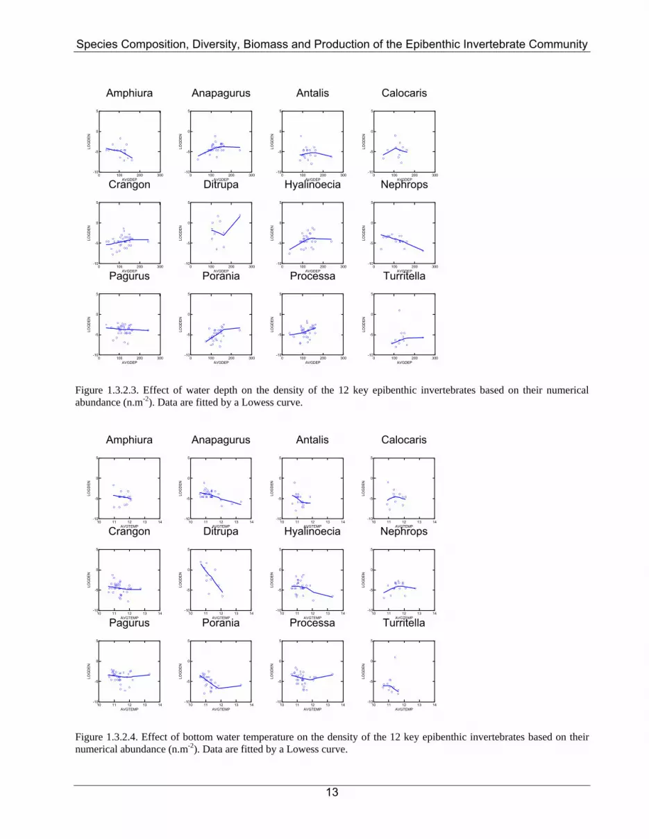
Table 1.3.1.1. Mean catching efficiency (± s.d.) of the 2-m beam trawl at the two study sites (Box A and Box N) as taken from Reiss et al. (2006). On examination of the MAFCONS 2metre beam trawl dataset it was found that the ten species covered by Reiss et al., (2006) contributed on average 17% of the total abundance and 19% of the total biomass. Although the contribution of these 10 species to the total community abundance and biomass was relatively high on average, variation, in terms of both abundance and biomass, around these means was considerable. In order to assign catching efficiencies to the entire MAFCONS species list based on the limited data available from Reiss et al., (2006), it would be necessary to make a number of major assumptions. Even if any species whose genus is represented by one or more of the 10 species covered, was assigned the raising factor of the corresponding species, most of the species in the dataset would still need to be assigned catchabilities with little or no information. Given the high variability in catching efficiencies between species within the same taxonomic group (e.g. decapods in Table 1.3.1.1.) it would be very difficult to group unrepresented species based on ‘like’ species covered in Table 1.3.1.1, particularly as the findings of Reiss et al., (2006) suggest that catchability varies based on a number of characteristics of the species including size, living position, motility and behaviour. If, however, all species whose genus was not represented were assigned a raising factor based on a mean catching efficiency, whilst those represented in Reiss et al., (2006) were assigned their species-specific raising factors, the relative contributions of species to the community (which drives species diversity and community composition analyses), would be biased by the variation in contribution of the represented species in the samples taken. However, simply raising the entire MAFCONS dataset by the catching efficiency of the entire catch (e.g. ‘All taxa’ in Table 1.3.1.1.) has its own limitations. It would provide an interesting comparison in terms of the overall difference in abundance and biomass, but would not reflect any of the changes in species diversity and community composition that result from the real variation in catchability of the different species. Because of these limitations, the effects of catchability in the 2m beam trawl on estimates of epibenthic invertebrate abundance/biomass, diversity and community composition could not be examined with the data available to the MAFCON project. Further catchability studies for 2 metre beam trawls, following the design of Reiss et al., (2006), are required so that this important issue can be properly examined in the future. 1.3.2. Abundance and distribution The majority of epibenthic taxa were relatively scarce. In total, 149,600 individual epibenthic organisms were sampled, not including the colonial taxa, and altogether 232,171g of material was processed. These epibenthic animals belonged to a total of 445 individual taxonomic classifications (species or higher level) and 13 different phyla identified over the course of the project. Of this large number of different taxa, 12 key species that dominated the epibenthic fauna on the basis of numerical abundance made up 32% of the total number of individual animals sampled, while the 12 key species that dominated the epibenthos on the basis of biomass constituted 77% of all the material processed. Spatial variation in the mean density of these key epibenthic taxa are shown in Figure 1.3.2.1 (based on numerical abundance) and Figure 1.3.2.2 (based on biomass). Variation in 2m beam trawl sampling effort between ICES rectangle had no significant impact on these abundance or biomass estimates. Each species had quite distinctive distributions, however, density was calculated, with clear regions where densities were high and, in most instances, large areas where they were either scarce or absent. At this stage only preliminary examination of the environmental factors influencing the distributions of different epibenthic taxa have been carried out. However, it is quite clear that water depth, bottom water temperature and bottom water salinity all play a role in influencing the spatial distributions of these epibenthic invertebrate with some of these factors more important than others (Figures 1.3.2.3 to 1.3.2.8).


11

53

54

55

56

57

58

59

60

Deg

rees

Lat

itude

53

54

55

56

57

58

59

60

Deg

rees

Lat

itude

53

54

55

56

57

58

59

60

Deg

rees

Lat

itude

53

54

55

56

57

58

59

60

Deg

rees

Lat

itude

-12 -10 -8 -6 -4 -2

Degrees Longitude-12 -10 -8 -6 -4 -2


Degrees Longitude

Ditrupa arietina Turritella communis

Hyalinoecia tubicola Processa canaliculata Anapagurus laevis

Crangon allmanni Nephrops norvegicus Antalis entalis

Calocaris macandreae Porania pulvillus Amphiura chiajei

Pagurus prideaux

Figure 1.3.2.1. Spatial variation in the density (nos.m-2) of the 12 most abundant epibenthic invertebrates based on abundance; Ditrupa arietina (max density 10.8), Turritella communis (max density 8.3) Pagurus prideaux (max density 0.14), Hyalinoecia tubicola (max density 0.28), Processa canaliculata (max density 0.26), Anapagurus laevis (max density 0.32), Crangon allmanni (max density 0.27), Nephrops norvegicus (max density 0.06), Antalis entails (max density 0.33), Calocaris macandreae (max density 0.36), Porania pulvillus (max density 0.09) and Amphiura chiajei (max density 0.18).


12

53

54

55

56

57

58

59

60

Deg

rees

Lat

itude

53

54

55

56

57

58

59

60

Deg

rees

Lat

itude

53

54

55

56

57

58

59

60

Deg

rees

Lat

itude

53

54

55

56

57

58

59

60

Deg

rees

Lat

itude

-12 -10 -8 -6 -4 -2



Degrees Longitude

Caryophyllia smithii Ditrupa arietina

Alcyonium digitatum Turritella communis Porania pulvillus

Pagurus prideaux Brissopsis lyrifera Nephrops norvegicus

Modiolus modiolus Adamsia carciniopados Luidia ciliaris

Actinauge richardi

Figure 1.3.2.2. Spatial variation in the density (g.m-2) of the 12 most abundant epibenthic invertebrates based on biomass; Caryphyllia smithii (max density 32.1), Ditrupa arietina (max density 9.2), Actinauge richardi (max density 2.2), Alcyonium digitatum, (max density 5.9), Turritella communis (max density 7.9), Porania pulvillus (max density 0.76), Pagurus prideaux (max density 0.63), Brissopsis lyrifera (max density 0.50), Nephrops norvegicus (max density 0.27), Modiolus modiolus (max density 3.9), Adamsia carciniopados (max density 0.20) and Luidia ciliaris (max density 0.78).


13

Amphiura

0 100 200 300AVGDEP

-10

-5

0

5

LOG

DEN

Anapagurus

0 100 200 300AVGDEP

-10

-5

0

5

LOG

DEN

Antalis

0 100 200 300AVGDEP

-10

-5

0

5

LOG

DEN

Calocaris

0 100 200 300AVGDEP

-10

-5

0

5

LOG

DEN

Crangon

0 100 200 300AVGDEP

-10

-5

0

5

LOG

DEN

Ditrupa

0 100 200 300AVGDEP

-10

-5

0

5

LOG

DEN

Hyalinoecia

0 100 200 300AVGDEP

-10

-5

0

5

LOG

DEN

Nephrops

0 100 200 300AVGDEP

-10

-5

0

5

LOG

DEN

Pagurus

0 100 200 300AVGDEP

-10

-5

0

5

LOG

DEN

Porania

0 100 200 300AVGDEP

-10

-5

0

5

LOG

DEN

Processa

0 100 200 300AVGDEP

-10

-5

0

5

LOG

DEN

Turritella

0 100 200 300AVGDEP

-10

-5

0

5

LOG

DEN

Figure 1.3.2.3. Effect of water depth on the density of the 12 key epibenthic invertebrates based on their numerical abundance (n.m-2). Data are fitted by a Lowess curve.

Amphiura

10 11 12 13 14AVGTEMP

-10

-5

0

5

LOG

DEN

Anapagurus

10 11 12 13 14AVGTEMP

-10

-5

0

5

LOG

DEN

Antalis

10 11 12 13 14AVGTEMP

-10

-5

0

5

LOG

DEN

Calocaris

10 11 12 13 14AVGTEMP

-10

-5

0

5

LOG

DE N

Crangon

10 11 12 13 14AVGTEMP

-10

-5

0

5

LOG

DEN

Ditrupa

10 11 12 13 14AVGTEMP

-10

-5

0

5

LOG

DEN

Hyalinoecia

10 11 12 13 14AVGTEMP

-10

-5

0

5

LOG

DEN

Nephrops

10 11 12 13 14AVGTEMP

-10

-5

0

5

LOG

DE N

Pagurus

10 11 12 13 14AVGTEMP

-10

-5

0

5

LOG

DEN

Porania

10 11 12 13 14AVGTEMP

-10

-5

0

5

LOG

DEN

Processa

10 11 12 13 14AVGTEMP

-10

-5

0

5

LOG

DEN

Turritella

10 11 12 13 14AVGTEMP

-10

-5

0

5

LOG

DE N

Figure 1.3.2.4. Effect of bottom water temperature on the density of the 12 key epibenthic invertebrates based on their numerical abundance (n.m-2). Data are fitted by a Lowess curve.


14

Amphiura

33 34 35 36AVGSAL

-10

-5

0

5

LOG

DEN

Anapagurus

33 34 35 36AVGSAL

-10

-5

0

5

LOG

DEN

Antalis

33 34 35 36AVGSAL

-10

-5

0

5

LOG

DEN

Calocaris

33 34 35 36AVGSAL

-10

-5

0

5

LOG

DE N

Crangon

33 34 35 36AVGSAL

-10

-5

0

5

LOG

DEN

Ditrupa

33 34 35 36AVGSAL

-10

-5

0

5

LOG

DEN

Hyalinoecia

33 34 35 36AVGSAL

-10

-5

0

5

LOG

DEN

Nephrops

33 34 35 36AVGSAL

-10

-5

0

5

LOG

DE N

Pagurus

33 34 35 36AVGSAL

-10

-5

0

5

LOG

DEN

Porania

33 34 35 36AVGSAL

-10

-5

0

5

LOG

DEN

Processa

33 34 35 36AVGSAL

-10

-5

0

5

LOG

DEN

Turritella

33 34 35 36AVGSAL

-10

-5

0

5

LOG

DE N

Figure 1.3.2.5. Effect of bottom water salinity on the density of the 12 key epibenthic invertebrates based on their numerical abundance (n.m-2). Data are fitted by a Lowess curve.

Actinauge

0 100 200 300AVGDEPTH

-10

-5

0

5

LOG

DEN

Adamsia

0 100 200 300AVGDEPTH

-10

-5

0

5

LOG

DEN

Alcyonium

0 100 200 300AVGDEPTH

-10

-5

0

5

LOG

DEN

Brissopsis

0 100 200 300AVGDEPTH

-10

-5

0

5

LOG

DEN

Caryophyllia

0 100 200 300AVGDEPTH

-10

-5

0

5

LOG

DEN

Ditrupa

0 100 200 300AVGDEPTH

-10

-5

0

5

LOG

DEN

Luidia

0 100 200 300AVGDEPTH

-10

-5

0

5

LOG

DEN

Modiolus

0 100 200 300AVGDEPTH

-10

-5

0

5

LOG

DEN

Nephrops

0 100 200 300AVGDEPTH

-10

-5

0

5

LOG

DEN

Pagurus

0 100 200 300AVGDEPTH

-10

-5

0

5

LOG

DEN

Porania

0 100 200 300AVGDEPTH

-10

-5

0

5

LOG

DEN

Turritella

0 100 200 300AVGDEPTH

-10

-5

0

5

LOG

DEN

Figure 1.3.2.6. Effect of water depth on the density of the 12 key epibenthic invertebrates based on biomass (g.m-2). Data are fitted by a Lowess curve.


15

Actinauge

10 11 12 13 14AVGTEMP

-10

-5

0

5

LOG

DEN

Adamsia

10 11 12 13 14AVGTEMP

-10

-5

0

5

LOG

DEN

Alcyonium

10 11 12 13 14AVGTEMP

-10

-5

0

5

LOG

DEN

Brissopsis

10 11 12 13 14AVGTEMP

-10

-5

0

5

LOG

DE N

Caryophyllia

10 11 12 13 14AVGTEMP

-10

-5

0

5

LOG

DEN

Ditrupa

10 11 12 13 14AVGTEMP

-10

-5

0

5

LOG

DEN

Luidia

10 11 12 13 14AVGTEMP

-10

-5

0

5

LOG

DEN

Modiolus

10 11 12 13 14AVGTEMP

-10

-5

0

5

LOG

DE N

Nephrops

10 11 12 13 14AVGTEMP

-10

-5

0

5

LOG

DEN

Pagurus

10 11 12 13 14AVGTEMP

-10

-5

0

5

LOG

DEN

Porania

10 11 12 13 14AVGTEMP

-10

-5

0

5

LOG

DEN

Turritella

10 11 12 13 14AVGTEMP

-10

-5

0

5

LOG

DE N

Figure 1.3.2.7. Effect of bottom water temperature on the density of the 12 key epibenthic invertebrates based on their biomass (g.m-2). Data are fitted by a Lowess curve.

Actinauge

33 34 35 36AVGSALINITY

-10

-5

0

5

LOG

DEN

Adamsia


-10

-5

0

5

LOG

DEN

Alcyonium


-10

-5

0

5

LOG

DEN

Brissopsis


-10

-5

0

5

LOG

DE N

Caryophyllia


-10

-5

0

5

LOG

DEN

Ditrupa


-10

-5

0

5

LOG

DEN

Luidia


-10

-5

0

5

LOG

DEN

Modiolus


-10

-5

0

5

LOG

DE N

Nephrops


-10

-5

0

5

LOG

DEN

Pagurus


-10

-5

0

5

LOG

DEN

Porania


-10

-5

0

5

LOG

DEN

Turritella


-10

-5

0

5

LOG

DE N

Figure 1.3.2.8. Effect of bottom water salinity on the density of the 12 key epibenthic invertebrates based on their biomass (g.m-2). Data are fitted by a Lowess curve.


16

1.3.3. Community species composition Group average cluster analysis of Bray-Curtis similarity matrices calculated for both the mean numerical density and mean biomass density of epibenthic invertebrates in each ICES rectangle produced the dendograms shown in Figure 1.3.3.1. Essentially the species composition of the epibenthic invertebrate community was highly variable and similarity between ICES rectangles was relatively low. Nevertheless, two main clusters were apparent for both the numerical based and biomass based density data. For convenience, all outlier rectangles were grouped together into a third small cluster. Mapping of the three clusters revealed highly contagious cluster distributions with similar spatial patterns for both the numerical and biomass density data (Figure 1.3.3.2). Furthermore, these community composition cluster maps for the epibenthic assemblage bore a marked resemblance to similar maps produced for the groundfish assemblage (Fraser & Greenstreet, 2007).


17

Abundance

36E

438

E4

41E

345

E3

44E

344

E4

43E

239

E4

39E

546

E4

45E

442

E1

42E

343

E3

38D

948

E6

39E

147

E3

45E

246

E2

47E

539

E0

42E

036

E6

46E

640

E1

41E

246

E3

40E

247

E4

41E

045

E0

42E

245

E1

46E

148

E4

41E

144

E0

43E

144

E1

39E

336

E5

46E

540

E3

Statistical Rectangle

100

80

60

40

20

0

Sim

ilarit

y

Biomass

40E

339

E3

36E

536

E6

46E

546

E6

38D

945

E2

47E

539

E1

46E

239

E0

42E

048

E6

41E

147

E3

40E

141

E0

45E

046

E3

40E

247

E4

41E

244

E0

43E

144

E1

42E

245

E1

46E

148

E4

36E

438

E4

46E

445

E4

42E

142

E3

43E

344

E3

44E

443

E2

45E

341

E3

39E

439

E5

Statistical Rectangle

100

80

60

40

20

0

Sim

ilarit

y

Figure 1.3.3.1. Group average cluster dendograms of epibenthic invertebrate density data based on mean abundance (n.m-2) and biomass (g.m-2) densities in each ICES rectangle. Colour coding links to Figure 1.3.3.2.


18

53

54

55

56

57

58

59

60

Deg

rees

Lat

itude

-12 -10 -8 -6 -4 -2

Degrees Longitude


53

54

55

56

57

58

59

60

-12 -10 -8 -6 -4 -2

Degrees Longitude

49

48

47

46

45

44

43

42

41

40

39

38

37

36

35


Abundance Biomass

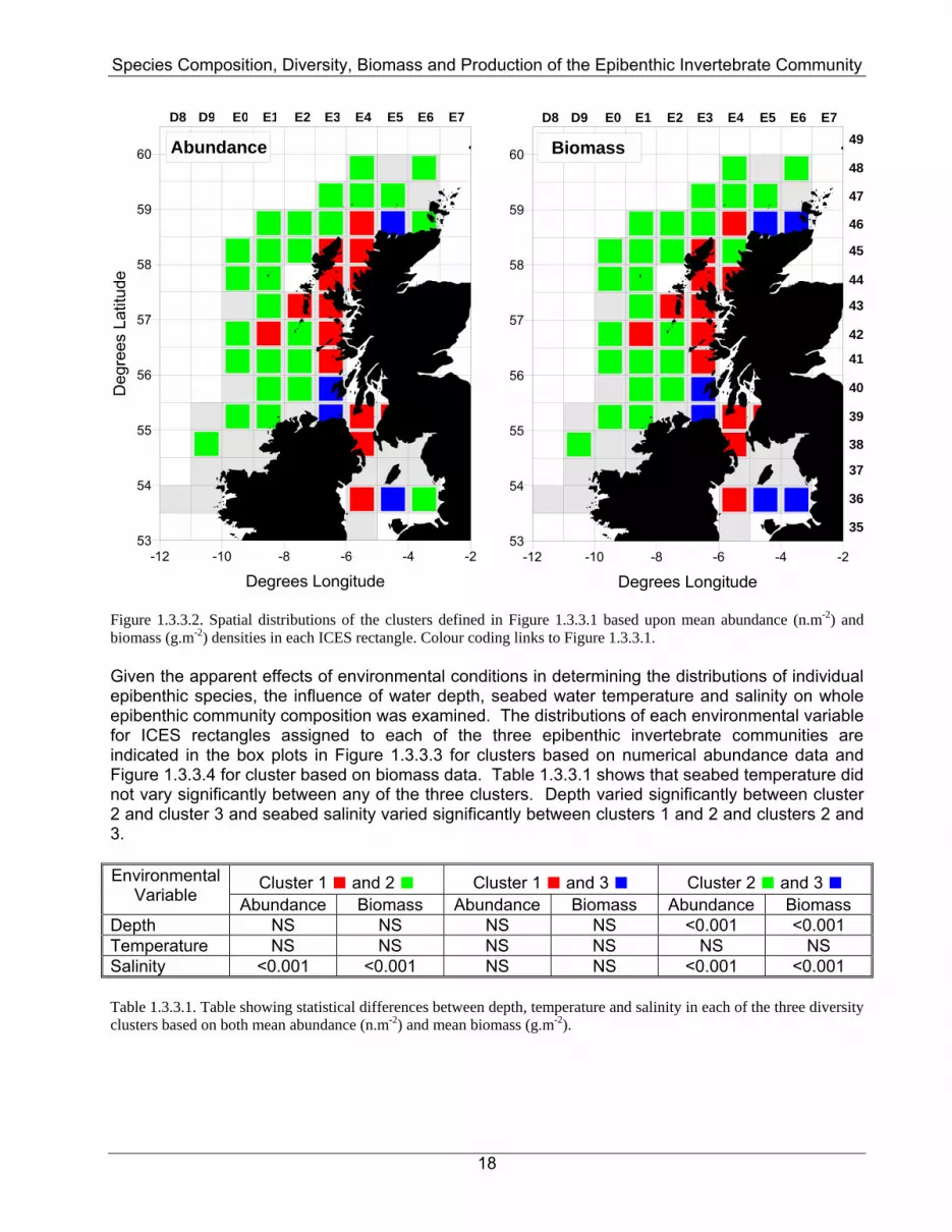
Figure 1.3.3.2. Spatial distributions of the clusters defined in Figure 1.3.3.1 based upon mean abundance (n.m-2) and biomass (g.m-2) densities in each ICES rectangle. Colour coding links to Figure 1.3.3.1. Given the apparent effects of environmental conditions in determining the distributions of individual epibenthic species, the influence of water depth, seabed water temperature and salinity on whole epibenthic community composition was examined. The distributions of each environmental variable for ICES rectangles assigned to each of the three epibenthic invertebrate communities are indicated in the box plots in Figure 1.3.3.3 for clusters based on numerical abundance data and Figure 1.3.3.4 for cluster based on biomass data. Table 1.3.3.1 shows that seabed temperature did not vary significantly between any of the three clusters. Depth varied significantly between cluster 2 and cluster 3 and seabed salinity varied significantly between clusters 1 and 2 and clusters 2 and 3.

Cluster 1 ■ and 2 ■ Cluster 1 ■ and 3 ■ Cluster 2 ■ and 3 ■ Environmental Variable Abundance Biomass Abundance Biomass Abundance Biomass

Depth NS NS NS NS <0.001 <0.001 Temperature NS NS NS NS NS NS Salinity <0.001 <0.001 NS NS <0.001 <0.001 Table 1.3.3.1. Table showing statistical differences between depth, temperature and salinity in each of the three diversity clusters based on both mean abundance (n.m-2) and mean biomass (g.m-2).


19

0.5 1.0 1.5 2.0 2.5 3.0 3.5CLUSTER

0

100

200

300A

VG

DE

PTH

0.5 1.0 1.5 2.0 2.5 3.0 3.5CLUSTER

10

11

12

13

14

AV

GTE

MP

0.5 1.0 1.5 2.0 2.5 3.0 3.5CLUSTER

33

34

35

36

AV

GS

ALI

NIT

Y

Figure 1.3.3.3. Box plots showing the range in water depth, bottom temperature and bottom salinity associated with each epibenthic community type cluster based on numerical abundance identified in Figures 1.3.3.1 and 1.3.3.2.

0.5 1.0 1.5 2.0 2.5 3.0 3.5CLUSTER

0

100

200

300

AV

GD

EP

TH

0.5 1.0 1.5 2.0 2.5 3.0 3.5CLUSTER

10

11

12

13

14

AV

GTE

MP

0.5 1.0 1.5 2.0 2.5 3.0 3.5CLUSTER

33

34

35

36

AV

GS

ALI

NIT

Y

Figure 1.3.3.4. Box plots showing the range in water depth, bottom temperature and bottom salinity associated with each epibenthic community type cluster based on biomass identified in Figures 1.3.3.1 and 1.3.3.2.


20

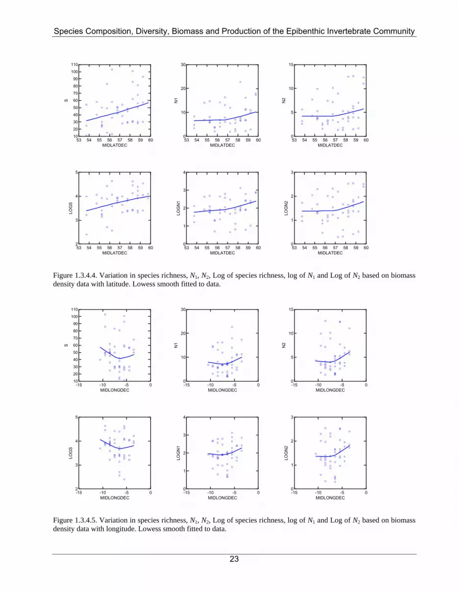
1.3.4. Community species richness and species diversity Epibenthic species richness and species diversity varied markedly between ICES rectangles with no real trends apparent (Figure 1.3.4.1). Plots of species richness and Hill’s N1 and N2, based on either numerical abundance or biomass, against both latitude and longitude confirmed the lack of trends (Figures 1.3.4.2 to 1.3.4.5). Table 1.3.4.1 and Figures 1.3.4.6 and 1.3.4.7 show that there was no significant difference between Hill’s N1 and N2 in any of the three clusters. There was however a significant difference between species richness (S) in clusters 1 and 2. The effects of water depth, bottom water temperature and salinity are shown in Figures 1.3.4.8 to 1.3.4.10 for metrics based on numerical abundance and in Figures 1.3.4.11 to 1.3.4.13 for metrics based on biomass. Effects of water depth and bottom water temperature and salinity are suggested, but in each case the relationships are curvilinear or unimodal.

Cluster 1 ■ and 2 ■ Cluster 1 ■ and 3 ■ Cluster 2 ■ and 3 ■ Diversity Index Abundance Biomass Abundance Biomass Abundance Biomass

S NS <0.001 NS NS NS NS N1 NS NS NS NS NS NS N2 NS NS NS NS NS NS Table 1.3.4.1. Table showing statistical differences between S, N1 and N2 in each of the three diversity clusters based on both mean abundance (n.m-2) and mean biomass (g.m-2).


21

53

54

55

56

57

58

59

60

Deg

rees

Lat

itude

-12 -10 -8 -6 -4 -2

Degrees Longitude

49

48

47

46

45

44

43

42

41

40

39

38

37

36

35

E7E6E5E4E3E2E1E0D9D8 10 to 20 20 to 30 30 to 40 40 to 50 50 to 60 60 to 70 70 to 80 80 to 90 90 to 100 100 to 110

-12 -10 -8 -6 -4 -2

Degrees Longitude

E7E6E5E4E3E2E1E0D9D8 0 to 2 2 to 4 4 to 6 6 to 8

8 to 10 10 to 15 15 to 20 20 to 25

-12 -10 -8 -6 -4 -2

Degrees Longitude

E7E6E5E4E3E2E1E0D9D8 0 to 2 2 to 4 4 to 6 6 to 8 8 to 10 10 to 15

S N1 N2

Biomass

53

54

55

56

57

58

59

60

Deg

rees

Lat

itude

-12 -10 -8 -6 -4 -2

Degrees Longitude

49

48

47

46

45

44

43

42

41

40

39

38

37

36

35

E7E6E5E4E3E2E1E0D9D8 5 to 10 10 to 20 20 to 30 30 to 40 40 to 50 50 to 60 60 to 70 70 to 80 80 to 90 90 to 100

-12 -10 -8 -6 -4 -2

Degrees Longitude

E7E6E5E4E3E2E1E0D9D8 0 to 2 2 to 4 4 to 6 6 to 8 8 to 10 10 to 15 15 to 20 20 to 25 25 to 30 30 to 35 35 to 40 40 to 50 50 to 60

-12 -10 -8 -6 -4 -2

Degrees Longitude

E7E6E5E4E3E2E1E0D9D8 0 to 2 2 to 4

4 to 6 6 to 8 8 to 10 10 to 15 15 to 20 20 to 25 25 to 30 30 to 35 35 to 40 40 to 50

S N1 N2

Abundance

Figure 1.3.4.1. Spatial variation in species richness (S) and Hills N1 and N2 calculated on mean sample abundance and biomass data in each ICES statistical rectangle.


22

53 54 55 56 57 58 59 60MIDLATDEC

0

10

20

30

40

50

60

70

80

90

100S

53 54 55 56 57 58 59 60MIDLATDEC

0

10

20

30

40

50

60

N1

53 54 55 56 57 58 59 60MIDLATDEC

0

10

20

30

40

50

N2

53 54 55 56 57 58 59 60MIDLATDEC

2

3

4

5

LOG

S

53 54 55 56 57 58 59 60MIDLATDEC

0

1

2

3

4

5LO

GN

1

53 54 55 56 57 58 59 60MIDLATDEC

0

1

2

3

4

LOG

N2

Figure 1.3.4.2. Variation in species richness, N1, N2, Log of species richness, log of N1 and Log of N2 based on numerical density data with latitude. Lowess smooth fitted to data.

-15 -10 -5 0MIDLONGDEC

0

10

20

30

40

50

60

70

80

90

100

S


0

10

20

30

40

50

60

N1


0

10

20

30

40

50

N2


2

3

4

5

LOG

S


0

1

2

3

4

5

LOG

N1


0

1

2

3

4

LOG

N2

Figure 1.3.4.3. Variation in species richness, N1, N2, Log of species richness, log of N1 and Log of N2 based on numerical density data with longitude. Lowess smooth fitted to data.


23

53 54 55 56 57 58 59 60MIDLATDEC

10

20

30

40

50

60

70

80

90

100

110S

53 54 55 56 57 58 59 60MIDLATDEC

0

10

20

30

N1

53 54 55 56 57 58 59 60MIDLATDEC

0

5

10

15

N2

53 54 55 56 57 58 59 60MIDLATDEC

2

3

4

5

LOG

S

53 54 55 56 57 58 59 60MIDLATDEC

0

1

2

3

4LO

GN

1

53 54 55 56 57 58 59 60MIDLATDEC

0

1

2

3

LOG

N2

Figure 1.3.4.4. Variation in species richness, N1, N2, Log of species richness, log of N1 and Log of N2 based on biomass density data with latitude. Lowess smooth fitted to data.


10

20

30

40

50

60

70

80

90

100

110

S


0

10

20

30

N1


0

5

10

15

N2


2

3

4

5

LOG

S


0

1

2

3

4

LOG

N1


0

1

2

3

LOG

N2

Figure 1.3.4.5. Variation in species richness, N1, N2, Log of species richness, log of N1 and Log of N2 based on biomass density data with longitude. Lowess smooth fitted to data.


24

0.5 1.0 1.5 2.0 2.5 3.0 3.5ABUNDANCE

0

10

20

30

40

50

60

70

80

90

100S

0.5 1.0 1.5 2.0 2.5 3.0 3.5ABUNDANCE

0

10

20

30

40

50

60

N1

0.5 1.0 1.5 2.0 2.5 3.0 3.5ABUNDANCE

0

10

20

30

40

50

N2

0.5 1.0 1.5 2.0 2.5 3.0 3.5ABUNDANCE

2

3

4

5

LOG

S

0.5 1.0 1.5 2.0 2.5 3.0 3.5ABUNDANCE

0

1

2

3

4

5LO

GN

1

0.5 1.0 1.5 2.0 2.5 3.0 3.5ABUNDANCE

0

1

2

3

4

LOG

N2

Figure 1.3.4.6. Box plots showing the range in species richness, N1, N2, Log of species richness, log of N1 and Log of N2 associated with each epibenthic community type cluster based on numerical abundance identified in Figures 1.3.3.1 and 1.3.3.2.

0.5 1.0 1.5 2.0 2.5 3.0 3.5BIOMASS

10

20

30

40

50

60

70

80

90

100

110

S

0.5 1.0 1.5 2.0 2.5 3.0 3.5BIOMASS

0

10

20

30

N1

0.5 1.0 1.5 2.0 2.5 3.0 3.5BIOMASS

0

5

10

15

N2

0.5 1.0 1.5 2.0 2.5 3.0 3.5BIOMASS

2

3

4

5

LOG

S

0.5 1.0 1.5 2.0 2.5 3.0 3.5BIOMASS

0

1

2

3

4

LOG

N1

0.5 1.0 1.5 2.0 2.5 3.0 3.5BIOMASS

0

1

2

3

LOG

N2

Figure 1.3.4.7. Box plots showing the range in species richness, N1, N2, Log of species richness, log of N1 and Log of N2 associated with each epibenthic community type cluster based on biomass identified in Figures 1.3.3.1 and 1.3.3.2.


25

0 100 200 300AVGDEPTH

0

10

20

30

40

50

60

70

80

90

100S

0 100 200 300AVGDEPTH

0

10

20

30

40

50

60

N1

0 100 200 300AVGDEPTH

0

10

20

30

40

50

N2

0 100 200 300AVGDEPTH

2

3

4

5

LOG

S

0 100 200 300AVGDEPTH

0

1

2

3

4

5LO

GN

1

0 100 200 300AVGDEPTH

0

1

2

3

4

LOG

N2

Figure 1.4.3.8. Relationships between species richness, N1, N2, Log of species richness, log of N1 and Log of N2 based on numerical abundance and water depth. Data fitted with a Lowess smoother.

10 11 12 13 14AVGTEMP

0

10

20

30

40

50

60

70

80

90

100

S

10 11 12 13 14AVGTEMP

0

10

20

30

40

50

60

N1

10 11 12 13 14AVGTEMP

0

10

20

30

40

50

N2

10 11 12 13 14AVGTEMP

2

3

4

5

LOG

S

10 11 12 13 14AVGTEMP

0

1

2

3

4

5

LOG

N1

10 11 12 13 14AVGTEMP

0

1

2

3

4

LOG

N2

Figure 1.4.3.9. Relationships between species richness, N1, N2, Log of species richness, log of N1 and Log of N2 based on numerical abundance and bottom water temperature. Data fitted with a Lowess smoother.


26


0

10

20

30

40

50

60

70

80

90

100S


0

10

20

30

40

50

60

N1


0

10

20

30

40

50

N2


2

3

4

5

LOG

S


0

1

2

3

4

5LO

GN

1


0

1

2

3

4

LOG

N2

Figure 1.4.3.10. Relationships between species richness, N1, N2, Log of species richness, log of N1 and Log of N2 based on numerical abundance and bottom water salinity. Data fitted with a Lowess smoother.

0 100 200 300AVGDEPTH

10

20

30

40

50

60

70

80

90

100

110

S

0 100 200 300AVGDEPTH

0

10

20

30

N1

0 100 200 300AVGDEPTH

0

5

10

15

N2

0 100 200 300AVGDEPTH

2

3

4

5

LOG

S

0 100 200 300AVGDEPTH

0

1

2

3

4

LOG

N1

0 100 200 300AVGDEPTH

0

1

2

3

LOG

N2

Figure 1.4.3.11. Relationships between species richness, N1, N2, Log of species richness, log of N1 and Log of N2 based on biomass and water depth. Data fitted with a Lowess smoother.


27

10 11 12 13 14AVGTEMP

10

20

30

40

50

60

70

80

90

100

110S

10 11 12 13 14AVGTEMP

0

10

20

30

N1

10 11 12 13 14AVGTEMP

0

5

10

15

N2

10 11 12 13 14AVGTEMP

2

3

4

5

LOG

S

10 11 12 13 14AVGTEMP

0

1

2

3

4LO

GN

1

10 11 12 13 14AVGTEMP

0

1

2

3

LOG

N2

Figure 1.4.3.12. Relationships between species richness, N1, N2, Log of species richness, log of N1 and Log of N2 based on biomass and bottom water temperature. Data fitted with a Lowess smoother.


10

20

30

40

50

60

70

80

90

100

110

S


0

10

20

30

N1


0

5

10

15

N2


2

3

4

5

LOG

S


0

1

2

3

4

LOG

N1


0

1

2

3

LOG

N2

Figure 1.4.3.13. Relationships between species richness, N1, N2, Log of species richness, log of N1 and Log of N2 based on biomass and bottom water salinity. Data fitted with a Lowess smoother.


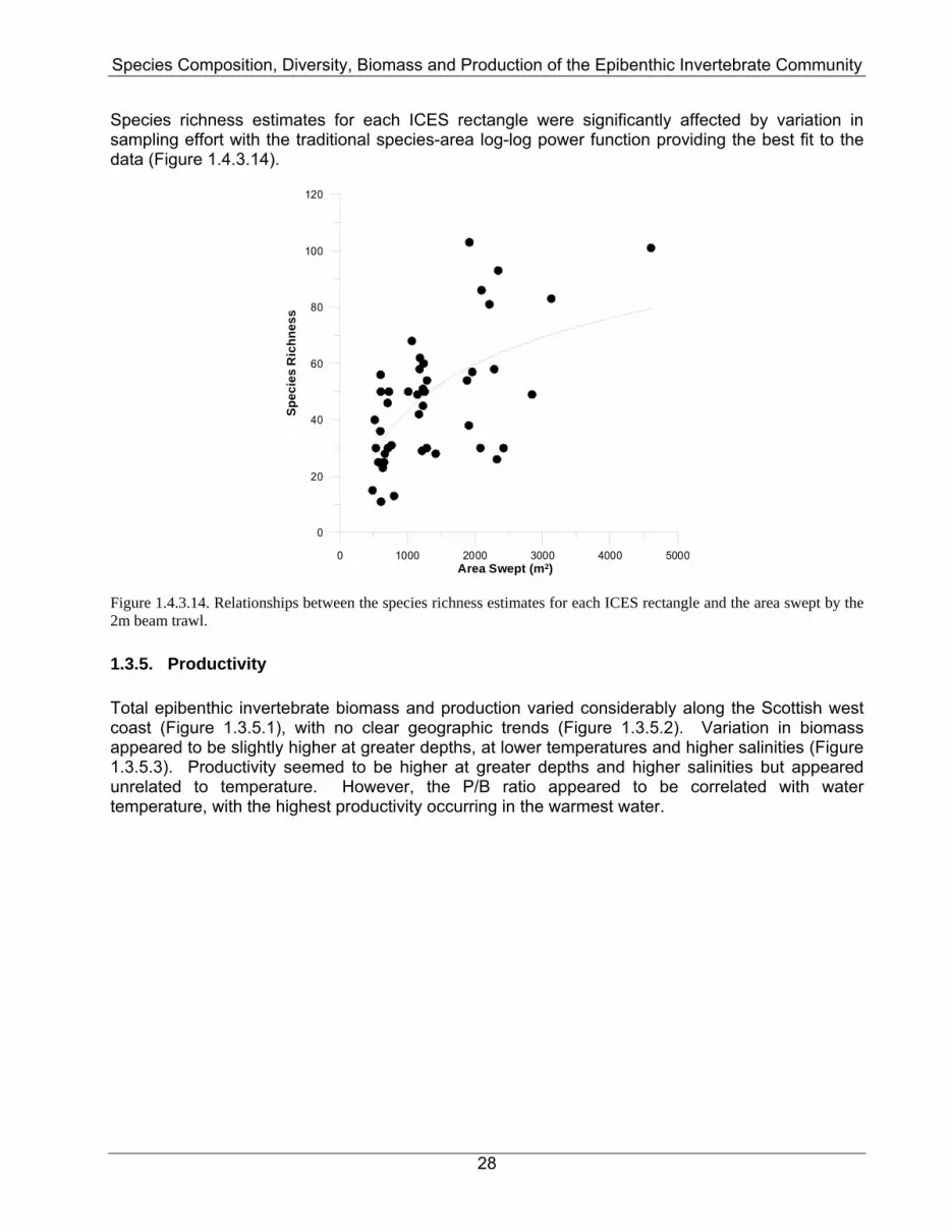
28

Species richness estimates for each ICES rectangle were significantly affected by variation in sampling effort with the traditional species-area log-log power function providing the best fit to the data (Figure 1.4.3.14).

0 1000 2000 3000 4000 5000Area Swept (m2)

0

20

40

60

80

100

120

Spec

ies

Ric

hnes

s

Figure 1.4.3.14. Relationships between the species richness estimates for each ICES rectangle and the area swept by the 2m beam trawl. 1.3.5. Productivity Total epibenthic invertebrate biomass and production varied considerably along the Scottish west coast (Figure 1.3.5.1), with no clear geographic trends (Figure 1.3.5.2). Variation in biomass appeared to be slightly higher at greater depths, at lower temperatures and higher salinities (Figure 1.3.5.3). Productivity seemed to be higher at greater depths and higher salinities but appeared unrelated to temperature. However, the P/B ratio appeared to be correlated with water temperature, with the highest productivity occurring in the warmest water.


29

53

54

55

56

57

58

59

60

Deg

rees

Lat

itude

-12 -10 -8 -6 -4 -2

Degrees Longitude

49

48

47

46

45

44

43

42

41

40

39

38

37

36

35

E7E6E5E4E3E2E1E0D9D8 0.0 to 0.5 0.5 to 1.0 1.0 to 1.5 1.5 to 2.0 2.0 to 2.5 2.5 to 5.0 5.0 to 7.5 7.5 to 10.0 10.0 to 15.0 15.0 to 20.0 20.0 to 25.0 25.0 to 30.0

-12 -10 -8 -6 -4 -2

Degrees Longitude

E7E6E5E4E3E2E1E0D9D8 0 to 10 10 to 20 20 to 30 30 to 40 40 to 50 50 to 60 60 to 70 70 to 80 80 to 90 90 to 100 100 to 200 200 to 400 400 to 900

-12 -10 -8 -6 -4 -2

Degrees Longitude

E7E6E5E4E3E2E1E0D9D8 0.00 to 0.02 0.02 to 0.04 0.04 to 0.06 0.06 to 0.08 0.08 to 0.10 0.10 to 0.12 0.12 to 0.14 0.14 to 0.16 0.16 to 0.18 0.18 to 0.20 0.20 to 0.30

B P P/B

Figure 1.3.5.1. Plots of the spatial distribution of total epibenthic invertebrate biomass (g.m-2) (B), secondary production (mg.m-2.d-1) (P), and the production/biomass ratio (P/B).

53 54 55 56 57 58 59 60MIDLATDEC

-3

-2

-1

0

1

2

3

4

LOG

BIO

MA

SS

53 54 55 56 57 58 59 60MIDLATDEC

1

2

3

4

5

6

7

LOG

DAI

LYPR

OD

53 54 55 56 57 58 59 60MIDLATDEC

0.0

0.1

0.2

0.3

PB


-3

-2

-1

0

1

2

3

4

LOG

BI O

MA

SS


1

2

3

4

5

6

7

LOG

DAI

LYP R

OD


0.0

0.1

0.2

0.3

PB

Figure 1.3.5.2. Relationships between Log biomass (B) (g.m-2), Log production (P) (mg.m-2.d-1) and the production-biomass ratio (PB) and latitude and longitude. Data fitted with a Lowess smoother.


30

0 100 200 300AVGDEPTH

-3

-2

-1

0

1

2

3

4LO

GB

I OM

AS

S

0 100 200 300AVGDEPTH

1

2

3

4

5

6

7

LOG

DAI

L YPR

OD

0 100 200 300AVGDEPTH

0.0

0.1

0.2

0.3

PB

10 11 12 13 14AVGTEMP

-3

-2

-1

0

1

2

3

4

LOG

B IO

MAS

S

10 11 12 13 14AVGTEMP

1

2

3

4

5

6

7

LOG

DA

ILYP

RO

D

10 11 12 13 14AVGTEMP

0.0

0.1

0.2

0.3

PB


-3

-2

-1

0

1

2

3

4

LOG

BIO

MA

SS


1

2

3

4

5

6

7

LOG

DAI

LYPR

OD


0.0

0.1

0.2

0.3

PB

Figure 1.3.5.3. Relationships between Log biomass (B) (g.m-2), Log production (P) (mg.m-2.d-1) and the production-biomass ratio (PB) and water depth (m) and bottom water temperature (ºC) and salinity. Data fitted with a Lowess smoother. The relationships between species richness and diversity and biomass, productivity and productivity-biomass ratios were examined (Figure 1.3.5.4). Species richness was positively related with both biomass and productivity. However, such relationships are common and are invariably due to the increased probability of sampling rarer species when abundance/biomass is higher generally (Gaston & Matter 2002). More interestingly though, there was no relationship between P/B ratio and species richness. Productivity was negatively related to both Hill’s N1 and Hill’s N2 (R=-0.17, P<0.05 and R=-0.22, <0.05 respectively). There was no relationship between the P/B ratio and Hill’s N1 and Hill’s N2. These relationships run contra to current general dogma, that increased biodiversity leads to raised productivity (Emmerson & Huxham 2002; Tilman et al., 2001; 2002; Worm & Duffy 2003).


31

2 3 4 5LOG_S

-3

-2

-1

0

1

2

3

4LO

GB

I OM

AS

S

2 3 4 5LOG_S

1

2

3

4

5

6

7

LOG

DAI

LYP R

OD

2 3 4 5LOG_S

0.0

0.1

0.2

0.3

PB

0 1 2 3 4 5LOG_N1

-3

-2

-1

0

1

2

3

4

LOG

BIO

MAS

S

0 1 2 3 4 5LOG_N1

1

2

3

4

5

6

7

LOG

DA

ILYP

RO

D

0 1 2 3 4 5LOG_N1

0.0

0.1

0.2

0.3

PB

0 1 2 3 4LOG_N2

-3

-2

-1

0

1

2

3

4

LOG

BI O

MA

SS

0 1 2 3 4LOG_N2

1

2

3

4

5

6

7

LOG

DAI

LYP R

OD

0 1 2 3 4LOG_N2

0.0

0.1

0.2

0.3

PB

Figure 1.3.5.4. Relationships between Log biomass (B) (g.m-2), Log production (P) (mg.m-2.d-1) and the species richness and diversity of the epibenthic invertebrate community. Data fitted with a Lowess smoother. 1.3.6. Fish caught in the 2m beam trawl The 2m beam trawl is not designed to catch fish but as demersal fish are associated with the seabed they are invariably caught in the epibenthic samples. In total over the four years sampled, 49 different species of fish were caught in the 2m beam trawl off the Scottish west coast ranging from a lesser spotted dogfish (Scyliorhinus canicula) at 75cm to a spotted dragonet (Callionymus maculatus) at 1.6cm. Most of the fish species caught in the 2m beam trawl are small animals, mainly juvenile flatfish such as long rough dab (Hippoglossoides platessoides), small species of flatfish such as scaldfish (Arnoglossus laterna) and thickback sole (Microchirus variegatus), gobies (Pomatoschistus minutus, Lesueurigobius friesii) and small dragonets (Callionymus maculatus, Callionymus lyra). Figure 1.3.6.1 shows the density and distribution of the top 12 fish species by number.


32

53

54

55

56

57

58

59

60

Deg

rees

Lat

itude

53

54

55

56

57

58

59

60

Deg

rees

Lat

itude

53

54

55

56

57

58

59

60

Deg

rees

Lat

itude

53

54

55

56

57

58

59

60

Deg

rees

Lat

itude

-12 -10 -8 -6 -4 -2



Degrees Longitude

Pomatoschistus minutus Gadiculus argenteus

Lepidorhombus whiffiagonis Callionymus lyra Trisopterus minutus

Lesueurigobius friesii Callionymus maculatus Glyptocephalus cynoglossus

Microchirus variegatus Ammodytes marinus Arnoglossus laterna

Trisopterus esmarkii

Figure 1.3.6.1. Spatial variation in the density (g.m-2) of the 12 most abundant fish species based on abundance caught in the 2m beam trawl; Pomatoschistus minutus – sand goby (max density 0.14), Gadiculus argenteus – silvery pout (max density 0.03), Trisopterus esmarkii – Norway pout (max density 0.02), Lepidorhombus whiffiagonis - megrim, (max density 0.01), Callionymus lyra - dragonet (max density 0.01), Trisopterus minutus – poor cod (max density 0.008), Lesueurigobius friesii – Fries goby (max density 0.03), Callionymus maculatus – spotted dragonet (max density 0.007), Glyptocephalus cynoglossus - witch (max density 0.02), Microchirus variegates – thickback sole (max density 0.007), Ammodytes marinus – Raitt’s sandeel (max density 0.4) and Arnoglossus laterna - scaldfish (max density 0.01).


33

1.4. DISCUSSION AND CONCLUSIONS The majority of epibenthic taxa off the Scottish west coast were relatively scarce. The epibenthic animals belonged to 445 individual taxonomic classifications and 13 different phyla. The 12 most abundant invertebrate species based on abundance accounted for 32% of the total number of individuals sampled. The mollusc Ditrupa arietina was the most abundant animal based on numbers. The most abundant animal based on biomass was the Devonshire Cup Coral (Caryophyllia smithii; Cnidaria). Looking at the relationship between density and three environmental variables (depth, temperature and salinity), there were few significant relationships. The only significant relationship was a strong negative correlation between the density of Ditrupa arietina and temperature. Analysis of the community composition showed two main community clusters. Analysis showed no difference in temperature between the three clusters, but there were some significant differences in depth and salinity. Epibenthic species richness and species diversity varied markedly between ICES rectangles with no real trends apparent. Species richness was highest in 41E0 both in terms of abundance and biomass and 36E4 was the lowest both in terms of abundance and biomass. Hill’s N1 was highest in 45E4 (in terms of both abundance and biomass) indicating that no one species dominates the community. There was no variation in species richness or diversity with latitude, longitude, depth, temperature or salinity. Total epibenthic invertebrate biomass and production varied considerably along the Scottish west coast with no clear geographic trends. Variation in biomass appeared to be slightly higher at greater depths, at lower temperatures and higher salinities. Productivity seemed to be higher at greater depths and higher salinities. P/B ration appeared to be correlated with water temperature, with the highest productivity occurring in the warmest water. Most fish species caught in the 2m beam trawl were small animals mainly juvenile flatfish, small bodied flatfish such as scaldfish and thickback sole and small fish such as dragonets and gobies.


34

1.5. REFERENCES Banse, K. & Mosher, S. (1980) Adult body mass and annual production/biomass relationships of field populations. Ecological Monographs, 50, 355-359. Basford, D. J., Eleftheriou, A. & Rafaelli, D. (1989) The epifauna of the northern North Sea (56-61°N). Journal of the Marine Biological Association UK, 69, 387-407. Brey, T. (1999) A collection of empirical relations for use in ecological modelling. NAGA The ICLARM Quarterly, 22, 24-28. Brey, T. (1990) Estimating productivity of macrobenthic invertebrates from biomass and mean individual weight. Meeresforsch, 32, 329-343. Brey, T. (2002) Population Dynamics in Benthic Invertebrates A Virtual Handbook. 2002. Brey, T., Jarre-Teichmann, A. & Borlich, O. (1996) Artificial neural network versus multiple linear regression: Predicting P/B ratios from empirical data. Marine Ecology Progress Series, 140, 251-256. Callaway, R., Alsvag, J., de Boois, I., Cotter, J., Ford, A., Hinz, H., Jennings, S., Kröncke, I., Lancaster, J., Piet, G., Prince, P. & Ehrich, S. (2002) Diversity and community structure of epibenthic invertebrates and fish in the North Sea. ICES Journal of Marine Science, 59, 1199-1214. Clarke, K. R. & Warwick, R. M. (2001) Change in Marine Communities: an Approach to Statistical Analysis and Interpretation. 2nd Edition. PRIMER-E, Plymouth, UK. Colwell, R. K. & Coddington, J. A. (1994) Estimating terrestrial biodiversity through extraplolation. Philosophical Transactions of the Royal Society of London, Series B, 345, 101-118. Connor, E. F., Courtney, A. C. & Yoder, J. M. (2000) Individuals-area relationships: the relationship between animal population density and area. Ecology, 81, 734-748. Crisp, D. J. (1984) Energy flow measurements. (eds N. A. Holme & A. D. McIntyre). Cushman, R. M., Shugart, H. H. Jr., Hildebrand, S. G. & Elwood, J. W. (1978) The effect of growth curve and sampling regime on instantaneous-growth, removal-summation, and Hynes/Hamilton estimates of aquatic insect production: A computer simulation. Limnology and Oceanography, 23, 184-189. Edgar, G. J. (1990a) The influence of plant structure on the species richness, biomass and secondary production of macrofaunal essemblages associated with Western Australian seagrass beds. Journal of Experimental Marine Biology and Ecology, 137, 215-240. Edgar, G. J. (1990b) The use of the size structure of benthic macro-faunal communities to estimate faunal biomass and secondary production. Journal of Experimental Marine Biology and Ecology, 137, 195-214. Eleftheriou, A. & Basford, D. J. (1989) The macrobenthic infauna of the offshore northern North Sea. Journal of the Marine Biological Association of the United Kingdom, 69, 123-143.


35

Ellis, J. R., Rogers, S. I. & Freeman, S. M (2000) Demersal assemblages in the Irish Sea, St George’s Channel and Bristol Channel. Estuarine, Coastal and Shelf Science, 51, 299-315. Emmerson, M. & Huxham, M. (2002) How can marine ecology contribute to the biodiversity-ecosystem functioning debate? Biodiversity and Ecosystem Functioning: Synthesis and Perspectives (eds M. Loreau, S. Naeem & P. Inchausti), pp. 139-146. Oxford University Press, Oxford, UK. Fraser, H. M. & Greenstreet, S. P. R. (2007) Species composition, diversity and biomass of the demersal fish community off the Scottish west coast. FRS Internal Report. Frauenheim, K., Neumann, V., Thiel, H. & Tuerkay, M. (1989) The distribution of larger epifauna during summer and winter in the North Sea and its suitability for environmental monitoring. Senkenbergiana maritima, 20, 101-118. Gaston, K. J. & Matter, S. F. (2002) Individuals-area relationships: comment. Ecology, 83, 288-293. Gotelli, N. J. & Colwell, R. K. (2001) Quantifying biodiversity: procedures and pitfalls in the measurement and comparison of species richness. Ecology Letters, 4, 379-391. Hayward, P. J. & Ryland, J. S. (1990) The Marine fauna of the British Isles and North-West Europe. Clarendon Press, Oxford. Heip, C., Huys, R. & Alkemade, R. (1992) Community structure and functional roles of meiofauna in the North Sea. Netherlands Journal of Aquatic Ecology, 26. Hensley, R. H. (1996) Preliminary survey of benthos from the Nephrops norvegicus mud grounds in the north-western Irish Sea. Estuarine, Coastal and Shelf Science, 42, 457-465. Howson, C. M. & Picton, B. E. The Species Directory of the Marine Faune and Flora of the British Isles and Surrounding Seas. Ulster Museum and the Marine Conservation Society, Belfast and Ross-on-Wye. Jennings, S., Dinmore, T. A., Duplisea, D. E. & Lancaster, J. E. (2001) Trawling disturbance can modify benthic production processes. Journal of Animal Ecology, 70. Jennings, S., Lancaster, J., Woolmer, A. & Cotter, J. (1999) Distribution, diversity and abundance of epibenthic fauna in the North Sea. Journal of the Marine Biological Association of the United Kingdom, 79, 385-399. Magurran, A. E. (1988) Ecological Diversity and Its Measurement. Chapman and Hall, London. Morin, A. & Bourassa, N. (1992) Empirical models of the annual production and P/B (productivity/biomass) of benthic invertebrates in running water. Canadian Journal of Fisheries and Aquatic Sciences, 49, 532-539. Morin, A., Mousseau, T. A. & Roff, D. A. (1987) Accuracy and precision of secondary production estimates. Limnology and Oceanography, 32, 1342-1352. Pinn, E. H. & Robertson, M. R. (2003) Macro-faunal biodiversity and analysis of associated feeding guilds in the Greater Minch area, Scottish west coast. Journal of the Marine Biological Association of the United Kingdom, 83, 433-443.


36

Plante, C. & Downing, J. A. (1989) Production of freshwater invertebrate populations in lakes. Canadian Journal of Fisheries and Aquatic Sciences., 46, 1489-1498. Reiss, H., Kroncke, I. & Ehrich, S. (2006) Estimating the catching efficiency of a 2-m beam trawl for sampling epifauna by removal experiments. ICES Journal of Marine Science, 63, 1453-1464. Robertson, A. I. (1979) The relationship between annual production: biomass ratios and lifespans for marine macrobenthos. Oecologia, 38, 193-202. Schwinghamer, P., Hargrave, B., Peer, D. & Hawkins, C. M. (1986) Partitioning of production and respiration among size groups of organisms in an intertidal benthic community. Marine Ecology Progress Series, 31, 131-142. Southwood, T. R. E. (1978) Ecological Methods: with Particular Reference to the Study of Insect Populations. Chapman and Hall, London. Swift, D. J. (1993) The macrobenthic infauna off Sellafield (north-eastern Irish Sea) with special reference to bioturbation. Journal of the Marine Biological Association of the United Kingdom, 73, 143-162. Tilman, D., Knops, J., Wedin, D. & Reich. P. (2001) Experimental and observational studies of diversity, productivity and stability. Functional Consequences of Biodiversity: Experimental Progress and Theoretical Extensions (eds A. P. S. Kinzig & D. Tilman), pp. 42-70. Princton University Press, New Jersey, U.S.A. Tilman, D., Knops, J., Wedin, D. & Reich, P. (2002) Plant diversity and composition: effects on productivity and nutrient dynamics of experimental grasslands. Biodiversity and Ecosystem Functioning: Synthesis and Perspectives (eds M. Loreau, S. Naeem & P. Inchausti), pp. 21-35. Oxford University Press, Oxford, UK. Tumbiolo, M. L. & Downing, J. A. (1994) An empirical model for the prediction of secondary production in marine benthic invertebrate populations. Marine Ecology Progress Series, 114, 165-174. van Gemerden, B. S., Etienne, R. S., Olff, H., Hommel, P. W. F. M. & van Langevelde, F. (2005) Reconciling methodologically different biodiversity assessments. Ecological Applications, 15, 1747-1760. Wildish, D. J. & Peer, D. (1981) Methods for Estimating Secondary Production in Marine Amphipoda. Canadian Journal of Fisheries and Aquatic Sciences, 38, 1019-1026. Worm, B. & Duffy, J. E. (2003) Biodiversity, productivity and stability in real food webs. TRENDS in Ecology and Evolution, 18 , 628-632. Zühlke, R., Alsvĺg, J., de Boois, I., Cotter, J., Ford, A., Hinz, H., Jarre-Teichmann, A., Jennings, S., Kröncke, I., Lancaster, J., Piet, G. & Prince, P. (2001) Epibenthic diversity in the North Sea. Burning Issues of North Sea Ecology (eds I. Kröncke, M. Türkay & J. Sunderman), pp. 99-372.

Date post:	25-Nov-2023
Category:	Documents
Upload:	swansea
View:	0 times
Download:	0 times

Species composition, diversity, biomass and production of the benthic invertebrate community of the...

Documents