MATHEMATICS OF COMPUTATIONVOLUME 38, NUMBER 158APRIL 1982, PAGES 517-529
The Numerical Evaluation of Very OscillatoryInfinite Integrals by Extrapolation
By Avram Sidi
Abstract. Recently the author has given two modifications of a nonlinear extrapolationmethod due to Levin and Sidi, which enable one to accurately and economically computecertain infinite integrals whose integrands have a simple oscillatory behavior at infinity. Inthis work these modifications are extended to cover the case of very oscillatory infiniteintegrals whose integrands have a complicated and increasingly rapid oscillatory behavior atinfinity. The new method is applied to a number of complicated integrals, among them thesolution to a problem in viscoelasticity. Some convergence results for this method arepresented.
1. Introduction. Recently Levin and Sidi [4] have given some nonlinear transfor-mations for accelerating the convergence of slowly converging infinite integrals andseries, namely the D- and ¿-transformations, respectively, which have proved to bevery efficient numerically. Convergence properties of these transformations, whichare generalizations of the Richardson extrapolation process, have been analyzed in aseries of papers by the present author, and some results, which, to a certain extent,explain how these transformations work, have been given, see Sidi [9], [10], [11].Actually, Sidi [9], [11] deal specifically with the case of the T-transformation ofLevin [2], which is a special case of the ¿-transformation, and Sidi [10] deals with thegeneralized Richardson extrapolation process, which has as special cases the D- and¿-transformations.
Two useful modifications of the ^-transformation (the D- and ¿-transformations)that simplify the computation of oscillatory infinite integrals, with special emphasison Fourier and Hankel transforms, have been given by the present author, see Sidi[12]. Also for this case convergence results have been proved. The methods devel-oped in [12] make extensive use of the simple oscillatory behavior of the integrand,which is merely a sine or a cosine (or a combination of both) of the integrationvariable. This is especially so for Fourier and Hankel transforms.
In the present work we give a simple yet efficient procedure, namely the W-transformation, for accelerating the convergence of very oscillatory infinite integralswhose integrands have a complicated and increasingly rapid oscillatory behavior atinfinity. In the remainder of this section we shall explain in detail what exactly ismeant by the phrase "very oscillatory".
Following Levin and Sidi [4], Sidi [10], [12], we give the definition below:Definition 1.1. We shall say that a function a(x), defined for x > a > 0, belongs to
the set A(y\ if it is infinitely differentiable for all x > a, and if, as x -> oo, it has a
Received December 6, 1979; revised February 25, 1981.1980 Mathematics Subject Classification. Primary 41A55, 41A60, 40A25, 40A05.
License or copyright restrictions may apply to redistribution; see http://www.ams.org/journal-terms-of-use
518 AVRAM SIDI
Poincaré-type asymptotic expansion of the form00
(i.i) «W~xT2«¡A'.¡=0
and all its derivatives, as x -» oo, have Poincaré-type asymptotic expansions, whichare obtained by differentiating the right-hand side of (1.1) term by term.
Remark 1. From this definition it follows thaM(Y) 3 A(y~]) 3 A(y~2) 3_Remark 2. It can easily be verified that if a E A(y) and ß E A(S), then aß E Aiy+S),
and if, in addition, ß g ^(S_,), then a/ß E A(y~s\Remark 3. If a E A(0), then it is infinitely differentiable for all x > a up to and
including a: = oo, although not necessarily analytic at x — oo.The integrals treated in this work are of the form:
/oo /(f) dr for some a > 0,a
where the integrand f(x) can be expressed as
(1.3) f(x) = u(9(x))e*^h(x),where
(1) w(/) denotes either cos t or sin t,(2) 9(x) is real and 9 E A(m) for some positive integer w,(3) <i>(x) is real and <b E /I**' for some nonnegative integer k, and lim^«, </>(x) =
-oo ifrc> 1,(4) ft(x) is real and h E y4(y) for some y, such that/(x) is integrable at x = oo. A
simple analysis shows that when k > 1, fix) is integrable at x = oo for any value ofy, and when k = 0,/(x) is integrable at x = oo provided y < m — 1.
Example 1.1.
/(x) = sinix3 + 2x + 4 + -~— )
Xexp(-x2 + 3x + 2 + ]]x2 + x/2 + 1 )x5 + x2
x3 + x2
Here m — 3, k = 2,y — 7/2.If m = 1, then/(x) oscillates at infinity like sin ex or cos ex where c is a constant.
This is the case treated in Sidi [12]. If m > 2, however, fix) oscillates very rapidly atinfinity, in the sense that as £ -» oo, the number of times fix) changes its sign in theinterval [£, £ + A£], with A£ > 0 fixed, also tends to infinity; equivalently thedistance between two consecutive zeros of fix) tends to zero as these zeros approachinfinity.
Let us define
(1.4) F(x)=ff(t)dt.Ja
With the help of a theorem due to Levin and Sidi [4], in Section 2, we obtain anasymptotic expansion for /[/] — F(x) as x -» oo. Through this asymptotic expan-sion, in Section 3, the W-transformation is defined as an extrapolation process basedon the F(x¡), for a small number of carefully chosen values of x,. In Section 4 we
License or copyright restrictions may apply to redistribution; see http://www.ams.org/journal-terms-of-use
EVALUATION OF VERY OSCILLATORY INFINITE INTEGRALS 519
illustrate the W-transformation with several numerical examples. In Section 5 wesupply some results on the convergence properties of the H^-transformation.
2. Theory. Let the function g(x) be expressible in the form
(2.1) g(x) = ei$Me«x)h(x),
where 9(x), </>(x), and h(x) are exactly as in the previous section with the samenotation. (From (2.1) it follows that the function fix) given in (1.3) is simply the realor the imaginary part of g(x).) Let us define
/OO fXg(t)dt and G(x)= g(t)dta J a
as in (1.2) and (1.4). Our purpose now is to obtain an asymptotic expansion for/oo g(t) dt
X
in the limit x -» oo. For this we need the following result, which is a special case of atheorem due to Levin and Sidi [4].
Theorem 2.1. Let v(x) be defined for x > a > 0, and be integrable at x = oo, andsatisfy a linear first-order homogeneous differential equation of the form
(2.3) v(x) = p(x)v'(x),wherep E A(r) butp & A(r~x\ such that r is an integer less than or equal to 1. Let also
(2.4) lim p(x)v(x) = 0.x-»oo
If for the integers I = -1,1,2,3,...,
(2.5) pi* hwhere(2.6) p = Hm x~lp(x),
*->oothen
/oo v(t)dt = xrv(x)ß(x),X
such that ß E A@\ (In the original result of Levin and Sidi [4] the right-hand side of(2.7) is given as xTv(x)ß(x) with t being an integer less than or equal to r. But for v(x)as above, going through the steps of the proof of the theorem of Levin and Sidi [4], onecan easily see that r = r exactly.) □
In the appendix at the end of the present work we shall present a new approach tothe derivation of ß(x) from a differential equation, which is different than that givenin the work of Levin and Sidi.
We now apply Theorem 2.1 to the function g(x).
Theorem 2.2. Let g(x) be as defined in the beginning of this section. Then
/oo g(t)dt = x°g(x)ß(x),x
where(2.9) a = min{-w+ l,-k+ 1},and ß E A<®.
License or copyright restrictions may apply to redistribution; see http://www.ams.org/journal-terms-of-use
520 AVRAM SIDI
Proof. We shall show that all the conditions of Theorem 2.1 are satisfied by thefunction g(x). First of all g(x) satisfies the linear first-order homogeneous differen-tial equation g(x) = s(x)g'(x), where
(2.10) s(x) =[<0'(x) + <i>'(x) + h'(x)/h(x)y\Since 9' E Aim~x\ <p' E A(k~x\ (h'/h) E ¿(_1), and m > 1, k > 0, we see that
\/s = (i9' + <t>' + h'/h) GA(P\but (\/s) £ ^'p"1', where p = max{w - 1, k - 1}. By Remark 2 in Section 1, wethen see that s E A(a) but s & A(a~X). Since y < m — 1 when A: = 0 and arbitraryotherwise, and 5 E A(a\ we can easily see that limx^o0s(x)g(x) — 0, hence (2.4) issatisfied. (2.5) is satisfied trivially because s = lim.t:J00x~1.y(x) = 0 by the fact thats E A(a) and a < 0. Hence, Theorem 2.1 applies to g(x), consequently (2.8) holdswith ß E A^°\ This completes the proof of the theorem. D
Now 6(x), being in A(m), has an asymptotic expansion of the form
00
(2.11) 0(x)~xm2 Oi/x' asx^oo.1 = 0
Hence 8(x) is of the form 0(x) = 8(x) + A(x), where 9(x) is a polynomial ofdegree m, and A(x) is in A{0). Specifically,
where 5(x) = e'A(x), and S E /1(0) since A E Am.Similarly, <¡> E A{k) implies that <p(x) = ¡/>(x) + A(x), where <¡>(x) is a polynomial
of degree k, and A(x) is in A{0). Hence
(2.14) *♦<*> = e*(*>A(x),
where X(x) = eA(Ji), hence X E v!(0).Example 2.1. In Example 1.1 in the previous section we have 8(x) — x3 + 2x and
¡í>(x) = -x2 + 4x.Substituting (2.13) and (2.14) in (2.8), and using the fact that h E A(y), we obtain
the following result.
Theorem 2.3.1[g] — G(x) can be expressed in the form
(2.15) I[g] - G(x) = xo+V'H?+<*>0*(x),where ß*(x) = x yh(x)S(x)X(x)ß(x), hence ß* E Am.
Proof. We only have to show that ß* E A(0). Now since x~y is in A(~y) andh E A(y\ x~yh(x) is in Am by Remark 2 of the previous section. We have seen that8 E A(0) and a £ A^. Again by Remark 2 of the previous section the product of anynumber of functions in v4(0) is a function in A(0\ hence the result follows. D
License or copyright restrictions may apply to redistribution; see http://www.ams.org/journal-terms-of-use
EVALUATION OF VERY OSCILLATORY INFINITE INTEGRALS 521
Corollary. By taking the real or imaginary part of both sides of(2.\5) we obtain
Remark 1. So far we have assumed that h(x) is a real function. However, theresult stated in Theorem 2.3 is valid also when h(x) is complex, since we have notmade use of the assumption that h(x) is real, in any of the steps that lead to (2.15).From this it can easily be verified that (2.16) in the corollary to Theorem 2.3 is validwhenever h(x) is complex, with bx E A(0) and b2 E A^°\ the only difference beingthat bx(x) and b2(x) are not given by (2.17) but by slightly more complicatedexpressions. In the next lemma we show that (2.16) is valid for functions fix) with amore complicated appearance than considered so far.
Lemma 2.1. Let fix) be of the form
(2.18) f(x) = i f(x),i=l
where each ofthef(x) is of the form
(2.19) fi(x) = ui(9i(x))e*^hi(x), i=\,...,r,such that
(1) u¡(t) is either cos t or sin t (or a linear combination of both, like e±lt);(2) each of the 8¡(x) is a real function in A(m\ m being a positive integer, with the
property that 0¡(x) = 9j(x) for i #/;(3) each of the <i>,(x) is a real function in A{k), k being a nonnegative integer, with the
property that <#>,(x) = <pj(x) for i ¥=j',(4) each of the h¿(x) is a (complex) function in A<-yi\ for some y¡ with the property
that y¡ — y¡ = integer for i ¥=f (hence h¡ E A^ for each i, where y — max{y|,... ,yr},see Remark 1 in the previous section).
Then (2.16) holds with o as given in (2.9), y — max{y,,.. .,yr), and bx £ A(0) andb2 E A<®.
Proof. The result follows by applying the corollary to Theorem 2.3 to each/(x),and recalling Remark 1 above. We omit the details. D
Example of the Application of Lemma 2.1. Consider
where 8(x) > 0, <i>(x), and h(x) are as described in the first paragraph of this sectionand Jv(t) and F„(0 are the Bessel functions of order v of the first and second kind,
License or copyright restrictions may apply to redistribution; see http://www.ams.org/journal-terms-of-use
522 AVRAM SIDI
respectively. Let v(t) denote either//?) or Yv(t). Then as t -» oo
(2.21) v(t) = cos fqx(t) + sin tT)2(t),
where Tj| E A(-~x/2) and tj2 E j4(_1/2). Since 9(x) -» oo asx -* oo, we have
ü(ö(x)) = cos[0(jO]Th(0(x)) + sin[Ö(x)]r,2(c?(x))
= cos[ö(x)]tj1(x) + sin[f?(x)]í}2(x),(2.22)
where it can easily be shown that fj, E A{~m/2) and Í72 E A(~m/2). Hence we haveshown that/(x), as given in (2.20), can be expressed in the form (2.18) with r = 2,ux(t) = cos t, u2(t) = sin t, 9x(x) = 92(x) = 9(x), <¡>x(x) - <¡>2(x) = <í>(x), and hx(x)= rjx(x)h(x), h2(x) = rj2(x)h(x), both being in A(y~m/2). (We note that theseresults will be of use in Example 4.4 in Section 4.)
3. The ^-Transformation. In this section we give an extrapolation method bywhich approximations to /[/], when/(x) is as in Lemma 2.1, can be obtained as thesolution of a system of linear equations.
Let us start with (2.16). Let x0 be the smallest zero of sin[0(x)] (or of cos[0(x)])greater than a > 0. Then x0 is the solution to the polynomial equation 9(x) — qtr (or9(x) = (q + l/2)tr) for some integer q. Once x0 has been found, we go on todetermine x, < x2 < ..., the consecutive zeros of sin[0(x)] (or of cos[f?(x)]) suchthat cos[f?(x,)]cos[r7(x/+,)] < 0 (or sin[ö(x,)]sin[ö(x/+1)] < 0). That is, x, is thesolution to the polynomial equation 9(x) = (q + 1)tt (or 9(x) — (q + I + \/2)tt).It is clear that x, -» oo as / — oo; as a matter of fact x, = 0(lx/m) as / -» oo.
If we now let x = x, in (2.16), we obtain
(3.1)
where
(3-2)
and
(3-3)
Note that
(3-4)
+(*)
I[f]-F(x,)^xp(x,)b(xl), 1 = 0,1,2,...,
cos[fl(x)] • x"+1'e'<,(x) if X/are zeros of sin[tf(x)],
sin[0(x)] • x°+ye'Hx) ifx,arezerosofcos[fJ(x)],
b(x)bx(x) if x, are zeros of sin[f?(x)],
b2(x) if x, are zeros of sin[f?(x)].
^(x/) = C(-l)x;+Y^(x'), /= 0,1,2,...,
where c = cos[0(xo)] or c = sin[0(xo)], depending on whether x, are the zeros ofsin[f?(x)] or cos[9(x)\, respectively. Consequently
(3-5) *(*,)*(*/+.)<<>, / = 0,1,2,....
This is a very important property as will be explained later.
License or copyright restrictions may apply to redistribution; see http://www.ams.org/journal-terms-of-use
EVALUATION OF VERY OSCILLATORY INFINITE INTEGRALS 523
Definition 3.1 (The W-Transformation). The approximation W^J) to /[/] and theparameters ß, i = 0,1,... ,n, are defined to be the solution to the system of n + 2linear equations
(3.6) Wn^ = F(X¡) + xp(x,) I ^-, l=j,f+\,...,f + n+l.i=0 xi
The inequality in (3.5) guarantees the existence of a unique solution to theseequations as has been shown in Sidi [12].
We note that the If-transformation is a special case of the generalized Richardsonextrapolation process treated by the author in [10].
Previously, the author has considered two kinds of limiting processes, see [9], [10],[11], [12]:
(a) Process I; « is fixed,/ -» oo,(b) Process 11,/ is fixed, n -> oo.The convergence properties of both of these processes is taken up briefly in
Section 5. It turns out that Process II has very good convergence properties and ismuch more efficient than Process I.
A recursive algorithm for the implementation of the W-transformation has beendeveloped by Sidi [13], and is denoted as the If-algorithm. It turns out that therf-algorithm requires very little storage and very few arithmetic operations. Further-more, it is proved in [13] that whenever (3.5) is satisfied, the W-algorithm is stable inthat errors in F(x,) and xp(x¡) are not magnified. We now describe how theIK-algorithm can be applied to the W-transformation defined by Eqs. (3.6):
(1) Define
r, 7, «I*! = F(xs)/xp(xs),(3.7) j = 0,1,... .
N^\ = \/xp(xs),
(2) Let
'M^ = (M^x-M^)/(x;x-x;xk+]),
(3.8) Np = K<!>, - ivtvM*.-1 -*;A+i), s = 0,1,..., k = 0,1,....W(ks) = M[5)/N(ks),
For details see [13].
4. Numerical Examples. In this section we shall give four numerical examples thatshow the accuracy of the method presented in the previous section when applied tovery oscillatory integrals. All the results have been obtained by using the W-transformation of Section 3, for Process II using y = 0, since Process II is the moreefficient of the two processes. (See also Theorem 5.1.)
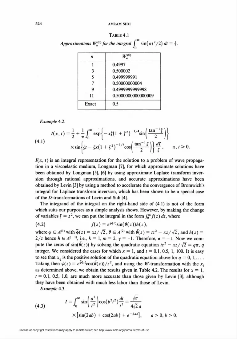
Example 4.1. /0°° sin(-¡rt2/2)/dt = 1/2. For this case u(t) = sin t, 9(x) =9(x) = (tt/2)x2, <b(x) = constant, and y = 0. Hence x¡, I = 0,1,..., are roots ofthe equation (tr/2)x2 = (I + l)v, 1 = 0,1,..., i.e., x, = ]¡2(l + 1), / = 0,1,....Since m = 2 and k = 0, we have a = -1. Therefore, xp(x) = cos(7rx2/2)/x andxp(xi) = (—l)'+x/x¡, 1—0,1,.... Table 4.1 contains some of the results of thecomputations for this integral.
License or copyright restrictions may apply to redistribution; see http://www.ams.org/journal-terms-of-use
524 AVRAM SIDI
Table 4.1f 00
Approximations Wf® for the integral I sin(wf 2/2) dt
/(x, í) is an integral representation for the solution to a problem of wave propaga-tion in a viscoelastic medium, Longman [7], for which approximate solutions havebeen obtained by Longman [5], [6] by using approximate Laplace transform inver-sion through rational approximations, and accurate approximations have beenobtained by Levin [3] by using a method to accelerate the convergence of Bromwich'sintegral for Laplace transform inversion, which has been shown to be a special caseof the /^-transformations of Levin and Sidi [4].
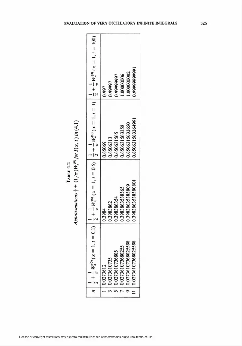
The integrand of the integral on the right-hand side of (4.1) is not of the formwhich suits our purposes as a simple analysis shows. However, by making the changeof variables f = z2, we can put the integral in the form /0°°/(z) dz, where
(4.2) f(z) = e^hin(9(z))h(z),where <b E Aw with 4>(z) = xz/ x/2,9 E A(2) with 8(z) = tz2 - xzf fl, and h(z) =2/z hence h E A{~X), i.e., k = 1, m = 2, y = -1. Therefore, o = -1. Now we com-pute the zeros of sin(0(z)) by solving the quadratic equation tz2 — xzf \/2 = q-n, qinteger. We considered the cases for which x = 1, and t = 0.1, 0.5, 1, 100. It is easyto see that xq is the positive solution of the quadratic equation above for q = 0,1,....Taking then xp(z) = e*(z)cos(0(z))/z2, and using the ^-transformation with the x,as determined above, we obtain the results given in Table 4.2. The results for x = 1,t = 0.1, 0.5, 1.0, are much more accurate than those given by Levin [3], althoughthey have been obtained with much less labor than those of Levin.
Example 4.3.
(4.3)= f°sinK" )cos(b2t2)-{ =
Jo \ t2 I t2 4{2a
x[sin(2a¿>) + cos(2ab) + e~2ab], a>0,b>0.
License or copyright restrictions may apply to redistribution; see http://www.ams.org/journal-terms-of-use
EVALUATION OF VERY OSCILLATORY INFINITE INTEGRALS 525
IIX
o
-I fe+
-les
IIH
SIt
-I fe+
-1rs
Ooo mONOn
m NO NOrS <S CS
>/"i ci ci o*o no ^O no
m ^i in iri »i^ tri m n n mno no no no no noo o o o o om >o in >i-> in u-ino no no no no NOo o o o o o
«i m mm N N INO O O Ooo oo oo ooNO NO NO NOci ci ci cir~ r-o o o
NO NOCl Clr- r-O oö ö
NO NO NO NOCl Cl Cl Clr^ r^ r^ r~M M n NO Od ö
o oO Ö
ci w*i t^ on —
License or copyright restrictions may apply to redistribution; see http://www.ams.org/journal-terms-of-use
526 AVRAM SIDI
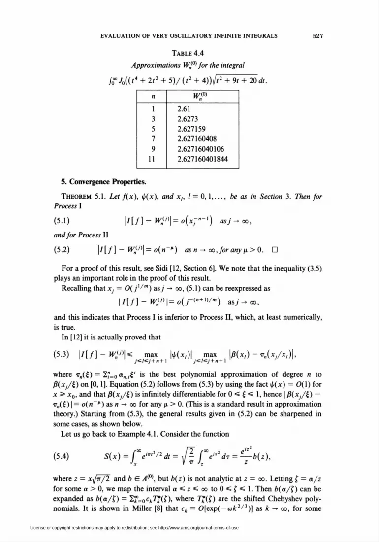
The integrand in this example has an infinite number of oscillations both as t -» ooand as t -» 0. Therefore we divide the range of integration into two: (0, T) and(T, oo). We then map the interval (0, T) to (1, oo) by the change of variable t = T/t,hence obtaining two infinite integrals whose integrands oscillate at infinity aninfinite number of times. For this example we take a = fW, b = fm ¡2 and T—l.With this choice of a, b, and T we have
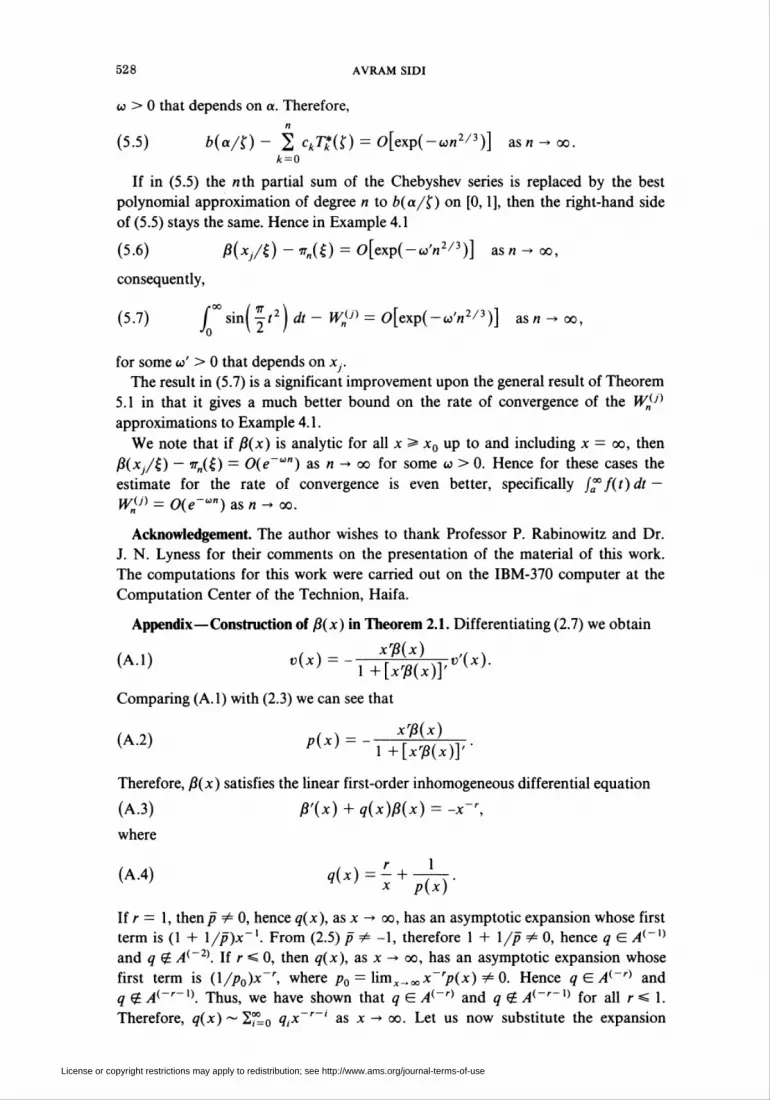
The exact value of this integral is not known to the author. This integral can be dealtwith by making use of the remarks at the end of Section 2.
First of all we have
9(x) = (x4 + 2x2 + 5)/ (x2 + 4),
<p(x) constant, and h(x) = /x2 + 9x + 20 in (2.20). Therefore, 8(x) = x2, i.e.,m = 2, k = 0, and y = 1. Consequently, the integrand is of the form
(4.6) f(x) = cos(x2)hx(x) + sin(x2)h2(x),
where A„ h2 E Am. Letting x, = \J(l + l)w, / = 0, 1,..., we have \p(x) =cos(x2)/x, hence ^(x,) = (—1)/+ '/x,, / = 0,1,_In Table 4.4 we give some of theresults obtained by applying the W-algorithm to the integral /.
License or copyright restrictions may apply to redistribution; see http://www.ams.org/journal-terms-of-use
evaluation of very oscillatory infinite integrals 527
Table 4.4Approximations Wj¡0) for the integral
/o°%(('4 + 2'2 + 5)/ (*2 + 4))]/t2+ 9t +20 dt.
n | WP1 2.613 2.62735 2.6271597 2.6271604089 2.62716040106
11 2.627160401844
5. Convergence Properties.
Theorem 5.1. Let fix), xp(x), and x,, I = 0,1,..., be as in Section 3. Then forProcess I
For a proof of this result, see Sidi [12, Section 6]. We note that the inequality (3.5)plays an important role in the proof of this result.
Recalling that x)■ = 0(jx/m) as j -> oo, (5.1) can be reexpressed as
|/[/l-^0)l=0(r("+1)/m,) as/ -oo,
and this indicates that Process I is inferior to Process II, which, at least numerically,is true.
In [12] it is actually proved that
(5.3) \l[f]-W<»\< max \xp(x,)\ max \ß(x,) - irH(xj/x,)\,j<Kj+n+\ y«/«/+n+l
where it„(£) = S"=0a„ ,£' is the best polynomial approximation of degree n toß(Xj/£,) on [0,1]. Equation (5.2) follows from (5.3) by using the fact xp(x) = 0(1) forx 3= x0, and that ß(xj/£) is infinitely differentiable for 0 < £ < 1, hence | ß(xj/£) —TTn(i) | = o(/i ,1) as n -> oo for any u > 0. (This is a standard result in approximationtheory.) Starting from (5.3), the general results given in (5.2) can be sharpened insome cases, as shown below.
Let us go back to Example 4.1. Consider the function
(5.4) S(x)=rei^/2dt=J- fV2dr = —b(z),Jx V 77 Jz Z
where z = xJm/2 and b E A(0\ but b(z) is not analytic at z = oo. Letting f = ot/zfor some a > 0, we map the interval a<z<ooto0<f<l. Then ¿>(a/f ) can beexpanded as b(a/$) = ~Zf=0ck7£(f), where r£(f) are the shifted Chebyshev poly-nomials. It is shown in Miller [8] that ck = 0[exp( — uk2/3)] as k -» oo, for some
License or copyright restrictions may apply to redistribution; see http://www.ams.org/journal-terms-of-use
If in (5.5) the nth partial sum of the Chebyshev series is replaced by the bestpolynomial approximation of degree n to b(a/$) on [0, 1], then the right-hand sideof (5.5) stays the same. Hence in Example 4.1
for some <o' > 0 that depends on Xj.The result in (5.7) is a significant improvement upon the general result of Theorem
5.1 in that it gives a much better bound on the rate of convergence of the W(J)approximations to Example 4.1.
We note that if ß(x) is analytic for all x > x0 up to and including x = oo, thenß(Xj/i) — tt„(Í) = 0(e"an) as n -* oo for some w > 0. Hence for these cases theestimate for the rate of convergence is even better, specifically f™f(t)dt —W¡¡j) = 0(e~un) as it -» oo.
Acknowledgement. The author wishes to thank Professor P. Rabinowitz and Dr.J. N. Lyness for their comments on the presentation of the material of this work.The computations for this work were carried out on the IBM-370 computer at theComputation Center of the Technion, Haifa.
Appendix—Construction of ß(x) in Theorem 2.1. Differentiating (2.7) we obtain
(A-l) v(x) = - ^ v'(x).i +[xrß(x)y
Comparing (A. 1) with (2.3) we can see that
xrß(x)(A.2) p(x) =
l+[xrß(x)y
Therefore, ß(x) satisfies the linear first-order inhomogeneous differential equation(A.3) ß'(x) + q(x)ß(x) = -x~r,
where
(A.4) q(x) = z +x p(x)'
If r = 1, then/j ¥= 0, hence ^(x), as x -» oo, has an asymptotic expansion whose firstterm is (1 + l/^)x_1. From (2.5) p ¥= -I, therefore I + l/p¥= 0, hence q £ A(~X)and q E A(~2\ If r < 0, then ¿¡r(x), as x -» oo, has an asymptotic expansion whosefirst term is (l/p0)x~r, where p0 = limx^ocx~rp(x) =£ 0. Hence qEA(~r) andq £ A(~r~X). Thus, we have shown that q £ A(~r) and q £ A{~r~X) for all r =s 1.Therefore, q(x) ~ 2°L0 ^r,x~r~' as x — oo. Let us now substitute the expansion
License or copyright restrictions may apply to redistribution; see http://www.ams.org/journal-terms-of-use
EVALUATION OF VERY OSCILLATORY INFINITE INTEGRALS 529
ß(x) ~ 2°L0 ßj/x' in (A.3). We can easily see that ß0 = -l/q0. The coefficientsßx, ß2,..., can now be determined by solving the recursion relation obtained from(A.3).Computer Science DepartmentTechnion—Israel Institute of TechnologyHaifa, Israel
1. F. B. Hildebrand, Introduction to Numerical Analysis, McGraw-Hill, New York, 1956.2. D. Levin, "Development of non-linear transformations for improving convergence of sequences,"
Internat. J. Comput. Math., v. B3, 1973, pp. 371-388.3. D. Levin, "Numerical inversion of the Laplace transform by accelerating the convergence of
Bromwich's integral," J. Comput. Appl. Math., v. 1, 1975, pp. 247-250.4. D. Levin & A. Sidi, "Two new classes of non-linear transformations for accelerating the
convergence of infinite integrals and series," Appl. Math. Comput. (In press.)5. I. M. Longman, "Numerical Laplace transform inversion of a function arising in viscoelasticity," J.
Comput. Phys., v. 10, 1972, pp. 224-231.6. I. M. Longman, "On the generation of rational approximations for Laplace transform inversion
with an application to viscoelasticity," SIAMJ. Appl. Math., v. 24, 1973, pp. 429-440.7.1. M. Longman, private communication, 1979.8. G. F. Miller, "On the convergence of the Chebyshev series for functions possessing a singularity in
the range of representation," SIAMJ. Numer. Anal., v. 3, 1966, pp. 390-409.9. A. Sidi, "Convergence properties of some nonlinear sequence transformations," Math. Comp., v. 33,
1979, pp. 315-326.10. A. Sidi, "Some properties of a generalization of the Richardson extrapolation process," J. Inst.
Math. Appl., v. 24, 1979, pp. 327-346.H.A. Sidi, "Analysis of convergence of the ^-transformation for power series," Math. Comp., v. 35,
1980, pp. 833-850.12. A. Sidi, "Extrapolation methods for oscillatory infinite integrals," /. Inst. Math. Appl., v. 26, 1980,
pp. 1-20.13. A. Sidi, "An algorithm for a special case of a generalization of the Richardson extrapolation
process," Numer. Math. (In press.)
License or copyright restrictions may apply to redistribution; see http://www.ams.org/journal-terms-of-use