the transmission of superheated steam over long distances

THE TRANSMISSION OF SUPERHEATED STEAM OVER LONG DISTANCES

By Professor L. F. C. A. Genkve, BSc., M.1.Mech.E."

The aim of the paper is to obtain as accurate a solution as possible to problems arising in the transmission of superheated steam over long distances for (a) industrial heating and (b ) power generation. After a general survey, with a description of two typical installations, the problem is discussed under headings (a) and (b), and the usual practice in fixing steam velocities is given. The present state of knowledge of radiation losses is reviewed; first, the standard English practice of using a coefficient based on the pipe surface and varying with the thickness of the insulating material; and second, the method, used mainly in America, which involves conductivity coefficients. The effect of air currents on heat loss is investigated and a new equation is deduced for the equivalent velocity past the pipe, due to natural convection.

Standard formulz for the coefficient of friction and the viscosity of steam are discussed; for the former a new formula of the rectangular hyperbola type is derived from Carnegie's results and corrected for roughness. Steam viscosity is considered in the light of Speyerer's and Sigwart's investigations ; curves of Sigwart's results are plotted on a convenient base of logarithms of pressures.

Conditions during flow in a horizontal straight pipe with perfect insulation are considered and new equations, simplifying the problem, are derived from the fundamental equations.

The author treats from a new viewpoint the problem of puwer transmission by steam over long distances, based on the loss of available Rankine heat drop. Numerical examples are worked out, as also is the effect of air currents on the coefficient of heat loss. Finally the limiting factors, including the effect of radiation losses, in the long-distance transmission of steam are analysed and their practical importance is discussed.

INTRODUCTION The use of steam as a medium for supplying heat to buildings and

to industrial appliances has now been established for many years. Originally, the main reasons for using steam heating in preference to direct heating by the combustion of fuels were convenience, safety, ease of regulation, cleanliness, and especially the possibility of supplying the heat at constant temperature by condensation of the steam ; but, owing to the inefficient design of the low-pressure boilers then used, and the poor insulation of the transmission piping, the cost of heating by steam was comparatively high.

I t was not long, however, before engineers realized the possibilities -~

* Faculty of Engineering, Egyptian University, Giza, Egypt. CI.Mech.E.1

at PENNSYLVANIA STATE UNIV on February 20, 2016pme.sagepub.comDownloaded from

http://pme.sagepub.com/

356 TRANSMISSION OF STEAM OVER LONG DISTANCES

of utilizing the exhaust from steam engines for heating purposes ; the steam, generated in better-designed boilers at a higher pressure than required for heating only, was used to drive reciprocating engines, converting in this way a small fraction of its total heat into work. After being thoroughly cleansed of any oil in special oil-separating apparatus, it was passed through the various heating appliances, where it gave up the greater part of its remaining total heat, mainly as latent heat of condensation. Finally, as much of it as could be recovered was pumped back to the boilers as feed water. With the advent of steam turbines, the problem of removing the oil disappeared ; and correct and thorough insulation of the transmission piping helped to increase the economy of the process.

The problem of supplying steam for variable power and variable heating demands was met by the use of back-pressure and steam- extraction turbines and steam accumulators ; and there are nowadays many plants operating under these conditions with a very high proportional utilization of the heat generated in the boilers by the fuel. The development of the modern high-output central steam station has led to the construction of steam generating plant of very high efficiency operating with pressures varying from 450 lb. per sq. in. to 1,900 Ib. per sq. in. ; and engineers have in the last ten years given serious consideration to the problem of tapping these very efficient installations for their supplies of steam for heating and for industrial processes.

Several practical solutions of the problem have been embodied in modern industrial plants, depending on the nature and size of the plants and on their location with regard to existing power stations. Thus, in industrial works of very large size, the tendency is towards the installation of independent plant, comprising high-pressure boilers and “back-pressure” turbines-or, alternatively, extraction (“bleeder”) turbines-which generate the main power with the high-pressure steam, and supply steam at lower pressures for operating the special process machinery, and for heating purposes.

On the other hand, plants of small or medium size which are established in the neighbourhood of large steam stations may receive their electrical power by transmission lines and their steam supply by long pipe lines from back-pressure or extraction turbines in the station; or again, they may receive a supply of steam directly from the high- pressure boilers of the central station and generate their own power in such turbines, using the exhaust or extraction steam for the process work. In most cases, such installations necessitate the transmission of steam over quite long distances, ranging from a few hundred feet to over 5,000 feet ; and it is the purpose of the present paper to examine some of the problems of such transmission.



TRANSMISSION OF STEAM OVER LONG DISTANCES 357

An outstanding example of a very large industrial plant is that installed at the Billingham synthetic ammonia and nitrates works of Imperial Chemical Industries (Humphrey, Buist, and Bansall 1930).* Briefly, this plant consists of eight three-drum pulverized-fuel boilers, each designed to operate normally at an output of 215,000 Ib. of steam per hour. The normal saturated steam pressure is 715 lb. per sq. in. abs., but the supply pressure to the high-pressure distributing receiver is 675 lb. per sq. in. abs., the maximum steam temperature being 458 deg. C. ; and the steam is supplied to three 12,500 kW. back-pressure turbines exhausting at 290 lb. per sq. in. abs. and 345 deg. C. into a low-pressure receiver from which it is passed to (a) process plant steam mains and (h) two 12,500 kW. condensing turbo-alternator sets. From the latter the steam is wholly extracted and is used in four feed- water heaters and in an unusually large quadruple-effect distillation plant which supplies make-up feed water to the boilers. The low- pressure receiver is equipped to act as a desuperheater for any steam passed directly to it through a reducing valve from the high-pressure line. There are altogether seven feed heaters, and the feed temperature at inlet to the Foster steaming economizers is 205 deg. C.

The total steam output of the boilers is 11,900,000 kg. per day, of which 6,930,000 kg., or about 57 per cent, is used for the process plants. About 42 per cent of this amount-i.e. about 24 per cent of the total output-cannot be recovered, hence the large capacity of the distillation plant installed. The maximum distance of transmission of steam in this plant is stated to be 1 mile, both for the high-pressure (290 lb. per sq. in.) steam and for a 30 lb. per sq. in. low-pressure supply. The 290 Ib. per sq. in. process plant steam is utilized in driving non-condensing reciprocating engines and turbines, the exhaust from which is used for heating purposes in evaporation vats. A number of mixed-pressure turbines serve to maintain a balance between power and heating steam requirements. The sizes of the steam mains are 7,9, and 10 inches internal diameter for the 715 lb. per sq. in. lines, and 12t inches internal diameter for the 290 lb. per sq. in. lines; the insulation consists of 1 inch of asbestos, 24 inches of magnesia composition, and a covering off inch of hard-setting cement-a total thickness of 4 inches.

An American plant of considerable interest from the point of view of process steam supply is the Deepwater steam station erected on the east bank of the Delaware river in New Jersey (Power Plant Engineer- ing 1929). This station is run in the joint interests of three large companies, each of which has its own plant in the central building.

* An alphabetical list of references is given in the Appendix, p. 400.




The first two-which are power supply companies-have cross- compound turbo-alternator condensing units, each of 53,600 kW. capacity, supplied from a pair of Babcock and Wilcox boilers (one standard and one reheat) with steam at 1,215 Ib. per sq. in. abs. and a temperature of 385 deg. C.

The third company-the Du Pont de Nemours Company-has a high-pressure turbine of 12,500 kW. capacity, identical in size and construction with the high-pressure turbines of the two larger sets. It is also supplied with steam at 1,215 lb. per sq. in. abs. and 385 deg. C. from two standard Babcock and Wilcox boilers and the whole of the power generated is delivered to the Du Pont Company. At normal load, this turbine exhausts 530,000 Ib. of steam per hour at 400 lb. per sq. in. abs. into seven single-effect high-pressure evaporators, which in turn provide hourly 400,000 lb. of steam at 180 Ib. per sq. in. abs. from raw water. This medium-pressure steam is superheated to 227 deg. C . by live-steam reheaters and delivered by two 16-inch mains, 1,500 feet long, to the works of the Du Pont Company. The exhaust steam from the turbine is completely condensed in the evaporators, and returned directly by centrifugal pumps to the suction of the boiler feed pumps.

The object of this rather unusual arrangement is to avoid the necessity of pumping back from the Du Pont works any condensate that might be available from the process plants. This has the disadvantage of requiring the use of evaporator plant of large capacity, and of reducing considerably the available Rankine heat drop of the steam through the reduction of pressure. The latter point is not, however, of great importance if the steam is used wholly for heating purposes. The Du Pont plant is interconnected with the systems of the two other companies. Should the process steam requirements necessitate the turbine working at full load, the excess power generated is supplied to the other electrical systems ; on the other hand, if the steam requirements are low and the electrical power developed in the turbine in consequence insufficient, the deficiency can be made up from the other power systems.

Layout of New Plant. Where a new industrial centre is being developed, there is no doubt that the ideal layout would comprise a centrally placed steam generating station supplying both electrical power and steam to the surrounding factories and works, which should be erected within a radius of about 1 mile from the station. Possible schemes of operation would be as follows.

(a) The surrounding factories can be considered as forming one group, and special back-pressure turbines can be installed in the station working with high-pressure steam and supplying steam at




medium pressure-but considerably higher than the steam pressures required in the process work-to the factories. These turbines would take care of the electrical base load for the group, the local electrical peak loads being dealt with in the factories themselves by small back- pressure or extraction units operated from the medium-pressure steam transmission line, and exhausting into lower-pressure process steam lines or into a low-pressure steam accumulator. The larger units of the process machinery should in this case be directly driven by back- pressure turbines.

( b ) With all-electric drives in the factories, the whole of the power units can be erected in the main station, and the heating steam transmitted through pipe lines at pressures slightly higher than those required for the process work. The power units would then be extraction condensing or mixed-pressure turbines with automatic regulation for dealing with fluctuating steam and power demands, High-pressure accumulator plant might also be embodied in this scheme.

(c ) A third scheme might provide only the high-pressure boiler plant in the central station, designed for maximum efficiency, and transmitting high-pressure steam direct to the various factories. Each factory would then have its own equipment of back-pressure and extraction turbines, combined with suitable accumulators in such a way as to meet the heating steam and power requirements in the best possible way. By a judicious combination of the load curves of the various factories, the central boiler plant could be operated continuously day and night at nearly constant load.

In all the above schemes and others of a similar nature, it is of course necessary to pump back to the main boiler plant as much condensate as possible from the various factories, in order to reduce the capacity of the evaporators required for the boiler feed make-up. In order not to forgo the advantages of heating the boiler feed by extracted steam, special feed-heating turbines of the extraction or back-pressure type can be installed in the power station. In scheme (c), these could deal with, say, the lighting load only of the group of factories.

It is impossible to state definitely which of the three schemes suggested is the best; only by a very careful comparison of capital and working costs can a correct decision be arrived at. Broadly speaking, scheme (a) involves the use of both electrical transmission and long steam piping, both, however, of medium capacity, as only the electrical base load is carried and the steam pressure is fairly high. It has been adopted, with various modifications, in a number of modern installations mainly because of the moderate pressures in the transmission pipe lines, and because of the advantage of dealing with the base load for the



3 60 TRANSMISSION OF STEAM OVER LONG DISTANCES

group by means of a single large machine in the main station. I t is not, however, very flexible from the point of view of an extension of the system, say, by the inclusion of other factories in the group.

Scheme ( b ) is by far the simplest, and probably the cheapest in capital cost, as it requires only a few large turbo-generators in the main station, and the cost of extra buildings for housing power plant in the factories is eliminated. Supervision and maintenance costs will be a minimum. The cost of the electrical transmission lines and also of the low-pressure steam mains will, however, be much higher, and the efficiency of the system will be lower, chiefly owing to the reduced efficiency of the steam transmission at low pressures, and to the electrical transmission losses which affect the whole of the power supply. This scheme is also very inelastic with regard to moderate extensions ; thus, if one more factory is to be included in the group, a new unit of small capacity has to be introduced in the station, and this is, of course, against the fundamental principle of the scheme.

Scheme (c) is probably the most efficient in operation, as it eliminates all electrical transmission losses, and supplies steam for power and process work with the minimum amount of loss in the high-pressure pipe line. I t has not been adopted to any extent, however, mainly owing to the objection of industrial engineers to high-pressure steam. Further, in a group scheme, it means that each factory must have its own power building and units ; in consequence a number of smaller machines, of somewhat lower efficiency than one or two large machines, will have to be installed, and the aggregate cost will be higher. Main- tenance and supervision costs will also be higher. The cost of the electrical transmission lines is, however, eliminated, and that of the steam lines much reduced. Also, since each factory contains its own power units, the addition of any single factory to the group entails only a fresh steam line from the main station, and increased boiler capacity ; in many cases the latter can be obtained merely by a small increase in the rate of steaming of each boiler, a contingency which is usually provided for in modern boiler plant which has a high overload capacity.

The quality or condition of the steam supplied to the steam transmission lines depends on the way in which it is to be utilized at the factory end. For heating appliances, the maintenance of a supply of heat at constant temperature is essential ; hence the steam is almost invariably supplied in approximately the dry saturated state, and drained from the heaters as soon as it is condensed. The pressure of the supply is usually low, depending on the temperature that it is desired to maintain in the heaters, generally between about 200 lb. per sq. in. and a few pounds per square inch above

Quality of Steam Supply.




atmospheric. For long-distance transmission, the steam is supplied to the mains with just enough superheat to enable it to reach the other end in a slightly superheated condition ; and its pressure at inlet is just high enough to allow for the pressure drop in the pipe line due to friction.

It must be stated here that the losses in the case of a saturated steam supply are very high, owing, first, to condensation, since the reheating effect of friction is insufficient to balance the usual radiation loss ; and second, to the increased friction due to the high viscosity of the water film deposited on the walls of the pipe. For power purposes, on the other hand, the steam must be supplied at high pressures ; and the amount of superheat imparted to it must be such that either its wetness at the low-pressure stages, when it is used in condensing turbines, is not excessive ; or it is exhausted into the low-pressure process mains approximately dry saturated, when used in extraction or back-pressure turbines.

It is a well-known fact that, for a given total steam temperature, the higher the initial pressure, the greater will be the wetness of the steam when expanded adiabatically to a given pressure ; hence when steam at very high pressures-over 800 lb. per sq. in.-is used in condensing turbines, it is the standard practice (mainly in America, where such high pressures are now quite common) to resuperheat the steam at an intermediate stage in live-steam or flue gas reheaters. All these factors have to be borne in mind when deciding on the initial pressure and temperature of the steam supply ; but one essential condition for efficient transmission over long distances is that the steam must not become wet at any point, and must therefore be suitably superheated at the start.

Losses in Long Steam P;Pes. The losses in long steam pipes can be considered from two distinct points of view: (1) the loss in total energy; (2) the loss in Rankine, or adiabatic, heat drop.

Assuming a straight horizontal pipe, this loss is measured solely by the amount of heat lost by radiation and convection from the surface of the pipe or its lagging. The work done against the frictional resistances internally is returned to the steam, and hence, were it not for the radiation loss, the total energy would remain the same. But, owing to the pressure drop (due to the work done against friction), and the consequent increase in specific volume, the velocity of flow increases, so that the heat energy actually decreases, whilst the kinetic energy increases. Usually this kinetic energy is reconverted into heat when the steam enters the receiver or steam distributor at the outlet end of the pipe.

It is to be noted here that, in the case of steam transmitted entirely

(1) The Loss in Total Energy.




for use in heaters, it is the total energy that finally counts, and hence the pipe line can be designed for a high-pressure drop and a high velocity of flow, since the friction work will be reconverted into heat. By so doing, the cost of the piping and lagging will be reduced, and also the total radiation loss. With the very efficient forms of modern pipe lagging now in use, this radiation loss can be kept very low indeed, and the efficiency of total energy transmission for a distance of over 1 mile may be as high as 98 to 99 per cent.

This represents the heat available for conversion into work in an engine or turbine, and is very important in the case of long-distance transmission to power generating units. The calculation of this loss is a simple one if the initial and final conditions of the steam are known, and if a lower temperature or pressure limit is fixed as a basis. In such a case, the pressure drop should be kept as low as possible ; this means allowing lower velocities of flow in order to reduce the friction loss. In practice, a loss of about 4-10 per cent of the available Rankine heat drop may be expected in distances from 2,000 to 5,000 feet.

Steam flow velocities are usually fixed in a very arbitrary fashion ; various authorities merely state certain approximate values, generally related to the size of the steam pipe to be used. Probably as good an empirical rule as any for the comparatively short runs of piping between boiler and turbine in power stations is the one given by Gebhardt (1925) ; it is as follows : 1,000-1,250 ft. per min. per inch of internal diameter of the pipe, the higher figure being used for pipes of 12 inches diameter and over. These figures are for fairly straight runs of piping with few bends and valves ; where many bends and valves occur, 80 per cent of the above values should be taken.

In the discussion on a paper by Carnegie (1930), several interesting statements were made concerning the best steam velocities. Mr. W. F. Carey stated that for the 123-inch mains at Billingham, carrying steam at 290 lb. per sq. in. abs. and 320 deg. C . , the “economic speed” was found to be 100 ft. per sec., and that this speed was, in general, independent of the pipe diameter ; whilst for 16-inch mains with saturated steam at 30 lb. per sq. in. abs., it was 60 ft. per sec. Mr. Carnegie, in his reply, pointed out that at Billingham the steam was used for power production, and that low velocities were thus required ; but that for steam to be consumed only in heaters he would have no hesitation in using velocities of over 300 ft. per sec. These values are, of course, initial values.

Roughly speaking, therefore, it appears that, for power purposes initial velocities of superheated steam for long-distance transmission should not greatly exceed 100 ft. per sec., whatever the diameter of the

(2) The Loss in Rankine, or Adiabatic, Heat Drop.




pipe ; and that for heating purposes much higher velocities are preferable. Also that very much lower velocities should be used for saturated steam mains.

The figures given above are convenient as a rough guide, and should not be assumed for calculations of long-distance transmissions. In any particular case, in fact, the velocity of flow should be arrived at from a consideration of other more important factors, such as the allowable total pressure drop, or the allowable loss of available heat drop. A method of solving piping problems from these aspects will be worked out later in the paper.

The investigations that follow cover only the Aow of superheated steam in straight pipes ; the effect of bends, valves, etc., can be allowed for in the usual manner by adding “equivalent lengths of straight piping”-calculated from various empirical formulae-to the actual length of straight piping.

GENERAL CONSIDERATIONS

The units used throughout the following investigation will be the standard English units of mass and length, namely, the pound and the foot, and the Centigrade scale of temperature. The unit of heat will therefore be the Centigrade Heat Unit (C.H.U.).

Symbolic Notation :- J Joule’s equivalent, 1,400 ft.-lb. per C.H.U. P Pressure, pounds per square foot. V Specific volume, cubic feet per pound. T Absolute temperature, degrees Centigrade. t Temperature, degrees Centigrade. L Latent heat, C.H.U. per pound. E Internal energy, C.H.U. per pound. I Total heat, C.H.U. per pound=E+PV/J. 4 Entropy, per pound. Q Quantity of heat, C.H.U. per pound. M Mass flow, pounds per second. D Internal diameter of pipe, feet. A Cross-sectional area of pipe, square feet. A Length of pipe, feet. U Mean velocity of flow, feet per second. p Specific density, pounds per cubic foot=l/V. p Absolute viscosity, poundal-seconds per square foot. R Reynolds’s Number. f Coefficient of friction.




K

/3

C1, C,, etc. Constants.

Thermal conductivity, C.H.U. per hour per square foot per inch thickness per degree Centigrade temperature difference. Heat loss coefficient, C.H.U. per hour per square foot per degree Centigrade temperature difference.

When a homogeneous fluid flows in a straight pipe of uniform cross- section, the effect of a transfer of heat between the fluid and external bodies is to cause an alteration in the pressure, specific volume, temperature, total heat, and velocity of flow in the pipe. The changes produced can easily be calculated, provided the rate of heat transmission to or from the fluid is known, and provided also that no other factor affects the flow.

In all actual cases of flow, however, there are a number of such factors, the most important being the effect of gravity when the axis of the pipe is inclined to the horizontal, and the sum of the internal resistances to flow referred to under the general term “friction”. The effect of gravity is completely defined when the inclination of the pipe is known, and can be dealt with exactly in the flow equations. The frictional resistances comprise “internal” or molecular friction of the fluid, and boundary friction at the internal surface of the pipe.

According to Osborne Reynolds, the total internal friction is depen- dent on two distinct viscosities. One is “a physical property of the fluid and is a measure of the instantaneous resistance to distortion at a point moving with the fluid” (Stanton 1923). Newton defined this viscosity pl by considering the fluid to be moving in parallel layers with velocities u at distances y , measured at right-angles to the direction of flow, from the enclosing surface. Under these conditions, at any point, Fl , the internal frictional force per unit area is equal to the shearing stress ; also

Shearing stress=pldu/dy.

The other viscosity is a “mechanical” viscosity pz arising from the “molar motion of the fluid and given by the relation F2=p2dzi/dy, where zi is the mean motion at a point, taken over a sufficient time, and p2 is a function of ti and probably also of the solid boundaries of the fluid” (Stanton 1923). This mechanical viscosity can only be present in what is known as “turbulent” flow, of which Stanton remarks that “although the mean motion at any point taken over a sufficient time is parallel to the sides of the channel, it is made up of a succession of motions crossing the channel in different directions”.

Experimental determinations of absolute viscosity are generally carried out with low velocities and smooth boundary surfaces, i.e. under conditions of sinuous flow, so that the coefficients of absolute viscosity




given in textbooks for various fluids are really values of the “physical” viscosity of Osborne Reynolds and Newton.

The frictional resistance to flow at the boundary surface of a pipe depends upon a very indefinite factor known as the roughness of the pipe. Not very successful attempts have been made to establish scales of surface roughness by experiments on pipes roughened internally by tool marks of varying coarseness ; and the problem is further complicated by the fact that, for a given surface roughness, the actual factor or coefficient of roughness-as affecting the resistance to flow-is a function of the reciprocal of the pipe diameter. Broadly speaking, solid- drawn steel, brass, copper, and lead pipes of small diameters in unbroken lengths, and glass tubing, are considered “smooth”. Commercial wrought iron, steel, and cast iron piping, and any pipe made up of short lengths with flanged joints, must be taken as being “rough”.

In practice, the total frictional resistance in flow problems is dealt with by introducing in the formulae for pressure drop a coefficient of friction chosen in each particular case from the results of experiments on pipes or channels as nearly as possible similar to the one considered. This coefficient of friction (denoted by f ) is a dimensionless number, but its value depends on the form of the pressure drop formula adopted. For the purposes of this investigation, the pressure drop formula will be used in the form

m being the hvdraulic mean diameter D, tde formula becomes

depth. So for a circular pipe of internal

SP - 2juz,, --- P gD

For smooth pipes, or pipes of the same roughness factor, the value off depends on the velocity, density, and viscosity of the fluid, and on the internal diameter of the pipe. It has been shown by Osborne Reynolds that, for given conditions, f can be expressed as a function of pUD/p, a quantity which has no dimensions, and is therefore the same in any consistent system of units. This quantity is generally called the Reynolds Number, and will be denoted by R.

It can readily be seen, from the above considerations, that the pre- dikion of the coefficient of friction for any particular case can never be an exact process ; a reasonable estimate of its value can, however, be made from an examination of the numerous experiments which have been carried out on pipe friction. A very useful study of most of this experimental work will be found in Schule’s “Technical Thermo-




dynamics” (1933), the main results being embodied in a series of curves off plotted against R. From these curves, various formulae have been established connecting f and R, some of which are considered later. Such formulae have the great advantage that they are applicable to any fluid, flowing, however, in pipes which have the same smoothness or roughness factors as those from which the formulz are derived.

The value of the absolute viscosity p to’be used in the expression for R can be found for moderate temperatures and low pressures from the various established formulae for water, oils, and many gases. Until recently, very little was known of the values of p for steam at high temperatures and pressures ; researches carried out on the Continent in the last few years have, however, done much to fill this gap in our

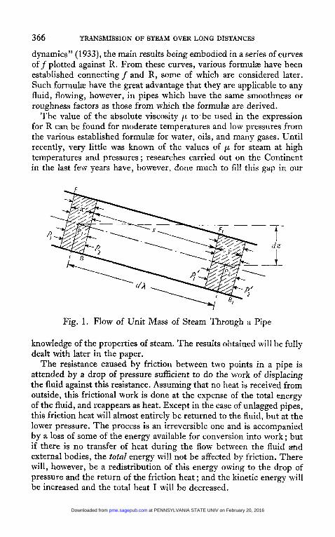
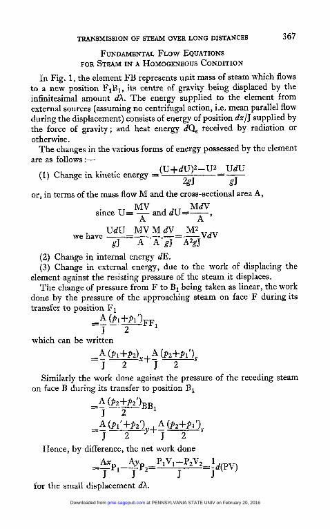
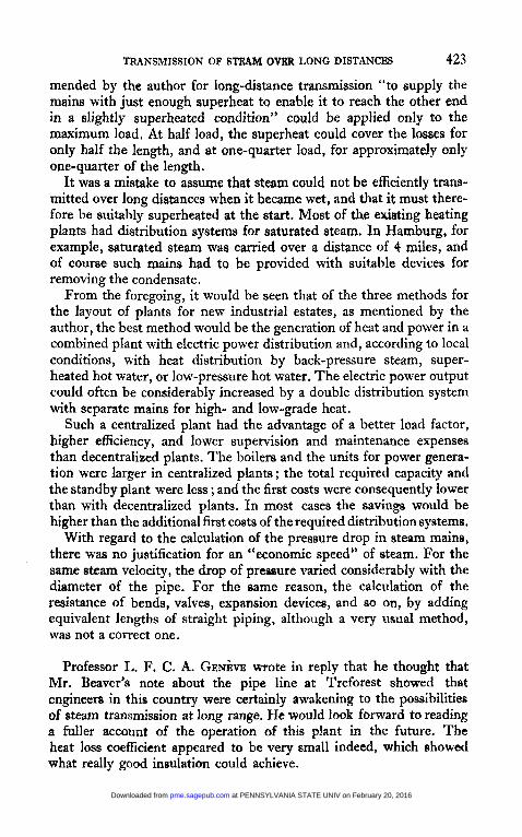
Fig. 1. Flow of Unit Mass of Steam Through a Pipe

knowledge of the properties of steam. The resuIts obtained will be fully dealt with later in the paper.

The resistance caused by friction between two points in a pipe is attended by a drop of pressure sufficient to do the work of displacing the fluid against this resistance. Assuming that no heat is received from outside, this frictional work is done at the expense of the total energy of the fluid, and reappears as heat. Except in the case of unlagged pipes, this friction heat will almost entirely be returned to the fluid, but at the lower pressure. The process is an irreversible one and is accompanied by a loss of some of the energy available for conversion into work ; but if there is no transfer of heat during the flow between the fluid and external bodies, the total energy will not be affected by friction. There will, however, be a redistribution of this energy owing to the drop of pressure and the return of the friction heat ; and the kinetic energy will be increased and the total heat I will be decreased.



TRANSMISSION OF STEAM OVER LONG DISTANCES

FUNDAMENTAL FLOW EQUATIONS FOR STEAM IN A HOMOGENEOUS CONDITION

In Fig. 1, the element FB represents unit mass of steam which flows to a new position FIBl, its centre of gravity being displaced by the infinitesimal amount dA. The energy supplied to the element from external sources (assuming no centrifugal action, i.e. mean parallel flow during the displacement) consists of energy of position dz/J supplied by the force of gravity; and heat energy dQ, received by radiation or otherwise.

The changes in the various forms of energy possessed by the element are as follows:-

367

(U+dU)2-U2_UdU (1) Change in kinetic energy = _- 2gJ gJ

or, in terms of the mass flow M and the cross-sectional area A, MV MdV

since U= - and dU=- A A ’

UdU M V M ~ M2 we have -=-.-.-==---VdV gJ A A gJ A2gJ

(2) Change in internal energy dE. (3) Change in external energy, due to the work of displacing the

element against the resisting pressure of the steam it displaces. The change of pressure from F to B, being taken as linear, the work

done by the pressure of the approaching steam on face F duringits transfer to position F1

which can be written

Similarly the work done against the pressure of the receding steam on face B during its transfer to position B1

Hence, by difference, the net work done

for the small displacement dx.




The energy required to overcome the frictional resistances =fUzdX/2gJrn. It is assumed that the whole of this energy has been returned to the element as heat by the time it has reached its new position FIB1.

The total energy of the element has now been increased by the amounts received from external sources only, and hence the following equation is obtained :-

. . . . +dQ, (1) d(PV) UdU dz dE+- +-=-

J gJ J and, since d I = d E + d o , we have finally

J UdU dz dI=-- +-+dQ, . . . . . . (2) gJ J

Furthermore, independently of the motion of the element as a whole, the change in the values of P, V, and E for the steam is due entirely to the heat added to it, both from external sources and from the conversion of the friction work into heat.

We have therefore, by the first law of thermodynamics,

(3) fU2dh PdV V6p dQ=dQe+-=dE+-=dI-- . . . . 2gJm J J

Equations (1)-(3) are applicable to any pipe or conduit of uniform or variable cross-section, provided centrifugal action on the steam is absent, i.e. that the axis of the pipe is straight.

A further relation, known as the equation of continuity, gives : M=mass flow per unit time=AU/V=AUp=constant at any section of the pipe, provided there is steady flow without longitudinal pressure

Considering now only pipes of uniform diameter, with the axis . . . . . . . . . . . . . . . . . . . waves (4)

horizontal, the following fundamental equations are obtained :- 7TD2 4

From the equation of continuity, since A= -=constant,

( 5 ) M 4M U

V A .rrD2 . . . . . -=up=-=-=c~.

From equations (2) and ( 5 ) , putting dz=O,

dI=-- C12VdV+dQ, (6) . . . . . . gJ

From equations (3) and (9, putting m=D/4,

(7) . . . . . VdP J

dh=dI-- 2fV2cp dQ,+ -

SDJ




and, combining equations ( 6 ) and (7),

C 2 2fv2c12dA= - -!-VdV-VdP . . . gD g

or, in another form,

(9) dP C,2- 2fC1* VdA -+---- - dV g g D ' V d . * . * *

Before applying these fundamental relations to the solution of problems of superheated steam flow, it is necessary to consider two factors in some detail, namely, the radiation loss and the coefficient of friction.

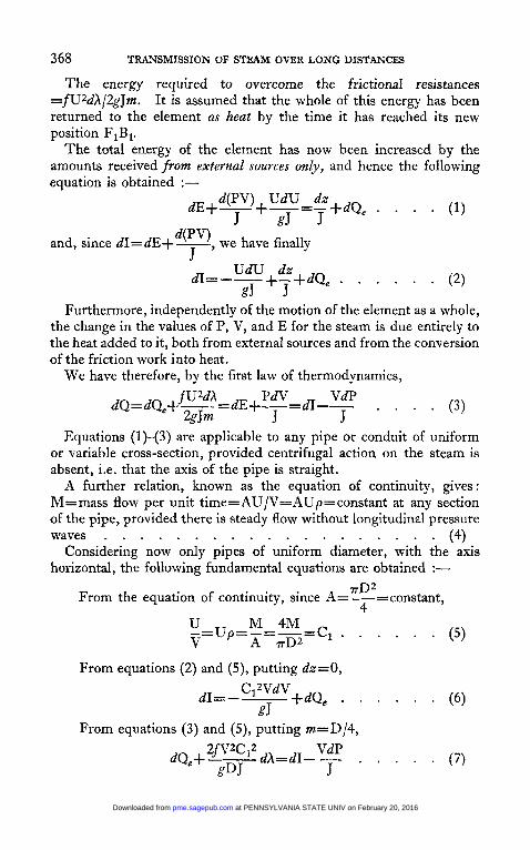
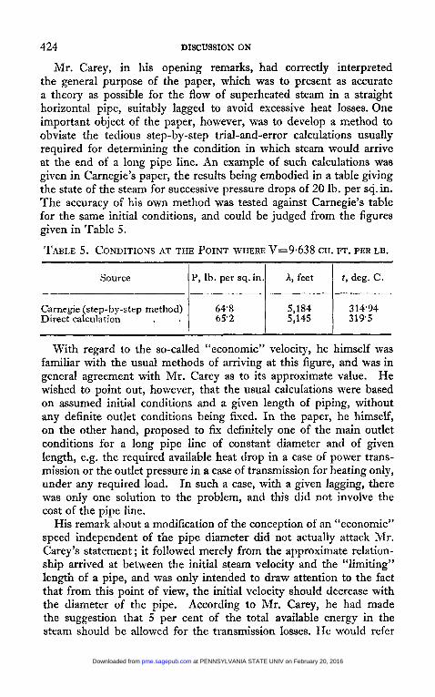
Fig. 2. Temperature Difference between Pipe Surface and Air 85 per cent magnesia composition; air temperature, 21 deg. C.

The Radiation Loss. The term covers the heat loss both by radiation and by convection from the surface of the pipes or of their lagging; allowance is made for this loss in the fundamental equations by the quantity dQ,, which is therefore invariably negative. Numerous experiments have been carried out to determine the radiation loss for varying thicknesses of the most usual insulating materials on the market. Makers of such materials provide tables and curves of the properties of their products, such as the conductivity at various mean temperatures, the loss of heat per hour per unit area of the pipe for a series of lagging thicknesses and temperature differences between

25 at PENNSYLVANIA STATE UNIV on February 20, 2016pme.sagepub.comDownloaded from



the pipe surface and the atmosphere, the efficiency or percentage saving of heat loss over bare piping with these thicknesses, and so on.

In England, the standard practice is to use coefficients which represent for various lagging thicknesses the heat loss per hour per square foot of the pipe surface per degree difference of temperature between the pipe and the atmosphere. For example, the curves in Fig. 2 (based on experiments carried out at the National Physical Laboratory, Eng- land, on ordinary 5-inch diameter wrought iron piping with oxidized surface, and reported in Carnegie’s paper (1930) previously referred to) show the values of these coefficients for the most generally used steam pipe lagging material, namely, the “85 per cent magnesia composition”,

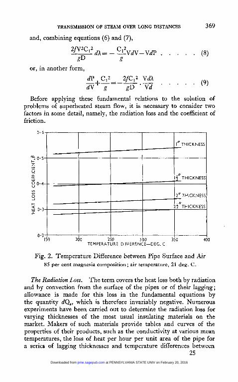
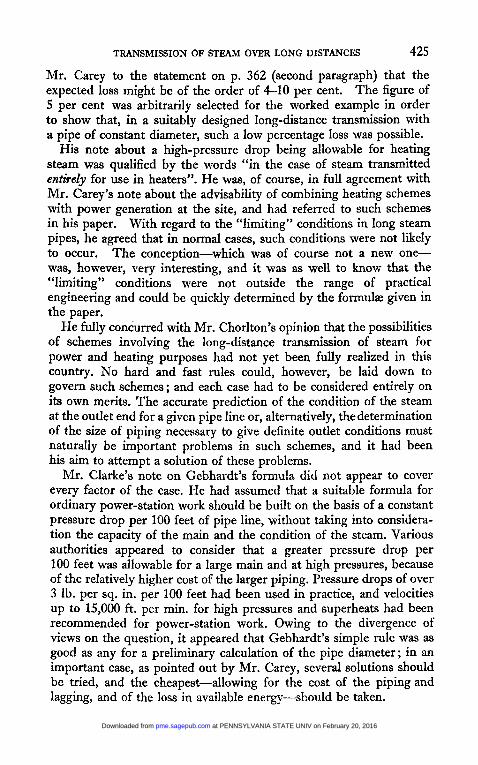
Fig. 3. Temperature Difference between Pipe Surface and Air Air temperature, 21 deg. C.

which consists of a mixture of 85 per cent hydrated carbonate of magnesia with 15 per cent asbestos fibre for bonding purposes. This material is used in paste form, or it may be obtained in moulded segmental lengths of about 3 feet for all standard pipe sizes. It can be applied directly to the piping for temperatures below 250 deg. C. Above this, a coating of special heat-resisting material should be first applied to the pipe to prevent deterioration of the outer layer of magnesia insulation.

The material mostly used for this heat-resisting layer is a mixture of the so-called diatomaceous earth, consisting mainly of silica in the form of remains of microscopic organisms, with asbestos as a bond. The natural earth is stratified, and must be crushed and calcined before being mixed with the bonding material and moulded. Fig. 3 shows the heat loss coefficients for two combinations of heat resisting “diatomite” and




85 per cent magnesia composition, with an outer weatherproof coating of hard-setting cement.

Steam pipe insulation of this kind is not mechanically strong, and so it is generally finished outside with a sewn canvas covering and several coats of weatherproof paint ; or alternatively, as mentioned before, with an outer covering of about 3 inch of hard-setting cement over a binding of wire netting.

Steam transmission piping, duly insulated as explained, is usually carried in the open on suitably spaced light lattice-work posts ; rollers, flexible supports, and expansion bends are provided to allow for the normal expansion. Considerable progress has been made in America in the use of earthenware or concrete underground conduits within which insulated live steam and return condensate pipes are carried on spaced rollers. Such installations are much used for the transmission of low- and medium-pressure heating steam; but they would undoubtedly also prove very suitable for high-pressure pipe lines.

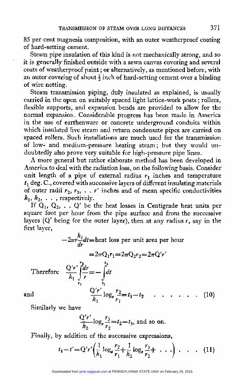
A more general but rather elaborate method has been developed in America to deal with the radiation loss, on the following basis. Consider unit length of a pipe of external radius rI inches and temperature tl deg. C., covered with successive layers of different insulating materials of outer radii y2, y3, . . r' inches and of mean specific conductivities A,, k2, . . , respectively.

If Q1, Qz, . . Q' be the heat losses in Centigrade heat units per square foot per hour from the pipe surface and from the successive layers (Q' being for the outer layer), then at any radius Y , say in the first layer,

-2mLdt=heat loss per unit area per hour k dr

Q ' r t Therefore - -=- kl

and

Similarly we have Q'r' -log, 3=t2-t3, and so on. kZ 72

Finally, by addition of the successive expressions,

(11) 1 72 1 r3

tl-t'=Q'r' - log,-+- log,-+ . . .) . . . (kl yl k, 72




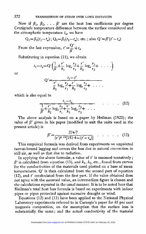
Now if pl, 192, . . . /3’ are the heat loss coefficients per degree Centigrade temperature difference between the surface considered and the atmospheric temperature t,, we have

Q l = p l ( t l - t , ) ; Q 2 = P 2 ( t 2 - t a ) ; etc.; also Q’=/3’(t‘-ta)

Q’ B‘ From the last expression, t’=- +t,

Substituting in equation ( l l ) , we obtain t , - tu=Q’(g,+G 1 r‘ log, r2 -+- I‘ log, Y --?+ . . . .)

rl kz r2 or

t , - t ’ Q‘= Y‘ r2 r’ r - log,-+-log,-1+ . . . k l Y l A 2 y2

which is also equal to

(12) . . , . t l - - ta

-+-log,-+-log,-+ 1 Y‘ r2 Y‘ y3 . . . B’ A1 rl k2 y2

The above analysis is based on a paper by Heilman (1922); the value of p’ given in his paper (modified to suit the units used in the present article) is

This empirical formula was derived from experiments on unpainted canvas-bound lagging and covers the loss due to natural convection in still air, as well as that due to radiation.

In applying the above formula, a value of t‘ is assumed tentatively; p’ is calculated from equation (13), and k,, K 2 , etc., found from curves for the conductivities of the materials used plotted on a base of mean temperatures. Q‘ is then calculated from the second part of equation (12), and t’ recalculated from the first part. If the value obtained does not agree with the assumed value, an intermediate figure is chosen and the calculations repeated in the usual manner. It is to be noted here that Heilman’s total heat loss formula is based on experiments with indoor pipes or pipes protected against excessive draught or wind.

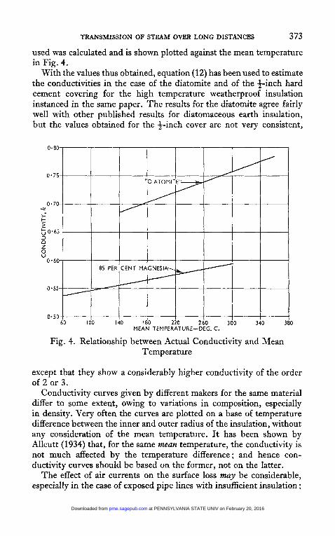
Equations (12) and (13) have been applied to the National Physical Laboratory experiments referred to in Carnegie’s paper for 85 per cent magnesia composition, on the assumption that the surface loss is substantially the same ; and the actual conductivity of the material




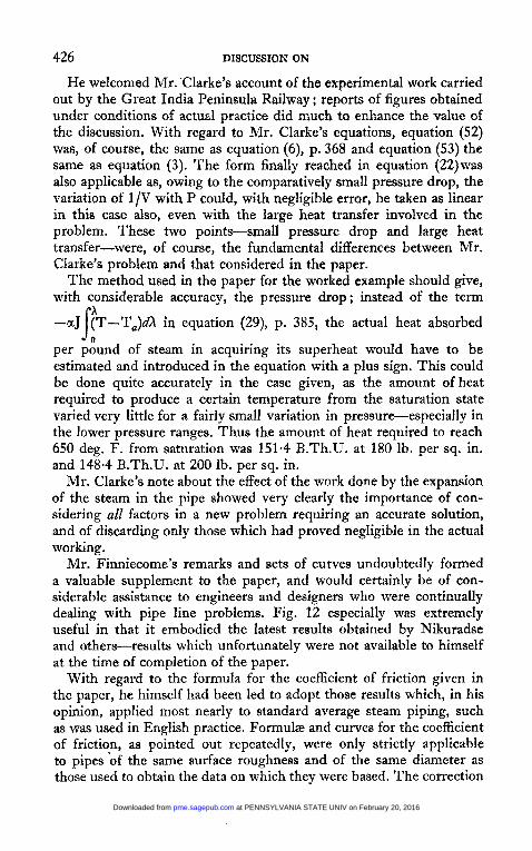
used was calculated and is shown plotted against the mean temperature in Fig. 4.

With the values thus obtained, equation (12) has been used to estimate the conductivities in the case of the diatomite and of the $-inch hard cement covering for the high temperature weatherproof insulation instanced in the same paper. The results for the diatomite agree fairly well with other published results for diatomaceous earth insulation, but the values obtained for the &inch cover are not very consistent,

Fig. 4. Relationship between Actual Conductivity and Mean Temperature

except that they show a considerably higher conductivity of the order of 2 or 3.

Conductivity curves given by different makers for the same material differ to some extent, owing to variations in composition, especially in density. Very often the curves are plotted on a base of temperature difference between the inner and outer radius of the insulation, without any consideration of the mean temperature. It has been shown by Allcutt (1934) that, for the same mean temperature, the conductivity is not much affected by the temperature difference ; and hence conductivity curves should be based on the former, not on the latter.

The effect of air currents on the surface loss may be considerable, especially in the case of exposed pipe lines with insufficient insulation ;




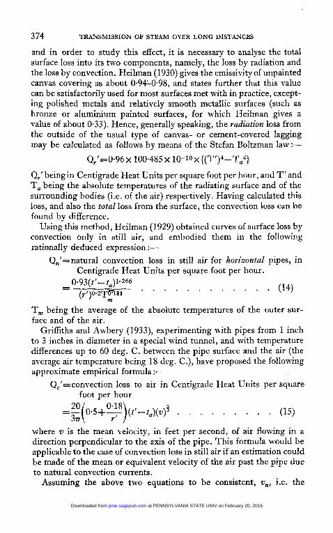
and in order to study this effect, it is necessary to analyse the total surface loss into its two components, namely, the loss by radiation and the loss by convection. Heilman (1930) gives the emissivity of unpainted canvas covering as about 0.960.98, and states further that this value can be satisfactorily used for most surfaces met with in practice, except- ing polished metals and relatively smooth metallic surfaces (such as bronze or aluminium painted surfaces, for which Heilman gives a value of about 0.33). Hence, generally speaking, the radiation loss from the outside of the usual type of canvas- or cement-covered lagging may be calculated as follows by means of the Stefan Boltzman law :-

Q,’=0*96~ 100.485 x ~O-’”X{(T’)~-T,~}

0,’ being in Centigrade Heat Units per square foot per hour, and T’ and T, being the absolute temperatures of the radiating surface and of the surrounding bodies (i.e. of the air) respectively. Having calculated this loss, and also the total loss from the surface, the convection loss can be found by difference.

Using this method, Heilman (1929) obtained curves of surface loss by convection only in still air, and embodied them in the following rationally deduced expression :-

Qn’=natural convection loss in still air for horizontal pipes, in Centigrade Heat Units per square foot per hour.

(14) - ( , l)o.2T~181 . * . . . * . . - - 0*93( t ’ - tJ1.266

m

T, being the average of the absolute temperatures of the outer surface and of the air.

Griffiths and Awbery (1933), experimenting with pipes from 1 inch to 3 inches in diameter in a special wind tunnel, and with temperature differences up to 60 deg. C. between the pipe surface and the air (the average air temperature being 18 deg. C. ) , have proposed the following approximate empirical formula :-

Qc’=convection loss to air in Centigrade Heat Units per square foot per hour

=- 20 ( 0 * 5 + 7 ) ( t ’ - t ~ ( ~ ) ~ . . . . . . . . . 31r

where v is the mean velocity, in feet per second, of air flowing in a direction perpendicular to the axis of the pipe. This formula would be applicable to the case of convection loss in still air if an estimation could be made of the mean or equivalent velocity of the air past the pipe due to natural convection currents.

Assuming the above two equations to be consistent, v,,, i.e. the



TRANSMISSION OF STEAM OVER LONG DISTANCES * 375

equivalent velocity for natural convection, can be foupd by equating Q,’ and Qn‘. This gives

(t’- tu)0.266 o>= ?! x 0.93 x 2o (r’)O*2(0~5+-)Tm 0.18 0.181

Y’

Now in this expression the term (r’)O-2 ( 0*5+- ,,,) varies very little

for values of Y’ from 4 inch to 6 inches (i.e. for pipe diameters of 1 inch to 12 inches), a fair average value being about 0.7. Also, in a series of calculations on the high-temperature insulation referred to earlier, it was found that for a change in steam temperature from 177 deg. C. to 344 deg. C., the change in the temperature t‘ of the outer surface was only about 24 deg. C., the air temperature being 21 deg. C. Assuming therefore the average value of t’ in those calculations (which was about

55 deg. C.) we can, without much error, take Tm=273+*5=311

deg. C. absolute. Substituting these two values, we obtain the following approximate

relationship :-

2

3 3nx 0.93 (t’-tu)”*266 vn =- X 20 0*7~3110.181

from which ~,=0.1043(t’--t,)0*4 . . . . . (16) Griffiths and Awbery’s equation, [i.e. equation (15)] will therefore

give nearly the same results as Heilman’s for a value of v equal to v, calculated from equation (16).

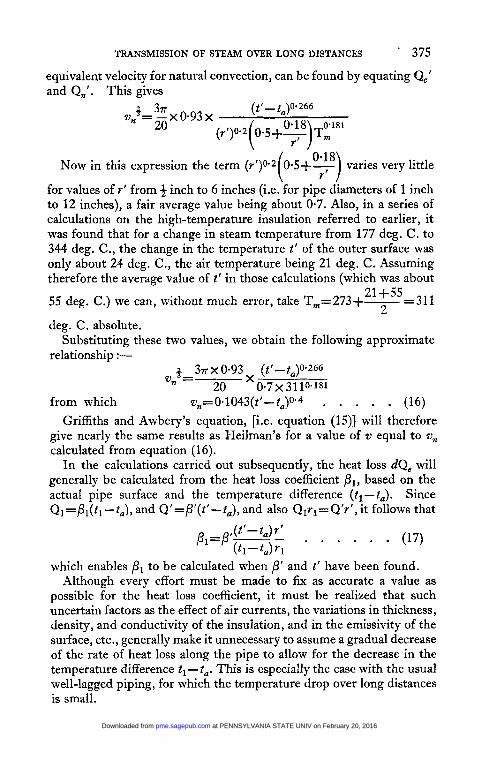
In the calculations carried out subsequently, the heat loss dQ, will generally be calculated from the heat loss coefficient /I1, based on the actual pipe surface and the temperature difference ( t l - tu) . Since Q1=/I l ( t l - tu) , and Q’=p’(t’-t,), and also Q1rl=Q’r’, it follows that

which enables pl to be calculated when p’ and t’ have been found. Although every effort must be made to fix as accurate a value as

possible for the heat loss coefficient, it must be realized that such uncertain factors as the effect of air currents, the variations in thickness, density, and conductivity of the insulation, and in the emissivity of the surface, etc., generally make it unnecessary to assume a gradual decrease of the rate of heat loss along the pipe to allow for the decrease in the temperature difference t l- tu. This is especially the case with the usual well-lagged piping, for which the temperature drop over long distances is small.




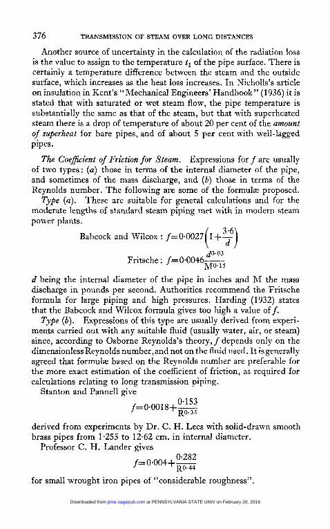
Another source of uncertainty in the calculation of the radiation loss is the value to assign to the temperature t , of the pipe surface. There is certainly a temperature difference between the steam and the outside surface, which increases as the heat loss increases. In Nicholls’s article on insulation in Kent’s “Mechanical Engineers’ Handbook” (1936) it is stated that with saturated or wet steam flow, the pipe temperature is substantially the same as that of the steam, but that with superheated steam there is a drop of temperature of about 20 per cent of the amount of superheat for bare pipes, and of about 5 per cent with well-lagged pipes.

Expressions for f are usually of two types: (u) those in terms of the internal diameter of the pipe, and sometimes of the mass discharge, and (b) those in terms of the Reynolds number. The following are some of the formula3 proposed.

Type ( a ) . These are suitable for general calculations and for the moderate lengths of standard steam piping met with in modern steam power plants.

The Coefficient of Friction for Steam.

Babcock and Wilcox : f=0*0027 1 +- ( 3:) d0.03

Fritsche : f=0*0046m5

d being the internal diameter of the pipe in inches and M the mass discharge in pounds per second. Authorities recommend the Fritsche formula for large piping and high pressures. Harding (1 932) states that the Babcock and Wilcox formula gives too high a value off.

Expressions of this type are usually derived from experiments carried out with any suitable fluid (usually water, air, or steam) since, according to Osborne Reynolds’s theory, j depends only on the dimensionless Reynolds number,and not on the fluid used. It is generally agreed that formulE based on the Reynolds number are preferable for the more exact estimation of the coefficient of friction, as required for calculations relating to long transmission piping.

Type (b).

Stanton and Pannell give - 0.153 f= 0.001 8 +- RO- 3 5

derived from experiments by Dr. C . H. Lees with solid-drawn smooth brass pipes from 1.255 to 12.62 cm. in internal diameter.

Professor C . H. Lander gives

for small wrought iron pipes of “considerable roughness”.




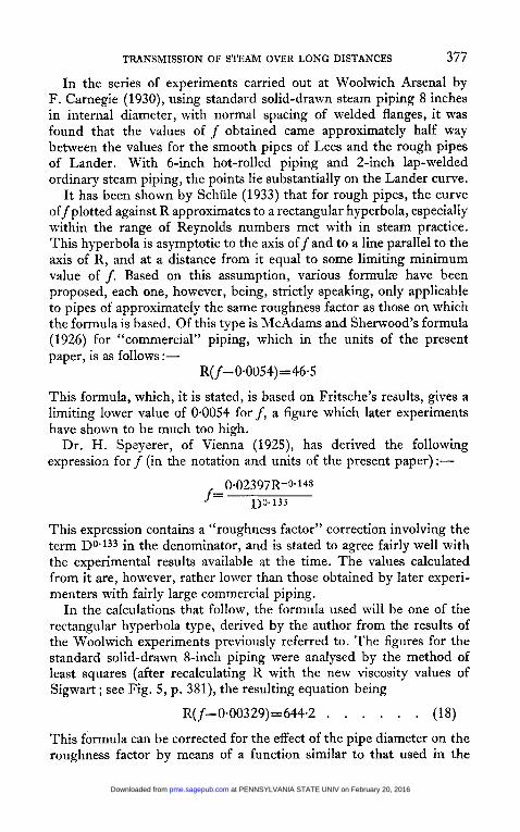
In the series of experiments carried out at Woolwich Arsenal by F. Carnegie (1930), using standard solid-drawn steam piping 8 inches in internal diameter, with normal spacing of welded flanges, it was found that the values of f obtained came approximately half way between the values for the smooth pipes of Lees and the rough pipes of Lander. With 6-inch hot-rolled piping and 2-inch lap-welded ordinary steam piping, the points lie substantially on the Lander curve.

It has been shown by Schule (1933) that for rough pipes, the curve offplotted against R approximates to a rectangular hyperbola, especially within the range of Reynolds numbers met with in steam practice. This hyperbola is asymptotic to the axis off and to a line parallel to the axis of R, and at a distance from it equal to some limiting minimum value o f f . Based on this assumption, various formulae have been proposed, each one, however, being, strictly speaking, only applicable to pipes of approximately the same roughness factor as those on which the formula is based. Of this type is McAdams and Shenvood’s formula (1926) for “commercial” piping, which in the units of the present paper, is as follows :-

This formula, which, it is stated, is based on Fritsche’s results, gives a limiting lower value of 0.0054 for f , a figure which later experiments have shown to be much too high.

Dr. H. Speyerer, of Vienna (1925), has derived the following expression for f (in the notation and units of the present paper):-

R(f- 0.0054)= 46.5

0-02397R-0.148 f= D0.133

This expression contains a “roughness factor” correction involving the term DO-133 in the denominator, and is stated to agree fairly well with the experimental results available at the time. The values calculated from it are, however, rather lower than those obtained by later experi- menters with fairly large commercial piping.

In the caIcuIations that follow, the formula used will be one of the rectangular hyperbola type, derived by the author from the results of the Woolwich experiments previously referred to. The figures for the standard solid-drawn 8-inch piping were analysed by the method of least squares (after recalculating R with the new viscosity values of Sigwart ; see Fig. 5 , p. 381), the resulting equation being

R(f-0*00329)=644*2 . . . . . . (18)

This formula can be corrected for the effect of the pipe diameter on the roughness factor by means of a function similar to that used in the




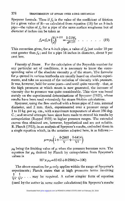
Speyerer formula. Thus if f 8 is the value of the coefficient of friction for a given value of R-as calculated from equation (18) for an 8-inch pipe-the value of fd for a pipe of the same surface roughness but of diameter d inches can be taken as

This correction gives, for a 4-inch pipe, a value of f d just under 10 per cent greater than f 8 ; and for a pipe 16 inches in diameter, about 9 per cent less.

Viscosity of Steam. For the calculation of the Reynolds number for any particular set of conditions, it is necessary to know the corresponding value of the absolute viscosity p of the steam. The formuh for p quoted in various textbooks are usually based on obsolete experiments, and take no account of the variation of viscosity with pressure. It was, however, held for some years-and until quite recently-that, at the high pressures at which steam is now generated, the increase of viscosity due to pressure was quite considerable. This view was based mainly on the experimental determinations of Speyerer (1925), whose results have been used extensively for steam friction calculations.

Speyerer, using the flow method with a brass pipe of 2 mm. internal diameter, and 2 mm. thick, experimented over a pressure range of 1 to 10 kg. per sq. cm., with a maximum temperature of about 350 deg. C. ; and several attempts have since been made to extend his results by extrapolation (Ruppel 1935) to higher pressure ranges. The extended curves thus obtained are, however, hypothetical and are not reliable. R. Planck (1933), in an analysis of Speyerer’s results, embodied them in a single equation which, in the notation adopted here, is as follows :-

( 0,2803 0.6414) +- V2 p=po I+- V

po being the limiting value of p when the pressure becomes zero. The equation for po derived by Planck by extrapolation from Speyerer’s values is

l O 7 ~ po= 83*02+0*2506(t- 100)

The above equation for p only applies within the range of Speyerer’s experiments ; Planck states that at high pressures terms involving

. may be required. A rather simpler form of equation 1 1

(used by the author in some earlier calculations) fits Speyerer’s results v3’ V4’ * .




with approximately the same accuracy-and with the same limitations -as Planck’s equation. It is

(p/po- 1.007)V1*6*5= 1

the values of p,, being as calculated from PIanck’s expression. Later experimental work, mainly by Sigwart (1936), gives results

which show considerable disagreements with Speyerer’s figures and Planck’s analysis. Sigwart used capillaries of quartz and of platinum- about 35 cm. long, and 0.389 and 0.548 mm. internal diameter respectively-andvery sensitive apparatus for the measurement of the pressure drop ; and his results appear to be the most reliable up to date. He states that they agree with those of Schugajew (1934) in so far as they show no appreciable effect of pressure on viscosity below a temperature of about 275 deg. C. ; within this limit, they practically agree with the values obtained from Sutheriand’s well-known formula

C

I*=p (at 0 deg. C.) x -

With c=548 and p from Speyerer’s equation for a pressure of 1 kg. per sq. cm.,

deg. ~--)=60*81 x 10-7, and also with those values

l o 7 x p= 84-36+0.2496(t-100)

Above 275 deg. C., the average increase in viscosity for a series of isothermals (up to 383 deg. C.) was found to be of the order of 5 per cent for an increase of pressure from 1 to 100 kg. per sq. cm.

Sigwart states that Speyerer’s results are about 9 per cent too high because he neglected to make certain corrections (mainly for the kinetic energy of the fluid at outlet) in his pressure drop measurements, and also because his brass capillary tube was strained beyond the elastic limit before his measurements were made.

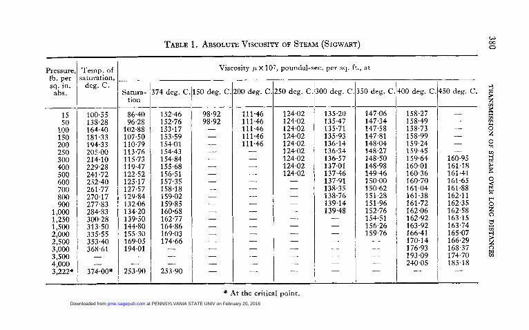
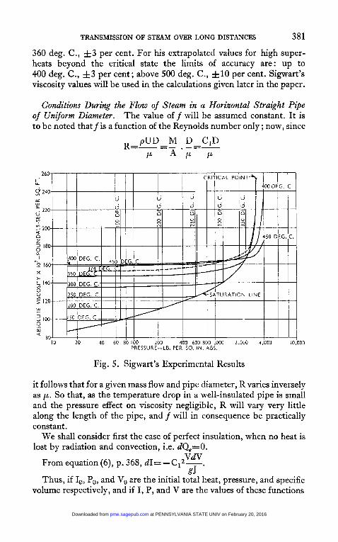
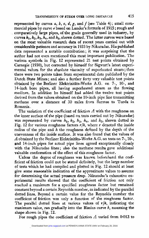
Sigwart’s experiments on steam were carried out over a range of pressures from 25 to 270 kg. per sq. cm. and of temperatures from 276.3 deg. C. to 382.7 deg. C. ; his final tabulated results, recalculated in English units, are shown plotted in Fig. 5 on a base of logarithms of absolute pressures in pounds per square inch, and are also given in Table 1. His extrapolated figures for the region beyond the range of his experiments have been in some cases slightly altered, as it was found that, when plotted on a pressure base, they did not lie on a smooth curve. Sigwart estimates the accuracy of his experimental results to be within the following limits: up to 360 deg. C., f 2 per cent; above



Pressure lb. per sq. in.

abs.

158.27 158.49 158.73 158.99 159.24 159.45 159.64 160.01 160.36 160.70 161.04 161-38 161-72

15 50

100 150 200 250 300 400 500 600 700 800 900

1,000 1,250 1,500 2,000 2,500 3,000 3,500 4,000 3,222"

- - - - - -

160.95 161.18 161.41 161.65 161.88 162.11 162.35

Temp: of mturation, deg. C.

162.06 162.92 163.92 166.41 170.14 176.93 193.09 240.05

100.55 138.28 164.40 181.33 194.33 205.00 214.10 229.28 241.72 252.40 261.77 270.17 277.83 284.83 300.28 313.50 335.55 353.40 368.61 - -

374.00'

162.58 163.15 163.74 165.07 166.29 168.37 174.70 185.18

TABLE 1. ABSOLUTE VISCOSITY OF STEAM (SIGWART)

Satura- tion

86.40 96.28

102.88 107.50 110.79 113.76 115.73 11 9.47 122.52 125.17 127.57 129.84 132.06 134.20 13950 144.80 155.30 169.05 194.01 - -

253.90 -

Viscosity p x 107, poundal-sec. per sq. ft., at

74 deg. C

152.46 152.76 153.17 153.59 154.01 154.43 154.84 155.68 156.51 157.35 158.18 159.02 159.85 160.68 162.77 164.86 169.03 174.66 - - -

253.90

!SO deg. C

124.02 124.02 124.02 124.02 124.02 124.02 124.02 124.02 124.02 - - - - - - - - - - - - -

00 deg. C

135.20 135.47 135.71 135.93 136.14 136.34 136.57 137.01 137.46 137.91 138.35 138.76 139.14 139.48 - - - - - - - -

50 deg. C

147.06 147.34 147.58 147.81 148.04 148.27 148.50 148.98 149.46 150.00 150.62 151.28 151.96 152.76 154.51 156.26 159.76 - - - - -

.OO deg. C.450 deg. C. i

* At the critical point. at PENNSYLVANIA STATE UNIV on February 20, 2016pme.sagepub.comDownloaded from



360 deg. C., f 3 per cent. For his extrapolated values for high superheats beyond the critical state the limits of accuracy are: up to 400 deg. C., f3 per cent ; above 500 deg. C., f10 per cent. Sigwart’s viscosity values will be used in the calculations given later in the paper.

Conditions During the Flow of Steam in a Horizontal Straight Pipe of Uniform Diameter. The value off will be assumed constant. It is to be noted thatfis a function of the Reynolds number only ; now, since

pUD M D - C,D R=-=- F A - F P

Fig. 5. Sigwart’s Experimental Results

it follows that for a given mass flow and pipe diameter, R varies inversely as p. So that, as the temperature drop in a well-insulated pipe is small and the pressure effect on viscosity negligible, R will vary very little along the length of the pipe, and f will in consequence be practically constant.

We shall consider first the case of perfect insulation, when no heat is lost by radiation and convection, i.e. dQ,=O.

VdV From equation (6), p. 368, dI=-C,z-.

Thus, if I,, Po, and Vo are the initial total heat, pressure, and specific volume respectively, and if I, P, and V are the values of these functions

gJ




after passing a length X of the pipe, we have, by integration, C 2

I ~ - - I = ~ ( V ~ - V , ~ ) . . . . . 2gJ

V P

From equation (8), p. 369,

so that

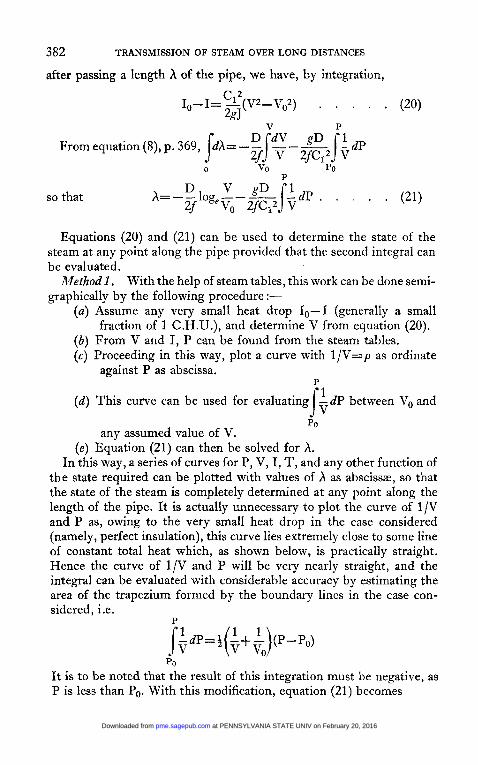
Equations (20) and (21) can be used to determine the state of the steam at any point along the pipe provided that the second integral can be evaluated.

Method 1. With the help of steam tables, this work can be done semi- graphically by the following procedure :-

(u) Assume any very small heat drop &--I (generally a small

( b ) From V and I , P can be found from the steam tables. (c ) Proceeding in this way, plot a curve with l /V=p as ordinate

fraction of 1 C.H.U.), and determine V from equation (20).

against P as abscissa.

(d ) This curve can be used for evaluating -dP between Vo and PO J;

any assumed value of V. (e) Equation (21) can then be solved for A.

In this way, a series of curves for P, V, I, T, and any other function of the state required can be plotted with values of h as abscissae, so that the state of the steam is completely determined at any point along the length of the pipe. It is actually unnecessary to plot the curve of l / V and P as, owing to the very small heat drop in the case considered (namely, perfect insulation), this curve lies extremely close to some line of constant total heat which, as shown below, is practically straight. Hence the curve of 1/V and P will be very nearly straight, and the integral can be evaluated with considerable accuracy by estimating the area of the trapezium formed by the boundary lines in the case considered, i.e.

P

-a=* -+- (P-P,) PO s: (i ;J

It is to be noted that the result of this integration must be negative, as P is less than Po. With this modification, equation (21) becomes




A=-- log, -+- -+- (P-Po) . . (22) ;[ ; 2&(: :o) ] T o show that the lines of constant total heat on a diagram relating 1/V and P are nearly straight lines passing through the origin, Callendar's equation for the total heat I can be used. This equation is of the form

13 bP 13 lob I- B =-P(V-b)+ - = -PV- -p 35 J 35 35

The constants as given in the 1931 Revised Tables are : b= -0.00280 cu. ft. per lb.; B=464 C.H.U. per lb. Substituting these, we obtain

13 1=464+-PV+O*O0933P C.H.U. per Ib. 35

For constant total heat I, dI=O, i.e. 13d(PV)=-0*0280dP s o Pv=-o~oo2154P+c

P - 1 v-'= C - 0.0021 54P and

The term -0.002154P is always very small compared with C ; thus the value of C at a pressure of 2,000 lb. per sq. in. abs. and temperature 460 deg.. C . is 99,116, whilst the value of 0*002154P is only 620, i.e. 0.625 per cent. At low pressures the correction is quite negligible. Hence p varies directly as P for constant total heat.

Using Callendar's equation for the total heat, the author has obtained, by means of a slight modification, a direct mathematical

evaluation of the integral /$P.

Method 2.

P

PO 13 0.0093 3dp dI=-d(PV)+ - 3J J

VdV RJ

We have

= -C,2-, by equation (6)

c2

J -const.=-, say. C12V2 13- 0.00933P +-PV+-- Hence, by integration, - J 2gJ 3J

Therefore

and

C12V2 13 c2= -+ -PV+O.O0933P 2g 3

21: 3 -- - c12v02+~PoVo+O*O0933P~ . . (23)

C,WZ c,-- 2g . . . . . . p=,,

'3V+0*00933 3




The denominator of this expression will not be greatly affected by neglecting the constant 0.00933. Thus with V=0*342 cu. ft. per lb. (corresponding to steam at rest at 2,000 lb. per sq. in. abs. and 460 deg. C.), the effect of neglecting this term is to increase the calculated pressure by about 0.6 per cent.

Neglecting this term, and differentiating with respect to V, we get

dP 3C12 dV 3c2 dV Therefore -=--. ---.- V 26g V 13 V3

Substituting this in equation (21), we finally obtain

-23loge- "1 . . . . (25) VO

The problem can then be solved entirely from equations (23) and (25).

Method 3. From equations (23) and (24),

13 - C"(V2- VOZ) + Po(V- V,) . . . (26) 2.e

13 -V+0.00933 3

P-Po=

This can be calculated for an assumed value of V, and A then found directly from equation (22).

Of the solutions given above, method 1 will give the same results as method 3 provided the Callendar Revised Tables (1931) are used. Method 1 can, however, be used with any other standard tables. Method 2 will give quite accurate results for pressures up to about 1,500 lb. per sq. in., but method 3 should be rather more accurate over the whole range of pressures.

Correction for the Radiation Loss.- The radiation loss dQ, is included in equation (6) :-

dI = - y V d V + dQ, gJ

If denotes the heat loss coefficient from the outside of the pipe



TRANSMISSION OF STEAM OVER LONG DISTANCES 3 85

(of diameter D1), then for a length dh, the loss per pound of flow with a temperaturc drop from T to the atmospheric temperature T,

Neglecting the variations in 81 as the temperature drops along the pipe, then u is a constant for the pipe with the assumed mass flow M. We have therefore

c 2vdv dI= -1 -a(T--T,)dA

gJ 13 0.00933 3T J

This is also equal to -d(PV)+-dP as before.

Therefore x

. . (28) 0.00933P Cz (T-T,)~A+~(PV)+ --- - 35 J J

0

The second term vanishes when X=O.

Thus, as before, C 2 = ~ V o ~ + ~ P o V o + O ~ O 0 9 3 3 P ~ (equation 23) 2g

c12v2 aJ (T-TJdX

and P= . . . . . (29) J) c2- -- 0

2s

13 -V+ 0.00933 3

It is sufficient, at least for a first approximation, to assume (T-T,) constant and equal to (To-TJ, so that the radiation loss can be taken equal to aJ(To-T,)X.

Points for the condition curves along the length of the pipe are obtained by trial and error, the method of procedure being as follows :-

(a) First calculate h, for a chosen value of V, assuming no heat loss, by equation (25) or by method 3 given above.

(b) Estimate the heat loss aJ(To-T,)X. (c) Assuming V unchanged, recalculate P by equation (29). (d) Recalculate h by equation (22), not equation (25). (e) Find the end temperature T from the steam tables.

To+T (f) Check the heat loss, using the mean temperature - 2

(g) Make a second approximation if necessary. instead of To.

The method of correction given above is also based on the assump- 26




tion of a straight-line relationship between 1/V and P, even with the radiation loss. With well-lagged pipes, this assumption is within the limits of accuracy of the fixed values adopted for the temperature difference, for the heat loss coefficient PI, and for the coefficient of frictionf; and the method can be used for pipes of considerable length.

In practice, for very long pipes, it may be advisable in certain cases to carry out the calculations in a series of definite steps, e.g. for successive lengths of not more than 2,000 feet. Where the radiation loss is

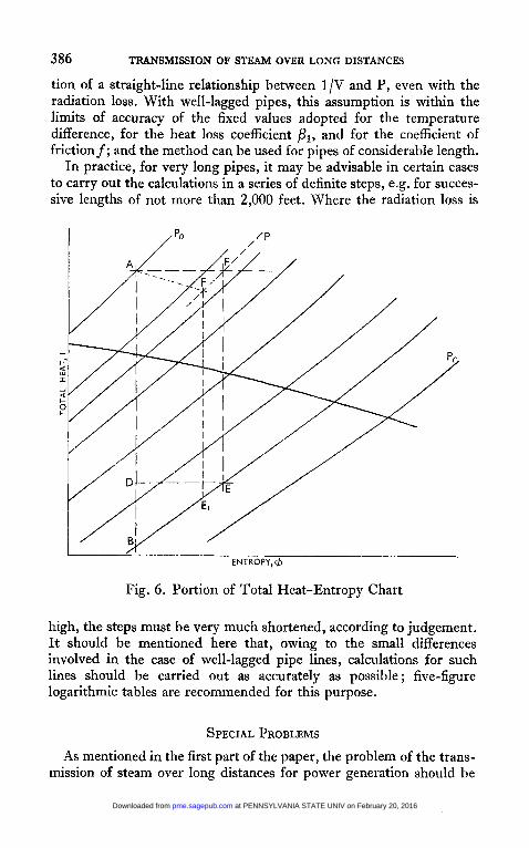
Fig. 6. Portion of Total Heat-Entropy Chart

high, the steps must be very much shortened, according to judgement. It should be mentioned here that, owing to the small differences involved in the case of well-lagged pipe lines, calculations for such lines should be carried out as accurately as possible; five-figure logarithmic tables are recommended for this purpose.

SPECIAL PROBLEMS As mentioned in the first part of the paper, the problem of the trans-

mission of steam over long distances for power generation should be




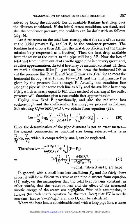
solved by fixing the allowable loss of available Rankine heat drop over the distance considered. If the initial steam conditions are fixed, and also the condenser pressure, the problem can be dealt with as follows (Fig. 6).

Let A represent on the total heat-entropy chart the state of the steam at the initial pressure Po, and let P, be the condenser pressure. The Rankine heat drop is then AB. Let the heat drop efficiency of the transmission be y (expressed as a fraction). Then the heat drop available from the steam at the outlet to the pipe will be y.AB. Now the loss of total heat from inlet to outlet of a well-lagged pipe is not very great ;and, as a first approximation, the total heat may be assumed constant. If, then, we mark a distance BD=(l-y)AB on BA, draw the horizontal DE to cut the pressure line P, at E, and from E draw a vertical line to meet the horizontal through A at F, then FE=y.AB, and the final pressure P is given by the pressure line through F. Actually, the condition line along the pipe will be some such line as AF,, and the available heat drop FIE1, which is nearly equal to FE. This method of arriving at the outlet pressure will therefore give a reasonable first approximation.

Having now fixed P provisionally, and also the radiation loss coefficient B1 and the coefficient of friction f, we proceed as follows. Substituting C12= 16Mz/&D4, we obtain from equation (22),

Since the determination of the pipe diameter is not an exact matter- the nearest commercial or practical size being selected-the term - D V - log, -, which is comparatively small, can be neglected. 2f vo

or

=const., when X and P are fixed. In general, with a small heat Ioss coefficient bl, and for fairly short

pipes, it will be sufficient to arrive at the pipe diameter from equation (31) only, on the assumption that the total heat remains constant, in other words, that the radiation loss and the effect of the increased kinetic energy of the steam are negligible. With this assumption, it follows (by Callendar's equation for the total heat) that PV is nearly constant. Hence V=PoVo/P, and also D, can be calculated.

Where the heat loss is considerable, and with a long pipe line, a more




accurate solution can be obtained by taking account of this loss in the following manner. From equations (27) and (28),

C C 2V2 13PV 0.00933P Q!Q~=-~-L-- - ~ 1 J %J 3J J 0

This is also equal to B1aDIA(To-rrT,), on the assumption that (To-Ta) 3,600M

is nearly constant. From this we have, after substitution for C2 and C1,

/317~D lA(T0- To)- 8M2(Vo2-V2) 1 ~(PoVO-PV) 4- 3J

- - 3,600M AYgJ

( 3 4 O*OO933(Po-P) . . . .

J + The procedure is now as follows. By means of equation (31), con-

verted to logarithmic form, D is calculated for a number of increasing values of V. Then, using corresponding values of D and V, calculate :-

. . . . . . . . . . . Pl~D,W*---T,) Y,= 3,600M (33)

* (34) 8M2(Vo2 - V2) 1 3(PoV0- PV) 0.0093 3 (Po- P)

J + i- 3J and Y,=

v2D4gJ Plot Y1 and Y2 against D as abscissa; the value of D at the point of

intersection of the two curves is the value required. The nearest practical or commercial size should then be selected. It should be noted that since D,=D+28 (8 being the thickness of the pipe), some reasonable value of this thickness should be assumed ; any small error in this assumption is of little importance.

Typical Worked ExamJle. The following problem will now be worked out completely: Given P0=1,200 lb. per sq. in. abs.; to =360 deg. C.; ta=15 deg. C.; M=30 lb. per sec.; A=5,000 feet; condenser pressure Pc=0*5 Ih. per sq. in. abs., it is required to find a suitable pipe diameter for a heat drop efficiency of 95 per cent in the transmission, and then to calculate as exactly as possible the actual final state of the steam for the pipe selected.

From the Callendar total heat-entropy chart, 10=723 C.H.U. per lb. After adiabatic expansion to 0.5 lb. per sq. in. abs., the total heat is 442 C.H.U. lb. The Rankine or adiabatic heat drop is thus 281 C.H.U. per Ib. A loss of 5 per cent of this amount is about 14 C.H.U. per lb. ; so on the assumption of constant total heat during the Aow, as explained



TRANSMISSION OF STJUM OYER LONG DISTANCES 389

before, the total heat after adiabatic expansion from the outlet pressure to the condenser pressure should be about 456 C.H.U. per Ib. The construction outlined above gives an outlet pressure of 760 lb. per sq. in. abs. approximately ; and this value will be assumed provisionally.

From Callendar's (1931) steam tables, V0=0.482 cu. ft. per lb. We assume further, at the outset, that j=0-0035, and that the heat loss coefficient &=0.3 C.H.U. per sq. ft. per hour per deg. C. temperature difference. With these figures, we have from equation (31),

DS(L+L) = 6 4 ~ 3 0 2 ~ 0 . 0 0 3 5 ~ 5,000 V 0.482 $X 32.2(1,200-760)~ 144

from which we get

If the total heat of the steam remained constant during flow, the product PV would also be nearly constant, i.e. for a pressure of 760 lb.

per sq. in. abs. the final specific volume would be about LX 0-482

=0-761 cu. ft. per Ib. Actually, since there is a reduction in the total heat, the final specific volume will be less than this; and it will not therefore be necessary to consider values of V greater than, say, 0.75 cu. ft. per Ib. We have then, from equations (33) and (34), assuming a thickness of 0.5 inch (=0.08 foot) for the pipe,

1 200 760

0~3~(D+0~08)~5,000~(360-15) Y,= 3,600 x 30

from which log Y, = 1.17764+10g (D +0.08)

8 x 30*(V2-0.4822) 13 x 144(1,200~ 0.482-760V) 3 x 1,400 Y,=- +

T ~ X 32.2 x 1,400D4 0.00933 x 144 x 440

-f- 1,400

It is to be noted that the first term in the expression for Y, is negligible at high pressures but not at low pressures ; the reverse is the case for the third term.

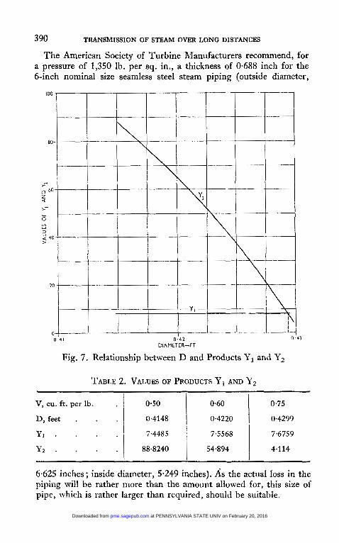
Table 2 shows the results of the calculations for three assumed values of V. The curves of Y, and Y, plotted against D are shown in Fig. 7; the value of D at the point of intersection is 0.429 foot (5.15 inches).




The American Society of Turbine Manufacturers recommend, for a pressure of 1,350 lb. per sq. in., a thickness of 0.688 inch for the 6-inch nominal size seamless steel steam piping (outside diameter,

V, cu. ft. per lb.

D, feet . Y1 . Y2 .

Fig. 7. Relationship between D and Products Y, and Y,

TABLE 2. VALUES OF PRODUCTS Y, AND Y,

0.50 0.60 0.75

0.4148 0.4220 0.4299

7-4485 7.5568 7.6759

88.8240 54.894 4.114



TRANSMISSION OF STEAM OVER LONG DISTANCES

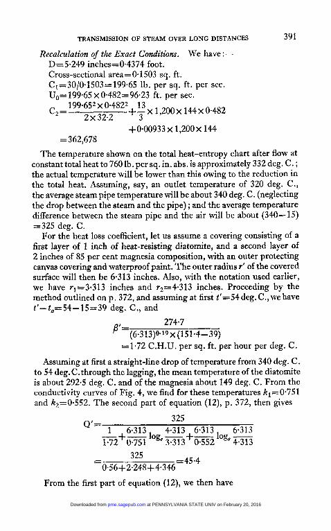
Recalculation of the Exact Conditions. D=5.249 inches=0*4374 foot. Cross-sectional area=0*1503 sq. ft. C1=30/0.1503=199*65 lb. per sq. ft. per set. Uo= 199-65 x 0-482=96-23 ft. per sec.

We have :-

199-652 x 0,4822 + 7 ~ 1 , 2 0 0 ~ 1 4 4 ~ 0 - 4 8 2 13 C2 = 2 x 32.2

+0*00933 x 1,200x 144 =362,678

391

The temperature shown on the total heat-entropy chart after flow at constant total heat to 760 Ib. per sq. in. abs. is approximately 332 deg. C. ; the actual temperature will be lower than this owing to the reduction in the total heat. Assuming, say, an outlet temperature of 320 deg. C., the average steam pipe temperature will be about 340 deg. C. (neglecting the drop between the steam and the pipe) ; and the average temperature difference between the steam pipe and the air will be about (340-15) =325 deg. C.

For the heat loss coefficient, let us assume a covering consisting of a first layer of 1 inch of heat-resisting diatomite, and a second layer of 2 inches of 85 per cent magnesia composition, with an outer protecting canvas covering and waterproof paint. The outer radius rt of the covered surface will then be 6.313 inches. Also, with the notation used earlier, we have ~ ~ e 3 . 3 1 3 inches and r2=4-313 inches. Proceeding by the method outlined on p. 372, and assuming at first t’=54deg. C., we have t’-t,=54-15=39 deg. C., and

274.7 ”=(6.33)0.19 x (1 51-4-39)

11.72 C.H.U. per sq. ft. per hour per deg. C.

Assuming at first a straight-line drop of temperature from 340 deg. C. to 54 deg. C.through the lagging, the mean temperature of the diatomite is about 292.5 deg. C. and of the magnesia about 149 deg. C. From the conductivity curves of Fig. 4, we find for these temperatures k,=0.751 and k,=0.552. The second part of equation (12), p. 372, then gives

325 1 6.313 4.313 6.313 6.313

1.72 0.751 3.313 0.552 4 313

Q’=

- + - log, - +- log, -

=45*4 325 0-56+ 2*248+ 4.346

- -

From the first part of equation (12), we then have




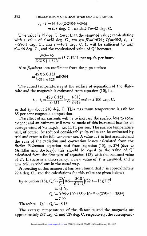
ti - t' = 45.4 x (2*248+4.346) =298 deg. C. , so that t'=42 deg. C .

This value is 12 deg. C. lower than the assumed value : recalculating with a value of t'=48 deg. C., we get /3'=1*634; Q'=45.2, tl-t' =296.3 deg. C., and t'=43.7 deg. C . It will be sufficient to take t'=46 deg. C., and the recalculated value of Q' becomes

340-46 =45 C.H.U. per sq. ft. per hour. 2.248+4*346

Also &=heat loss coefficient from the pipe surface

- 4 5 . 0 ~ 6-313=0,264 - 3.313 x 325

The actual temperature t2 at the surface of separation of the diatomite and the magnesia is estimated from equation (lo), i.e.

45x 6'313 log, ?=about 100 deg. C. f , - t z = 3 313 0.75 1

so that t2=about 240 deg. C. This maximum temperature is safe for 85 per cent magnesia composition.

The effect of air currents will be to increase the surface loss to some extent ; and an estimate will now be made of this increased loss for an average wind of 7.5 m.p.h., i.e. 11 ft. per sec. The surface temperature will, of course, be reduced considerably ; its value can be estimated by trial and error in the following manner. A value of t' is first assumed and the sum of the radiation and convection losses calculated from the Stefan Boltzman equation and from equation (15), p. 374 (due to Griffiths and Awbery); this should be equal to the value of Q' calculated from the first part of equation (12) with the assumed value of t ' . If there is a discrepancy, a new value of 2' is assumed, and a new trial carried out in the usual way.

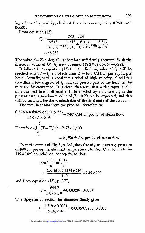
Proceeding in this manner, it has been found that t' is approximately 22.4 deg. C., and the calculations for this value are given below :-

By equation (15), Q,'= =41-04

Q,'=0.96~ 100.485 x 10-10~(29-5*4"-288") = 7.09

Therefore Q,'+ Q,'=48-13 The average temperatures of the diatomite and the magnesia are

approximately 287 deg. C. and 129 deg. C . respectively, the correspond-




ing values of k1 and k,, obtained from the curves, being 0.7503 and 0-5505.

From equation (12), 340-22.4 Q’=

6.313 4.313 6.313 6.313 0.7503 3.313 0.5505 loge 4.313 log, - + -

=48*253

The value t‘=22.4 deg. C. is therefore sufficiently accurate. With the increased value of Q’, PI now becomes (48.2/45) x 0.264=0.283.

It follows from equation (12) that the limiting value of Q’ will be reached when t‘=ta, in which case Q‘=49.3 C.H.U. per sq. ft. per hour. Actually, with a continuous wind of high velocity, t’ will fall to within a few degrees of t,, and the greater part of the heat will be removed by convection. I t is clear, therefore, that with proper insulation the heat loss coefficient is little affected by air currents; in the present case, a maximum value of P1=o*29 can be expected, and this will be assumed for the recalculation of the final state of the steam. .

The total heat loss from the pipe will therefore be

0’29X7rX 6*625x51000x 325=7.57 C.H.U. per Ib. of steam flow. 12 x 3,600 x 30

Therefore aJ (T-T,)dA=7.57 x 1,400

0 =10,596 ft.-lb. per lb. of steam flow.

J’ From the curves of Fig. 5 , p. 381, the value of p at an average pressure

of 980 lb. per sq. in. abs. and temperature 340 deg. C. is found to be 1 4 9 ~ 10-7 poundal-sec. per sq. ft., so that

- 199.65 x 0.4374~ 107,5.85 10a - 149

and from equation (18), p. 377,

6**2 + 0.00329= 0.0034 f=5-8, x 106

The Speyerer correction for diameter finally gives

f= la319 5.2490.1 0 ’0034=~*~~3597, 33 say, 0.0036




For the evaluation of the final conditions, we must now recalculate P and V from equations (22) and (29). Equation (22) gives

?+log, - V

6(1+1) P=Po-- VO

2 c p v vo and, equating the right-hand sides of this equation and of equation (29), we have

199.652V2- 2 x 0.0036 x 5,000 V 362,678- 0.43 74 3- log"O7;fx2

= 1,200 x 144- 2g

=+ 0.00933 L?- (1+2.075) 3 2 c p v

from which 352,082-61 8.95V2- - ~72,800- 82-3O4+loge 2.075V

0*0004039 -+2*075 ?+0.00933 G 1

This equation can be solved graphically by plotting the two sides against V. The curves obtained for three values of V (i.e. 0-6,0.7,0*8 cu. ft.) are shown in Fig. 8, and the value of V at the intersection is 0.71 cu. ft. per lb. The corresponding final value of P is 792 lb. per sq. in. abs. ; and the final steam temperature, as obtained from the steam tables, is 324.5 deg. C.

The adiabatic heat drops for the inlet and outlet conditions, with a condenser pressure of 0.5 lb. per sq. in. abs., have been recalculated from the steam tables, and are found to be 281-1 and 263.7 C.H.U. per lb. respectively. The actual percentage loss of available heat drop is therefore

281'1-263'7~ 100=6.19 per cent. 281.1

LIMIT VALUES IN LONG-DISTANCE TRANSMISSION OF STEAM In the fundamental equation (9), p. 369, namely

dF' C 2 2fC12 dA - + 1 = --v- d v g gD dv

the term dP/dV is negative, and is at first usually greater numerically than C,Z/g. Hence dP/dV+C12/g is at first negative and dA/dV or dV/dh is positive, that is to say, V increases along the pipe. At a certain




limiting point on the expansion (or P-V) curve, dP/dV becomes equal numerically to C12/g and then dP/dV+C12/g=O, and dAldV=O. After this point, the expression would become positive, so that dV/dA would be negative. This means that V would decrease and P would increase, so that the state point would tend to travel back along the P-V curve. Such a thing is impossible, as any compression change would be immediately followed by re-expansion to the limiting state.,

8

Hence there is a limiting point in the length of the pipe after which the specific volume and pressure cannot change unless some of the conditions originally assumed constant also change. This limiting point fixes the maximum length of pipe for the constant factors assumed initially. If the length is greater than this and the diameter is not changed, then the assumed discharge cannot be obtained, and a reduced discharge will result. At the limiting point, therefore, we have dP/dV= --C,*/g. Considering at first, as before, the case of perfect insulation, i.e. dQ,=O, then since




13 0-00933 dI=-(VdP+PdV)+-dP= 3J J

dP dv= 13V

we have also - + 0.00933

3

Ct2V’ . 13P’ - +- 13V’ -+0*00933

3

c12- g 3 Therefore -_

P’ and V’ being the limiting values of P and V.

1oc12v‘ - 13” 0 .009332 C 2 which simplifies to -_-- 3g 3 g

Substituting C1=U/V=U’/V’, by equation ( S ) , p. 368, we obtain finally

If the small term O.O02799/V‘ in the denominator is neglected, this equation reduces to

(U’)2=1*3gP’V’ . . . . . . (36)

Now the constant 1.3 is Callendar’s value for the index of adiabatic expansion for superheated steam, a figure which has been generally accepted. Hence the limiting value U’ is practically equal to what has been termed the “acoustic” velocity, i.e. a velocity of flow equal to the velocity of sound in the medium when in the state defined by the values of P‘ and V’.

(Note. In a gas for which d I=C,Sr=~d(PV) , the limiting value

is actually equal to the acoustic velocity, namely 2/ygPV, y being equal to Cp/C,, the ratio of the specific heats at constant pressure and constant volume respectively, i.e. the index of adiabatic expansion for the gas, and % being the “gas constant”.)

R8 ~




From the above relationships,

(37) gP' C12

V'=1.3--0*002799 . . . . .

or

and, by equation

P'=-(V'+O-002799) C12 . . . . . (38) 1.3g

-(V' CI2 1 -3g

383, C12(V')2 Cz-- + 0*002799)= 2g

.%+0-00933 3

Neglecting the small terms 0.002799 and 0.00933, this reduces to

( u + j g C z . . . . . . . ' (40) U' and since C1=v, 23

and

Having calculated V', A' can be found from equation (25), which reduces to

Omitting the last two terms in the bracket, which are usually small compared with the first, an approximate equation for h' is obtained, namely,

23D(V')2 A'= - I04fVo2

This is also equal to . . . . . . . (43) 3CgD 52fc12v~2

Effect of the Radiation Loss on the Limit Conditions. It is to be noted that equation (9), p. 369,is truewhether there is a radiation loss or not. Hence, for the limiting conditions, in this case also we have &/dV = -Clz/g, and dh/dV=O. Now, however,

13 3J

dI= -(VdP + PdV) + 0.0093 3dF'




and in the limit

P g V ' + 0.00933 3

and since ($) =0, we have the same expression as before, and

equations (35) and (36),(37),and (38) also apply in this case. The values of P' and V' are, however, altered by the radiation loss, since the relationship between P and V is now given by equation (29).

V=V'

We have, neglecting the small constants as before,

from which ( v ' ) 2 = b p j C I - a , ~ ~ - ~ u ~ ~ ~ ] 23C12 . . . (44) 0

The determination of the limiting conditions in this case can be carried out by at first neglecting the radiation loss and calculating the limiting length A' from equations (22) or (25) ; then, after estimating the radiation loss, recalculating V' from equation (44), P' from equation (29), and A' from equation (22). A further approximation can then be carried out if necessary. In practice, such exact calculations are rarely necessary; but an estimate of the limiting conditions is useful, as in certain cases they may be reached in long pipe lines, especially when fairly high velocities of flow are assumed initially, as in a case of transmission of steam for heating purposes.

Applying the above analysis to the problem previously considered, we have, neglecting the radiation loss,

I 2-6gx 362,678 (' ) -23 x 199.652

from which V'=8.742 cu. ft. per lb.; and from equation (25), 2 log, --I} 8.742

[The approximate equation (43) gives A'= 8,820 feet.]

0-482 A'=

=8,657 feet.




By equation (38), we find P'=57.8 lb. per sq. in. abs. The effect of the radiation loss can now be estimated as follows.

From the total heat-entropy chart, drawing a line of constant total heat to this pressure, the temperature reached is about 280 deg. C. ; and, assuming a drop of 20 deg. C. from this, the average steam pipe temperature is about (360+260)/2=310 deg. C., and the average temperature difference with the air is 310-15=295 deg. C.

The estimated heat loss is then 0.29 X T x 6.625 x 8,657 x 295

1 2 ~ 3 , 6 0 0 ~ 3 0 =about 12 C.H.U. per lb. of flow =16,800 ft.-lb. per lb. of flow.

From equation (44), V' is recalculated as 8.538 cu. ft. per Ib., and P' becomes 56-45 lb. per sq. in. abs. From equation (22), A' is recalculated thus :-

A'= -- 0.4374 kg 8.538 gX144 ( - 1 +-)(1,200-56.45)] 1 0.0072 0 .482-2~ 199.652 0.482 8.538

=8,682 feet. It will thus be seen that the correction for radiation loss in the case of such a small value of /I1 as 0.29 is practically negligible. With a loss of double this amount-as could easily happen with poor insulation, a low air temperature, and a very exposed situation-the effect of this loss is quite considerable.

The above results show that the limiting conditions are therefore well beyond the range of the problem solved earlier. It will be noted, however, that if we neglect the radiation loss and assume (u) the same initial steam conditions, and (b ) the same initial velocity of the steam then the constants C1 and C, are unaltered; and, from the approximate equation (43), we see that A' varies approximately as the pipe diameter. So that, with a pipe of half the diameter, the limiting length would be about 4,350 feet, i.e. less than the given length of 5,000 feet ; the discharge would, of course, be one-quarter of that assumed in the problem. . Again, if, all other conditions being the same, the initial velocity of flow was assumed about double the value obtained, or, say, 200 ft. per sec., which is not excessive for the transmission of steam for heating purposes, then we should have

C, =Uo/Vo=200/0*482 =414.93 lb. per sq. ft. per sec.

C2, recalculated, becomes 363,494 and from equation (43), A'=2,050 feet approximately.




The effect of the initialvelocityon the limiting length is therefore very considerable. As seen above, C2 is very little affected by the value of C1, so that A‘ is approximately inversely proportional to C12, i.e. to

The ratio of the maximum practical length to the limiting length depends on the purpose of the transmission ; if for power generation, this ratio must certainly be lower than if the steam is to be used in heating appliances. Thus in the problem considered above for a case of power transmission, the ratio works out at about 0.58 ; but had the steam been required for process work, a much greater pressure drop would have been allowable, and a ratio of 0.7 to 0.8 would have been obtained.

It has been shown above that, for given initial steam conditions, A’ varies approximately as the pipe diameter and inversely as the square of the initial steam velocity ; thus, for a very long pipe of given length, if the ratio of the actual to the limiting length is fixed, it follows that the smaller the diameter of the pipe, the lower must be the initial velocity Uo. This conclusion in some measure contradicts the statement made by Mr. W. F. Carey and referred to earlier (p. 362) to the effect that the economic steam speed is about 100 ft. per sec. and is in general independent of the diameter of the pipe.

The methods of solution given in the paper are independent of the selection of any arbitrary value for the initial steam velocity, and automatically fix the correct value for each individual case.

Uo2.

APPENDIX

REFERENCES

ALLCUT, E. A. 1934 Proc. I.Mech.E., vol. 125, p. 195, “Heat Insulation as Applied to Buildings and Structures”.

CARNEGIE, F. 1930 Proc. I.Mech.E., p. 473, “The Economical Production and Distribution of Steam in Large Factories”.

GEBHARDT, G. F. 1925 “Steam Power Plant Engineering”, 6th ed., John Wiley and Sons, New York.

GRIFFITHS, E., and AWBERY, J. H. 1933 Proc. I.Mech.E., vol. 125, p. 319, “Heat Transfer between Metal Pipes and a Stream of Air”.

1932 “Steam Power Plant Engineering”, John Wiley and Sons, New York.

HAWING, L.




1922 Trans. A.S.M.E., vol. 44, p. 299, “Heat Losses from Bare and Covered Wrought Iron Pipes”.

1929 Trans. A.S.M.E., vol. 51, part 1 , FSP-51-41, “Surface Heat Transmission”.

1930 Mechanical Engineering, vol. 52, p. 693, “Transmission of Heat through Insulation”.

HUMPHREY, H. A., BUIST, D. M., and BANSALL, J. W. 1930 JI. I.E.E., vol. 68, p. 1233, “The Steam and Electric Power Plant of Imperial Chemical Industries, Ltd., at Billingham”.

MCADAMS, W. H., and SHERWOOD, T. K. 1926 Mechanical Engineet- ing, vol. 48, p. 1025, “Flow of Air and Steam in Pipes”.

NICHOLLS, P. 1936 Kent’s “Mechanical Engineers’ Handbook”, 1 lth ed., vol. 2 (Power), p. 3-54, “Heat Insulation”.

PLANCK, R. 1933 Forschungsarbeiten auf dem Gebiete des Ingenieur- wesens, vol. 4, p. 1.

“POWER PLANT ENGINEERING”. 1929, vol. 33, p. 1204. RUPPEL, G . 1935 Forschungsarbeiten auf dem Gebiete des Ingenieur-

SCHUGAJEW, W. SCHULE, W. 1933 “Technical Thermodynamics” (translated from the

German by E. W. Geyer), Sir I. Pitman and Sons, Ltd., London. SIGWART, K. 1936 Forschungsarbeiten auf dem Gebiete des Ingenieur-

wesens, vol. 7, p. 109. SPEYERER, H. 1925 V.D.I. Forschungsheft No. 273, “Die Bestim-

mung der Ziihigkeit des Wasserdampfes”. STANTON, T. E.

HEILMAN, R. H.

wesens, vol. 6, p. 155. 1934 Physik 2. Ud. S.S.R.

1923 “Friction”, Longmans, Green, London.



4-02 DISCUSSION ON

Cornmusictitions Mr. HUGH BEAVER (Sir Alexander Gibb and Partners) wrote that

the instances of long-distance transmission of steam given by the author referred to pipe lines to supply steam for generating a certain amount of power from the process steam. He himself, however, was concerned with a scheme in which the long-distance transmission of steam was entirely for process and heating purposes, the generation of power being precluded.

The pipe line installed at the Treforest Trading Estate of the South Wales and Monmouthshire Trading Estates, Ltd., was connected to the steam header at the boiler house of the South Wales Power Com- pany’s Upper Boat generating station, which adjoined the Treforest Estate. The pipe line ran practically the full length of the estate and was approximately 6,000 feet in length. It was designed to deliver 65,000 lb. of steam per hour to the remote end of the range, but branches had been provided to give supplies at intermediate points on the route. The initial pressure of the steam was 350 lb. per sq. in. and the temperature 750 deg. F. The steam main was 9 inches in diameter ; it was constructed of solid-drawn steel and was carried overhead the whole of the distance.

The steam main was fitted with drain pockets at approximately every 300 feet; and lifting pattern steam traps kept the pockets drained. The traps discharged direct into the condensate return pipe which ran below the whole length of the steam main.

Expansion was provided for by lyre type expansion loops at suitable intervals, the total expansion to be allowed for amounting to about 28 feet. Heat insulation with such a range was of extreme importance. In this case it was carried out by means of f-inch plastic asbestos next to the pipe ; over this was 2 inches of plastic magnesia composition, and then 4 inch of hard-setting cement reinforced with wire netting. The whole was then protected with galvanized steel sheeting. The pipe line was not yet operating under stable conditions and the demand for steam at the extremity of the range was very variable, readings taken at low flows indicating that the steam had still a good margin of superheat. The insulation was very efficient and the guaranteed maximum radiation loss was given as 151.1 B.Th.U. per square foot of pipe surface per hour.

As mentioned above, the steam was used only for process and heating, and in order to reduce it to suitable pressure and temperature, spray type desuperheaters and reducing valves were used in some cases and evaporators in others, the latter being adopted where the process steam could not be returned as condensate. The chief difficulty in




utilizing high-pressure high-temperature steam had been the provision of the temperature- and pressure-reducing equipment which was needed before the steam could be used for process work. This problem had now been satisfactorily solved by providing a number of centrally disposed desuperheating stations-analogous to electric substations- from which steam at a pressure of about 120 lb. per sq. in. and at about saturation temperature could be piped.

Mr. W. F. CAREY wrote that the author had presented a skilful solution of the problem of long-distance transmission of steam, in which he had attempted to avoid the assumptions and approximations commonly used in the past. The fundamental equation (9) developed on p. 369 was true for all cases of transmission of superheated gases, and called attention to the considerable amount of reheating which could be caused by friction. When more accurate data were available upon (1) the pressure drop in expansion bends, (2) friction in mains, and (3) heat losses due to lagging, it would be of great interest to compare his equations with results obtained in practice. He was also grateful to the author for calling attention to Sigwart’s results on the viscosity of steam; these appeared far more satisfactory than the American figures quoted in Keenan Keyes’s Steam Tables.

His own remarks were referred to by the author on p. 362 in connexion with the discussion of Carnegie’s paper (1930) when he himself stated that the economic velocity was usually around 100 ft. per sec. On that occasion only brief discussion was possible ; a more complete statement upon the question would be found in a paper on “The Economic Use of Steam in Chemical Works,” by W. F. Carey and A. H. Waring.’ In this paper the economic velocity was given as 70 ft. per sec., being practically independent of the initial state and condition, provided that the steam was superheated.

It was not proposed to discuss here whether 70 ft. per sec. or 100 ft. per sec. was the more correct figure. It would appear better to delay such discussion for a few months until more accurate data upon the prediction of pressure drop were available. Rather he wished now to refer to the author’s statement that the analysis presented in his paper to some extent modified the conception of an economic velocity.

Now the underlying principle of fixing an economic velocity was to select a pipe in which the sum (cost of energy lost by pressure drop +capital charges) was a minimum. Having found this diameter, the nearest pipe sizes were selected, and predictions were made of actual capital and running charges for the first section of, say, 1,000 feet

* Trans. Inst. Chemical Eng., 1934, vol. 12, p. 158.



404 DISCUSSION ON

in length, using economic lagging thicknesses. A calculation was then made of the steam conditions at the end of the section, and this enabled a fresh diameter to be selected, if necessary, for the next section. Thus broadly the pipe diameter was adjusted to suit the conditions along the main, in a fashion which was found to be economical.

On p. 388 the author suggested that 5 per cent of the total available energy in the steam should be allowed for transmission losses. This procedure was arbitrary and might lead to unnecessary expense. Again, on p. 362 it was suggested that when steam was to be used in heaters it would pay to design a pipe line with high pressure drop. As a general statement this was somewhat questionable. In large- scale operations it would pay better to employ the economic size of main and to recover any surplus energy in, say, a steam turbine. Cases arose, of course, for which this was not worth while, but these were usually in small plants and those where the economic case was overshadowed by indigenous practical considerations outside the scope of a general treatment.

The author’s interesting conception of a limiting velocity was thus likely to occur mainly in such cases as blow-down and emergency relief lines, but would not have a wide application in long-distance steam transmission, because the loss of steam energy would be unduly expensive. Nor did it seem that his new theoretical treatment of steam transmission really affected that just proposed above for selecting the most suitable pipe sizes. Rather the two treatments were different aspects of the matter. Thus when the most suitable size of main had been fixed by economic considerations, the author’s paper became of great value in predicting steam conditions at various points.

Mr. ALAN E. L. CHORLTON, C.B.E., M.P. (Past-President) wrote that the paper was of undoubted value, because of the considerable increase in the extent of long-distance steam distribution systems, and because of the valuable statistics which it contained. It was not, however, quite clear under what circumstances the information given in the paper could be applied to practical conditions in this country for heating, say, a works or a town. Considerable variety existed in the methods used in practice, but no doubt steam turbine plants were generally employed on the high-pressure method, heat being extracted from the exhaust.

Insufficient use was made in this country of the transmission of energy by means of steam, apart from a few examples such as those at Bloom Street station, Manchester, and the outstanding example at Billingham. He did not think that anything to equal the instances described by the author as typical American practice had been carried




out in Great Britain. To-day, however, there was a tendency to take advantage of every possible gain obtainable from combined systems using steam for power, process, and heating purposes. Moreover, there was a greater disposition amongst companies to work together, which in itself created a favourable condition for the use of exhaust steam and its transmission over considerable distances. The paper would be particularly useful for reference during the development of such schemes.

Mr. C. W. CLARKE wrote that Gebhardt’s empirical rule for the steam flow velocity in piping between boiler and turbine in power stations did not seem a good one to recommend, as it was based on a straight-line law connecting the velocity of flow and the diameter of the pipe. If the pressure drop formula

SP 2 p -= -sx . . . . . P gn

. . (45)

was taken, and the value for known optimum service conditions assigned, it was possible to relate U and D. For example, if the conditions for a 6-inch diameter pipe 100 feet long, having a velocity of flow of 100 ft. per sec., and an inlet saturated steam pressure of 200 Ib. per sq. in. abs., were accepted as representing good practice, then p=0.426, f=0-00432, and 6P=1.61 lb. per sq. in. pressure drop. Taking this pressure drop per 100-foot length of piping as accepted practice, the relation connecting U and D was given by

The above equation might not be simple enough for direct practical applications; but for pipe sizes up to 12 inches diameter, a close approximation was given by

. . . . . . S = 2,50042 * (47) where S was the velocity of steam flow in feet per minute, and d the internal diameter of pipe in inches. A very close approximation was given by the formula

The above formulae were almost as simple as Gebhardt’s and had a more rational basis. The relative degree of accuracy of each equation was shown by reference to Fig. 9. For superheated steam, or for steam at any other pressure, the velocity of steam flow was given by

. . . . . . S=3,300~~-2 ,100 (48)



406

I0,OOO

9,000

8,000

7,000

z x rr w a

6,000

1 3 = 5,000 5

5

0,

IL

c v1

> 6 4,000 Y >

3,000

2,000

1,000

0

DISCUSSION ON

Fig. 9. Relative Accuracies of Various Equations for Velocity of Steam Flow

Curve a. Curve c. 8,640D U = 1 90 dD= 3 5

U=J(,.,, ; @;I) ft. Per min.

U=1451/D=Z,SOOd\/;1ft. per min.

=3,3001/d-2,100 ft. per min. Curve d.

Curve b. Gebhardt’s rule.




s l = s x j y . . . . . . (49)

neglecting the variation in 1 for the pipe lengths in practical applications in power houses.

As the author referred to some special problems, he himself would like to draw his attention to that of the pressure drop in locomotive superheaters. The problem was very similar to those discussed in the paper and was essentially one whose solution by research workers would be of value to locomotive engineers. A little more than a year ago, experiments were conducted by the Great Indian Peninsula Railway in order to determine the pressure drop in locomotive superheaters.

Before any road tests were conducted, calculations were made to anticipate the road test results, and to help in analysing the results. The first series of tests were conducted with the standard 4-6-0 IOCO- motives, designated as the D/4 class, and fitted with standard " D.S.lO" boilers. The essential particulars of the boilers of these locomotives were as follows : rated steaming capacity, 22,500 lb. of steam per hour ; maximum steaming capacity, 24,000 lb. of steam per hour; grate area, 32 sq. ft.;.boiler pressure, 180 lb. per sq. in. gauge; heating surfaces: 89 tubes, 833 sq ft.; 22 superheater flues, 480 sq. ft.; 22 superheater elements, 256 sq. ft. ; approximate length of each element, 60 ft. 0% in. ; equivalent length taken to cover losses at entrance, exit, and bends, 70 feet ; total cross-sectional area of elements, 0.142 sq. ft. ; average temperature of superheated steam, 650 deg. F. The internal diameter D of each superheater element was 0.1 foot, and the coefficient of friction f, became :-

f=O*OO27[1+(3/10D)] . . . . * (50) =0*01 . . . . . . . . . . (51)

If PI, V1, El, Ul, and p1 represented the state of the steam entering the superheater elements, and P2, V2, E2, U2, and p2 the state of the steam leaving the superheater elements, then, from the fundamental energy equation,

u22-u12 2g, . . (52)

Applying the law of the conservation of energy,

Heat absorbed )-( change of ) + ( work done by fluid during expansion - internal energy

v2

* (53) Q,+-=(E~-E, )+-~P~~V 2f U2h 1 . . .

V1 gDJ J



408 DISCUSSION ON

Rearranging, V,

Steam flow,

lb. per hour

v1

The problem would be simple if the value - P6V could be deter-

mined. The equation for the expansion curve would be of the form PV"=C, but as the expansion was neither at constant volume nor constant pressure (owing to the pressure drop in the superheater elements) the work done during expansion was indeterminable until the value of n was known. (It appeared from rough calculations that 0.2 would be a close approximation for the value of tz.)

Obviously the following relations (p. 409) held good.

J 7 v1

Absolute Volume, pressure, cu. ft. per Ib.

lb. per sq. in.

Saturated I Super-

1 heated

TABLE 3. DATA FOR SATURATED AND SUPERHEATED STEAM

195 190

2-35 3-24 3.36 3.42 3.51 3.61

22,500 I I I

200 2.35 3.24 195 3.36 190 3-42 185 3.51 180 3.61

16,000

2.35 3.24

200 2.35 3.24 195 3.36 190 342 185 3.51 1 so 3.61

Velocity of flow, ft. per sec.

jaturated

112

104

--

92

69

Super- heated

152 158 162 166 170

143 148 151 155 159

127 132 134 138 142

..____

101 105 107 111 113

Mean

132 135 137 139 141

124 126 125 130 132

110 112 113 115 117

85 87 88 90 91



TRANSMISSION OF STEAM OVER LONG DISTANCES 409 "2

b < P l ( V 2 - V l ) and >P~(VZ-VI)

v1 and the correct value required determination. He himself was unaware

24,000 -

23,000 -

22,000 -

e

$ 2'PQ-

B m i 20,ow.

? d

x 5 19,000 t,

I8,OW-

17,000.

16.W 9 II

PRESSURE DROP IN SL IS 17

RHEATER ELEMENTS-LB. PER SQ. IN.

b 3,m

7,500

f d Y)

<

t 7,000 't

'?

5 L

d

> U

Y >

6,500

Z

6,OW

3,5m

Fig. 10. Pressure Drop in Superheater Elements for Various

Great Indian Peninsula Railway standard 4-64 locomotives, class D/4.

of any authentic data on this point, and a practical analyticaI solution was attempted by assuming, as an approximation, that

Rates of Steaming

V1

when equation (54) could be rearranged thus :-



410 DISCUSSION ON

The pressure drop could be determined if the value of V2 was known. From steam tables, the values shown in Table 3 were obtained.

The next artifice adopted was to take equation (45), and calculate the pressure drop on the mean specific volume (assuming that the specific volume of steam at inlet and outlet corresponded to that for saturated and superheated steam at the initial pressure), for velocities of flow corresponding to steaming rates from 24,000 to 16,000 lb. of steam per hour.

Then . . . . (57) 2 x o ~ o 1 x u 2 x 7 o x 2 p1-p2'32.2x0.1 x (3*24+2.35)

a

CL 0 0

Fig. 11. Relationship between Speed, Cut-off, and Pressure Drop through Locomotive Superheater Elements

Great Indian Peninsula Railway standard 4-6-0 locomotives, class D/4. Test 1. All elements in place.

- _ - Test 2. Six elements removed.

The resultant curve obtained from equation (57) was shown by the dotted line in Fig. 10. From this curve the approximate pressure drop corresponding to any given steaming rate was obtained and, by inter- polation from the values given in Table 3, the corresponding values for U2, U, and V2 could be made in equation (56), enabling a very close approximation for the pressure drop corresponding to various steaming rates to be determined. For example, at a steaming rate of 24,000 lb. of steam per hour,



TRANSMISSION OH STEAM OVER LONG DISTANCES

P1-P,=

=(0.58+20*09) lb. per sq. in. . . . . . . The resulting curve, obtained by this method from equation (56), , was shown by the full line in Fig. 10. From this it would appear that the external work done by the Auid during expansion in locomotive superheater elements could affect the value of the total pressure drop by about 30 per cent. By the kind permission of Mr. C. F. White, chief mechanical engineer, Great Indian Peninsula Railway, the results obtained from actual road tests were shown in Fig. 11. The curves obtained from the road tests were plotted against speed, for various cut-offs. It was found that the maximum estimated steaming capacity of the boiler could not be attained on road tests, and in order to obtain the equivalent mean velocity through the superheater elements, six elements were removed and the corresponding header openings blanked off. The results of the second series of road tests were shown by the dotted line in Fig. 11. The problem was further complicated because this modification resulted in a drop in the superheat temperature of nearly 100 deg. F.

It was suggested that the problem was essentially one in which data from laboratory tests were needed before further road tests could be of any value.

Mr. J. R. FINNIECOME wrote that the author gave an excellent and thorough survey of the theoretical problems relating to the pressure drop and the heat radiation losses in very long pipe, lines transmitting, in particular, superheated steam. As the same problems applied to air, gas, and water, the paper was naturally of general interest to all engineers. The author had unfortunately considered the pressure drop and the radiation loss more from the theoretical standpoint, having neglected to put before engineers some of the outstanding and highly important recent experimental data on actual pipe lines, particularly those transmitting superheated steam. Nothing of real importance on this subject had been published in this country since Carnegie’s results (1930).

He himself desired to supplement the author’s theoretical analysis by some up-to-date research data on the coefficient of friction, and by special line charts to enable engineers concerned with process steam and heat distribution to determine quickly and accurately the pressure drop based on recent experimental values. In addition, he included a number of special curves on the absolute and kinematic viscosity, and a chart for determining quickly the Reynolds number. These all referred to superheated steam and should prove very useful to engineers.



412

-

- 1

2

3

4

5

6 7

8

9

10

11 12 13

14 15 16 17

18 19 20 21

- Curve

or .ymbol

a

b

C

d

e

f

hi

h2

h3

h4 h5

g

m 0 8 0 A

+ 0

‘ 0 X

DISCUSSION ON

TABLE 4. COEFFICIENT OF FRICTION

Source

Saph and Schoder

Blasius

Stanton, Pannell, Lees

von Mises

Lander

Jakob Jakob and Erk

Nikuradse

1)

9 3

Camegie

9 )

Du;Lh State Mines Berliner Elektrizitats-Werke

A.G. 11

,* , I

E. Guman

- Year

1903

1913

1914

1914

1915

1933 and 1935

1 ,

,, ,,

1450

Id>,

,,

1935

9 9

1 ,

l & O

-

Medium

Water

$ >

Air and water

Air, steam, water

Steam

9 ,

,, , 9

,, Steam

,) ,,

Steam Steam

9 ,

,, Mgthane

Coeficient of Friction. He was rather surprised to find that the paper contained no experimental values of the coefficient of friction based on recent test results on actual pipe lines. The author had only devoted pp. 376 and 377 to the accurate determination of the loss due to the pressure drop, and gave a few already well-known formulae. One would have expected to see a series of curves showing the friction coefficient f plotted as a function of the Reynolds number. Besides, the information contained in the paper was not sufficiently up-to-date to assist the engineer of to-day who was primarily interested in such economic problems on long pipe lines.



TRANSMISSION OF STEAM OVER LONG DISTANCES 41 3

FOR CIRCULAR PIPES, BASED ON TESTS

Formula for A

0.0072 +0*612 Re-0'35

0*0096+1*7 RC-0'5

0.01 6 + 1.128 Re-0.44

0,327 Re-0.254 0.00714 +0*6104 Re--0.3:

Remarks

1.255 to 12-62 cm. bore solid-drawn smooth tubes

Brass pipes

For smooth pipes

Small commercial wrought iron pipes

14-inch bore ; r/k =3,400

10-inch bore ; r/k = 2,000

7-inch bore ; r/k = 1,400 r/k = 507 r/k=252

8-inch solid-drawn

6-inch hot-rolled 1.98-inch lap-welded 7-inch bore

7-inch ,, lO-inch .. 10-inch ,, 10-inch bore, 48.6

km. pipe line foi Sarmas-Turda

14-inch ,,

Reference

Phil. Trans. Roy. SOC. A.,

" Elemente der technischen 1913-4, V O ~ . 214, p. 199

Hvdrodvnamik " (1914) Pro;. ROC SOC. A, 1916,'vol.

92, p. 337

V.D . I. Forschungshe ft , No. 267

Z.V.D.I., 1935, vol. 79, p. 763

ibid.

ibid.

ibid. ibid.

Proc. I.Mech.E., 1930, p. 173

ibid. ibid.

Die W&me, 1930, vol. 53.

Z.V.D.I., 1935, vol. 79,p. 763

ibid. ibid. ibid.

Z.V.D.I., 1930, vol. 74, p. 107

The experimental determination of the coefficient of friction had attracted the scientist since the classical experiments of Reynolds in 1883. It was unnecessary here to emphasize the importance of the Reynolds theory on friction, but Fig. 12 showed some of the most up-to-date experimental results collected during recent years from published information. He recommended engineers particularly to study these authoritative results very carefully and to make their own deductions, since space did not permit consideration of the facts in greater detail.

Table 4 was the key to Fig. 12 and summarized the particulars



414 DISCUSSION ON

relating to all the test curves and test points, the sources, and the formulse. The friction coefficient for a circular pipe was plotted in the usual manner as a function of log Re and Re for the higher values of Re, i.e. 100,000-10,000,000, covering the range generally used for superheated steam in such cases. He himself had not used the generally accepted definition of the coefficient of friction as expressed by the author and known in this country, but he had chosen for the coefficient of friction the value (1, equal to four times the value f corresponding

LOG Re

FIG. 12. Coefficient of Friction for Circular Pipes See Table 4 for key to curves.

to a circular pipe and defined in the following general formulse for the pressure drop in circular pipes :-

the remaining symbols retaining the meanings assigned to them on p. 363. This formula was used universally on the Continent for air, water, steam, gas, and oil. It could be modified to give the pressure drop in pounds per square inch if the bore was expressed in inches ; using for the other symbols the units listed on p. 363, it became

8P= 12<94fl(-) u 2 A

100 DP In Fig. 12 he had plotted the coefficient of friction A from experi-

mental data of various workers. The values for the smooth pipe were




represented by curves a, b, c, d, g, and f (see TabIe 4) ; small commercial pipes by curve e based on Lander’s formula of 1915 ; rough and comparatively large pipes, of the grade generally used in industry, by curves hl, ha, h j , h4, and h5, shown dotted. The latter curves were based on the most valuable research data of recent years carried out with considerable patience and accuracy in 1933 by Nikuradse. His published data represented a notable contribution; it was surprising that the author had not even mentioned this most important publication. The various symbols in Fig. 12 represented 21 test points obtained by Carnegie (1930), but corrected by himself for Sigwart’s latest experimental values for the absolute viscosity of superheated steam ; then there were two points taken from experimental data published by the Dutch State Mines ; and also a further forty very valuable test points obtained by the Berliner Elektrizitats-Werke A.G. on 7-, lo-, and 14-inch bore pipes, all having superheated steam as the flowing medium. In addition he himself had added the twelve test points derived from the values obtained on the 10-inch pipe line transmitting methane over a distance of 30 miles from Sarmas to Turda in Romania.

The variation of the coefficient of friction A with the roughness on the inner surface of the pipe (based on tests carried out by Nikuradse) was represented by curves hl, h2, h3, h4, and h5, shown dotted in Fig. 12 for various roughness factors r/k, where Y denoted the inside radius of the pipe and k the roughness defined by the depth of the unevenness of the inside surface. It was also found that the values of 4 obtained by the Berliner Elektrizith-Werke A.G. on tests on 7-, lo-, and 14-inch pipes for actual pipe lines agreed exceptionally closdy with the Nikuradse lines ; also the methane results gave additional valuable confirmation of the effect of this roughness factor.

Unless the degree of roughness was known beforehand the coefficient of friction could not be stated definitely, but the large number of tests which he had compiled and plotted in Fig. 12 should at least give some reasonable indication of the approximate values to assume for determining the actual pressure drop. Nikuradse’s exhaustive experimental results showed that the coefficient of friction not only reached a maximum for a specified roughness factor but remained constant beyond a certain Reynolds number, as indicated by the parallel dotted lines. Beyond a certain value for the Reynolds number the coefficient of friction was only a function of the roughness factor. The parallel dotted lines at various values of rlk, indicating the maximum value, ran gradually into the Blasius curve b, assuming the shape shown in Fig. 12.

For rough pipes the coefficient of friction A varied from 0.012 to



416 DISCUSSION ON

0.020, with an average value of approximately 0-016. It was more or less independent of the Reynolds number for values above 100,000, and varied only with the value of the degree of roughness, which was usually indeterminable from the outset. The coefficient of friction fl referred naturally only to a straight length of piping. Additional and rather important allowances must be made for valves, expansion loops,

_. 2bO 3dO 460 sb0 6

TEMPERAT 1 1.1 0

Fig. 13. The Absolute Viscosity of Steam (Sigwart’s values)

and bends when considering the total pressure loss in a pipe line. The author had given no indication what these losses were.

He was very pleased that the author had used the latest experimental results on the absolute viscosity for superheated steam based on Sigwart’s most valuable contribution. At the time these were published he himself plotted his

The Absolute and Kinematic Viscosity.




values for a constant pressure as a function of the temperature, instead of a function of the pressure as used by the author ; and so he obtained the curves shown in Fig. 13. From an engineer’s point of view it was rather unfortunate that the author should have plotted the absolute viscosity in poundal-seconds per square foot and not in pound-seconds per square foot, for in the paper the ordinate in Fig. 5, p. 381, represented pg where p was the absolute viscosity in pound-seconds per square foot. In his own opinion it would have been of far greater value

to the engineer to have determined the kinematic viscosity v=@ P

with p in pounds per cubic foot. Such curves enabled one to obtain

PRESSURE-LB. PER SQ. IN. ABS.

Fig. 14. The Kinematic Viscosity of Steam

quickly the Reynolds number UD/v. This would have involved a considerable amount of additional arithmetical work. In Fig. 14, however, he had presented the kinematic viscosity at various pressures and temperatures, using Sigwart’s absolute viscosities and the density determined from Callendar’s Steam Tables (1931). Here the kinematic viscosity was expressed in square-feet-seconds units. On examining the interpolated values, converted into English units, given in Table 1, p. 380, he found that at 700 deg. F., for pressures at 2,000 and 2,500 Ib. per sq. in. abs. the author gave slightly higher values than those published by Sigwart in metric units, the difference amounting to only 1 per cent.



418 DXSCUSSlON ON

The Reynolds Number. To assist engineers in determining the Reynolds number based on the very latest viscositiea published by

Sigwart, he had prepared a special line chart (Fig. 15), the arrows indicating a typical example. This chart gave the Reynolds number for superheated steam for pressures up to 1,000 lb. per sq. in. abs., for temperatures up to 1,000 F., for a pipe bore up to 20 inches, and for velocities ranging from 50 to 200 ft. per sec. (i.e. the amounts generally used in practice).




Having now produced valuable up-to-date charts for the friction coefficient A, the absolute and kinematic viscosity, and the Reynolds number for superheated steam

The Pressure Drop in P e e Lines.

Fig. 16. Pressure Drop per Foot Run

at various temperatures, pipe diameters, and velocities, he considered that this useful information on pressure drops would be incomplete, for practical purposes, without the two special charts shown in Figs. 16



420 DISCUSSION ON

and 17. These enabled the pressure drop (in pounds per square inch), for a length of 1 foot, to be determined quickly and accurately when using the chart shown in Fig. 16, and the pressure drop per 100 feet,

RATIO^ PER 100 FT. RUN-PER CENT

Fig. 17. Percentage Pressure Drop per 100-foot Run

expressed as a percentage of the initial pressure, when using that shown in Fig. 17. A possible error in the arithmetical evaluation of the pressure drop was thus completely eliminated.




The author proposed equation (18) for the coefficient of friction for Carnegie’s test values for the 8-inch pipe when plotting these values based on this formula. Equation (18) could be modified to give

and A =0.013 16+ 2,576qR

It was found that this curve gave exceptionally high and rather un- reasonable values for R(110,OOO and in his own opinion this curve was not suitable for Reynolds numbers below 110,000. A closer agreement could be found for Carnegie’s tests for the 8-inch solid-drawn, the 6-inch hot-rolled, and the 1-98-inch lap-welded pipes by studying the curves shown in Fig. 12. Here the values for the 8-inch pipe were very close to the Nikuradse curves hl and h, depending only on the roughness factor. For the values for the 6-inch and the 1-98-inch pipes the curve e (due to Lander) fitted these tests very well.

The author devoted nearly half of the paper to a very lengthy and, in his own opinion, unnecessary derivation of a series of formula: for determining the pipe diameter for the given steam conditions, and the length of piping for a total loss expressed as a percentage of the adiabatic heat drop. The total loss consisted of the pressure drop and the radiation loss; and a detailed example was given for an adiabatic heat drop loss of 5 per cent. The author had arranged some of the formulz, which finally required a graphical solution, in an unusual manner. He himself was afraid that this painstaking analysis had rather an academic interest, and that present-day engineers desiring simplicity would not go to the trouble of studying these pages sufficiently carefully to find a new aspect of the problem.

He had determined the economic velocity for a typical example given by the author and had found that for the mean specific volume for a constant diameter of pipe the economic velocity was 135 ft. per sec. and for a constant quantity it was 110 ft. per sec. As it happened, the bore of pipe proposed by the author corresponded to a velocity of 127 ft. per sec. for the mean specific volume. This agreed very closely with the 135 ft. per sec. given above.

Equation (18), p. 377.

f=0.00329 + 644*2/R

Mr. A. MARGOLIS wrote that the paper dealt with problems which were also of great importance for district heating plants. The ultimate goal of district heating was the supply of all buildings in a town with heat for heating and process work from a few plants situated outside the town. At once the question arose whether the centralization of heat generation could be combined with power generation; and when heat was distributed by means of steam the next question was



422 DISCUSSION ON

whether the steam mains could be arranged for carrying steam of a pressure and temperature suitable for power generation.

In his own paper, “Heat Distribution,”” he mentioned a 28-inch steam main 11,000 feet in length. This main, for which he himself was responsible, was erected for the district heating plant of Hamburg in 1933-4, to connect the Tiefstack and Bille power stations, and to carry 250 tons of steam per hour at a pressure of 210 lb. per sq. in. and a temperature of 660 deg. F. At the Tiefstack power station two new boilers for steam generation at 1,700 Ib. per sq. in. and 930 deg. F., and two back-pressure generator sets of 11,000 kW. each, had since been installed. The back-pressure steam was reheated to a temperature of 660 deg. F. and was partly used for the existing condensing plant and partly carried to the Bille station for power generation with a back- pressure set of a low-pressure stage. The back-pressure steam of this set was carried to the distribution system of the district heating plant. For big district-heating plants, according to local conditions, two, three, or more pressure stages for the steam distribution with power generation between the different pressure stages could be chosen.?

The losses of such mains carrying steam for power generation had to be considered, as the author had shown, from the standpoints (1) of loss in total energy, and (2) of loss in available adiabatic heat drop. When live steam was distributed for heating purposes only, the heat losses were classed with the fuel expenses, but when the steam was used for power generation, the losses represented the much higher value of lost power. And unfortunately in transmitting superheated steam over long distances for power generation, the unavoidable heat losses were at the expense of the superheat. This meant, especially at low loads, a big drop of temperature which considerably decreased the available adiabatic heat drop and thus the power output, or even made power generation impossible on account of the excess of wetness in the steam in the last turbine stages.

The fluctuation of the superheat temperature, according to the load and distance, was a very important feature of long mains for superheated steam. This fluctuation also depended upon the heat storage of the pipe and insulation material. The heat storage equalized to some extent the temperature fluctuation, but it complicated the calculation ; it would be very useful if the author would indicate a practical method for these calculations.

The calculation showed that the transmission of superheated steam over long distances could be applied only to large plants with a comparatively good load factor. It also showed that the method recom-

* PROCEEDINGS, 1937, vol. 135, p. 359. t British Patent No. 302,691.



TRANSMISSION OF BTMM OVER LONG DISTANCES 423

mended by the author for long-distance transmission “to supply the mains with just enough superheat to enable it to reach the other end in a slightly superheated condition” could be applied only to the maximum load, At half load, the superheat could cover the losses for only half the length, and at one-quarter load, for approximately only one-quarter of the length.

It was a mistake to assume that steam could not be efficiently tmns- mitted over long distances when it became wet, and that it must therefore be suitably superheated at the start. Most of the existing heating plants had distribution systems for saturated steam. In Hamburg, for example, saturated steam was carried over a distance of 4 miles, and of course such mains had ta be provided with suitable devices for removing the condensate.

From the foregoing, it would be seen that of the three methods for the layout of plants for new industrial estates, as mentioned by the author, the best method would be the generation of heat and power in a combined plant with electric power distribution and, according to local conditions, with heat distribution by back-pressure steam, superheated hot water, or low-pressure hot water. The electric power output could often be considerably increased by a double distribution system with separate mains for high- and low-grade heat.

Such a centralized plant had the advantage of a better load factor, higher efficiency, and lower supervision and maintenance expenses than decentralized plants. The boilers and the units for power generation were larger in centralized plants ; the total required capacity and the standby plant were Iess ; and the first costs were consequently lower than with decentralized plants. In most cases the savings would be higher than the additional first costs of the required distribution systems.

With regard to the calculation of the pressure drop in steam mains, there was no justification for an “economic speed” of steam. For the same steam velocity, the drop of pressure varied considerably with the diameter of the pipe. For the same reason, the calculation of the resistance of bends, valves, expansion devices, and so on, by adding equivalent lengths of straight piping, although a very usual method, was not a correct one,

Professor L. F. C. A. GENS- wrote in reply that he thought that Mr. Beaver’s note about the pipe line at Treforest showed that engineers in this country were certainly awakening to the possibilities of steam transmission at long range. He would look forward to reading a fuller account of the operation of this plant in the future. The heat loss coefficient appeared to be very small indeed, which showed what really good insulation could achieve.



424 DISCUSSION ON

Mr. Carey, in his opening remarks, had correctly interpreted the general purpose of the paper, which was to present as accurate a theory as possible for the flow of superheated steam in a straight horizontal pipe, suitably lagged to avoid excessive heat losses. One important object of the paper, however, was to develop a method to obviate the tedious step-by-step trial-and-error calculations usually required for determining the condition in which steam would arrive at the end of a long pipe line. An example of such calculations was given in Carnegie’s paper, the results being embodied in a table giving the state of the steam for successive pressure drops of 20 lb. per sq. in. The accuracy of his own method was tested against Carnegie’s table for the same initial conditions, and could be judged from the figures given in Table 5.

TABLE 5. CONDITIONS AT THE POINT WHERE V=9.638 cu. FT. PER LB.

Source P, lb. per sq.in. A, feet t , deg. C.

I I I Carnegie (step- by-step method) 6 4 8 5,184 314.94 Direct calculation . 1 6 5 2 1 5,145 1 3195 - ~ ~ ~

With regard to the so-called “economic” velocity, he himself was familiar with the usual methods of arriving at this figure, and was in general agreement with Mr. Carey as to its approximate value. He wished to point out, however, that the usual calculations were based on assumed initial conditions and a given length of piping, without any definite outlet conditions being fixed. In the paper, he himself, on the other hand, proposed to fix definitely one of the main outlet conditions for a long pipe line of constant diameter and of given length, e.g. the required available heat drop in a case of power transmission or the outlet pressure in a case of transmission for heating only, under any required load. In such a case, with a given lagging, there was only one solution to the problem, and this did not involve the cost of the pipe line.

His remark about a modification of the conception of an “economic” speed independent of the pipe diameter did not actually attack Mr. Carey’s statement ; it followed merely from the approximate relationship arrived at between the initial steam velocity and the “limiting” length of a pipe, and was only intended to draw attention to the fact that from this point of view, the initial velocity should decrease with the diameter of the pipe. According to Mr. Carey, he had made the suggestion that 5 per cent of the total available energy in the steam should be allowed for the transmission losses. He would refer




Mr. Carey to the statement on p. 362 (second paragraph) that the expected loss might be of the order of 4-10 per cent. The figure of 5 per cent was arbitrarily selected for the worked example in order to show that, in a suitably designed long-distance transmission with a pipe of constant diameter, such a low percentage loss was possible.

His note about a high-pressure drop being allowable for heating steam was qualified by the words “in the case of steam transmitted entirely for use in heaters”. He was, of course, in full agreement with Mr. Carey’s note about the advisability of combining heating schemes with power generation at the site, and had referred to such schemes in his paper. With regard to the “limiting” conditions in long steam pipes, he agreed that in normal cases, such conditions were not likely to occur. The conception-which was of course not a new one- was, however, very interesting, and it was as well to know that the “limiting” conditions were not outside the range of practical engineering and could be quickly determined by the formula: given in the paper.

He fully concurred with Mr. Chorlton’s opinion that the possibilities of schemes involving the long-distance transmission of steam for power and heating purposes had not yet been fully realized in this country. No hard and fast rules could, however, be laid down to govern such schemes ; and each case had to be considered entirely on its own merits. The accurate prediction of the condition of the steam at the outlet end for a given pipe line or, alternatively, thedetermination of the size of piping necessary to give definite outlet conditions must naturally be important problems in such schemes, and it had been his aim to attempt a solution of these problems.

Mr. Clarke’s note on Gebhardt’s formula did not appear to cover every factor of the case. He had assumed that a suitable formula for ordinary power-station work should be built on the basis of a constant pressure drop per 100 feet of pipe line, without taking into consideration the capacity of the main and the condition of the steam. Various authorities appeared to consider that a greater pressure drop per 100 feet was allowable for a large main and at high pressures, because of the relatively higher cost of the larger piping. Pressure drops of over 3 lb. per sq. in. per 100 feet had been used in practice, and velocities up to 15,000 ft. per min. for high pressures and superheats had been recommended for power-station work. Owing to the divergence of views on the question, it appeared that Gebhardt’s simple rule was as good as any for a preliminary calculation of the pipe diameter ; in an important case, as pointed out by Mr. Carey, several solutions should be tried, and the cheapest-allowing for the cost of the piping and lagging, and of the loss in available energy-should be taken.



426 DISCUSSION ON

He welcomed Mr. Clarke’s account of the experimental work carried out by the Great India Peninsula Railway ; reports of figures obtained under conditions of actual practice did much to enhance the value of the discussion. With regard to Mr, Clarke’s equations, equation (52) was, of course, the same as equation (6), p. 368 and equation (53) the same as equation (3). The form finally reached in equation (22)was also applicable as, owing to the comparatively small pressure drop, the variation of 1 /V with P could, with negligible error, be taken as linear in this case also, even with the large heat transfer involved in the problem. These two points-small pressure drop and large heat transfer-were, of course, the fundamental differences between Mr. Clarke’s problem and that considered in the paper.

The method used in the paper for the worked example should give, with considerable accuracy, the pressure drop ; instead of the term

-ctJ (T-TJdh in equation (29), p. 385, the actual heat absorbed

per pound of steam in acquiring its superheat would have to be estimated and introduced in the equation with a plus sign. This could be done quite accurately in the case given, as the amount ofheat required to produce a certain temperature from the saturation state varied very little for a fairly small variation in pressure-especially in the lower pressure ranges. Thus the amount of heat required to reach 650 deg. F. from saturation was 151.4 B.Th.U. at 180 Ib. per sq. in. and 148-4 B.Th.U. at 200 Ib. per sq. in.

Mr. Clarke’s note about the effect of the work done by the expansion of the steam in the pipe showed very clearly the importance of considering all factors in a new problem requiring an accurate solution, and of discarding only those which had proved negligible in the actual working.

Mr. Finniecome’s remarks and sets of curves undoubtedly formed a valuable supplement to the paper, and would certainly be of considerable assistance to engineers and designers who were continually dealing with pipe line problems. Fig. 12 especially was extremely useful in that it embodied the latest results obtained by Nikuradse and others-results which unfortunately were not available to himself at the time of completion of the paper.

With regard to the formula for the coefficient of friction given in the paper, he himself had been led to adopt those results which, in his opinion, applied most nearly to standard average steam piping, such as was used in English practice. Formuh and curves for the coefficient of friction, as pointed out repeatedly, were only strictly applicable to pipes ‘of the same surface roughness and of the same diameter as those used to obtain the data on which they were based. The correction

f.”



TRANSMISSION @F STEAM OVER LONG DISTANCES 427

suggested by Speyerer for the effect of the diameter on the coefficient appeared to give factors of a reasonable order. Thus, considering Nikuradse’s tests-as given by Mr. Finniecome-it appeared that the 10-inch bore pipe (for which r/K=2,000 and K= 1/400) and the 7-inch bore (for which r/K=1,400 and K=1/400) had practically the same “surface” roughness. The correction factor (&)0.133 was approximately 0.95, and at the middle point of the Nikuradse curves (Re=106), the ratio of the corresponding values of the coefficients was approximately 0.94.

Referring now to a later remark by Mr. Finniecome, the relztion of Carnegie’s figures to Lander’s experiments had been noted by Carnegie himself as well as in the present paper. The coincidence of the results of these two investigators was, however, absolutely fortuitous, for the pipes used were entirely different as regards size and roughness. His own formula covered quite well the range of Carnegie’s observations, and was naturally hypothetical beyond this. The rectangular hyperbola form was a simple one ; it complied with the condition of an asymptotic limiting value at high Reynolds numbers, and appeared to be the most suitable for a general formula. It was, of course, advisable for designers to adopt the formulae or sets of curves which applied most nearly to the types of piping which they proposed to use.

Coming now to Mr. Finniecome’s remarks on viscosity, the question of units was rather a controversial one. He himself had always ad- vocated the use of the basic units for physical quantities, and had always disliked such statements as “the mass of a body is W/g”. Newton’s fundamental law led to the definition that the unit of force was that force which, acting on unit mass, produced unit acceleration. Unit mass was the pound defined as the mass of the “lump of platinum” familiar in elementary mechanics. Engineers found it convenient to use a unit of force equal to g times the fundamental unit, but by doing so they were apt to lose sight of the fundamental facts, and hence were sometimes uncertain when to put a “g” in a formula.

“Kinematic viscosity” depended on p, the density, the value of which varied somewhat according to the steam tables used. Thus even the Abridged Callendar Steam Tables issued in 1934 used a slightly different value for the constant b in the well-known character- istic equation.

Considerable experimental work was still in progress in America and on the Continent to determine the specific volume of steam- especially at high pressures-and hence it appeared preferable to give Sigwart’s figures in absolute units, as he did himself.

It should be pointed out that the Reynolds number was rather more



428 DISCUSSION ON

quickly calculated from the expression C,D/p, C1 being the mass discharge in pounds per square foot per second.

With regard to another controversial point raised by Mr. Finnie- come, namely, the question of formulze versus charts, he himself had found, from his experience as a teacher of engineering, that it was of the utmost importance to prevent students using charts habitually in their calculations, as it tended to make them lose sight of their funda- mentals, and to turn them into “pocket book” engineers. This did not mean that curves and charts were of little value-indeed, any properly trained engineer called upon to carry out fairly frequently a certain type of calculation should be able to prepare his own curves and nomographs to facilitate calculation ; and by doing so himself, he naturally had a clearer insight into his problem than by using, in a mechanical way, charts prepared by others. He himself had thought at one time of preparing certain charts; but these considerations (and probably also the considerable amount of arithmetical work involved !) had induced him not to do so.

Finally, he would like to assure Mr, Finniecome that the present-day mechanical engineer did not make a fetish of simplicity in his formulae and calculations ; he was usually highly trained technically and quite a competent mathematician, and was not afraid of complicated formulae when considerable accuracy became essential.

He thanked Mr. Finniecome for pointing out an error in one of the formulae ; this had now been rectified.

He had previously read Mr. Margolis’s account of the 1 1,000-foot 28-inch diameter steam main in Hamburg; and noted with interest the installation of new high-pressure boiler plant for long-distance power transmission. He did not quite agree with Mr. Margolis’s statement about the effect of losses in the transmission mains on the efficiency of the turbine plant. It was shown in the paper that with efficient insulation the actual loss per pound of steam was under 8 C.H.U. for the case considered, whilst the loss in available adiabatic heat drop was about 6 per cent.

By reference to Fig. 6, p. 386, it could be seen that the steam at exit from the main became drier than the steam at inlet to the main, when both were expanded to the same condenser pressure. Hencethere would be a gain of efficiency in the lower stages of the turbine operated with the transmitted steam, which would to some extent counterbalance the loss of available adiabatic heat drop. These remarks applied, of course, to cases of fairly high load factors ; at low loads, the heat loss per pound became very high and the condition line AF1 (Fig. 6) became very much inclined, and might even lie to the left of the vertical AD, in which case excessive wetness would result after expansion.




The investigation of the influence of the heat-storing capacity of the piping and its lagging on the condition of the steam under fluctuating demand would certainly lead to very complicated calculations ; and, in view of the fact that the rate of heat flow from the pipe to the steam could only be very small, the question was not, in his own opinion, worth much consideration.

That saturated steam had been, and was, much used in heating plants, even with long pipe lines, was well known; but he himself might be permitted to doubt whether the heat transmission efficiency was very high in such cases, as even at normal load the frictional reheat was insufficient to keep the steam dry; whilst the loss of heat per pound of flow at partial loads was so considerable that the loss due to condensation was much increased.

Regarding the effect of bends, valves, etc., he had purposely refrained from dealing with this point very fully, as there did not appear to be very coherent data available on the subject. The usual method of “equivalent” lengths was admittedly not very sound, but in a long transmission the combined losses due to the bends, valves, etc., were probably not very high in comparison with those in the main itself, and the error introduced by employing the usual formulae-or makers’ tables of equivalent lengths-would therefore not be excessive.



Date post:	27-Mar-2023
Category:	Documents
Upload:	khangminh22
View:	0 times
Download:	0 times

the transmission of superheated steam over long distances

Documents