High-Capacity Communications From Martian Distances NASA/TM—2007-214415 December 2007 W. Dan Williams Glenn Research Center, Cleveland, Ohio Michael Collins ASRC Management Services, Greenbelt, Maryland Richard Hodges Jet Propulsion Laboratory, Pasadena, California Richard S. Orr SATEL LLC, Rockville, Maryland O. Scott Sands Glenn Research Center, Cleveland, Ohio Leonard Schuchman SATEL LLC, Rockville, Maryland Hemali Vyas Jet Propulsion Laboratory, Pasadena, California https://ntrs.nasa.gov/search.jsp?R=20080012561 2019-08-30T04:03:54+00:00Z
Available electronically at http://gltrs.grc.nasa.gov
Trade names and trademarks are used in this report for identification
only. Their usage does not constitute an official endorsement,
either expressed or implied, by the National Aeronautics and
Space Administration.
Level of Review: This material has been technically reviewed by technical management.
This report contains preliminary findings,
subject to revision as analysis proceeds.
NASA/TM—2007-214415 iii
Preface High capacity communications from Martian distances, required to support The Vision for
Space Exploration announced in 2004 and desirable for data-intensive science missions, is quite challenging. Since the days of NASA’s first deep space probes, science missions continually have sought higher capacity for data return. NASA’s Deep Space Network currently requires large antennas to close RF telemetry links operating at kilobit-per-second data rates. To accommodate the higher rate communications demanded by future missions to the Moon, Mars, and outer solar system locations, NASA is considering means to achieve greater effective aperture at its ground stations. But even with enhanced ground assets, the target data rate capabilities will not materialize without concomitant advance in spacecraft communication technologies.
NASA established the Space Communications Architecture Working Group (SCAWG) in response to the need to plan a communications architecture that serves the entire Agency space program. The SCAWG architecture studies include technology assessments to determine the needed technology advancements to enable the future architecture. These assessments lead the SCAWG to suggest that high-capacity communications (up to 1 Gbps) over large planetary distances are possible with technology that is maturing today. This report suggests how those technologies could be incorporated into a communication system for Mars-like distances.
Space radiofrequency (RF) technology has been used for several decades. Over time the efforts of the communications technologist has resulted in the telecommunications package being one of the smallest onboard a spacecraft. This work may challenge that status quo. There are three major objectives of this report: (1) demonstrate that high data rates are possible from Mars to Earth using RF communications with maturing technology; (2) suggest conceptual designs of spacecraft subsystems; and (3) suggest strategic, high-payoff investment in technologies. It is the desire of the authors that this report be seen as a new approach to furthering the application of a well-established technology.
A great effort went into preparing this report, and the quality of the report depends on the contributions of dedicated people. Listed on the following page are the numerous people who contributed to this document. However, the report would still be an idea if it were not for a few individuals who did most of the work. We want to especially thank Michael Collins, Richard Hodges, Richard Orr, O. Scott Sands, Leonard Schuchman, and Hemali Vyas for their outstanding contributions.
W. Dan Williams
NASA/TM—2007-214415 iv
Authors and Contributors RF Technology Team Chair: W. Dan Williams (NASA HQ)
Editors: Richard Orr (SATEL) and Leonard Schuchman (SATEL) Chapter 1.—Introduction
Chapter Lead: W. Dan Williams (NASA HQ) Jeremy Cain (NASA HQ Summer Student) Erica Lieb (ASRC Management Services)
Chapter 5.—Antenna Technologies Chapter Lead: Richard E. Hodges (NASA JPL)
Jackie Chen (NASA JPL) Joseph Connolly (NASA GRC)
Gregory Davis (NASA JPL) Houfei Fang (NASA JPL)
Richard Hodges (NASA JPL) John Huang (NASA JPL)
William Imbriale (NASA JPL) Robert Romanofsky (NASA GRC)
O. Scott Sands (NASA GRC) Chapter 6.—Power System Technologies Chapter Lead: Richard Hodges (NASA JPL)
Michael Collins (ASRC Management Services) Brian Cook (NASA GRC)
Larry Epp (NASA JPL) Thomas Kerslake (NASA GRC)
Mary Kodis (NASA JPL) David Komm (NASA JPL)
O. Scott Sands (NASA GRC) Arnold Silva (NASA JPL)
Rainee Simons (NASA GRC) Edward Wintucky (NASA GRC)
Jeffrey Wilson (NASA GRC) Chapter 7.—Technology Complexity and Risk Mitigation
Chapter Lead: Leonard Schuchman (SATEL) Richard Hodges (NASA JPL)
Richard Orr (SATEL) Hemali Vyas (NASA JPL)
Chapter 8.—Recommendations and Conclusions Chapter Lead: W. Dan Williams (NASA HQ)
Leonard Schuchman (SATEL)
NASA/TM—2007-214415 v
Contents Preface............................................................................................................................................ iii Authors and Contributors............................................................................................................... iv Contents .......................................................................................................................................... v List of Tables ................................................................................................................................. ix List of Figures ................................................................................................................................ xi 1. Introduction................................................................................................................................. 1
1.1 Approach: Data Rate as Key Parameter .............................................................................. 1 1.2 Background and Challenges of Spacecraft RF Design........................................................ 2
1.2.1 Mass and Power .......................................................................................................... 2 1.2.2 The Mars-Earth Dynamic............................................................................................ 4 1.2.3 The Earth Ground System........................................................................................... 6
3.3 Atmospherics and Weather................................................................................................ 14 3.4 Mars Solar Conjunction..................................................................................................... 17 3.5 Spectrum (Ka-Band Frequency Allocations) .................................................................... 21 3.6 The Challenge of Mars-Earth Distance Variation ............................................................. 21 3.7 References ......................................................................................................................... 23
Appendix 3A.—Calculation of Attenuation and System Noise Temperature.............................. 25 4. Telecom Design for 1 Gbps, 500 Mbps, and 100 Mbps ........................................................... 27
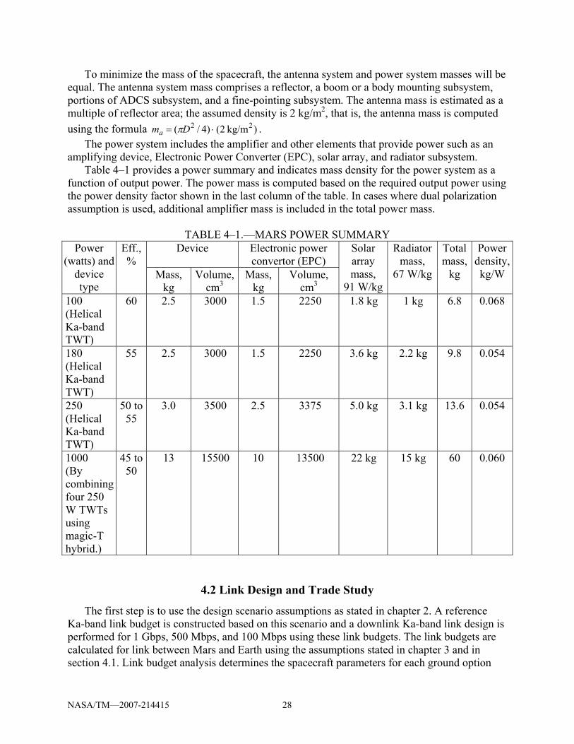
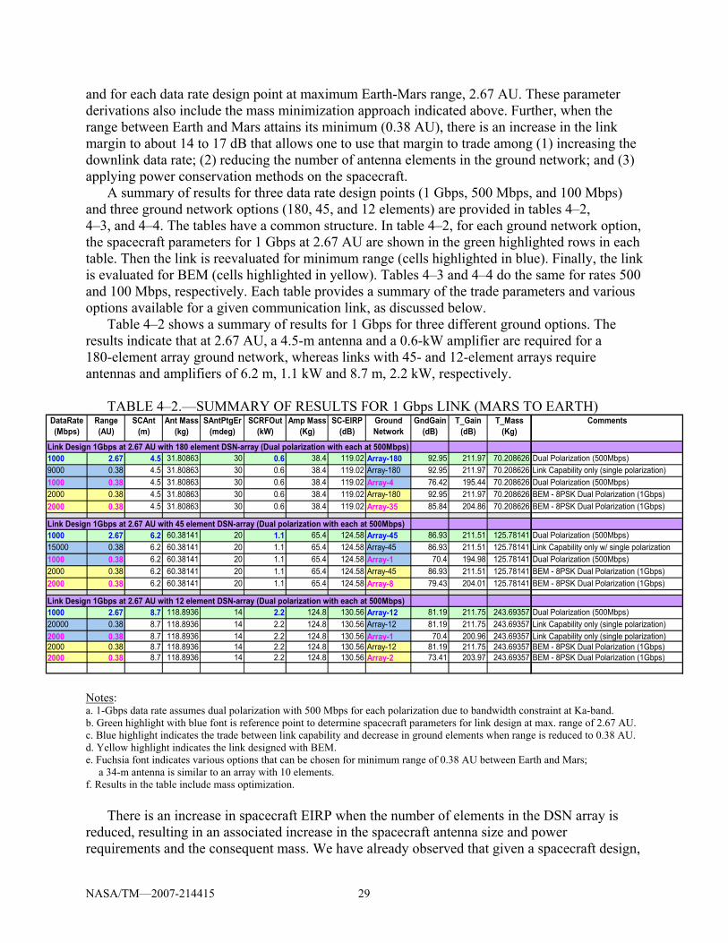
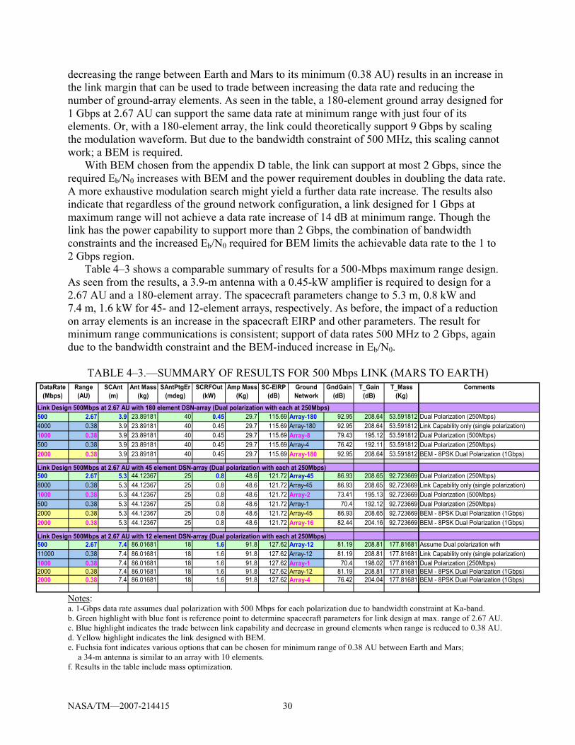
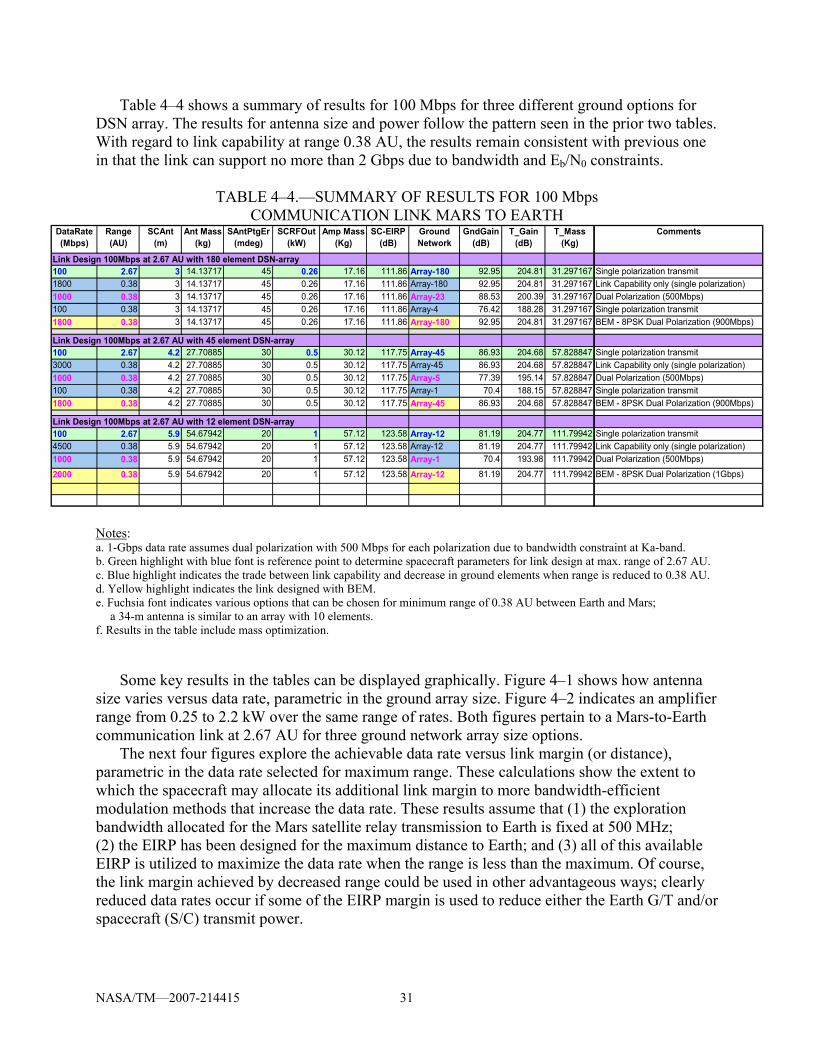
4.1 Design Approach ............................................................................................................... 27 4.2 Link Design and Trade Study............................................................................................ 28 4.3 Observations Concerning the Link Design Trade Study ................................................... 35 4.4 Conclusions Concerning the Link Design Trade Study .................................................... 36
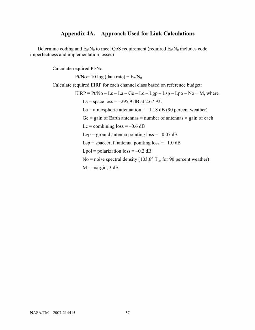
Appendix 4A.—Approach Used for Link Calculations................................................................ 37 Appendix 4B.—Some Options for Bandwidth-Efficient Modulation .......................................... 39 Appendix 4C.—Derivation of Mass Optimization, Given a Required EIRP ............................... 41
4C.1 Reference ........................................................................................................................ 42 5. Enabling Technologies for Earth-Mars Communications: Part I, Antenna System ................ 43
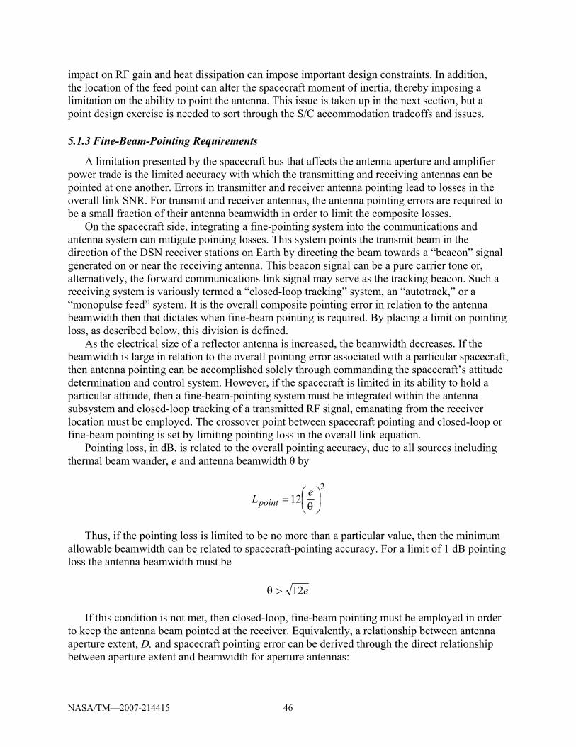
5.1 Antenna Requirements and the Antenna-ADCS Relationship .......................................... 44 5.1.1 Achieving 1 Gbps at Distance of 2.67 AU................................................................ 44 5.1.2 Spacecraft Accommodation ...................................................................................... 45 5.1.3 Fine-Beam-Pointing Requirements........................................................................... 46 5.1.4 ADCS Sizing............................................................................................................. 49
5.2 Large-Aperture Antenna Technologies and Architectures ................................................ 52 5.2.1 Overview of Current Antenna State of the Art and Future Research Directions...... 52
5.2.1.2 Reflectarrays ..................................................................................................................... 54 5.2.1.3 Active Phased-Array Antennas......................................................................................... 55 5.2.1.4 Discrete Element Lens Antennas ...................................................................................... 56
5.2.2 Reflector Antenna Designs to Enable Fine-Beam Pointing...................................... 56 5.2.2.1 Feed System Concepts to Enable Fine-Beam Steering.................................. 57 5.2.2.2 Synergy With Current State of the Art Antenna Developments.................... 61
5.5 References ......................................................................................................................... 93 6. Enabling Technologies for Earth-Mars Communications: Part II, Power
System Technologies................................................................................................................ 97 6.1 Power Requirements.......................................................................................................... 97 6.2 RF Amplifier and Power Combining................................................................................. 98
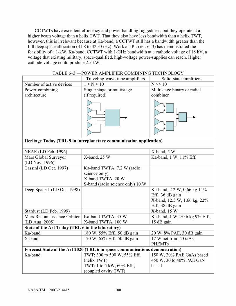
6.2.1 Traveling-Wave-Tube-Amplifiers ............................................................................ 99 6.2.1.1 Very High Power Amplifiers......................................................................... 99 6.2.1.2 Power-Combining Techniques .................................................................... 102
6.2.3 Summary of RF Amplifier and Power-Combining Technology and Solid-State Power Amplifier (SSPA) Technology..................................................................... 112
6.3 Solar Panels and Power Modules .................................................................................... 114 6.3.1 Solar Panels............................................................................................................. 114
6.3.2 Power Modules ....................................................................................................... 115 6.3.2.1 Battery Technology ..................................................................................... 116 6.3.2.2 Regenerative Fuel Cells............................................................................... 117 6.3.2.3 Flywheel Energy Storage System................................................................ 117 6.3.2.4 Power System Technology Assessment ...................................................... 118
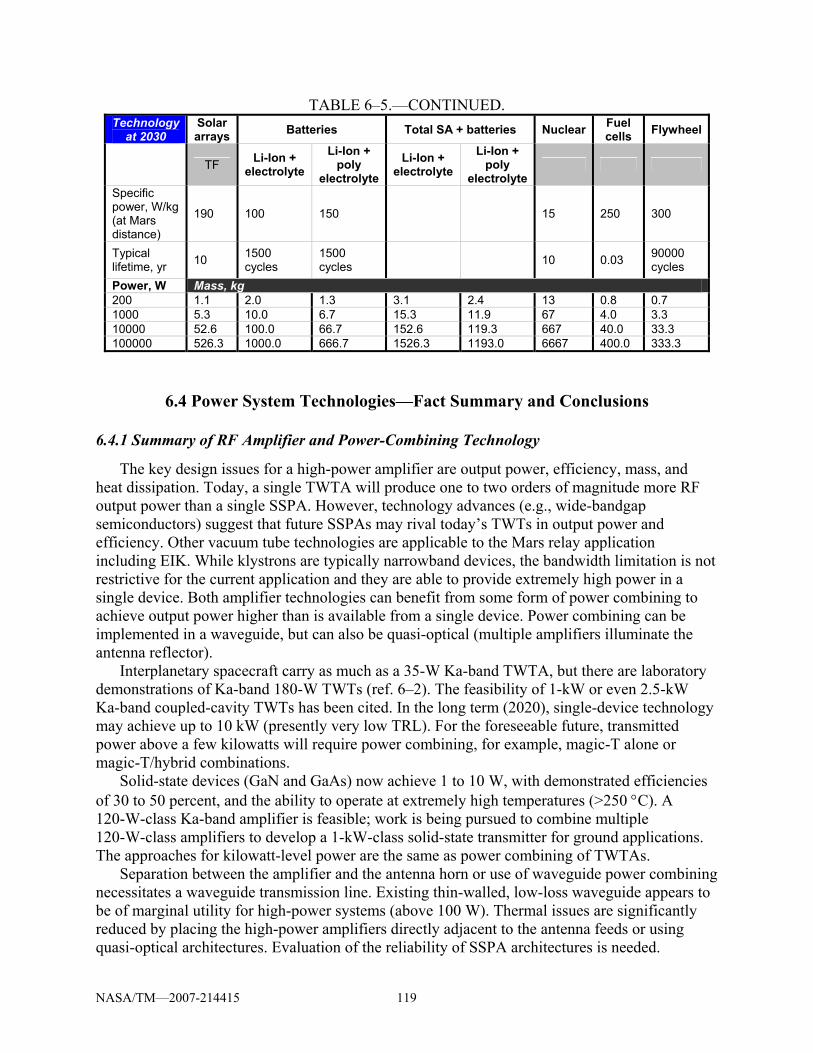
6.4 Power System Technologies—Fact Summary and Conclusions..................................... 119 6.4.1 Summary of RF Amplifier and Power-Combining Technology............................. 119 6.4.2. Summary of Solar Panel and Power-Module Technology..................................... 120
6.4.2.1 Solar Panels ................................................................................................. 120 6.4.2.2 Power Modules ............................................................................................ 120
6.5 Complexity of the Power Subsystem............................................................................... 120 6.6 References ....................................................................................................................... 120
7. Technology Complexity and Mass Minimization Approaches .............................................. 123 7.1 Design Approach for Maximum Range........................................................................... 123
7.1.1 Technology Risk ..................................................................................................... 123 7.1.2 The Global Minimum Mass Design Solution ......................................................... 125 7.1.3 Near-Optimum Total Mass Solutions ..................................................................... 126
7.2 Optimum Mass Subject to Minimization of Technology Complexity ............................ 126 7.2.1 The Mass-Technology Trade Space and Technical Approach ............................... 126
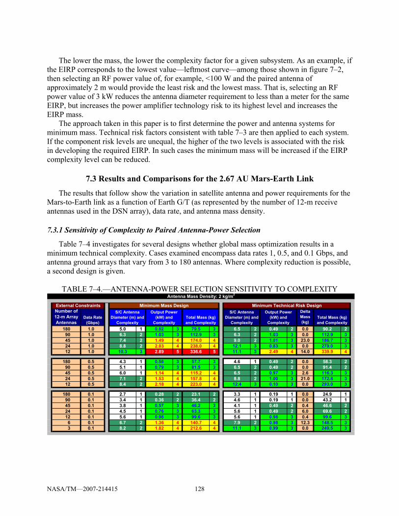
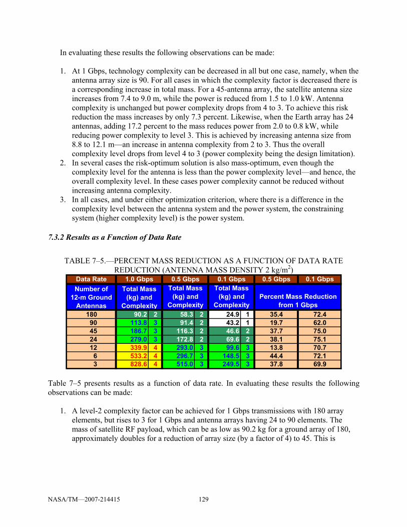
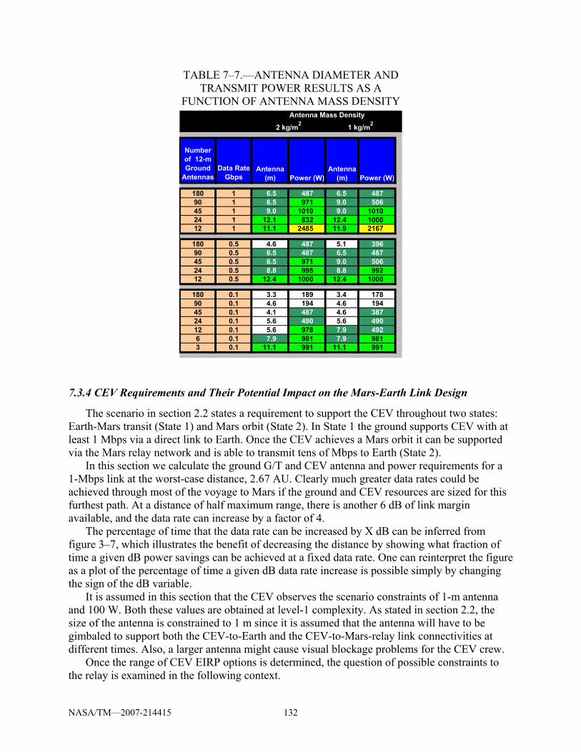
7.3 Results and Comparisons for the 2.67 AU Mars-Earth Link .......................................... 128 7.3.1 Sensitivity of Complexity to Paired Antenna-Power Selection .............................. 128 7.3.2 Results as a Function of Data Rate ......................................................................... 129 7.3.3 Results as a Function of Antenna Mass Density..................................................... 130 7.3.4 CEV Requirements and Their Potential Impact on the Mars-Earth Link Design... 132
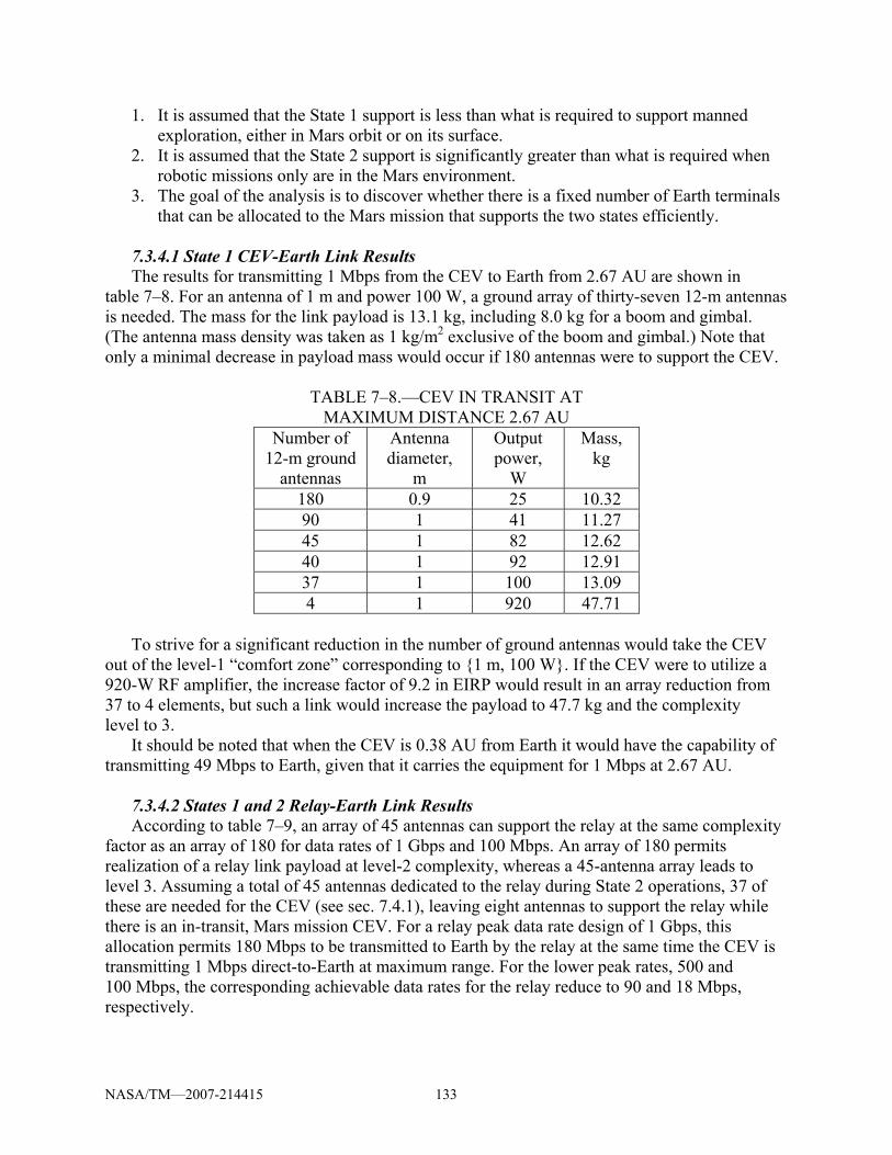
7.3.4.1 State 1 CEV-Earth Link Results .................................................................. 133 7.3.4.2 States 1 and 2 Relay-Earth Link Results ..................................................... 133
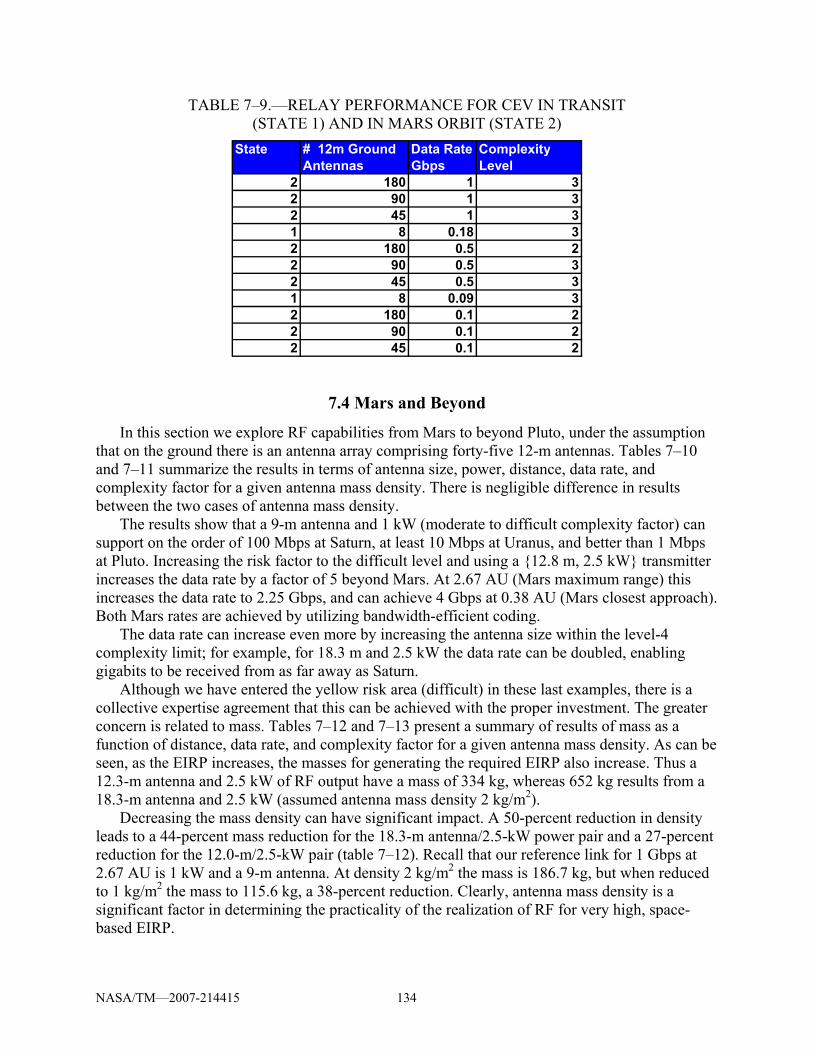
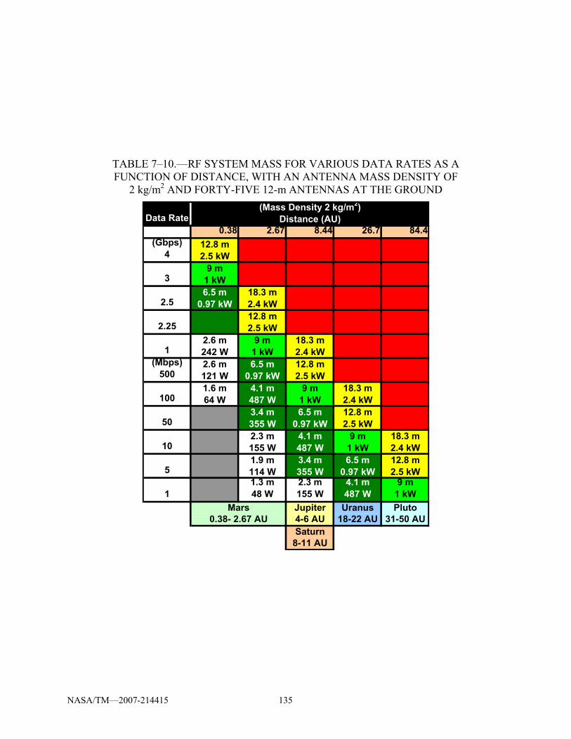
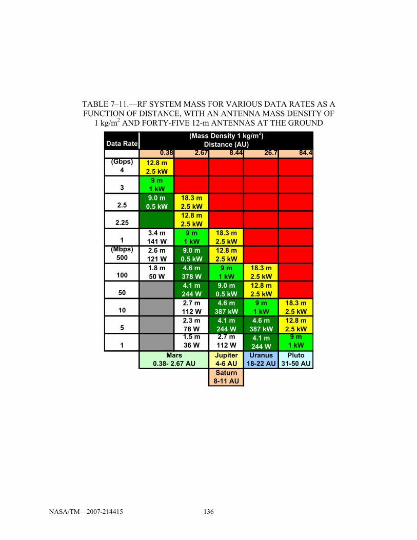
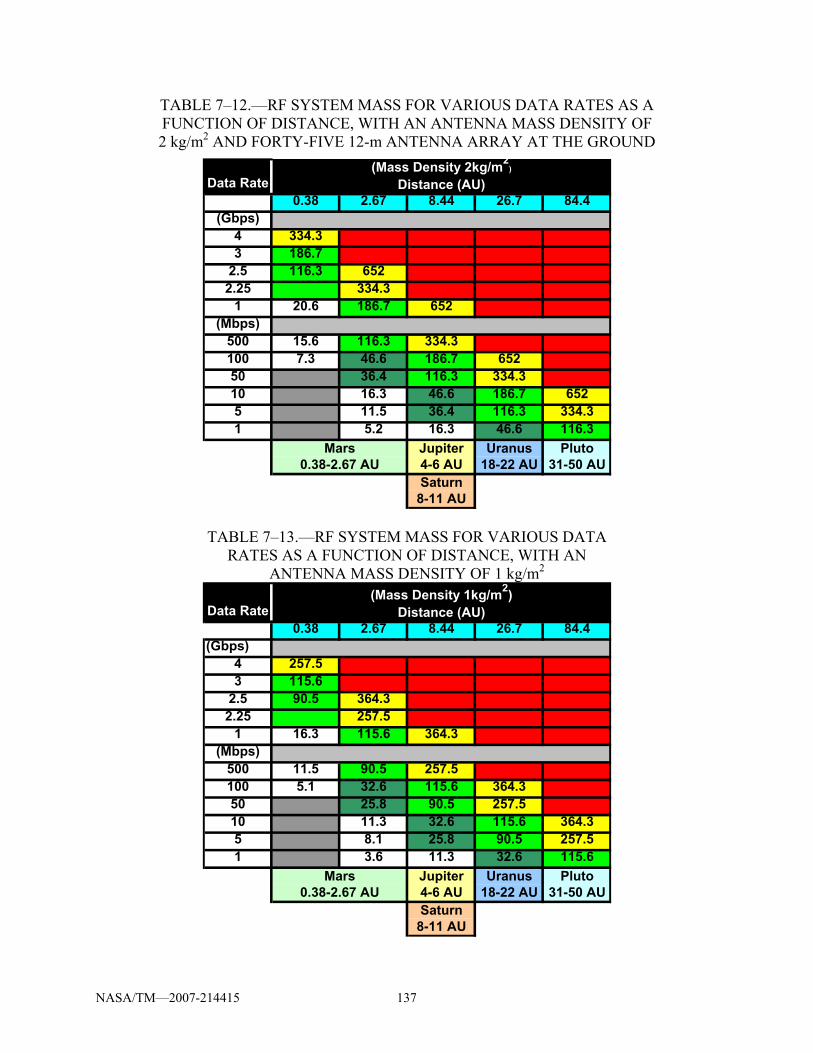
7.4 Mars and Beyond............................................................................................................. 134 7.4.1 Conclusions............................................................................................................. 138 7.4.2. Recommendations .................................................................................................. 138
7.5 Reference ......................................................................................................................... 138 Appendix 7A.—Antenna/Power System Mass Allocation Optimization for
Suboptimum Total Mass ........................................................................................................ 139 8. Conclusions and Recommendations ....................................................................................... 141
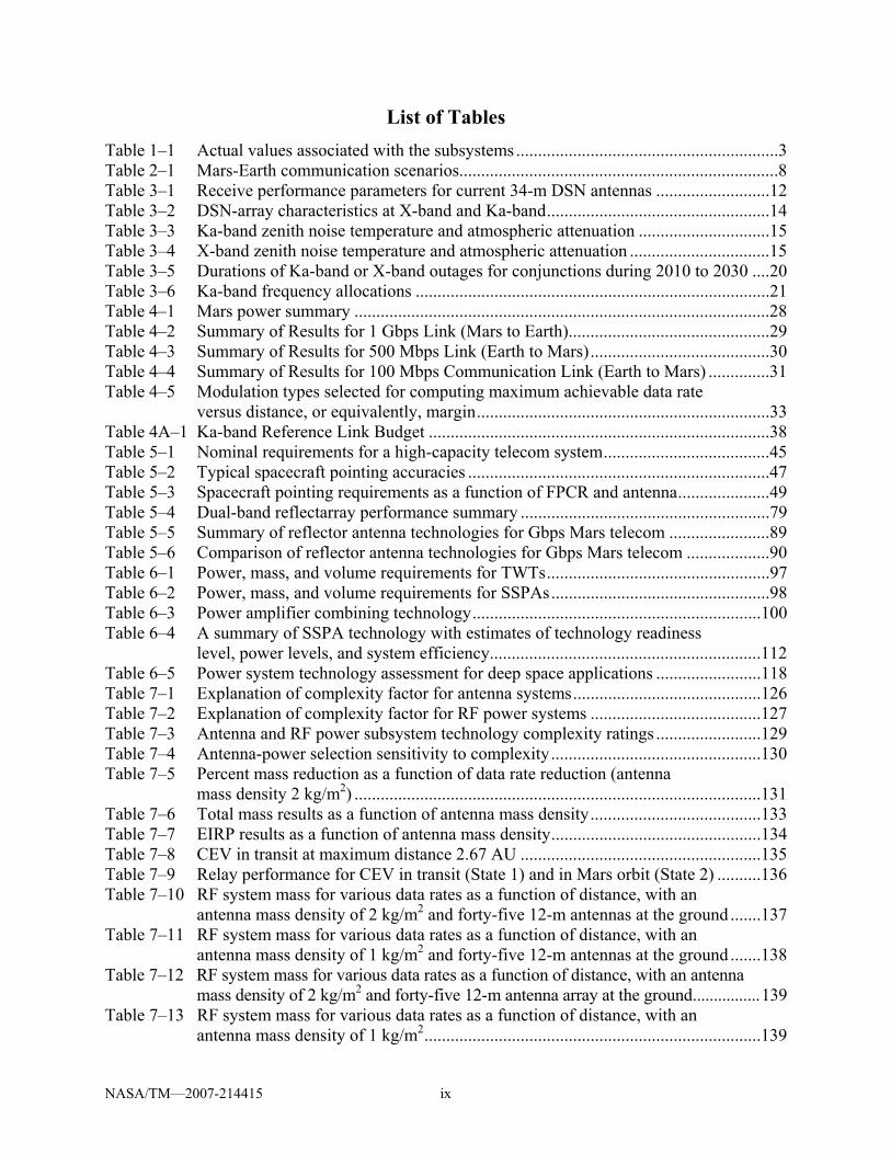
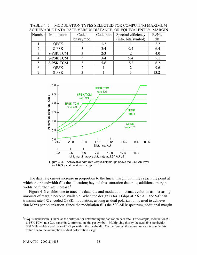
List of Tables Table 1–1 Actual values associated with the subsystems ............................................................3 Table 2–1 Mars-Earth communication scenarios.........................................................................8 Table 3–1 Receive performance parameters for current 34-m DSN antennas ..........................12 Table 3–2 DSN-array characteristics at X-band and Ka-band...................................................14 Table 3–3 Ka-band zenith noise temperature and atmospheric attenuation ..............................15 Table 3–4 X-band zenith noise temperature and atmospheric attenuation ................................15 Table 3–5 Durations of Ka-band or X-band outages for conjunctions during 2010 to 2030 ....20 Table 3–6 Ka-band frequency allocations .................................................................................21 Table 4–1 Mars power summary ...............................................................................................28 Table 4–2 Summary of Results for 1 Gbps Link (Mars to Earth)..............................................29 Table 4–3 Summary of Results for 500 Mbps Link (Earth to Mars).........................................30 Table 4–4 Summary of Results for 100 Mbps Communication Link (Earth to Mars) ..............31 Table 4–5 Modulation types selected for computing maximum achievable data rate
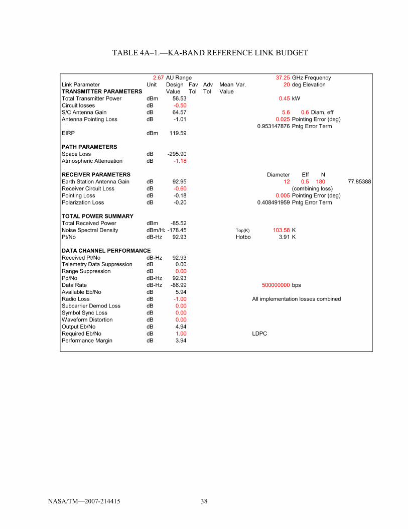
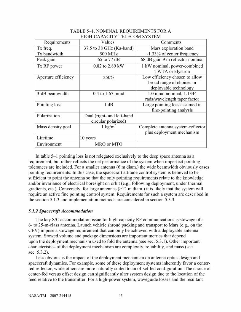
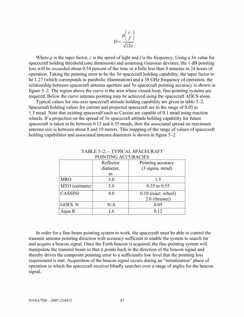
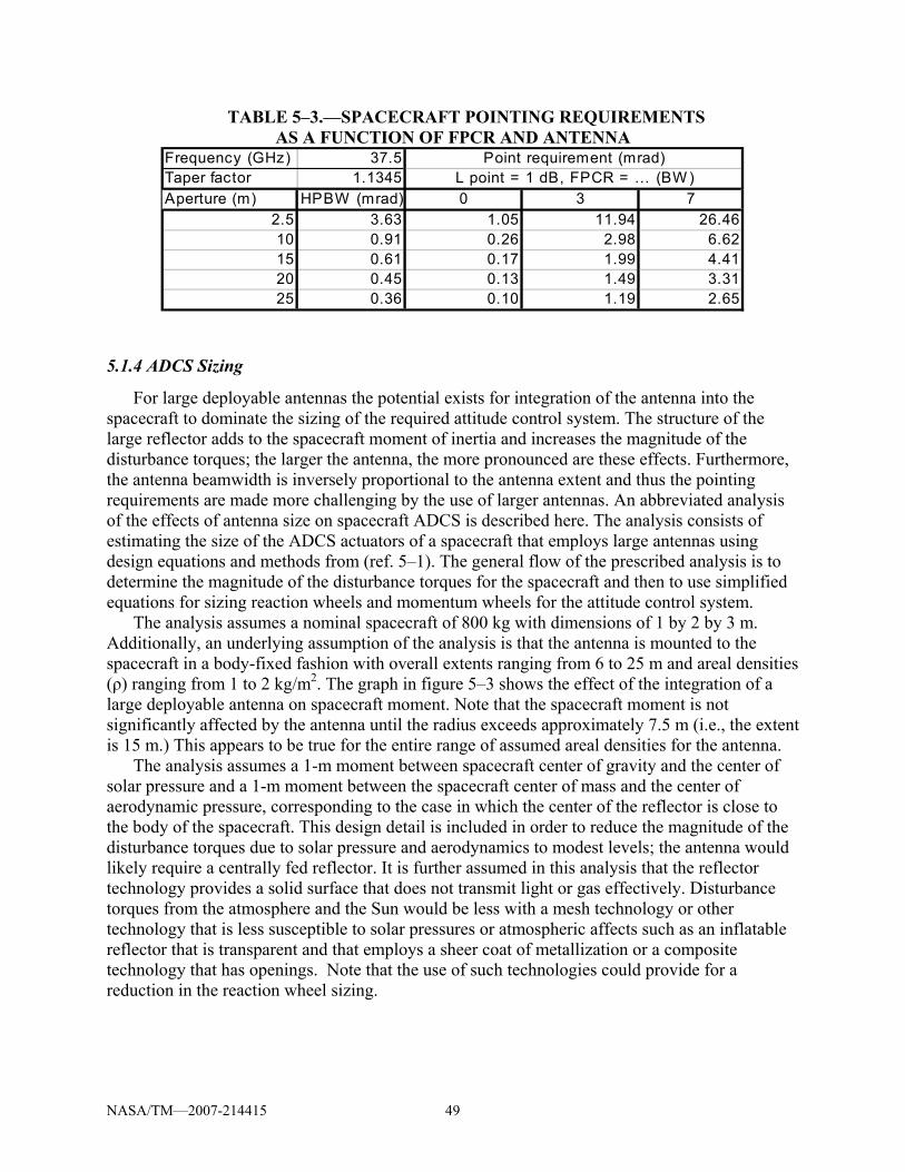
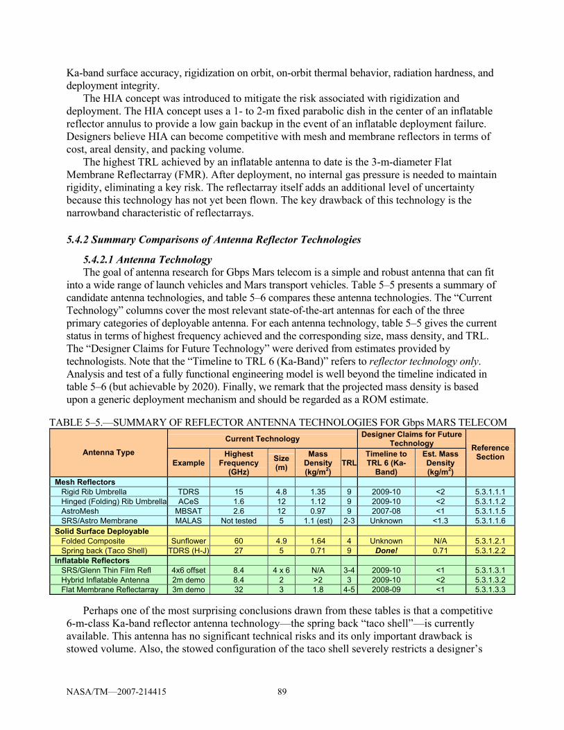
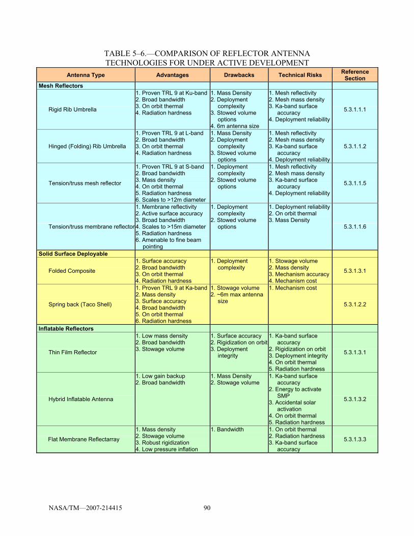
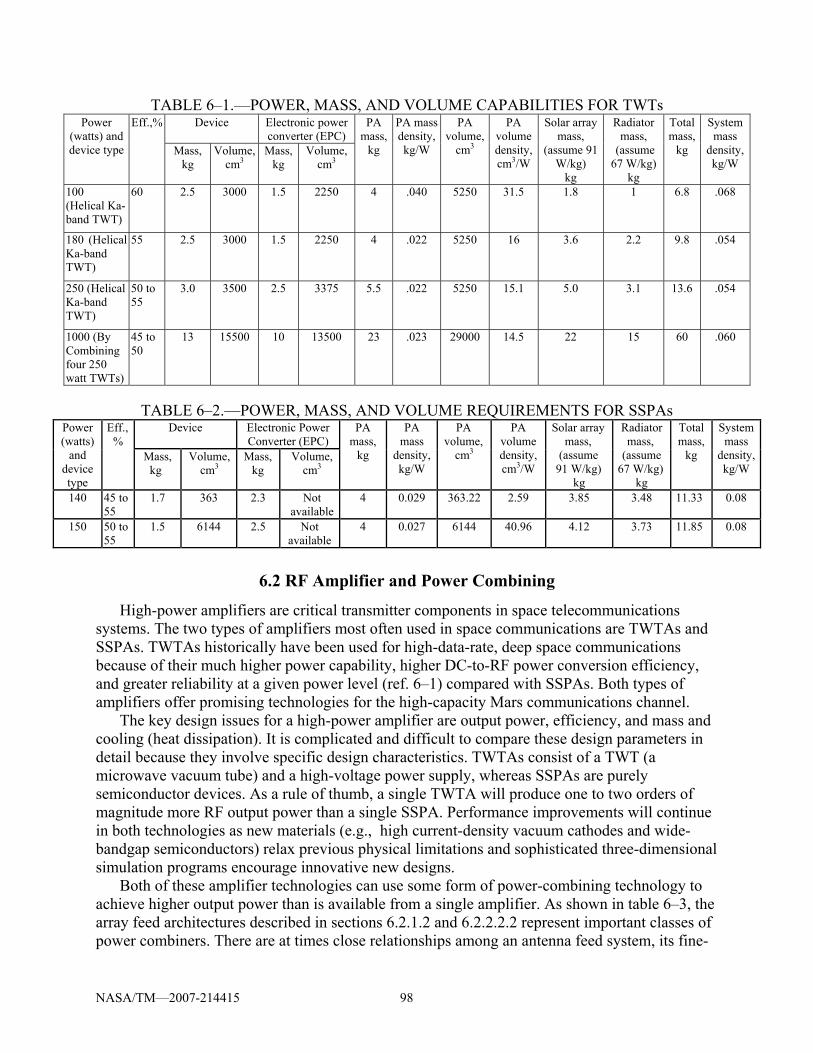
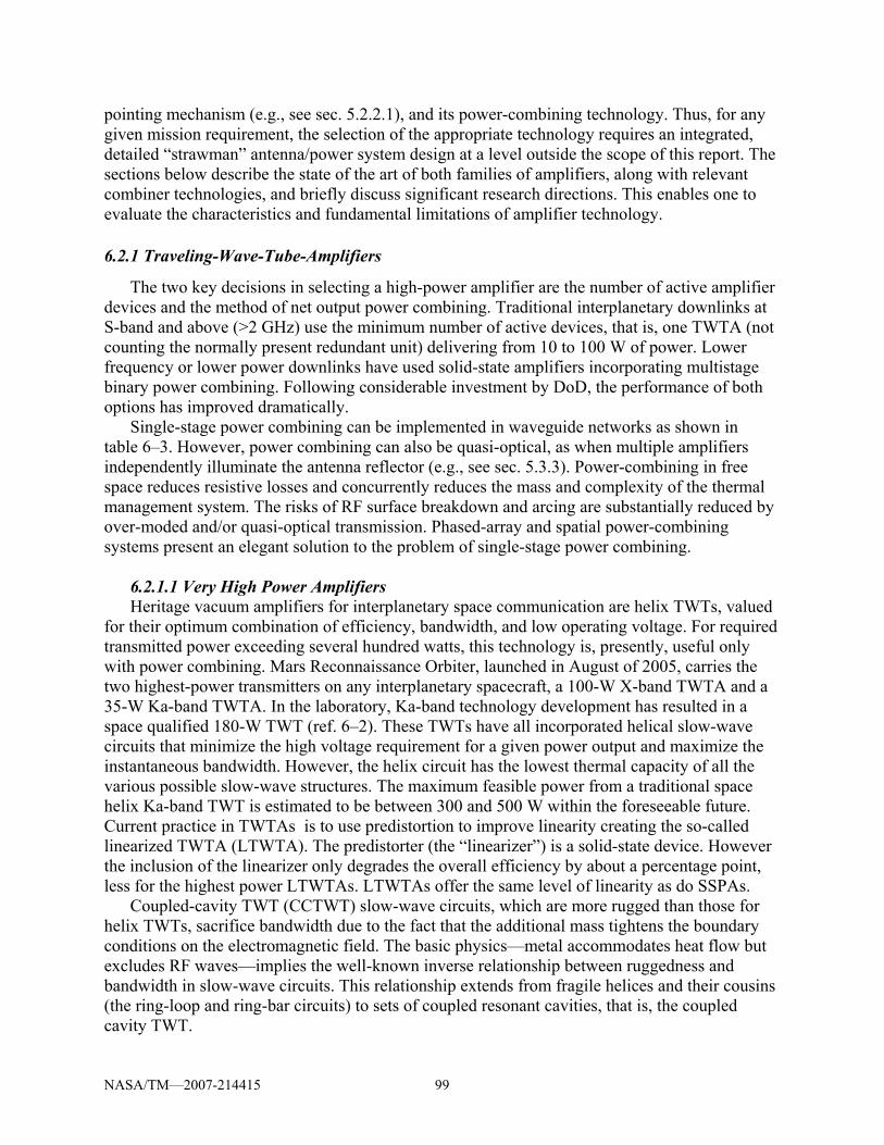
versus distance, or equivalently, margin...................................................................33 Table 4A–1 Ka-band Reference Link Budget ..............................................................................38 Table 5–1 Nominal requirements for a high-capacity telecom system......................................45 Table 5–2 Typical spacecraft pointing accuracies .....................................................................47 Table 5–3 Spacecraft pointing requirements as a function of FPCR and antenna.....................49 Table 5–4 Dual-band reflectarray performance summary .........................................................79 Table 5–5 Summary of reflector antenna technologies for Gbps Mars telecom .......................89 Table 5–6 Comparison of reflector antenna technologies for Gbps Mars telecom ...................90 Table 6–1 Power, mass, and volume requirements for TWTs...................................................97 Table 6–2 Power, mass, and volume requirements for SSPAs..................................................98 Table 6–3 Power amplifier combining technology..................................................................100 Table 6–4 A summary of SSPA technology with estimates of technology readiness
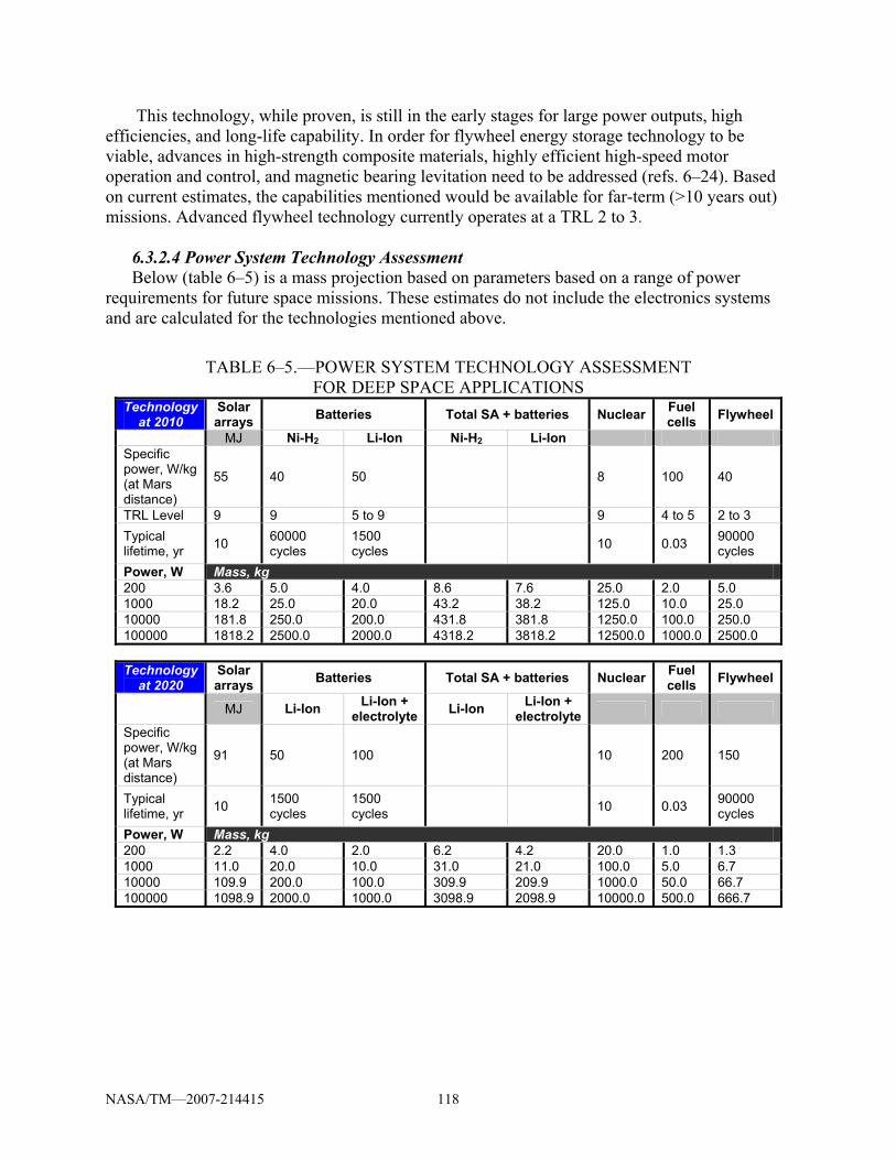
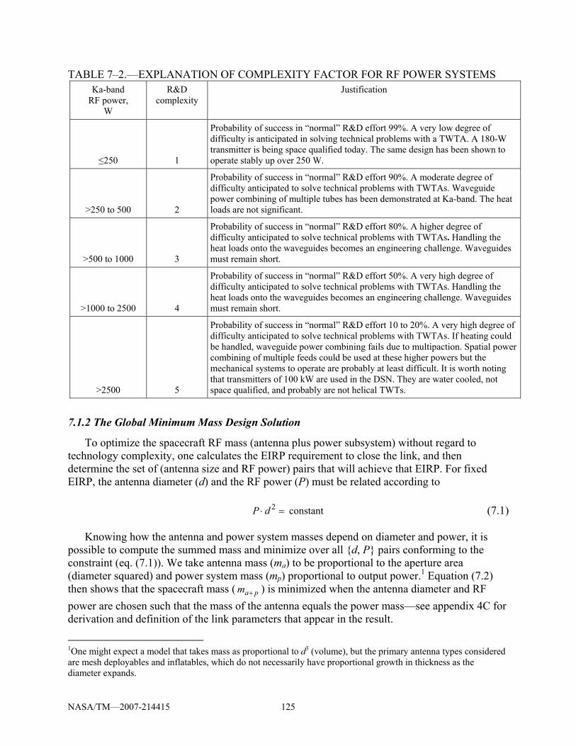
level, power levels, and system efficiency..............................................................112 Table 6–5 Power system technology assessment for deep space applications ........................118 Table 7–1 Explanation of complexity factor for antenna systems...........................................126 Table 7–2 Explanation of complexity factor for RF power systems .......................................127 Table 7–3 Antenna and RF power subsystem technology complexity ratings ........................129 Table 7–4 Antenna-power selection sensitivity to complexity................................................130 Table 7–5 Percent mass reduction as a function of data rate reduction (antenna
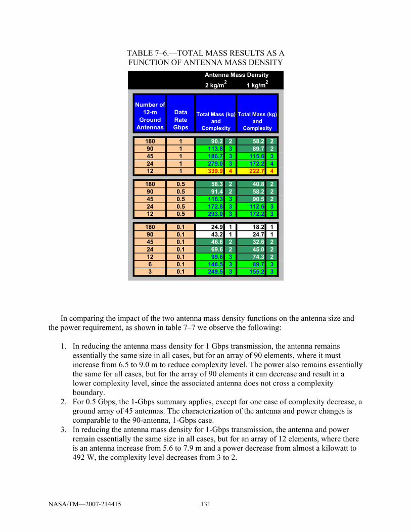
mass density 2 kg/m2) .............................................................................................131 Table 7–6 Total mass results as a function of antenna mass density.......................................133 Table 7–7 EIRP results as a function of antenna mass density................................................134 Table 7–8 CEV in transit at maximum distance 2.67 AU .......................................................135 Table 7–9 Relay performance for CEV in transit (State 1) and in Mars orbit (State 2) ..........136 Table 7–10 RF system mass for various data rates as a function of distance, with an
antenna mass density of 2 kg/m2 and forty-five 12-m antennas at the ground .......137 Table 7–11 RF system mass for various data rates as a function of distance, with an
antenna mass density of 1 kg/m2 and forty-five 12-m antennas at the ground .......138 Table 7–12 RF system mass for various data rates as a function of distance, with an antenna
mass density of 2 kg/m2 and forty-five 12-m antenna array at the ground................139 Table 7–13 RF system mass for various data rates as a function of distance, with an
antenna mass density of 1 kg/m2.............................................................................139
NASA/TM—2007-214415 xi
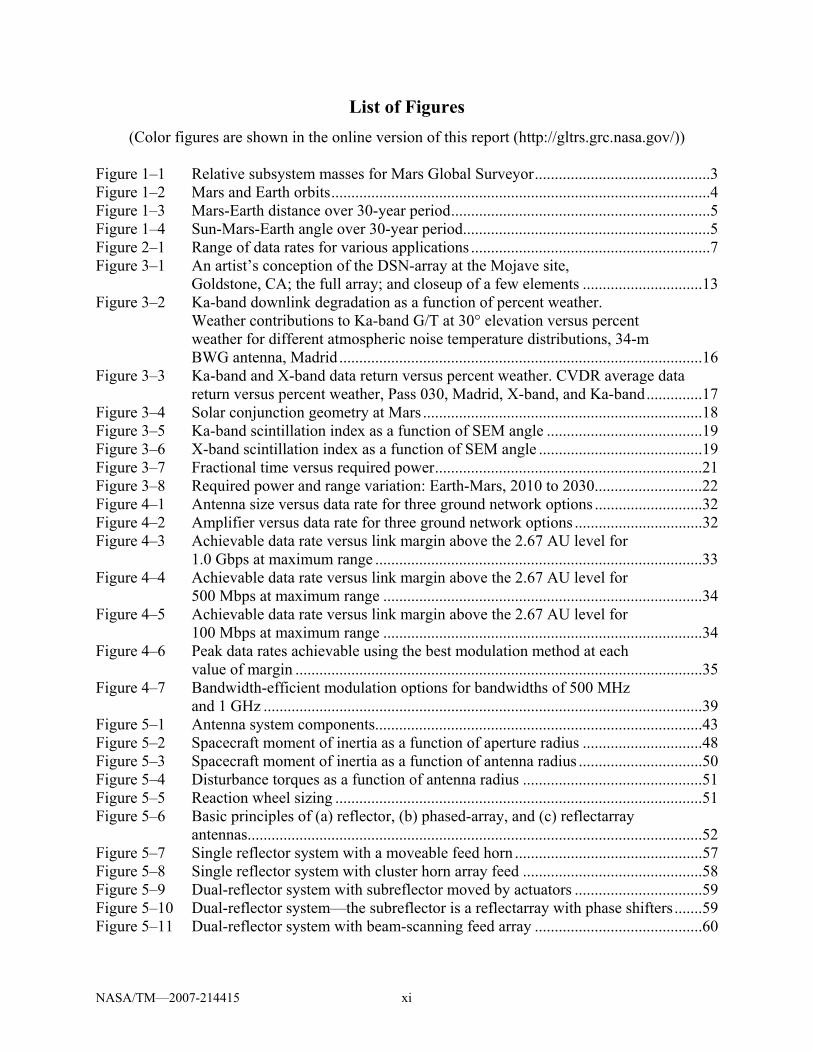
List of Figures (Color figures are shown in the online version of this report (http://gltrs.grc.nasa.gov/))
Figure 1–1 Relative subsystem masses for Mars Global Surveyor............................................3 Figure 1–2 Mars and Earth orbits...............................................................................................4 Figure 1–3 Mars-Earth distance over 30-year period.................................................................5 Figure 1–4 Sun-Mars-Earth angle over 30-year period..............................................................5 Figure 2–1 Range of data rates for various applications ............................................................7 Figure 3–1 An artist’s conception of the DSN-array at the Mojave site,
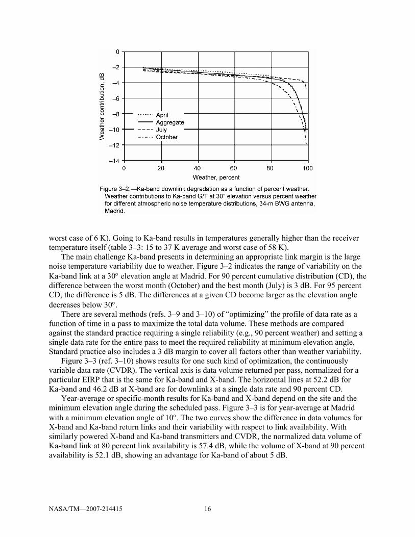
Goldstone, CA; the full array; and closeup of a few elements ..............................13 Figure 3–2 Ka-band downlink degradation as a function of percent weather.
Weather contributions to Ka-band G/T at 30° elevation versus percent weather for different atmospheric noise temperature distributions, 34-m BWG antenna, Madrid ...........................................................................................16
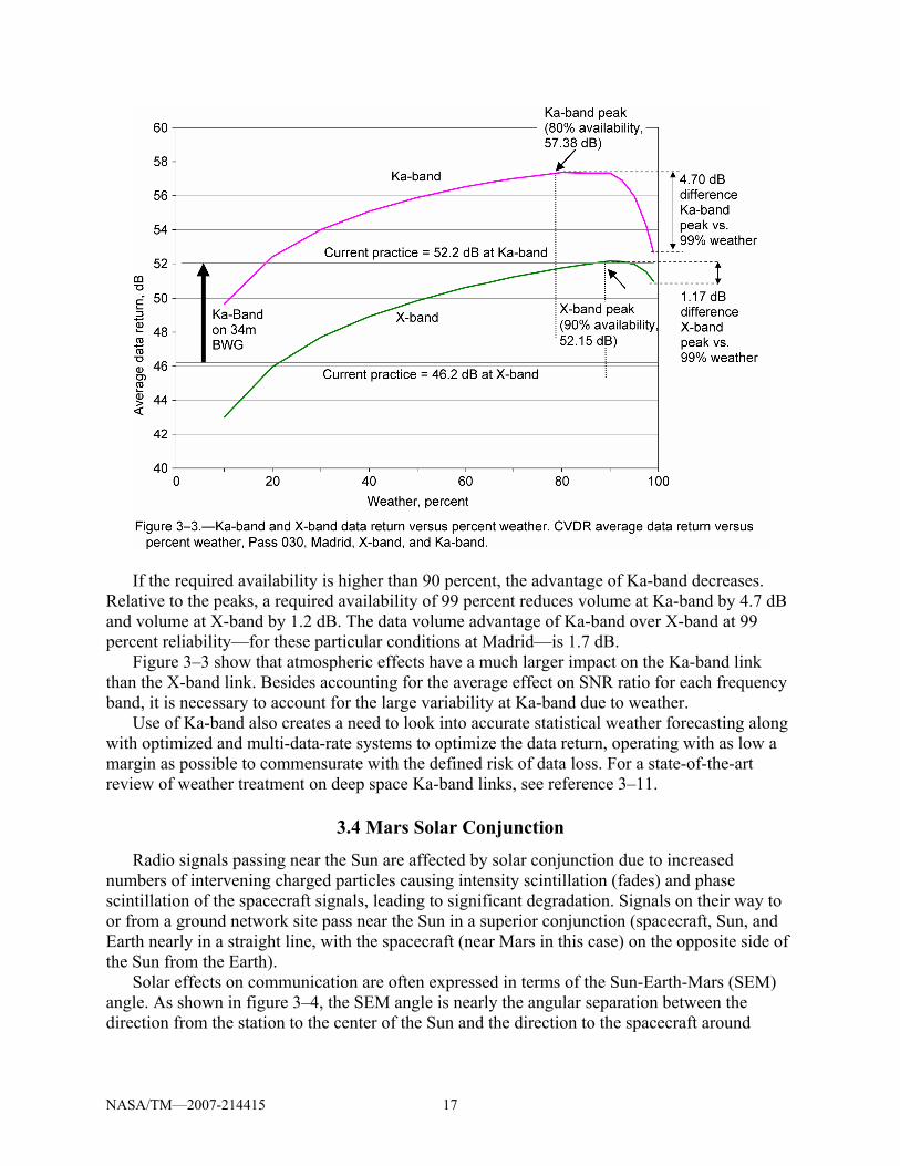
Figure 3–3 Ka-band and X-band data return versus percent weather. CVDR average data return versus percent weather, Pass 030, Madrid, X-band, and Ka-band..............17
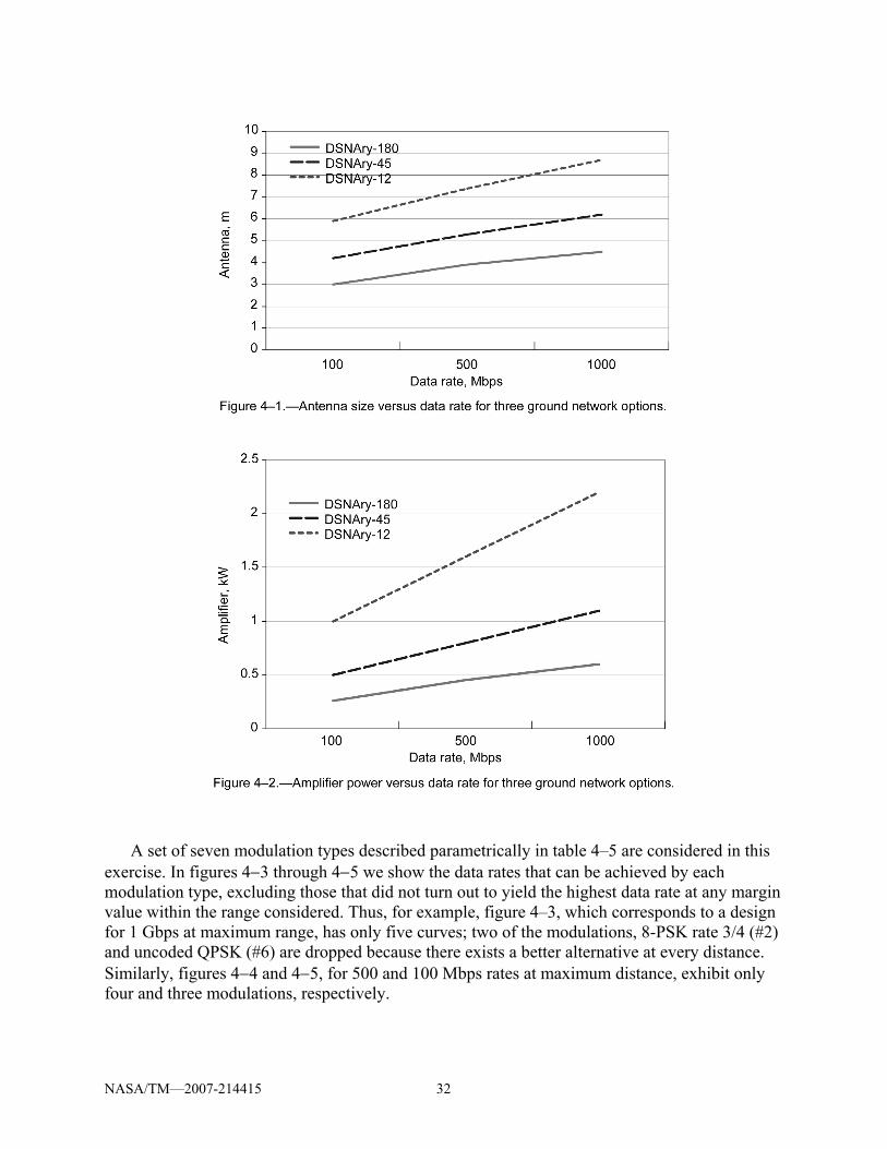
Figure 3–4 Solar conjunction geometry at Mars ......................................................................18 Figure 3–5 Ka-band scintillation index as a function of SEM angle .......................................19 Figure 3–6 X-band scintillation index as a function of SEM angle .........................................19 Figure 3–7 Fractional time versus required power...................................................................21 Figure 3–8 Required power and range variation: Earth-Mars, 2010 to 2030...........................22 Figure 4–1 Antenna size versus data rate for three ground network options ...........................32 Figure 4–2 Amplifier versus data rate for three ground network options ................................32 Figure 4–3 Achievable data rate versus link margin above the 2.67 AU level for
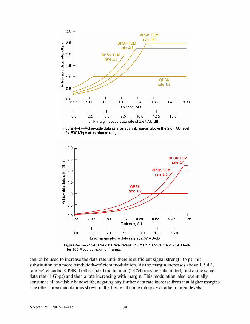
1.0 Gbps at maximum range ..................................................................................33 Figure 4–4 Achievable data rate versus link margin above the 2.67 AU level for
500 Mbps at maximum range ................................................................................34 Figure 4–5 Achievable data rate versus link margin above the 2.67 AU level for
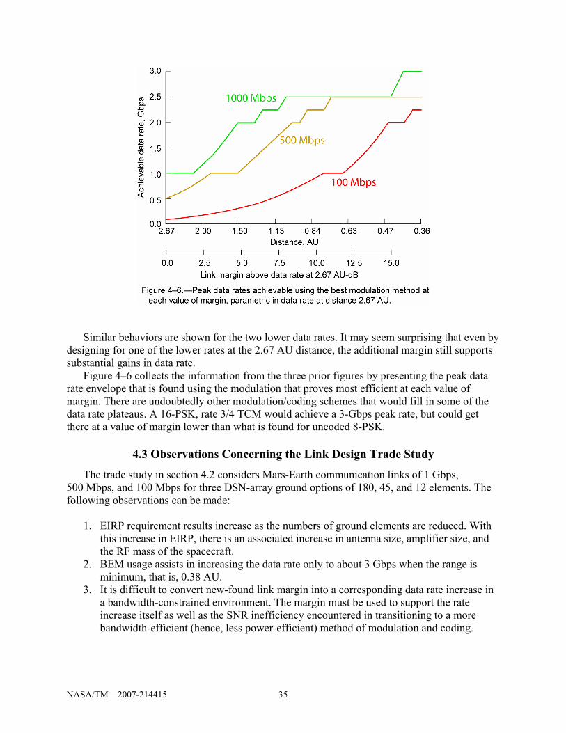
100 Mbps at maximum range ................................................................................34 Figure 4–6 Peak data rates achievable using the best modulation method at each
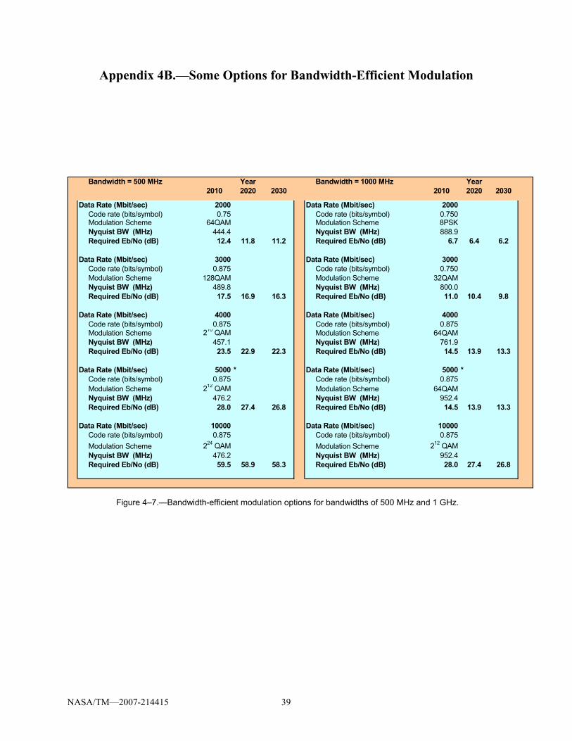
value of margin ......................................................................................................35 Figure 4–7 Bandwidth-efficient modulation options for bandwidths of 500 MHz
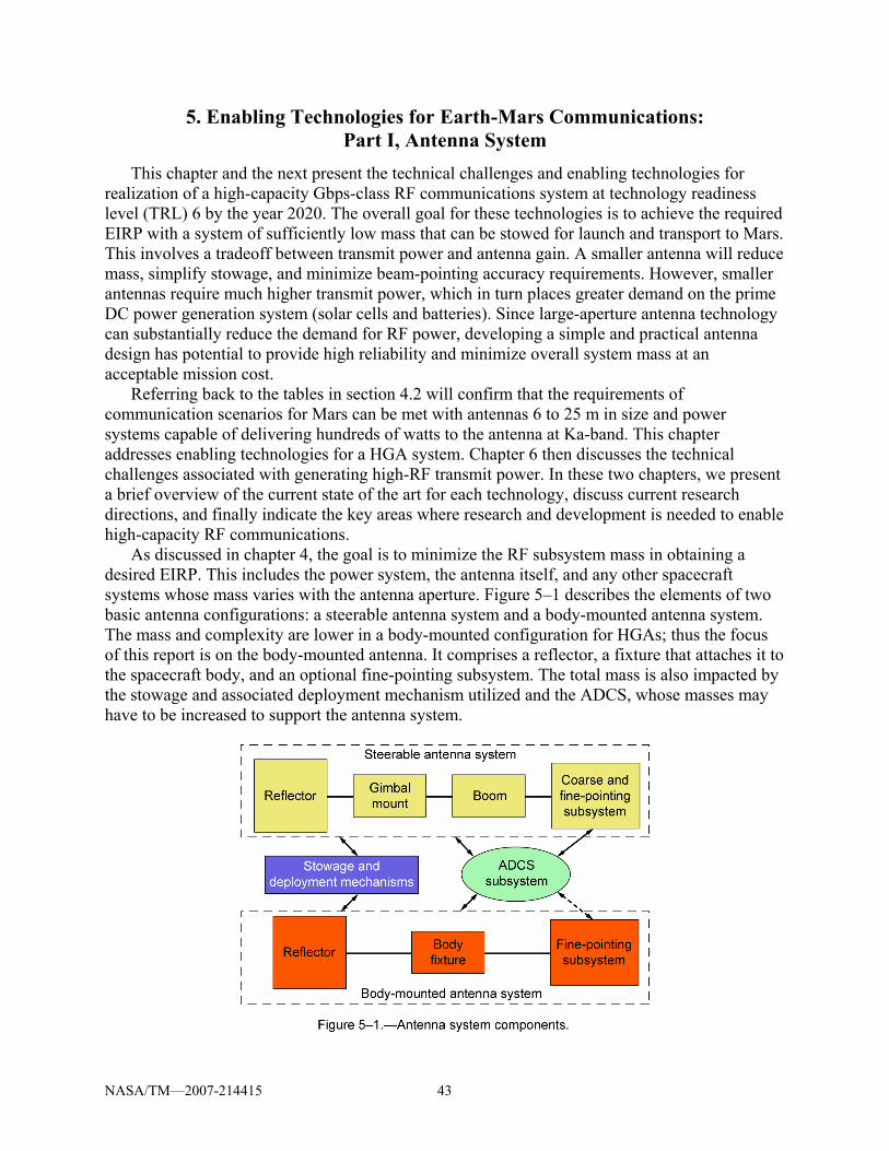
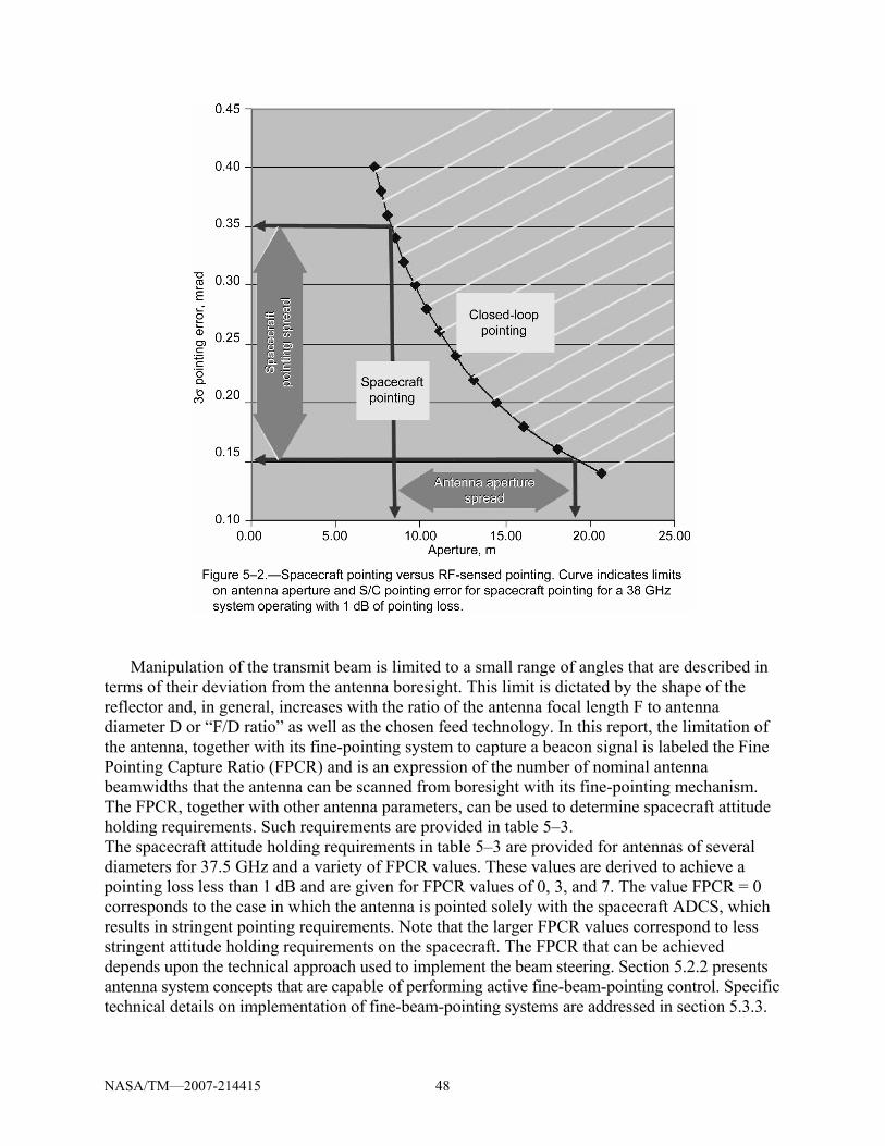
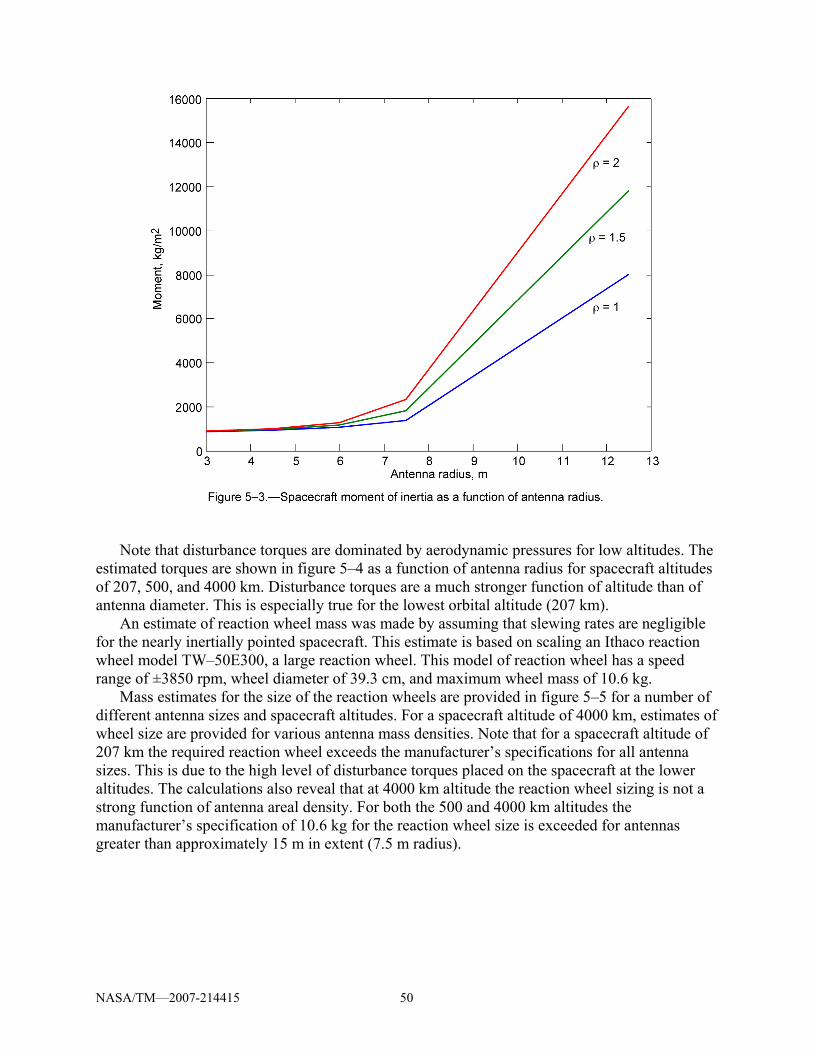
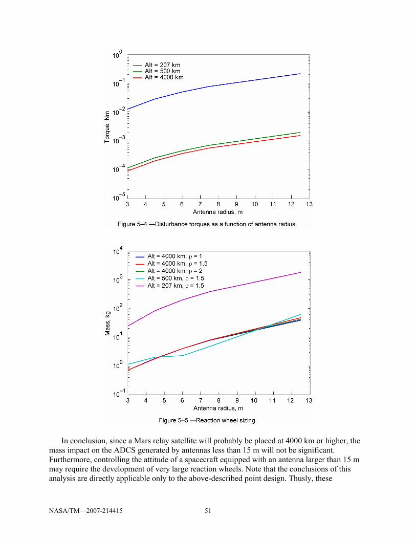
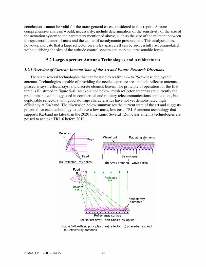
and 1 GHz ..............................................................................................................39 Figure 5–1 Antenna system components..................................................................................43 Figure 5–2 Spacecraft moment of inertia as a function of aperture radius ..............................48 Figure 5–3 Spacecraft moment of inertia as a function of antenna radius ...............................50 Figure 5–4 Disturbance torques as a function of antenna radius .............................................51 Figure 5–5 Reaction wheel sizing ............................................................................................51 Figure 5–6 Basic principles of (a) reflector, (b) phased-array, and (c) reflectarray
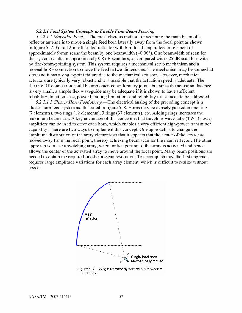
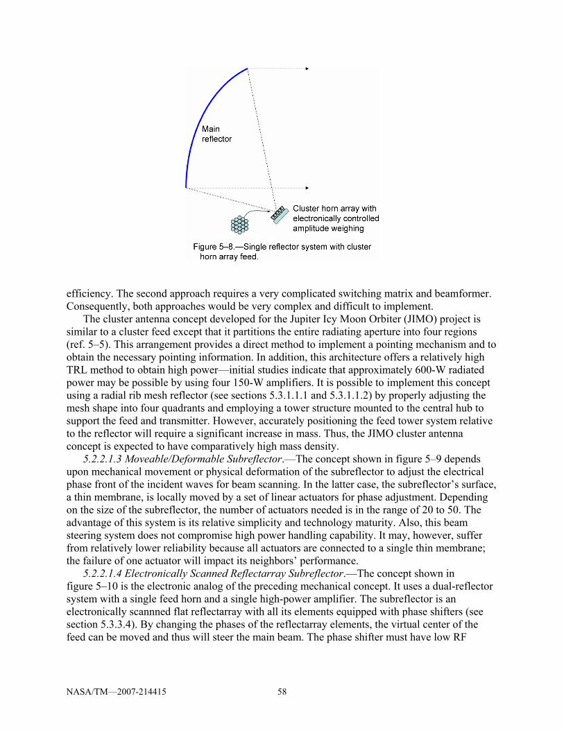
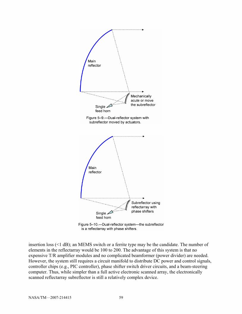
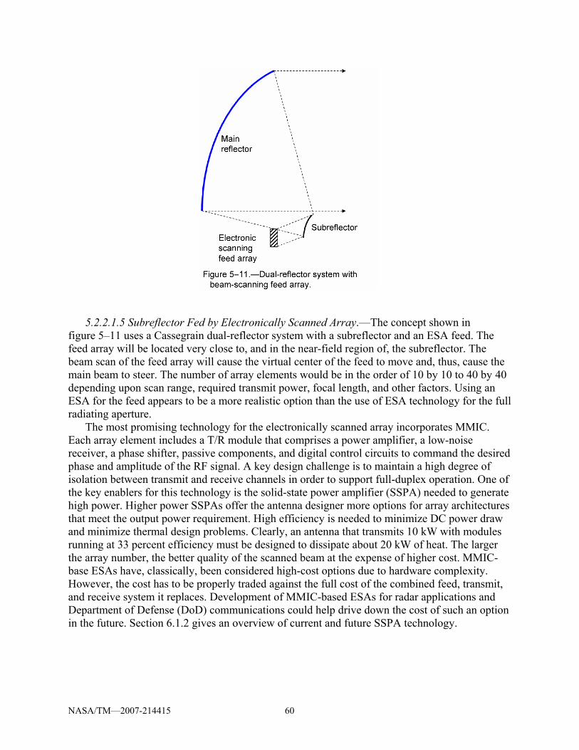
antennas..................................................................................................................52 Figure 5–7 Single reflector system with a moveable feed horn ...............................................57 Figure 5–8 Single reflector system with cluster horn array feed .............................................58 Figure 5–9 Dual-reflector system with subreflector moved by actuators ................................59 Figure 5–10 Dual-reflector system—the subreflector is a reflectarray with phase shifters .......59 Figure 5–11 Dual-reflector system with beam-scanning feed array ..........................................60
NASA/TM—2007-214415 xii
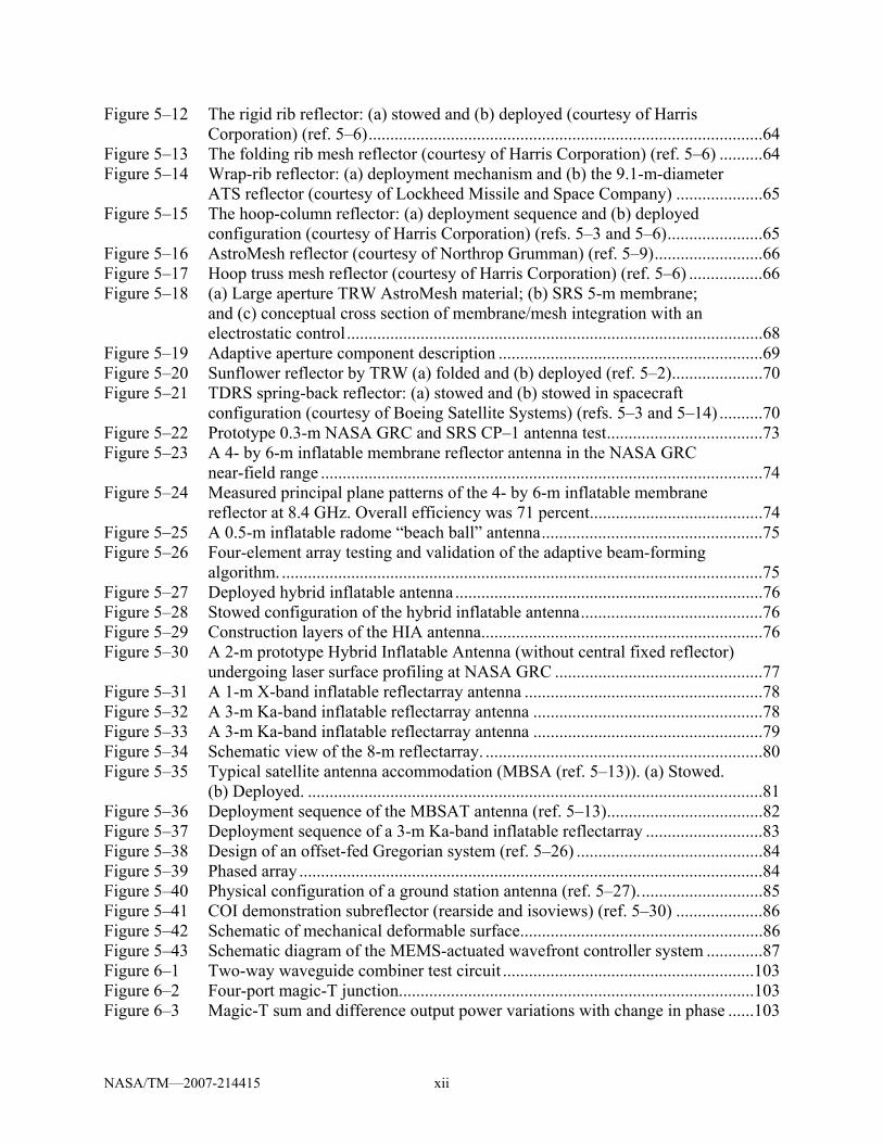
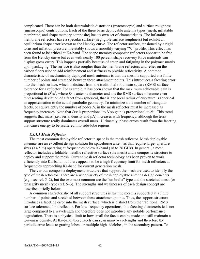
Figure 5–12 The rigid rib reflector: (a) stowed and (b) deployed (courtesy of Harris Corporation) (ref. 5–6)...........................................................................................64
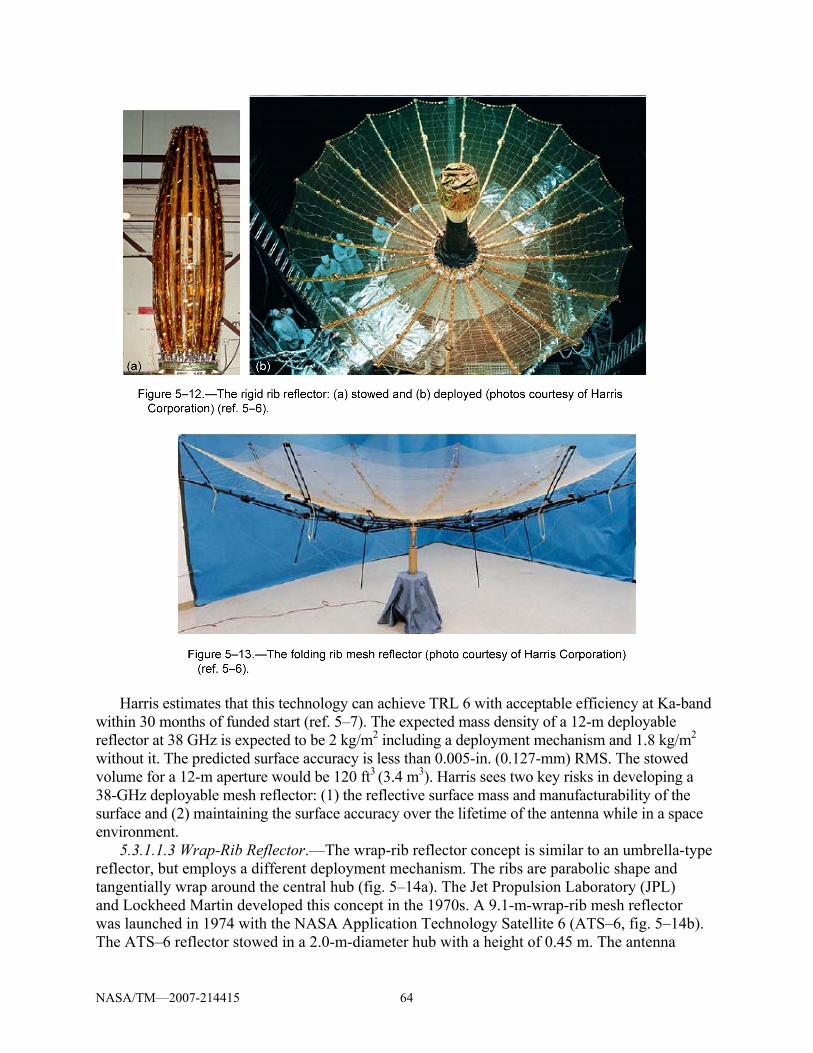
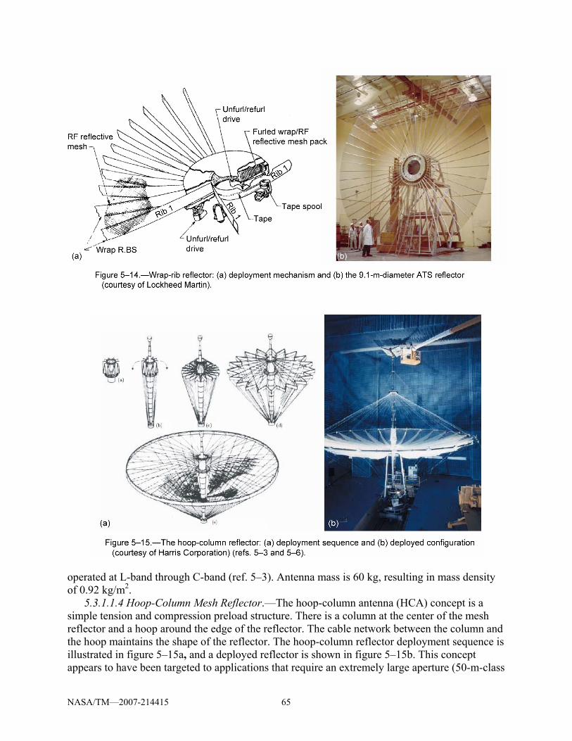
Figure 5–13 The folding rib mesh reflector (courtesy of Harris Corporation) (ref. 5–6) ..........64 Figure 5–14 Wrap-rib reflector: (a) deployment mechanism and (b) the 9.1-m-diameter
ATS reflector (courtesy of Lockheed Missile and Space Company) ....................65 Figure 5–15 The hoop-column reflector: (a) deployment sequence and (b) deployed
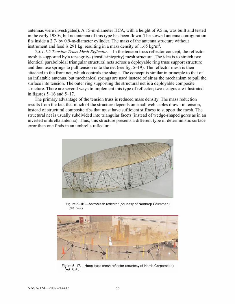
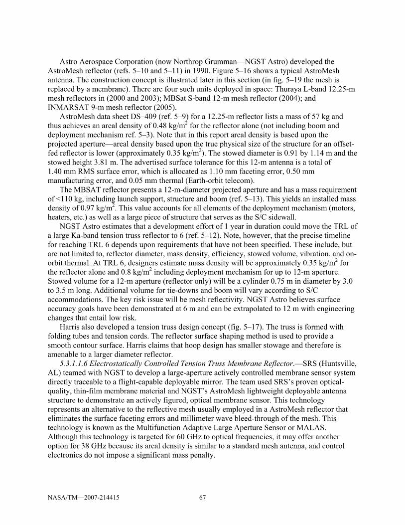
configuration (courtesy of Harris Corporation) (refs. 5–3 and 5–6)......................65 Figure 5–16 AstroMesh reflector (courtesy of Northrop Grumman) (ref. 5–9).........................66 Figure 5–17 Hoop truss mesh reflector (courtesy of Harris Corporation) (ref. 5–6) .................66 Figure 5–18 (a) Large aperture TRW AstroMesh material; (b) SRS 5-m membrane;
and (c) conceptual cross section of membrane/mesh integration with an electrostatic control................................................................................................68
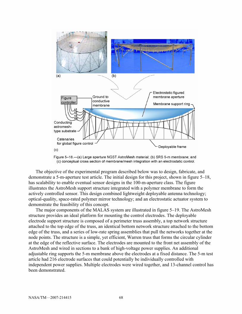
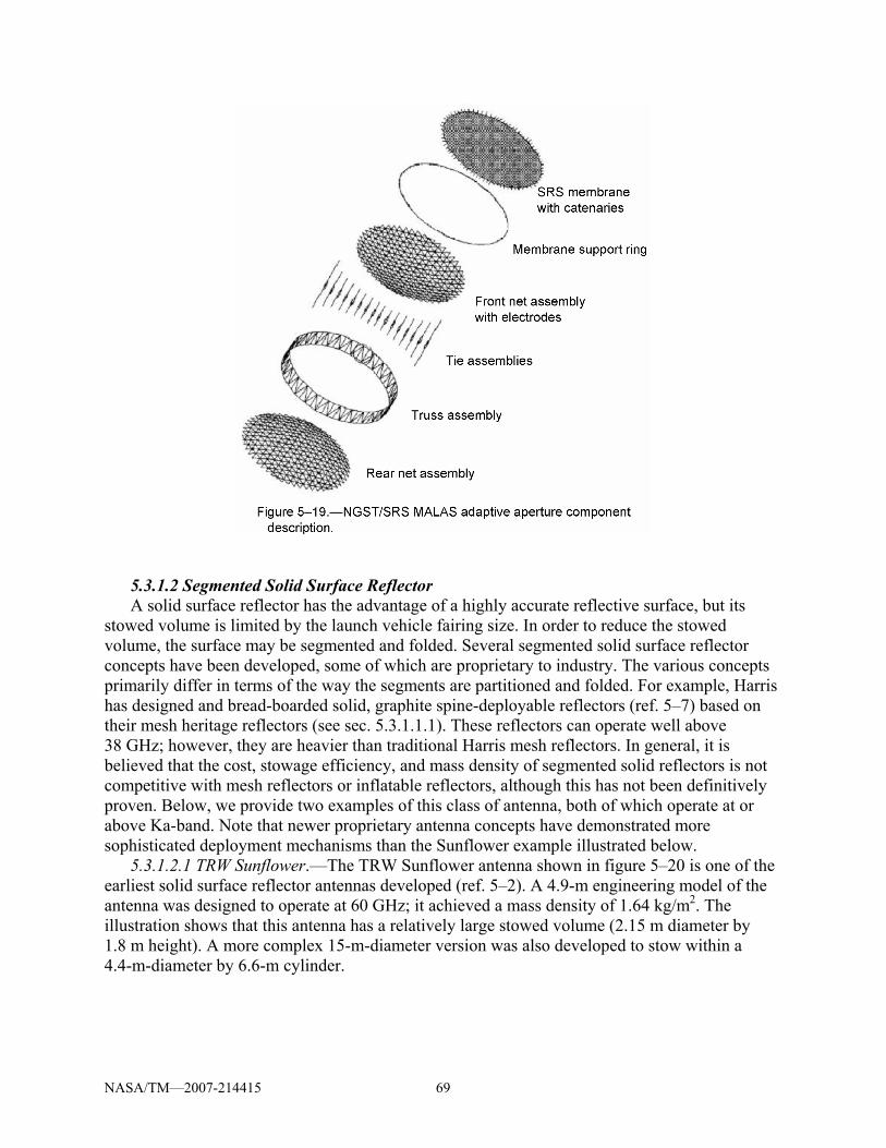
Figure 5–19 Adaptive aperture component description .............................................................69 Figure 5–20 Sunflower reflector by TRW (a) folded and (b) deployed (ref. 5–2).....................70 Figure 5–21 TDRS spring-back reflector: (a) stowed and (b) stowed in spacecraft
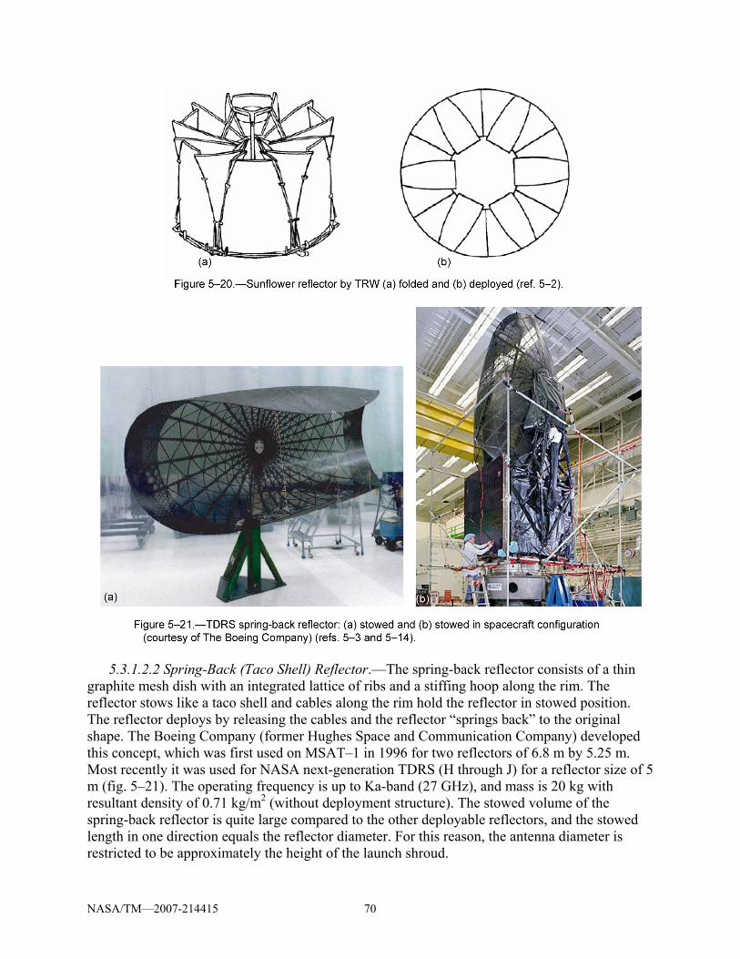
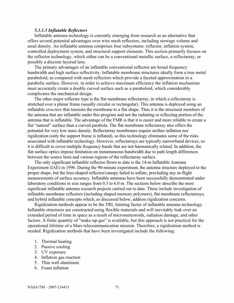
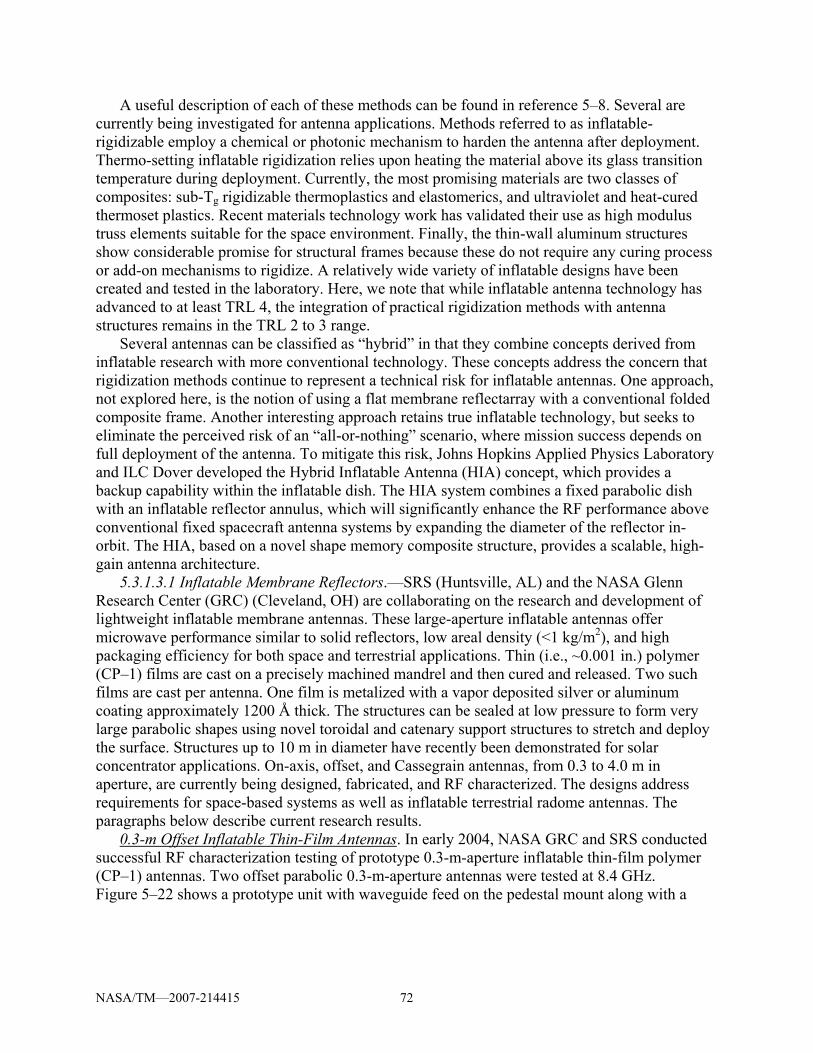
configuration (courtesy of Boeing Satellite Systems) (refs. 5–3 and 5–14) ..........70 Figure 5–22 Prototype 0.3-m NASA GRC and SRS CP–1 antenna test....................................73 Figure 5–23 A 4- by 6-m inflatable membrane reflector antenna in the NASA GRC
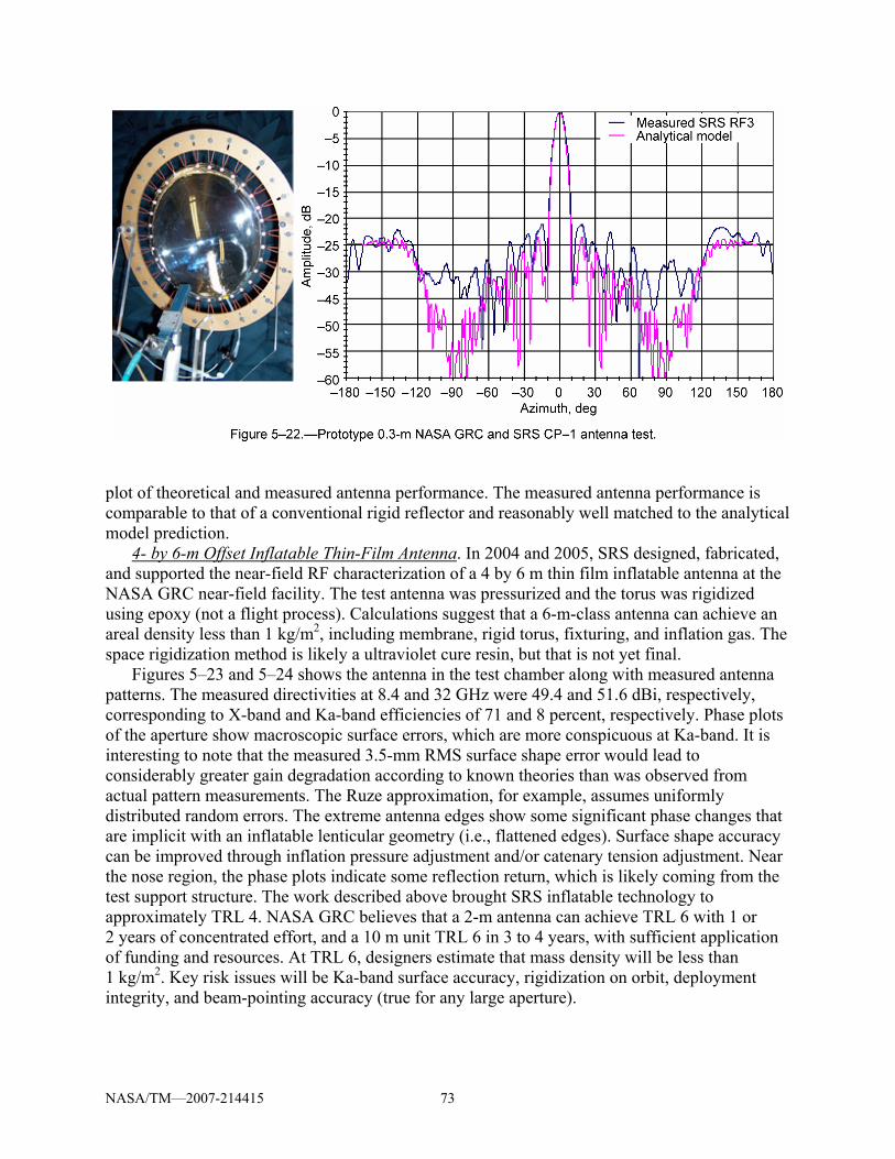
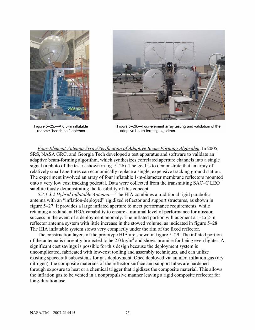
near-field range ......................................................................................................74 Figure 5–24 Measured principal plane patterns of the 4- by 6-m inflatable membrane
reflector at 8.4 GHz. Overall efficiency was 71 percent........................................74 Figure 5–25 A 0.5-m inflatable radome “beach ball” antenna...................................................75 Figure 5–26 Four-element array testing and validation of the adaptive beam-forming
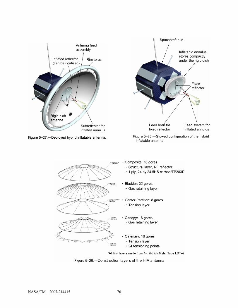
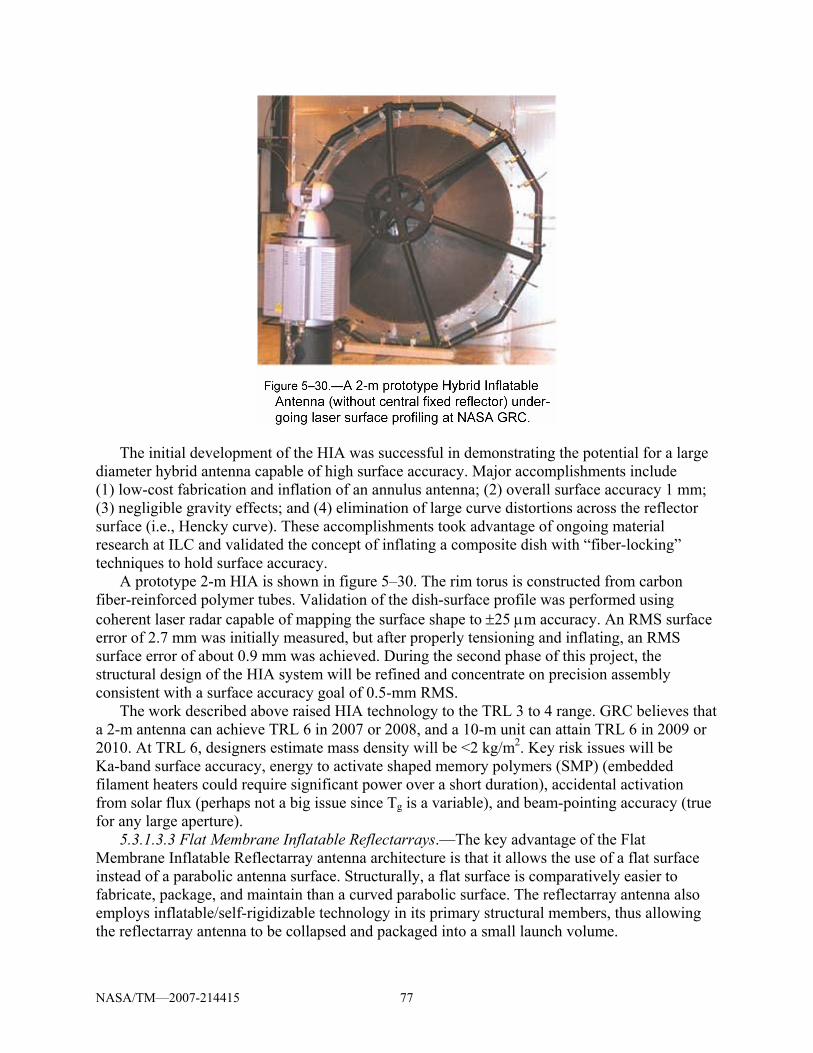
algorithm. ...............................................................................................................75 Figure 5–27 Deployed hybrid inflatable antenna .......................................................................76 Figure 5–28 Stowed configuration of the hybrid inflatable antenna..........................................76 Figure 5–29 Construction layers of the HIA antenna.................................................................76 Figure 5–30 A 2-m prototype Hybrid Inflatable Antenna (without central fixed reflector)
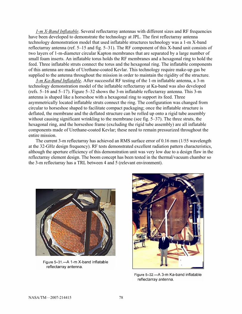
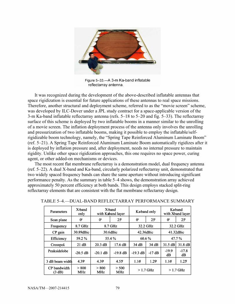
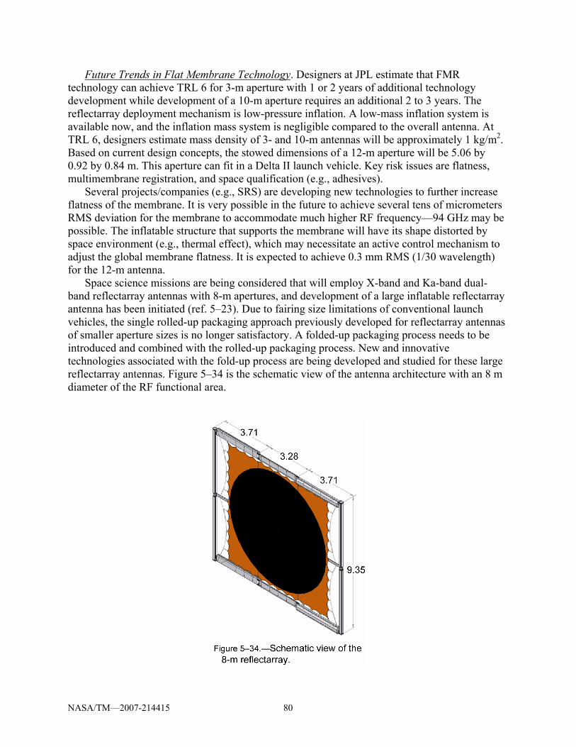
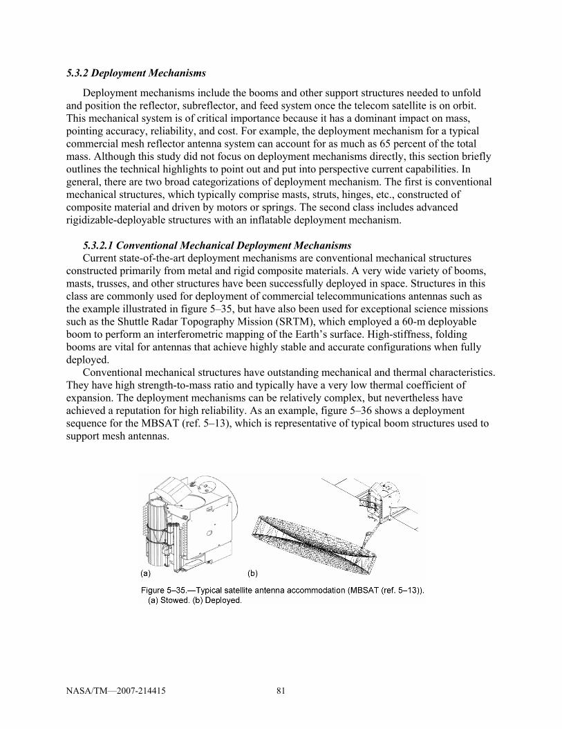
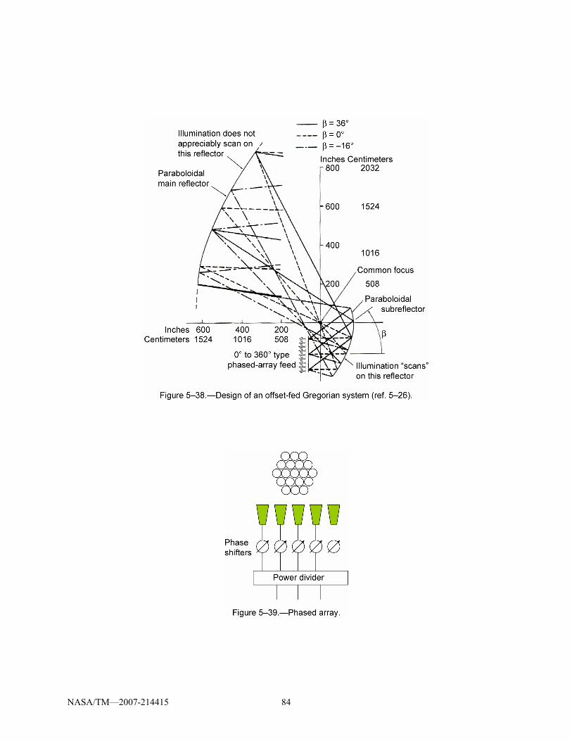
undergoing laser surface profiling at NASA GRC ................................................77 Figure 5–31 A 1-m X-band inflatable reflectarray antenna .......................................................78 Figure 5–32 A 3-m Ka-band inflatable reflectarray antenna .....................................................78 Figure 5–33 A 3-m Ka-band inflatable reflectarray antenna .....................................................79 Figure 5–34 Schematic view of the 8-m reflectarray. ................................................................80 Figure 5–35 Typical satellite antenna accommodation (MBSA (ref. 5–13)). (a) Stowed.
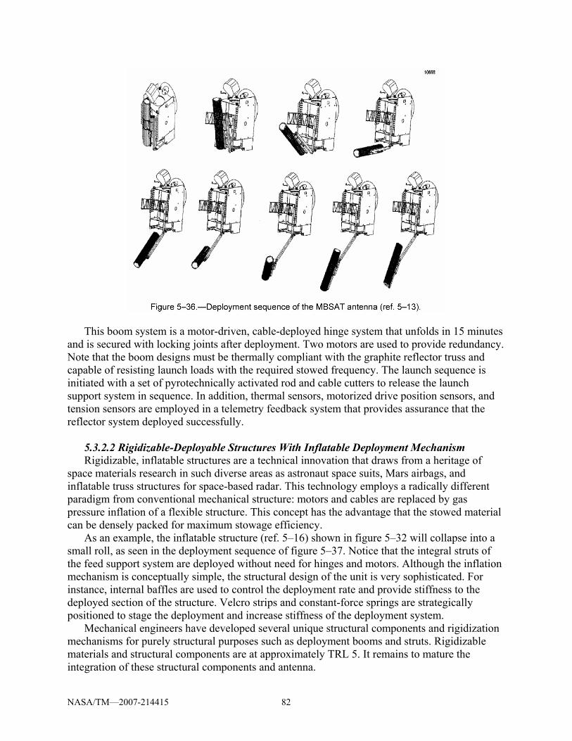
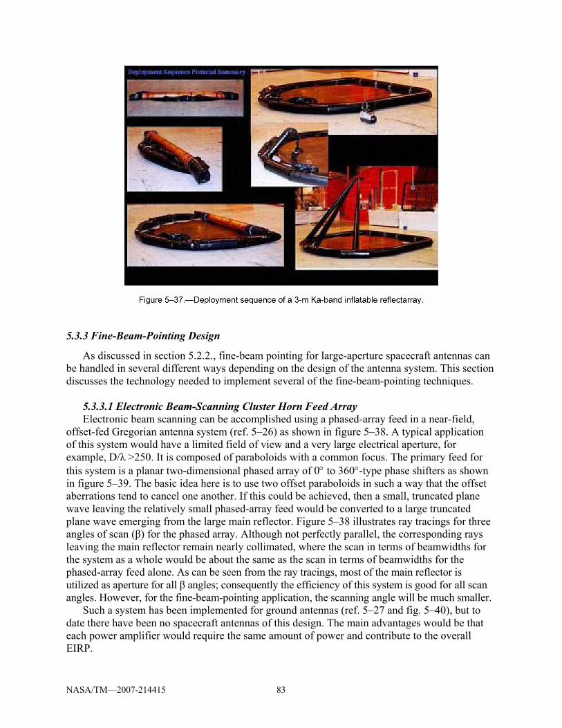
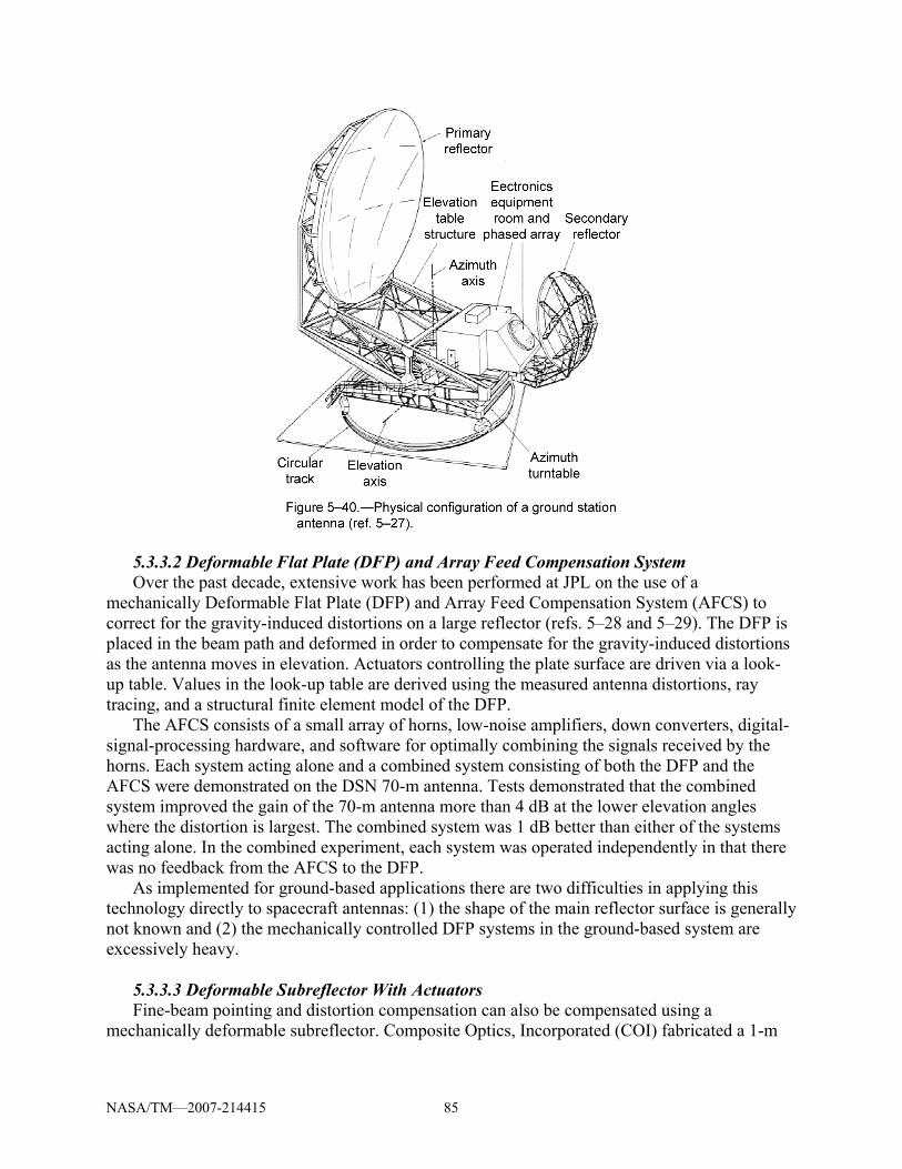
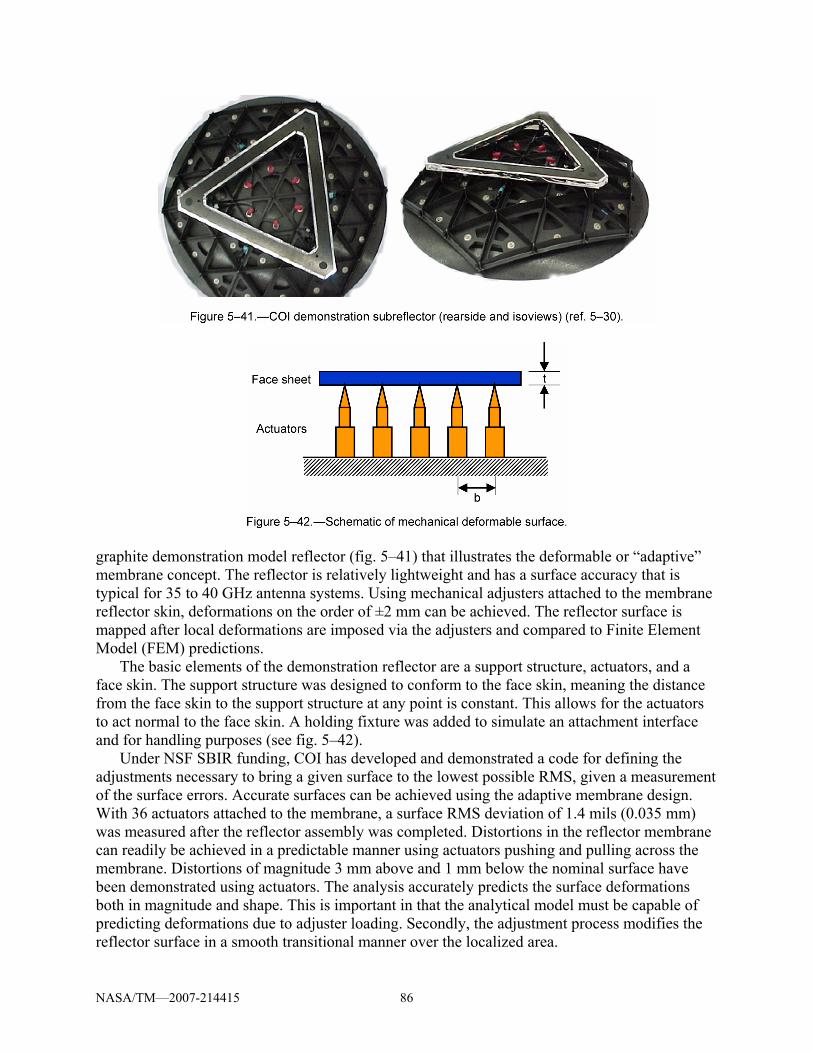
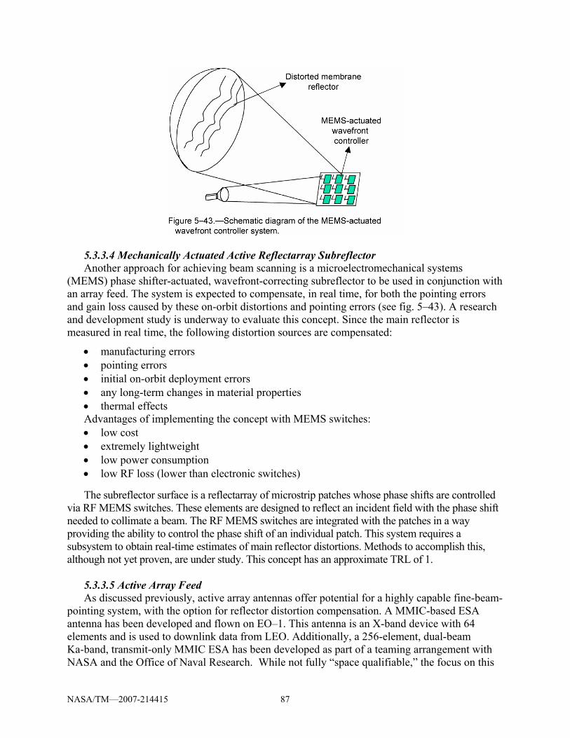
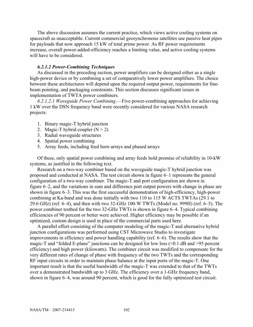
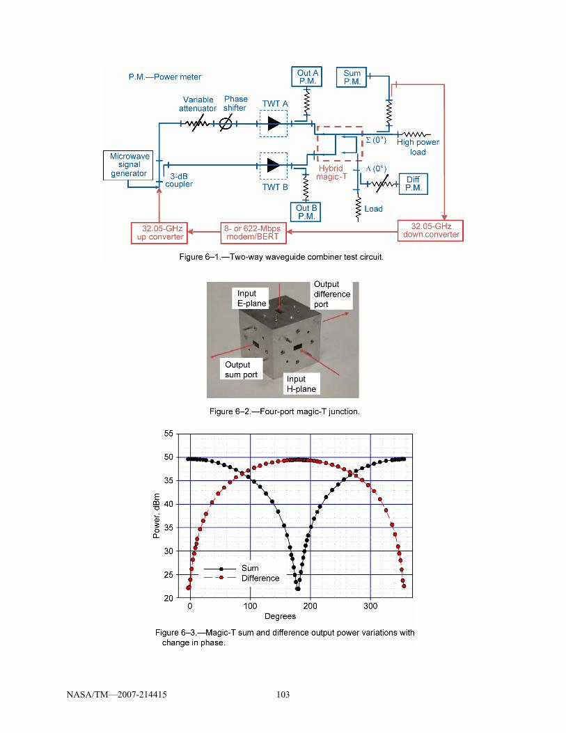
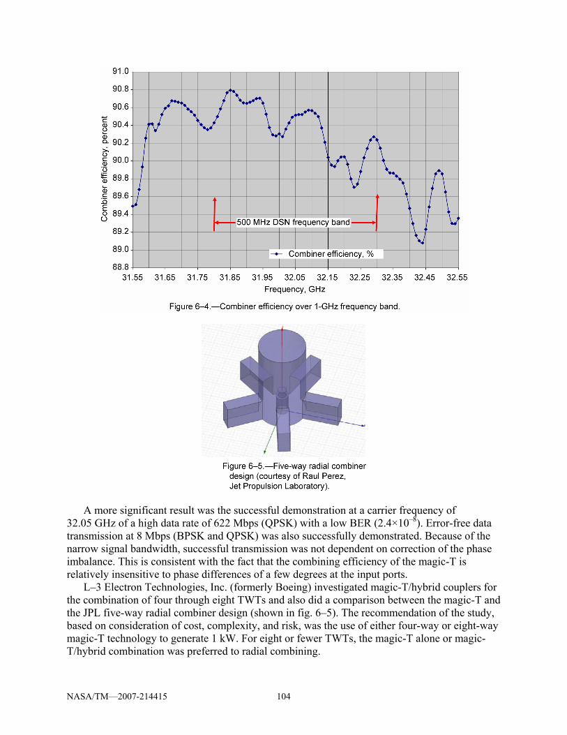
(b) Deployed. .........................................................................................................81 Figure 5–36 Deployment sequence of the MBSAT antenna (ref. 5–13)....................................82 Figure 5–37 Deployment sequence of a 3-m Ka-band inflatable reflectarray ...........................83 Figure 5–38 Design of an offset-fed Gregorian system (ref. 5–26) ...........................................84 Figure 5–39 Phased array ...........................................................................................................84 Figure 5–40 Physical configuration of a ground station antenna (ref. 5–27).............................85 Figure 5–41 COI demonstration subreflector (rearside and isoviews) (ref. 5–30) ....................86 Figure 5–42 Schematic of mechanical deformable surface........................................................86 Figure 5–43 Schematic diagram of the MEMS-actuated wavefront controller system .............87 Figure 6–1 Two-way waveguide combiner test circuit ..........................................................103 Figure 6–2 Four-port magic-T junction..................................................................................103 Figure 6–3 Magic-T sum and difference output power variations with change in phase ......103
NASA/TM—2007-214415 xiii
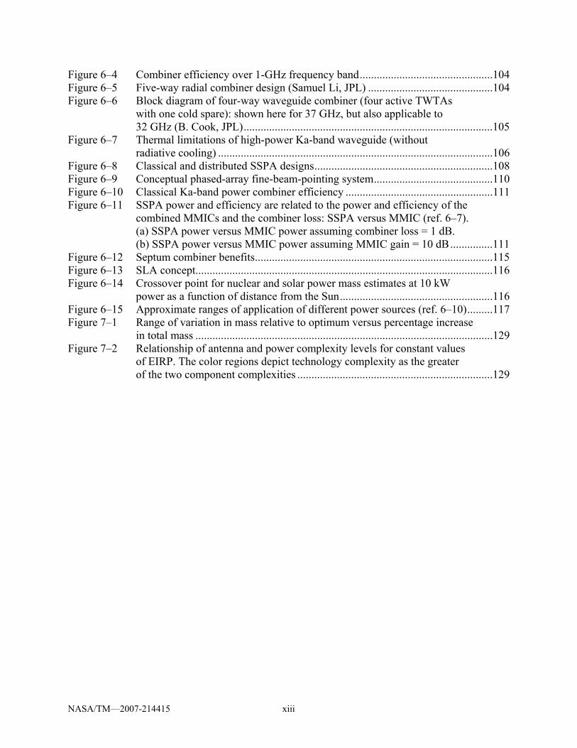
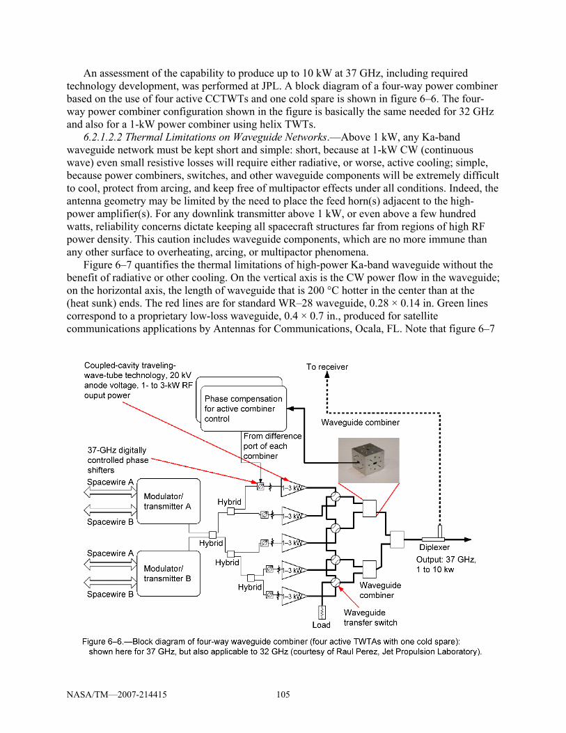
Figure 6–4 Combiner efficiency over 1-GHz frequency band...............................................104 Figure 6–5 Five-way radial combiner design (Samuel Li, JPL) ............................................104 Figure 6–6 Block diagram of four-way waveguide combiner (four active TWTAs
with one cold spare): shown here for 37 GHz, but also applicable to 32 GHz (B. Cook, JPL)........................................................................................105
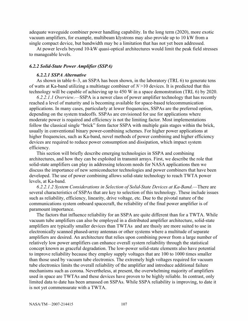
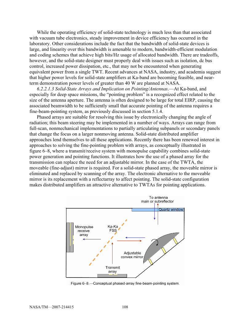
Figure 6–8 Classical and distributed SSPA designs...............................................................108 Figure 6–9 Conceptual phased-array fine-beam-pointing system..........................................110 Figure 6–10 Classical Ka-band power combiner efficiency ....................................................111 Figure 6–11 SSPA power and efficiency are related to the power and efficiency of the
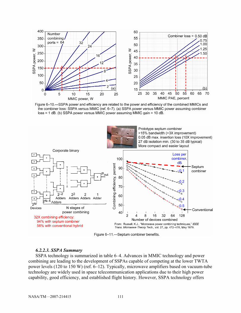
combined MMICs and the combiner loss: SSPA versus MMIC (ref. 6–7). (a) SSPA power versus MMIC power assuming combiner loss = 1 dB. (b) SSPA power versus MMIC power assuming MMIC gain = 10 dB...............111
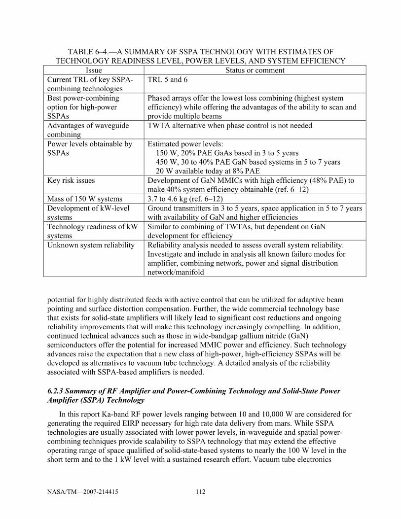
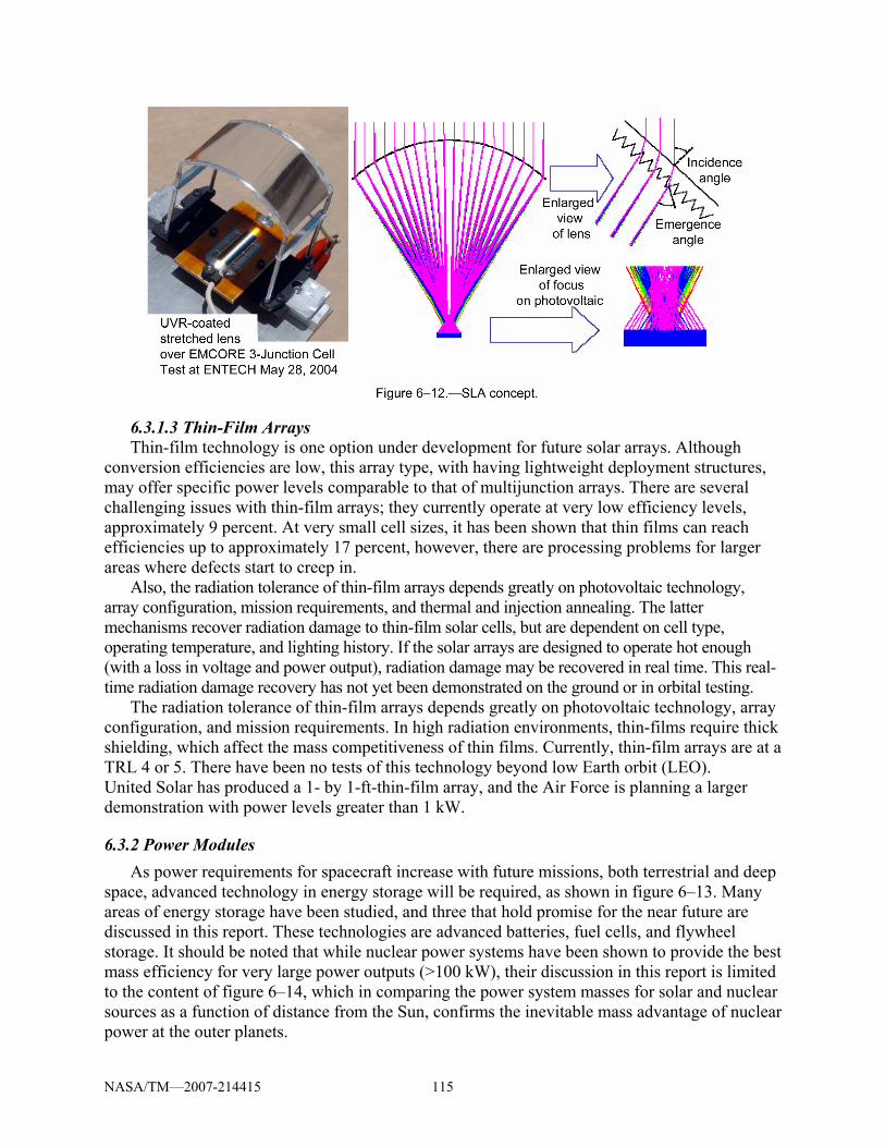
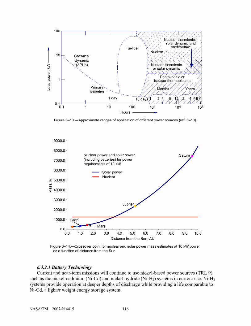
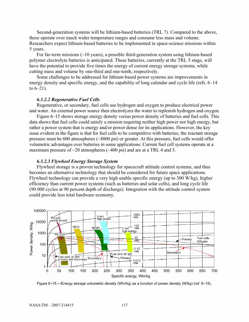
Figure 6–12 Septum combiner benefits....................................................................................115 Figure 6–13 SLA concept.........................................................................................................116 Figure 6–14 Crossover point for nuclear and solar power mass estimates at 10 kW
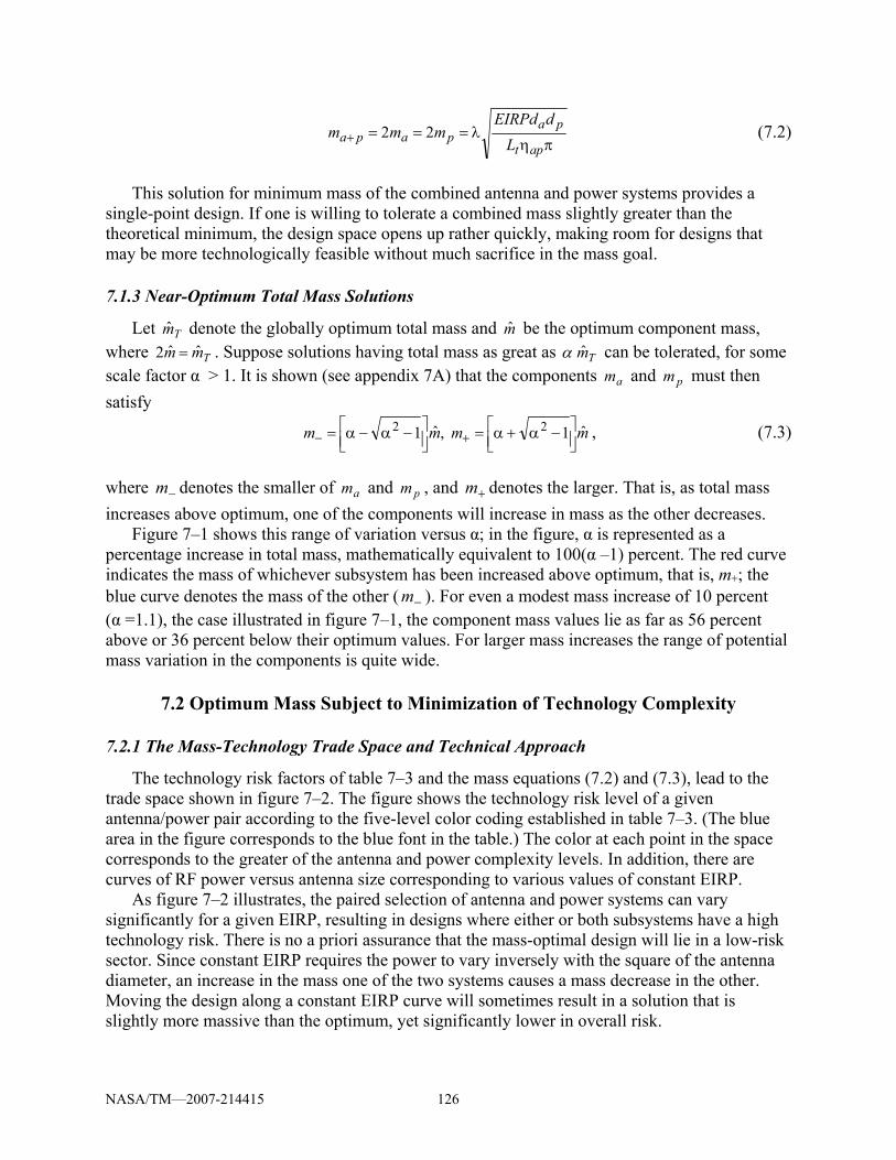
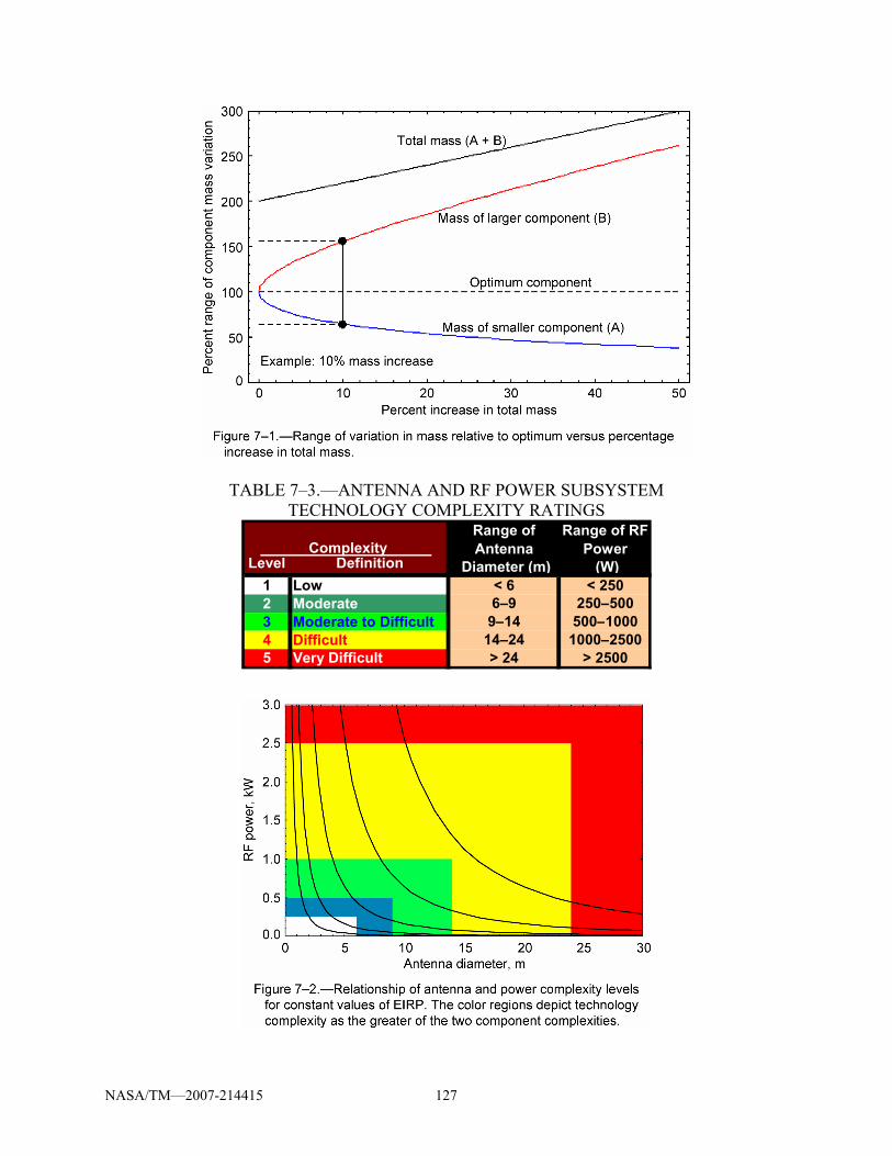
power as a function of distance from the Sun......................................................116 Figure 6–15 Approximate ranges of application of different power sources (ref. 6–10).........117 Figure 7–1 Range of variation in mass relative to optimum versus percentage increase
in total mass .........................................................................................................129 Figure 7–2 Relationship of antenna and power complexity levels for constant values
of EIRP. The color regions depict technology complexity as the greater of the two component complexities .....................................................................129
NASA/TM—2007-214415 1
1. Introduction High-capacity (or high-data-rate) communications is required for human exploration of Mars
and would allow science missions to execute and efficiently complete more data-intensive missions (refs. 1−1 and 1−2). Presently, science missions at Mars operate at very low data rates, such as 120 kbps (kilobits per second) for reporting telemetry from robotic experiments. Not only is this data rate insufficient to meet the expectations of future science missions that are striving to provide the same quality and quantity of return that is achieved on Earth-observing spacecraft, but it also falls short of expectations for activities associated with human exploration.
High-capacity communications over large planetary distances, however, is challenging. This occurs since signal strength, whether optical or radiofrequency (RF), decreases in inverse proportion to the square of the distance, so that getting enough power back to Earth from astronomical unit (AU) distances approaches new technological boundaries. The thesis of this work is that significantly higher capacity communication at RF is possible by utilizing new technology, which will allow increasing the spacecraft effective isotropic radiated power (EIRP) for relatively small increases in spacecraft mass and with reasonable increases in the Earth station effective aperture capabilities. By focusing specifically on the communications return link from Mars to Earth, the challenges and the spacecraft RF technologies that will provide the solutions are presented in the context of a critical piece of NASA’s vision for exploration.
This report will demonstrate that Mars-to-Earth RF communications may achieve data rates as large as 1 Gbps (gigabits per second) with operational systems no later than 2020 using technologies that are at mid-technology readiness level (TRL) 4 to 5 or higher today. These technologies can be developed to TRL 6 or higher by 2020 without excessive monetary expenditures. This is addressed in two segments, the first of which is a discussion of spacecraft telecommunications transmit subsystem designs for a range of data rates (1 Gbps, 500 Mbps, and 100 Mbps) for both a Mars telecom orbiter at maximum Earth-Mars distance and a Crew Exploration Vehicle (CEV) in transit to the Red Planet. Broad recommendations for a CEV communication system will be discussed in the context of investigating how the requirements for an in-transit CEV and those of the transmitting Mars orbiter can simultaneously be met with a prudent allocation of Earth resources. The second segment explores the strategic and high-payoff technology investments that will offer design solutions for RF communications to meet the orbiter and CEV scenarios.
1.1 Approach: Data Rate as Key Parameter
A communications system is designed based on the following five criteria: data rate, bit error rate (BER), end-to-end delay, link availability, and available bandwidth.1 Data rate is the parameter on which this report primarily focuses. Available bandwidth is typically dictated to the designer. The other three, though important, can mostly be addressed in other ways, leaving data rate as the key parameter for an efficient exploration of the RF communications design trade space.
Available bandwidth is of concern in that it will constrain the choices of modulation and coding—and hence the required SNR—for sufficiently high data rates. (Chapter 4 contains some
1Other error measures such as frame or block error rates may be specified, but any such measure ultimately ties back to a BER through the intervening coding and modulation.
NASA/TM—2007-214415 2
discussion of the impact of a Ka-band bandwidth constraint on the data rates that might be achieved as the Earth-Mars distance varies.) Bandwidth-efficient modulation (BEM) and dual polarization are investigated as methods of bits-per-Hertz maximization. However, it should be obvious that the wider the bandwidth the greater the data rate. In this study we assume a 500 MHz bandwidth at 37 GHz. The impact of dual polarizations is to double the bandwidth. If the bandwidth were doubled the data rates discussed could be doubled as well. The hardware is now available to operation over many GHz of bandwidth, allowing operations that encompass the 32- and 37-GHz bands with the same hardware. We mention this here because it is important, but we do not attempt to work the bandwidth topic in this document.
For completeness the other three criteria are briefly described: (1) The link availability is determined by the architecture selected and is based on orbital mechanics and, where applicable, planetary weather conditions. The acceptable availability will be specified by the mission designers. (2) The end-to-end delay is determined predominantly by the light travel time. From Mars to Earth the delay may be from 3 to 22 min depending on distance. (3) The BER is determined by modulation, coding, and the available bit signal-to-noise ratio (SNR) at the receiver. The analysis contained in this report includes sufficient received signal strength to permit low BER (see appendix 4A for referenced link budget used in this report), and the issue is not addressed in any further detail.
Therefore while BER, delay, and availability are important, they will not be discussed, at length, in this report. Instead this effort will focus on Mars-to-Earth data rates as large as 1 Gbps, with emphasis on data rates and their implications, as opposed to the other parameters associated with communication systems. Chapter 2 will describe in more detail the surface robotic and human exploration scenarios as well as the Crew Exploration Vehicle (CEV)-to-Mars transit scenario that provide the rationale for the data rate selection and ranges used in the remainder of the report. Chapter 3 introduces the technical assumptions for the link design as preparation for chapter 4, which delves into the RF design trade space parameters of spacecraft subsystem mass and power as well as features of the Earth receive system. The capabilities in the spacecraft and on Earth at a distance of 2.67 AU are investigated: three different data rates (1 Gbps and 500 and 100 Mbps) for the relay and 1 Mbps for the CEV. Fixing the required resources to achieve the desired data rates at 2.67 AU means that greater data rates can be achieved for the CEV in transit (tens of Mbps) and for the relay in its orbit (a few Gbps). Chapters 5 and 6 provide a technical review of the primary technologies that enable high-capacity communications: antenna and power systems. Finally, chapter 7 integrates the design and technology aspects to evaluate approaches for mass minimization and assessing the associated technical complexity. Chapter 8 provides a summary of the results and highlights the conclusions of the work.
1.2 Background and Challenges of Spacecraft RF Design
1.2.1 Mass and Power
Those participating in the space community are all too familiar with the dynamic between mass, power, and cost in the design of a spacecraft. The communications subsystem is no exception; not only must a fine balance between communications system mass and power be found, but the design of the subsystem must be taken in context with the complete spacecraft and the total mass and power budgets.
The two primary contributions to spacecraft mass and power from the communications subsystem are the RF power subsystem and the transmit antenna. The RF transmitter is
NASA/TM—2007-214415 3
characterized by its rated power, efficiency, and bandwidth, while the antenna is characterized by its throwing power or EIRP (effective isotropic radiated power). The EIRP is directly proportional to the antenna area and efficiency. Chapters 5 and 6 address candidate technologies for spacecraft antennas and transmitters, respectively. The description of power generating systems is also included in chapter 6. Since the achievable data rate is proportional to the transmit EIRP, both a large spacecraft antenna and a high-power transmit amplifier will be required for the highest data rates. Therefore an optimal communications system design will include a large spacecraft antenna, high-power transmitters, and robust surface receive system.
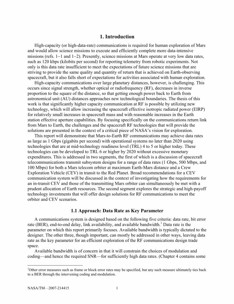
Examples of the relationship between the communications subsystem and the full spacecraft are provided by recent Mars missions such as the Mars Reconnaissance Orbiter (MRO) and Mars Global Surveyor (MGS). MRO, launched in 2005, has a Ka-band transmitter, a 35-W Ka-band traveling-wave-tube amplifier (TWTA), and spacecraft antenna of 3 m that will provide 6 Mbps coded at Mars (min. range) by December 2007 into a single 34-m Deep Space Network (DSN) antenna at Goldstone.2 Spacecraft designers have typically not allocated very much mass and power to the communications equipment. As shown in and, for example, in Mars Global Surveyor the communications payload is the next to smallest subsystem in mass.
TABLE 1–1.—ACTUAL VALUES ASSOCIATED WITH THE SUBSYSTEMS
Subsystem Mars Global Surveyor subsystem mass, kg
Power 135 Structures 95 Command and DH 83 Science Payload 75 Propulsion 75 Cabling 70 ACS 60 Telecom—includes all communications 55 Thermal 15
2The other two sites will be at lower data rates due to elevation and weather issues, but this shows the possibility of much higher rates. For example if a 3.5-kW TWTA were used, the rate could be 100 times larger.
NASA/TM—2007-214415 4
In comparing the data from various spacecraft, the communications subsystem package remains one of the smallest in mass. Therefore it becomes obvious that much larger data rates could be obtained if more mass were allocated to the communications systems. In this document, we are proposing to increase the telecom mass to about one and one-half or more of the mass for MGS (55 kg). This increase would allow for dramatic increases in data rates.
1.2.2 The Mars-Earth Dynamic
Some of the communications challenges result from the orbital geometry between Mars and the Earth. The variable distance has significant impact on the achievable data rate, the geometry imposes pointing requirements on the spacecraft, and the combination of geometry and thermal environment impacts the design of the antenna.
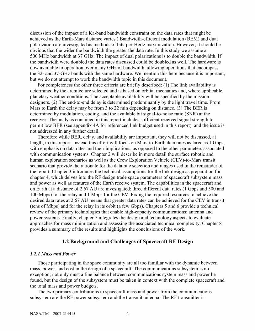
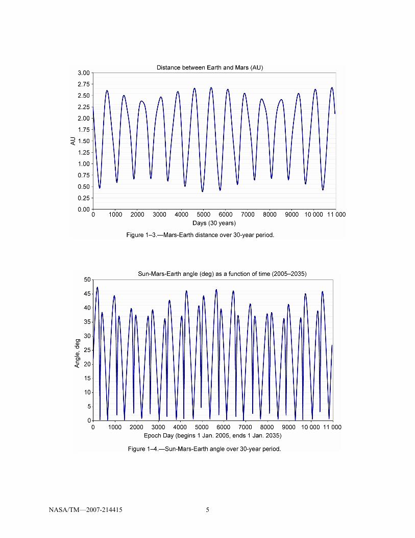
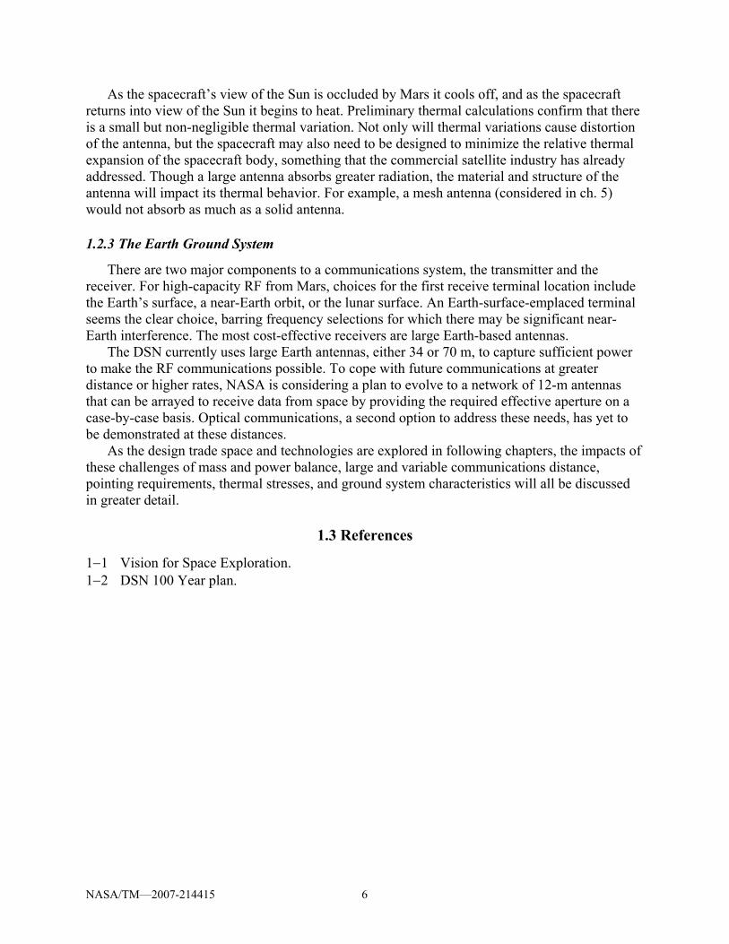
The light travel time from Mars to Earth varies by a factor of 7 depending on the distance between the two planets. That distance may be as small as 0.38 AU or as large as 2.67 AU over the next 25 years. The mean distance is 1.70 AU. Figure 1−3 shows the Mars-Earth distance over 30-year period and figure 1−4 shows the Sun-Mars-Earth angle over the same 30-year period. The large variation in distance has significant impact on the data rate available from the spacecraft, as discussed in a later chapter. A Mars-orbiting satellite for relaying communications from the planet would need sizable, but reasonable, communication assets to deliver power to the surface of the Earth sufficient to enable a data rate of 1 Gbps at maximum range.
The Mars relay satellite will continually point its antenna towards Earth during each revolution around Mars. Over a period of a Martian year, the Earth will move around the Sun, presenting a ±45° angle on each side of the Sun as viewed from Mars. As the spacecraft orbits Mars, it will point in the same direction, that is, the spacecraft will have inertial pointing. Nevertheless, a mechanism to maintain pointing finer tolerances than that normally provided by spacecraft Attitude Determination and Control System (ADCS). To maintain a low antenna pointing loss the spacecraft must be pointed with small error. Large antennas exacerbate the problem; they have smaller beam divergence angles, therefore, pointing loss becomes more sensitive to pointing error as the diameter increases. Details of fine-pointing mechanisms are discussed in chapter 5.
NASA/TM—2007-214415 5
NASA/TM—2007-214415 6
As the spacecraft’s view of the Sun is occluded by Mars it cools off, and as the spacecraft returns into view of the Sun it begins to heat. Preliminary thermal calculations confirm that there is a small but non-negligible thermal variation. Not only will thermal variations cause distortion of the antenna, but the spacecraft may also need to be designed to minimize the relative thermal expansion of the spacecraft body, something that the commercial satellite industry has already addressed. Though a large antenna absorbs greater radiation, the material and structure of the antenna will impact its thermal behavior. For example, a mesh antenna (considered in ch. 5) would not absorb as much as a solid antenna.
1.2.3 The Earth Ground System
There are two major components to a communications system, the transmitter and the receiver. For high-capacity RF from Mars, choices for the first receive terminal location include the Earth’s surface, a near-Earth orbit, or the lunar surface. An Earth-surface-emplaced terminal seems the clear choice, barring frequency selections for which there may be significant near-Earth interference. The most cost-effective receivers are large Earth-based antennas.
The DSN currently uses large Earth antennas, either 34 or 70 m, to capture sufficient power to make the RF communications possible. To cope with future communications at greater distance or higher rates, NASA is considering a plan to evolve to a network of 12-m antennas that can be arrayed to receive data from space by providing the required effective aperture on a case-by-case basis. Optical communications, a second option to address these needs, has yet to be demonstrated at these distances.
As the design trade space and technologies are explored in following chapters, the impacts of these challenges of mass and power balance, large and variable communications distance, pointing requirements, thermal stresses, and ground system characteristics will all be discussed in greater detail.
1.3 References
1−1 Vision for Space Exploration. 1−2 DSN 100 Year plan.
NASA/TM—2007-214415 7
2. Assumed Design Scenarios This chapter begins by describing an assumed communication scenario for human and
robotic exploration of Mars. It is followed by a scenario relating to the CEV that will carry humans to and from Mars. These two scenarios capture the key aspects of communication needs for Mars mission support.
2.1 Scenarios for Mars Exploration
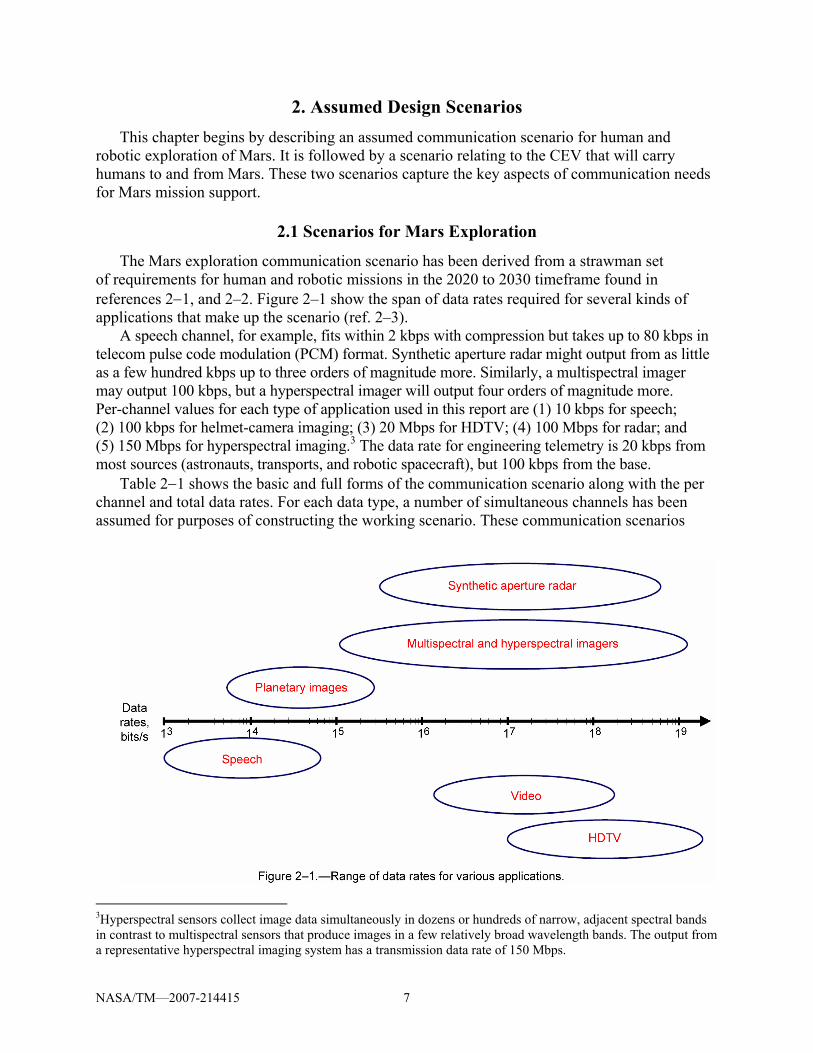
The Mars exploration communication scenario has been derived from a strawman set of requirements for human and robotic missions in the 2020 to 2030 timeframe found in references 2−1, and 2–2. Figure 2–1 show the span of data rates required for several kinds of applications that make up the scenario (ref. 2–3).
A speech channel, for example, fits within 2 kbps with compression but takes up to 80 kbps in telecom pulse code modulation (PCM) format. Synthetic aperture radar might output from as little as a few hundred kbps up to three orders of magnitude more. Similarly, a multispectral imager may output 100 kbps, but a hyperspectral imager will output four orders of magnitude more. Per-channel values for each type of application used in this report are (1) 10 kbps for speech; (2) 100 kbps for helmet-camera imaging; (3) 20 Mbps for HDTV; (4) 100 Mbps for radar; and (5) 150 Mbps for hyperspectral imaging.3 The data rate for engineering telemetry is 20 kbps from most sources (astronauts, transports, and robotic spacecraft), but 100 kbps from the base.
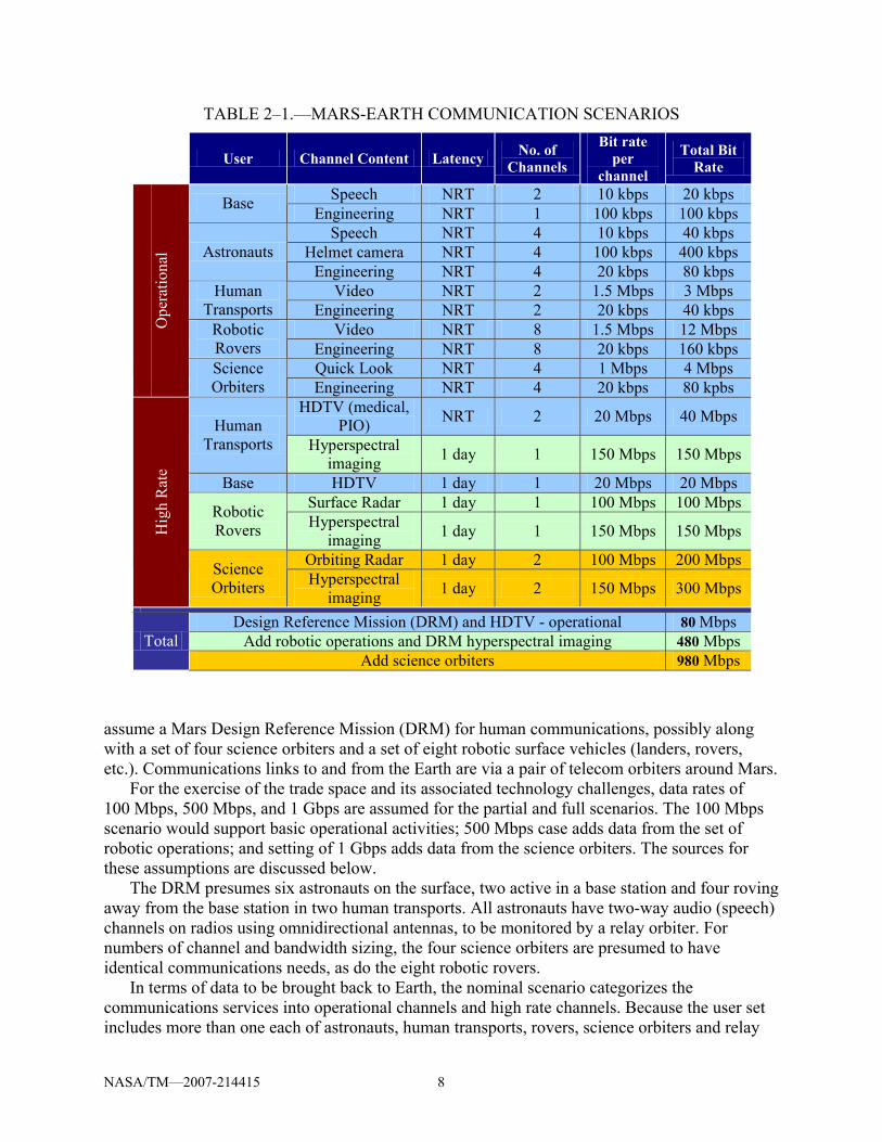
Table 2−1 shows the basic and full forms of the communication scenario along with the per channel and total data rates. For each data type, a number of simultaneous channels has been assumed for purposes of constructing the working scenario. These communication scenarios
3Hyperspectral sensors collect image data simultaneously in dozens or hundreds of narrow, adjacent spectral bands in contrast to multispectral sensors that produce images in a few relatively broad wavelength bands. The output from a representative hyperspectral imaging system has a transmission data rate of 150 Mbps.
Transports Hyperspectral imaging 1 day 1 150 Mbps 150 Mbps
Base HDTV 1 day 1 20 Mbps 20 Mbps Surface Radar 1 day 1 100 Mbps 100 Mbps Robotic
Rovers Hyperspectral imaging 1 day 1 150 Mbps 150 Mbps
Orbiting Radar 1 day 2 100 Mbps 200 Mbps
Hig
h R
ate
Science Orbiters Hyperspectral
imaging 1 day 2 150 Mbps 300 Mbps
Design Reference Mission (DRM) and HDTV - operational 80 Mbps Add robotic operations and DRM hyperspectral imaging 480 Mbps Total
Add science orbiters 980 Mbps
assume a Mars Design Reference Mission (DRM) for human communications, possibly along with a set of four science orbiters and a set of eight robotic surface vehicles (landers, rovers, etc.). Communications links to and from the Earth are via a pair of telecom orbiters around Mars.
For the exercise of the trade space and its associated technology challenges, data rates of 100 Mbps, 500 Mbps, and 1 Gbps are assumed for the partial and full scenarios. The 100 Mbps scenario would support basic operational activities; 500 Mbps case adds data from the set of robotic operations; and setting of 1 Gbps adds data from the science orbiters. The sources for these assumptions are discussed below.
The DRM presumes six astronauts on the surface, two active in a base station and four roving away from the base station in two human transports. All astronauts have two-way audio (speech) channels on radios using omnidirectional antennas, to be monitored by a relay orbiter. For numbers of channel and bandwidth sizing, the four science orbiters are presumed to have identical communications needs, as do the eight robotic rovers.
In terms of data to be brought back to Earth, the nominal scenario categorizes the communications services into operational channels and high rate channels. Because the user set includes more than one each of astronauts, human transports, rovers, science orbiters and relay
NASA/TM—2007-214415 9
orbiters, there are as many channels of each type as instances of the user type. For example, the scenario sums to six speech channels of 10 kbps each for six astronauts.
Human communication would be sporadic but would require near-real-time (NRT) communication with high link availability. The continuity of robotic exploration would likewise require NRT and high availability for operational data, while its science would be non-real-time and high rate (volume). The scenario includes several operational and high rate services, each specifying its own quality of service (QoS).
Channels can be further categorized into four classes: emergency, operational, Public Information Office, and high volume.
• Emergency: a real-time channel requiring continuous, low-rate communication at
unpredictable times and of unpredictable duration • Operational: high availability, NRT communication needed for day-to-day operation;
near 100 percent completeness on first transmission. • Public Information Office: high reliability, NRT high-definition television (HDTV), with
low frame error rate • High volume: non-real-time, relatively low availability and relatively high frame error
rate; use as yet undetermined networking protocols to accommodate goals of delay minimization and almost error-free transmission.
At the bottom of the table the scenario is parsed into three gradations. The basic form of the
scenario consists mostly of operational data from the human and robotic missions, and these channels sum to about 80 Mbps. Most of the basic data is required in NRT, as limited by the communications time between Earth and Mars. The changing distance between Earth and Mars results in a variation in the communications time from 3 to 22 minutes (one way) at minimum and maximum distances, respectively. From a monitor and control perspective with Earth in the loop, two-way light time varies from 6 to 44 minutes. If an astronaut asks a question of Mission Control when at maximum range from Earth, it will be at least 44 minutes before the astronaut can hear a reply.
An intermediate stepup in the scenario results when robotic operations and some hyperspectral imaging are introduced. The total data rate would peak at ~500 Mbps though unlikely, all these sources transmitted simultaneously.
The full scenario adds radar and hyperspectral imaging to the robotic rovers and science orbiters. These, together with the scenario 1 channels, sum to about 980 Mbps. Although the full scenario also requires NRT availability for operational communication, the radar and imaging channels are not on 24 hours a day. It is clear that the instantaneous data rate for the full scenario could be substantially less than 1 Gbps most of the time. It should also be pointed out that it is very difficult to predict data needs for the year 2030. For example, three-dimensional video transmissions may require twice the rate stated in these scenarios. In this section we have made an attempt to review various user sources and provide possible bandwidth allocations based on the assumed scenarios. It is likely that the actual scenarios will be different than the assumptions made here. The goal has been to capture the possible bandwidth requirements such that even if the scenarios change, the bandwidth allocation can still support the scenarios.
In summary, data rates of 1 Gbps, 500 Mbps, and 100 Mbps are assumed in the analysis that paves the way for identifying the technology needs for high-rate Mars-to-Earth communications.
NASA/TM—2007-214415 10
2.2 CEV Communication Scenario
Inclusion of the CEV in the overall discussion of Mars-to-Earth communications is significant. Certainly the CEV and Mars relay communication systems will not be designed without regard for one another, and in fact one may expect the two systems to share resources on Earth. At present it is hard to imagine any rationale for the CEV using optical communications to close its links to Earth. That being the case, the use of RF in a manner compatible with the future receive array seems warranted for both platforms. (Resource sharing is investigated in ch. 7.)
The data rates required for the CEV at Mars distances have not yet been determined, but can be expected to be well less that required of a Mars relay. At least one scenario for communications for the CEV would include a large data rate (~150 Mbps) from near Earth, decreasing as the CEV approached Mars vicinity. Once in contact with a Mars communications relay, the data rates from CEV could be increased significantly by the use of the relay capability near Mars.
The communication system for Mars missions must support the CEV in transit at all intermediate distances. The current best estimate of CEV communication requirements at Ka-band is that the in-transit (State 1) vehicle must be able to return up to 1 Mbps via direct link to the DSN array at Earth. In Mars orbit (State 2) the data return capability is to be tens of Mbps, in which case the vehicle can be supported by a Mars relay.
The present goal is that the Ka-band RF components on the CEV be limited to no more than 1 m antenna diameter and 100-W RF output power. The size restriction stems from the fact that the antenna will have to be gimbaled to achieve the range of pointing angles required for the various regions of operation. In addition, larger antennas may cause visual blockage problems for the crew. The present goal is that the Ka-band RF components be limited to no more than 1 m antenna diameter and 100-W RF output power. The size restriction stems from the fact that the antenna will have to be gimbaled to achieve the range of pointing angles required for the various regions of operation. In addition, larger antennas may cause visual blockage problems for the crew.
Chapter 7 of this report has as its prime objective an examination, for a Mars relay satellite, of the technology trades among spacecraft antenna size, RF output power, and ground array network from a technology risk mitigation viewpoint. Once some designs are found that offer a stipulated performance and simultaneously minimize the level of relay satellite technology complexity, the impact on the Earth-based array network can be readily derived. As a follow-up, it is interesting to see whether these derived requirements for the array are also adequate to provide the cited level of CEV support. This analysis is reported in section 7.3.
2.3 References
2−1 SCAWG RF Sub Team: Deep Space RF Trade Study Initial Report (Draft). Feb. 2005. 2−2 SCAWG RF Sub Team: Deep Space RF Trade Study Report.” Mar. 2005. 2−3 Noreen, G. et al.: Integrated Network Architecture for Sustained Human and Robotic
Exploration.” 2005 IEEE Aerospace Conference, Big Sky, Montana, Mar. 5, 2005, updated Dec. 28, 2004.
NASA/TM—2007-214415 11
3. Assumptions for Mars RF Link Design High-rate communications from Mars has significant but manageable challenges during the
timeline 2020 to 2030. MRO sends data on X-band at rates as high as 5.3 Mbps. MRO could have been designed to send data at much higher rates than 5.3 Mbps over most Mars-Earth distances were it not for bandwidth limitations at X-band (ref. 3−1).
The bandwidth issue is less severe at Ka-band. The deep space allocation for Ka-band is 500 MHz, compared with 50 MHz at X-band. This section discusses the various assumptions and challenges foreseen for a high rate Ka-band downlink. These assumptions and challenges include spacecraft constraints, ground station configuration, weather and atmospheric implications, solar conjunction, spectrum constraints, and the extreme variation in Earth-Mars distance.
3.1 Spacecraft Constraints
High-rate communications from Mars requires developing RF technology capability with high availability, reliability, and increased bandwidth. The high rate will result in the use of large antennas along with high-power transmitters. The requirement for generating a specific effective EIRP is a function of a trade between the Earth station G/T (antenna gain to operating temperature ratio) and the spacecraft power/gain parameters. Some of the spacecraft assumptions to be used for design and analysis, based on the ongoing technology research discussed in chapters 5 and 6, are the following:
• Power amplifier RF output levels range from 0.2 to 2.5Kw • Antenna diameters range from 4 to 25 m. Antennas below 12 m are assumed to be
pointed with the spacecraft ACS, while larger antennas would require a fine-pointing mechanism.
• A worst-case pointing error loss of 1 dB and a worst-case pointing ability of 14 mdeg (coarse pointing) are required. This assumes the high-gain antenna (HGA) pointing to Earth is body mounted and depends on the spacecraft ACS for antenna pointing accuracy.
• The spacecraft antenna for the link to Earth always points at Earth, implying that the antenna for proximity communications will require a gimbaled mechanism. Proximity communications and antennas are not covered here and will need to be visited in the future.
Other issues and concerns, addressed in chapters 5 and 6, include the availability of • space-qualifiable RF components operating at high power levels with low mass and good
power conversion efficiency • Ka-band antennas with good efficiency • deployment mechanisms for large antennas
NASA/TM—2007-214415 12
3.2 Ground Network
The ground network assumed for the Mars-to-Earth communications links is the future DSN ground network array, composed of multiple 12-m antennas, along with the associated electronics and control systems, at each of three sites. For comparison, this section also provides the capabilities of the existing (2005) DSN with its 34- and 70-m antennas.
The DSN plans to develop an initial array with 12 elements for demonstration by midcalendar year 2007 and will operationally deploy the array at each of the DSN sites with as many elements as is required starting in mid-2010. With respect to supporting the Mars relay, however, a trade space will be investigated in which the DSN array at three sites is assumed for this service, starting around the year 2020.
The telecommunications link between the Earth and spacecraft engaged in solar system exploration at Mars includes the DSN. This network currently consists of large antennas spaced approximately equally in longitude around the Earth (ref. 3−2). The current DSN has a few large antennas at each of three longitudes (sites): Goldstone, California, U.S.A.; Madrid, Spain; and Canberra, Australia. Each site includes one 70-m Cassegrain antenna, one 34-m high-efficiency (HEF) antenna, and from one to three 34-m beam-waveguide (BWG) antennas.
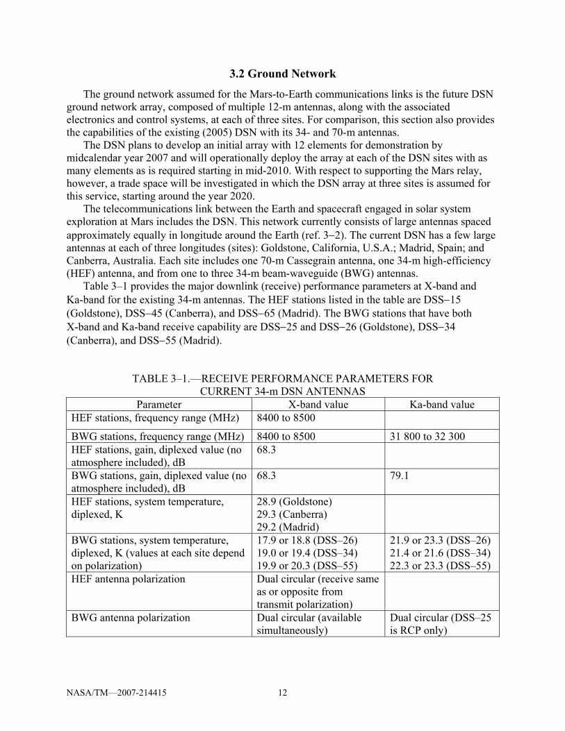
Table 3–1 provides the major downlink (receive) performance parameters at X-band and Ka-band for the existing 34-m antennas. The HEF stations listed in the table are DSS−15 (Goldstone), DSS−45 (Canberra), and DSS−65 (Madrid). The BWG stations that have both X-band and Ka-band receive capability are DSS−25 and DSS−26 (Goldstone), DSS−34 (Canberra), and DSS−55 (Madrid).
TABLE 3–1.—RECEIVE PERFORMANCE PARAMETERS FOR CURRENT 34-m DSN ANTENNAS
Parameter X-band value Ka-band value HEF stations, frequency range (MHz) 8400 to 8500
BWG stations, frequency range (MHz) 8400 to 8500 31 800 to 32 300 HEF stations, gain, diplexed value (no atmosphere included), dB
68.3
BWG stations, gain, diplexed value (no atmosphere included), dB
68.3 79.1
HEF stations, system temperature, diplexed, K
28.9 (Goldstone) 29.3 (Canberra) 29.2 (Madrid)
BWG stations, system temperature, diplexed, K (values at each site depend on polarization)
17.9 or 18.8 (DSS–26) 19.0 or 19.4 (DSS–34) 19.9 or 20.3 (DSS–55)
21.9 or 23.3 (DSS–26) 21.4 or 21.6 (DSS–34) 22.3 or 23.3 (DSS–55)
HEF antenna polarization Dual circular (receive same as or opposite from transmit polarization)
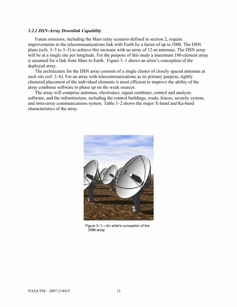
Future missions, including the Mars relay scenario defined in section 2, require improvements in the telecommunications link with Earth by a factor of up to 1000. The DSN plans (refs. 3–3 to 3–5) to achieve this increase with an array of 12-m antennas. The DSN array will be at a single site per longitude. For the purpose of this study a maximum 180-element array is assumed for a link from Mars to Earth. Figure 3–1 shows an artist’s conception of the deployed array.
The architecture for the DSN array consists of a single cluster of closely spaced antennas at each site (ref. 3–6). For an array with telecommunications as its primary purpose, tightly clustered placement of the individual elements is most efficient to improve the ability of the array combiner software to phase up on the weak sources.
The array will comprise antennas, electronics, signal combiner, control and analysis software, and the infrastructure, including the control buildings, roads, fences, security system, and intra-array communications system. Table 3–2 shows the major X-band and Ka-band characteristics of the array.
NASA/TM—2007-214415 14
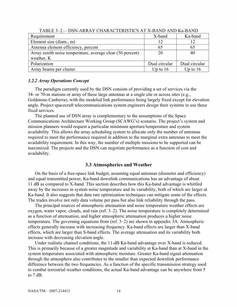
TABLE 3–2.—DSN-ARRAY CHARACTERISTICS AT X-BAND AND Ka-BAND Requirement X-band Ka-band Element size (diam., m) 12 12 Antenna element efficiency, percent 65 65 Array zenith noise temperature, average clear (50 percent) weather, K
20 40
Polarization Dual circular Dual circular Array beams per cluster Up to 16 Up to 16
3.2.2 Array Operations Concept
The paradigm currently used by the DSN consists of providing a set of services via the 34- or 70-m stations or array of these large antennas at a single site or across sites (e.g., Goldstone-Canberra), with the modeled link performance being largely fixed except for elevation angle. Project spacecraft telecommunications system engineers design their systems to use these fixed services.
The planned use of DSN array is complementary to the assumptions of the Space Communications Architecture Working Group (SCAWG’s) scenario. The project’s system and mission planners would request a particular minimum aperture/temperature and system availability. This allows the array scheduling system to allocate only the number of antennas required to meet the performance required in addition to the marginal extra antennas to meet the availability requirement. In this way, the number of multiple missions to be supported can be maximized. The projects and the DSN can negotiate performance as a function of cost and availability.
3.3 Atmospherics and Weather
On the basis of a free-space link budget, assuming equal antennas (diameter and efficiency) and equal transmitted power, Ka-band downlink communications has an advantage of about 11 dB as compared to X-band. This section describes how this Ka-band advantage is whittled away by the increases in system noise temperature and its variability, both of which are larger at Ka-band. It also suggests that data rate optimization techniques can mitigate some of the effects. The trades involve not only data volume per pass but also link reliability through the pass.
The principal sources of atmospheric attenuation and noise temperature weather effects are oxygen, water vapor, clouds, and rain (ref. 3–2). The noise temperature is completely determined as a function of attenuation, and higher atmospheric attenuation produces a higher noise temperature. The governing equations from (ref. 3–2) are shown in appendix 3A. Atmospheric effects generally increase with increasing frequency. Ka-band effects are larger than X-band effects, which are larger than S-band effects. The average attenuation and its variability both increase with decreasing elevation angle.
Under realistic channel conditions, the 11-dB Ka-band advantage over X-band is reduced. This is primarily because of a greater magnitude and variability at Ka-band than at X-band in the system temperature associated with atmospheric moisture. Greater Ka-band signal attenuation through the atmosphere also contributes to the smaller than expected downlink performance difference between the two frequencies. As a function of the specific transmission strategy used to combat terrestrial weather conditions, the actual Ka-band advantage can be anywhere from 5 to 7 dB.
NASA/TM—2007-214415 15
Atmospheric noise temperature and attenuation affect link reliability since an outage occurs whenever an elevated noise temperature and increased attenuation cause the SNR to fall below the threshold.
Tables 3–3 and 3–4 show Ka-band and X-band noise temperatures and atmospheric attenuations (refs. 3–2, 3–7, and 3–8). The tables are organized to show atmospheric effects in terms of “90 percent weather,” “95 percent weather,” and “99 percent weather.” These terms mean that the noise temperature and attenuation exceed the tabulated values only 10, 5, or 1 percent of the time, respectively.
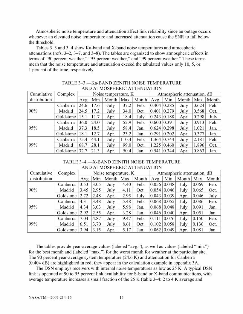
TABLE 3–3.––Ka-BAND ZENITH NOISE TEMPERATURE
AND ATMOSPHERIC ATTENUATION Noise temperature, K Atmospheric attenuation, dB Cumulative
distribution Complex
Avg. Min. Month Max. Month Avg. Min. Month Max. MonthCanberra 24.6 17.6 July 37.2 Feb. 0.404 0.285 July 0.624 Feb. Madrid 24.5 17.2 July 34.0 Oct. 0.401 0.279 July 0.568 Oct. 90%
Goldstone 15.1 11.7 Apr. 18.4 July 0.243 0.188 Apr. 0.298 July Canberra 36.0 24.0 July 52.9 Feb. 0.600 0.391 July 0.913 Feb. Madrid 37.3 18.5 July 58.4 Jan. 0.624 0.298 July 1.021 Jan. 95%
Goldstone 18.1 12.7 Apr. 23.2 Jan. 0.291 0.202 Apr. 0.377 Jan. Canberra 75.4 44.1 July 110.4 Feb. 1.364 0.744 July 2.181 Feb. Madrid 68.7 28.1 July 99.0 Oct. 1.225 0.460 July 1.896 Oct. 99%
TABLE 3–4.—X-BAND ZENITH NOISE TEMPERATURE AND ATMOSPHERIC ATTENUATION
Noise temperature, K Atmospheric attenuation, dB Cumulative distribution
Complex Avg. Min. Month Max. Month Avg. Min. Month Max. Month
Canberra 3.53 3.05 July 4.40 Feb. 0.056 0.048 July 0.069 Feb. Madrid 3.45 2.95 July 4.11 Oct. 0.054 0.046 July 0.065 Oct. 90%
Goldstone 2.72 2.48 Apr. 2.95 July 0.043 0.039 Apr. 0.046 July Canberra 4.31 3.48 July 5.48 Feb. 0.068 0.055 July 0.086 Feb. Madrid 4.34 3.03 July 5.98 Jan. 0.068 0.048 July 0.091 Jan. 95%
Goldstone 2.92 2.55 Apr. 3.28 Jan. 0.046 0.040 Apr. 0.051 Jan. Canberra 7.04 4.87 July 9.47 Feb. 0.111 0.076 July 0.150 Feb. Madrid 6.51 3.70 July 8.61 Oct. 0.102 0.058 July 0.136 Oct. 99%
The tables provide year-average values (labeled “avg.”), as well as values (labeled “min.”) for the best month and (labeled “max.”) for the worst month for weather at the particular site. The 90 percent year-average system temperature (24.6 K) and attenuation for Canberra (0.404 dB) are highlighted in red; they appear in the calculation example in appendix 3A.
The DSN employs receivers with internal noise temperatures as low as 25 K. A typical DSN link is operated at 90 to 95 percent link availability for S-band or X-band communications, with average temperature increases a small fraction of the 25 K (table 3–4: 2 to 4 K average and
NASA/TM—2007-214415 16
worst case of 6 K). Going to Ka-band results in temperatures generally higher than the receiver temperature itself (table 3–3: 15 to 37 K average and worst case of 58 K).
The main challenge Ka-band presents in determining an appropriate link margin is the large noise temperature variability due to weather. Figure 3–2 indicates the range of variability on the Ka-band link at a 30° elevation angle at Madrid. For 90 percent cumulative distribution (CD), the difference between the worst month (October) and the best month (July) is 3 dB. For 95 percent CD, the difference is 5 dB. The differences at a given CD become larger as the elevation angle decreases below 30°.
There are several methods (refs. 3–9 and 3–10) of “optimizing” the profile of data rate as a function of time in a pass to maximize the total data volume. These methods are compared against the standard practice requiring a single reliability (e.g., 90 percent weather) and setting a single data rate for the entire pass to meet the required reliability at minimum elevation angle. Standard practice also includes a 3 dB margin to cover all factors other than weather variability.
Figure 3–3 (ref. 3–10) shows results for one such kind of optimization, the continuously variable data rate (CVDR). The vertical axis is data volume returned per pass, normalized for a particular EIRP that is the same for Ka-band and X-band. The horizontal lines at 52.2 dB for Ka-band and 46.2 dB at X-band are for downlinks at a single data rate and 90 percent CD.
Year-average or specific-month results for Ka-band and X-band depend on the site and the minimum elevation angle during the scheduled pass. Figure 3–3 is for year-average at Madrid with a minimum elevation angle of 10°. The two curves show the difference in data volumes for X-band and Ka-band return links and their variability with respect to link availability. With similarly powered X-band and Ka-band transmitters and CVDR, the normalized data volume of Ka-band link at 80 percent link availability is 57.4 dB, while the volume of X-band at 90 percent availability is 52.1 dB, showing an advantage for Ka-band of about 5 dB.
NASA/TM—2007-214415 17
If the required availability is higher than 90 percent, the advantage of Ka-band decreases. Relative to the peaks, a required availability of 99 percent reduces volume at Ka-band by 4.7 dB and volume at X-band by 1.2 dB. The data volume advantage of Ka-band over X-band at 99 percent reliability—for these particular conditions at Madrid—is 1.7 dB.
Figure 3–3 show that atmospheric effects have a much larger impact on the Ka-band link than the X-band link. Besides accounting for the average effect on SNR ratio for each frequency band, it is necessary to account for the large variability at Ka-band due to weather.
Use of Ka-band also creates a need to look into accurate statistical weather forecasting along with optimized and multi-data-rate systems to optimize the data return, operating with as low a margin as possible to commensurate with the defined risk of data loss. For a state-of-the-art review of weather treatment on deep space Ka-band links, see reference 3–11.
3.4 Mars Solar Conjunction
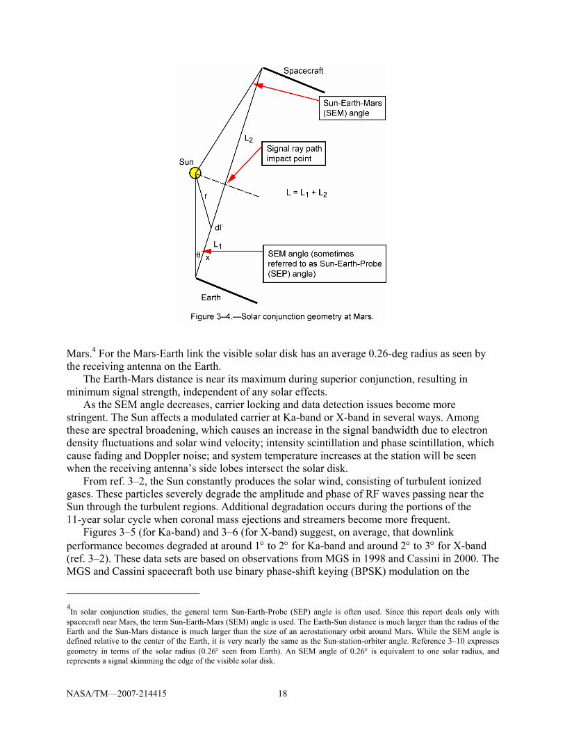
Radio signals passing near the Sun are affected by solar conjunction due to increased numbers of intervening charged particles causing intensity scintillation (fades) and phase scintillation of the spacecraft signals, leading to significant degradation. Signals on their way to or from a ground network site pass near the Sun in a superior conjunction (spacecraft, Sun, and Earth nearly in a straight line, with the spacecraft (near Mars in this case) on the opposite side of the Sun from the Earth).
Solar effects on communication are often expressed in terms of the Sun-Earth-Mars (SEM) angle. As shown in figure 3–4, the SEM angle is nearly the angular separation between the direction from the station to the center of the Sun and the direction to the spacecraft around
NASA/TM—2007-214415 18
Mars.4 For the Mars-Earth link the visible solar disk has an average 0.26-deg radius as seen by the receiving antenna on the Earth.
The Earth-Mars distance is near its maximum during superior conjunction, resulting in minimum signal strength, independent of any solar effects.
As the SEM angle decreases, carrier locking and data detection issues become more stringent. The Sun affects a modulated carrier at Ka-band or X-band in several ways. Among these are spectral broadening, which causes an increase in the signal bandwidth due to electron density fluctuations and solar wind velocity; intensity scintillation and phase scintillation, which cause fading and Doppler noise; and system temperature increases at the station will be seen when the receiving antenna’s side lobes intersect the solar disk.
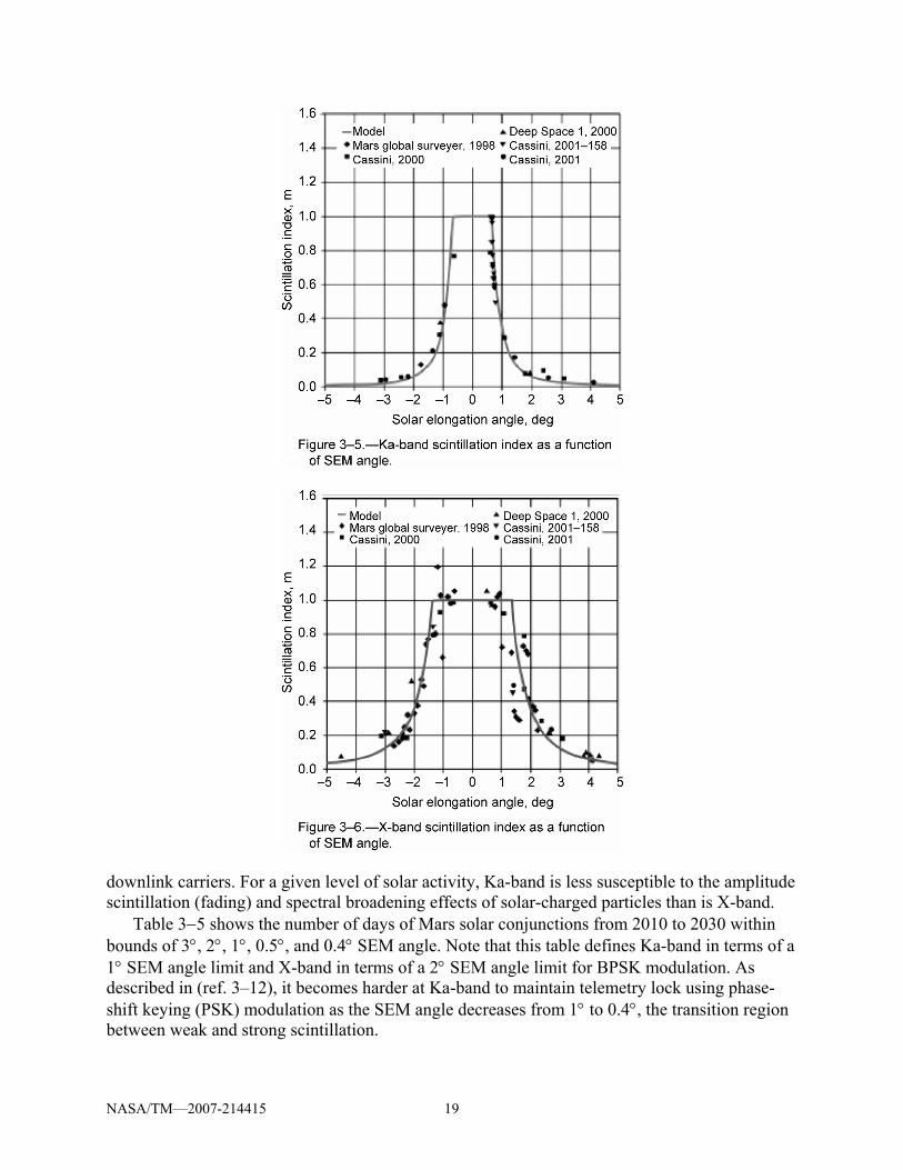
From ref. 3–2, the Sun constantly produces the solar wind, consisting of turbulent ionized gases. These particles severely degrade the amplitude and phase of RF waves passing near the Sun through the turbulent regions. Additional degradation occurs during the portions of the 11-year solar cycle when coronal mass ejections and streamers become more frequent.
Figures 3–5 (for Ka-band) and 3–6 (for X-band) suggest, on average, that downlink performance becomes degraded at around 1° to 2° for Ka-band and around 2° to 3° for X-band (ref. 3–2). These data sets are based on observations from MGS in 1998 and Cassini in 2000. The MGS and Cassini spacecraft both use binary phase-shift keying (BPSK) modulation on the
4In solar conjunction studies, the general term Sun-Earth-Probe (SEP) angle is often used. Since this report deals only with spacecraft near Mars, the term Sun-Earth-Mars (SEM) angle is used. The Earth-Sun distance is much larger than the radius of the Earth and the Sun-Mars distance is much larger than the size of an aerostationary orbit around Mars. While the SEM angle is defined relative to the center of the Earth, it is very nearly the same as the Sun-station-orbiter angle. Reference 3–10 expresses geometry in terms of the solar radius (0.26° seen from Earth). An SEM angle of 0.26° is equivalent to one solar radius, and represents a signal skimming the edge of the visible solar disk.
NASA/TM—2007-214415 19
downlink carriers. For a given level of solar activity, Ka-band is less susceptible to the amplitude scintillation (fading) and spectral broadening effects of solar-charged particles than is X-band.
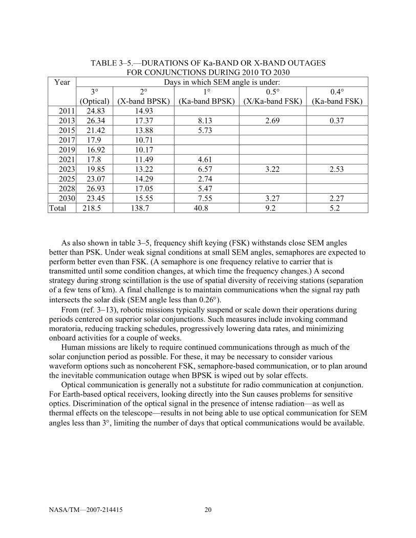
Table 3−5 shows the number of days of Mars solar conjunctions from 2010 to 2030 within bounds of 3°, 2°, 1°, 0.5°, and 0.4° SEM angle. Note that this table defines Ka-band in terms of a 1° SEM angle limit and X-band in terms of a 2° SEM angle limit for BPSK modulation. As described in (ref. 3–12), it becomes harder at Ka-band to maintain telemetry lock using phase-shift keying (PSK) modulation as the SEM angle decreases from 1° to 0.4°, the transition region between weak and strong scintillation.
NASA/TM—2007-214415 20
TABLE 3–5.—DURATIONS OF Ka-BAND OR X-BAND OUTAGES
FOR CONJUNCTIONS DURING 2010 TO 2030 Days in which SEM angle is under: Year
As also shown in table 3–5, frequency shift keying (FSK) withstands close SEM angles better than PSK. Under weak signal conditions at small SEM angles, semaphores are expected to perform better even than FSK. (A semaphore is one frequency relative to carrier that is transmitted until some condition changes, at which time the frequency changes.) A second strategy during strong scintillation is the use of spatial diversity of receiving stations (separation of a few tens of km). A final challenge is to maintain communications when the signal ray path intersects the solar disk (SEM angle less than 0.26°).
From (ref. 3−13), robotic missions typically suspend or scale down their operations during periods centered on superior solar conjunctions. Such measures include invoking command moratoria, reducing tracking schedules, progressively lowering data rates, and minimizing onboard activities for a couple of weeks.
Human missions are likely to require continued communications through as much of the solar conjunction period as possible. For these, it may be necessary to consider various waveform options such as noncoherent FSK, semaphore-based communication, or to plan around the inevitable communication outage when BPSK is wiped out by solar effects.
Optical communication is generally not a substitute for radio communication at conjunction. For Earth-based optical receivers, looking directly into the Sun causes problems for sensitive optics. Discrimination of the optical signal in the presence of intense radiation—as well as thermal effects on the telescope—results in not being able to use optical communication for SEM angles less than 3°, limiting the number of days that optical communications would be available.
NASA/TM—2007-214415 21
3.5 Spectrum (Ka-Band Frequency Allocations)
Mission Category Definitions Category A: Maximum spacecraft-Earth range less than 2 million km Category B (deep space): Maximum spacecraft-Earth range greater than 2 million km Thus, a lunar or Earth-Moon L2 mission5 is a Category A, and a Mars mission is a
Category B.
Spectrum Allocations Lunar and deep space missions, human and robotic, have different Ka-band frequency
allocations. Table 3–6 defines the uplink (forward) and downlink (return) link allocations, as recommended by the Space Frequency Coordination Group (SFCG).
TABLE 3–6.—Ka-BAND FREQUENCY ALLOCATIONS
Mission category
Mission Uplink (forward) band (GHz)
Downlink (return) band (GHz)
A TDRSS None 25.5 to 27.0 A Lunar, L2; human and robotic (SFCG) None 37.5 to 38.0 B Deep space robotic exploration 34.2 to 34.7 31.8 to 32.3 B Deep space human and robotic
exploration (SFCG)* 40.0 to 40.5 37.0 to 37.5
* Includes deep space technology demonstration in near-Earth regions.
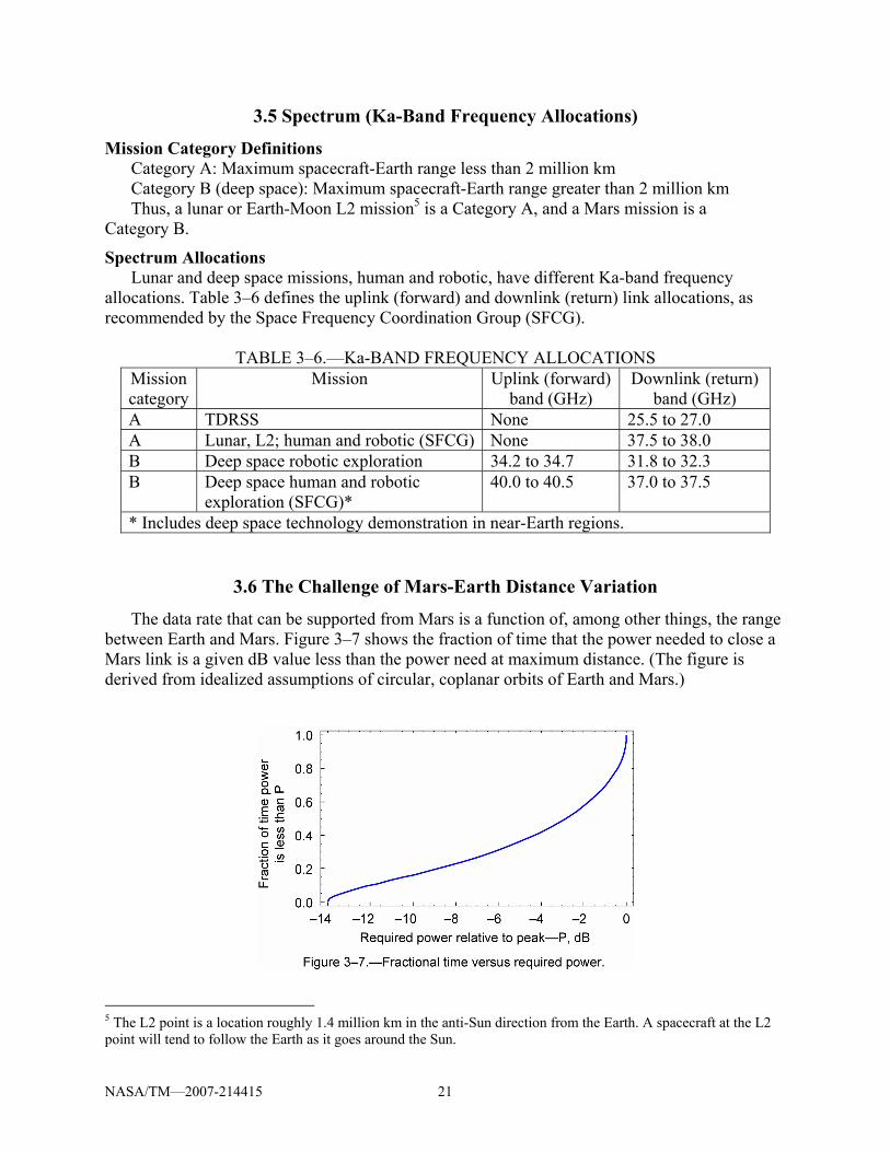
3.6 The Challenge of Mars-Earth Distance Variation
The data rate that can be supported from Mars is a function of, among other things, the range between Earth and Mars. Figure 3–7 shows the fraction of time that the power needed to close a Mars link is a given dB value less than the power need at maximum distance. (The figure is derived from idealized assumptions of circular, coplanar orbits of Earth and Mars.)
5 The L2 point is a location roughly 1.4 million km in the anti-Sun direction from the Earth. A spacecraft at the L2 point will tend to follow the Earth as it goes around the Sun.
NASA/TM—2007-214415 22
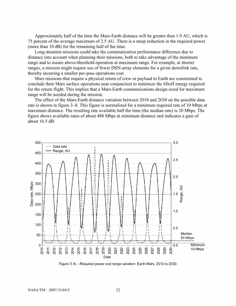
Approximately half of the time the Mars-Earth distance will be greater than 1.9 AU, which is
75 percent of the average maximum of 2.5 AU. There is a steep reduction in the required power (more than 10 dB) for the remaining half of the time.
Long-duration missions could take the communication performance difference due to distance into account when planning their missions, both to take advantage of the minimum range and to assure above-threshold operation at maximum range. For example, at shorter ranges, a mission might require use of fewer DSN-array elements for a given downlink rate, thereby incurring a smaller per-pass operations cost.
Mars missions that require a physical return of crew or payload to Earth are constrained to conclude their Mars surface operations near conjunction to minimize the liftoff energy required for the return flight. This implies that a Mars-Earth communications design sized for maximum range will be needed during the mission.
The effect of the Mars-Earth distance variation between 2010 and 2030 on the possible data rate is shown in figure 3–8. This figure is normalized for a minimum required rate of 10 Mbps at maximum distance. The resulting rate available half the time (the median rate) is 20 Mbps. The figure shows available rates of about 480 Mbps at minimum distance and indicates a gain of about 16.5 dB.
NASA/TM—2007-214415 23
3.7 References
3−1 Noreen, G., et al.: Mars Telecommunications Orbiter Ka-Band Operations., 9th Ka and Broadband Communications Conference, Lacco Ameno, Italy, Nov. 2003.
3−2 DSMS Telecommunications Link Design Handbook, TMOD No. 810−005, Rev. E, Jet Propulsion Laboratory, California Institute of Technology, Pasadena, CA, Jan. 2001. (This report contains information from module 101 (70-m subnet), module 103 (34-m HEF subnet), module 104 (34-m BWG subnet), module 105 (atmospheric effects), and module 106 (solar effects.)
3−3 Gatti, M.S.: The Deep Space Network Array. IEEE Microwaves and Theory and Techniques (MTT) Workshop on Arrays, June 17, 2005.
3−4 Statman, J., et al.: Deep Space Mission Systems (DSMS) Array Update, to JPL Executive Management Board, Jan. 18−19, 2005 (internal JPL document).
3−5 Gatti, M.S.: Private communication. Nov. 10, 2005. 3−6 Gatti, M.S.: The Deep Space Network Large Array. IPN Progress Report, vol. 42−157,
pp. 1−9, May 15, 2004. 3−7 Harcke, L.J., et al.: Recent Ka-Band Weather Statistics for Goldstone and Madrid. TDA
Progress Report, vol. 42−125, Jet Propulsion Laboratory, Pasadena, CA, May 1996. 3−8 Morabito, D.: Ka-Band Atmospheric Induced Temperature Fluctuations. IPN Progress
Report, vol. 42−150, Jet Propulsion Laboratory, Pasadena CA, Aug. 2002. 3−9 Shambayati, S.: On the Benefits of Short-Term Weather Forecasting for Ka-Band.
Aerospace, 2004. 3−10 Shambayati, S.: Maximization of Data Return at X-Band and Ka-Band on the DSN’s
34-Meter Beam-Waveguide Antennas. TMO Progress Report, vol. 42−148, Jet Propulsion Laboratory, California Institute of Technology, Pasadena, CA, Feb. 2002.
3−11 Davarian, F., et al.: Deep Space Ka-Band Link Management and Mars Reconnaissance Orbiter: Long Term Weather Statistics Versus Forecasting. IEEE Proceedings, vol. 92 1879−1894, Dec. 2004.
3−12 Morabito, D. and Hastrup, R.: Communicating With Mars During Periods of Solar Conjunction. IPN Progress Report, vol. 42−147, Jet Propulsion Laboratory, Pasadena CA, Nov. 2001.
3−13 Noreen, G., et al.: Integrated Network Architecture for Sustained Human and Robotic Exploration. 2005 IEEE Aerospace Conference, Big Sky, MT, Mar. 5, 2005, updated Dec. 28, 2004.
NASA/TM—2007-214415 25
Appendix 3A.—Calculation of Attenuation and System Noise Temperature
The following is from module 105 of (ref. 3−2). An attenuating atmosphere creates a noise temperature contribution to ground antenna system temperature. The atmospheric noise temperature at any elevation angle (θ) is calculated from the attenuation by
( ) ( ) KLTT patm ,11 ⎥⎦⎤
⎢⎣⎡ −= θθ
where Tp = mean physical temperature of atmosphere (K), calculated above
L(θ) = loss factor of atmosphere ⎥⎦⎤
⎢⎣⎡
= 10)(
10θA
A(θ) = atmospheric attenuation at any elevation angle (dB), calculated above
The following example will show a typical calculation of atmospheric noise temperature and
attenuation for a particular situation. The parameters for the example are (1) DSS 43, Canberra (2) Ka-band (32 GHz) (3) 90 percent year average weather (cumulative distribution, CD = 0.90) (4) 20° elevation angle (2.924 air masses) From table 3–1, the year average zenith attenuation is given as Azen = 0.41 dB. The attenuation at 20° elevation is
( ) ( ) dB181.120sin404.0%90,20 A ==°
The loss factor L at 20° elevation is ( ) 312.110%90,20 1181.0 ==° L The atmospheric mean physical temperature is Tp = 255 + 25×0.90 = 277.5 K The atmospheric noise temperature at 20° elevation is
( ) K991.65312.1115.277%90,20 Tatm =⎟
⎠⎞
⎜⎝⎛ −=°
NASA/TM—2007-214415 26
The operating system noise temperature at any elevation angle and for any weather condition
is given by
( ) ( ) ( ) K CD TTCD T atmvacopop ,,, , θθθ += where ( )θvacopT , = vacuum system temperature at elevation angle θ from the appropriate
antenna performance module (101, 102, 103, or 104).
The system temperature at zenith is 24.6 K (table 3–1, Canberra year-average, 90 percent weather), as compared with 66.0 K at 20° elevation.
NASA/TM—2007-214415 27
4. Telecom Design for 1 Gbps, 500 Mbps, and 100 Mbps The telecom system for Mars to Earth communication downlink is designed for three data
rate capabilities for a Mars relay. The three design points are 1 Gbps, 500 Mbps, and 100 Mbps at the maximum range of 2.67 AU, corresponding to the furthest point from Earth for the relay satellite. This communication link is designed for a Ka-band downlink with 90 percent link availability.
4.1 Design Approach
The design approach for the links uses the reference link budget shown in appendix 4A. In designing the three links there is a trade space that is three dimensional namely, ground G/T satellite RF power and size of the satellite antenna. The link budget will calculate required EIRP for the required downlink data rate based on the assumptions in chapter 3 within the given trade space. The satellite assumptions used in the link budgets include 90 percent link availability, BPSK/QPSK (quaternary phase-shift keying) modulation and LDPC (low-density parity-check) coding 1 dB satellite antenna pointing loss, 60 percent antenna efficiency, and 0.5 dB circuit losses. The 1 dB antenna pointing loss will dictate the antenna pointing accuracy, which is dependent on antenna size. The pointing accuracy requirement will determine whether a fine- pointing mechanism would be needed, for example, when the antenna size becomes large enough such that the pointing accuracy derived by the ACS is insufficient to keep the pointing loss within 1 dB.
The Earth assumptions include receiver G/T based on the DSN array of 12-m antennas. Three G/T assumptions are used for the trade space based on the ground network options of 180-, 45-, and 12-element arrays. The combining loss of the array is assumed to be 0.5 dB, and the radio implementation loss is assumed to be 1 dB. A 34-m antenna is not assumed in the link, but it is important to note that the G/T of a 34-m antenna is similar to DSN array of approximately ten 12-m antennas.
The maximum bandwidth available for Ka-band downlink is 500 MHz; dual polarization is assumed in the link analysis where applicable. Other possible options, such as BEM, are evaluated in the cases where high data rates may be feasible within the 500-MHz bandwidth constraint. The tables in appendix 4B show various modulation techniques and required Eb/No for appropriate bandwidth efficient modulation. (It is important to observe that the table does not exhaust the available options. For example, trellis-coded modulation could be used to moderate data rates to save 3 to 6 dB in Eb/N0.) The Eb/N0 in these tables is used to calculate link budgets when the links require bandwidth-efficient modulation.
For a given EIRP requirement, the spacecraft parameters can be optimized to minimize the RF mass of the spacecraft. It is shown in the following equation that the spacecraft communications subsystem mass (ma + p) can be minimized when the mass of the antenna (ma) is the same as the power mass (mp). Appendix 4C shows the derivation process of this mass minimization approach.
πηλ===+
apt
papapa L
ddmmm
EIRP22
NASA/TM—2007-214415 28
To minimize the mass of the spacecraft, the antenna system and power system masses will be equal. The antenna system mass comprises a reflector, a boom or a body mounting subsystem, portions of ADCS subsystem, and a fine-pointing subsystem. The antenna mass is estimated as a multiple of reflector area; the assumed density is 2 kg/m2, that is, the antenna mass is computed using the formula )kg/m 2()4/( 22 ⋅= Dma π .
The power system includes the amplifier and other elements that provide power such as an amplifying device, Electronic Power Converter (EPC), solar array, and radiator subsystem.
Table 4–1 provides a power summary and indicates mass density for the power system as a function of output power. The power mass is computed based on the required output power using the power density factor shown in the last column of the table. In cases where dual polarization assumption is used, additional amplifier mass is included in the total power mass.
TABLE 4–1.—MARS POWER SUMMARY Device Electronic power
convertor (EPC) Power
(watts) and device type
Eff., %
Mass, kg
Volume, cm3
Mass, kg
Volume, cm3
Solar array mass,
91 W/kg
Radiator mass,
67 W/kg
Total mass,
kg
Power density,kg/W
100 (Helical Ka-band TWT)
60 2.5 3000 1.5 2250 1.8 kg 1 kg 6.8 0.068
180 (Helical Ka-band TWT)
55 2.5 3000 1.5 2250 3.6 kg 2.2 kg 9.8 0.054
250 (Helical Ka-band TWT)
50 to 55
3.0 3500 2.5 3375 5.0 kg 3.1 kg 13.6 0.054
1000 (By combining four 250 W TWTs using magic-T hybrid.)
45 to 50
13 15500 10 13500 22 kg 15 kg 60 0.060
4.2 Link Design and Trade Study
The first step is to use the design scenario assumptions as stated in chapter 2. A reference Ka-band link budget is constructed based on this scenario and a downlink Ka-band link design is performed for 1 Gbps, 500 Mbps, and 100 Mbps using these link budgets. The link budgets are calculated for link between Mars and Earth using the assumptions stated in chapter 3 and in section 4.1. Link budget analysis determines the spacecraft parameters for each ground option
NASA/TM—2007-214415 29
and for each data rate design point at maximum Earth-Mars range, 2.67 AU. These parameter derivations also include the mass minimization approach indicated above. Further, when the range between Earth and Mars attains its minimum (0.38 AU), there is an increase in the link margin to about 14 to 17 dB that allows one to use that margin to trade among (1) increasing the downlink data rate; (2) reducing the number of antenna elements in the ground network; and (3) applying power conservation methods on the spacecraft.
A summary of results for three data rate design points (1 Gbps, 500 Mbps, and 100 Mbps) and three ground network options (180, 45, and 12 elements) are provided in tables 4–2, 4–3, and 4–4. The tables have a common structure. In table 4–2, for each ground network option, the spacecraft parameters for 1 Gbps at 2.67 AU are shown in the green highlighted rows in each table. Then the link is reevaluated for minimum range (cells highlighted in blue). Finally, the link is evaluated for BEM (cells highlighted in yellow). Tables 4–3 and 4–4 do the same for rates 500 and 100 Mbps, respectively. Each table provides a summary of the trade parameters and various options available for a given communication link, as discussed below.
Table 4–2 shows a summary of results for 1 Gbps for three different ground options. The results indicate that at 2.67 AU, a 4.5-m antenna and a 0.6-kW amplifier are required for a 180-element array ground network, whereas links with 45- and 12-element arrays require antennas and amplifiers of 6.2 m, 1.1 kW and 8.7 m, 2.2 kW, respectively.
TABLE 4–2.—SUMMARY OF RESULTS FOR 1 Gbps LINK (MARS TO EARTH)
Notes: a. 1-Gbps data rate assumes dual polarization with 500 Mbps for each polarization due to bandwidth constraint at Ka-band. b. Green highlight with blue font is reference point to determine spacecraft parameters for link design at max. range of 2.67 AU. c. Blue highlight indicates the trade between link capability and decrease in ground elements when range is reduced to 0.38 AU. d. Yellow highlight indicates the link designed with BEM. e. Fuchsia font indicates various options that can be chosen for minimum range of 0.38 AU between Earth and Mars;
a 34-m antenna is similar to an array with 10 elements. f. Results in the table include mass optimization.
There is an increase in spacecraft EIRP when the number of elements in the DSN array is
reduced, resulting in an associated increase in the spacecraft antenna size and power requirements and the consequent mass. We have already observed that given a spacecraft design,
DataRate(Mbps)
Range(AU)
SCAnt(m)
Ant Mass(kg)
SAntPtgEr(mdeg)
SCRFOut(kW)
Amp Mass(Kg)
SC-EIRP(dB)
Ground Network
GndGain(dB)
T_Gain(dB)
T_Mass(Kg)
Comments
Link Design 1Gbps at 2.67 AU with 180 element DSN-array (Dual polarization with each at 500Mbps)1000 2.67 4.5 31.80863 30 0.6 38.4 119.02 Array-180 92.95 211.97 70.208626 Dual Polarization (500Mbps)9000 0.38 4.5 31.80863 30 0.6 38.4 119.02 Array-180 92.95 211.97 70.208626 Link Capability only (single polarization)1000 0.38 4.5 31.80863 30 0.6 38.4 119.02 Array-4 76.42 195.44 70.208626 Dual Polarization (500Mbps)2000 0.38 4.5 31.80863 30 0.6 38.4 119.02 Array-180 92.95 211.97 70.208626 BEM - 8PSK Dual Polarization (1Gbps)2000 0.38 4.5 31.80863 30 0.6 38.4 119.02 Array-35 85.84 204.86 70.208626 BEM - 8PSK Dual Polarization (1Gbps)
Link Design 1Gbps at 2.67 AU with 45 element DSN-array (Dual polarization with each at 500Mbps)1000 2.67 6.2 60.38141 20 1.1 65.4 124.58 Array-45 86.93 211.51 125.78141 Dual Polarization (500Mbps)15000 0.38 6.2 60.38141 20 1.1 65.4 124.58 Array-45 86.93 211.51 125.78141 Link Capability only w/ single polarization1000 0.38 6.2 60.38141 20 1.1 65.4 124.58 Array-1 70.4 194.98 125.78141 Dual Polarization (500Mbps)2000 0.38 6.2 60.38141 20 1.1 65.4 124.58 Array-45 86.93 211.51 125.78141 BEM - 8PSK Dual Polarization (1Gbps)2000 0.38 6.2 60.38141 20 1.1 65.4 124.58 Array-8 79.43 204.01 125.78141 BEM - 8PSK Dual Polarization (1Gbps)
Link Design 1Gbps at 2.67 AU with 12 element DSN-array (Dual polarization with each at 500Mbps)1000 2.67 8.7 118.8936 14 2.2 124.8 130.56 Array-12 81.19 211.75 243.69357 Dual Polarization (500Mbps)20000 0.38 8.7 118.8936 14 2.2 124.8 130.56 Array-12 81.19 211.75 243.69357 Link Capability only (single polarization)2000 0.38 8.7 118.8936 14 2.2 124.8 130.56 Array-1 70.4 200.96 243.69357 Link Capability only (single polarization)2000 0.38 8.7 118.8936 14 2.2 124.8 130.56 Array-12 81.19 211.75 243.69357 BEM - 8PSK Dual Polarization (1Gbps)2000 0.38 8.7 118.8936 14 2.2 124.8 130.56 Array-2 73.41 203.97 243.69357 BEM - 8PSK Dual Polarization (1Gbps)
NASA/TM—2007-214415 30
decreasing the range between Earth and Mars to its minimum (0.38 AU) results in an increase in the link margin that can be used to trade between increasing the data rate and reducing the number of ground-array elements. As seen in the table, a 180-element ground array designed for 1 Gbps at 2.67 AU can support the same data rate at minimum range with just four of its elements. Or, with a 180-element array, the link could theoretically support 9 Gbps by scaling the modulation waveform. But due to the bandwidth constraint of 500 MHz, this scaling cannot work; a BEM is required.
With BEM chosen from the appendix D table, the link can support at most 2 Gbps, since the required Eb/N0 increases with BEM and the power requirement doubles in doubling the data rate. A more exhaustive modulation search might yield a further data rate increase. The results also indicate that regardless of the ground network configuration, a link designed for 1 Gbps at maximum range will not achieve a data rate increase of 14 dB at minimum range. Though the link has the power capability to support more than 2 Gbps, the combination of bandwidth constraints and the increased Eb/N0 required for BEM limits the achievable data rate to the 1 to 2 Gbps region.
Table 4–3 shows a comparable summary of results for a 500-Mbps maximum range design. As seen from the results, a 3.9-m antenna with a 0.45-kW amplifier is required to design for a 2.67 AU and a 180-element array. The spacecraft parameters change to 5.3 m, 0.8 kW and 7.4 m, 1.6 kW for 45- and 12-element arrays, respectively. As before, the impact of a reduction on array elements is an increase in the spacecraft EIRP and other parameters. The result for minimum range communications is consistent; support of data rates 500 MHz to 2 Gbps, again due to the bandwidth constraint and the BEM-induced increase in Eb/N0.
TABLE 4–3.—SUMMARY OF RESULTS FOR 500 Mbps LINK (MARS TO EARTH)
Notes: a. 1-Gbps data rate assumes dual polarization with 500 Mbps for each polarization due to bandwidth constraint at Ka-band. b. Green highlight with blue font is reference point to determine spacecraft parameters for link design at max. range of 2.67 AU. c. Blue highlight indicates the trade between link capability and decrease in ground elements when range is reduced to 0.38 AU. d. Yellow highlight indicates the link designed with BEM. e. Fuchsia font indicates various options that can be chosen for minimum range of 0.38 AU between Earth and Mars;
a 34-m antenna is similar to an array with 10 elements. f. Results in the table include mass optimization.
DataRate(Mbps)
Range(AU)
SCAnt(m)
Ant Mass(kg)
SAntPtgEr(mdeg)
SCRFOut(kW)
Amp Mass(Kg)
SC-EIRP(dB)
Ground Network
GndGain(dB)
T_Gain(dB)
T_Mass(Kg)
Comments
Link Design 500Mbps at 2.67 AU with 180 element DSN-array (Dual polarization with each at 250Mbps)500 2.67 3.9 23.89181 40 0.45 29.7 115.69 Array-180 92.95 208.64 53.591812 Dual Polarization (250Mbps)4000 0.38 3.9 23.89181 40 0.45 29.7 115.69 Array-180 92.95 208.64 53.591812 Link Capability only (single polarization)1000 0.38 3.9 23.89181 40 0.45 29.7 115.69 Array-8 79.43 195.12 53.591812 Dual Polarization (500Mbps)500 0.38 3.9 23.89181 40 0.45 29.7 115.69 Array-4 76.42 192.11 53.591812 Dual Polarization (250Mbps)2000 0.38 3.9 23.89181 40 0.45 29.7 115.69 Array-180 92.95 208.64 53.591812 BEM - 8PSK Dual Polarization (1Gbps)
Link Design 500Mbps at 2.67 AU with 45 element DSN-array (Dual polarization with each at 250Mbps)500 2.67 5.3 44.12367 25 0.8 48.6 121.72 Array-45 86.93 208.65 92.723669 Dual Polarization (250Mbps)8000 0.38 5.3 44.12367 25 0.8 48.6 121.72 Array-45 86.93 208.65 92.723669 Link Capability only (single polarization)1000 0.38 5.3 44.12367 25 0.8 48.6 121.72 Array-2 73.41 195.13 92.723669 Dual Polarization (500Mbps)500 0.38 5.3 44.12367 25 0.8 48.6 121.72 Array-1 70.4 192.12 92.723669 Dual Polarization (250Mbps)2000 0.38 5.3 44.12367 25 0.8 48.6 121.72 Array-45 86.93 208.65 92.723669 BEM - 8PSK Dual Polarization (1Gbps)2000 0.38 5.3 44.12367 25 0.8 48.6 121.72 Array-16 82.44 204.16 92.723669 BEM - 8PSK Dual Polarization (1Gbps)
Link Design 500Mbps at 2.67 AU with 12 element DSN-array (Dual polarization with each at 250Mbps)500 2.67 7.4 86.01681 18 1.6 91.8 127.62 Array-12 81.19 208.81 177.81681 Assume Dual polarization with11000 0.38 7.4 86.01681 18 1.6 91.8 127.62 Array-12 81.19 208.81 177.81681 Link Capability only (single polarization)1000 0.38 7.4 86.01681 18 1.6 91.8 127.62 Array-1 70.4 198.02 177.81681 Dual Polarization (250Mbps)2000 0.38 7.4 86.01681 18 1.6 91.8 127.62 Array-12 81.19 208.81 177.81681 BEM - 8PSK Dual Polarization (1Gbps)2000 0.38 7.4 86.01681 18 1.6 91.8 127.62 Array-4 76.42 204.04 177.81681 BEM - 8PSK Dual Polarization (1Gbps)
NASA/TM—2007-214415 31
Table 4–4 shows a summary of results for 100 Mbps for three different ground options for DSN array. The results for antenna size and power follow the pattern seen in the prior two tables. With regard to link capability at range 0.38 AU, the results remain consistent with previous one in that the link can support no more than 2 Gbps due to bandwidth and Eb/N0 constraints.
TABLE 4–4.—SUMMARY OF RESULTS FOR 100 Mbps
COMMUNICATION LINK MARS TO EARTH
Notes: a. 1-Gbps data rate assumes dual polarization with 500 Mbps for each polarization due to bandwidth constraint at Ka-band. b. Green highlight with blue font is reference point to determine spacecraft parameters for link design at max. range of 2.67 AU. c. Blue highlight indicates the trade between link capability and decrease in ground elements when range is reduced to 0.38 AU. d. Yellow highlight indicates the link designed with BEM. e. Fuchsia font indicates various options that can be chosen for minimum range of 0.38 AU between Earth and Mars;
a 34-m antenna is similar to an array with 10 elements. f. Results in the table include mass optimization.
Some key results in the tables can be displayed graphically. Figure 4–1 shows how antenna
size varies versus data rate, parametric in the ground array size. Figure 4–2 indicates an amplifier range from 0.25 to 2.2 kW over the same range of rates. Both figures pertain to a Mars-to-Earth communication link at 2.67 AU for three ground network array size options.
The next four figures explore the achievable data rate versus link margin (or distance), parametric in the data rate selected for maximum range. These calculations show the extent to which the spacecraft may allocate its additional link margin to more bandwidth-efficient modulation methods that increase the data rate. These results assume that (1) the exploration bandwidth allocated for the Mars satellite relay transmission to Earth is fixed at 500 MHz; (2) the EIRP has been designed for the maximum distance to Earth; and (3) all of this available EIRP is utilized to maximize the data rate when the range is less than the maximum. Of course, the link margin achieved by decreased range could be used in other advantageous ways; clearly reduced data rates occur if some of the EIRP margin is used to reduce either the Earth G/T and/or spacecraft (S/C) transmit power.
DataRate(Mbps)
Range(AU)
SCAnt(m)
Ant Mass(kg)
SAntPtgEr(mdeg)
SCRFOut(kW)
Amp Mass(Kg)
SC-EIRP(dB)
Ground Network
GndGain(dB)
T_Gain(dB)
T_Mass(Kg)
Comments
Link Design 100Mbps at 2.67 AU with 180 element DSN-array 100 2.67 3 14.13717 45 0.26 17.16 111.86 Array-180 92.95 204.81 31.297167 Single polarization transmit1800 0.38 3 14.13717 45 0.26 17.16 111.86 Array-180 92.95 204.81 31.297167 Link Capability only (single polarization)1000 0.38 3 14.13717 45 0.26 17.16 111.86 Array-23 88.53 200.39 31.297167 Dual Polarization (500Mbps)100 0.38 3 14.13717 45 0.26 17.16 111.86 Array-4 76.42 188.28 31.297167 Single polarization transmit1800 0.38 3 14.13717 45 0.26 17.16 111.86 Array-180 92.95 204.81 31.297167 BEM - 8PSK Dual Polarization (900Mbps)
Link Design 100Mbps at 2.67 AU with 45 element DSN-array 100 2.67 4.2 27.70885 30 0.5 30.12 117.75 Array-45 86.93 204.68 57.828847 Single polarization transmit3000 0.38 4.2 27.70885 30 0.5 30.12 117.75 Array-45 86.93 204.68 57.828847 Link Capability only (single polarization)1000 0.38 4.2 27.70885 30 0.5 30.12 117.75 Array-5 77.39 195.14 57.828847 Dual Polarization (500Mbps)100 0.38 4.2 27.70885 30 0.5 30.12 117.75 Array-1 70.4 188.15 57.828847 Single polarization transmit1800 0.38 4.2 27.70885 30 0.5 30.12 117.75 Array-45 86.93 204.68 57.828847 BEM - 8PSK Dual Polarization (900Mbps)
Link Design 100Mbps at 2.67 AU with 12 element DSN-array 100 2.67 5.9 54.67942 20 1 57.12 123.58 Array-12 81.19 204.77 111.79942 Single polarization transmit4500 0.38 5.9 54.67942 20 1 57.12 123.58 Array-12 81.19 204.77 111.79942 Link Capability only (single polarization)1000 0.38 5.9 54.67942 20 1 57.12 123.58 Array-1 70.4 193.98 111.79942 Dual Polarization (500Mbps)
A set of seven modulation types described parametrically in table 4–5 are considered in this exercise. In figures 4−3 through 4−5 we show the data rates that can be achieved by each modulation type, excluding those that did not turn out to yield the highest data rate at any margin value within the range considered. Thus, for example, figure 4–3, which corresponds to a design for 1 Gbps at maximum range, has only five curves; two of the modulations, 8-PSK rate 3/4 (#2) and uncoded QPSK (#6) are dropped because there exists a better alternative at every distance. Similarly, figures 4−4 and 4−5, for 500 and 100 Mbps rates at maximum distance, exhibit only four and three modulations, respectively.
NASA/TM—2007-214415 33
TABLE 4–5.—MODULATION TYPES SELECTED FOR COMPUTING MAXIMUM ACHIEVABLE DATA RATE VERSUS DISTANCE, OR EQUIVALENTLY, MARGIN
The data rate curves increase in proportion to the linear margin until they reach the point at
which their bandwidth fills the allocation; beyond this saturation data rate, additional margin yields no further rate increase.6
Figure 4–3 enables one to trace the data rate and modulation format evolution as increasing amounts of margin become available. When the design is for 1 Gbps at 2.67 AU, the S/C can transmit rate-1/2 encoded QPSK modulation, as long as dual polarization is used to achieve 500 Mbps per polarization. Since the modulation fills the 500-MHz spectrum, additional margin
6Nyquist bandwidth is taken as the criterion for determining the saturation data rate. For example, modulation #3,
8-PSK TCM, rate 2/3, transmits 2 information bits per symbol. Multiplying this by the available bandwidth 500 MHz yields a peak rate of 1 Gbps within the bandwidth. On the figures, the saturation rate is double this value due to the assumption of dual polarization usage.
NASA/TM—2007-214415 34
cannot be used to increase the data rate until there is sufficient signal strength to permit substitution of a more bandwidth-efficient modulation. As the margin increases above 1.5 dB, rate-3/4 encoded 8-PSK Trellis-coded modulation (TCM) may be substituted, first at the same data rate (1 Gbps) and then a rate increasing with margin. This modulation, also, eventually consumes all available bandwidth, negating any further data rate increase from it at higher margins. The other three modulations shown in the figure all come into play at other margin levels.
NASA/TM—2007-214415 35
Similar behaviors are shown for the two lower data rates. It may seem surprising that even by
designing for one of the lower rates at the 2.67 AU distance, the additional margin still supports substantial gains in data rate.
Figure 4–6 collects the information from the three prior figures by presenting the peak data rate envelope that is found using the modulation that proves most efficient at each value of margin. There are undoubtedly other modulation/coding schemes that would fill in some of the data rate plateaus. A 16-PSK, rate 3/4 TCM would achieve a 3-Gbps peak rate, but could get there at a value of margin lower than what is found for uncoded 8-PSK.
4.3 Observations Concerning the Link Design Trade Study
The trade study in section 4.2 considers Mars-Earth communication links of 1 Gbps, 500 Mbps, and 100 Mbps for three DSN-array ground options of 180, 45, and 12 elements. The following observations can be made:
1. EIRP requirement results increase as the numbers of ground elements are reduced. With
this increase in EIRP, there is an associated increase in antenna size, amplifier size, and the RF mass of the spacecraft.
2. BEM usage assists in increasing the data rate only to about 3 Gbps when the range is minimum, that is, 0.38 AU.
3. It is difficult to convert new-found link margin into a corresponding data rate increase in a bandwidth-constrained environment. The margin must be used to support the rate increase itself as well as the SNR inefficiency encountered in transitioning to a more bandwidth-efficient (hence, less power-efficient) method of modulation and coding.
NASA/TM—2007-214415 36
4. The ultimate data rate that may be achieved at the point of closest approach is a rather weak function of the initial rate designed for 2.67 AU distance. Our examples span a factor of 10 in maximum distance design rate, and yet the rates achieved when the full 17-dB margin is in effect, all saturate at or near 3 Gbps. However, the lower the design rate, the more slowly the 3-Gbps asymptote is approached.
5. For the Mars example, the 17-dB range of signal variation is not wide enough to allow the eventual introduction of any nonconstant envelope modulations such as quadrature amplitude modulation (QAM). The high Eb/N0 requirements of these highly bandwidth-efficient modulation methods preclude their use because the margin cannot support them. As an example, it takes 23-dB margin before rate-3/4 encoded 64 QAM can be used to drive the data rate to 4 Gbps. Trellis-coded PSK can achieve close to this with a constant-envelope waveform.
6. The ability to increase data rate as the spacecraft comes closer to Earth can be used to increase the average data return, or throughput, achieved on a mission, as long as a large fraction of the data is highly delay tolerant.
4.4 Conclusions Concerning the Link Design Trade Study
A high-rate Ka-band downlink is feasible between Earth and Mars at a maximum range of 2.67 AU. This is feasible for all the design points of 1 Gbps, 500 Mbps, and 100 Mbps.
From all the link analysis for the various options, it was determined that a spacecraft antenna, ranging in the size from 3 to 9 m would be needed for the Mars-Earth Ka-band downlink, with associated power requirements of 0.25 to 2.2 kW. Chapters 5 and 6 discuss more on the antenna and power technologies to determine their feasibility.
When a link is designed for any one of these data rates at maximum range, there is an increase in link capability with the varying Earth-Mars distance. This variation allows one to take advantage of the link margin observed by trading between various options such as an increase in data rate or reducing the number of ground elements. The increase in the data rate is constrained by bandwidth limitation of 500 MHz, thus requiring bandwidth-efficient modulation. The option for BEM was studied and it was determined that though the increase in the link margin is about 14 to 17 dB from maximum range to minimum range between Earth to Mars, this does not directly translate into similar data rate increase. The maximum achievable data rate at the minimum range is 3 Gbps. This increase to 3 Gbps is beneficial if the original link is designed for 100 Mbps at maximum range. But for the higher initial data rate designs it might be better to expend the margin by reducing the number of ground elements or reducing the spacecraft power consumption while keeping the data rate unchanged.
NASA/TM—2007-214415 37
Appendix 4A.—Approach Used for Link Calculations Determine coding and Eb/N0 to meet QoS requirement (required Eb/N0 includes code
imperfectness and implementation losses)
Calculate required Pt/No
Pt/No= 10 log (data rate) + Eb/N0
Calculate required EIRP for each channel class based on reference budget:
EIRP = Pt/No – Ls – La – Ge – Lc – Lgp – Lsp – Lpo – No + M, where
Ls = space loss = –295.9 dB at 2.67 AU
La = atmospheric attenuation = –1.18 dB (90 percent weather)
Ge = gain of Earth antennas = number of antennas × gain of each
Lc = combining loss = –0.6 dB
Lgp = ground antenna pointing loss = –0.07 dB
Lsp = spacecraft antenna pointing loss = –1.0 dB
Lpol = polarization loss = –0.2 dB
No = noise spectral density (103.6° Top for 90 percent weather)
M = margin, 3 dB
NASA/TM—2007-214415 38
TABLE 4A–1.—KA-BAND REFERENCE LINK BUDGET
2.67 AU Range 37.25 GHz FrequencyLink Parameter Unit Design Fav Adv Mean Var. 20 deg ElevationTRANSMITTER PARAMETERS Value Tol Tol ValueTotal Transmitter Power dBm 56.53 0.45 kWCircuit losses dB -0.50S/C Antenna Gain dB 64.57 5.6 0.6 Diam, effAntenna Pointing Loss dB -1.01 0.025 Pointing Error (deg)
0.953147876 Pntg Error TermEIRP dBm 119.59
PATH PARAMETERSSpace Loss dB -295.90Atmospheric Attenuation dB -1.18
RECEIVER PARAMETERS Diameter Eff NEarth Station Antenna Gain dB 92.95 12 0.5 180 77.85388Receiver Circuit Loss dB -0.60 (combining loss)Pointing Loss dB -0.18 0.005 Pointing Error (deg)Polarization Loss dB -0.20 0.408491959 Pntg Error Term
TOTAL POWER SUMMARYTotal Received Power dBm -85.52Noise Spectral Density dBm/Hz -178.45 Top(K) 103.58 KPt/No dB-Hz 92.93 Hotbo 3.91 K
DATA CHANNEL PERFORMANCE Received Pt/No dB-Hz 92.93Telemetry Data Suppression dB 0.00Range Suppression dB 0.00Pd/No dB-Hz 92.93Data Rate dB-Hz -86.99 500000000 bpsAvailable Eb/No dB 5.94Radio Loss dB -1.00 All implementation losses combinedSubcarrier Demod Loss dB 0.00Symbol Sync Loss dB 0.00Waveform Distortion dB 0.00Output Eb/No dB 4.94Required Eb/No dB 1.00 LDPCPerformance Margin dB 3.94
NASA/TM—2007-214415 39
Appendix 4B.—Some Options for Bandwidth-Efficient Modulation
Figure 4–7.—Bandwidth-efficient modulation options for bandwidths of 500 MHz and 1 GHz.
Appendix 4C.—Derivation of Mass Optimization, Given a Required EIRP Much of the user burden analysis being used in assessing both RF and optical
communications payloads stems from the result due to G. Noreen in which the summed mass of the antenna and transmit power subsystems is minimized subject to a constant EIRP constraint (ref. 4C–1). In that formulation antenna mass is modeled as proportional to aperture squared, power mass proportional to transmit power.
In both subsystems there are components whose mass variations are practically decoupled from aperture size and output power; these could be included in the Noreen model as additive constants. As it turns out, these “zero-aperture” and “zero-power” constants (denoted as )0(
Am
and )o(
Pm below) do not affect the optimization process; one can optimize as though they were absent and add them in subsequently. The analysis below demonstrates this claim.
The antenna and mass models are thus 2)o( )4/( dKmM AAA π+= (4C.1) PKmM PPP += )o( (4C.2)
We minimize MT = MA + MP subject to a constant EIRP constraint. EIRP is expressed as
P
PP
A
AA
KmM
KmM
PdPdPG)()(4EIRP
)o()o(
22
22 −⋅
−⋅=⋅⎟
⎠⎞
⎜⎝⎛=⋅⎟
⎠⎞
⎜⎝⎛=⋅=
λπη
λπη
λπη (4C.3)
where the final expression above results from solving equations (4C.1) and (4C.2) for d2 and P, respectively. If we note that ATP MMM −= (4C.4) we can rewrite the EIRP as a function of MT and solve for MT:
P
PAT
A
AA
KmMM
KmM )()(4EIRP
)o()o(
2
−−⋅
−⋅=
λπη (4C.5)
Minimizing MT with respect to MA is found by setting
0)(
EIRP4
12)o(
2=
−⋅−=
∂∂
AA
PA
A
T
mM
KKMM
πηλ (4C.6)
leading to
ηλπ
πEIRP)4/(1ˆ
2)o( PA
AAKK
mM⋅
+= (4C.7)
NASA/TM—2007-214415 42
where the optimum mass (excluding the zero-aperture contribution) is denoted by
ηλπ
πμ
EIRP)4/(1 2PA KK ⋅
= (4C.8)
Substituting equations (4C.3) and (4C.4) into the total mass expression solved for PM yields
)o(2
)o(ˆEIRP
)ˆ(ˆˆ
PAAA
PAATP mM
mMKKMMM ++⎟
⎠⎞
⎜⎝⎛
−−=
πλ
η (4C.9)
(o)2
(o)ˆEIRP
4)ˆ(ˆˆ
PAAA
PAATP mM
mMKK
MMM ++−
−=πηλ (4C.10)
or
μηλπ
π+=
⋅+= )o(
2)o( EIRP)4/(1ˆ
PPA
PP mKK
mM (4C.11)
The optimum total mass is
μ
ηλπ
π2EIRP)4/(2
ˆˆˆ
)()(2
)()( ++=⋅
++=
+=
oP
oA
PAoP
oA
PAT
mmKKmm
MMM
(4C.12)
From equation (4C.12) one can find the optimum antenna size and power.
The optimum mass has the interesting interpretation that it is a scalar times the geometric mean of two masses, one representing the mass (Mλ) of a (fictitious) 1-λ antenna, 2)4/( λπλ AKM = , (4C.13) the other the mass of a power subsystem that generates the entire EIRP as watts, as though a 0-dB gain antenna were to be used: EIRPEIRP ⋅= PKM (4C.14)
4C.1 Reference
4C–1. Noreen, G., et al.: “Mars Exploration Deep Space Return Link Scenario and Transmit System Optimization,” IAC–05–B3.6.04, 2005.
NASA/TM—2007-214415 43
5. Enabling Technologies for Earth-Mars Communications: Part I, Antenna System
This chapter and the next present the technical challenges and enabling technologies for realization of a high-capacity Gbps-class RF communications system at technology readiness level (TRL) 6 by the year 2020. The overall goal for these technologies is to achieve the required EIRP with a system of sufficiently low mass that can be stowed for launch and transport to Mars. This involves a tradeoff between transmit power and antenna gain. A smaller antenna will reduce mass, simplify stowage, and minimize beam-pointing accuracy requirements. However, smaller antennas require much higher transmit power, which in turn places greater demand on the prime DC power generation system (solar cells and batteries). Since large-aperture antenna technology can substantially reduce the demand for RF power, developing a simple and practical antenna design has potential to provide high reliability and minimize overall system mass at an acceptable mission cost.
Referring back to the tables in section 4.2 will confirm that the requirements of communication scenarios for Mars can be met with antennas 6 to 25 m in size and power systems capable of delivering hundreds of watts to the antenna at Ka-band. This chapter addresses enabling technologies for a HGA system. Chapter 6 then discusses the technical challenges associated with generating high-RF transmit power. In these two chapters, we present a brief overview of the current state of the art for each technology, discuss current research directions, and finally indicate the key areas where research and development is needed to enable high-capacity RF communications.
As discussed in chapter 4, the goal is to minimize the RF subsystem mass in obtaining a desired EIRP. This includes the power system, the antenna itself, and any other spacecraft systems whose mass varies with the antenna aperture. Figure 5–1 describes the elements of two basic antenna configurations: a steerable antenna system and a body-mounted antenna system. The mass and complexity are lower in a body-mounted configuration for HGAs; thus the focus of this report is on the body-mounted antenna. It comprises a reflector, a fixture that attaches it to the spacecraft body, and an optional fine-pointing subsystem. The total mass is also impacted by the stowage and associated deployment mechanism utilized and the ADCS, whose masses may have to be increased to support the antenna system.
NASA/TM—2007-214415 44
Section 5.1 includes a review of the range of technology options considered, as
circumscribed by considerations such as the required data rate, spectral allocations, and understood limitations on technology. Also provided is an overview of some of the spacecraft layout and design issues associated with the inclusion of a large deployable reflector. The section on requirements concludes with a pair of detailed technical analyses regarding the limitations of antenna pointing using the spacecraft ADCS system. The first analysis provides an upper bound on antenna size for a system that employs spacecraft-only pointing that is based on the attitude holding capability of the spacecraft. Requirements on attitude holding are further analyzed based on the ability of a closed-loop pointing system (i.e., “autotrack”) to articulate the beam. The second analysis shows that a large reflector can be accommodated on a relay spacecraft without driving the size of the ADCS actuators to unreasonable levels.
Section 5.2 describes a number of options for the antenna system. Broad categories of options considered include reflectors, reflect arrays, and phased-array antennas. A detailed assessment of reflector-based options that include fine-beam pointing feeds is then presented.
Section 5.3 provides a detailed evaluation of the various options available for deployable reflector technology. The underlying technologies are described in some detail and the history of development of these technologies are reviewed. The final section of this chapter provides a qualitative assessment of the various technology options.
5.1 Antenna Requirements and the Antenna-ADCS Relationship
5.1.1 Achieving 1 Gbps at Distance of 2.67 AU
The primary antenna requirements considered for this report are derived from system flow down to support a nominal 1-Gbps data rate. The values summarized in table 5–1 cover the range of aperture size and RF power for the trade space considered in preceding chapters. Additionally, the nominal requirements given in the “comments” column of table 5–1 are consistent with the “minimum complexity” system that employs a ground-based receiver with a G/T equivalent to the coherent combination of forty-five 12-m satellite dishes, as discussed in chapter 7. The objective here is to assess the corresponding technical challenges. In this chapter we consider low-mass deployable antenna technologies in the range from 6 to 25 m.
In future MARS exploration missions, dual-band operations (X-band and Ka-band) may be utilized with the X-band handling the essential data and Ka-band the high data rates associated with science, robotic operations, and HDTV. This report only addresses dual-band antennas with respect to inflatable antennas (section 5.3.1.1).
NASA/TM—2007-214415 45
TABLE 5–1. NOMINAL REQUIREMENTS FOR A HIGH-CAPACITY TELECOM SYSTEM
Requirements Values Comments Tx freq. 37.5 to 38 GHz (Ka-band) Mars exploration band Tx bandwidth 500 MHz ~1.33% of center frequency Peak gain 65 to 77 dB 68 dB gain 9 m reflector nominal Tx RF power 0.82 to 2.89 kW 1 kW nominal, power-combined
TWTA or klystron Aperture efficiency ≥50% Low efficiency chosen to allow
Pointing loss 1 dB Large pointing loss assumed in fine-pointing analysis
Polarization Dual (right- and left-hand circular polarized)
Mass density goal 1 kg/m2 Complete antenna system-reflector plus deployment mechanism
Lifetime 10 years Environment MRO or MTO
In table 5–1 pointing loss is not relegated exclusively to the deep space antenna as a
requirement, but rather reflects the net performance of the system when imperfect pointing tolerances are included. For a smaller antenna (6 m diam.) the wide beamwidth obviously eases pointing requirements. In this case, the spacecraft attitude control system is believed to be sufficient to point the antenna so that the only pointing requirements relate to the knowledge and/or invariance of electrical boresight on orbit (e.g., following deployment, under thermal gradients, etc.). Conversely, for large antennas (>12 m diam.) it is likely that the system will require an active fine pointing control system. Requirements for such a system are described in the section 5.1.3 and implementation methods are considered in section 5.3.3.
5.1.2 Spacecraft Accommodation
The key S/C accommodation issue for high-capacity RF communications is stowage of a 6- to 25-m-class antenna. Launch vehicle shroud packing and transport to Mars (e.g., on the CEV) impose a stowage requirement that can only be achieved with a deployable antenna system. Stowed volume and package dimensions are important metrics that depend upon the deployment mechanism used to fold the antenna (see sec. 5.3.1). Other important characteristics of the deployment mechanism are complexity, reliability, and mass (see sec. 5.3.2).
Less obvious is the impact of the deployment mechanism on antenna optics design and spacecraft dynamics. For example, some of these deployment systems inherently favor a center-fed reflector, while others are more naturally suited to an offset-fed configuration. The choice of center-fed versus offset design can significantly alter system design due to the location of the feed relative to the transmitter. For a high-power system, waveguide losses and the resultant
NASA/TM—2007-214415 46
impact on RF gain and heat dissipation can impose important design constraints. In addition, the location of the feed point can alter the spacecraft moment of inertia, thereby imposing a limitation on the ability to point the antenna. This issue is taken up in the next section, but a point design exercise is needed to sort through the S/C accommodation tradeoffs and issues.
5.1.3 Fine-Beam-Pointing Requirements
A limitation presented by the spacecraft bus that affects the antenna aperture and amplifier power trade is the limited accuracy with which the transmitting and receiving antennas can be pointed at one another. Errors in transmitter and receiver antenna pointing lead to losses in the overall link SNR. For transmit and receiver antennas, the antenna pointing errors are required to be a small fraction of their antenna beamwidth in order to limit the composite losses.
On the spacecraft side, integrating a fine-pointing system into the communications and antenna system can mitigate pointing losses. This system points the transmit beam in the direction of the DSN receiver stations on Earth by directing the beam towards a “beacon” signal generated on or near the receiving antenna. This beacon signal can be a pure carrier tone or, alternatively, the forward communications link signal may serve as the tracking beacon. Such a receiving system is variously termed a “closed-loop tracking” system, an “autotrack,” or a “monopulse feed” system. It is the overall composite pointing error in relation to the antenna beamwidth then that dictates when fine-beam pointing is required. By placing a limit on pointing loss, as described below, this division is defined.
As the electrical size of a reflector antenna is increased, the beamwidth decreases. If the beamwidth is large in relation to the overall pointing error associated with a particular spacecraft, then antenna pointing can be accomplished solely through commanding the spacecraft’s attitude determination and control system. However, if the spacecraft is limited in its ability to hold a particular attitude, then a fine-beam-pointing system must be integrated within the antenna subsystem and closed-loop tracking of a transmitted RF signal, emanating from the receiver location must be employed. The crossover point between spacecraft pointing and closed-loop or fine-beam pointing is set by limiting pointing loss in the overall link equation.
Pointing loss, in dB, is related to the overall pointing accuracy, due to all sources including thermal beam wander, e and antenna beamwidth θ by
2
12 ⎟⎠⎞
⎜⎝⎛θ
=eLpoint
Thus, if the pointing loss is limited to be no more than a particular value, then the minimum
allowable beamwidth can be related to spacecraft-pointing accuracy. For a limit of 1 dB pointing loss the antenna beamwidth must be
e12>θ
If this condition is not met, then closed-loop, fine-beam pointing must be employed in order
to keep the antenna beam pointed at the receiver. Equivalently, a relationship between antenna aperture extent, D, and spacecraft pointing error can be derived through the direct relationship between aperture extent and beamwidth for aperture antennas:
NASA/TM—2007-214415 47
efc
D12
⎟⎠⎞
⎜⎝⎛ρ
<
Where ρ is the taper factor, c is the speed of light and f is the frequency. Using a 3σ value for
spacecraft holding threshold (one dimension) and assuming Gaussian deviates, the 1 dB pointing loss will be exceeded about 0.54 percent of the time or a little less than 8 minutes in 24 hours of operation. Taking the pointing error to be the 3σ spacecraft holding capability, the taper factor to be 1.27 (which corresponds to parabolic illumination) and a 38 GHz frequency of operation, the relationship between spacecraft antenna aperture and 3σ spacecraft pointing accuracy is shown in figure 5–2. The region above the curve is the area where closed-loop, fine-pointing systems are required. Below the curve antenna pointing may be achieved using the spacecraft ADCS alone.
Typical values for one-axis spacecraft attitude holding capability are given in table 5–2. Spacecraft holding values for current and projected spacecraft are in the range of 0.05 to 1.5 mrad. Note that existing spacecraft such as Cassini are capable of 0.1 mrad using reaction wheels. If a projection on the spread of 3σ spacecraft attitude holding capability for future spacecraft is taken to be between 0.15 and 0.35 mrads, then the associated spread on maximum antenna size is between about 8 and 19 meters. This mapping of the range of values of spacecraft holding capabilities and associated antenna diameters is shown in figure 5–2.
TABLE 5–2.—TYPICAL SPACECRAFT POINTING ACCURACIES
Reflector diameter,
m
Pointing accuracy (3 sigma, mrad)
MRO 3.0 1.5 MTO (estimate) 3.0 0.35 to 0.55 CASSINI 4.0 0.10 (react. wheel)
2.0 (thruster) GOES–N N/A 0.05 Aqua R 1.6 0.12
In order for a fine-beam-pointing system to work, the spacecraft must be able to control the transmit antenna pointing direction with accuracy sufficient to enable the system to search for and acquire a beacon signal. Once the Earth beacon is acquired, the fine-pointing system will manipulate the transmit beam so that it points back in the direction of the beacon signal and thereby drives the composite pointing error to a sufficiently low level that the pointing loss requirement is met. Acquisition of the beacon signal occurs during an “initialization” phase of operation in which the spacecraft receiver blindly searches over a range of angles for the beacon signal.
NASA/TM—2007-214415 48
Manipulation of the transmit beam is limited to a small range of angles that are described in
terms of their deviation from the antenna boresight. This limit is dictated by the shape of the reflector and, in general, increases with the ratio of the antenna focal length F to antenna diameter D or “F/D ratio” as well as the chosen feed technology. In this report, the limitation of the antenna, together with its fine-pointing system to capture a beacon signal is labeled the Fine Pointing Capture Ratio (FPCR) and is an expression of the number of nominal antenna beamwidths that the antenna can be scanned from boresight with its fine-pointing mechanism. The FPCR, together with other antenna parameters, can be used to determine spacecraft attitude holding requirements. Such requirements are provided in table 5–3. The spacecraft attitude holding requirements in table 5–3 are provided for antennas of several diameters for 37.5 GHz and a variety of FPCR values. These values are derived to achieve a pointing loss less than 1 dB and are given for FPCR values of 0, 3, and 7. The value FPCR = 0 corresponds to the case in which the antenna is pointed solely with the spacecraft ADCS, which results in stringent pointing requirements. Note that the larger FPCR values correspond to less stringent attitude holding requirements on the spacecraft. The FPCR that can be achieved depends upon the technical approach used to implement the beam steering. Section 5.2.2 presents antenna system concepts that are capable of performing active fine-beam-pointing control. Specific technical details on implementation of fine-beam-pointing systems are addressed in section 5.3.3.
NASA/TM—2007-214415 49
TABLE 5–3.—SPACECRAFT POINTING REQUIREMENTS AS A FUNCTION OF FPCR AND ANTENNA
Point requirement (mrad)L point = 1 dB, FPCR = … (BW )
5.1.4 ADCS Sizing
For large deployable antennas the potential exists for integration of the antenna into the spacecraft to dominate the sizing of the required attitude control system. The structure of the large reflector adds to the spacecraft moment of inertia and increases the magnitude of the disturbance torques; the larger the antenna, the more pronounced are these effects. Furthermore, the antenna beamwidth is inversely proportional to the antenna extent and thus the pointing requirements are made more challenging by the use of larger antennas. An abbreviated analysis of the effects of antenna size on spacecraft ADCS is described here. The analysis consists of estimating the size of the ADCS actuators of a spacecraft that employs large antennas using design equations and methods from (ref. 5–1). The general flow of the prescribed analysis is to determine the magnitude of the disturbance torques for the spacecraft and then to use simplified equations for sizing reaction wheels and momentum wheels for the attitude control system.
The analysis assumes a nominal spacecraft of 800 kg with dimensions of 1 by 2 by 3 m. Additionally, an underlying assumption of the analysis is that the antenna is mounted to the spacecraft in a body-fixed fashion with overall extents ranging from 6 to 25 m and areal densities (ρ) ranging from 1 to 2 kg/m2. The graph in figure 5–3 shows the effect of the integration of a large deployable antenna on spacecraft moment. Note that the spacecraft moment is not significantly affected by the antenna until the radius exceeds approximately 7.5 m (i.e., the extent is 15 m.) This appears to be true for the entire range of assumed areal densities for the antenna.
The analysis assumes a 1-m moment between spacecraft center of gravity and the center of solar pressure and a 1-m moment between the spacecraft center of mass and the center of aerodynamic pressure, corresponding to the case in which the center of the reflector is close to the body of the spacecraft. This design detail is included in order to reduce the magnitude of the disturbance torques due to solar pressure and aerodynamics to modest levels; the antenna would likely require a centrally fed reflector. It is further assumed in this analysis that the reflector technology provides a solid surface that does not transmit light or gas effectively. Disturbance torques from the atmosphere and the Sun would be less with a mesh technology or other technology that is less susceptible to solar pressures or atmospheric affects such as an inflatable reflector that is transparent and that employs a sheer coat of metallization or a composite technology that has openings. Note that the use of such technologies could provide for a reduction in the reaction wheel sizing.
NASA/TM—2007-214415 50
Note that disturbance torques are dominated by aerodynamic pressures for low altitudes. The
estimated torques are shown in figure 5–4 as a function of antenna radius for spacecraft altitudes of 207, 500, and 4000 km. Disturbance torques are a much stronger function of altitude than of antenna diameter. This is especially true for the lowest orbital altitude (207 km).
An estimate of reaction wheel mass was made by assuming that slewing rates are negligible for the nearly inertially pointed spacecraft. This estimate is based on scaling an Ithaco reaction wheel model TW–50E300, a large reaction wheel. This model of reaction wheel has a speed range of ±3850 rpm, wheel diameter of 39.3 cm, and maximum wheel mass of 10.6 kg.
Mass estimates for the size of the reaction wheels are provided in figure 5–5 for a number of different antenna sizes and spacecraft altitudes. For a spacecraft altitude of 4000 km, estimates of wheel size are provided for various antenna mass densities. Note that for a spacecraft altitude of 207 km the required reaction wheel exceeds the manufacturer’s specifications for all antenna sizes. This is due to the high level of disturbance torques placed on the spacecraft at the lower altitudes. The calculations also reveal that at 4000 km altitude the reaction wheel sizing is not a strong function of antenna areal density. For both the 500 and 4000 km altitudes the manufacturer’s specification of 10.6 kg for the reaction wheel size is exceeded for antennas greater than approximately 15 m in extent (7.5 m radius).
NASA/TM—2007-214415 51
In conclusion, since a Mars relay satellite will probably be placed at 4000 km or higher, the mass impact on the ADCS generated by antennas less than 15 m will not be significant. Furthermore, controlling the attitude of a spacecraft equipped with an antenna larger than 15 m may require the development of very large reaction wheels. Note that the conclusions of this analysis are directly applicable only to the above-described point design. Thusly, these
NASA/TM—2007-214415 52
conclusions cannot be valid for the more general cases considered in this report. A more comprehensive analysis would, necessarily, include determination of the sensitivity of the size of the actuation system to the parameters mentioned above, such as the size of the moment between the spacecraft center of mass and the center of aerodynamic pressure, etc. This analysis does, however, indicate that a large reflector on a relay spacecraft can be successfully accommodated without driving the size of the attitude control system actuators to unreasonable levels.
5.2 Large-Aperture Antenna Technologies and Architectures
5.2.1 Overview of Current Antenna State of the Art and Future Research Directions
There are several technologies that can be used to realize a 6- to 25-m-class deployable antenna. Technologies capable of providing the needed aperture area include reflector antennas, phased arrays, reflectarrays, and discrete element lenses. The principle of operation for the first three is illustrated in figure 5–6. As explained below, mesh reflector antennas are currently the predominant technology used in commercial and military telecommunications applications, but deployable reflectors with good stowage characteristics have not yet demonstrated high efficiency at Ka-band. The discussion below summarizes the current state of the art and suggests potential for each technology to achieve a low mass, low cost, TRL 6 antenna technology that supports Ka-band no later than the 2020 timeframe. Several 12-m-class antenna technologies are poised to achieve TRL 6 before 2010.
NASA/TM—2007-214415 53
5.2.1.1 Reflector Antennas Reflector antennas are currently the most widely deployed high-gain communications
antennas in space. Flight-proven methods to produce a doubly curved reflector (e.g., parabolic reflector) include solid surface composite reflectors and deployable reflectors. Deployable reflector technology includes mesh reflectors, inflatable reflectors and folded composites. The various types of reflectors are described in greater detail in section 5.3.1.
Deployable mesh reflectors are widely used for commercial telecommunications applications in Earth orbit due to their low mass density (typically 1 to 2 kg/m2 with deployment booms) and compact stowed volume (refs. 5–2 and 5–3). Because of launch vehicle shroud size limitations, deployable antennas are essential for apertures exceeding approximately 4.5 m. The key limitations of mesh reflectors at Ka-band are mesh reflectivity and surface accuracy. Commercial telecom applications typically use L-band and S-band, where surface accuracy and reflectivity demands are not challenged. The current state of the art is roughly Ku-band, and there are indications that a limit exists at about Ka-band above which mesh reflectors may not be practical. The stowed size of mesh reflectors is limited by folding the support structure. Deployment reliability is good, with about 40 modern mesh designs successfully deployed and operated in orbit. Apertures of 12 m have achieved TRL 9 in the commercial world. However there have been failures to deploy for mesh reflectors, such as on the Galileo mission.
Solid (nondeployable) composite reflectors have relatively low mass density (~3 to 4 kg/m2), very high surface accuracy, excellent reflectivity, and high efficiency. Although the size of a solid composite reflector is limited by the launch vehicle fairing diameter, the construction technique is of interest because it is used in solid element deployable antennas (discussed below) and deployment structures. In the typical composite structure, graphite epoxy face sheets are bonded to a nomex or aluminum honeycomb core. When high reflectivity is needed, the composite structure is coated with a metallic reflecting surface such as vapor-deposited aluminum (VDA). The inherent rugged construction and low coefficient of thermal expansion makes these reflectors ideal for harsh space environments. Flight units up to 4 m diameter at Ka-band have achieved TRL 9.
Solid element deployable antennas extend the size of composite reflectors by folding multiple composite surfaces. Such antennas are an excellent design solution for spaceborne applications that require larger aperture sizes operating at frequencies above approximately 30 GHz. The deployable aspect of this design allows for apertures exceeding 4.5 m, and the solid element aspect—with its greater surface precision—allows for RF operations at frequencies well above 30 GHz, the approximate performance limit for meshes. The solid elements themselves are usually lightweight composite structures (e.g., graphite-epoxy skins with aluminum-honeycomb core). The element shape can vary, ranging from simple folding edges (as in the ETS–VI antenna) to more complex, nested polygonal shapes (as in the TRW Sunflower).
Various folding techniques have been demonstrated in laboratory experiments and show promise for obtaining the reflectivity and surface accuracy needed for very high frequency reflectors. Solid element deployable reflectors have been demonstrated at frequencies as high as 94 GHz. It is likely this technology can achieve TRL 6 at Ka-band with good efficiency. However, the composite molding process is usually expensive, and the addition of a relatively complex mechanism to deploy the folded surfaces accurately into position means this is likely to be a comparatively high-cost option.
Inflatable structure technologies present a potentially very attractive design solution for large deployable antennas. Existing inflatable technology is considered capable of providing large
NASA/TM—2007-214415 54
apertures operating in the low- to mid-frequency regime, and several design concepts show promise for Ka-band. The Echo balloon—one of the earliest satellites of the space age—was an inflatable antenna structure, and interest in this class of structures has increased since the in-space demonstration of the Inflatable Antenna Experiment (IAE) in 1996. Inflatable structures are important because of their potential to enable a new class of lightweight large-aperture structures requiring very high packaging efficiency. Additionally, many inflatable concepts allow insertion of the stowed package in irregularly shaped spaces. Furthermore, inflatable solutions can include the deployment of a boom mechanism that supports the feed or subreflector as an integral part of the reflector structure.
The inflatable structure paradigm hinges on employing materials that are flexible and easily packaged for launch, and capable of being inflation-deployed and rigidized in space. The key issues with inflatable antenna technology are surface accuracy and reliability. At present, the rigidization mechanisms are not yet considered to be at a sufficient TRL for flight demonstration. In addition to purely inflatable antennas, there are several examples of hybrid technologies that combine inflatable with conventional antennas and deployment structures. These hybrid antenna structures seek to mitigate risk factors associated with inflatable antennas.
5.2.1.2 Reflectarrays The reflectarray antenna is a relatively new technology that holds the potential for enabling
inexpensive flat-surface reflector antennas, such as a flat membrane inflatable. This concept reduces the requirement for generating a doubly curved reflecting surface and the need to employ a rigidization mechanism over the entire reflector surface. Passive reflectarrays provide a function similar to that of parabolic dish reflector or other shaped reflector. That is, passive reflectarray concentrates RF energy to a feed horn for receiver applications or collimates a spherical wavefront towards a particular direction for transmit applications. The difference between a reflectarray and a shaped reflector is in the physical mechanism that is employed to spatially “process” the wave. For a shaped reflector the focusing of the RF energy is accomplished by a manipulation of the path length that different segments of an incident wave experience on their way to or from the antenna feed. For the passive reflectarray energy is redirected through a spatially dependent manipulation of the wave’s phase. The use of the wavefront’s phase to focus or collimate RF energy removes many of the constraints on reflector shape that are associated with a shaped approach. The shape of a reflectarray is almost arbitrary as the effect of pathlength can be simulated with an appropriate amount of phase shift for a monochromatic wave. Most of the development of microstrip reflectarray technology focuses on the use of planar surface for the reflector.
The flexibility afforded in physical shape of the reflecting surface by a reflectarray approach, however, comes at the expense of antenna bandwidth and aperture efficiency. Additionally, as with all phased-array antennas the use of narrowband phase-shifting mechanisms leads to a phenomenon, known as beam squint, in which deviations from the designed center frequency of the device lead to deviations in the antenna pointing angle. This phenomenon can be considered a nuisance, spreading RF radiation in other-than-intended directions of a feature that allows the beam to be scanned by merely modulating the center frequency. Additionally, current designs of the reflectarray antennas are inherently narrowband (typical percentage bandwidth in the range of 3 to 5 percent), but their bandwidth easily meets a 500-MHz bandwidth requirement. Furthermore, it is difficult to design a high-efficiency reflectarray that covers multiple frequency bands that are not harmonically related.
NASA/TM—2007-214415 55
Microstrip reflectarrays employ microstrip elements for reception and re-radiation of the incident RF energy (ref. 5–32). Microstrip reflectarrays can be easily manufactured using lightweight membranes as the physical carrier of the array elements. Development of microstrip reflectarray technology for space applications has been an enduring subject of research and development. At the RF level these developments have included novel approaches to phase shifter implementation and multifrequency antenna designs. In particular, a microstrip reflectarray has been developed and tested that performs phase shifting through the physical orientation of circularly polarized elements. Dual-frequency operation has been achieved by employing multiple layers of reflecting surfaces. In a dual-frequency reflectarray the different layers of the reflecting surface can be designed to direct energy in different directions, which allows the feeds for the different frequencies to be physically separated and avoids complicated dual (or multiple) frequency antenna feeds. Numerous other innovations have been made in RF characteristics of passive microstrip reflectarrays; however, much of the effort in passive microstrip reflectarray for space applications is focused on developing lightweight deployable antennas.
The TRL of a reflectarray antenna is dependent upon the reflectarray substrate material and the deployment mechanism. To date, no reflectarray has flown in space, although a recent design achieved at least TRL 5 in flight qualification testing for an Earth Science project (ref. 5–4). That design uses flat panels unfolded with a standard mechanical deployment mechanism constructed of composite material and reflectarray panels constructed using standard printed circuit technology. Reflectarray technology of that type has the potential for very high stowage density because the panels “stack.” It could probably reach TRL 6 by 2010 because the design employs standard technology. However, a practical mechanical folding mechanism is needed to make this technology useful for the greater than 6-m-class antennas under consideration. This has not been investigated for large aperture applications.
A flat membrane reflectarray (FMR) holds the promise of much lower mass density than a folded flat panel reflectarray. A FMR is somewhat analogous to a tensegrity mesh reflector antenna in that the reflector surface is stretched over a frame structure. However, a mesh reflector approximates an ideal doubly-curved reflector surface (e.g., a parabola) whereas an FMR surface is flat and uses the special reflectarray surface to focus the beam. Mass density is very low because there is no need for a structural support for the panels; stowage efficiency is typical of what one expects for inflatable antennas. Development models of the FMR use an inflatable support frame, although a folded mechanical frame is possible. FMR inflatable technology is currently at about TRL 4 and can reach TRL 6 by 2009 for a 10-m-class antenna.
5.2.1.3 Active Phased-Array Antennas Extremely large, active Electronically Scanned-Array (ESA) antennas are currently in
development for space-based radar applications (e.g., 3 by 300 m at X-band). Both mechanically folded (z-fold) and inflatable truss structures are currently in development. Active array technology has been used for commercial telecommunications applications such as the Iridium satellite telephone system. Such systems typically employ Monolithic Microwave Integrated Circuit (MMIC) technology for the Transmit/Receive (T/R) modules that include the RF power amplifier and the low-noise amplifier (LNA) active arrays offer advantages in terms of long-term robust operations due to the “graceful degradation” property; loss of a few elements does not result in a catastrophic failure of the system. Active phased-array antennas currently have a significantly higher mass density (>5 kg/m2) than, for example, inflatables and are very
NASA/TM—2007-214415 56
expensive compared to reflector technology because the cost and mass of distributed T/R module electronic circuits is much higher than that of a comparatively simple woven mesh. For this reason, active array technology was not considered as a part of this study, although continuing advances in space-based radar technology bears monitoring over the next decade. Novel concepts such as incorporation the ESA elements into the solar power panels in a sparse-array fashion are of special interest for the high-rate Mars relay system as Earth’s orbit is inferior to Mars and therefore the included angle between the Sun and Earth is thusly limited. ESA technology for Mars relay communications is currently at about TRL 4.
5.2.1.4 Discrete Element Lens Antennas A discrete element lens is a thin, planar device that employs an array of printed circuit
radiators (e.g., patch antenna) on both outer surfaces. Corresponding patches on the two sides of the lens are connected to each other with a variable length strip transmission line. The lengths of the striplines are adjusted to collimate the beam from a feed at the lens focal point. Alternatively, one can stack nonresonant patches to affect the phase shift. The operating principle of this device is similar to that of a printed circuit reflectarray antenna. Lens antennas have the advantage of being quite robust because the transmission phase is very insensitive to surface positional tolerance. For this reason, lenses may have potential for a stretched membrane concept. However, the multiple layers needed to achieve modulo 360° phase results in a significantly higher mass density than a corresponding stretched membrane reflectarray. Two notable lens experiments that have been reported place this technology at approximately TRL 3 for Ka-band.
5.2.2 Reflector Antenna Designs to Enable Fine-Beam Pointing
The Ka-band beamwidth of a large antenna with an aperture size of 10 m or more will be less than 0.06° at Ka-band (38 GHz), which may be too small for the spacecraft ADCS to point toward the Earth receiving station with sufficient accuracy (see section 5.1.3). In this case the spacecraft ADCS will provide the coarse pointing while the antenna itself will furnish the fine pointing. For fine pointing, a motorized gimbal system to move the whole antenna structure would be slow and might cause frequent vibration to the large structure. In this section, we consider methods to accomplish fine-beam pointing with a deployable parabolic reflector or flat reflectarray.
The relatively small feed system of a reflector can be used to achieve fine-beam pointing. Five different feed system concepts for achieving the fine beam-pointing are briefly described in the following subsection: (1) physically moveable feed, (2) cluster horn array feed, (3) moveable/deformable subreflector, (4) scanning reflectarray subreflector, and (5) array feed subreflector illumination. Although the illustrations depict offset-fed reflector configurations, it is also possible to implement these concepts with symmetric-fed reflectors, which may be advantageous in some cases. These five concepts are not meant to represent the totality of all design possibilities, but rather serve to illustrate the issues involved with practical design options. Common to all systems is the need for a closed-loop control system to actuate the beam- pointing mechanism and a monopulse-like system capability to determine where to point.
Although thermal design of the feed system is beyond the scope of this report, we remark that power handling is a key factor in the selection of a fine-beam-pointing system because optimum system transmitter power approaches 1 kW (see ch. 4). The issues are heat dissipation, breakdown, and reliability while operating at elevated temperatures. Chapter 6 provides a discussion of thermal issues that influence the feed design.
NASA/TM—2007-214415 57
5.2.2.1 Feed System Concepts to Enable Fine-Beam Steering 5.2.2.1.1 Moveable Feed.—The most obvious method for scanning the main beam of a
reflector antenna is to move a single feed horn laterally away from the focal point as shown in figure 5–7. For a 12-m-offset-fed reflector with 6-m focal length, feed movement of approximately 9-mm scans the beam by one beamwidth (~0.06°). One beamwidth of scan for this system results in approximately 0.8 dB scan loss, as compared with ~25 dB scan loss with no fine-beam-pointing system. This system requires a mechanical servo mechanism and a moveable RF connection to move the feed in two dimensions. The mechanism may be somewhat slow and it has a single-point failure due to the mechanical actuator. However, mechanical actuators are typically very robust and it is possible that the actuation speed is adequate. The flexible RF connection could be implemented with rotary joints, but since the actuation distance is very small, a simple flex waveguide may be adequate if it is shown to have sufficient reliability. In either case, power handling limitations and reliability issues need to be addressed.
5.2.2.1.2 Cluster Horn Feed Array.—The electrical analog of the preceding concept is a cluster horn feed system as illustrated in figure 5–8. Horns may be densely packed in one ring (7 elements), two rings (19 elements), 3 rings (37 elements), etc. Adding rings increases the maximum beam scan. A key advantage of this concept is that traveling-wave-tube (TWT) power amplifiers can be used to drive each horn, which enables a very efficient high-power transmitter capability. There are two ways to implement this concept. One approach is to change the amplitude distribution of the array elements so that it appears that the center of the array has moved away from the focal point, thereby achieving beam scan for the main reflector. The other approach is to use a switching array, where only a portion of the array is activated and hence allows the center of the activated array to move around the focal point. Many beam positions are needed to obtain the required fine-beam-scan resolution. To accomplish this, the first approach requires large amplitude variations for each array element, which is difficult to realize without loss of
NASA/TM—2007-214415 58
efficiency. The second approach requires a very complicated switching matrix and beamformer. Consequently, both approaches would be very complex and difficult to implement.
The cluster antenna concept developed for the Jupiter Icy Moon Orbiter (JIMO) project is similar to a cluster feed except that it partitions the entire radiating aperture into four regions (ref. 5–5). This arrangement provides a direct method to implement a pointing mechanism and to obtain the necessary pointing information. In addition, this architecture offers a relatively high TRL method to obtain high power—initial studies indicate that approximately 600-W radiated power may be possible by using four 150-W amplifiers. It is possible to implement this concept using a radial rib mesh reflector (see sections 5.3.1.1.1 and 5.3.1.1.2) by properly adjusting the mesh shape into four quadrants and employing a tower structure mounted to the central hub to support the feed and transmitter. However, accurately positioning the feed tower system relative to the reflector will require a significant increase in mass. Thus, the JIMO cluster antenna concept is expected to have comparatively high mass density.
5.2.2.1.3 Moveable/Deformable Subreflector.—The concept shown in figure 5–9 depends upon mechanical movement or physical deformation of the subreflector to adjust the electrical phase front of the incident waves for beam scanning. In the latter case, the subreflector’s surface, a thin membrane, is locally moved by a set of linear actuators for phase adjustment. Depending on the size of the subreflector, the number of actuators needed is in the range of 20 to 50. The advantage of this system is its relative simplicity and technology maturity. Also, this beam steering system does not compromise high power handling capability. It may, however, suffer from relatively lower reliability because all actuators are connected to a single thin membrane; the failure of one actuator will impact its neighbors’ performance.
5.2.2.1.4 Electronically Scanned Reflectarray Subreflector.—The concept shown in figure 5–10 is the electronic analog of the preceding mechanical concept. It uses a dual-reflector system with a single feed horn and a single high-power amplifier. The subreflector is an electronically scannned flat reflectarray with all its elements equipped with phase shifters (see section 5.3.3.4). By changing the phases of the reflectarray elements, the virtual center of the feed can be moved and thus will steer the main beam. The phase shifter must have low RF
NASA/TM—2007-214415 59
insertion loss (<1 dB); an MEMS switch or a ferrite type may be the candidate. The number of elements in the reflectarray would be 100 to 200. The advantage of this system is that no expensive T/R amplifier modules and no complicated beamformer (power divider) are needed. However, the system still requires a circuit manifold to distribute DC power and control signals, controller chips (e.g., PIC controller), phase shifter switch driver circuits, and a beam-steering computer. Thus, while simpler than a full active electronic scanned array, the electronically scanned reflectarray subreflector is still a relatively complex device.
NASA/TM—2007-214415 60
5.2.2.1.5 Subreflector Fed by Electronically Scanned Array.—The concept shown in figure 5–11 uses a Cassegrain dual-reflector system with a subreflector and an ESA feed. The feed array will be located very close to, and in the near-field region of, the subreflector. The beam scan of the feed array will cause the virtual center of the feed to move and, thus, cause the main beam to steer. The number of array elements would be in the order of 10 by 10 to 40 by 40 depending upon scan range, required transmit power, focal length, and other factors. Using an ESA for the feed appears to be a more realistic option than the use of ESA technology for the full radiating aperture.
The most promising technology for the electronically scanned array incorporates MMIC. Each array element includes a T/R module that comprises a power amplifier, a low-noise receiver, a phase shifter, passive components, and digital control circuits to command the desired phase and amplitude of the RF signal. A key design challenge is to maintain a high degree of isolation between transmit and receive channels in order to support full-duplex operation. One of the key enablers for this technology is the solid-state power amplifier (SSPA) needed to generate high power. Higher power SSPAs offer the antenna designer more options for array architectures that meet the output power requirement. High efficiency is needed to minimize DC power draw and minimize thermal design problems. Clearly, an antenna that transmits 10 kW with modules running at 33 percent efficiency must be designed to dissipate about 20 kW of heat. The larger the array number, the better quality of the scanned beam at the expense of higher cost. MMIC-base ESAs have, classically, been considered high-cost options due to hardware complexity. However, the cost has to be properly traded against the full cost of the combined feed, transmit, and receive system it replaces. Development of MMIC-based ESAs for radar applications and Department of Defense (DoD) communications could help drive down the cost of such an option in the future. Section 6.1.2 gives an overview of current and future SSPA technology.
NASA/TM—2007-214415 61
5.2.2.2 Synergy With Current State of the Art Antenna Developments The fine-beam-pointing system is ultimately either mechanical movement or electrically
scanning. Although several of the systems described above have been demonstrated, or at least are theoretically well understood, none have been developed or evaluated for space flight applications. Thus, the technology level is roughly TRL 3 to 4.
Simple mechanical scanning techniques, such as moving the feed or a reflector surface, could potentially be a practical approach. A point design exercise is needed to evaluate issues such as power handling limitations, mass, actuation speed, etc. The deformable subreflector concept described in section 5.3.3 has been shown to work for ground-based systems, but the existing designs are not practical for flight hardware due to mass and other issues. Preliminary study is needed to evaluate the practicality of this approach for space flight applications.
Several electrical scanning concepts also show promise. Near-term deployment of a high efficiency, high-power system that only requires a very small beam scan capability will favor a cluster-feed concept. The reflectarray subreflector concept has a large number of degrees of freedom so that some level of reflector surface distortion compensation may be possible. Currently, the TRL for electronically scanned reflectarray antennas is between 2 and 4 and depends on the phase shifter technology. However research and development to raise the TRL or electronically scanned reflectarray antennas is active and enjoying good progress.
Finally, the active array subreflector concept offers the highest level of functionality in terms of degrees of freedom available to implement a fine-beam-pointing system that includes the capability to determine required pointing direction and compensate surface distortion. These advantages come with attendant risks in heat dissipation, isolation between transmit and receive channels, and system cost. Perhaps the most significant limitation is the efficiency of power amplifiers. For example, a system generating 1-kW RF power with an efficiency of 33 percent would evidently be required to dissipate 2 kW of heat, with proportional demands on the DC power supply system.
Although cost issues are not addressed in this report, we remark that active ESA antennas are expensive when compared to reflector antennas. ESA antennas have therefore had very limited application to civilian space. However, in this context it is necessary to properly trade ESA cost against the combined cost of the feed, transmit, and receive system it replaces. A more detailed study of a strawman system will be needed in order to evaluate the potential and limitations of an ESA-based fine-beam-pointing system. Such a study must factor in expected future advances in active array technology, including SSPAs, since this field continues to enjoy significant research and development funding.
This section presents details on state-of-the art development in large deployable reflectors. The sections are grouped according to the primary categories of reflector antenna technology: mesh reflector, segmented solid surface reflector, and inflatable reflector. A major part of the discussion regarding deployable reflector technologies is focused on the surface accuracy associated with a particular technology. The term surface accuracy is generally used to mean deviation from an ideal or best-fit parabaloid. The formulas often used to predict gain degradation due to surface inaccuracies assume that the deviations are random and distributed Gaussian, and that surface errors are uniformly distributed. In practice, the situation is more
NASA/TM—2007-214415 62
complicated. There can be both deterministic distortions (macroscopic) and surface roughness (microscopic) contributions. Each of the three basic deployable antenna types (mesh, inflatable membrane, and shape memory composite) has its own set of characteristics. The inflatable membrane reflectors have a specular surface (negligible surface roughness) but exhibit an equilibrium shape error known as the Hencky curve. The reflector surface, tensioned by a rigid torus and inflation pressure, inevitably shows a smoothly varying “W” profile. This effect has been found to be critical at Ka-band. The shape memory composite reflectors appear to be free from the Hencky curve but even with nearly 100 percent shape recovery force materials can display gross errors. This happens partially because of creep and fatiguing in the polymer matrix upon packaging. The surface is also rougher than the membrane reflectors and relies on the carbon fibers used to add reinforcement and stiffness to provide reflectivity. A common characteristic of mechanically deployed mesh antennas is that the mesh is supported at a finite number of points and stretched between these attachment points. This introduces a faceting error into the mesh surface, which is distinct from the traditional root mean square (RMS) surface tolerance for a reflector. For example, it has been shown that the maximum achievable gain is proportional to D2/ε2, where D is antenna diameter and ε is the RMS surface tolerance error representing deviation of a facet from spherical, that is, the local radius of curvature is spherical, an approximation to the actual parabolic geometry. To minimize ε the number of triangular facets, or equivalently the number of nodes N, in the mesh reflector must be increased as frequency increases. Note that D/ε is proportional to N so gain is proportional to N 2 . This trend suggests that mass (i.e., aerial density and ρA) increases with frequency, although the truss support structure really dominates overall mass. Ultimately, phase errors result from the faceting that cause energy to be scattered into side-lobe regions.
5.3.1.1 Mesh Reflector The most common deployable reflector in space is the mesh reflector. Mesh deployable
antennas are an excellent design solution for spaceborne antennas that require larger aperture sizes (>4.5 m) operating at frequencies below K-band (18 to 26 GHz). In general, a mesh reflector includes a foldable metallic reflective surface (the mesh) and a composite structure to deploy and support the mesh. Current mesh reflector technology has been proven to work efficiently into Ku-band, but there appears to be a high-frequency limit for mesh reflectors at frequencies approaching Ka-band for current generation mesh.
The various composite deployment structures that support the mesh are used to identify the type of mesh reflector. There are a wide variety of mesh deployable antenna design concepts (e.g., see ref. 5–2), but the two most common are the “umbrella” type and the stretched mesh (or tensegrity mesh) type (ref. 5–3). The strengths and weaknesses of each design concept are described briefly below.
A common characteristic of all support structures is that the mesh is supported at a finite number of points and stretched between these attachment points. Thus, the support structure introduces a faceting error into the mesh surface, which is distinct from the traditional RMS surface tolerance for a reflector. For low-frequency operations, this faceting characteristic is not large compared to a wavelength and therefore does not introduce any notable performance degradation. There is a physical limit to how small the facets can be made and still maintain a low-mass density. At Ka-band, these facets can span many wavelengths and therefore the periodic error leads to grating lobes, or multiple high sidelobes, in the secondary pattern. To
NASA/TM—2007-214415 63
date, a study of the effect of practical facet size (~8 cm) on antenna gain and sidelobes for 6- to 12-m Ka-band reflectors has not been reported.
The actual reflector surface comprises a gold-plated molybdenum or beryllium-copper- knitted wire mesh. The mesh is flexible enough to fold up, yet the weaving is tight enough to reflect the RF signal. The higher the frequency, the denser the mesh must be to reflect the RF signal. Current state-of-the art mesh density is about 20-OPI (openings per inch). A 20 OPI mesh is sufficient for Ku-band, but its RF losses become excessive at frequencies above 30 GHz. Work is currently underway to develop meshes with density greater than 30 OPI, which promise improved reflectivity at 40 GHz.
5.3.1.1.1 Rigid Rib (Radial Rib or Inverted Umbrella) Mesh Reflector.—The rigid rib reflector support structure is similar to an inverted umbrella with rigid ribs attached to a central hub and metallic mesh stretched between the ribs to form a gore (see fig. 5–12). These reflectors are ideally suited to symmetric-fed reflector designs but can also support offset-fed configurations. The symmetric-fed versions have the advantage that the mass is concentrated at the center hub. For this reason, these reflectors may be more amenable to a mechanical-pointing mechanism. Radial rib reflectors have been more widely used than any other type of reflector to date, and have been designed and deployed by multiple contractors for both commercial, military, and NASA science applications.
Figure 5–12 shows a well-known design developed by Harris Corporation (Harris) for the first-generation Tracking and Data Relay Satellite (TDRS) deployed in 1983 and later used for the Galileo mission. The diameter of this reflector is 4.8 m, and it operates at S-band and Ku-band (2.0 and 15.1 GHz). The stowed diameter and height are approximately 0.9 and 2.7 m, respectively. The entire reflector assembly, including feeds and deployment mechanisms, weighs 24 kg, yielding an areal density of 1.35 kg/m2 (ref. 5–3).
5.3.1.1.2 Hinged-Rib (Folding-Rib) Mesh Reflector.—The hinged-rib reflector concept is different from the rigid-rib reflector in that the ribs are hinged along its length. As a result, the hinged-rib design reduces the stowed height to approximately one-fourth the diameter of the reflector (single-hinge design). The characteristics of the folded rib are essentially similar to those of the rigid rib (section 5.3.1.1.1) except for the reduced stowage volume. Harris designed an L-band 12-m reflector for Asia Cellular Satellite (ACeS) that launched in early 2000 (fig. 5–13) and is currently in development on an 18-m version (ref. 5–6). The stowed diameter and height of each ACeS antenna is 0.86 and 4.5 m, respectively. Total mass of the antenna and boom is 127 kg, resulting in an areal density of 1.12 kg/m2.
NASA/TM—2007-214415 64
Harris estimates that this technology can achieve TRL 6 with acceptable efficiency at Ka-band within 30 months of funded start (ref. 5–7). The expected mass density of a 12-m deployable reflector at 38 GHz is expected to be 2 kg/m2 including a deployment mechanism and 1.8 kg/m2 without it. The predicted surface accuracy is less than 0.005-in. (0.127-mm) RMS. The stowed volume for a 12-m aperture would be 120 ft3 (3.4 m3). Harris sees two key risks in developing a 38-GHz deployable mesh reflector: (1) the reflective surface mass and manufacturability of the surface and (2) maintaining the surface accuracy over the lifetime of the antenna while in a space environment.
5.3.1.1.3 Wrap-Rib Reflector.—The wrap-rib reflector concept is similar to an umbrella-type reflector, but employs a different deployment mechanism. The ribs are parabolic shape and tangentially wrap around the central hub (fig. 5–14a). The Jet Propulsion Laboratory (JPL) and Lockheed Martin developed this concept in the 1970s. A 9.1-m-wrap-rib mesh reflector was launched in 1974 with the NASA Application Technology Satellite 6 (ATS–6, fig. 5–14b). The ATS–6 reflector stowed in a 2.0-m-diameter hub with a height of 0.45 m. The antenna
NASA/TM—2007-214415 65
operated at L-band through C-band (ref. 5–3). Antenna mass is 60 kg, resulting in mass density of 0.92 kg/m2.
5.3.1.1.4 Hoop-Column Mesh Reflector.—The hoop-column antenna (HCA) concept is a simple tension and compression preload structure. There is a column at the center of the mesh reflector and a hoop around the edge of the reflector. The cable network between the column and the hoop maintains the shape of the reflector. The hoop-column reflector deployment sequence is illustrated in figure 5–15a, and a deployed reflector is shown in figure 5–15b. This concept appears to have been targeted to applications that require an extremely large aperture (50-m-class
NASA/TM—2007-214415 66
antennas were investigated). A 15-m-diameter HCA, with a height of 9.5 m, was built and tested in the early 1980s, but no antenna of this type has been flown. The stowed antenna configuration fits inside a 2.7- by 0.9-m-diameter cylinder. The mass of the antenna structure without instrument and feed is 291 kg, resulting in a mass density of 1.65 kg/m2.
5.3.1.1.5 Tension Truss Mesh Reflector.—In the tension truss reflector concept, the reflector mesh is supported by a tensegrity- (tensile-integrity) mesh structure. The idea is to stretch two identical paraboloidal triangular structural nets across a deployable ring truss support structure and then use springs to pull tension onto the net (see fig. 5–19). The reflector mesh is then attached to the front net, which controls the shape. The concept is similar in principle to that of an inflatable antenna, but mechanical springs are used instead of air as the mechanism to pull the surface into tension. The outer ring supporting the structural net is a deployable composite structure. There are several ways to implement this type of reflector; two designs are illustrated in figures 5–16 and 5–17.
The primary advantage of the tension truss is reduced mass density. The mass reduction results from the fact that much of the structure depends on small web cables drawn in tension, instead of structural composite ribs that must have sufficient stiffness to support the mesh. The structural net is usually subdivided into triangular facets (instead of wedge-shaped gores as in an inverted umbrella antenna). Thus, this structure presents a different type of deterministic surface error than one finds in an umbrella reflector.
NASA/TM—2007-214415 67
Astro Aerospace Corporation (now Northrop Grumman—NGST Astro) developed the
AstroMesh reflector (refs. 5–10 and 5–11) in 1990. Figure 5–16 shows a typical AstroMesh antenna. The construction concept is illustrated later in this section (in fig. 5–19 the mesh is replaced by a membrane). There are four such units deployed in space: Thuraya L-band 12.25-m mesh reflectors in (2000 and 2003); MBSat S-band 12-m mesh reflector (2004); and INMARSAT 9-m mesh reflector (2005).
AstroMesh data sheet DS–409 (ref. 5–9) for a 12.25-m reflector lists a mass of 57 kg and thus achieves an areal density of 0.48 kg/m2 for the reflector alone (not including boom and deployment mechanism ref. 5–3). Note that in this report areal density is based upon the projected aperture—areal density based upon the true physical size of the structure for an offset- fed reflector is lower (approximately 0.35 kg/m2). The stowed diameter is 0.91 by 1.14 m and the stowed height 3.81 m. The advertised surface tolerance for this 12-m antenna is a total of 1.40 mm RMS surface error, which is allocated as 1.10 mm faceting error, 0.50 mm manufacturing error, and 0.05 mm thermal (Earth-orbit telecom).
The MBSAT reflector presents a 12-m-diameter projected aperture and has a mass requirement of <110 kg, including launch support, structure and boom (ref. 5–13). This yields an installed mass density of 0.97 kg/m2. This value accounts for all elements of the deployment mechanism (motors, heaters, etc.) as well as a large piece of structure that serves as the S/C sidewall.
NGST Astro estimates that a development effort of 1 year in duration could move the TRL of a large Ka-band tension truss reflector to 6 (ref. 5–12). Note, however, that the precise timeline for reaching TRL 6 depends upon requirements that have not been specified. These include, but are not limited to, reflector diameter, mass density, efficiency, stowed volume, vibration, and on-orbit thermal. At TRL 6, designers estimate mass density will be approximately 0.35 kg/m2 for the reflector alone and 0.8 kg/m2 including deployment mechanism for up to 12-m aperture. Stowed volume for a 12-m aperture (reflector only) will be a cylinder 0.75 m in diameter by 3.0 to 3.5 m long. Additional volume for tie-downs and boom will vary according to S/C accommodations. The key risk issue will be mesh reflectivity. NGST Astro believes surface accuracy goals have been demonstrated at 6 m and can be extrapolated to 12 m with engineering changes that entail low risk.
Harris also developed a tension truss design concept (fig. 5–17). The truss is formed with folding tubes and tension cords. The reflector surface shaping method is used to provide a smooth contour surface. Harris claims that hoop design has smaller stowage and therefore is amenable to a larger diameter reflector.
5.3.1.1.6 Electrostatically Controlled Tension Truss Membrane Reflector.—SRS (Huntsville, AL) teamed with NGST to develop a large-aperture actively controlled membrane sensor system directly traceable to a flight-capable deployable mirror. The team used SRS’s proven optical-quality, thin-film membrane material and NGST’s AstroMesh lightweight deployable antenna structure to demonstrate an actively figured, optical membrane sensor. This technology represents an alternative to the reflective mesh usually employed in a AstroMesh reflector that eliminates the surface faceting errors and millimeter wave bleed-through of the mesh. This technology is known as the Multifunction Adaptive Large Aperture Sensor or MALAS. Although this technology is targeted for 60 GHz to optical frequencies, it may offer another option for 38 GHz because its areal density is similar to a standard mesh antenna, and control electronics do not impose a significant mass penalty.
NASA/TM—2007-214415 68
The objective of the experimental program described below was to design, fabricate, and
demonstrate a 5-m-aperture test article. The initial design for this project, shown in figure 5–18, has scalability to enable eventual sensor designs in the 100-m-aperture class. The figure illustrates the AstroMesh support structure integrated with a polymer membrane to form the actively controlled sensor. This design combined lightweight deployable antenna technology; optical-quality, space-rated polymer mirror technology; and an electrostatic actuator system to demonstrate the feasibility of this concept.
The major components of the MALAS system are illustrated in figure 5–19. The AstroMesh structure provides an ideal platform for mounting the control electrodes. The deployable electrode support structure is composed of a perimeter truss assembly, a top network structure attached to the top edge of the truss, an identical bottom network structure attached to the bottom edge of the truss, and a series of low-rate spring assemblies that pull the networks together at the node points. The structure is a simple, yet efficient, Warren truss that forms the circular cylinder at the edge of the reflective surface. The electrodes are mounted to the front net assembly of the AstroMesh and wired in sections to a bank of high-voltage power supplies. An additional adjustable ring supports the 5-m membrane above the electrodes at a fixed distance. The 5-m test article had 216 electrode surfaces that could potentially be individually controlled with independent power supplies. Multiple electrodes were wired together, and 13-channel control has been demonstrated.
NASA/TM—2007-214415 69
5.3.1.2 Segmented Solid Surface Reflector A solid surface reflector has the advantage of a highly accurate reflective surface, but its
stowed volume is limited by the launch vehicle fairing size. In order to reduce the stowed volume, the surface may be segmented and folded. Several segmented solid surface reflector concepts have been developed, some of which are proprietary to industry. The various concepts primarily differ in terms of the way the segments are partitioned and folded. For example, Harris has designed and bread-boarded solid, graphite spine-deployable reflectors (ref. 5–7) based on their mesh heritage reflectors (see sec. 5.3.1.1.1). These reflectors can operate well above 38 GHz; however, they are heavier than traditional Harris mesh reflectors. In general, it is believed that the cost, stowage efficiency, and mass density of segmented solid reflectors is not competitive with mesh reflectors or inflatable reflectors, although this has not been definitively proven. Below, we provide two examples of this class of antenna, both of which operate at or above Ka-band. Note that newer proprietary antenna concepts have demonstrated more sophisticated deployment mechanisms than the Sunflower example illustrated below.
5.3.1.2.1 TRW Sunflower.—The TRW Sunflower antenna shown in figure 5–20 is one of the earliest solid surface reflector antennas developed (ref. 5–2). A 4.9-m engineering model of the antenna was designed to operate at 60 GHz; it achieved a mass density of 1.64 kg/m2. The illustration shows that this antenna has a relatively large stowed volume (2.15 m diameter by 1.8 m height). A more complex 15-m-diameter version was also developed to stow within a 4.4-m-diameter by 6.6-m cylinder.
NASA/TM—2007-214415 70
5.3.1.2.2 Spring-Back (Taco Shell) Reflector.—The spring-back reflector consists of a thin graphite mesh dish with an integrated lattice of ribs and a stiffing hoop along the rim. The reflector stows like a taco shell and cables along the rim hold the reflector in stowed position. The reflector deploys by releasing the cables and the reflector “springs back” to the original shape. The Boeing Company (former Hughes Space and Communication Company) developed this concept, which was first used on MSAT–1 in 1996 for two reflectors of 6.8 m by 5.25 m. Most recently it was used for NASA next-generation TDRS (H through J) for a reflector size of 5 m (fig. 5–21). The operating frequency is up to Ka-band (27 GHz), and mass is 20 kg with resultant density of 0.71 kg/m2 (without deployment structure). The stowed volume of the spring-back reflector is quite large compared to the other deployable reflectors, and the stowed length in one direction equals the reflector diameter. For this reason, the antenna diameter is restricted to be approximately the height of the launch shroud.
NASA/TM—2007-214415 71
5.3.1.3 Inflatable Reflectors Inflatable antenna technology is currently emerging from research as an alternative that
offers several potential advantages over wire mesh reflectors, including stowage volume and areal density. An inflatable antenna comprises four subsystems: reflector, inflation system, controlled deployment system, and structural support elements. This section primarily focuses on the reflector technology, which either can be a conventional metallic surface, a reflectarray, or possibly a discrete layered lens.
The primary advantages of an inflatable conventional reflector are broad frequency bandwidth and high surface reflectivity. Inflatable membrane structures ideally form a true metal paraboloid, as compared with mesh reflectors which provide a faceted approximation to a parabolic surface. However, in order to achieve maximum efficiency the inflation mechanism must accurately create a doubly curved surface such as a paraboloid, which considerably complicates the mechanical design.
The other major reflector type is the flat membrane reflectarray, in which a reflectarray is stretched over a planar frame (usually circular or rectangular). This antenna is deployed using an inflatable structure that tensions the membrane to a flat shape. Thus it is the structural members of the antenna that are inflatable under this program and not the radiating or reflecting portion of the antenna that is inflatable. The advantage of the FMR is that it is easier and more reliable to create a flat “natural” surface than a curved parabola. The flat membrane reflectarray also offers the potential for very low mass density. Reflectarray membranes require neither inflation nor rigidization (only the support frame is inflated), so this technology eliminates some of the risks associated with inflatable technology. However, reflectarrays are typically narrowband devices, so it is difficult to cover multiple frequency bands that are not harmonically related. In addition, the flat surface optics impose limitation on instantaneous bandwidth due to path length differences between the source horn and various regions of the reflectarray surface.
The only significant inflatable reflector flown to date is the 14-m Inflatable Antenna Experiment (IAE) in 1996. During the 90-minute experiment, the antenna structure deployed to the proper shape, but the lens-shaped reflector/canopy failed to inflate, precluding any in-flight measurements of surface accuracy. Inflatable antennas have been successfully demonstrated under laboratory conditions in size ranges from 0.3 to 6.0 m. The sections below describe the most significant inflatable antenna research projects carried out to date. These include investigation of inflatable membrane reflectors (including shaped memory polymers), flat membrane reflectarrays, and hybrid inflatable concepts which, as discussed below, address rigidization concerns.
Rigidization methods appear to be the TRL limiting factor of inflatable antenna technology. Inflatable structures are constructed using flexible materials and will inevitably leak over an extended period of time in space as a result of micrometeoroids, radiation damage, and other factors. A finite quantity of “make-up-gas” is available, but this approach is not practical for the operational lifetime of a Mars telecommunication mission. Therefore, a rigidization method is needed. Rigidization methods that have been investigated include the following:
A useful description of each of these methods can be found in reference 5–8. Several are currently being investigated for antenna applications. Methods referred to as inflatable-rigidizable employ a chemical or photonic mechanism to harden the antenna after deployment. Thermo-setting inflatable rigidization relies upon heating the material above its glass transition temperature during deployment. Currently, the most promising materials are two classes of composites: sub-Tg rigidizable thermoplastics and elastomerics, and ultraviolet and heat-cured thermoset plastics. Recent materials technology work has validated their use as high modulus truss elements suitable for the space environment. Finally, the thin-wall aluminum structures show considerable promise for structural frames because these do not require any curing process or add-on mechanisms to rigidize. A relatively wide variety of inflatable designs have been created and tested in the laboratory. Here, we note that while inflatable antenna technology has advanced to at least TRL 4, the integration of practical rigidization methods with antenna structures remains in the TRL 2 to 3 range.
Several antennas can be classified as “hybrid” in that they combine concepts derived from inflatable research with more conventional technology. These concepts address the concern that rigidization methods continue to represent a technical risk for inflatable antennas. One approach, not explored here, is the notion of using a flat membrane reflectarray with a conventional folded composite frame. Another interesting approach retains true inflatable technology, but seeks to eliminate the perceived risk of an “all-or-nothing” scenario, where mission success depends on full deployment of the antenna. To mitigate this risk, Johns Hopkins Applied Physics Laboratory and ILC Dover developed the Hybrid Inflatable Antenna (HIA) concept, which provides a backup capability within the inflatable dish. The HIA system combines a fixed parabolic dish with an inflatable reflector annulus, which will significantly enhance the RF performance above conventional fixed spacecraft antenna systems by expanding the diameter of the reflector in-orbit. The HIA, based on a novel shape memory composite structure, provides a scalable, high-gain antenna architecture.
5.3.1.3.1 Inflatable Membrane Reflectors.—SRS (Huntsville, AL) and the NASA Glenn Research Center (GRC) (Cleveland, OH) are collaborating on the research and development of lightweight inflatable membrane antennas. These large-aperture inflatable antennas offer microwave performance similar to solid reflectors, low areal density (<1 kg/m2), and high packaging efficiency for both space and terrestrial applications. Thin (i.e., ~0.001 in.) polymer (CP–1) films are cast on a precisely machined mandrel and then cured and released. Two such films are cast per antenna. One film is metalized with a vapor deposited silver or aluminum coating approximately 1200 Å thick. The structures can be sealed at low pressure to form very large parabolic shapes using novel toroidal and catenary support structures to stretch and deploy the surface. Structures up to 10 m in diameter have recently been demonstrated for solar concentrator applications. On-axis, offset, and Cassegrain antennas, from 0.3 to 4.0 m in aperture, are currently being designed, fabricated, and RF characterized. The designs address requirements for space-based systems as well as inflatable terrestrial radome antennas. The paragraphs below describe current research results.
0.3-m Offset Inflatable Thin-Film Antennas. In early 2004, NASA GRC and SRS conducted successful RF characterization testing of prototype 0.3-m-aperture inflatable thin-film polymer (CP–1) antennas. Two offset parabolic 0.3-m-aperture antennas were tested at 8.4 GHz. Figure 5–22 shows a prototype unit with waveguide feed on the pedestal mount along with a
NASA/TM—2007-214415 73
plot of theoretical and measured antenna performance. The measured antenna performance is comparable to that of a conventional rigid reflector and reasonably well matched to the analytical model prediction.
4- by 6-m Offset Inflatable Thin-Film Antenna. In 2004 and 2005, SRS designed, fabricated, and supported the near-field RF characterization of a 4 by 6 m thin film inflatable antenna at the NASA GRC near-field facility. The test antenna was pressurized and the torus was rigidized using epoxy (not a flight process). Calculations suggest that a 6-m-class antenna can achieve an areal density less than 1 kg/m2, including membrane, rigid torus, fixturing, and inflation gas. The space rigidization method is likely a ultraviolet cure resin, but that is not yet final.
Figures 5–23 and 5–24 shows the antenna in the test chamber along with measured antenna patterns. The measured directivities at 8.4 and 32 GHz were 49.4 and 51.6 dBi, respectively, corresponding to X-band and Ka-band efficiencies of 71 and 8 percent, respectively. Phase plots of the aperture show macroscopic surface errors, which are more conspicuous at Ka-band. It is interesting to note that the measured 3.5-mm RMS surface shape error would lead to considerably greater gain degradation according to known theories than was observed from actual pattern measurements. The Ruze approximation, for example, assumes uniformly distributed random errors. The extreme antenna edges show some significant phase changes that are implicit with an inflatable lenticular geometry (i.e., flattened edges). Surface shape accuracy can be improved through inflation pressure adjustment and/or catenary tension adjustment. Near the nose region, the phase plots indicate some reflection return, which is likely coming from the test support structure. The work described above brought SRS inflatable technology to approximately TRL 4. NASA GRC believes that a 2-m antenna can achieve TRL 6 with 1 or 2 years of concentrated effort, and a 10 m unit TRL 6 in 3 to 4 years, with sufficient application of funding and resources. At TRL 6, designers estimate that mass density will be less than 1 kg/m2. Key risk issues will be Ka-band surface accuracy, rigidization on orbit, deployment integrity, and beam-pointing accuracy (true for any large aperture).
NASA/TM—2007-214415 74
2.5-m Inflatable Terrestrial Radome “Beach Ball” Antenna. In 2005, SRS and NASA GRC
set up and RF-characterized a 2.5-m-aperture terrestrial radome antenna in the NASA GRC Near-Field Range (fig. 5–25). The radome antenna, or “beach ball,” consists of a mesh or metalized membrane septum dividing a spherical sail-cloth radome. A slight pressure differential exists across the parabolic septum, which forms the reflector surface. The feed is attached to the exterior surface of the radome. RF characterization testing was performed at 14.372 GHz, and scans indicate >70 percent efficiency.
NASA/TM—2007-214415 75
Four-Element Antenna Array/Verification of Adaptive Beam-Forming Algorithm. In 2005, SRS, NASA GRC, and Georgia Tech developed a test apparatus and software to validate an adaptive beam-forming algorithm, which synthesizes correlated aperture channels into a single signal (a photo of the test is shown in fig. 5–26). The goal is to demonstrate that an array of relatively small apertures can economically replace a single, expensive tracking ground station. The experiment involved an array of four inflatable 1-m-diameter membrane reflectors mounted onto a very low cost tracking pedestal. Data were collected from the transmitting SAC–C LEO satellite thusly demonstrating the feasibility of this concept.
5.3.1.3.2 Hybrid Inflatable Antenna.—The HIA combines a traditional rigid parabolic antenna with an “inflation-deployed” rigidized reflector and support structures, as shown in figure 5–27. It provides a large inflated aperture to meet performance requirements, while retaining a redundant HGA capability to ensure a minimal level of performance for mission success in the event of a deployment anomaly. The inflated portion will augment a 1- to 2-m reflector antenna system with little increase in the stowed volume, as indicated in figure 5–28. The HIA inflatable system stows very compactly under the rim of the fixed reflector.
The construction layers of the prototype HIA are shown in figure 5–29. The inflated portion of the antenna is currently projected to be 2.0 kg/m2 and shows promise for being even lighter. A significant cost savings is possible for this design because the deployment system is uncomplicated, fabricated with low-cost tooling and assembly techniques, and can utilize existing spacecraft subsystems for gas deployment. Once deployed via an inert inflation gas (dry nitrogen), the composite materials of the reflector surface and support tubes are hardened through exposure to heat or a chemical trigger that rigidizes the composite material. This allows the inflation gas to be vented in a nonpropulsive manner leaving a rigid composite reflector for long-duration use.
NASA/TM—2007-214415 76
NASA/TM—2007-214415 77
The initial development of the HIA was successful in demonstrating the potential for a large diameter hybrid antenna capable of high surface accuracy. Major accomplishments include (1) low-cost fabrication and inflation of an annulus antenna; (2) overall surface accuracy 1 mm; (3) negligible gravity effects; and (4) elimination of large curve distortions across the reflector surface (i.e., Hencky curve). These accomplishments took advantage of ongoing material research at ILC and validated the concept of inflating a composite dish with “fiber-locking” techniques to hold surface accuracy.
A prototype 2-m HIA is shown in figure 5–30. The rim torus is constructed from carbon fiber-reinforced polymer tubes. Validation of the dish-surface profile was performed using coherent laser radar capable of mapping the surface shape to ±25 μm accuracy. An RMS surface error of 2.7 mm was initially measured, but after properly tensioning and inflating, an RMS surface error of about 0.9 mm was achieved. During the second phase of this project, the structural design of the HIA system will be refined and concentrate on precision assembly consistent with a surface accuracy goal of 0.5-mm RMS.
The work described above raised HIA technology to the TRL 3 to 4 range. GRC believes that a 2-m antenna can achieve TRL 6 in 2007 or 2008, and a 10-m unit can attain TRL 6 in 2009 or 2010. At TRL 6, designers estimate mass density will be <2 kg/m2. Key risk issues will be Ka-band surface accuracy, energy to activate shaped memory polymers (SMP) (embedded filament heaters could require significant power over a short duration), accidental activation from solar flux (perhaps not a big issue since Tg is a variable), and beam-pointing accuracy (true for any large aperture).
5.3.1.3.3 Flat Membrane Inflatable Reflectarrays.—The key advantage of the Flat Membrane Inflatable Reflectarray antenna architecture is that it allows the use of a flat surface instead of a parabolic antenna surface. Structurally, a flat surface is comparatively easier to fabricate, package, and maintain than a curved parabolic surface. The reflectarray antenna also employs inflatable/self-rigidizable technology in its primary structural members, thus allowing the reflectarray antenna to be collapsed and packaged into a small launch volume.
NASA/TM—2007-214415 78
1-m X-Band Inflatable. Several reflectarray antennas with different sizes and RF frequencies have been developed to demonstrate the technology at JPL. The first reflectarray antenna technology demonstration model that used inflatable structures technology was a 1-m X-band reflectarray antenna (ref. 5–15 and fig. 5–31). The RF component of this X-band unit consists of two layers of 1-m-diameter circular Kapton membranes that are separated by a large number of small foam inserts. An inflatable torus holds the RF membranes and a hexagonal ring to hold the feed. Three inflatable struts connect the torus and the hexagonal ring. The inflatable components of this antenna are made of Urethane-coated Kevlar. This technology require make-up gas be supplied to the antenna throughout the mission in order to maintain the rigidity of the structure.
3-m Ka-Band Inflatable. After successful RF testing of the 1-m inflatable antenna, a 3-m technology demonstration model of the inflatable reflectarray at Ka-band was also developed (refs. 5–16 and 5–17). Figure 5–32 shows the 3-m inflatable reflectarray antenna. This 3-m antenna is shaped like a horseshoe with a hexagonal ring to support its feed. Three asymmetrically located inflatable struts connect the ring. The configuration was changed from circular to horseshoe shaped to facilitate compact packaging; once the inflatable structure is deflated, the membrane and the deflated structure can be rolled up onto a rigid tube assembly without causing significant wrinkling to the membrane (see fig. 5–37). The three struts, the hexagonal ring, and the horseshoe frame (excluding the rigid tube assembly) are all inflatable components made of Urethane-coated Kevlar; these need to remain pressurized throughout the entire mission.
The current 3-m reflectarray has achieved an RMS surface error of 0.16 mm (1/55 wavelength at the 32-GHz design frequency). RF tests demonstrated excellent radiation pattern characteristics, although the aperture efficiency of this demonstration unit was very low due to a design flaw in the reflectarray element design. The boom concept has been tested in the thermal/vacuum chamber so the 3-m reflectarray has a TRL between 4 and 5 (relevant environment).
NASA/TM—2007-214415 79
It was recognized during the development of the above-described inflatable antennas that
space rigidization is essential for future applications of these antennas to real space missions. Therefore, another structural and deployment scheme, referred to as the “movie screen” scheme, was developed by ILC-Dover under a JPL study contract for a space-applicable version of the 3-m Ka-band inflatable reflectarray antenna (refs. 5–18 to 5–20 and fig. 5–33). The reflectarray surface of this scheme is deployed by two inflatable booms in a manner similar to the unrolling of a movie screen. The inflation deployment process of the antenna only involves the unrolling and pressurization of two inflatable booms, making it possible to employ the inflatable/self-rigidizable boom technology, namely, the “Spring Tape Reinforced Aluminum Laminate Boom” (ref. 5–21). A Spring Tape Reinforced Aluminum Laminate Boom automatically rigidizes after it is deployed by inflation pressure and, after deployment, needs no internal pressure to maintain rigidity. Unlike other space rigidization approaches, this one requires no space power, curing agent, or other added-on mechanisms or devices.
The most recent flat membrane reflectarray is a demonstration model, dual frequency antenna (ref. 5–22). A dual X-band and Ka-band, circularly polarized reflectarray unit, demonstrated that two widely spaced frequency bands can share the same aperture without introducing significant performance penalty. As the summary in table 5–4 shows, the demonstration array achieved approximately 50 percent efficiency at both bands. This design employs stacked split-ring reflectarray elements that are consistent with the flat membrane reflectarray design.
Future Trends in Flat Membrane Technology. Designers at JPL estimate that FMR technology can achieve TRL 6 for 3-m aperture with 1 or 2 years of additional technology development while development of a 10-m aperture requires an additional 2 to 3 years. The reflectarray deployment mechanism is low-pressure inflation. A low-mass inflation system is available now, and the inflation mass system is negligible compared to the overall antenna. At TRL 6, designers estimate mass density of 3- and 10-m antennas will be approximately 1 kg/m2. Based on current design concepts, the stowed dimensions of a 12-m aperture will be 5.06 by 0.92 by 0.84 m. This aperture can fit in a Delta II launch vehicle. Key risk issues are flatness, multimembrane registration, and space qualification (e.g., adhesives).
Several projects/companies (e.g., SRS) are developing new technologies to further increase flatness of the membrane. It is very possible in the future to achieve several tens of micrometers RMS deviation for the membrane to accommodate much higher RF frequency—94 GHz may be possible. The inflatable structure that supports the membrane will have its shape distorted by space environment (e.g., thermal effect), which may necessitate an active control mechanism to adjust the global membrane flatness. It is expected to achieve 0.3 mm RMS (1/30 wavelength) for the 12-m antenna.
Space science missions are being considered that will employ X-band and Ka-band dual-band reflectarray antennas with 8-m apertures, and development of a large inflatable reflectarray antenna has been initiated (ref. 5–23). Due to fairing size limitations of conventional launch vehicles, the single rolled-up packaging approach previously developed for reflectarray antennas of smaller aperture sizes is no longer satisfactory. A folded-up packaging process needs to be introduced and combined with the rolled-up packaging process. New and innovative technologies associated with the fold-up process are being developed and studied for these large reflectarray antennas. Figure 5–34 is the schematic view of the antenna architecture with an 8 m diameter of the RF functional area.
NASA/TM—2007-214415 81
5.3.2 Deployment Mechanisms
Deployment mechanisms include the booms and other support structures needed to unfold and position the reflector, subreflector, and feed system once the telecom satellite is on orbit. This mechanical system is of critical importance because it has a dominant impact on mass, pointing accuracy, reliability, and cost. For example, the deployment mechanism for a typical commercial mesh reflector antenna system can account for as much as 65 percent of the total mass. Although this study did not focus on deployment mechanisms directly, this section briefly outlines the technical highlights to point out and put into perspective current capabilities. In general, there are two broad categorizations of deployment mechanism. The first is conventional mechanical structures, which typically comprise masts, struts, hinges, etc., constructed of composite material and driven by motors or springs. The second class includes advanced rigidizable-deployable structures with an inflatable deployment mechanism.
5.3.2.1 Conventional Mechanical Deployment Mechanisms Current state-of-the-art deployment mechanisms are conventional mechanical structures
constructed primarily from metal and rigid composite materials. A very wide variety of booms, masts, trusses, and other structures have been successfully deployed in space. Structures in this class are commonly used for deployment of commercial telecommunications antennas such as the example illustrated in figure 5–35, but have also been used for exceptional science missions such as the Shuttle Radar Topography Mission (SRTM), which employed a 60-m deployable boom to perform an interferometric mapping of the Earth’s surface. High-stiffness, folding booms are vital for antennas that achieve highly stable and accurate configurations when fully deployed.
Conventional mechanical structures have outstanding mechanical and thermal characteristics. They have high strength-to-mass ratio and typically have a very low thermal coefficient of expansion. The deployment mechanisms can be relatively complex, but nevertheless have achieved a reputation for high reliability. As an example, figure 5–36 shows a deployment sequence for the MBSAT (ref. 5–13), which is representative of typical boom structures used to support mesh antennas.
NASA/TM—2007-214415 82
This boom system is a motor-driven, cable-deployed hinge system that unfolds in 15 minutes
and is secured with locking joints after deployment. Two motors are used to provide redundancy. Note that the boom designs must be thermally compliant with the graphite reflector truss and capable of resisting launch loads with the required stowed frequency. The launch sequence is initiated with a set of pyrotechnically activated rod and cable cutters to release the launch support system in sequence. In addition, thermal sensors, motorized drive position sensors, and tension sensors are employed in a telemetry feedback system that provides assurance that the reflector system deployed successfully.
5.3.2.2 Rigidizable-Deployable Structures With Inflatable Deployment Mechanism Rigidizable, inflatable structures are a technical innovation that draws from a heritage of
space materials research in such diverse areas as astronaut space suits, Mars airbags, and inflatable truss structures for space-based radar. This technology employs a radically different paradigm from conventional mechanical structure: motors and cables are replaced by gas pressure inflation of a flexible structure. This concept has the advantage that the stowed material can be densely packed for maximum stowage efficiency.
As an example, the inflatable structure (ref. 5–16) shown in figure 5–32 will collapse into a small roll, as seen in the deployment sequence of figure 5–37. Notice that the integral struts of the feed support system are deployed without need for hinges and motors. Although the inflation mechanism is conceptually simple, the structural design of the unit is very sophisticated. For instance, internal baffles are used to control the deployment rate and provide stiffness to the deployed section of the structure. Velcro strips and constant-force springs are strategically positioned to stage the deployment and increase stiffness of the deployment system.
Mechanical engineers have developed several unique structural components and rigidization mechanisms for purely structural purposes such as deployment booms and struts. Rigidizable materials and structural components are at approximately TRL 5. It remains to mature the integration of these structural components and antenna.
NASA/TM—2007-214415 83
5.3.3 Fine-Beam-Pointing Design
As discussed in section 5.2.2., fine-beam pointing for large-aperture spacecraft antennas can be handled in several different ways depending on the design of the antenna system. This section discusses the technology needed to implement several of the fine-beam-pointing techniques.
5.3.3.1 Electronic Beam-Scanning Cluster Horn Feed Array Electronic beam scanning can be accomplished using a phased-array feed in a near-field,
offset-fed Gregorian antenna system (ref. 5–26) as shown in figure 5–38. A typical application of this system would have a limited field of view and a very large electrical aperture, for example, D/λ >250. It is composed of paraboloids with a common focus. The primary feed for this system is a planar two-dimensional phased array of 0° to 360°-type phase shifters as shown in figure 5–39. The basic idea here is to use two offset paraboloids in such a way that the offset aberrations tend to cancel one another. If this could be achieved, then a small, truncated plane wave leaving the relatively small phased-array feed would be converted to a large truncated plane wave emerging from the large main reflector. Figure 5–38 illustrates ray tracings for three angles of scan (β) for the phased array. Although not perfectly parallel, the corresponding rays leaving the main reflector remain nearly collimated, where the scan in terms of beamwidths for the system as a whole would be about the same as the scan in terms of beamwidths for the phased-array feed alone. As can be seen from the ray tracings, most of the main reflector is utilized as aperture for all β angles; consequently the efficiency of this system is good for all scan angles. However, for the fine-beam-pointing application, the scanning angle will be much smaller.
Such a system has been implemented for ground antennas (ref. 5–27 and fig. 5–40), but to date there have been no spacecraft antennas of this design. The main advantages would be that each power amplifier would require the same amount of power and contribute to the overall EIRP.
NASA/TM—2007-214415 84
NASA/TM—2007-214415 85
5.3.3.2 Deformable Flat Plate (DFP) and Array Feed Compensation System Over the past decade, extensive work has been performed at JPL on the use of a
mechanically Deformable Flat Plate (DFP) and Array Feed Compensation System (AFCS) to correct for the gravity-induced distortions on a large reflector (refs. 5–28 and 5–29). The DFP is placed in the beam path and deformed in order to compensate for the gravity-induced distortions as the antenna moves in elevation. Actuators controlling the plate surface are driven via a look-up table. Values in the look-up table are derived using the measured antenna distortions, ray tracing, and a structural finite element model of the DFP.
The AFCS consists of a small array of horns, low-noise amplifiers, down converters, digital- signal-processing hardware, and software for optimally combining the signals received by the horns. Each system acting alone and a combined system consisting of both the DFP and the AFCS were demonstrated on the DSN 70-m antenna. Tests demonstrated that the combined system improved the gain of the 70-m antenna more than 4 dB at the lower elevation angles where the distortion is largest. The combined system was 1 dB better than either of the systems acting alone. In the combined experiment, each system was operated independently in that there was no feedback from the AFCS to the DFP.
As implemented for ground-based applications there are two difficulties in applying this technology directly to spacecraft antennas: (1) the shape of the main reflector surface is generally not known and (2) the mechanically controlled DFP systems in the ground-based system are excessively heavy.
5.3.3.3 Deformable Subreflector With Actuators Fine-beam pointing and distortion compensation can also be compensated using a
mechanically deformable subreflector. Composite Optics, Incorporated (COI) fabricated a 1-m
NASA/TM—2007-214415 86
graphite demonstration model reflector (fig. 5–41) that illustrates the deformable or “adaptive” membrane concept. The reflector is relatively lightweight and has a surface accuracy that is typical for 35 to 40 GHz antenna systems. Using mechanical adjusters attached to the membrane reflector skin, deformations on the order of ±2 mm can be achieved. The reflector surface is mapped after local deformations are imposed via the adjusters and compared to Finite Element Model (FEM) predictions.
The basic elements of the demonstration reflector are a support structure, actuators, and a face skin. The support structure was designed to conform to the face skin, meaning the distance from the face skin to the support structure at any point is constant. This allows for the actuators to act normal to the face skin. A holding fixture was added to simulate an attachment interface and for handling purposes (see fig. 5–42).
Under NSF SBIR funding, COI has developed and demonstrated a code for defining the adjustments necessary to bring a given surface to the lowest possible RMS, given a measurement of the surface errors. Accurate surfaces can be achieved using the adaptive membrane design. With 36 actuators attached to the membrane, a surface RMS deviation of 1.4 mils (0.035 mm) was measured after the reflector assembly was completed. Distortions in the reflector membrane can readily be achieved in a predictable manner using actuators pushing and pulling across the membrane. Distortions of magnitude 3 mm above and 1 mm below the nominal surface have been demonstrated using actuators. The analysis accurately predicts the surface deformations both in magnitude and shape. This is important in that the analytical model must be capable of predicting deformations due to adjuster loading. Secondly, the adjustment process modifies the reflector surface in a smooth transitional manner over the localized area.
NASA/TM—2007-214415 87
5.3.3.4 Mechanically Actuated Active Reflectarray Subreflector Another approach for achieving beam scanning is a microelectromechanical systems
(MEMS) phase shifter-actuated, wavefront-correcting subreflector to be used in conjunction with an array feed. The system is expected to compensate, in real time, for both the pointing errors and gain loss caused by these on-orbit distortions and pointing errors (see fig. 5–43). A research and development study is underway to evaluate this concept. Since the main reflector is measured in real time, the following distortion sources are compensated:
• manufacturing errors • pointing errors • initial on-orbit deployment errors • any long-term changes in material properties • thermal effects Advantages of implementing the concept with MEMS switches: • low cost • extremely lightweight • low power consumption • low RF loss (lower than electronic switches) The subreflector surface is a reflectarray of microstrip patches whose phase shifts are controlled
via RF MEMS switches. These elements are designed to reflect an incident field with the phase shift needed to collimate a beam. The RF MEMS switches are integrated with the patches in a way providing the ability to control the phase shift of an individual patch. This system requires a subsystem to obtain real-time estimates of main reflector distortions. Methods to accomplish this, although not yet proven, are under study. This concept has an approximate TRL of 1.
5.3.3.5 Active Array Feed As discussed previously, active array antennas offer potential for a highly capable fine-beam-
pointing system, with the option for reflector distortion compensation. A MMIC-based ESA antenna has been developed and flown on EO–1. This antenna is an X-band device with 64 elements and is used to downlink data from LEO. Additionally, a 256-element, dual-beam Ka-band, transmit-only MMIC ESA has been developed as part of a teaming arrangement with NASA and the Office of Naval Research. While not fully “space qualifiable,” the focus on this
NASA/TM—2007-214415 88
development has been on space qualification. Inclusion of a receive capability may be a significant departure from the current path and may require a move to single beam operation. Current TRL of this antenna is 4.
5.4 Summary
This chapter has presented general requirements and emerging antenna technologies needed to realize a 1 Gbps Mars telecom capability. Most of these technologies are recent developments that have not been widely reported in the literature. This led to the need for considerable detailed technical explanations. This section distills the essential content of the chapter in order to bring forward the key facts and present a “bottom line” technology assessment.
5.4.1 Antenna Technology Summary
Large deployable antennas in the 6- to 25-m aperture class are a key enabling technology for a 1-Gbps communications system. Reflector and reflectarray technologies can meet the overall requirements and offers the best combination of mass density, stowage volume, and efficiency. Indeed, several >10-m-class deployable antenna concepts show great promise to achieve TRL 6 at 38 GHz as early as the 2010 timeframe. For smaller 6-m class antennas, there is an even wider range of options available, for example, the TDRS “taco shell.”
Mesh Reflectors. Mesh reflectors are the most widely used large, deployable reflector technologies. A variety of mesh designs ranging in size from 6 to 15 m have been successfully deployed for commercial and military telecommunications applications at L-band, S-band, and Ku-band. Favorable characteristics include areal density of less than 1 kg/m2, aperture efficiency, thermal stability, radiation hardness, and passive intermodulation. With over 40 successful deployments of mesh technology reflectors, deployment reliability is considered good. However, deployment mechanisms remain complex and notable failures have occurred. There is an upper-frequency limitation around K-band (18 to 26 GHz) for mesh reflectors that use existing technology caused by surface faceting errors and “RF bleedthrough” of 20-OPI mesh reflectivity. Contractors believe it will be possible to largely overcome these limitations at 38 GHz.
Solid Segmented Reflectors. Solid segmented deployable reflectors have not been developed to the same extent as mesh and inflatable antennas, and it does not appear likely that this technology can scale to extremely large reflectors (12 to 25 m class) and maintain good mass density and stowed volume. However, these reflectors offer the advantage of very high surface accuracy within each solid composite segment. If a practical, low-cost deployment mechanism were developed, these antennas may offer a useful option for 6- to 12-m-class antennas.
Inflatables. Inflatable parabolic reflector antenna technology has been developing rapidly over the past decade as an alternative offering potential for large reductions in stowed volume, cost, and possibly mass. Laboratory experiments have successfully demonstrated inflatable antennas, but the only significant inflatable reflector flown to date is the 14-m Inflatable Antenna Experiment (1996).
The thin-film inflatable membrane reflector shows promise as an inflatable that forms a true parabolic reflector. Although general methods to rigidize thin-film inflatables are known (e.g., thermal or UV hardening), a specific method of rigidization has not yet been developed and tested for this class of inflatable antenna design. Thus, the rigidization method (TRL 2 or 3) lags the inflation technology achieved at X-band (TRL 4). Designers estimate that a 10-m unit can attain TRL 6 by 2010 with mass density under 1 kg/m2. Tacit in this projection is the assumption that a sustained research and development effort is maintained during this period. Risk issues are
NASA/TM—2007-214415 89
Ka-band surface accuracy, rigidization on orbit, on-orbit thermal behavior, radiation hardness, and deployment integrity.
The HIA concept was introduced to mitigate the risk associated with rigidization and deployment. The HIA concept uses a 1- to 2-m fixed parabolic dish in the center of an inflatable reflector annulus to provide a low gain backup in the event of an inflatable deployment failure. Designers believe HIA can become competitive with mesh and membrane reflectors in terms of cost, areal density, and packing volume.
The highest TRL achieved by an inflatable antenna to date is the 3-m-diameter Flat Membrane Reflectarray (FMR). After deployment, no internal gas pressure is needed to maintain rigidity, eliminating a key risk. The reflectarray itself adds an additional level of uncertainty because this technology has not yet been flown. The key drawback of this technology is the narrowband characteristic of reflectarrays.
5.4.2 Summary Comparisons of Antenna Reflector Technologies
5.4.2.1 Antenna Technology The goal of antenna research for Gbps Mars telecom is a simple and robust antenna that can fit
into a wide range of launch vehicles and Mars transport vehicles. Table 5–5 presents a summary of candidate antenna technologies, and table 5–6 compares these antenna technologies. The “Current Technology” columns cover the most relevant state-of-the-art antennas for each of the three primary categories of deployable antenna. For each antenna technology, table 5–5 gives the current status in terms of highest frequency achieved and the corresponding size, mass density, and TRL. The “Designer Claims for Future Technology” were derived from estimates provided by technologists. Note that the “Timeline to TRL 6 (Ka-Band)” refers to reflector technology only. Analysis and test of a fully functional engineering model is well beyond the timeline indicated in table 5–6 (but achievable by 2020). Finally, we remark that the projected mass density is based upon a generic deployment mechanism and should be regarded as a ROM estimate.
TABLE 5–5.—SUMMARY OF REFLECTOR ANTENNA TECHNOLOGIES FOR Gbps MARS TELECOM Current Technology Designer Claims for Future
Perhaps one of the most surprising conclusions drawn from these tables is that a competitive 6-m-class Ka-band reflector antenna technology—the spring back “taco shell”—is currently available. This antenna has no significant technical risks and its only important drawback is stowed volume. Also, the stowed configuration of the taco shell severely restricts a designer’s
NASA/TM—2007-214415 90
TABLE 5–6.—COMPARISON OF REFLECTOR ANTENNA TECHNOLOGIES FOR UNDER ACTIVE DEVELOPMENT
Antenna Type Advantages Drawbacks Technical Risks Reference Section
Mesh Reflectors
Rigid Rib Umbrella
1. Proven TRL 9 at Ku-band2. Broad bandwidth 3. On orbit thermal 4. Radiation hardness
1. Mass Density 2. Deployment
complexity 3. Stowed volume
options 4. 6m antenna size
1. Mesh reflectivity 2. Mesh mass density 3. Ka-band surface
accuracy 4. Deployment reliability
5.3.1.1.1
Hinged (Folding) Rib Umbrella
1. Proven TRL 9 at L-band 2. Broad bandwidth 3. On orbit thermal 4. Radiation hardness
1. Mass Density 2. Deployment
complexity 3. Stowed volume
options
1. Mesh reflectivity 2. Mesh mass density 3. Ka-band surface
accuracy 4. Deployment reliability
5.3.1.1.2
Tension/truss mesh reflector
1. Proven TRL 9 at S-band 2. Broad bandwidth 3. Mass density 4. On orbit thermal 5. Radiation hardness 6. Scales to >12m diameter
1. Deployment complexity
2. Stowed volume options
1. Mesh reflectivity 2. Mesh mass density 3. Ka-band surface
accuracy 4. Deployment reliability
5.3.1.1.5
Tension/truss membrane reflector
1. Membrane reflectivity 2. Active surface accuracy 3. Broad bandwidth 4. Scales to >15m diameter 5. Radiation hardness 6. Amenable to fine beam
pointing
1. Deployment complexity
2. Stowed volume options
1. Deployment reliability 2. On orbit thermal 3. Mass Density
options in balancing tradeoffs between antenna optics and spacecraft accommodation. Essentially, one has to design around the constraints of the taco shell configuration rather than adapting the antenna design to the requirements (see fig. 5–21).
The above observation is compelling because it illustrates the nature of the dilemma in selecting antenna technologies and in recommending future research. There are several antenna options that relatively soon can achieve a high TRL if one is willing to compromise the following parameters:
1. Stowed volume 2. Flexibility of the design to accommodate unknown S/C configurations 3. Deployment complexity 4. Fine-beam steering The basis of recommendations for research on inflatable structures is largely driven by the
need to create technology that allows an antenna to adapt to a wide range of launch and Mars transport vehicles. As the summary tables suggest, the most promising deployable technology in the short term is a mesh reflector. Of the mesh reflector options, tension truss/mesh reflector (e.g., AstroMesh) appears to offer the best combination of characteristics (stowage, mass density, bandwidth, etc.). However, as observed earlier, it remains to be proven that any mesh reflector will operate with sufficiently high efficiency at Ka-band. Interestingly, in replacing the mesh with a membrane, the Tension Truss Membrane system results in a technology that promises to achieve very high efficiency while incorporating a flight-proven deployment system. Despite their advantages, mesh reflectors rely upon a relatively complex deployment mechanism for the reflector to “bloom” and for the boom system to position the antenna and feed (e.g., see fig. 5–36). This complexity and stowed volume ultimately limits S/C accommodation options.
Solid surface deployable antennas have demonstrated the capablity to operate at Ka-band or higher in several laboratory demonstrations (ref. 5–3). Although there are no truly compelling examples of solid surface deployable antennas in the open literature, this class of antenna has clear advantages in surface accuracy, survival lifetime in radiation, thermal stability, and bandwidth. Folded composite reflectors are usually thought of as straightforward engineering exercises that rely upon standard technologies. Consequently, advanced composites are not as intriguing as mesh reflectors or inflatables and have not attracted similar interest; it is expected that they will be more massive, more expensive, and the complexity and stowed volume ultimately will limit the S/C accommodation options. However, there is quite likely potential for creative use of composite technologies, as the taco shell antenna suggests.
Finally, we observe that there are two categories of inflatable antennas: true doubly curved reflectors (e.g., paraboloids) and flat membrane reflectarray antennas. Both of these offer great potential for compact stowage, including an integrated feed support structure similar in principle to the example shown in figure 5–37. Further, the relatively simple deployment mechanism should be more easily adaptable to spacecraft accommodation than are traditional mechanical antennas. These advantages are sufficiently compelling to warrant continued development of inflatable technology. As table 5–6 indicates, there are significant differences between the various competing inflatable antenna technologies. At this stage, however, only a few inflatable antennas have been demonstrated, so it is not yet possible to “down-select” an inflatable technology.
NASA/TM—2007-214415 92
5.4.2.2 Deployment Mechanisms Deployment mechanisms are a critically important component of a deployable antenna
system. The deployment mechanism determines the accuracy of the feed location relative to the reflector and therefore has a direct impact on beam-pointing accuracy. Constraints on deployment mechanism complexity can limit options for antenna optics and S/C accommodation. Finally, the mass of the deployment system can contribute 25 to 50 percent of the total mass of the antenna system.
The two classes of deployment mechanisms are conventional mechanical structures and advanced rigidizable deployable structures with inflatable deployment mechanisms. The former are constructed of composites and metal and use conventional components such as hinges and motors to effect deployment. These conventional structures are proven to TRL 9, but are complex and impose constraints on S/C accommodation. Inflatable deployment systems that are integral to the antenna system (e.g., see figure 5–37) have tremendous potential for minimizing deployment system mass and complexity, while simultaneously offering the designer more flexibility in S/C accommodation. There are a wide variety of deployable boom technologies in existence, and these also should be investigated as components of a deployment mechanism.
5.4.2.3 Fine-Beam Pointing Fine-beam pointing is an enabling technology for very large (>12-m-diam.) antennas. It is
also the lowest TRL technology considered in this report, and is very difficult to assess because the potential of each enabling technology is dependent upon specific antenna system architectures. Five representative feed systems were presented in section 5.2.2 to illustrate the technologies available to implement a fine-beam-pointing system, leading to the specific technologies described in section 5.3.3: cluster horn feed arrays; mechanically deformable mirrors; reflectarray subreflectors; and active arrays of SSPAs or T/R modules.
The preliminary spacecraft accommodation study suggests that apertures greater than approximately 12 m will require some form of fine-beam-pointing mechanism. Since fine-beam pointing is a complex, low TRL technology, aperture sizes greater than approximately 12 m are identified as higher in risk.
5.4.3 Antenna Technology Complexity
It is necessary to optimize total system performance in order to determine which subsystem technology developments will have the greatest impacts. These system trades are developed in chapter 7, but to close this chapter we list the antenna technology relationships influencing those trades.
There are several key accommodation issues identified for high-capacity RF communications at Mars distances using 6- to 25-m antennas:
(1) Stowage compatible with launch vehicle shroud packing and transport to Mars, for example, on the CEV (these requirements can only be achieved with a deployable antenna system. Related, important metrics include stowed volume, package dimensions, complexity, reliability, and mass.)
(2) Impact of the deployment mechanism on antenna optics design and spacecraft dynamics
(3) Waveguide losses and the resultant impact on RF gain and heat dissipation
NASA/TM—2007-214415 93
(4) Impact of feed point location (with regard to spacecraft moment of inertia)
(5) Requirement for fine pointing versus aperture size and spacecraft stability
The combined impact of these is discussed in chapter 7 through use of a design complexity,
or technical risk, metric. Of all antenna parameters, the one most closely correlated to increase in the difficulty of meeting these metrics is antenna diameter. As a result the complexity analysis in chapter 7 rates antenna increasing complexity according to increasing diameter, on a 1 to 5 scale. A similar rating scale is used for the power subsystem in terms of transmitted power level.
5.4.4 Antenna Research Directions
The discussions presented in this chapter indicate two general categories of antenna technology research: large deployable reflectors and fine-beam-pointing systems. In this section we briefly summarize the need for continued research into each of the various technologies.
Mesh reflectors currently possess the highest TRL of all large (>6-m) deployable reflectors and have potential for low mass density at Ka-band. Continued development of mesh reflectors has a high payoff potential.
In this report, antenna and amplifier technology have been considered separately. Some issues can be considered in isolation, such as reflector technology. However, in order to fully support a technology development program for the Mars relay spacecraft it must be acknowledged that antenna technology, amplifier technology, pointing and other spacecraft accommodation issues are all very inter-related and must be considered in the gestalt.
5.5 References
5–1 Larson, W.J.; and Wertz, J.R.: Space Mission Analysis and Design. Microcosm Press and Kluwer Academic, 1999.
5–2 Hachkowski, M.R.; and Peterson, L.D.: A Comparative History of the Precision of Deployable Spacecraft Structures. University of Colorado Pub. No CUCAS–95–22, Dec. 1995.
5–3 Tibert, Gunnar: Deployable Tensegrity Structures for Space Applications. TRI–MEK Technical Report 2002:04, ISSN 0348–467X, ISRN KTH/MEK/TR–02/04–SE.
5–4 Hodges, R.E.; and Zawadzki, M.S.: A Reflectarray Antenna for Use in Interferometeric Measurement of Ocean Height. IEEE Aerospace Conf., Big Sky, MT, Mar. 5–12, 2005.
5–5 Clauss, R.C.; Lovick, R.B.; Mysoor, N.R.; and Zitzelberger, J.: Antenna Cluster for Spacecraft High Effective Isotropic Radiated Power (EIRP) Applications. Jet Propulsion Laboratory, IPN Progress Report 42–158, Aug. 15, 2004.
5–8 Cadogan, D.; Grahne, M.; and Mikulas, M.: Inflatable Space Structures: A New Paradigm for Space Structure Design. 49th International Astronautical Congress, IAF–98–I.1.02, Sept. 28–Oct. 2, 1998, Melbourne, Australia.
5–10 Thomson, M.W.: Astromesh Deployable Reflectors for Ku and Ka-Band Commercial Satellites. AIAA–2002–2032, Proc. 20th AIAA International Communications Satellite Systems Conference, Montreal, Canada, May 2002.
5–11 Thomson, M.W.: The Astromesh Deployable Reflector. Proc. 5th International Mobile Satellite Conference (IMSC’97), JPL Publication 97–11, Pasadena CA, JPL, June 1997.
5–12 Thomson, M.W.: Private e-mail correspondence. Oct. 11, 2005. 5–13 Smith, T.M.; Lee, B.; Semler, D.; and Chae, D.: A Large S-Band Antenna for A Mobile
Satellite. AIAA–2004–6120, Space 2004 Conference and Exhibit, San Diego, CA, Sept. 28–30, 2004.
5–14 Boeing Satellite System. http://www.boeing.com/defense-space/space/bss/hsc_pressreleases/photogallery/tdrsh/tdrsh.html Accessed Sept. 2005.
5–15 Fang, H.; Lou, M.; Huang, J.; Hsia, L.; and Kerdanyan, G.: An Inflatable/Self-Rigidizable Structure for the Reflectarray Antenna. 10th European Electromagnetic Structures Conference, Munich, Germany, Oct. 1–4, 2001.
5–16 Feria, V.A.; Huang, J.; and Cadogan, D.: 3-Meter Ka-Band Inflatable Microstrip Reflectarray. ESA AP 2000 Conference, Davos, Switzerland, Apr. 2000.
5–17 Lin, J.K.H.; Cadogan, Huang, D.P.J.; and Feria, V.A.: An Inflatable Microstrip Reflectarray Concept for Ka-Band Applications. AIAA 2000–1831, 41st AIAA/ASME/ASCE/AHS/ASC Structures, Structural Dynamics, and Material Conference, Atlanta, GA, Apr. 2000.
5–18 Lou, M.; and Fang, H.: Development of Inflatable Antenna Structures. Proceedings of the European Conference on Spacecraft Structures, Materials & Mechanical Testing, Toulouse, France, Dec. 11–13, 2002.
5–19 Fang, H.; Lou, M.; Huang, J.; Quijano, U.; and Hsia, L.: Thermal Distortion Analyses of a Three-Meter Inflatable Reflectarray Antenna. AIAA 2003–1650, 2003.
5–20 Fang, H.; Lou, M.; Huang, J.; Kerdanyan, G.; and Hsia, L.: An Inflatable/Rigidizable Ka-Band Reflectarray Antenna. AIAA 2002–1706, Presented at 43rd AIAA/ASME/ASCE/AHS/ASC Structures, Structural Dynamics, and Materials Conference and Exhibit, Denver, CO, Apr. 22–25, 2002.
5–21 Lou, M.; Fang, H.; and Hsia, L.: Development of Space Inflatable/Rigidizable STR Aluminum Laminate Booms. AIAA 2000–5296, Space 2000 Conference & Exposition, Long Beach, CA, Sept. 19–21, 2000.
5–22 Han, C.; Huang, J.; and Chang, K.: A High Efficiency Offset-Fed X/Ka Dual-Band Reflectarray Using Thin Membranes. IEEE AP–S Transactions, Vol. 53, Sept. 2005, pp. 2792–2798.
5–23 Fang, H.; Lou, M.; Hsia, John H.L.; Quijano, U.; Pelaez, G.; and Svolopoulos, V.: Development of a 7-Meter Inflatable Reflectarray Antenna. AIAA 2004–1502, 45th AIAA/ASME/ASCE/AHS/ASC Structures, Structural Dynamics, and Materials Conference, Palm Springs, CA, Apr. 2004.
5–24 Satter, Celeste M.; and Freeland, Robert E.: PASS Spacecraft Antenna Study, Jet Propulsion Laboratory, Rept. D–8490, Pasadena, CA, 1991.
5–25 Freeland, R.E.; Helms, R.G.; Willis, P.B.; Mikulas, M.M.; Stuckey, W.; Steckel, G.; and Watson, J.: Inflatable Space Structures Technology Development for Large Radar Antennas, IAC Paper 04–IAF–I.1.10., 2004.
NASA/TM—2007-214415 95
5–26 Ajioka, J.S.; and McFarland, J.L.: Beam Forming Feeds. Y.T. Lo and S.W. Lee, eds., Antenna Handbook: Theory, Applications and Design, Van Nostrand Reinhold Co., New York, NY, Ch. 19, 1988.
5–27 Hughes Aircraft Company, Ground Systems Group: Tradex S-band Phased Array Study. FP71–14–3, Interim Rep, Fullerton, CA, May 27, 1971.
5–28 Imbriale, W.A.: Large Antennas of the Deep Space Network, John Wiley & Sons, Inc., Hoboken, NJ, Ch. 5, 2003.
5–29 Imbriale, W.A.; and Hoppe, D.J.: Computational Methods and Theoretical Results for the Ka-Band Array Feed Compensation System/Deformable Flat Plate Experiment at DSS 14. The Telecommunications and Mission Operations Progress Report 42–140, Oct. to Dec. 1999, Jet Propulsion Laboratory, Pasadena, CA, Feb. 15, 1999, pp. 1–23.
5–30 Djobadze, M.; Kibler, J.; and Pryor, M. Arise: Subreflector Demonstration Article Final Report, Composite Optics, Incorporated Internal Memo, Nov. 23, 1999.
5–31 Mankins, J.C.: Research & Development Degree of Difficulty (R&D3). NASA Headquarters Office of Space Flight, Advanced Projects Office White Paper, Mar. 10, 1998.
5–32 R.E. Munson; H. Haddad; and J. Hanlen: “Microstrip Reflectarray Antenna for Satellite Communication and RCS Enhancement or Reduction,” U.S. Patent 4,684,952, Filed September 24, 1982.
NASA/TM—2007-214415 97
6. Enabling Technologies for Earth-Mars Communications: Part II, Power System Technologies
This chapter concludes the discussion of technical challenges and enabling technologies for realization of a high-capacity Gbps-class RF communications system at TRL 6 by the year 2020. It focuses on technologies to generate high RF transmit power and the associated prime DC power (solar cells and batteries). Thermal design and issues associated with the heat dissipation system are not included.
Both TWTA and SSPA technologies appear to be capable of supporting RF power requirements needed to close a high-rate link. However, it should be noted that TWTA-based systems capable of supporting Gbps data rates from Mars are significantly more mature than SSPA-based systems at the time of this report. Much effort has been directed at the development of high-power TWTA technology at Ka-band. Current efforts in this area are focused on moving high-power Ka-band TWTAs out of the laboratory and infusing this technology into demonstration space-flight missions and operational space- flight missions. Power combining is the current focus for laboratory development of SSPA-based devices. SSPA-based systems development is testing architectures that combine the power of dozens of discrete SSPA modules into a single amplifier. While a large number of power-combined discrete SSPA modules should be able to match the power achievable with TWTA technology, it is not clear that this approach will be able to match the overall DC-to-RF power conversion efficiency obtainable with a TWTA. However, conversion efficiency is less important for missions that employ nuclear power for propulsion. Additionally note that a power-combined architecture should provide a “graceful degradation” characteristic to SSPA-based amplifiers and mitigate concerns that may exist regarding the reliability of SSPA technology for high-power amplification at Ka-band.
Continuous technological research and improvement has occurred in the area of power subsystems. Estimates of spacecraft burden associated with the needed raw power requirements are discussed based on today’s technology as well as prognostications regarding the power system technology that will be available in the 2020 timeframe. While the spacecraft burden associated with generating the necessary power for 1 Gbps system can approach 100 kg, for missions that employ nuclear power for propulsion, the needed power subsystem may be essentially “free” once the spacecraft has arrived on station.
6.1 Power Requirements
As discussed in chapter 4, the spacecraft payload power versus antenna diameter trade space is quite large with antenna diameter options spanning 6 to 25 m and RF power varying from hundreds to thousands of watts. To achieve the RF power a number of factors have to be taken into account: RF power efficiency, solar array efficiency and radiator efficiency. The technology challenge is to achieve these high RF powers at relatively low values of mass and volume. Table 6–1 provides a mass and volume summary for TWT-based power requirements in the range of hundreds of watts, with a kilowatt and beyond being achieved by power combining. Table 6–2 follows with corresponding data for SSPAs. This chapter discusses the power technologies being pursued that will lead to the results given in tables 6–1 and 6–2. It is important for the reader to note that Table 6–1 shows data for existing amplifiers that are currently at TRL 6 while table 6–2 show data for amplifiers that are at TRL 2.
NASA/TM—2007-214415 98
TABLE 6–1.—POWER, MASS, AND VOLUME CAPABILITIES FOR TWTs Device Electronic power
TABLE 6–2.—POWER, MASS, AND VOLUME REQUIREMENTS FOR SSPAs
Device Electronic Power Converter (EPC)
Power (watts)
and device type
Eff., %
Mass, kg
Volume, cm3
Mass, kg
Volume, cm3
PA mass,
kg
PA mass
density, kg/W
PA volume,
cm3
PA volume density, cm3/W
Solar array mass,
(assume 91 W/kg)
kg
Radiator mass,
(assume 67 W/kg)
kg
Total mass,
kg
System mass
density, kg/W
140 45 to 55
1.7 363 2.3 Not available
4 0.029 363.22 2.59 3.85 3.48 11.33 0.08
150 50 to 55
1.5 6144 2.5 Not available
4 0.027 6144 40.96 4.12 3.73 11.85 0.08
6.2 RF Amplifier and Power Combining
High-power amplifiers are critical transmitter components in space telecommunications systems. The two types of amplifiers most often used in space communications are TWTAs and SSPAs. TWTAs historically have been used for high-data-rate, deep space communications because of their much higher power capability, higher DC-to-RF power conversion efficiency, and greater reliability at a given power level (ref. 6–1) compared with SSPAs. Both types of amplifiers offer promising technologies for the high-capacity Mars communications channel.
The key design issues for a high-power amplifier are output power, efficiency, and mass and cooling (heat dissipation). It is complicated and difficult to compare these design parameters in detail because they involve specific design characteristics. TWTAs consist of a TWT (a microwave vacuum tube) and a high-voltage power supply, whereas SSPAs are purely semiconductor devices. As a rule of thumb, a single TWTA will produce one to two orders of magnitude more RF output power than a single SSPA. Performance improvements will continue in both technologies as new materials (e.g., high current-density vacuum cathodes and wide-bandgap semiconductors) relax previous physical limitations and sophisticated three-dimensional simulation programs encourage innovative new designs.
Both of these amplifier technologies can use some form of power-combining technology to achieve higher output power than is available from a single amplifier. As shown in table 6–3, the array feed architectures described in sections 6.2.1.2 and 6.2.2.2.2 represent important classes of power combiners. There are at times close relationships among an antenna feed system, its fine-
NASA/TM—2007-214415 99
pointing mechanism (e.g., see sec. 5.2.2.1), and its power-combining technology. Thus, for any given mission requirement, the selection of the appropriate technology requires an integrated, detailed “strawman” antenna/power system design at a level outside the scope of this report. The sections below describe the state of the art of both families of amplifiers, along with relevant combiner technologies, and briefly discuss significant research directions. This enables one to evaluate the characteristics and fundamental limitations of amplifier technology.
6.2.1 Traveling-Wave-Tube-Amplifiers
The two key decisions in selecting a high-power amplifier are the number of active amplifier devices and the method of net output power combining. Traditional interplanetary downlinks at S-band and above (>2 GHz) use the minimum number of active devices, that is, one TWTA (not counting the normally present redundant unit) delivering from 10 to 100 W of power. Lower frequency or lower power downlinks have used solid-state amplifiers incorporating multistage binary power combining. Following considerable investment by DoD, the performance of both options has improved dramatically.
Single-stage power combining can be implemented in waveguide networks as shown in table 6–3. However, power combining can also be quasi-optical, as when multiple amplifiers independently illuminate the antenna reflector (e.g., see sec. 5.3.3). Power-combining in free space reduces resistive losses and concurrently reduces the mass and complexity of the thermal management system. The risks of RF surface breakdown and arcing are substantially reduced by over-moded and/or quasi-optical transmission. Phased-array and spatial power-combining systems present an elegant solution to the problem of single-stage power combining.
6.2.1.1 Very High Power Amplifiers Heritage vacuum amplifiers for interplanetary space communication are helix TWTs, valued
for their optimum combination of efficiency, bandwidth, and low operating voltage. For required transmitted power exceeding several hundred watts, this technology is, presently, useful only with power combining. Mars Reconnaissance Orbiter, launched in August of 2005, carries the two highest-power transmitters on any interplanetary spacecraft, a 100-W X-band TWTA and a 35-W Ka-band TWTA. In the laboratory, Ka-band technology development has resulted in a space qualified 180-W TWT (ref. 6–2). These TWTs have all incorporated helical slow-wave circuits that minimize the high voltage requirement for a given power output and maximize the instantaneous bandwidth. However, the helix circuit has the lowest thermal capacity of all the various possible slow-wave structures. The maximum feasible power from a traditional space helix Ka-band TWT is estimated to be between 300 and 500 W within the foreseeable future. Current practice in TWTAs is to use predistortion to improve linearity creating the so-called linearized TWTA (LTWTA). The predistorter (the “linearizer”) is a solid-state device. However the inclusion of the linearizer only degrades the overall efficiency by about a percentage point, less for the highest power LTWTAs. LTWTAs offer the same level of linearity as do SSPAs.
Coupled-cavity TWT (CCTWT) slow-wave circuits, which are more rugged than those for helix TWTs, sacrifice bandwidth due to the fact that the additional mass tightens the boundary conditions on the electromagnetic field. The basic physics—metal accommodates heat flow but excludes RF waves—implies the well-known inverse relationship between ruggedness and bandwidth in slow-wave circuits. This relationship extends from fragile helices and their cousins (the ring-loop and ring-bar circuits) to sets of coupled resonant cavities, that is, the coupled cavity TWT.
NASA/TM—2007-214415 100
CCTWTs have excellent efficiency and power handling ruggedness, but they operate at a higher beam voltage than a helix TWT. That they also have less bandwidth than a helix TWT, however, this is irrelevant because at Ka-band, a CCTWT still has a bandwidth greater than the full deep space allocation (31.8 to 32.3 GHz). Work at JPL (ref. 6–3) has demonstrated the feasibility of a 1-kW, Ka-band, CCTWT with 1-GHz bandwidth at a cathode voltage of 18 kV, a voltage that existing military, space-qualified, high-voltage power-supplies can reach. Higher cathode voltage could produce 2.5 kW.
TABLE 6–3.—POWER AMPLIFIER COMBINING TECHNOLOGY
Traveling-wave-tube amplifiers Solid-state amplifiers Number of active devices 1 ≤ N ≤ 10 N >> 10 Power-combining architecture
Single stage or multistage (if required)
Multistage binary or radial combiner
Heritage Today (TRL 9 in interplanetary communication application) NEAR (LD Feb. 1996) X-band, 5 W Mars Global Surveyor (LD Nov. 1996)
X-band, 25 W Ka-band, 1 W, 11% Eff.
Cassini (LD Oct. 1997) Ka-band TWTA, 7.2 W (radio science only) X-band TWTA, 20 W S-band (radio science only) 10 W
Deep Space 1 (LD Oct. 1998)
Ka-band, 2.2 W, 0.66 kg 14% Eff., 36 dB gain X-band, 12.5 W, 1.66 kg, 22% Eff., 38 dB gain
Stardust (LD Feb. 1999) X-band, 15 W Mars Reconnaissance Orbiter (LD Aug. 2005)
Ka-band TWTA, 35 W X-band TWTA, 100 W
Ka-band, 1 W, >0.6 kg 9% Eff., 15 dB gain
State of the Art Today (TRL 6 in the laboratory) Ka-band 180 W, 55% Eff., 50 dB gain 20 W, 8% PAE, 30 dB gain X-band 170 W, 65% Eff., 50 dB gain 17 W net from 4 GaAs
PHEMTs Forecast State of the Art 2020 (TRL 6 in space communications demonstration) Ka-band TWT: 300 to 500 W, 55% Eff.
150 W, 20% PAE GaAs based 450 W, 30 to 40% PAE GaN based
NASA/TM—2007-214415 101
Power-combined “microwave power modules” (MPMs) represent another potential approach to achieving very high RF output power. An MPM is an amplifier that attempts to minimize the mass, volume, and cost of the RF transmit chain by including in a single package the TWT, its associated high-voltage power supply (HVPS), the TWT driver amplifier (solid state), and the driver power supply. The single package allows unified cooling, RF shielding, control and protection circuits, and mechanical support. The MPM partitions the total gain between the vacuum amplifier and the solid-state preamplifier/power amplifier in an optimum fashion, allowing the TWT to be a miniaturized device that is significantly shorter than a standard TWT, with proportional savings in mass and volume. Since its first demonstration in 1993, the MPM has found application in military airborne systems, but to date has not been used in space. A space MPM, as opposed to a straight SSPA, may have potential for a power-combined architecture.
In the long term, vacuum amplifiers with multiple electron beams may provide 10 kW or more from a single compact device (e.g., multibeam klystron), although this work is presently at a very low TRL. For the foreseeable future transmitted power above a few kilowatts will require power combining.
High-power TWTs generate waste heat equal to about one-half of input DC power. Most of the heat appears at one end, in the collector. Thermal management approaches for TWTs can be simple or complex depending on how far the heat must flow from the TWT to a radiator. Some common heat dissipation mechanisms are the following:
• The TWT may be purely conduction cooled to its mounting platform, with the platform
cooled by radiation or conduction. This is the usual method. • Heat pipes are typically used for transferring TWTA waste heat to the spacecraft
radiator(s). • The primary radiator may be a set of fins directly attached to the TWT collector. This is
elegant but requires mounting the radiating TWT fins on the outside of the spacecraft, and limits the layout flexibility of the RF transmitter chain. Some waste heat is still generated in the TWT circuit and must be conducted to the TWT mounting platform. This platform, in turn, must be cooled.
The extended interaction klystron (EIK) is also of interest for high-power amplification if
one can accept the bandwidth compromise. Existing designs for EIKs have the potential for high duty cycle operations that provide 3 kW of power in a single device, thereby reducing system complexity and mass over a power-combined TWT system. The strength of an EIK is that it can produce a given output power at a lower cathode voltage compared to a coupled cavity TWT. But the coupled cavity TWT is an intrinsically broader bandwidth device. The higher cathode voltage of the TWT makes the beam more collectable at any given output power, and therefore, the TWT can offer a higher overall efficiency, similar to a TWT when a multistage depressed collector is used. It is estimated that an EIK could support ~1.5 percent bandwidth at 50 percent efficiency. Thus, with technical advances, bandwidth may be adequate at Ka-band, assuming operation is limited to a single band. Increased phase distortion (over TWT) could limit the types of modulation to lower order.
NASA/TM—2007-214415 102
The above discussion assumes the current practice, which views active cooling systems on spacecraft as unacceptable. Current commercial geosynchronous satellites use passive heat pipes for payloads that now approach 15 kW of total prime power. As RF power requirements increase, overall power-added-efficiency reaches a limiting value, and active cooling systems will have to be considered.
6.2.1.2 Power-Combining Techniques As discussed in the preceding section, power amplifiers can be designed either as a single
high-power device or by combining a set of comparatively lower power amplifiers. The choice between these architectures will depend upon the required output power, requirements for fine- beam pointing, and packaging constraints. This section discusses significant issues in implementation of TWTA power combiners.
6.2.1.2.1 Waveguide Power Combining.—Five power-combining approaches for achieving 1 kW over the DSN frequency band were recently considered for various NASA research projects:
1. Binary magic-T hybrid junction 2. Magic-T hybrid coupler (N > 2) 3. Radial waveguide structures 4. Spatial power combining 5. Array feeds, including feed horn arrays and phased arrays Of these, only spatial power combining and array feeds hold promise of reliability in 10-kW
systems, as justified in the following text. Research on a two-way combiner based on the waveguide magic-T hybrid junction was
proposed and conducted at NASA. The test circuit shown in figure 6–1 represents the general configuration of a two-way combiner. The magic-T and port configuration are shown in figure 6–2, and the variations in sum and difference port output powers with change in phase are shown in figure 6–3. This was the first successful demonstration of high-efficiency, high-power combining at Ka-band and was done initially with two 110 to 115 W ACTS TWTAs (29.1 to 29.6 GHz) (ref. 6–4), and then with two 32-GHz 100-W TWTs (Model no. 999H) (ref. 6–5). The power combiner testbed for the two 32-GHz TWTs is shown in figure 6–4. Typical combining efficiencies of 90 percent or better were achieved. Higher efficiency may be possible if an optimized, custom design is used in place of the commercial parts used here.
A parallel effort consisting of the computer modeling of the magic-T and alternative hybrid junction configurations was performed using CST Microwave Studio to investigate improvements in efficiency and power handling capability (ref. 6–6). The results show that the magic-T and “folded E-plane” junctions can be designed for low loss (<0.1 dB and >95 percent efficiency) and high power (kilowatts). The combiner circuit was modified to compensate for the very different rates of change of phase with frequency of the two TWTs and the corresponding RF input circuits in order to maintain phase balance at the input ports of the magic-T. One important result is that the useful bandwidth of the magic-T was extended to that of the TWTs over a demonstrated bandwidth up to 3 GHz. The efficiency over a 1-GHz frequency band, shown in figure 6–4, was around 90 percent, which is good for the fully optimized test circuit.
NASA/TM—2007-214415 103
NASA/TM—2007-214415 104
A more significant result was the successful demonstration at a carrier frequency of 32.05 GHz of a high data rate of 622 Mbps (QPSK) with a low BER (2.4×10⁻⁸). Error-free data transmission at 8 Mbps (BPSK and QPSK) was also successfully demonstrated. Because of the narrow signal bandwidth, successful transmission was not dependent on correction of the phase imbalance. This is consistent with the fact that the combining efficiency of the magic-T is relatively insensitive to phase differences of a few degrees at the input ports.
L–3 Electron Technologies, Inc. (formerly Boeing) investigated magic-T/hybrid couplers for the combination of four through eight TWTs and also did a comparison between the magic-T and the JPL five-way radial combiner design (shown in fig. 6–5). The recommendation of the study, based on consideration of cost, complexity, and risk, was the use of either four-way or eight-way magic-T technology to generate 1 kW. For eight or fewer TWTs, the magic-T alone or magic-T/hybrid combination was preferred to radial combining.
NASA/TM—2007-214415 105
An assessment of the capability to produce up to 10 kW at 37 GHz, including required technology development, was performed at JPL. A block diagram of a four-way power combiner based on the use of four active CCTWTs and one cold spare is shown in figure 6–6. The four-way power combiner configuration shown in the figure is basically the same needed for 32 GHz and also for a 1-kW power combiner using helix TWTs.
6.2.1.2.2 Thermal Limitations on Waveguide Networks.—Above 1 kW, any Ka-band waveguide network must be kept short and simple: short, because at 1-kW CW (continuous wave) even small resistive losses will require either radiative, or worse, active cooling; simple, because power combiners, switches, and other waveguide components will be extremely difficult to cool, protect from arcing, and keep free of multipactor effects under all conditions. Indeed, the antenna geometry may be limited by the need to place the feed horn(s) adjacent to the high-power amplifier(s). For any downlink transmitter above 1 kW, or even above a few hundred watts, reliability concerns dictate keeping all spacecraft structures far from regions of high RF power density. This caution includes waveguide components, which are no more immune than any other surface to overheating, arcing, or multipactor phenomena.
Figure 6–7 quantifies the thermal limitations of high-power Ka-band waveguide without the benefit of radiative or other cooling. On the vertical axis is the CW power flow in the waveguide; on the horizontal axis, the length of waveguide that is 200 °C hotter in the center than at the (heat sunk) ends. The red lines are for standard WR–28 waveguide, 0.28 × 0.14 in. Green lines correspond to a proprietary low-loss waveguide, 0.4 × 0.7 in., produced for satellite communications applications by Antennas for Communications, Ocala, FL. Note that figure 6–7
NASA/TM—2007-214415 106
addresses thermal limitations only—the highest power levels illustrated are unrealistic due to RF breakdown.
Both waveguide models are evaluated for three different wall thicknesses: the 10- and 25-mil grades of commercial WR–28, and a highly conductive 100-mil wall. The maximum-free, uncooled length is calculated assuming that both ends are cooled and that the maximum tolerable temperature differential between the heat sinks and the middle of the uncooled waveguide run is 200 °C. Single-mode, thin-walled WR–28 appears to be useless because 10 W of RF will overheat a 20 cm length of uncooled waveguide. If the RF power is a kilowatt, then even the best-performing 100-mil wall, low-loss waveguide is inadequate for uncooled runs of 20 cm. Obviously, thermal issues are significantly reduced by placing the high-power amplifiers directly adjacent to the antenna feeds; this holds true for both vacuum and solid-state amplifiers.
Colocation of the power amplifier with the antenna presents the opportunity to develop systems that employ spatial power combining, thereby eliminating losses associated with power divider networks (see sec. 5.3.3.1).
6.2.1.2.3 Power-Combining Summary.—Different approaches and options are suggested depending on power level required with respect to vacuum amplifier and power combiner technologies.
At or below the 1-kW level, single TWT solutions may be feasible. Depending on the nature and details of the mission, power-combined TWT solutions may be posited as the working approach with magic-T or other combiner architectures.
At the kilowatt level, successful demonstration of high efficiency, high-power combining—with potentially large bandwidth and high-data-rate transmission (622 Mbps), along with power-combining studies—indicates power combining using the magic-T as the most promising approach to meeting a 1 Gbps, 1 kW requirement. Performance may be extended, possibly up to 10 kW, depending on the availability of TWTs and power supplies with sufficient power and
NASA/TM—2007-214415 107
adequate waveguide combiner power handling capability. In the long term (2020), more exotic vacuum amplifiers, for example, multibeam klystrons may also provide up to 10 kW from a single compact device, but bandwidth may be a limitation that has not yet been addressed.
At power levels beyond 10-kW quasi-optical architectures would limit the peak field stresses to manageable levels.
6.2.2 Solid-State Power Amplifier (SSPA)
6.2.2.1 SSPA Alternative As shown in table 6–3, an SSPA has been shown, in the laboratory (TRL 6) to generate tens
of watts at Ka-band utilizing a multistage combiner of N >10 devices. It is predicted that this technology will be capable of achieving up to 450 W in a space demonstration (TRL 6) by 2020.
6.2.2.1.1 Overview.—SSPA is a newer class of power amplifier technology that has recently reached a level of maturity and is becoming available for space-based telecommunication applications. In many cases, particularly at lower frequencies, SSPAs are the preferred option, depending on the system tradeoffs. SSPAs are envisioned for use for applications where moderate power is required and efficiency is not the limiting factor. Most implementations follow the classical single “brick” form factor SSPA with multiple gain stages within the brick, usually in conventional binary power-combining schemes. For higher power applications at higher frequencies, such as Ka-band, novel methods of power combining and higher efficiency devices are required to reduce power consumption and dissipation, which impact system efficiency.
This section will briefly describe emerging technologies in SSPA and combining architectures, and how they can be exploited in transmit arrays. First, we describe the role that solid-state amplifiers can play in addressing telecom needs for NASA applications then we discuss the importance of new semiconductor technologies and power combiners that have been developed. The use of power combining allows solid-state technology to reach TWTA power levels, at Ka-band.
6.2.2.1.2 System Considerations in Selection of Solid-State Devices at Ka-Band.—There are several characteristics of SSPAs that are key to selection of this technology. These include issues such as reliability, efficiency, linearity, drive voltage, etc. Due to the pivotal nature of the communications system onboard spacecraft, the reliability of the final power amplifier is of paramount importance.
The factors that influence reliability for an SSPA are quite different than for a TWTA. While vacuum tube amplifiers can also be employed in a distributed amplifier architecture, solid-state amplifiers are typically smaller devices than TWTAs and are thusly are more suited to use in electronically scanned phased-array antennas or other systems where a multitude of separate amplifiers are desired. An architecture that relies upon combining power from a large number of relatively low power amplifiers can enhance overall system reliability through the statistical concept known as graceful degradation. The low-power solid-state elements also have potential to improve reliability because they employ supply voltages that are 100 to 1000 times smaller than those used by vacuum tube electronics. The extremely high voltages required for vacuum tube electronics limits the overall reliability of the amplifier and introduce additional failure mechanisms such as corona. Nevertheless, at present, the overwhelming majority of amplifiers used in space are TWTAs and these devices have proven to be highly reliable. In contrast, only limited data to date has been amassed on SSPAs. While SSPA reliability is improving, to date it is not yet commensurate with a TWTA.
NASA/TM—2007-214415 108
While the operating efficiency of solid-state technology is much less than that associated with vacuum tube electronics, steady improvement in device efficiency has occurred in the laboratory. Other considerations include the fact that the bandwidth of solid-state devices is large, and linearity over this bandwidth is amenable to modern, bandwidth-efficient modulation and coding schemes that achieve high bits/Hz usage of allocated bandwidth. There are tradeoffs, however, and the solid-state designer must properly deal with issues such as isolation, dc bus control, increased power dissipation, etc., that may not be encountered when generating equivalent power from a single TWT. Recent advances at NASA, industry, and academia suggest that higher power levels for solid-state amplifiers at Ka-band are becoming feasible, and near-term demonstration power levels of greater than 40 W are planned at NASA.
6.2.2.1.3 Solid-State Arrays and Implication on Pointing/Antennas.—At Ka-band, and especially for deep space missions, the “pointing problem” is a recognized effect related to the size of the antenna aperture. The antenna is often designed to be large for total EIRP, causing the associated beamwidth to be sufficiently small that accurate pointing of the antenna requires a fine-beam-pointing system, as previously discussed in section 5.1.4.
Phased arrays are suitable for resolving this issue by electronically changing the angle of radiation; this beam steering may be implemented in a number of ways. Arrays can range from full-scan, nonmechanical implementations to partially articulating subpanels or secondary panels that change the focus on a larger nonmoving antenna. Solid-state distributed amplifier approaches lend themselves to all these applications. Recently there has been renewed interest in approaches to solving the fine-pointing problem with arrays, as conceptually illustrated in figure 6–8, where a transmit/receive system with monopulse capability combines solid-state power generation and pointing functions. It illustrates how the use of a phased array for the transmission can replace the need for an adjustable mirror. In the case of the TWTA, the moveable (fine-adjust) mirror is required. For a solid-state phased array, the moveable mirror is eliminated and replaced by scanning of the array. The electronic alternative to the moveable mirror is its replacement with a reflectarray to affect pointing. The solid-state configuration makes distributed amplifiers an attractive alternative to TWTAs for pointing applications.
NASA/TM—2007-214415 109
6.2.2.2 Emerging Technologies in Solid-State Power
6.2.2.2.1 Emerging Technologies in SSPAs.—SSPA development has recently focused on advanced semiconductor technologies for improved performance, reliability, and robustness. Wide-bandgap semiconductors such as gallium nitride (GaN), silicon carbide (SiC), and other III-V based devices have assumed a larger role due to their inherent advantages over traditional silicon-based devices and gallium arsenide (GaAs). Currently, much effort is being expended by the (DoD), the Missile Defense Agency (MDA), and the Defense Advanced Research Projects Agency (DARPA) under its Wide-Bandgap Semiconductor Initiative, to further develop these promising SSPA technologies. The commercial sector is participating and investing in the development of these technologies as well as for the cellular and base station markets.
Wide-bandgap semiconductors exhibit properties that make them potentially superior in most areas to current GaAs and LDMOS (Lateral Diffused Metal-Oxide-Semiconductor) high-power amplifiers at millimeter-wave frequencies. A contributing factor is their inherent ruggedness, that is, high operating voltage, large bandwidth, high radiation tolerance, and high power density. This technology may reach commercial insertion within 5 years.
In the Ka-band regime, GaN offers significant performance improvements over GaAs as an RF power device technology. With GaN Ka-band devices in the 1 to 3 W level, MMICs at 5 to 10 W, and demonstrated efficiencies ranging from the upper 30 percent to over 50 percent, GaN amplifiers promise to become attractive in increasing numbers of applications. Some key performance metrics are listed below (ref. 6–7).
• GaN device-level power densities exceeding 10 W/mm at 10 GHz have been demonstrated, whereas GaAs power density is limited to approximately 1.5 W/mm at 10 GHz. Power densities of at least 5 to 10 W/mm are being reported at Ka-band.
• GaN devices should be able to operate at extremely high temperatures (>250 °C). GaAs devices have an effective limit of approximately 150 °C.
• GaN devices have higher RF output impedance, implying greater power-bandwidth products, and consequently possessing bandwidth inherently wider than that of GaAs-based amplifiers.
• GaN devices have 2.5 times the bandgap energy and 3 times higher electron saturation velocity than GaAs. This can permit GaN devices to sustain two orders of magnitude higher voltage levels than GaAs (i.e., from under less than 1 V to almost 100 V). This higher operating voltage allows for more efficient power distribution.
6.2.2.2.2 Power Combiners.—Low loss power combiners producing up to 10× improvements
in insertion loss across 10 to 15 percent bandwidths at Ka-band have been demonstrated (ref. 6–8). These recent technology developments can be tailored to specific mission telecom objectives for systems using solid-state devices: specifically, instruments, phased arrays, formation flying, and applications requiring scalable, low-cost Ka-band power. Depending on required bandwidths, efficiency can be optimized. A key element to consider for ultra-low-loss combining is moving the RF from a substrate-based transmission line topology (RF microstrip or coplanar waveguide) to waveguide to eliminate on-chip combining losses. Classical binary combiners such as the Wilkinson type, though well understood and effective in many applications, will not provide the needed system efficiency to allow solid-state systems to scale to TWTA power levels (120 to 150 W) at Ka-band. Novel power-combining schemes are being
NASA/TM—2007-214415 110
developed to yield SSPAs with 40 percent efficiency (ref. 6–9) at these power levels. These approaches demonstrate the low-loss combining and phase stability required to provide alternatives to TWTA-based systems at Ka-band.
The graphic in figure 6–9 depicts combiner efficiency at Ka-band based on the classical binary combining approach, which has impeded the development of SSPAs at Ka-band. Since this combiner exhibits combining efficiency of 0.4 dB of loss per stage, the combining efficiency decreases as the number of amplifiers stages increases. Eliminating or substantially decreasing this output combining loss for large ‘N’ combining, where N represents the number of devices combined, has led to several technology developments. To achieve reaching the requisite combining efficiencies, high-efficiency combiners at the device and MMIC level are required. The overall reliability of a power-combined system has not yet been evaluated. Such an analysis needs to take into consideration all possible modes of failure and not be restricted to simple models of “single amplifier failure” only.
Proof-of-concept combiners based on waveguide radial and waveguide binary combiners have been shown to exhibit the characteristics desirable for high-power Ka-band operation (ref. 6–8) (see fig. 6–9). That is, hardware demonstrations have shown that the output loss of a Ka-band combiner can be reduced to less than the 1 to 1.5 dB required to achieve an SSPA efficiency of 40 percent with GaN MMICs (see fig. 6–10).
As an example, using a septum combiner, a 120-W-class Ka-band amplifier with 40 percent power added efficiency (PAE) is feasible using waveguide binary combining (ref. 6–9). Additional work is being pursued to expand the combining of multiple 120-W-class amplifiers into a 1-kW-class solid-state transmitter for terrestrial applications. The approaches for kW-level power are the same as power combining of TWTAs as discussed in section 6.2.1.2.1. In the example shown below a COTS product is compared to a recently developed Ka-band septum combiner (ref. 6–11) that is suitable for binary waveguide combining. Figure 6–11 shows the benefits of the septum combiner in enabling the combination of a higher number of MMIC amplifiers to reach TWTA-like power levels.
NASA/TM—2007-214415 111
6.2.2.3. SSPA Summary SSPA technology is summarized in table 6–4. Advances in MMIC technology and power
combining are leading to the development of SSPAs capable of competing at the lower TWTA power levels (120 to 150 W) (ref. 6–12). Typically, microwave amplifiers based on vacuum-tube technology are widely used in space telecommunication applications due to their high power capability, good efficiency, and established flight history. However, SSPA technology offers
NASA/TM—2007-214415 112
TABLE 6–4.—A SUMMARY OF SSPA TECHNOLOGY WITH ESTIMATES OF TECHNOLOGY READINESS LEVEL, POWER LEVELS, AND SYSTEM EFFICIENCY
Issue Status or comment Current TRL of key SSPA- combining technologies
TRL 5 and 6
Best power-combining option for high-power SSPAs
Phased arrays offer the lowest loss combining (highest system efficiency) while offering the advantages of the ability to scan and provide multiple beams
Advantages of waveguide combining
TWTA alternative when phase control is not needed
Power levels obtainable by SSPAs
Estimated power levels: 150 W, 20% PAE GaAs based in 3 to 5 years 450 W, 30 to 40% PAE GaN based systems in 5 to 7 years 20 W available today at 8% PAE
Key risk issues Development of GaN MMICs with high efficiency (48% PAE) to make 40% system efficiency obtainable (ref. 6–12)
Mass of 150 W systems 3.7 to 4.6 kg (ref. 6–12) Development of kW-level systems
Ground transmitters in 3 to 5 years, space application in 5 to 7 years with availability of GaN and higher efficiencies
Technology readiness of kW systems
Similar to combining of TWTAs, but dependent on GaN development for efficiency
Unknown system reliability Reliability analysis needed to assess overall system reliability. Investigate and include in analysis all known failure modes for amplifier, combining network, power and signal distribution network/manifold
potential for highly distributed feeds with active control that can be utilized for adaptive beam pointing and surface distortion compensation. Further, the wide commercial technology base that exists for solid-state amplifiers will likely lead to significant cost reductions and ongoing reliability improvements that will make this technology increasingly compelling. In addition, continued technical advances such as those in wide-bandgap gallium nitride (GaN) semiconductors offer the potential for increased MMIC power and efficiency. Such technology advances raise the expectation that a new class of high-power, high-efficiency SSPAs will be developed as alternatives to vacuum tube technology. A detailed analysis of the reliability associated with SSPA-based amplifiers is needed.
6.2.3 Summary of RF Amplifier and Power-Combining Technology and Solid-State Power Amplifier (SSPA) Technology
In this report Ka-band RF power levels ranging between 10 and 10,000 W are considered for generating the required EIRP necessary for high rate data delivery from mars. While SSPA technologies are usually associated with lower power levels, in-waveguide and spatial power-combining techniques provide scalability to SSPA technology that may extend the effective operating range of space qualified of solid-state-based systems to nearly the 100 W level in the short term and to the 1 kW level with a sustained research effort. Vacuum tube electronics
NASA/TM—2007-214415 113
currently achieve power levels between 10 W and 3 kW with a single device. As with solid-state technology power-combining techniques extend the range of achievable power levels by as much as two orders of magnitude. However, note that power levels significantly above 1 kW lead to multipaction and breakdown issues even in passive devices and may therefore require the use of spatial power-combining techniques. Such power levels require large amounts of prime power and may only be indicated for spacecraft that have large power generating capabilities such as nuclear powered. The use of power levels above 3 kW, within a single waveguide, is not considered practical at this point.
Apart from power level, other performance-related items separate the different RF amplifier technologies such as PAE, linearity (distortion) and bandwidth. Other considerations include the supply voltage (lower is better), mass, occupied volume and the ability of the device to shed heat. TWT technology currently has superior PAE to solid-state devices and klystrons. However, improvements in solid-state device efficiency continue to occur and will likely be sustained by commercial or military efforts. Additionally, the same multistate depressed collector technology that provides TWT devices with high efficiency is also applicable to klystrons. Note; however, that because the beam is less “collectable” in a klystron, a multistage depressed collector will never offer the same efficiency improvement in a klystron as they do for a TWT. Solid-state devices can provide similar or greater levels of linearity when compared to traditional, nonlinearized TWTA technology that does not employ solid-state predistortion filters. TWTA systems provide greater bandwidth and linearity than klystrons. Note; however, that it is the combination of low distortion and high efficiency that is difficult to obtain. When considered together, TWTA technology will likely not be overtaken by solid-state technology in the foreseeable future. Note; however, that linearity may only be of concern if high order modulation is needed. Similar comments comparing TWTA, SSPA, and klystron apply to bandwidth. In vacuum tube systems the bandwidth is proportional to the supply voltage. Large bandwidths can be achieved if one is willing to accept large voltages within the RF power amplifier. Similar caveats to the bandwidth issue apply as well—given the fact that Ka-band is very high, a few percent of bandwidth can be more than most missions will ever need. Extremely wide band operation of the final power amplifier stage may only be applicable to cases when multiple bands need to be covered. The notable example in the current case is the 32-GHz science band together with the 37-GHz exploration band and/or the 26-GHz near-Earth band. These “rules of thumb” are fairly well accepted and have been stable for a significant period of time.
While much less well understood than the physical limitations associated with the different Ka-band amplifier technologies, the cost of these systems is of great importance. Currently, high power TWTA devices are extremely expensive when compared to a single low power SSPA. The underlying tenant of the power-combined SSPA research is that the overall cost of such a system will be significantly lower than that of a single high-power TWTA system. However, with the development of 180-W Ka-band tubes much of the non-recurring expense (NRE) has been paid in advance and thus the cost for manufacturing and space-qualifying a high-power TWTA will be significantly reduced in the future. Additionally, the cost of integrating a multitude of SSPAs into a single unit of comparable power to a 180-W TWTA may bring the overall cost of the system to be more than that of a single TWTA. The cost of a CW klystron is even less well understood.
Complex engineering tradeoffs concerning mass, power, cost, PAE, bandwidth, linearity, etc., are addressed by individual missions using the requirements and goals of the mission as guidance. As is done now, missions of the future will take the “pulse” of the industry and form
NASA/TM—2007-214415 114
judgments regarding technologies that are applicable to their mission at the time that they are building their respective spacecraft. Development of low-TRL items such as an ESA with good PAE and per-element amplitude control may lead to the availability of devices that allow a mission to solve a unique problem. For example, it may be the case that the development of power-combined SSPA-based amplifiers may enable low-cost ESAs to be developed that could be used to solve issues with reflector distortion and fine-beam pointing for a high rate Mars relay spacecraft.
6.3 Solar Panels and Power Modules
6.3.1 Solar Panels
Photovoltaic solar arrays have been and currently are the most widely used power sources for satellites, both near-Earth and deep space. Over the years, spacecraft have acquired a multitude of new technologies requiring solar arrays to become more flexible and adaptable to these changes. While many new areas of photovoltaic solar arrays are being pursued, the three that will be discussed here are multijunction arrays, the stretched lens array (SLA), and thin-film arrays. These three have a good outlook towards being commonplace in the 2015 to 2030 timeframe.
6.3.1.1 Multijunction Arrays Multijunction solar arrays represent the state of the art in solar array technology. Triple-
junction arrays are at a TRL 9 and are the most commonly used types. Current missions using multijunction arrays include the Martian rovers Spirit and Opportunity and Mars Global Surveyor. Multijunction arrays have conversion efficiencies around 20 to 25 percent, with the best operating around 28 percent. After factoring in integration, performance, and cell packing knockdown factors, however, these cells have an effective array-level conversion efficiency of around 14 to 18 percent, with the best around 20 percent.
6.3.1.2 Stretched-Lens Array The SLA is a multijunction array that uses a Fresnel lens to focus sunlight onto the solar cells
(fig. 6–12), resulting in a greater concentration of sunlight on the cell then at the unconcentrated level. In 1994, the SCARLET (Solar Concentrator Array with Refractive Linear Element Technology) solar array aboard Deep Space 1 (DS–1), used a small (8.5-cm-wide aperture) silicone Fresnel lens to focus sunlight at 8× concentration onto radiatively cooled, triple-junction cells. SCARLET achieved a specific power of 45 W/kg, the best performance metric at that time. Currently, SLA’s should be considered for power requirements greater than 10 kW power requirements below 10 kW, SLAs are less mass competitive. SLAs are currently at a TRL 8.
Other issues with SLAs are the operational issues, which may drive up the battery power. A larger battery may be needed for pre-array-deployment spacecraft power if the outer most panel is not planar, or for spacecraft safe-mode power during recovery from a loss of attitude event and recovery. The biggest operation impact of SLA is the need to accurately Sun-track the solar array on two axes using tracking gimbals and/or spacecraft flight mode. This is not difficult for heliocentric missions in the ecliptic (like DS–1), but becomes challenging for Earth-orbiting missions with moderate or large orbit inclinations, for example, 28.5° (typical inclination for launches from Kennedy Space Center).
NASA/TM—2007-214415 115
6.3.1.3 Thin-Film Arrays Thin-film technology is one option under development for future solar arrays. Although
conversion efficiencies are low, this array type, with having lightweight deployment structures, may offer specific power levels comparable to that of multijunction arrays. There are several challenging issues with thin-film arrays; they currently operate at very low efficiency levels, approximately 9 percent. At very small cell sizes, it has been shown that thin films can reach efficiencies up to approximately 17 percent, however, there are processing problems for larger areas where defects start to creep in.
Also, the radiation tolerance of thin-film arrays depends greatly on photovoltaic technology, array configuration, mission requirements, and thermal and injection annealing. The latter mechanisms recover radiation damage to thin-film solar cells, but are dependent on cell type, operating temperature, and lighting history. If the solar arrays are designed to operate hot enough (with a loss in voltage and power output), radiation damage may be recovered in real time. This real-time radiation damage recovery has not yet been demonstrated on the ground or in orbital testing.
The radiation tolerance of thin-film arrays depends greatly on photovoltaic technology, array configuration, and mission requirements. In high radiation environments, thin-films require thick shielding, which affect the mass competitiveness of thin films. Currently, thin-film arrays are at a TRL 4 or 5. There have been no tests of this technology beyond low Earth orbit (LEO). United Solar has produced a 1- by 1-ft-thin-film array, and the Air Force is planning a larger demonstration with power levels greater than 1 kW.
6.3.2 Power Modules As power requirements for spacecraft increase with future missions, both terrestrial and deep
space, advanced technology in energy storage will be required, as shown in figure 6–13. Many areas of energy storage have been studied, and three that hold promise for the near future are discussed in this report. These technologies are advanced batteries, fuel cells, and flywheel storage. It should be noted that while nuclear power systems have been shown to provide the best mass efficiency for very large power outputs (>100 kW), their discussion in this report is limited to the content of figure 6–14, which in comparing the power system masses for solar and nuclear sources as a function of distance from the Sun, confirms the inevitable mass advantage of nuclear power at the outer planets.
NASA/TM—2007-214415 116
6.3.2.1 Battery Technology Current and near-term missions will continue to use nickel-based power sources (TRL 9),
such as the nickel-cadmium (Ni-Cd) and nickel-hydride (Ni-H2) systems in current use. Ni-H2 systems provide operation at deeper depths of discharge while providing a life comparable to Ni-Cd, a lighter weight energy storage system.
NASA/TM—2007-214415 117
Second-generation systems will be lithium-based batteries (TRL 7). Compared to the above, these operate over much wider temperature ranges and consume less mass and volume. Researchers expect lithium-based batteries to be implemented in space-science missions within 5 years.
For far-term missions (~10 years), a possible third-generation system using lithium-based polymer electrolyte batteries is anticipated. These batteries, currently at the TRL 5 stage, will have the potential to provide five times the energy of current energy storage systems, while cutting mass and volume by one-third and one-tenth, respectively.
Some challenges to be addressed for lithium-based power systems are improvements in energy density and specific energy, and the capability of long calendar and cycle life (refs. 6–14 to 6–21).
6.3.2.2 Regenerative Fuel Cells Regenerative, or secondary, fuel cells use hydrogen and oxygen to produce electrical power
and water. An external power source then electrolyzes the water to replenish hydrogen and oxygen. Figure 6–15 shows storage energy density versus power density of batteries and fuel cells. This
data shows that fuel cells could satisfy a mission requiring neither high power nor high energy, but rather a power system that is energy and/or power dense for its applications. However, the key issue evident in the figure is that for fuel cells to be competitive with batteries, the reactant storage pressure must be 600 atmospheres (~8800 psi) or greater. At this pressure, fuel cells would offer volumetric advantages over batteries in some applications. Current fuel cell systems operate at a maximum pressure of ~20 atmospheres (~400 psi) and are at a TRL 4 and 5.
6.3.2.3 Flywheel Energy Storage System Flywheel storage is a proven technology for spacecraft attitude control systems, and thus
becomes an alternative technology that should be considered for future space applications. Flywheel technology can provide a very high usable specific energy (up to 300 W/kg), higher efficiency than current power systems (such as batteries and solar cells), and long cycle life (90 000 cycles at 90 percent depth of discharge). Integration with the attitude control system could provide less total hardware economy.
NASA/TM—2007-214415 118
This technology, while proven, is still in the early stages for large power outputs, high efficiencies, and long-life capability. In order for flywheel energy storage technology to be viable, advances in high-strength composite materials, highly efficient high-speed motor operation and control, and magnetic bearing levitation need to be addressed (refs. 6–24). Based on current estimates, the capabilities mentioned would be available for far-term (>10 years out) missions. Advanced flywheel technology currently operates at a TRL 2 to 3.
6.3.2.4 Power System Technology Assessment Below (table 6–5) is a mass projection based on parameters based on a range of power
requirements for future space missions. These estimates do not include the electronics systems and are calculated for the technologies mentioned above.
TABLE 6–5.—POWER SYSTEM TECHNOLOGY ASSESSMENT
FOR DEEP SPACE APPLICATIONS Technology
at 2010 Solar arrays Batteries Total SA + batteries Nuclear Fuel
cells Flywheel
MJ Ni-H2 Li-Ion Ni-H2 Li-Ion Specific power, W/kg (at Mars distance)
55 40 50 8 100 40
TRL Level 9 9 5 to 9 9 4 to 5 2 to 3 Typical lifetime, yr 10 60000
6.4 Power System Technologies—Fact Summary and Conclusions
6.4.1 Summary of RF Amplifier and Power-Combining Technology
The key design issues for a high-power amplifier are output power, efficiency, mass, and heat dissipation. Today, a single TWTA will produce one to two orders of magnitude more RF output power than a single SSPA. However, technology advances (e.g., wide-bandgap semiconductors) suggest that future SSPAs may rival today’s TWTs in output power and efficiency. Other vacuum tube technologies are applicable to the Mars relay application including EIK. While klystrons are typically narrowband devices, the bandwidth limitation is not restrictive for the current application and they are able to provide extremely high power in a single device. Both amplifier technologies can benefit from some form of power combining to achieve output power higher than is available from a single device. Power combining can be implemented in a waveguide, but can also be quasi-optical (multiple amplifiers illuminate the antenna reflector).
Interplanetary spacecraft carry as much as a 35-W Ka-band TWTA, but there are laboratory demonstrations of Ka-band 180-W TWTs (ref. 6–2). The feasibility of 1-kW or even 2.5-kW Ka-band coupled-cavity TWTs has been cited. In the long term (2020), single-device technology may achieve up to 10 kW (presently very low TRL). For the foreseeable future, transmitted power above a few kilowatts will require power combining, for example, magic-T alone or magic-T/hybrid combinations.
Solid-state devices (GaN and GaAs) now achieve 1 to 10 W, with demonstrated efficiencies of 30 to 50 percent, and the ability to operate at extremely high temperatures (>250 °C). A 120-W-class Ka-band amplifier is feasible; work is being pursued to combine multiple 120-W-class amplifiers to develop a 1-kW-class solid-state transmitter for ground applications. The approaches for kilowatt-level power are the same as power combining of TWTAs.
Separation between the amplifier and the antenna horn or use of waveguide power combining necessitates a waveguide transmission line. Existing thin-walled, low-loss waveguide appears to be of marginal utility for high-power systems (above 100 W). Thermal issues are significantly reduced by placing the high-power amplifiers directly adjacent to the antenna feeds or using quasi-optical architectures. Evaluation of the reliability of SSPA architectures is needed.
NASA/TM—2007-214415 120
6.4.2. Summary of Solar Panel and Power-Module Technology
6.4.2.1 Solar Panels Photovoltaic solar array technology shows at least three promising areas of pursuit:
multijunction arrays (TRL 9), the SLA (TRL 9), and thin-film arrays (TRL 4 and 5). Though multijunction solar arrays are the current state of the art, triple-junction arrays may reach a saturation efficiency around 30 percent, after which the technology will move towards thin-film arrays. SLAs are mass-competitive for high-power requirements (>10 kW).
Thin-film arrays can produce the same specific power levels as multijunction arrays, but at almost half the efficiency. A second challenging issue is radiation tolerance; currently thin-film arrays in high-radiation environments require mass-consuming thick shielding.
6.4.2.2 Power Modules Current and near-term missions use Ni-Cd or Ni-H2 battery systems. Second-generation
battery systems based on lithium offer operational advantages (TRL 6 by 2020 to 2025) in temperature range and mass/volume reduction, pending resolution of challenges in energy density, specific energy, and lifetime.
Fuel cells have a long cycle life, lower weight, and good reliability/maintainability. Flywheel storage is a proven technology in attitude control that could be beneficially integrated with RF power generation. Areas requiring advances include high-strength-composite materials, efficient high-speed motors and controller, and magnetic bearing levitation.
6.5 Complexity of the Power Subsystem
Finding a simple way to characterize complexity is a key to the issue addressed in chapter 7, where we consider the joint optimization of the choice of antenna and power level to meet a given EIRP requirement. The optimization process is primarily mass based, but relies in part on assessing the technological complexity of both the antenna and power subsystem components. Such characterization is multidimensional in general, and must be simplified for practical use. (See ch. 5 for complexity characterization for antennas.) For the technologies discussed in this chapter it is almost always the case that complexity, or technical risk, associated with the technology is strongly correlated with the output power level. Based on this observation we can construct a complexity model for the power subsystem based on output power alone.
Increasing subsystem complexity is ranked by choice of an integer from 1 to 5, depending on an assumed set of technology break points that separate power levels. See chapter 7 for greater detail.
6.6 References
6–1 Weekley, J.A.; and Mangus, B.J.: IVEC 2004, IEEE 04EX786, 2004, p. 263. 6–2 Menninger, W.L., et al.: IVEC 2005, ESA WPP–246, 2005, p. 45. 6–3 Komm, D.S.: Private Communication. 2005. 6–4 Wintucky, E.; Simons, R.; Freeman, J.; Zaman, A.; Jones, R.; Carek, D; Bernhard, J.;
Lesny, G.; and Glass, J.: Ka-Band Technology Developments for Space Communications at the NASA Glenn Research Center, Proc. 10th Ka-Band and Broadband Communications Conf., pp. 501–508. Vicenza, Italy, Sep. 30–Oct. 2, 2004.
NASA/TM—2007-214415 121
6–5 Wintucky, E.; Simons, R.; Vaden, K.; Lesny, G.; and Glass, J.: High Power Combining of Ka-Band TWTs for Deep Space Communications. Proceedings of IVEC/IVESC 2006, pp. 63–64. Monterey, CA, Apr. 25–27, 2006.
6–6 Vaden, K.; and Simons, R.: Computer Aided Design of Ka-Band Waveguide Hybrid Junctions for Power Combining Architectures in Interplanetary Spacecraft. Proceedings of IVEC/IVESC 2006, pp. 383–384. Monterey, CA, Apr 25–27, 2006.
6–7 Khan, P.; Epp, L.; and Silva, A.: (Jet Propulsion Laboratory, California Institute of Technology); and Roland Shaw; and David Sanderlin (Rock Systems, LLC): Ka-Band Wide-Bandgap Solid-State Power Amplifier Architecture Development. Final Report for Task Plan 97–7813, Internal Document, Mar. 11, 2005.
6–8 Epp, L.; Khan, P.; and Silva, A.: “Ka-Band Wide-Bandgap Solid-State Power Amplifier: Hardware Validation,” The Interplanetary Network Progress Report, Jet Propulsion Laboratory, Pasadena, CA, vol. 42–163, November 15, 2005, pp. 1–22.
6–9 Khan, P.; Epp, L.; and Silva, A.: Ka-Band Wideband-Gap Solid-State Power Amplifier: General Architecture Considerations. The Interplanetary Network Progress Report, Jet Propulsion Laboratory, Pasadena, CA, vol. 42–162, Aug. 15, 2005, pp. 1–19. http://ipnpr/progress_report/42-162/162F.pdf
6–10 Khan, P.; Epp, L.; and Silva, A.: Ka-Band Wideband-Gap Solid-State Power Amplifier: Architecture Identification. The Interplanetary Network Progress Report, Jet Propulsion Laboratory, Pasadena, CA, vol. 42–162, Aug. 15, 2005, pp. 1–16. http://ipnpr/progress_report/42-162/162E.pdf
6–11 Khan, A.R.; Epp, L.W.; Hoppe, D.J.; and Kelley, D.T.: Thin-Film Resistive Septum Waveguide Power Combiner. Provisional Patent Application No. 48,467, CIT File No.: CIT–4300–P, filed: Jan. 21, 2005.
6–12 Khan, P.; Epp, L.; and Silva, A.: Ka-Band Wideband-Gap Solid-State Power Amplifier: Architecture Performance Estimates. To appear in The Interplanetary Network Progress Report, Jet Propulsion Laboratory.
6–13 Miller, D.; and Kessee, J.: Spacecraft Power Systems. http://ocw.mit.edu/NR/rdonlyres/Aeronautics-and-Astronautics/16-851Fall2003/9E3D57EC-1476-4ED6-A38F-1A221AFB1534/0/l3_scpowersys_dm_done2.pdf
6–14 Jones, P.; and Spence, B.: Spacecraft Solar Array Trends. AEC-Able Engineering Company, Inc., 1999.
6–15 Brandhorst, H.; O’Niell, M.; and Eskenazi, M.: Stretched Lens Array (SLA) Technology Update. 21st AIAA International Communications Satellite Systems Conference, Monterrey, May 2004.
6–16 Hoffman, D.; Kerslake, T.; Hepp, A.; Jacobs, M.; and Ponnusamy, D.: Thin-Film Photovoltaic Solar Array Parametric Assessment. NASA/TM—2000-210342, AIAA–2000–2919, July 2000.
6–17 Murphy, D.; Eskenazi, M.; White, S.; and Spence, B.: Thin-Film and Crystalline Solar Cell Array System Performance Comparisons. 2003 IEEE Conference, 2003.
6–18 White, S.; Douglas, M. Spence; B. Jones; P. and Piszczor, M.: Development of an UltraFlex-Based Thin Film Solar Array For Space Applications. AEC-Able Engineering, NASA Glenn, 2003.
NASA/TM—2007-214415 122
6–19 Piszczor, M.; O’Niell, M.; Eskenazi, M.; and Brandhorst, H.: Stretched-Lens Photovoltaic Concentrator Arrays for NASA’s Moon/Mars Exploration Missions. 2nd International Energy Conversion Engineering Conference, Providence, RI, Aug. 16–19, 2004.
6–20 Hegedus, S.; and Luque, A.; Status, Trends, Challenges and the Bright Future of Solar Electricity from Photovoltaics. Handbook of Photovoltaic Science and Engineering, ch. 1, pp. 1–41, 2003.
6–21 Péres-Davis, M.; Loyselle, P.; Hoberecht, M.; Manzo, M.; Kohout, L.; and Burke, K.: Energy Storage for Aerospace Applications. NASA/TM—2001-211068, IECE2001–AT–08, July 2001.
6–22 Burke, K.: Fuel Cells for Space Science Applications. NASA/TM—2003-212730, AIAA–2003–5938, Nov. 2003.
6–23 Hoffman, D.: Space Power Architectures for NASA Missions: The Applicability and Benefits of Advanced Power and Electric Propulsion. NASA/TM—2001-211081, July 2001.
6–24 Kenny, B.; Kascak, P.; Jansen, R.; and Dever, T.: A Flywheel Energy Storage System Demonstration for Space Applications. NASA/TM—2003-212346, June 2003.
6–25 Mason, L.; and Oleson, S.: Spacecraft Impacts With Advanced Power and Electric Propulsion. NASA/TM—2000-209912, Mar. 2000.
6–26 Thaller, L.; and Zimmerman, A.: Overview of the Design, Development, and Application of Nickel-Hydrogen Batteries. NASA/TP—2003-211905, June 2003.
NASA/TM—2007-214415 123
7. Technology Complexity and Mass Minimization Approaches In this chapter an approach is presented that for a given G/T at the Earth terminal, provides
the satellite EIRP required for a given data rate in terms of minimum technology risk design, as defined in section 7.1.1. The approach starts from an initial design made according to the criterion of minimum total mass of the antenna and RF power subsystems. Using definitions of technology risk, or complexity, for both subsystems, the design is refined such that the minimum technology complexity is provided at the lowest possible total mass.
The approach is quite general. Results are presented for transmission of three data rates at the maximum Mars-Earth range (2.67 AU, the furthest point from Earth for the relay satellite): 1 Gbps, 500 Mbps, and 100 Mbps. All designs are for a Ka-band downlink with 90 percent link availability, a bandwidth of 500 MHz, and dual polarization when required. The link budgets upon which these results are based are given in appendix 4A.
In addition, the CEV-Earth link design is given for a CEV in transit to and from Mars. These results are then tied to the Mars relay results to determine if there is an efficient way to utilize the same ground array resources to simultaneously support both an in-transit CEV and explorers and instruments at Mars.
7.1 Design Approach for Maximum Range
In designing the return link from 2.67 AU to Earth, there is a three-dimensional physical element trade space to consider: net G/T of the ground antenna system; satellite RF power; and size of the spacecraft antenna. In this trade space the ground antenna system is taken to be the future DSN array described in chapter 3. The design approach for this link is to first determine, for a given data rate and ground G/T, the set of satellite antenna and RF power options that provide the required EIRP; from among these options, one is selected that minimizes technical risk and achieves the smallest possible satellite payload mass (antenna plus RF power system), according to an algorithm developed in the chapter.
7.1.1 Technology Risk
In this section we define technical risk in terms of a complexity factor and show how this factor is applied to the spacecraft antenna and power potential capabilities. The complexity factor was introduced by Mankins (ref. 7–1) to complement the TRLs metric. Complexity factor is a measure of expected difficulty in the maturation of a technology. Whereas TRL assesses the maturity of a particular technology, the complexity factor attempts to quantify the “Research and Development Degree of Difficulty (R&D3)” associated with achieving a technical objective.
Mankins defines a set of criterion to enable one to determine the numerical complexity factor. Table 7–1 applies Mankins’ definitions to large deployable antenna system technology. Note that this assessment is not restricted to just deployable reflector antennas, but takes the broader view of a functional antenna system, including the potential need for fine-beam pointing. In this view, overall complexity is driven not by reflector technology itself, but by the potential for fine-beam pointing. Even for comparatively small reflectors, uncertainty and risk associated with beam-pointing technologies (e.g., thermal distortion of reflector, deployment accuracy and dynamics of reflector and boom, ADCS control accuracy, etc.) lead to a finite probability that active fine-beam pointing may be needed.
NASA/TM—2007-214415 124
TABLE 7–1.—EXPLANATION OF COMPLEXITY FACTOR FOR ANTENNA SYSTEMS Ka-band reflector diameter,
m
R&D complexity
Justification
<6 1
Probability of success in “normal” R&D effort 99%. A very low degree of difficulty is anticipated in solving technical problems with mesh or flat membrane; taco shell stowage may be adequate. Fine-beam pointing control not needed due to insensitivity of feed positioning and thermal. Similar systems space proven at lower frequencies. A focused, short-duration, development effort on mesh reflectors (longer for inflatables) should assure a high probability of success in development of a deployable reflector.
6 to 9 2
Probability of success in “normal” R&D effort 90%. A moderate degree of difficulty anticipated to solve technical problems with mesh reflectivity, flat membrane, or inflatable technology. One approach will probably be sufficient; however, differing technologies offer quite a range of stowage options that may be needed to achieve success in later systems applications. Very low probability that fine-beam-pointing control is needed due to insensitivity of feed positioning and thermal. Mesh systems space proven at lower frequencies.
9 to 14 3
Probability of success in “normal” R&D effort 80%. A higher degree of difficulty anticipated to solve technical problems with mesh reflectivity, flat membrane, or inflatable technology due to larger deployed area. Two approaches will probably be needed to offer useful range of stowage options for future systems applications. Moderate probability that fine-beam-pointing control is needed due to insensitivity of feed positioning and thermal. Preliminary R&D on fine-beam-pointing systems needed. Mesh systems space proven at lower frequencies.
14 to 24 4
Probability of success in “normal” R&D effort 50%. A very high degree of difficulty anticipated to solve technical problems with mesh reflectivity, flat membrane, or inflatable technology due to large deployed area. High probability (~50%) that fine-beam-pointing control is needed due to insensitivity of feed positioning and thermal. Multiple approaches will be needed to offer useful range of stowage options and fine-beam-pointing option for future systems applications. Focused R&D on fine-beam-point systems needed. Mesh systems space proven at lower frequencies.
>24 5
Probability of success in “normal” R&D effort 10 to 20%. A very high degree of difficulty anticipated to solve technical problems with mesh reflectivity, flat membrane, or inflatable technology due to very large deployed area. Very accurate fine-beam-pointing control required due to insensitivity of feed positioning, deployment tolerances, and thermal. The degree of difficulty achieving fundamental breakthrough in fine-beam-pointing control and possibly in positioning accuracy may be needed to achieve a practical, cost-effective system. Basic research in key areas related to antenna beam- pointing system design and beam-pointing control needed before feasible system concepts can be refined.
Mankins’ complexity factors are utilized to assess complexity levels for RF power in a
similar manner in table 7–2. Parallel to the antenna findings, the dominant constraint for generating high power is not the power level itself, but rather the ability to control the heat dissipated in the (less than 100 percent efficient) generation of the power.
NASA/TM—2007-214415 125
TABLE 7–2.—EXPLANATION OF COMPLEXITY FACTOR FOR RF POWER SYSTEMS Ka-band
RF power, W
R&D complexity
Justification
≤250 1
Probability of success in “normal” R&D effort 99%. A very low degree of difficulty is anticipated in solving technical problems with a TWTA. A 180-W transmitter is being space qualified today. The same design has been shown to operate stably up over 250 W.
>250 to 500 2
Probability of success in “normal” R&D effort 90%. A moderate degree of difficulty anticipated to solve technical problems with TWTAs. Waveguide power combining of multiple tubes has been demonstrated at Ka-band. The heat loads are not significant.
>500 to 1000 3
Probability of success in “normal” R&D effort 80%. A higher degree of difficulty anticipated to solve technical problems with TWTAs. Handling the heat loads onto the waveguides becomes an engineering challenge. Waveguides must remain short.
>1000 to 2500 4
Probability of success in “normal” R&D effort 50%. A very high degree of difficulty anticipated to solve technical problems with TWTAs. Handling the heat loads onto the waveguides becomes an engineering challenge. Waveguides must remain short.
>2500 5
Probability of success in “normal” R&D effort 10 to 20%. A very high degree of difficulty anticipated to solve technical problems with TWTAs. If heating could be handled, waveguide power combining fails due to multipaction. Spatial power combining of multiple feeds could be used at these higher powers but the mechanical systems to operate are probably at least difficult. It is worth noting that transmitters of 100 kW are used in the DSN. They are water cooled, not space qualified, and probably are not helical TWTs.
7.1.2 The Global Minimum Mass Design Solution
To optimize the spacecraft RF mass (antenna plus power subsystem) without regard to technology complexity, one calculates the EIRP requirement to close the link, and then determine the set of (antenna size and RF power) pairs that will achieve that EIRP. For fixed EIRP, the antenna diameter (d) and the RF power (P) must be related according to
constant2 dP =⋅ (7.1)
Knowing how the antenna and power system masses depend on diameter and power, it is possible to compute the summed mass and minimize over all {d, P} pairs conforming to the constraint (eq. (7.1)). We take antenna mass (ma) to be proportional to the aperture area (diameter squared) and power system mass (mp) proportional to output power.1 Equation (7.2) then shows that the spacecraft mass ( pam + ) is minimized when the antenna diameter and RF power are chosen such that the mass of the antenna equals the power mass—see appendix 4C for derivation and definition of the link parameters that appear in the result.
1One might expect a model that takes mass as proportional to d3 (volume), but the primary antenna types considered are mesh deployables and inflatables, which do not necessarily have proportional growth in thickness as the diameter expands.
NASA/TM—2007-214415 126
πη
λ===+apt
papapa L
dEIRPdmmm 22 (7.2)
This solution for minimum mass of the combined antenna and power systems provides a
single-point design. If one is willing to tolerate a combined mass slightly greater than the theoretical minimum, the design space opens up rather quickly, making room for designs that may be more technologically feasible without much sacrifice in the mass goal.
7.1.3 Near-Optimum Total Mass Solutions
Let Tm̂ denote the globally optimum total mass and m̂ be the optimum component mass, where Tmm ˆˆ2 = . Suppose solutions having total mass as great as Tm̂ α can be tolerated, for some scale factor α > 1. It is shown (see appendix 7A) that the components am and pm must then satisfy
mm mm ˆ1,ˆ1 22⎥⎦⎤
⎢⎣⎡ −α+α=⎥⎦
⎤⎢⎣⎡ −α−α= +− , (7.3)
where −m denotes the smaller of am and pm , and +m denotes the larger. That is, as total mass increases above optimum, one of the components will increase in mass as the other decreases.
Figure 7–1 shows this range of variation versus α; in the figure, α is represented as a percentage increase in total mass, mathematically equivalent to 100(α –1) percent. The red curve indicates the mass of whichever subsystem has been increased above optimum, that is, m+; the blue curve denotes the mass of the other ( −m ). For even a modest mass increase of 10 percent (α =1.1), the case illustrated in figure 7–1, the component mass values lie as far as 56 percent above or 36 percent below their optimum values. For larger mass increases the range of potential mass variation in the components is quite wide.
7.2 Optimum Mass Subject to Minimization of Technology Complexity
7.2.1 The Mass-Technology Trade Space and Technical Approach
The technology risk factors of table 7–3 and the mass equations (7.2) and (7.3), lead to the trade space shown in figure 7–2. The figure shows the technology risk level of a given antenna/power pair according to the five-level color coding established in table 7–3. (The blue area in the figure corresponds to the blue font in the table.) The color at each point in the space corresponds to the greater of the antenna and power complexity levels. In addition, there are curves of RF power versus antenna size corresponding to various values of constant EIRP.
As figure 7–2 illustrates, the paired selection of antenna and power systems can vary significantly for a given EIRP, resulting in designs where either or both subsystems have a high technology risk. There is no a priori assurance that the mass-optimal design will lie in a low-risk sector. Since constant EIRP requires the power to vary inversely with the square of the antenna diameter, an increase in the mass one of the two systems causes a mass decrease in the other. Moving the design along a constant EIRP curve will sometimes result in a solution that is slightly more massive than the optimum, yet significantly lower in overall risk.
NASA/TM—2007-214415 127
TABLE 7–3.—ANTENNA AND RF POWER SUBSYSTEM TECHNOLOGY COMPLEXITY RATINGS
The lower the mass, the lower the complexity factor for a given subsystem. As an example, if
the EIRP corresponds to the lowest value—leftmost curve—among those shown in figure 7–2, then selecting an RF power value of, for example, <100 W and the paired antenna of approximately 2 m would provide the least risk and the lowest mass. That is, selecting an RF power value of 3 kW reduces the antenna diameter requirement to less than a meter for the same EIRP, but increases the power amplifier technology risk to its highest level and increases the EIRP mass.
The approach taken in this paper is to first determine the power and antenna systems for minimum mass. Technical risk factors consistent with table 7–3 are then applied to each system. If the component risk levels are unequal, the higher of the two levels is associated with the risk in developing the required EIRP. In such cases the minimum mass will be increased if the EIRP complexity level can be reduced.
7.3 Results and Comparisons for the 2.67 AU Mars-Earth Link
The results that follow show the variation in satellite antenna and power requirements for the Mars-to-Earth link as a function of Earth G/T (as represented by the number of 12-m receive antennas used in the DSN array), data rate, and antenna mass density.
7.3.1 Sensitivity of Complexity to Paired Antenna-Power Selection
Table 7–4 investigates for several designs whether global mass optimization results in a minimum technical complexity. Cases examined encompass data rates 1, 0.5, and 0.1 Gbps, and antenna ground arrays that vary from 3 to 180 antennas. Where complexity reduction is possible, a second design is given.
TABLE 7–4.—ANTENNA-POWER SELECTION SENSITIVITY TO COMPLEXITY
In evaluating these results the following observations can be made: 1. At 1 Gbps, technology complexity can be decreased in all but one case, namely, when the
antenna array size is 90. For all cases in which the complexity factor is decreased there is a corresponding increase in total mass. For a 45-antenna array, the satellite antenna size increases from 7.4 to 9.0 m, while the power is reduced from 1.5 to 1.0 kW. Antenna complexity is unchanged but power complexity drops from 4 to 3. To achieve this risk reduction the mass increases by only 7.3 percent. Likewise, when the Earth array has 24 antennas, adding 17.2 percent to the mass reduces power from 2.0 to 0.8 kW, while reducing power complexity to level 3. This is achieved by increasing antenna size from 8.8 to 12.1 m—an increase in antenna complexity from 2 to 3. Thus the overall complexity level drops from level 4 to 3 (power complexity being the design limitation).
2. In several cases the risk-optimum solution is also mass-optimum, even though the complexity level for the antenna is less than the power complexity level—and hence, the overall complexity level. In these cases power complexity cannot be reduced without increasing antenna complexity.
3. In all cases, and under either optimization criterion, where there is a difference in the complexity level between the antenna system and the power system, the constraining system (higher complexity level) is the power system.
7.3.2 Results as a Function of Data Rate
TABLE 7–5.—PERCENT MASS REDUCTION AS A FUNCTION OF DATA RATE
REDUCTION (ANTENNA MASS DENSITY 2 kg/m2) 0.5 Gbps 0.1 Gbps
Table 7–5 presents results as a function of data rate. In evaluating these results the following observations can be made:
1. A level-2 complexity factor can be achieved for 1 Gbps transmissions with 180 array elements, but rises to 3 for 1 Gbps and antenna arrays having 24 to 90 elements. The mass of satellite RF payload, which can be as low as 90.2 kg for a ground array of 180, approximately doubles for a reduction of array size (by a factor of 4) to 45. This is
NASA/TM—2007-214415 130
explained by equation (7.2), which shows that optimum mass is proportional to the square root of EIRP. Accepting level-4 complexity permits a reduction of the array size to 12 or 3. The final masses in these three cases are 340, 533, and 829 kg, respectively.
2. At 0.5 Gbps, complexity level 2 can be achieved with arrays of 180 or 90 antennas on the ground, with respective masses of 59 and 91 kg. For the EIRP design for all listed smaller ground arrays the complexity level is 3. In comparing results for 1 Gbps with that of 500 Mbps, it can be seen that approximately the same mass is achieved with half the number of receive antennas. In addition, the complexity level for a given ground array is either the same or reduced by one as the data rate is halved.
3. A 24-antenna array can support 100 Mbps at level-2 technical risk. Increasing risk level to 3 permits reduction of the array to 3 to 12 antennas.
4. As the antenna array is reduced in size by a factor of 7.5 from 180 to 24 in support of 100 Mbps, the mass increases by a factor of 2.74 from 25 kg (180 antennas) to 70 kg (24 antennas). The proportionality of mass to the inverse square root of the number of antennas is evident in this case. Although this proportionality exists in most cases, there are exceptions that occur when mass increases greater than 10 percent are required to reduce the complexity level. Thus, for example, an array of 180 is a factor 60 greater than an array of 3, but the mass difference is a factor of 10, which is greater than the optimum 7.74. In this case a mass increase of 17.4 percent from the minimum was needed to reduce the complexity factor (see table 7–4).
5. For a fixed-size Earth array, a reduction in data rate from 1 Gbps to 500 Mbps enables the transmitter EIRP mass to be reduced by anywhere from 13.8 to 44.4 percent. A 90-percent reduction in data rate—1 Gbps to 100 Mbps—yields mass reductions between 62.0 and 75.1 percent.
6. Note that today’s technology will allow the transmission of 100 Mbps with an array of 90 antennas on the ground.
7.3.3 Results as a Function of Antenna Mass Density
All results shown thus far assume an antenna mass density of 2 kg/m2. As discussed in chapter 5, the achieved density potentially may be reduced by a factor of 2.
Table 7–6 contains results for both antenna density factors. As shown in the table, the complexity levels in several cases can be reduced by one via the reduction in mass density from 1 to 2 kg/m2. In addition, density reduction can lead to EIRP total mass reductions by a factor of ≈ 2 , equivalent to reducing the array size by half. Thus, for example, an array requirement of 180 antennas can be reduced to 90 for any given data rate for approximately the same mass.
NASA/TM—2007-214415 131
TABLE 7–6.—TOTAL MASS RESULTS AS A FUNCTION OF ANTENNA MASS DENSITY
In comparing the impact of the two antenna mass density functions on the antenna size and
the power requirement, as shown in table 7–7 we observe the following: 1. In reducing the antenna mass density for 1 Gbps transmission, the antenna remains
essentially the same size in all cases, but for an array of 90 elements, where it must increase from 6.5 to 9.0 m to reduce complexity level. The power also remains essentially the same for all cases, but for the array of 90 elements it can decrease and result in a lower complexity level, since the associated antenna does not cross a complexity boundary.
2. For 0.5 Gbps, the 1-Gbps summary applies, except for one case of complexity decrease, a ground array of 45 antennas. The characterization of the antenna and power changes is comparable to the 90-antenna, 1-Gbps case.
3. In reducing the antenna mass density for 1-Gbps transmission, the antenna and power remain essentially the same size in all cases, but for an array of 12 elements, where there is an antenna increase from 5.6 to 7.9 m and a power decrease from almost a kilowatt to 492 W, the complexity level decreases from 3 to 2.
NASA/TM—2007-214415 132
TABLE 7–7.—ANTENNA DIAMETER AND TRANSMIT POWER RESULTS AS A
7.3.4 CEV Requirements and Their Potential Impact on the Mars-Earth Link Design
The scenario in section 2.2 states a requirement to support the CEV throughout two states: Earth-Mars transit (State 1) and Mars orbit (State 2). In State 1 the ground supports CEV with at least 1 Mbps via a direct link to Earth. Once the CEV achieves a Mars orbit it can be supported via the Mars relay network and is able to transmit tens of Mbps to Earth (State 2).
In this section we calculate the ground G/T and CEV antenna and power requirements for a 1-Mbps link at the worst-case distance, 2.67 AU. Clearly much greater data rates could be achieved through most of the voyage to Mars if the ground and CEV resources are sized for this furthest path. At a distance of half maximum range, there is another 6 dB of link margin available, and the data rate can increase by a factor of 4.
The percentage of time that the data rate can be increased by X dB can be inferred from figure 3–7, which illustrates the benefit of decreasing the distance by showing what fraction of time a given dB power savings can be achieved at a fixed data rate. One can reinterpret the figure as a plot of the percentage of time a given dB data rate increase is possible simply by changing the sign of the dB variable.
It is assumed in this section that the CEV observes the scenario constraints of 1-m antenna and 100 W. Both these values are obtained at level-1 complexity. As stated in section 2.2, the size of the antenna is constrained to 1 m since it is assumed that the antenna will have to be gimbaled to support both the CEV-to-Earth and the CEV-to-Mars-relay link connectivities at different times. Also, a larger antenna might cause visual blockage problems for the CEV crew.
Once the range of CEV EIRP options is determined, the question of possible constraints to the relay is examined in the following context.
NASA/TM—2007-214415 133
1. It is assumed that the State 1 support is less than what is required to support manned exploration, either in Mars orbit or on its surface.
2. It is assumed that the State 2 support is significantly greater than what is required when robotic missions only are in the Mars environment.
3. The goal of the analysis is to discover whether there is a fixed number of Earth terminals that can be allocated to the Mars mission that supports the two states efficiently.
7.3.4.1 State 1 CEV-Earth Link Results The results for transmitting 1 Mbps from the CEV to Earth from 2.67 AU are shown in
table 7–8. For an antenna of 1 m and power 100 W, a ground array of thirty-seven 12-m antennas is needed. The mass for the link payload is 13.1 kg, including 8.0 kg for a boom and gimbal. (The antenna mass density was taken as 1 kg/m2 exclusive of the boom and gimbal.) Note that only a minimal decrease in payload mass would occur if 180 antennas were to support the CEV.
To strive for a significant reduction in the number of ground antennas would take the CEV
out of the level-1 “comfort zone” corresponding to {1 m, 100 W}. If the CEV were to utilize a 920-W RF amplifier, the increase factor of 9.2 in EIRP would result in an array reduction from 37 to 4 elements, but such a link would increase the payload to 47.7 kg and the complexity level to 3.
It should be noted that when the CEV is 0.38 AU from Earth it would have the capability of transmitting 49 Mbps to Earth, given that it carries the equipment for 1 Mbps at 2.67 AU.
7.3.4.2 States 1 and 2 Relay-Earth Link Results According to table 7–9, an array of 45 antennas can support the relay at the same complexity
factor as an array of 180 for data rates of 1 Gbps and 100 Mbps. An array of 180 permits realization of a relay link payload at level-2 complexity, whereas a 45-antenna array leads to level 3. Assuming a total of 45 antennas dedicated to the relay during State 2 operations, 37 of these are needed for the CEV (see sec. 7.4.1), leaving eight antennas to support the relay while there is an in-transit, Mars mission CEV. For a relay peak data rate design of 1 Gbps, this allocation permits 180 Mbps to be transmitted to Earth by the relay at the same time the CEV is transmitting 1 Mbps direct-to-Earth at maximum range. For the lower peak rates, 500 and 100 Mbps, the corresponding achievable data rates for the relay reduce to 90 and 18 Mbps, respectively.
NASA/TM—2007-214415 134
TABLE 7–9.—RELAY PERFORMANCE FOR CEV IN TRANSIT (STATE 1) AND IN MARS ORBIT (STATE 2)
State # 12m Ground Data Rate ComplexityAntennas Gbps Level
In this section we explore RF capabilities from Mars to beyond Pluto, under the assumption that on the ground there is an antenna array comprising forty-five 12-m antennas. Tables 7–10 and 7–11 summarize the results in terms of antenna size, power, distance, data rate, and complexity factor for a given antenna mass density. There is negligible difference in results between the two cases of antenna mass density.
The results show that a 9-m antenna and 1 kW (moderate to difficult complexity factor) can support on the order of 100 Mbps at Saturn, at least 10 Mbps at Uranus, and better than 1 Mbps at Pluto. Increasing the risk factor to the difficult level and using a {12.8 m, 2.5 kW} transmitter increases the data rate by a factor of 5 beyond Mars. At 2.67 AU (Mars maximum range) this increases the data rate to 2.25 Gbps, and can achieve 4 Gbps at 0.38 AU (Mars closest approach). Both Mars rates are achieved by utilizing bandwidth-efficient coding.
The data rate can increase even more by increasing the antenna size within the level-4 complexity limit; for example, for 18.3 m and 2.5 kW the data rate can be doubled, enabling gigabits to be received from as far away as Saturn.
Although we have entered the yellow risk area (difficult) in these last examples, there is a collective expertise agreement that this can be achieved with the proper investment. The greater concern is related to mass. Tables 7–12 and 7–13 present a summary of results of mass as a function of distance, data rate, and complexity factor for a given antenna mass density. As can be seen, as the EIRP increases, the masses for generating the required EIRP also increase. Thus a 12.3-m antenna and 2.5 kW of RF output have a mass of 334 kg, whereas 652 kg results from a 18.3-m antenna and 2.5 kW (assumed antenna mass density 2 kg/m2).
Decreasing the mass density can have significant impact. A 50-percent reduction in density leads to a 44-percent mass reduction for the 18.3-m antenna/2.5-kW power pair and a 27-percent reduction for the 12.0-m/2.5-kW pair (table 7–12). Recall that our reference link for 1 Gbps at 2.67 AU is 1 kW and a 9-m antenna. At density 2 kg/m2 the mass is 186.7 kg, but when reduced to 1 kg/m2 the mass to 115.6 kg, a 38-percent reduction. Clearly, antenna mass density is a significant factor in determining the practicality of the realization of RF for very high, space-based EIRP.
NASA/TM—2007-214415 135
TABLE 7–10.—RF SYSTEM MASS FOR VARIOUS DATA RATES AS A FUNCTION OF DISTANCE, WITH AN ANTENNA MASS DENSITY OF
2 kg/m2 AND FORTY-FIVE 12-m ANTENNAS AT THE GROUND
Data Rate0.38 2.67 8.44 26.7 84.4
(Gbps) 4
12.8 m 2.5 kW
39 m
1 kW
2.56.5 m
0.97 kW18.3 m 2.4 kW
2.2512.8 m 2.5 kW
12.6 m 242 W
9 m 1 kW
18.3 m 2.4 kW
(Mbps) 500
2.6 m 121 W
6.5 m 0.97 kW
12.8 m 2.5 kW
1001.6 m 64 W
4.1 m 487 W
9 m 1 kW
18.3 m 2.4 kW
503.4 m 355 W
6.5 m 0.97 kW
12.8 m 2.5 kW
102.3 m 155 W
4.1 m 487 W
9 m 1 kW
18.3 m 2.4 kW
51.9 m 114 W
3.4 m 355 W
6.5 m 0.97 kW
12.8 m 2.5 kW
11.3 m 48 W
2.3 m 155 W
4.1 m 487 W
9 m 1 kW
Jupiter Uranus Pluto4-6 AU 18-22 AU 31-50 AUSaturn
8-11 AU
(Mass Density 2 kg/m2) Distance (AU)
Mars0.38- 2.67 AU
NASA/TM—2007-214415 136
TABLE 7–11.—RF SYSTEM MASS FOR VARIOUS DATA RATES AS A FUNCTION OF DISTANCE, WITH AN ANTENNA MASS DENSITY OF
1 kg/m2 AND FORTY-FIVE 12-m ANTENNAS AT THE GROUND
Data Rate0.38 2.67 8.44 26.7 84.4
(Gbps) 4
12.8 m 2.5 kW
39 m
1 kW
2.59.0 m
0.5 kW18.3 m 2.5 kW
2.2512.8 m 2.5 kW
13.4 m 141 W
9 m 1 kW
18.3 m 2.5 kW
(Mbps) 500
2.6 m 121 W
9.0 m 0.5 kW
12.8 m 2.5 kW
1001.8 m 50 W
4.6 m 378 W
9 m 1 kW
18.3 m 2.5 kW
504.1 m 244 W
9.0 m 0.5 kW
12.8 m 2.5 kW
102.7 m 112 W
4.6 m 387 kW
9 m 1 kW
18.3 m 2.5 kW
52.3 m 78 W
4.1 m 244 W
4.6 m 387 kW
12.8 m 2.5 kW
11.5 m 36 W
2.7 m 112 W
4.1 m 244 W
9 m 1 kW
Jupiter Uranus Pluto4-6 AU 18-22 AU 31-50 AUSaturn
8-11 AU
(Mass Density 1 kg/m2) Distance (AU)
Mars0.38- 2.67 AU
NASA/TM—2007-214415 137
TABLE 7–12.—RF SYSTEM MASS FOR VARIOUS DATA RATES AS A FUNCTION OF DISTANCE, WITH AN ANTENNA MASS DENSITY OF 2 kg/m2 AND FORTY-FIVE 12-m ANTENNA ARRAY AT THE GROUND
Jupiter Uranus Pluto4-6 AU 18-22 AU 31-50 AUSaturn
8-11 AU
Mars0.38-2.67 AU
(Mass Density 1kg/m2) Distance (AU)
NASA/TM—2007-214415 138
7.4.1 Conclusions
Based on the results presented the following may be concluded. Achievable RF power is more of a limitation in reducing EIRP technology risk than is antenna size and mass.
1. It is highly desirable to achieve an antenna mass density of 1 kg/m2. 2. Antenna sizes of 12 m or less should meet all requirements for Mars exploration. 3. There is a trade space in many cases within which increasing the minimum mass
slightly leads to a reduction of technical risk.
If data rate requirements for the farthest Mars distance can be relaxed to obtaining this data rate as an average over a mission, then the required EIRP is reduced. This results in a reduced payload mass and cost.
4. The CEV is in transit for months and there is a requirement to support the CEV while en route (State 1) with at least a minimum of 1 Mbps via a direct link to Earth. Once the CEV achieves Mars orbit it can be supported via the Mars relay (up to 1 Gbps capability at 2.67 AU) and is able to transmit to Earth tens of Mbps (State 2). If the CEV is limited to a 1-m antenna and up to 100 W for its link to Earth, then utilization of approximately 45 antennas to support both States 1 and 2 appears to be an efficient way to utilize array resources.
5. At distances beyond Mars, data rates up to 100 Mbps can be achieved at Saturn, at least 10 Mbps at Uranus, and more than 1 Mbps at Pluto using the same resources that enable 1 Gbps at 2.67 AU (Mars max.). Doubling this data rate increases the mass significantly.
7.4.2. Recommendations
The following recommendations for future work and research have resulted from this study.
1. Research into power systems that achieve Ka-band power of up to 500 W at a technology complexity level of 1, is highly desirable.
2. Research into achieving low-mass (mass density of 2kg/m 1 ) Ka-band antenna systems up to 14-m in diameter at complexity levels of 2 is highly desirable.
The next phase of this study should encompass the design of the entire relay, which includes
the proximity links. Large Earth-Mars antennas may place significant mass burden on the proximity antennas by requiring long booms to avoid blockage. The study would then be able to add cost as a dimension. Thus, the trade space would include the life cycle cost of the Earth array as compared to the life cycle cost of the satellite payload. This would then narrow the EIRP space to those values that are mission cost effective. As before, the needs of the CEV should be factored into the trade space.
7.5 Reference
7–1 Mankins, J.C.: Research & Development Degree of Difficulty (R&D3). NASA Headquarters Office of Space Flight, Advanced Projects Office White Paper, Mar. 10, 1998.
NASA/TM—2007-214415 139
Appendix 7A.—Antenna/Power System Mass Allocation
Optimization for Suboptimum Total Mass The joint mass optimization problem for the antenna (mass Am ) and power systems (mass
Pm ) is explained in appendix 4A. The mass of each subsystem is chosen to minimize the sum of the two masses under the constraint that the generated EIRP is held fixed. Mathematically, this amounts to minimizing PAT mmm += while observing the constraint cmm PA = , where c is a function of link parameters, all of which are held fixed for the optimization. The solution sets the two component masses equal, cmm PA == ˆˆ , and arrives at total mass cmT 2ˆ = .
If we ask for a solution that achieves total mass cmT α= 2 , 1>α , the condition is
cmcmmT α=+= 2/ (7A.1) where m signifies either of the component masses. This equation is quadratic in m and has two roots:
cm ⎥⎦⎤
⎢⎣⎡ −α±α=± 12 (7A.2)
These roots satisfy the product constraint, since
111 22 =⎥⎦⎤
⎢⎣⎡ −α+α⎥⎦⎤
⎢⎣⎡ −α−α (7A.3)
They also serve as bounds within which both mass values must lie to have a valid solution
whose total mass lies between Tm̂ and Tm̂α (equivalent to selecting a smaller mass increase value, α′ , α<α′ ).
NASA/TM—2007-214415 141
8. Conclusions and Recommendations We conclude that high capacity RF communications from large distances is achievable.
Section 8.1 summarizes the conclusions of this report, and the recommendations are found in section 8.2.
8.1 Conclusions
This report considers methods to increase the capacity of an RF system to achieve very high data rates at Mars distances. The thesis of this report is that significantly higher downlink data rates are achievable by utilizing new RF technology. The technology enables much higher EIRP with small increases in spacecraft mass and reasonable increases in the Earth station effective aperture requirements. The uplink, not considered in this study, is easily enabled because it almost always carries lower data rate traffic than the downlink.
There are three major objectives of this report: 1. Demonstrate that 1 Gbps return data rates in 2020 operational systems are possible using
technology that is ready, or nearly ready, to fly today. 2. Describe conceptual designs of spacecraft telecommunications transmit subsystems for
data rates 1 Gbps and 500 and 100 Mbps for a Mars telecom orbiter at maximum Earth-Mars distance.
3. Recommend strategic investment in technologies that offer design options for RF communications to meet high-data-rate needs.
These three objectives were met: The conclusion is that 1-Gbps data rates are achievable from Mars distance by (1) increasing
the spacecraft RF power transmitted and size of the spacecraft antenna; (2) using power-efficient, high-order modulation and near-capacity coding, and (3) using larger ground aperture from the Earth-based array. The study also indicates that required technology will be ready well before 2015 and can enable an operational architecture by 2020. The study further indicates that the needed power systems are ready today, but have yet to be flown.
8.2 Recommendations
Earth sciences today collectively transmit data hundreds of Mbps to Earth. The DSN presently supports deep space science by receiving data in the 10 to 100 kbps range. The DSN has historically increased its capability in step with a steady increase in the quantity of data available from deep space. With the advent of a renewed exploration age and the desire to maximize scientific value by maximizing the amount of data that can be returned to Earth, it is with high probability that orders of magnitude more data will be available in deep space by 2030 and will some day be returned to Earth at transmission rates that match those now transmitted from near Earth via the Space Network (100s of Mbps).
This report summarizes technologies that enable the realization of tomorrow’s communication needs. Technologies that can reduce the mass per bit such that 1 Gbps can be transmitted from the maximum Mars distance using reasonable space and ground resources are identified. Based on the report’s findings, the following technology investment strategy is recommended.
NASA/TM—2007-214415 142
1. Investment in lightweight antenna systems that can realize a total antenna mass density of 1 kg/m2.
2. Investment in a cost-effective, Ka-band receive, 12-m antenna array to upgrade the capability of the DSN. The flexibility of such an array was illustrated by example to show support for a CEV in transit to Mars with at least a 1-Mbps direct-to-Earth capability, and up to a 1-Gbps at Mars maximum-distance via a Mars relay satellite from a CEV in Mars orbit.
3. Realization of coding and modulation technology that can save 3 dB or more over present systems.
4. Efficient generation of RF power up to 1 kW or higher. Results in chapters 4 and 7 provide guidance on balancing the contributions to the system
EIRP from antenna technology and amplifier technology. The study achieved this balance by minimizing EIRP mass, conditioned upon accepting a reasonable level of risk. It was assumed that accepting a reasonable level of risk for each of the two EIRP elements independently lead to the level of EIRP risk that was the greater of the two. Thus, for example, power levels greater than a kilowatt were considered too high a risk to be considered reasonable. The word reasonable is used in the sense that by 2020 the technology could be at least at a TRL 6 level. However, as has been shown there are a number of antenna technologies and RF power technologies that achieve acceptable mass and risk values for a given EIRP value. NASA cannot invest in all of them. Additionally, the notion of risk needs to be assessed on a quantitative and objective basis. This is especially true for technologies such as space application of solid-state Ka-band amplifiers for which insufficient data on system reliability exists.
In addition, the SCAWG frequency plan allocates both Ka-band and X-band for Mars and MARS relay links to/from Earth. Given the large aperture antennas required to support Ka-band data rates, the antenna will realistically be required to be a dual band antenna. In this context complexity may exist in such an implementation when a Ka-band pointing subsystem is required. Thus the concept of minimizing EIRP mass should be extended to a dual band (Ka-band and X-band) system.
It is therefore desirable to take the results of this study to the next level to determine
1. Which paired antenna/power technologies work best together as a function of EIRP? 2. The impact of a dual-band antenna system on various antenna technology options. 3. How the dual-band system impacts the selection of antennas, RF power, and
electronics. 4. What are the impacts on the spacecraft?
This will allow NASA to make a more informed decision as to which technologies it should invest in.
NASA/TM—2007-214415 143
Appendix—Symbols ACeS Asia Cellular Satellite ACS Attitude Control System ADCS Attitude Determination and Control System AFCS Array Feed Compensation System AU astronomical unit AVPS high-voltage power supply BEM Bandwidth-efficient modulation BER bit error rate BPSK binary phase-shift keying BWG beam-waveguide CCTWTA coupled-cavity traveling-wave-tube CD cumulative distribution CEV Crew Exploration Vehicle COI Composite Optics, Incorporated CVDR continuously variable data rate CW continuous wave DARPA Defense Advanced Research Projects Agency DFP Deformable Flat Plate DoD Department of Defense DRM Mars Design Reference Mission DS–1 Deep Space 1 DSN Deep Space Network EIK extended interaction klystron EIRP effective isotropic radiated power EPC Electronic Power Converter ESA Electronically Scanned-Array FEM Finite Element Model FMR flat membrane reflectarray FMR Flat Membrane Reflectarray FPCR Fine Pointing Capture Ratio FSK frequency shift keying G/T antenna gain to operating temperature ratio GaAs gallium arsenide GaN gallium nitride HCA hoop-column antenna HDTV high-definition television HEF high-efficiency antenna HGA high-gain antenna HIA Hybrid Inflatable Antenna IAE Inflatable Antenna Experiment IAE Inflatable Antenna Experiment JIMO Jupiter Icy Moon Orbiter JPL Jet Propulsion Laboratory LDMOS Lateral Diffused Metal-Oxide-Semiconductor LDPC low-density parity-check
NASA/TM—2007-214415 144
LEO low Earth orbit LNA low-noise amplifier LTWTA linearized traveling-wave-tube MALAS Multifunction Adaptive Large Aperture Sensor MDA Missile Defense Agency MEMS microelectromechanical systems MGS Mars Global Surveyor MMIC Monolithic Microwave Integrated MPM microwave power modules MRO Mars Reconnaissance Orbiter NGST Northrop Grumman Ni-Cd nickel-cadmium Ni-H2 nickel-hydride NRE non-recurring expense NRT near-real-time OPI openings per inch PAE power added efficiency PCM pulse code modulation PSK phase-shift keying QAM quadrature amplitude modulation QoS quality of service QPSK quaternary phase-shift keying R&D3 Research and Development Degree of Difficulty RF radiofrequency RMS root mean square S/C spacecraft SCARLET Solar Concentrator Array with Refractive Linear Element Technology SCAWG Space Communications Architecture Working Group SEM Sun-Earth-Mars SEP Sun-Earth-Probe SFCG Space Frequency Coordination Group SiC silicon carbide SLA stretched lens array SNR signal-to-noise ratio SRTM Shuttle Radar Topography Mission SSPA solid-state power amplifier T/R Transmit/Receive TCM Trellis-coded modulation TDRS Tracking and Data Relay Satellite TRL technology readiness level TWT traveling-wave-tube TWTA traveling-wave-tube amplifier VDA vapor-deposited aluminum
REPORT DOCUMENTATION PAGE Form Approved OMB No. 0704-0188
The public reporting burden for this collection of information is estimated to average 1 hour per response, including the time for reviewing instructions, searching existing data sources, gathering and maintaining the data needed, and completing and reviewing the collection of information. Send comments regarding this burden estimate or any other aspect of this collection of information, including suggestions for reducing this burden, to Department of Defense, Washington Headquarters Services, Directorate for Information Operations and Reports (0704-0188), 1215 Jefferson Davis Highway, Suite 1204, Arlington, VA 22202-4302. Respondents should be aware that notwithstanding any other provision of law, no person shall be subject to any penalty for failing to comply with a collection of information if it does not display a currently valid OMB control number. PLEASE DO NOT RETURN YOUR FORM TO THE ABOVE ADDRESS. 1. REPORT DATE (DD-MM-YYYY) 01-12-2007
2. REPORT TYPE Technical Memorandum
3. DATES COVERED (From - To)
4. TITLE AND SUBTITLE High-Capacity Communications From Martian Distances
7. PERFORMING ORGANIZATION NAME(S) AND ADDRESS(ES) National Aeronautics and Space Administration John H. Glenn Research Center at Lewis Field Cleveland, Ohio 44135-3191
8. PERFORMING ORGANIZATION REPORT NUMBER E-15695
9. SPONSORING/MONITORING AGENCY NAME(S) AND ADDRESS(ES) National Aeronautics and Space Administration Washington, DC 20546-0001
10. SPONSORING/MONITORS ACRONYM(S) NASA
11. SPONSORING/MONITORING REPORT NUMBER NASA/TM-2007-214415
12. DISTRIBUTION/AVAILABILITY STATEMENT Unclassified-Unlimited Subject Category: 17 Available electronically at http://gltrs.grc.nasa.gov This publication is available from the NASA Center for AeroSpace Information, 301-621-0390
13. SUPPLEMENTARY NOTES
14. ABSTRACT High capacity communications from Martian distances, required for the envisioned human exploration and desirable for data-intensive science missions, is challenging. NASA’s Deep Space Network currently requires large antennas to close RF telemetry links operating at kilobit-per-second data rates. To accommodate higher rate communications, NASA is considering means to achieve greater effective aperture at its ground stations. This report, focusing on the return link from Mars to Earth, demonstrates that without excessive research and development expenditure, operational Mars-to-Earth RF communications systems can achieve data rates up to 1 Gbps by 2020 using technology that today is at technology readiness level (TRL) 4-5. Advanced technology to achieve the needed increase in spacecraft power and transmit aperture is feasible at an only moderate increase in spacecraft mass and technology risk. In addition, both power-efficient, near-capacity coding and modulation and greater aperture from the DSN array will be required. In accord with these results and conclusions, investment in the following technologies is recommended:(1) lightweight (1 kg/m2 density) spacecraft antenna systems; (2) a Ka-band receive ground array consisting of relatively small (10-15 m) antennas; (3) coding and modulation technology that reduces spacecraft power by at least 3 dB; and (4) efficient generation of kilowatt-level spacecraft RF power. 15. SUBJECT TERMS Space communications; Satellites; Mars; RF; Antennas; Data rates; Amplifiers
16. SECURITY CLASSIFICATION OF: 17. LIMITATION OF ABSTRACT UU
18. NUMBER OF PAGES
154
19a. NAME OF RESPONSIBLE PERSON STI Help Desk (email:[email protected])
a. REPORT U
b. ABSTRACT U
c. THIS PAGE U
19b. TELEPHONE NUMBER (include area code) 301-621-0390
Standard Form 298 (Rev. 8-98)Prescribed by ANSI Std. Z39-18