Urban air dispersion model of a mid-sized city. Validation methodology LÍGIA T. SILVA, JOSÉ F.G. MENDES, RUI A.R. RAMOS Department of Civil Engineering, School of Engineering University of Minho Campus de Gualtar, 4710-057 Braga PORTUGAL [email protected]http://www.civil.uminho.pt Abstract: Viana do Castelo is a mid-sized city located on the northwest Portuguese seaside, which undertook the challenge of developing an environmental program leading to the integration in the Healthy Cities European Network. Within this program includes prediction of pollutant concentration for NO2, CO, PM10, O3 and C6H6. This paper presents the methodology developed to validate the modelled results. Predicted concentrations were compared against measured concentrations of a chosen pollutant: Carbon Monoxide, CO. The methodology adopted was based in BOOT statistical approach. Five comparison statistics were calculated for three test points in order to find out the quality of the modelled results. Additionally, a hourly profile of predicted versus measured concentrations was developed. Key-Words: Air pollution modelling; Validation 1 Introduction The urban argument assumes currently an extreme level of relevance for the governments and the society in general, due to the exponential increase of people living in cities and the consequent associated degradation of quality of life growth is continuously applying pressures over resources, infrastructures and facilities, affecting negatively the standard of living in cities [1]. In this context, evaluating and monitoring the urban environmental quality has become a main issue particularly important when considered as a decision-support tool that contributes to more liveable and sustainable cities. Viana do Castelo is a mid-sized city located on the northwest seaside, which undertook the challenge of developing an environmental program leading to the integration in a Healthy Cities European Network. The Healthy Cities Project is, today, a worldwide movement, having on its basis the concept Health for All (HFA). In 1986 the World Health Organization (WHO) selected eleven cities in order to demonstrate that the new approaches in public health defended by HFA worked in practice. This is how the concept Healthy Cities was born. Within this program, the identification of urban air pollution levels and people exposure was considered a priority. In line with most of the EU countries, Portuguese specific legislation requires local government authorities to manage air quality in their areas, with the aim of achieving the objectives laid out in Table 1. Table 1 – Portuguese annual limit concentration for the protection of human health [2,3] Pollutant Averaging period Value Nitrogen dioxide (NO2) Calendar year 40 μg/m3 Particulate matter (PM10) Calendar year 40 μg/m3 Ozone (O3) 8 hours (rolling average) 110 μg/m3 Benzene (C6H6) Calendar year 5 μg/m3 Carbon Monoxide (CO) 8 hours (max) 10 mg/m3 The work developed in Viana do Castelo used local emission inventories to model concentrations of the key pollutants in the city, and the outputs included time series of predicted concentrations which were compared with measured data at monitoring sites. Predicted concentration includes time series at locations coincident with monitors and contour maps over the total calculation area. This paper presents the methodology developed to validate the predicted results. Both spatial and temporal validations were undertaken. WSEAS TRANSACTIONS on ENVIRONMENT and DEVELOPMENT Ligia T. Silva, Jose F. G. Mendes, Rui A. R. Ramos ISSN: 1790-5079 1 Issue 1, Volume 6, January 2010
Transcript
Urban air dispersion model of a mid-sized city. Validation methodology
LÍGIA T. SILVA, JOSÉ F.G. MENDES, RUI A.R. RAMOS Department of Civil Engineering, School of Engineering
University of Minho Campus de Gualtar, 4710-057 Braga
Abstract: Viana do Castelo is a mid-sized city located on the northwest Portuguese seaside, which undertook the challenge of developing an environmental program leading to the integration in the Healthy Cities European Network. Within this program includes prediction of pollutant concentration for NO2, CO, PM10, O3 and C6H6. This paper presents the methodology developed to validate the modelled results. Predicted concentrations were compared against measured concentrations of a chosen pollutant: Carbon Monoxide, CO. The methodology adopted was based in BOOT statistical approach. Five comparison statistics were calculated for three test points in order to find out the quality of the modelled results. Additionally, a hourly profile of predicted versus measured concentrations was developed. Key-Words: Air pollution modelling; Validation
1 Introduction The urban argument assumes currently an extreme level of relevance for the governments and the society in general, due to the exponential increase of people living in cities and the consequent associated degradation of quality of life growth is continuously applying pressures over resources, infrastructures and facilities, affecting negatively the standard of living in cities [1]. In this context, evaluating and monitoring the urban environmental quality has become a main issue particularly important when considered as a decision-support tool that contributes to more liveable and sustainable cities. Viana do Castelo is a mid-sized city located on the northwest seaside, which undertook the challenge of developing an environmental program leading to the integration in a Healthy Cities European Network. The Healthy Cities Project is, today, a worldwide movement, having on its basis the concept Health for All (HFA). In 1986 the World Health Organization (WHO) selected eleven cities in order to demonstrate that the new approaches in public health defended by HFA worked in practice. This is how the concept Healthy Cities was born. Within this program, the identification of urban air pollution levels and people exposure was considered a priority. In line with most of the EU countries, Portuguese specific legislation requires local government authorities to manage air quality in their areas, with the aim of achieving the objectives laid out in Table 1.
Table 1 – Portuguese annual limit concentration for
the protection of human health [2,3]
Pollutant Averaging period Value
Nitrogen dioxide (NO2)
Calendar year 40 µg/m3
Particulate matter
(PM10) Calendar year 40 µg/m3
Ozone (O3)
8 hours (rolling average)
110 µg/m3
Benzene (C6H6) Calendar year 5 µg/m3
Carbon Monoxide
(CO) 8 hours (max) 10 mg/m3
The work developed in Viana do Castelo used local emission inventories to model concentrations of the key pollutants in the city, and the outputs included time series of predicted concentrations which were compared with measured data at monitoring sites. Predicted concentration includes time series at locations coincident with monitors and contour maps over the total calculation area. This paper presents the methodology developed to validate the predicted results. Both spatial and temporal validations were undertaken.
WSEAS TRANSACTIONS on ENVIRONMENT and DEVELOPMENT Ligia T. Silva, Jose F. G. Mendes, Rui A. R. Ramos
ISSN: 1790-5079 1 Issue 1, Volume 6, January 2010
2 Urban air pollution Urban air pollution became one of the main factors of degradation of the quality of life in cities. This problem tends to worsen due to the unbalanced development of urban spaces and the significant increase of mobility and road traffic. As a consequence, the total emissions from road traffic have risen significantly, assuming the main responsibility for the disregard of air quality standards [4]. The atmospheric pollutants are emitted from existent sources and, subsequently, transported, dispersed and several times transported in the atmosphere reaching several receivers through wet deposition (rainout and washout of the rain and snow) or dry deposition (adsorption of particles). In an urban environment the typical anthropogenic sources are mainly the road traffic and, when existing, the industrial activity. The compounds from the exhaustion gases of the motor vehicles released to the atmosphere create impacts in different geographical scales and time [5]. Certain compounds possess an immediate and located effect. For instance, a plume of black smoke is instantly unpleasant for people observing it, while at a long-time scale repeated exhibitions to the black smoke of the exhaustion of vehicles can cause, through deposition of particles on the surface of the buildings, the darkening of their facades. The combustion of hydrocarbon fuel in the air generates mainly carbon dioxide (CO2) and water (H2O). However, the combustion engines are not totally efficient, which means that the fuel is not totally burned. In this process the product of the combustion is more complex and could be constituted by hydrocarbons and others organic compounds, carbon monoxide (CO) and particles (PM) that contain carbon and other pollutants. On the other hand, the combustion conditions - high pressures and temperatures - originate partial oxidation of the nitrogen present in the air and in the fuel, forming oxides of nitrogen (mainly nitric oxide and some nitrogen dioxides) conventionally designated by NOx [6,7]. The emissions of nitrogen monoxide and nitrogen dioxide come mainly from traffic and when existing from power plants. NO2 is clear indicator for road traffic [8]. Many of the atmospheric pollutants once emitted from the motor vehicles react with the components of the air or react together and form the so-called secondary pollutant [9]. Due to the dispersion effect happened during the reaction, the concentration of the secondary pollutants doesn't usually reach
maximum values near to the emission source. The impact can however extend to great areas not confined to the area of the road traffic. Traffic air pollution levels can be evaluated by two different means: measurements and prediction. The measurement method is only feasible when applied to existent situations; the prediction methods are used with advantage from the very start of the planning process to the final detailed design of air pollution abatement measures. Prediction methods have proved to be very useful and applied in a wide range of air pollution situations. When a calculation method is used, a large number of scenarios can be greeted by introducing different traffic flows, several types of vehicles, variable number of reception points, and air pollution abatement measures designs. By contrast, measurements results give information only about a very limited situation (the specific traffic and meteorological condition at the time the measurements are made). Numerous dispersion models are available, which constitute an important toolbox in the simulation of the air pollution situation. The model adopted for this research, was developed by CERC in the United Kingdom. This model has been used in over half of the pollution pilot studies carried out in the UK [10]. It uses a parameterization of the boundary layer physics in terms of boundary layer depth and Monin-Obukhov length and use a skewed-Gaussian concentration profile in convective meteorological conditions. In stable and neutral meteorological conditions the model assumes for the distribution of the concentration profile a Gaussian plume with reflection at ground and inversion layer. The dispersion model has a methodological processor which uses the input variables, typically day of the year, time of the day, cloud cover, wind speed and temperature, to calculate the parameters for use in the model such as boundary layer depth and Monin-Obukhov length. The model does not take into account anthropogenic heat sources and the effect of the increased roughness in towns and cities. An additional and important feature of the dispersion model, which makes suitable modelling in urban environment, is the inclusion of the chemistry scheme making possible the calculation of the chemical reaction between nitric oxide, nitrogen dioxide, ozone and volatile organic compounds in the atmosphere.
WSEAS TRANSACTIONS on ENVIRONMENT and DEVELOPMENT Ligia T. Silva, Jose F. G. Mendes, Rui A. R. Ramos
ISSN: 1790-5079 2 Issue 1, Volume 6, January 2010
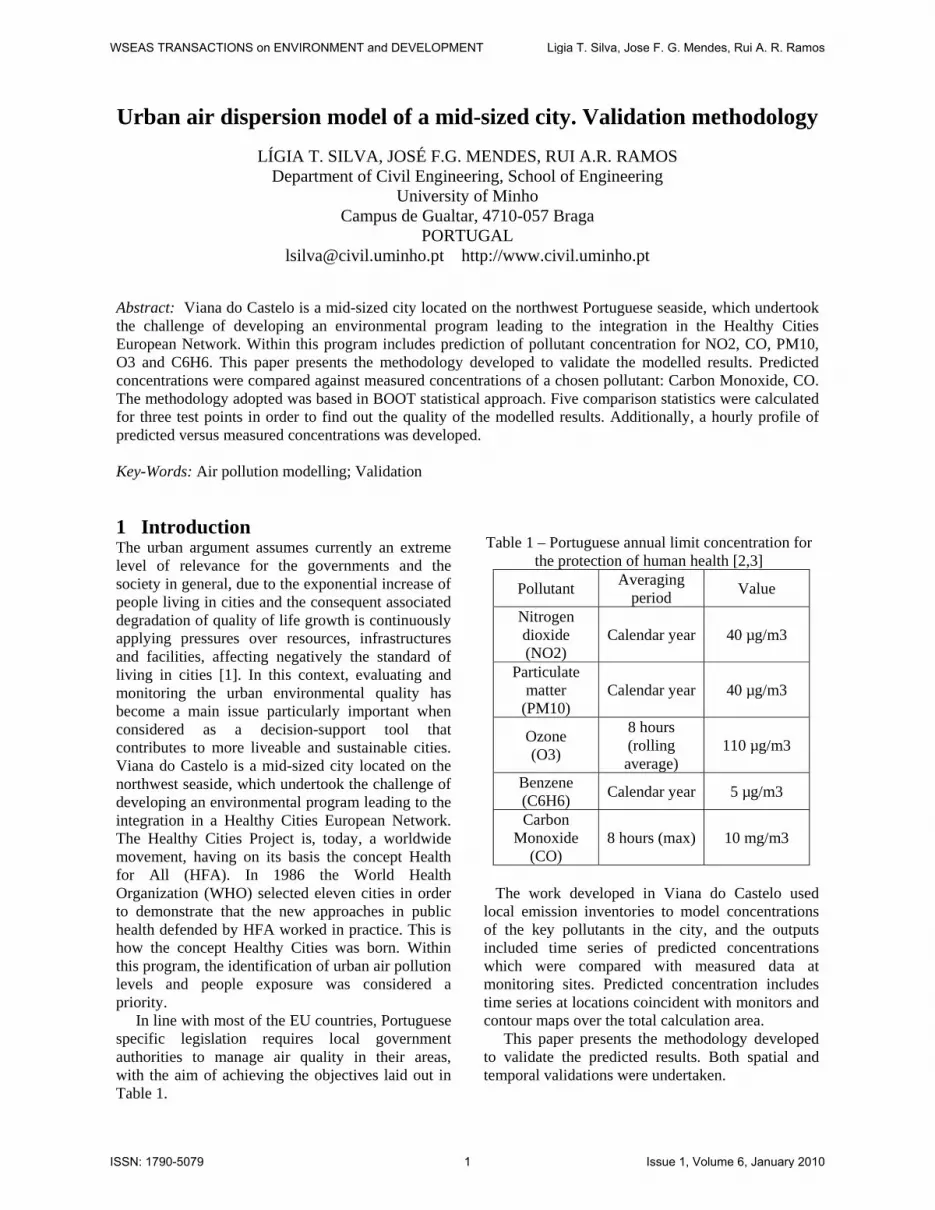
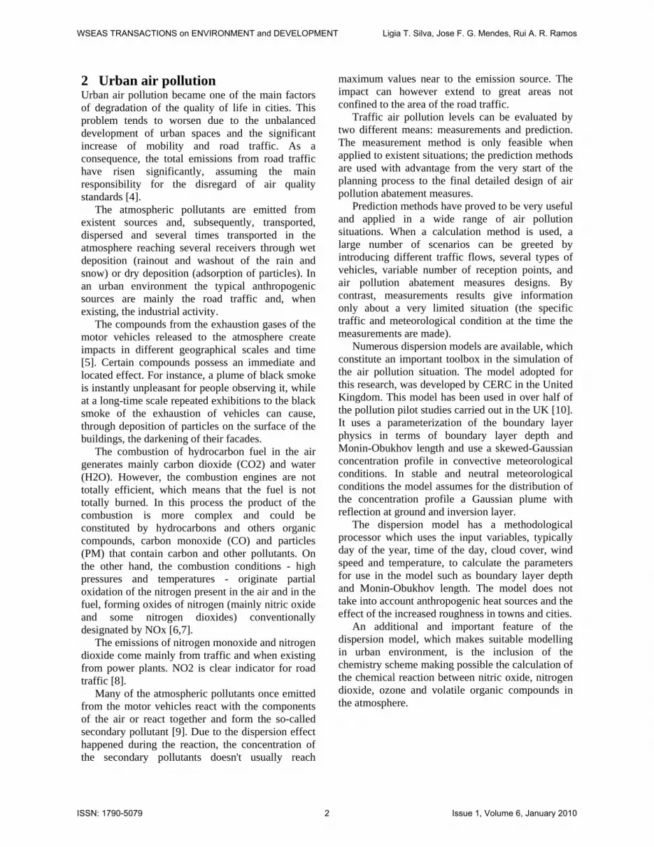
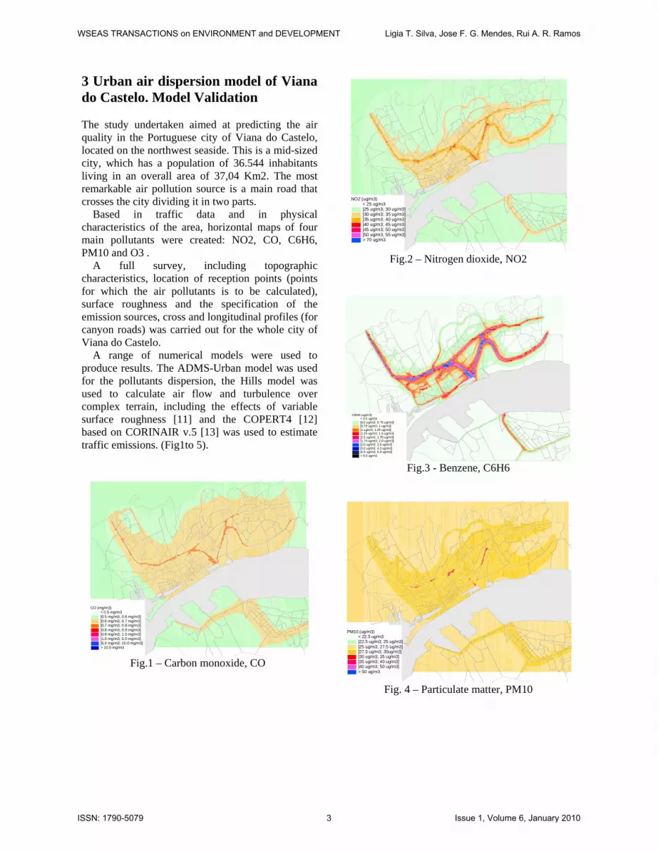
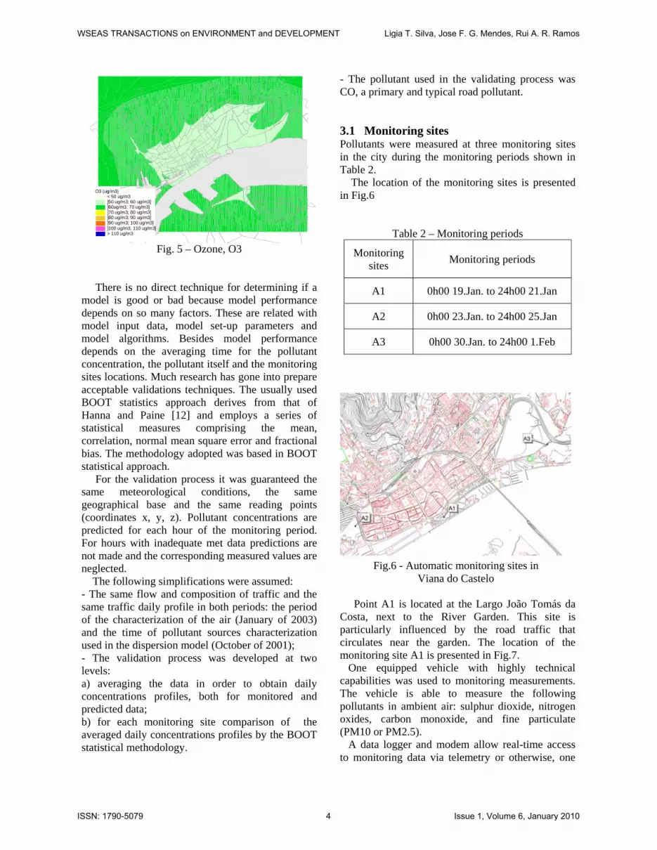
3 Urban air dispersion model of Viana do Castelo. Model Validation The study undertaken aimed at predicting the air quality in the Portuguese city of Viana do Castelo, located on the northwest seaside. This is a mid-sized city, which has a population of 36.544 inhabitants living in an overall area of 37,04 Km2. The most remarkable air pollution source is a main road that crosses the city dividing it in two parts. Based in traffic data and in physical characteristics of the area, horizontal maps of four main pollutants were created: NO2, CO, C6H6, PM10 and O3 . A full survey, including topographic characteristics, location of reception points (points for which the air pollutants is to be calculated), surface roughness and the specification of the emission sources, cross and longitudinal profiles (for canyon roads) was carried out for the whole city of Viana do Castelo. A range of numerical models were used to produce results. The ADMS-Urban model was used for the pollutants dispersion, the Hills model was used to calculate air flow and turbulence over complex terrain, including the effects of variable surface roughness [11] and the COPERT4 [12] based on CORINAIR v.5 [13] was used to estimate traffic emissions. (Fig1to 5).
Fig. 5 – Ozone, O3 There is no direct technique for determining if a model is good or bad because model performance depends on so many factors. These are related with model input data, model set-up parameters and model algorithms. Besides model performance depends on the averaging time for the pollutant concentration, the pollutant itself and the monitoring sites locations. Much research has gone into prepare acceptable validations techniques. The usually used BOOT statistics approach derives from that of Hanna and Paine [12] and employs a series of statistical measures comprising the mean, correlation, normal mean square error and fractional bias. The methodology adopted was based in BOOT statistical approach. For the validation process it was guaranteed the same meteorological conditions, the same geographical base and the same reading points (coordinates x, y, z). Pollutant concentrations are predicted for each hour of the monitoring period. For hours with inadequate met data predictions are not made and the corresponding measured values are neglected. The following simplifications were assumed: - The same flow and composition of traffic and the same traffic daily profile in both periods: the period of the characterization of the air (January of 2003) and the time of pollutant sources characterization used in the dispersion model (October of 2001); - The validation process was developed at two levels: a) averaging the data in order to obtain daily concentrations profiles, both for monitored and predicted data; b) for each monitoring site comparison of the averaged daily concentrations profiles by the BOOT statistical methodology.
- The pollutant used in the validating process was CO, a primary and typical road pollutant. 3.1 Monitoring sites Pollutants were measured at three monitoring sites in the city during the monitoring periods shown in Table 2. The location of the monitoring sites is presented in Fig.6
Table 2 – Monitoring periods
Monitoring sites Monitoring periods
A1 0h00 19.Jan. to 24h00 21.Jan
A2 0h00 23.Jan. to 24h00 25.Jan
A3 0h00 30.Jan. to 24h00 1.Feb
Fig.6 - Automatic monitoring sites in
Viana do Castelo Point A1 is located at the Largo João Tomás da Costa, next to the River Garden. This site is particularly influenced by the road traffic that circulates near the garden. The location of the monitoring site A1 is presented in Fig.7. One equipped vehicle with highly technical capabilities was used to monitoring measurements. The vehicle is able to measure the following pollutants in ambient air: sulphur dioxide, nitrogen oxides, carbon monoxide, and fine particulate (PM10 or PM2.5). A data logger and modem allow real-time access to monitoring data via telemetry or otherwise, one
WSEAS TRANSACTIONS on ENVIRONMENT and DEVELOPMENT Ligia T. Silva, Jose F. G. Mendes, Rui A. R. Ramos
ISSN: 1790-5079 4 Issue 1, Volume 6, January 2010
month of electronic data storage where data is downloaded manually at the site. The carbon monoxide was analyzed by Ambient CO Monitor with the following measurement principle: Non-dispersive Infrared (NDIR), according EN :14626.
Fig.7 – Point A1
Point A2 is located in the Campo do Castelo, a large square where some outdoor activities take place. The location of the monitoring site A2 is presented in Fig.8.
Fig.8 – Point A2
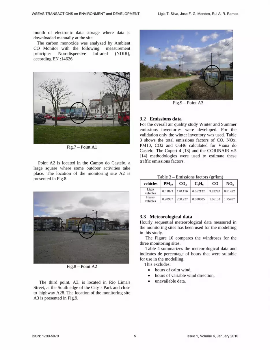
The third point, A3, is located in Rio Lima's Street, at the South edge of the City’s Park and close to highway A28. The location of the monitoring site A3 is presented in Fig.9.
Fig.9 – Point A3
3.2 Emissions data For the overall air quality study Winter and Summer emissions inventories were developed. For the validation only the winter inventory was used. Table 3 shows the total emissions factors of CO, NOx, PM10, CO2 and C6H6 calculated for Viana do Castelo. The Copert 4 [13] and the CORINAIR v.5 [14] methodologies were used to estimate these traffic emissions factors.
Table 3 – Emissions factors (gr/km) vehicles PM10 CO2 C6H6 CO NOx
Heavy vehicles 0.20997 250.227 0.000685 1.66133 1.75497
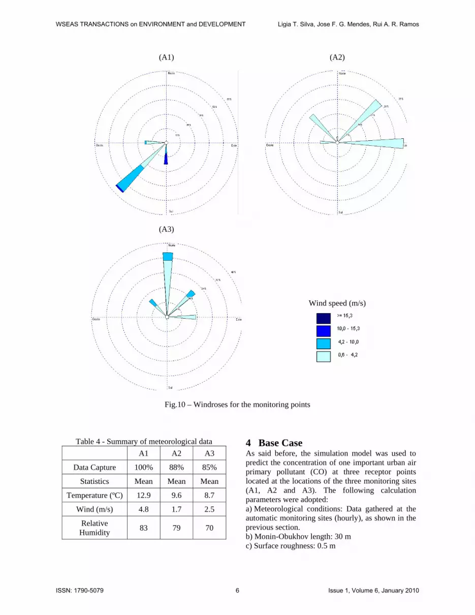
3.3 Meteorological data Hourly sequential meteorological data measured in the monitoring sites has been used for the modelling in this study. The Figure 10 compares the windroses for the three monitoring sites. Table 4 summarizes the meteorological data and indicates de percentage of hours that were suitable for use in the modelling. This excludes:
• hours of calm wind, • hours of variable wind direction, • unavailable data.
WSEAS TRANSACTIONS on ENVIRONMENT and DEVELOPMENT Ligia T. Silva, Jose F. G. Mendes, Rui A. R. Ramos
ISSN: 1790-5079 5 Issue 1, Volume 6, January 2010
(A1)
(A2)
(A3)
Wind speed (m/s)
Fig.10 – Windroses for the monitoring points
Table 4 - Summary of meteorological data A1 A2 A3
Data Capture 100% 88% 85%
Statistics Mean Mean Mean
Temperature (ºC) 12.9 9.6 8.7
Wind (m/s) 4.8 1.7 2.5
Relative Humidity 83 79 70
4 Base Case As said before, the simulation model was used to predict the concentration of one important urban air primary pollutant (CO) at three receptor points located at the locations of the three monitoring sites (A1, A2 and A3). The following calculation parameters were adopted: a) Meteorological conditions: Data gathered at the automatic monitoring sites (hourly), as shown in the previous section. b) Monin-Obukhov length: 30 m c) Surface roughness: 0.5 m
WSEAS TRANSACTIONS on ENVIRONMENT and DEVELOPMENT Ligia T. Silva, Jose F. G. Mendes, Rui A. R. Ramos
ISSN: 1790-5079 6 Issue 1, Volume 6, January 2010
d) Emissions inventory: database prepared for Viana do Castelo including road sources and industrial sources (Table 3). e) Background file: annual average background concentration of CO in the city [15]. f) Average speed: variable Main and secondary roads were modelled explicitly, as were major point industrial sources. One single profile was developed to represent the hourly variation of traffics flows on all the roads. 5 Validation 5.1 Statistics used Statistics calculated include mean, standard deviation, normalised mean square error, normalised bias and the FAC2. The data format was hour-by-hour for the measured concentrations (Xm, t=1, 2,… n) and predicted concentration (Xp, t=1, 2,… n), where t is the time in hours. The mean or average of the measured period mX
and pX . The Standard deviation, which is a measure of the dispersion of measured (Equation 1) and predicted concentrations (Equation 2).
( ) 2122
mmm XX −=σ (1)
( ) 2122
ppp XX −=σ (2)
The Normalised mean square error (NMSE), Equation 3, which is a normalized overall measure
of the error in hour-by-hour comparisons between measured and predicted concentrations. An exact data match would give a error of zero.
( )pm
pm
XXXX
NMSE2−
= (3)
Fractional bias (FB), Equation 4, which is a measure of the difference between the calculated average and the observed average. FB=0 indicates no difference, FB>0 indicate an underestimate in predicted concentrations and FB<0 indicate an overestimate.
( ) 2pm
pm
XXXX
FB+−
= (4)
The FAC2, which is the fraction of data that satisfy and must be within the following interval:
0.25.0 ≤≤m
p
CC
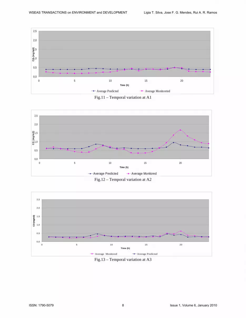
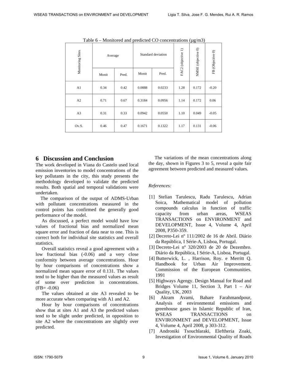
A perfect model would have FAC2=1.0, NMSE=0.0 and FB=0.0. 5.2 Comparisons between measured and modelled concentrations Figures 11, 12 and 13 compare the predicted and observed (monitored) average daily concentrations of CO at the monitoring sites A1, A2 and A3. Table 6 present statistics of comparisons between measured concentrations and ADMS-Urban calculations. Statistics have been calculated based on hourly comparisons for each site (A1, A2 and A3) and for overall statistics (Ov.S.).
WSEAS TRANSACTIONS on ENVIRONMENT and DEVELOPMENT Ligia T. Silva, Jose F. G. Mendes, Rui A. R. Ramos
ISSN: 1790-5079 7 Issue 1, Volume 6, January 2010
0,0
0,5
1,0
1,5
2,0
2,5
0 5 10 15 20Time (h)
CO
(mg/
m3)
Average Predicted Average Monitoreted Fig.11 – Temporal variation at A1
0,0
0,5
1,0
1,5
2,0
2,5
0 5 10 15 20Time (h)
CO
(mg/
m3)
Average Predicted Average Monitored Fig.12 – Temporal variation at A2
0,0
0,5
1,0
1,5
2,0
2,5
0 5 10 15 20
Time (h)
CO
(mg/
m3)
Average Monitored Average Predicted Fig.13 – Temporal variation at A3
WSEAS TRANSACTIONS on ENVIRONMENT and DEVELOPMENT Ligia T. Silva, Jose F. G. Mendes, Rui A. R. Ramos
ISSN: 1790-5079 8 Issue 1, Volume 6, January 2010
Table 6 – Monitored and predicted CO concentrations (µg/m3)
Mon
itorin
g Si
tes
Average Standard deviation
FAC
2 (o
bjec
tive
1)
NM
SE (o
bjec
tive
0)
FB (O
bjec
tive
0)
Monit Pred. Monit Pred.
A1 0.34 0.42 0.0888 0.0233 1.28 0.172 -0.20
A2 0.71 0.67 0.3184 0.0956 1.14 0.172 0.06
A3 0.31 0.33 0.0942 0.0550 1.10 0.049 -0.05
Ov.S. 0.46 0.47 0.1671 0.1322 1.17 0.131 -0.06
6 Discussion and Conclusion The work developed in Viana do Castelo used local emission inventories to model concentrations of the key pollutants in the city, this study presents the methodology developed to validate the predicted results. Both spatial and temporal validations were undertaken. The comparison of the output of ADMS-Urban with pollutant concentrations measured in the control points has confirmed the generally good performance of the model. As discussed, a perfect model would have low values of fractional bias and normalized mean square error and fraction of data near to one. This is correct both for individual site statistics and overall statistics. Overall statistics reveal a good agreement with a low fractional bias (-0.06) and a very close conformity between average concentrations. Hour by hour comparisons of concentrations show a normalized mean square error of 0.131. The values tend to be higher than the measured values as result of some over prediction in concentrations. (FB= -0.06) The values obtained at site A3 revealed to be more accurate when comparing with A1 and A2. Hour by hour comparisons of concentrations show that at sites A1 and A3 the predicted values tend to be slight under predicted, in opposition to site A2 where the concentrations are slightly over predicted.
The variations of the mean concentrations along the day, shown in Figures 3 to 5, reveal a quite fair agreement between predicted and measured values. References: [1] Stelian Tarulescu, Radu Tarulescu, Adrian
Soica, Mathematical model of pollution compounds calculus in function of traffic capacity from urban areas, WSEAS TRANSACTIONS on ENVIRONMENT and DEVELOPMENT, Issue 4, Volume 4, April 2008, P350-359.
[2] Decreto-Lei nº 111/2002 de 16 de Abril. Diário da República, I Série-A, Lisboa, Portugal.
[3] Decreto-Lei nº 320/2003 de 20 de Dezembro. Diário da República, I Série-A, Lisboa, Portugal.
[4] Butterwick, L. , Harrison, Roy. e Merritt Q. Handbook for Urban Air Improvement. Commission of the European Communities. 1991
[5] Highways Agengy. Design Manual for Road and Bridges Volume 11, Section 3, Part 1 – Air Quality, UK, 2003
[6] Akram Avami, Bahare Farahmandpour, Analysis of environmental emissions and greenhouse gases in Islamic Republic of Iran, WSEAS TRANSACTIONS on ENVIRONMENT and DEVELOPMENT, Issue 4, Volume 4, April 2008, p 303-312.
[7] Androniki Tsouchlaraki, Eleftheria Zoaki, Investigation of Environmental Quality of Roads
WSEAS TRANSACTIONS on ENVIRONMENT and DEVELOPMENT Ligia T. Silva, Jose F. G. Mendes, Rui A. R. Ramos
ISSN: 1790-5079 9 Issue 1, Volume 6, January 2010
in Heraklion, Crete, WSEAS TRANSACTIONS on ENVIRONMENT and DEVELOPMENT, Issue 12, Volume 4, December 2008, p 1120-1140.
[8] Maria Apascaritei, Francisc Popescu, Habil Ioana Ionel, Air pollution level in urban region of Bucharest and in rural region, Proceedings of 11th WSEAS International Conference on Sustainability in Science Engineering (SSE’09), Timisoara, Romania, May 27 - 29, 2009, p.330
[9] Silva, L.T., Mendes, J.F.G. Determinação do índice de qualidade do ar numa cidade de média dimensão. Engenharia Civil. 27 , p. 63-74, 2006
[10] Carruthers, D.J., Edmunds, H. A., Lester, A.E., McHugh, C. A. and Singles,. R. J. Use and Validation of ADMS-Urban in Contrasting Urban and Industrial Locations, Int. J. Environment and Pollution, Vol. 14, 364-374, 1998
[11] CERC, ADMS-Urban User Guide, Version 1.6, 2001
[12] S.R. Hanna Paine. Hybrid Plume Dispersion Model (HPDM) development and evaluation. J. Appl. Meteorol., 28, 206-224. 1989.