
1
A Seasonal Perspective on Regional Air Quality in Central
California
Shaheen R. Tonse, Lawrence Berkeley National Laboratory
CCOS Technical Committee MeetingSacramento, April 12, 2006

2
Team Members
• LBNL/UCB: Nancy Brown, Robert Harley, Ling Jin, Xiaoling Mao, Shaheen Tonse
• NOAA: JianWen Bao, Sara Michelson, Jim Wilczak

3
Research Objectives
• Use CMAQ with stateoftheart emissions, meteorological, and chemical inputs to model ozone in Central California for summer 2000
• Estimate how regional control strategy options for both 1hour, 120 ppb, and new 8hour, 80 ppb ozone standards change with respect to time and location
4
Task StructureOverview
• Task 1 – Develop modeling protocol
• Task 2 – Prepare model inputs2.1 Meteorological2.2 Emissions
• Task 3 – Conduct AQ modeling
• Task 4 – Model results analysisEvaluate analysis methodsDiagnose pollutant responses to precursors

5
Task 2.2: Emissions Inventory Development
Emission files:
CARB (area, biogenic, point, fire)UC Berkeley (motor vehicle, biogenic)
Provided on 190x190 grid with 4 km resolution
Hourly temporal resolution
Chemically speciated into SAPRC99
6
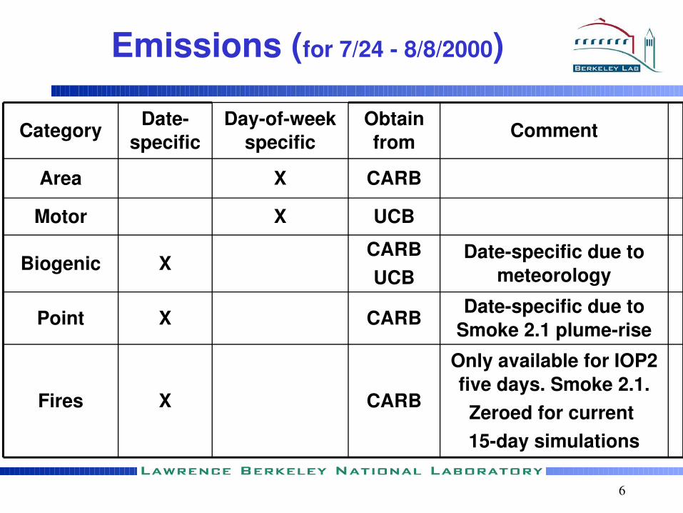
Emissions (for 7/24 8/8/2000)
Only available for IOP2 five days. Smoke 2.1.Zeroed for current 15day simulations
CARBXFires
Datespecific due to Smoke 2.1 plumeriseCARBXPoint
Datespecific due to meteorology
CARBUCB
XBiogenic
UCBXMotor
CARBXArea
CommentObtain from
Dayofweek specific
DatespecificCategory

7
Task 3: Air Quality Modeling
•CMAQ V4.5 air quality model
•Simulation detailsDomain and resolutionInputs (meteorology, emissions, boundary and initial conditions)
Computational detailsLBNL Linux ClusterCPU times and memory requirementsEstimates for 120 day run

8
CMAQ V4.5 (2005)
•Parallelized, F90, Linux, faster than CMAQ V4.3•Chemistry:
SAPRC99 chemistryEuler Backward Iterative (EBI) solverSmvgear stiff solver
•Improved advection results in better mass conservation•Improved vertical diffusivity algorithm
9
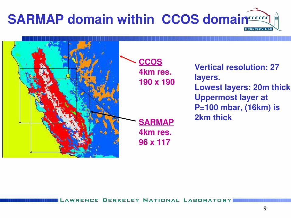
SARMAP domain within CCOS domain
CCOS4km res.190 x 190
SARMAP4km res.96 x 117
Vertical resolution: 27 layers. Lowest layers: 20m thickUppermost layer at P=100 mbar, (16km) is 2km thick

Initial and Boundary Conditions
2.52.5Aldehydes
0.70OLE1+2
12.57ALK1+2
40 7022 70O3
11NO2
0.050.05NO
200200CO
Other BCWestern BCSpeciesSelected boundary concentrations (in ppb)
Initial condition files are created by 72 hour spinup runs using the appropriate boundary conditions and dayofweek specific emissions

Computational Details
The “Mariah” Linux Cluster
• Provided by DOE
• Maintained by LBNL under the Scientific Cluster Support Program.
• 24 nodes, (2 processors and 2GB RAM per node)
• Centos Linux (similar to Red Hat Linux), run in a Beowulfcluster configuration

12
Computational Details
• Split the grid 3 ways in each direction and use 9 processor elements (PE’s):
• Current runtimes (96x117 domain):5day run takes 48 hours with Gear solver5day run takes 6 hours with EBI solver
• Projected seasonal runtimes (190x190 domain):120 day run (EBI) will take 461 hours (19 days)This can be accomplished in 70 hours by x8 splitting
of the simulation period

13
Memory Requirements
15 species51GB120190x190Output Concentration
180GB120190x190Emissions
204GB120190x190Meteorological
15 species2GB1596x117Output Concentration
7GB1596x117Emissions
8GB1596x117Meteorological
CommentSizedaysGridFile

14
Spatial distribution of O3 normalized bias
Sac
Fresno
#: < 15%#: 15 to 15%#: > 15%
cutoff at 25%

15
15day ozone time series (north central coast)
Jul24Jul24 Jul27Jul27 Jul30Jul30 Aug02Aug02 Aug05Aug05 Aug08Aug08
Episode

16
15day ozone time series (Livermore)
Jul24Jul24 Jul27Jul27 Jul30Jul30 Aug02Aug02 Aug05Aug05 Aug08Aug08
Episode

17
15day ozone time series (SJV)
Jul24Jul24 Jul27Jul27 Jul30Jul30 Aug02Aug02 Aug05Aug05 Aug08Aug08
Episode

18
Task 4: Model Results Analysis
• Large emphasis on analysis tools used in concert
• Statistical toolsPhysics analysis workstation (PAW), time series
analysis, clustering of modeling results
• Sensitivity AnalysisDDM for emissions, boundary conditions, initial
condition
• Process Analysis

19
5day Diagnostic Simulations
•Effect of different versions: CMAQ V4.3, V4.4, V4.5•Met. diagnostics
Nudged vs. unnudgedAveraged met. wind fields vs. instantaneous
•Other diagnosticsTitration: compare to O3+NO2 Coastal overestimation of O3:
O3 deposition to ocean?Effects of changing boundary conditions?Light attenuation
Photochemistry albedo effects

20
Night time Ozone Titration: O3+NO → NO2
Red: Observations Black: Model predictions
O3
O3 + NO2
21
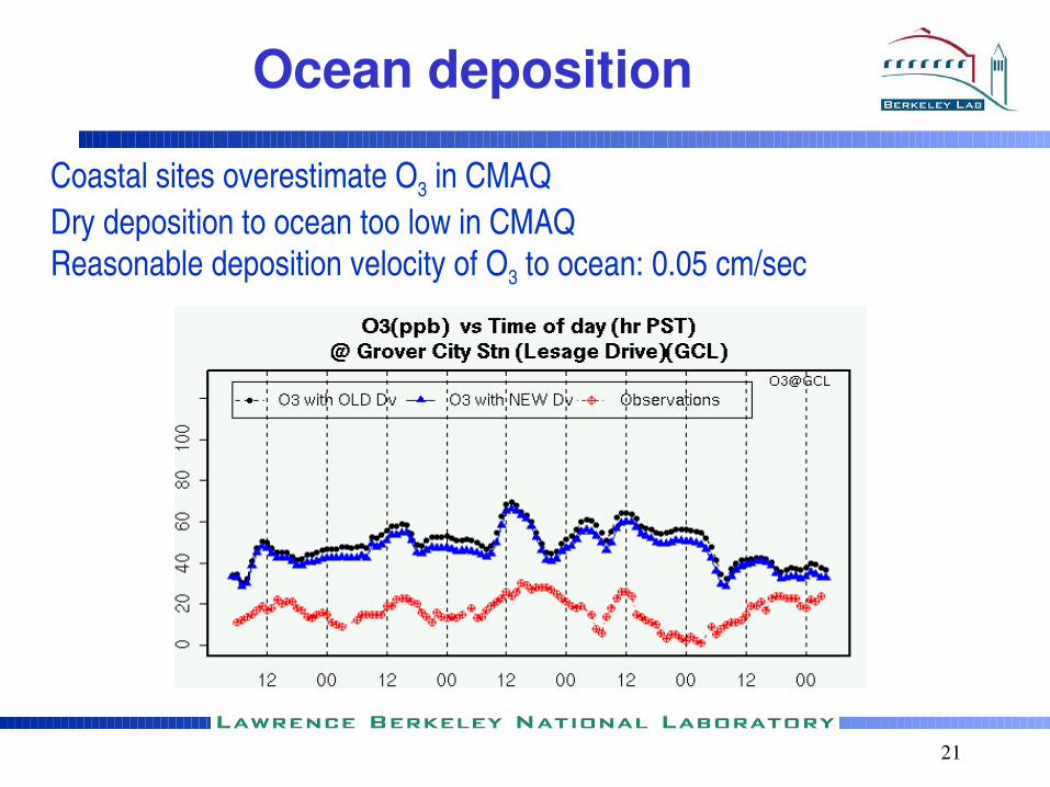
Ocean deposition
Coastal sites overestimate O3 in CMAQDry deposition to ocean too low in CMAQReasonable deposition velocity of O3 to ocean: 0.05 cm/sec
22
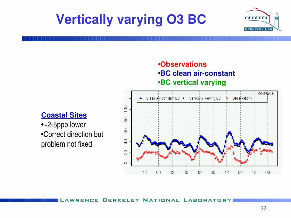
Vertically varying O3 BC
Coastal Sites•~25ppb lower•Correct direction but problem not fixed
•Observations •BC clean airconstant•BC vertical varying
23
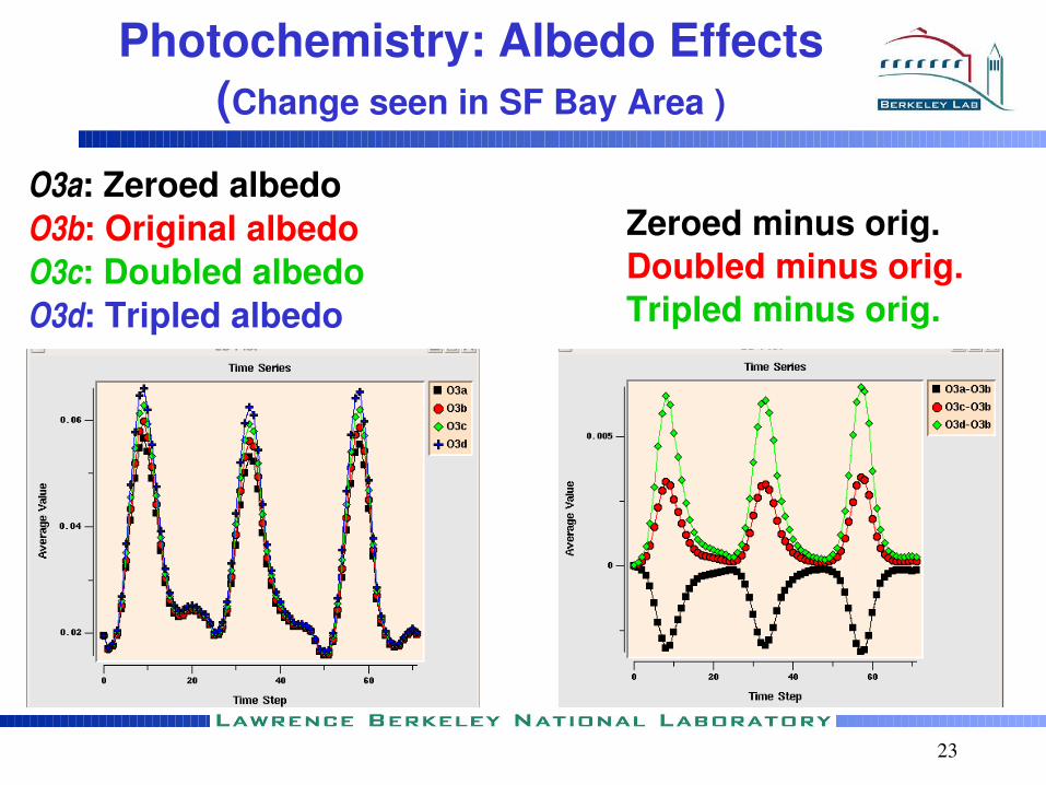
Photochemistry: Albedo Effects (Change seen in SF Bay Area )
O3a: Zeroed albedoO3b: Original albedoO3c: Doubled albedoO3d: Tripled albedo
Zeroed minus orig.Doubled minus orig.Tripled minus orig.

24
Attenuation of light in coastal stratus
Hourly CIMIS solar radiation (W/m2) measurements near Monterey Bay, 7/20 8/20/2000. (1 curve per day)
11am 7th Aug 2000

25
Sensitivity Analysis CMAQ DDM V4.3
5day and 15day runs of :dO3/d(NOx), dO3/d(AVOC), dO3/d(BVOC)
w.r.t boundary, initial conditionsw.r.t. emissions from selected regions or full domainw.r.t. timeofday of emissions from selected region
Following slides show seminormalized sensitivities: first derivative extrapolated to predict ozone as if 100% change in denominator value
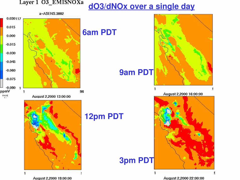
dO3/dNOx over a single day
6am PDT
9am PDT
12pm PDT
3pm PDT

27
dO3/dNOx at 3pm PDT on 3 successive days

28
dO3/d(AVOC) at 3pm PDT on 3 successive days

29
Combine analysis methods: DDM and PAW
For shaded region, compare O3 sensitivities to emissions from specific regions: SF Bay Area and Sacramento for a prolonged period.
Following plots present O3 sensitivities for the 12 noon – 4pm period for all 15 days
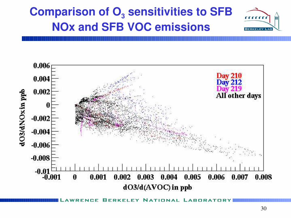
30
Comparison of O3 sensitivities to SFB NOx and SFB VOC emissions

31
Comparison of O3 sensitivities to SFB NOx and Sac. NOx emissions
32
Summary
Conducted and evaluated CMAQ 15 day simulations
Diagnosing model performancePhotochemistry: Albedo, cloud attenuationModel performance on coast
Sensitivity and other analysis tools used in concert can help classifying day’s meteorology when large data set available


![Bulb Eater Mercury Emissions Report - Air Cycle...0.05 (Skin) [6.1 ppb] 10.0 [1,219 ppb] 0.08 [9.8 ppb] 0.02 [2.4 ppb] Table Abbreviations and Notes ACGIH American Conference of Governmental](https://static.documents.pub/doc/80x56/5f322f109a7a2a0d8978f029/bulb-eater-mercury-emissions-report-air-cycle-005-skin-61-ppb-100-1219.jpg)
