

A Uni�ed Theory of Bond and Currency Markets
Andrey Ermolov∗
Columbia Business School,
Finance and Economics Division
October 8, 2014
Abstract
I show that an external habit model augmented with a heteroskedastic consumption
growth process reproduces main domestic and international bond market puzzles, consid-
ered di�cult to replicate simultaneously. Domestically, the model generates an upward
sloping real yield curve and realistic violations of the expectation hypothesis. Depending
on the parameters, the model can also generate a downward sloping real yield curve and
predicts that the expectation hypothesis violations are stronger in countries with upward
sloping real yield curves. Internationally, the model explains violations of the uncovered
interest rate parity. Unlike a standard habit model, the model simultaneously features
intertemporal smoothing to match domestic term structure and precautionary savings to
reproduce international predictability. The model also replicates the imperfect correla-
tion between consumption and bond prices/exchange rates through positive and negative
consumption shocks a�ecting habit di�erently. Mechanisms of the model are empirically
supported.
Keywords: �xed income, yield curve, expectation hypothesis, uncovered interest rate
parity, habit, time-varying volatility
JEL codes: E43, G12, G15
∗Uris Hall 8Q, 3022 Broadway, 10027 New York, NY, United States of America, (+1) 917-969-0060. This paper greatly
bene�ted from comments by Andrew Ang, Naveen Gondhi (TADC discussant), Robert Hodrick, Gur Huberman, Serhiy
Kozak (MFA discussant), Neng Wang, Andrés Ayala, Guojun Chen, Andrea Kiguel, Zhongjin Lu, and discussions with
Geert Bekaert and Lars Lochstoer. I also thank conference participants at the 2014 Midwest Finance Association meeting
and 2014 LBS Transatlantic Doctoral Conference for several insightful remarks. All errors are my own.

1 Introduction
Bond markets present both domestic and international puzzles. In the United States the
real yield curve is upward sloping and the expectation hypothesis is violated: the high
slope of the yield curve predicts high returns on the long-term bonds over the life of
short-term bonds. 1 At the same time, for instance, in the United Kingdom, the real
yield curve is downward sloping and the expectation hypothesis is not violated: the high
slope of the yield curve predicts low, instead of high, returns on the long term bonds over
the life of short-term bonds. Internationally, the uncovered interest rate parity seems
to be violated: a high di�erential between foreign and domestic interest rates strongly
predicts high returns on borrowing in domestic bonds and investing in foreign bonds.
This paper shows that a simple consumption based term structure model is able to ex-
plain the phenomena above. Replicating both domestic and international bond dynamics
within the same simple model is appealing, because most existing models explaining do-
mestic bond markets produce counterfactual implications internationally, likewise most
models addressing international bond markets produce counterfactual implications do-
mestically. As modern domestic and international bond markets are closely integrated,
this inability to explain them jointly constitutes one of the major puzzles in theoretical
asset pricing.
The proposed model is a habit model. In habit models the utility of an agent is deter-
mined by the di�erence between the current and habitual consumptions. The habitual
consumption (habit) is an aggregate of the past consumption history, which varies slowly
over time. As the �uctuations in the di�erence between the current and habitual con-
sumptions are percentually larger than �uctuations in the absolute consumption, in habit
models the agent is more sensitive to consumption shocks than in models where the util-
ity is determined by �uctuations in the absolute consumption alone (e.g., CRRA-utility
based models). The key di�erence to standard habit models (Abel 1990; Cambpell and
Cochrane, 1999) is that the model in this paper features a heteroskedastic consumption
growth process. This can be interpreted as a time-varying amount of risk. At the same
time, in contrast to the recent habit models (Campbell and Cochrane, 1999, Wachter,
1For instance, if the di�erence between the yields on 5 years and 1 year Treasury bonds is high, the
1 year return on holding a 5 years bond has historically been relatively high in US.
1

2002, Verdelhan, 2010), the price of risk in the model is constant. I show that, unlike the
standard habit speci�cation, my speci�cation allows to simultaneoulsy have intertermpo-
ral smoothing e�ect to match domestic term structure and precautionary savings e�ect
to reproduce international bond market dynamics.
The main puzzles explained by the model are di�erent slopes of the real yield curve,
violations of the expectation hypothesis and violations of the uncovered interest rate
parity. In the model, the average slope of the real yield curve is determined in the
interaction between the intertemporal smoothing e�ect and the precautionary savings
e�ect. If the intertemporal smoothing dominates: in times of low consumption the agent
wants to consume more and not save, thus, the bond prices will be low. As a result, long-
term bonds are a poor hedge against consumption shocks and should earn a premium
against the short-term bonds: the real yield curve slopes upwards. If the precautionary
savings e�ect dominates, in times of high consumption volatility the agent wants to save,
thus, bond prices will be high. Consequently, long-term bonds are a good hedge against
consumption volatility shocks and (assuming the agent dislikes volatility), should trade
at a discount against the short-term bonds: the real yield curve slopes downwards.
The violation of the expectation hypothesis is an observation that holding returns on long-
term bonds over the life of short-term bonds are high when the slope of the yield curve
is high. Thus, there are two parts in the expectation hypothesis: a time-varying slope
of the yield curve and time-varying returns on long-term bonds versus short-term bonds.
Theoretically, the slope of the yield curve consists of two components: the expected
change in the short rates in the future and the risk premium on holding a long term
bond over the life of the short-term bond. The �rst term corresponds to the fact that
if in the future short-term rates are expected to increase, the slope of the yield curve is
higher. The second term corresponds to the fact that holding a long-term bond over a
short period of time is risky because, until the payo� date, its price will �uctuate, and
these �uctuations might be correlated with investors' marginal utility. Consequently, if
investors require a compensation for holding a long-term bond over a short period of
time because of these �uctuations, the yield on the long-term bond will be relatively high
increasing the slope of the yield curve.
In the model, violations of the expectation hypothesis arise because an increase in the
2

consumption growth volatility increases the risk premium on holding a long term bond
over the life of a short-term bond. This requires that the intertemporal smoothing is
the dominant e�ect over precautionary savings. Indeed, if the intertemporal smoothing
dominates, in times of low consumption the agent wants to consume instead of saving.
This decreases the bond prices. Consequently, long-term bonds are a bad protection
against conusmption shocks and thus the required risk premium for holding them is high
when the magnitude (volatility) of these shocks is high. As explained above, this risk
premium is the second component of the slope of the yield curve. Thus, the increase in
this risk premium also increases the slope of the yield curve. Consequently, the slope of
the yield curve positively predicts returns on long-term bonds over the life of short-term
bonds.
Finally, in the model, violations of the uncovered interest parity are the result of the
the time-varying consumption growth volatility. The strategy of borrowing in country
1 and lending in country 2 is a poor hedge against the consumption shocks in country
1. To see this, suppose that a bad consumption shock realizes in country 1. The con-
sumption in country 1 becomes relatively scarce. Consequently, the agent who exchanges
country 2's consumption for country 1's consumption will receive relatively little of coun-
try 1's consumption when she needs it the most (after negative consumption shocks).
Because the strategy is a poor hedge against consumption shocks, the higher the mag-
nitude (volatility) of these shocks, the higher premium the agent requires. Note that
the higher consumption volatility in country 1 both decreases the interest rate in that
country through the precautionary savings motive and increases the expected return on
the strategy above.
The model in this paper addresses several problems of the main term-structure models:
the classic habit model, a long-run risk model, and a rare-disaster model. In particular,
the model is able to simulateneously replicate three major bond market puzzles: an
upward sloping real yield curve, violations of the expectation hypothesis, and violations
of the uncovered interest rate parity. The classic habit model by Wachter (2006) closely
replicates US bond market dynamics: in particular, an upward sloping real yield curve
and violations of the expectation hypothesis. However, a critique towards that model
(Verdelhan, 2010, Bansal and Shaliastovich, 2013) is that the uncovered interest rate
3

parity still holds. Additionally, the e�ective coe�cient of risk-aversion of 30 in the model
is relatively high. Verdelhan (2010) proposes an alternative habit model which is able to
explain the violations of the uncovered interest rate parity. However, in his model the
real yield curve is downward sloping and the expectation hypothesis holds. Thus, it is
not consistent with US bond markets. Additionally, in Verdelhan (2010) there is a strong
correlation between the exchange rate changes and the consumption growth di�erentials,
which is not the case in the data.
I also present a habit model. The main contribution over the previous habit-based term
structure models is showing the importance of time-varying volatility in consumption
growth for bond prices. Introducing a heteroskedastic consumption growth process into
a habit model leads to the separation of the intertemporal smoothing and precautionary
savings e�ects and thus allows to simultaneously match key domestic and international
bond market puzzles. 2 Under my speci�cation, the e�ective coe�cient of risk-aversion
is constant and is below 10 (which Mehra and Prescott, 1985, refer as an upper bound
of realistic values and which is low compared to the previous habit literature), and the
correlation between the exchange rate changes and the consumption growth di�erentials
is weaker than in Verdelhan (2010).
A long-run risk model (Bansal and Shaliastovich, 2013) is able to simultaneously explain
return predictability in domestic and international bond markets. Nevertheless, some of
the model's implications are not completely clear. First, the long-run risk framework
generally implies a downward sloping yield curve. Empirically, some countries (e.g., US)
have an upward sloping real yield curve. Additionally, long-run risk models rely on the
negative correlation between the consumption growth and in�ation and/or the expected
consumption growth and the expected in�ation to generate an upward-sloping nominal
yield curve. Such negative correlation has been observed in US during the twentieth
century. However, Hasseltoft and Burkhardt (2012) and Fleckenstein, Longsta�, and
Lustig (2013b) show that for the past decades this has not necessarily been the case. At
the same time, the nominal yield curve still remained mostly upward sloping during this
2Heyerdahl-Larsen (2012) and Stathopoulos (2012) start from a constant mean homoskedastic endow-
ment processes and are able to generate some time variation in the mean and volatility of consumption
growth through international trade, but this is not enough to su�ciently replicate bond returns pre-
dictability in either domestic or international markets (or both).
4

most recent period.
Second, in Bansal and Shaliastovich (2013) the real yield curve is downward sloping and
the expectation hypothesis is strongly violated. However, anecdotal evidence suggests
that countries with downward sloping real yield curves feature relatively weak violations
of the expectation hypothesis (UK).3The model in this paper generates, depending on
the parameters, both upward- and downward sloping real yield curves. Furthermore, the
model predicts that the expectation hypothesis violations are stronger in countries with
upward sloping yield curves.
At the �rst glance rare-disaster models (Farhi and Gabaix, 2010; Gabaix, 2012; Tsai,
2013) provide a good �t for both domestic and international bond market dynamics.4
The main problem is that they heavily rely on the extremely low consumption growth
outcomes not observed in many developed countries. Furthermore, in rare-disaster mod-
els, the real yield curve is either downward sloping or �at. In this paper extreme con-
sumption outcomes are not needed to reproduce the observed asset pricing dynamics. In
addition to the downward or �at real yield curves, the model in this paper can also have
an upward sloping real yield curve.
The paper also makes two methodological contributions into the habit literature. First,
I show that a heteroskedastic habit model allows to disentangle intertemporal smooth-
ing from precautionary savings e�ects, unlike standard homoskedastic habit models (e.g.,
Abel 1990, 1999; Campbell and Cochrane, 1999; Wachter, 2002; Verdelhan, 2010). In that
sense, the paper extends the heteroskedastic habit literature started by Bekaert (1996),
who only analyze international bond markets, and Bekaert and Engstrom (2009), who
only analyze basic asset pricing moments, such as the levels of the risk-free rate and the
equity premium. The result has implications for the speci�cation of habit models. Cur-
rently, there are two main speci�cations. The �rst and the most widespread speci�ciation
is with i.i.d. consumption growth shocks and the habit's time-varying sensitivity to these
shocks. This is approach taken, for instance, by Campbell and Cochrane (1999), Wachter
3This critique generally applies to the most long-run risk models trying to explain the US bond market
dynamics such as, for example, Hasseltoft (2012).4Gabaix (2012) and Tsai (2013) do not explicitly analyze international puzzles but back-of-the-
envelope calculations show that their models are able to address some of the international phenomena
such as violations of the UIP.
5

(2002), and Verdelhan (2010) and can be interpreted as a time-varying price of risk and a
�xed amount of risk approach. The second approach proposed by Bekaert and Engstrom
(2009) features heteroskedastic consumption growth shocks and the habit's constant sen-
sitivity to these shocks. This approach can be interpreted as a time-varying amount of
risk and a �xed price of risk approach. Verdelhan (2010) argues that the �rst approach
is not able to simultaneously explain US bond market dynamics and violations of the
uncovered interest rate parity. I show that the second approach is able to address this
task (due to the separation of the intertemporal smoothing from precautionary savings)
and thus appears to be more general. Additionally, an advantage of the time-varying
amount of risk is its computational simplicity: all solutions are available in closed form.
At the same time, solving external habit models with a time-varying price of risk usually
requires computationally heavy numerical procedures on a high precision grid (Wachter,
2005).
Second, I provide a potential explanation for why the consumption and asset prices are
relatively weakly correlated in data (e.g., Backus and Smith, 1993, for the international
�nance case). I �nd empirical evidence suggesting that positive and negative consumption
shocks a�ect habit di�erently. In particular, the intertemporal smoothing e�ect seems to
be driven exclusively by negative consumption shocks. In habit models prices are deter-
mined by both habit and the consumption growth. If habit is imperfectly correlated with
consumption (that is, for instance, negative consumption shocks a�ect habit di�erently
than positive shocks), then the prices will be imperfectly correlated with consumption as
well.
2 Bond and Currency Market Puzzles
This section provides qualitative and quantitative evidence on the real yield curve and its
slope, the expectation hypothesis and the uncovered interest rate parity across countries.
6

2.1 Slope of the Real Yield Curve
Slope of the real yield curve is the di�erence between interest rates on long-term real bonds
and short-term real bonds. Are these rates di�erent? Although the trading history of
in�ation adjusted bonds in the US is relatively short (starting from 1997), Piazzesi and
Schneider (2007) document that the real yield curve seems to be upward sloping. As
time passes by, there accumulates more support for this conclusion. For instance, taking
monthly US in�ation adjusted rates from January 2004 to August 2013 from the extended
appendix of Gurkaynak, Sack, and Wright (2009), the average di�erence between the 5
years yield and the 2 years yield is 0.41% (0.77% versus 0.36%) and is signi�cant at the
1% signi�cance level. A concern is that there are some liquidity issues in trading the
in�ation adjusted bonds in US (Fleckenstein et.al. 2013a). However, the slope is still
economically large and statistically signi�cant.
Although the trading of in�ation adjusted bonds in the US has started only in 1997,
several studies suggest that the average slope of the US real yield has been positive for
a long time. These studies extract the real yield cruve from the nominal yield curve,
in�ation forecasts, and estimates of the in�ation risk premium. For example, Chernov
and Mueller (2012) show that the average di�erence between the 5 years and the 1 years
real yields in US has been around 0.30% from 1971 to 2002. Ang and Ulrich (2012)
estimate that the average di�erence between the 10 years and the 5 years US real yields
has been around 0.45% from 1982 to 2008.
Internationally, there is also evidence of downward sloping real yield curves. For UK,
Evans (1998) and Piazzesi and Schneider (2007) document a downward sloping yield
curve: the di�erence between the 5 years yield and the 1 year yield is -0.30% (0.32%
versus 0.62%).
Unfortunately, the further international evidence on the slope of the real yield curve is
very limited, because in�ation adjusted bonds are issued in relatively few countries and
issues are mostly irregular and not very liquid (see Appendix A in Fleckenstein, 2013, for
a good overview of international in�ation adjusted bonds markets). Among a very few
studies concentrating on the international real yield curves, Ejsing et.al. (2007) document
that the real yield curve for France and Germany has been either �at or upward sloping.
7
Overall, it is puzzling why the real yield curve is upward sloping in some countries (US)
and downward sloping in others (UK).
2.2 Expectation Hypothesis
The expectations hypothesis (EH) states that all variation in long-term risk-free rates is
due to the variation in the future short-term risk-free rates. Informally, this means that
if the slope of the yield curve is high, the short-term rates in the future are expected to
rise and so will the yields on long-term bonds. Consequently, according to this theory,
holding long-term bonds for the lifetime of short-term bonds when the slope of the yield
curve is relatively high should result in relatively low returns.
Econometrically, the expectation hypothesis can be tested in several ways. In this paper,
I follow the approach of Campbell and Shiller (1991)5. They run the following regression
on the yields:
yn−1,t+1 − yn,t = β0 + βn1
n− 1(yn,t − y1,t) + εt, (1)
where y is the logarithmic yield, n is the number of periods to maturity, and t is the
time index. The expectation hypothesis implies that coe�cients βi should be equal to
1. However, Campbell and Shiller (1991) �nd that the coe�cients are negative and
decreasing with bonds maturities. This pattern has hold over time. Using the nominal US
government bonds from June 1960 to June 2013, the coe�cient in regression is gradually
decreasing from -0.75 for the two years bonds to -1.57 for the �ve years bond (using the 1
year bond as the reference). Thus, the expectation hypothesis is violated. Economically,
this means that long-term bonds deliver high, instead of low, returns when the slope of
the yield curve is high.
Interestingly, the expectation hypothesis holds quite well for UK bonds. For instance,
for regression (17) Bansal and Shaliastovich (2013) report positive regression coe�cients
which approach 1 at longer horizons.
5Another popular approach is as in Fama and Bliss (1987).
8

2.3 Uncovered Interest Rate Parity
Uncovered interest rate parity (UIP) states that the di�erence in the risk-free rates be-
tween two countries should be equal to the expected change in the exchange rate between
the currencies of the countries. Economically, this means that an investor should not be
able to make pro�ts from borrowing in country 1, exchanging the currency, lending in
country 2, and then exchanging the currency back the next time period.
Econometrically, the UIP can be tested in the following way. Let et be the logarithm of
the real exchange rate (the number of country 1 real consumption units given for a country
2 real consumption unit) and de�ne ∆et+1 = et+1−et. Finally, let y1,t and y∗1,t be the real
interest rates in countries 1 and 2, respectively. Then, rFXt+1 = −y1,t + y∗1,t + ∆et+1 is the
return from the strategy of borrowing in country 1 and lending in country 2 mentioned
above. The UIP implies that in the regression:
rFXt+1 = α0 + αFX(y1,t − y∗1,t) + εt, (2)
the coe�cient αFX should be equal to 0. However, numerous studies starting from Hansen
and Hodrick (1980) have shown that the coe�cient is negative and often less than −1.
For instance, Backus, Foresi, and Telmer (2001) document that for the US dollar-British
pound pair the coe�cient is -1.84, for the US dollar-Japanese yen pair -1.71, and for the
US dollar-German mark pair -0.74. Thus, the UIP is violated.
The reported coe�cients are stable at the prediction horizons from 1 month to 1 year.
Some studies suggest that the UIP holds better at horizons longer than one year (Alexius,
2001, and Chinn and Meredith, 2004). However, this evidence is not conclusive (Bekaert,
Wei, and Xing, 2007). Economically, this means that borrowing in low-interest rate
countries and lending in high-interest rate countries generates pro�ts. This is a so called
carry trade strategy.
3 Model
The model belongs to the class of external habit models. The key di�erence to the
standard external habit models (Abel, 1990, 1999; Campbell and Cochrane, 1999) is that
9
consumption growth shocks are heteroskedastic (which corresponds to a time-varying
amount of risk in the economy) but the sensitivity of the habitual consumption to these
shocks is constant over time (which corresponds to a �xed price of risk).
I only model the real side of the economy. This is because including money and in�ation
does not add much economic intuition. Calibrations show that including a consumption
non-neutral in�ation process into the model somewhat improves the empirical �t.
Modeling only the real side of the economy implicitly assumes that violations of the
expectation hypothesis and uncovered interest rate parity are at least partially real phe-
nomena. This assumption is empirically justi�ed. Bansal and Shaliastovich (2007) in their
Table II report that in US the in�ation-adjusted expectation hypothesis violations are
weaker than nominal expectations hypothesis violations but are still economically strong,
statistically signi�cant, and follow the same time pattern. P�ueger and Viceira (2011)
document strong violations of the expectation hypothesis in in�ation-indexed bonds. Hol-
li�eld and Yaron (2003) estimate that the uncovered interest rate parity violations should
be attributed almost exclusively to real risks.
3.1 Preferences
A representative agent maximizes the expected utility:
E0
∞∑t=0
βt(Ct
Ht)1−γ
1− γ, (3)
where Ct is the consumption at time t and Ht is the exogenous habit level (habitual
consumption). The motivation for using the habit preferences in the model is that the
agent becomes sensitive to relatively mild fundamentals' �uctuations.
Unlike the most of the recent literature (Campbell and Cochrane, 1999; Wachter, 2002;
Bekaert and Enstrom, 2009; Verdelhan, 2010), I use the ratio habit utility instead of a
di�erence habit utility. This is done for two reasons. First, in the ratio habit the coe�cient
of risk-aversion is constant, γ, which allows to concentrate on the core mechanism of this
paper: the heteroskedasticity of the consumption process. Second, in the ratio habit
framework, the habit has a straightforward interpretation of being a weighted average of
past consumption shocks. The di�erence habit framework allows this interpretation only
10

after the approximation around the steady state. Other papers which employ the ratio
habit utility are, for instance, Abel (1990, 1999) and Chan and Kogan (2002). Generally,
as shown in the calibration section, all results in the paper can be replicated with the
di�erence habit.6
3.2 Fundamentals Dynamics
The logarithmic consumption growth, gt+1 = ln Ct+1
Ct, is a constant mean heteroskedastic
process:
gt+1 = g + εt+1, (4)
where g is a constant and εt+1 is a mean 0 heteroskedastic shock. In this paper, εt+1 is
modeled as a mixture of two demeaned gamma-distributed shocks, ωp,t+1 and ωn,t+1:
εt+1 = σcpωp,t+1 − σcnωn,t+1,
ωp,t+1 ∼ Γ(p, 1)− p,
ωn,t+1 ∼ Γ(nt, 1)− nt,
(5)
where p and nt are shape parameters of the gamma distributions. ωp,t+1 roughly corre-
sponds to the right tail and ωn,t+1 to the left tail of the consumption growth distribution.
Economically, the consumption shock in the model has two components: one coming from
a good regime (ωp,t+1) and another coming from a bad regime (ωn,t+1).
Gamma distributions are used instead of more standard Gaussian distributions for purely
quantitative, not qualitative, reasons. Indeed, all main theoretical results in the paper
can be straightforwardly replicated with heteroskedastic Gaussian consumption shocks,
εt+1 ∼ N (0, σt). However, as it will be discussed in the calibration section, quantitatively
matching predictability patterns observed in the data is much easier with gamma dis-
tributed shocks. This is because gamma shocks have fatter tails than Gaussian shocks.
Thus, they increase the sensitivity of the agent to the shocks, which makes matching
asset prices easier. It should be also pointed out that gamma shocks are not simply a
6In fact, the calibration results with the di�erence habit are even stronger than with the ratio habit,
as the countercyclical risk-aversion ampli�es the asset pricing dynamics.
11

fancy technical tool but are empirically well justi�ed: Bekaert and Engstrom (2009) show
that gamma shocks describe the consumption dynamics better than Gaussian shocks.
At the �rst glance, the model might look like a rare disaster model but it turns out not to
be the case. In equation (5) the right tail has a constant shape while the shape of the left
tail varies over time. This indeed reminds a time-varying probability/size of a disaster
dynamics as, e.g., in Gabaix (2010) or Tsai (2013). However, in the calibration the
probability of an extreme consumption growth outcome in the model is very low: much
lower than in actual US data and by magnitudes lower than in rare disaster models. In
the model, the time-varying shape parameter of the left tail is used to model the time-
varying volatility of the consumption growth: the volatility of the ωn,t+1 shock is indeed
nt.7 Thus, instead of a rare disaster model a more appropriate title for the model is a
habit model with time-varying volatility of the consumption growth. Consistently with
this logic, in the remainder of the paper, I will refer to nt and p as to the volatility
parameters.
The shape parameter of the ωn,t+1 shock follows a lag 1 autoregressive process:
nt+1 = n+ ρn(nt − n) + σnnωn,t+1. (6)
The role of the state variable nt, corresponding to the time-varying volatility of the
consumption, is to determine the strength of the precautionary savings e�ect.
In equations (5) and (6) the negative shock to the consumption growth and the shock
to the volatility are the same. This corresponds to the observation that the volatility is
higher during recessions.
Finally, in line with the earlier work on the external habit formation, for the brevity of
exposition, I choose to model the logarithm of the consumption-habit ratio, st = ln Ct
Ht
instead of the habit itself. Similarly to the previous literature, the logarithm of the
consumption-habit ratio follows a lag 1 autoregressive process:
st+1 = s+ ρs(st − s) + σspωp,t+1 + σsnωn,t+1. (7)
7It is also possible to make the right tail of the consumption growth distribution time-varying. This
is not implemented for parsimony. Calibrations show that a model with a time-varying right tail instead
of a time-varying left tail performs quantitatively approximately as well as a model with time-varying
left tail, although the predictability patterns are weaker and fundamentals more volatile.
12

Under this speci�cation, the habit has an economically appealing interpretation of being
a weighted average of past consumption shocks. To see this, note that lnHt = gt − st =
g+σcpωp,t−σcnωn,t− s− ρs(st− s)−σspωp,t−σsnωn,t.. Plugging the process st from (7),
the habit is lnHt = constant+∑∞
i=0(αpiωp,t−i+αni ωn,t−i), where αpi and α
ni are constants.
The di�erence habit utility allows this interpretation only as an approximation around
the steady state.
Similarly to Campbell and Cochrane (1999), the consumption growth and the consumption-
habit ratio in equation (7) are driven by the same shocks.8 However, equation (7) allows
positive and negative shocks to a�ect the habit in di�erent way than they a�ect con-
sumption: generally σsp and σsn are not linked to σcp and σcn. Quantitatively, this
assumption is only important for replicating the weak correlation between consumption
growth and asset prices: prices are a�ected by the habit which in this speci�cation is
not perfectly correlated with the consumption. All other moments can be approximately
reproduced from the model where the shock to the consumption growth and the shock to
the consumption-habit ratio are perfectly correlated (that is, σsp = ασcp and σsn = −ασcnfor a constant α > 0). However, in Section 5 I show that the assumption of positive and
negative consumption shocks a�ecting habit di�erently enjoys some empirical support
and thus it is justi�able to include it into the model. 9
Note that the consumption-habit ratio, st, in equation (7) plays a di�erent role than the
consumption-habit ratio in Campbell and Cochrane (1999). In my model, the role of st
is purely the intertemporal smoothing (determining how valuable is consumption today
compared to consumption in the future), the risk-aversion is constant. In Cambpell and
Cochrane (1999) the consumption-habit ratio, in addition to intertemporal smoothing,
8Cambpell and Cochrane (1999), Wachter (2002), Bekaert and Engstrom (2009), and Verdelhan
(2010) use the di�erence habit utility. For that reason, they are modeling the inverse surplus ratio
instead of the consumption-habit ratio. The inverse surplus ratio and the consumption-habit ratio are
technically di�erent speci�cations to model the economically same thing. Thus, to avoid the confusion
with terminology, in the paper I will refer to both of them as to the consumption-habit ratio.9A di�erent sensitivity to negative and positive shocks can be related to reference point-utility pref-
erences (Koszegi and Rabin, 2009), where bad consumption ouctomes hurt more than good consumption
outcomes bene�t. There is empirical evidence in favor of such preferences (Crawford and Meng, 2009,
Pope and Schweitzer, 2011, Sydnor, 2010, among others) and thus they are not simply a convenient
technical tool.
13

also determines the risk-aversion (which in their model is time-varying).
Economically, positive shocks should increase the consumption habit ratio and negative
consumption shocks should decrease the consumption-habit ratio (corresponding to the
situation where positive consumption shocks increase utility and negative consumption
shocks decrease it). Thus, σqp is expected to be negative and σqn is expected to be
positive.
The key di�erence between the model in this paper and the standard habit model by
Cambpell and Cochrane (1999) is that in this paper the consumption growth shocks are
heteroskedastic, but sensitivity of the agent's consumption-to-habit ratio to these shocks
is constant, in contrast in Campbell and Cochrane (1999) the consumption growth shocks
are homoskedastic, but sensitivity of the consumption-to-habit ratio to these shocks
is time-varying. This turns out to be very important because this paper's speci�ca-
tion allows to disentangle the intertemporal smoothing and precautionary savings ef-
fects from each other. Indeed, the intertemporal smoothing process is governed mainly
by the consumption-habit ratio process (7), while the precautionary savings are driven
by the volatility process (6). In the standard habit model (Campbell and Cochrane,
1999; Wachter, 2002; Verdelhan, 2010), there is no time-varying consumption volatility.
Both the intertemporal smoothing and precautionary savings e�ects are driven by the
consumption-habit ratio process. Depending on the speci�cation of that process, either
the intertemporal smoothing or the precautionary savings e�ect is dominant all the time.
This severely restricts term structure dynamics and, in particular, precludes explaining
domestic and international bond markets dynamics simultaneously: in Wachter (2002)
the intertemporal smoothing dominates and the uncovered interest rate parity holds,
while in Verdelhan (2010) the precautionary savings dominate and the real yield curve is
downward sloping and the expectation hypothesis holds. The model in this paper disen-
tangles the intertemporal smoothing and precautionary savings e�ects and allows them
to operate to some extent independently. As shown in the next section, this allows to
simultaneously match domestic and international bond market dynamics.
14

4 Asset Pricing Implications
This section explains how the model is able to generate bond market predictability pat-
terns often considered puzzling. To clarify economic intuition, I concentrate on the ex-
amples with one and two period bonds and then discuss how the results are generalized
for longer term bonds. All asset prices in the model are closed-form and thus easy to
interpret. For brevity, in this section I only discuss the formulas necessary for intuition.
All other equations are relegated to the appendix.
In line with the previous external habit literature, the agent only maximizes her utility
with respect to consumption and takes the habit as given. Consequently, the stochastic
discount factor, Mt+1, is equal to the ratio of marginal utilities of consumption at t + 1
and t:
Mt+1 = βCtCt+1
(Ct+1
Ht+1)1−γ
(Ct
Ht)1−γ = βe−gt+1+(1−γ)(st+1−st). (8)
Risk premia on the assets are determined by the covariance of their returns with the inno-
vations to the stochastic discount factor. The innovations to the (logarithmic) stochastic
discount factor are:
mt+1 − Etmt+1 = apωp,t+1 + anωn,t+1,
ap = (1− γ)σsp − σcp,
an = (1− γ)σsn + σcn.
(9)
For simplicity, I only consider the case where positive consumption growth shocks decrease
the stochastic discount factor (corresponding to good times) and negative consumption
growth shocks increase the stochastic discount factor (corresponding to bad times). In
(9), this corresponds to ap < 0 and an > 0.
4.1 Yield Curve
All bonds are real risk-free zero-coupon bonds. It is covenient to work with the continu-
ously compounded yields de�ned as:
yn,t = − 1
nlnPn,t, (10)
15

where t is the time index, n is the number of periods to the payo�, and P is the bond
price.
Let us �rst analyze the one period risk-free rate. Using the formulas for expectations of
gamma distributed variables from the appendix, (8) yields:
y1,t = − ln β + g − (1− γ)(1− ρs)s+ f(ap)p+ (1− γ)(1− ρs)︸ ︷︷ ︸<0
st + f(an)︸ ︷︷ ︸<0
nt, (11)
where:
f(x) = x+ ln(1− x). (12)
Note that in (12) function f(x) is always negative.
The risk-free rate in equation (11) consists of two components: the intertemporal smooth-
ing and precautionary savings. First, the risk-free rate loads negatively on the consumption-
habit ratio st.10 This is the intertemporal smoothing e�ect: in times of low consumption
(low st) the agent wants to consume now and not in the future and thus needs to be
compensated for transfering consumption into the future. Second, the risk-free rate loads
negatively on the consumption growth volatility nt. This is the precautionary savings
e�ect: in times of high consumption growth volatility (high nt) the agent wants to save
to hedge the uncertainty.
To understand how the average slope of the yield curve is determined, let us consider an
example with only one and two period zero-coupon bonds. The return on holding a two
period bond over one period is R2,t→t+1 = P1,t+1
P2,t. Taking logs:
r2,t→t+1 = −y1,t+1 + 2y2,t. (13)
Rearranging and taking unconditional expectations of (13) results in:
E(y2,t − y1,t) =1
2E(y1,t+1 − y1,t)︸ ︷︷ ︸
expected change in the short rate
+1
2E(r2,t→t+1 − y1,t)︸ ︷︷ ︸
risk-premium for holding a 2 period bond over 1 period
,
E(y2,t − y1,t) =1
2E(r2,t→t+1 − y1,t).
(14)
The left hand side of (14) is the average slope of the yield curve in our two bonds example.
In the �rst line it consists of two parts. The �rst part corresponds to the expected return
10Throughout the paper I assume that the risk-aversion coe�cient, γ, is greater than 1.
16

on holding a two period bond once the one period bond expires: from time t + 1 to
time t + 2. This correponds to the expected change in short rates. The second part is
the expected excess return on holding a two period bond over the life time of the one
period bond. Note that this return is not necessarily 0, because the two period bond is
only riskless at the two period horizon, at the one period horizon its price will �uctuate
and these �uctuations might be correlated with the agent's marginal utility (stochastic
discount factor). From the second line of (14), this risk-premium determines the average
slope of the yield curve. This is because on average the 1 period yields today and the
next period will be equal and thus the �rst term cancels out.
By de�nition, the risk-premium on holding a two period bond over 1 period, E(r2,t→t+1−
y1,t), is determined by the covariance of r2,t→t+1 with the stochastic discount factor:
E(R2,t→t+1 −Rft→t+1) = − cov(Mt+1R2,t→t+1)
EMt+1
11. In logs:
E(r2,t→t+1 − y1,t) ≈ −cov(mt+1, r2,t→t+1) = cov(mt+1, y1,t+1), (15)
where the �rst part is an approximation, because there is also a Jensen inequality term
due to the concavity of the logarithm function.
The logic behind (15) is that if a future short yield (y1,t+1) is positively correlated with
the stochastic discount factor holding a two period bond is risky. This is because if the
next period the stochastic discount factor will be high (a bad situation for the agent), the
short term yield is likely to be high as well, implying a low bond price. Consequently, the
agent needs to be compensated for holding a two period bond. From (14), this implies a
positive average yield curve slope.
In the model, the average slope of the yield curve is determined in the interaction of
the intertemporal smoothing and precautionary savings e�ects. To see this, note that
plugging (15) into (14) yields:
E(y2,t − y1,t) =1
2E(r2,t→t+1 − y1,t) ≈
1
2cov(mt+1, y1,t+1)
=
intertemporal smoothing, ∝covt(mt+1,st+1)︷ ︸︸ ︷−S1σsnanV ar(nt)︸ ︷︷ ︸
>0
+
precautionary savings, ∝covt(mt+1,nt+1)︷ ︸︸ ︷N1σnnanV ar(nt)︸ ︷︷ ︸
<0
,
11This follows from substituting the de�nition of the covariance into the de�niton of the stochastic
discount factor: E(Mt+1R2,t→t+1) = 1.
17

(16)
where the second line is computed by substituting in (9) and (11). The �rst term in (16)
is the intertemporal smoothing term, which comes from the covariance of the stochastic
discount factor with consumption-habit ratio. If a negative consumption shock is realized,
the consumption-habit ratio drops, increasing the short-term yield (equation (11)) and
consequently decreasing bond prices. Thus, a two period bond is a bad hedge against
consumption shocks and should trade at premium. Indeed, the �rst term in (16) is
positive.
The second term in (16) is the precautionary savings term, which comes from the covari-
ance of the stochastic discount factor with consumption growth volatility. If a negative
consumption shock is realized, the consumption growth volatility rises, decreasing the
short-term yield (equation (11)) and consequently increasing bond prices. Thus, a two
period bond is a good hedge against consumption shocks and should trade at discount.
Indeed, the second term in (16) is negative.
Overall, the slope of the yield curve will be determined by which of the two e�ects is
stronger:
1) Long-tem bonds are a poor hedge against the consumption shocks because they de-
crease the consumption-habit ratio decreasing bond prices. Thus, the real yield curve
should slope up.
2) Long-term bonds are a good hedge against the consumption shocks because they
increase the consumption growth volatility increasing bond prices. Thus, the real yield
curve should slope down.
For longer horizons, the model can reproduce a very rich set of real yield curves: upward-
sloping (as, e.g., for US in Gurkaynak, Sack, and Wright 2009), downward-sloping (as,
e.g., for UK in Piazzesi and Schneider, 2007), hump-shaped (as, e.g., for US in Ang,
Bekaert, and Wei, 2008), or U-shaped. This is because in the model the relative strength
of the intertemporal smoothing and precautionary savings e�ects are di�erent at di�er-
ent horizons: at some horizons the intertemporal smoothing e�ect might be dominant
increasing the slope of the yield curve, while at other horizons the precautionary savings
e�ect is dominant decreasing the slope of the yield curve.
18

4.2 Expectation Hypothesis
To understand the implications of the model for the expectation hypothesis, let us again
consider the two bonds example. Going back to equation (13), rearranging and taking
conditional expectations:
y2,t − y1,t︸ ︷︷ ︸slope of the yield curve
=1
2Et(y1,t+1 − y1,t)︸ ︷︷ ︸
expected change in the short rate
+1
2Et(r2,t→t+1 − y1,t)︸ ︷︷ ︸
risk-premium for holding a 2 period bond over 1 period
.
(17)
The left hand side of (17) is the time t slope of the real yield curve, which consists of two
parts. The �rst part corresponds to the expected relative return on holding a two period
bond once the one period bond expires: it is equal to the expected change in the short
rate. That is, if the expected change in the short rate next period, y1,t+1 − y1,t is high,
then the slope of the real yield curve is going to be high as well. This is consistent with
the expectation hypothesis: the high yield curve slope should predict high future short
rates and thus low returns on long-term bonds.
The second part of the time t slope of the real yield curve in equation (17) is the risk-
premium for holding a two period bond over the �rst period (that is over the life of the
one period bond). This risk-premium is not necessarily zero or even constant, because
the price of a two period zero-coupon bond next period is not sure: it will depend on the
short rate next period. Furthermore, this dependance might vary through time. As the
short rate next period might be correlated with the marginal utility (stochastic discount
factor) of the agent, there will be a premium (or a discount) for holding a two period
bond over one period.
The model explains violations of the expectation hypothesis via the time-varying volatility
of the consumption shocks. Suppose that the time t consumption growth volatility is
relatively high. The �rst component of the real yield curve in (17), the expected short
rate next period, is then relatively high as well. To see this, note that due to the mean-
reversion in the volatility (equation (6)), the volatility next period is expected to be lower.
Consequently, the precautionary savings e�ect is expected to be weaker and the expected
short interest rate is high (equation (11)).
If the intertemporal smoothing is the dominant e�ect, then the second component of the
19

real yield curve in (17), the risk-premium on holding a two period bond over one period,
is also high in times of high consumption growth volatility. To see this, let us analyze
the conditional version of equation (16):
Et(r2,t→t+1−y1,t) =
intertemporal smoothing, ∝covt(mt+1,st+1)︷ ︸︸ ︷−S1σsnanV art(nt+1)︸ ︷︷ ︸
>0
+
precautionary savings, ∝covt(mt+1,nt+1)︷ ︸︸ ︷N1σnnanV art(nt+1)︸ ︷︷ ︸
<0
.
(18)
From (6), V art(nt+1) is proportional to nt. If the intertemporal smoothing is the dominant
e�ect, in (18) the �rst term is more important and the risk premium on holding a two
period bond is high when the consumption growth volatility is high. The intuition is that,
as the two period bond is a bad hedge against consumption shocks, the agent should be
compensated more for holding it when the magnitude (volatility) of these shocks is large.
Thus, as both components of the slope of the real yield curve are high in times of high
consumption growth volatility, the slope is itself high in these times.
To summarize, assuming that the intertemporal smoothing is the dominant e�ect in the
model, the high consumption growth volatility drives up both the slope of the yield curve
and the holding returns on long-term bonds. Thus, the high slope of the yield curve
predicts high returns on the long-term bonds. The expectation hypothesis is violated.
Assuming that the precautionary savings is the dominant e�ect, the model can also
replicate the non-violated expectation hypothesis, as observed, for example, in UK. To
see this, note from (18) that, if the precautionary savings e�ect is the dominant e�ect, the
risk premium on holding a two period bond over one period is low when the consumption
growth volatility is high. The intuition is that, as the two period bond is a good hedge
against consumption shocks, the agent should be compensated less for holding it when
the magnitude (volatility) of these shocks is large. Thus, when the consumption growth
volatility is high, the �rst term in (17) will be high and the second term in (17) will be
low. Thus, depending on which of these two terms is more important, in times of the
high consumption growth volatility the slope of the real yield curve will be either high
or low and thus will be positively (the expectation hypothesis is violated) or negatively
(the expectation hypothesis holds) correlated with the expected return on holding a two
period bond over one period.
Comparing this and the previous subsection, note the link between the slope of the
20

real yield curve and the expectation hypothesis. If the intertemporal smoothing e�ect
is dominant, the yield curve is sloping up and the expectation hypothesis is likely to be
violated. At the same time, if the precautionary savings e�ect is dominant, the yield curve
is sloping down and the expectation hypothesis is more likely to hold. This prediction
is in line with the anecdotal two country evidence (US and UK) that the expectation
hypothesis holds better in countries with the downward sloping real yield curve.
In the model, the degree of the expectation hypothesis violations might vary at di�erent
time horizons (as is the case, for instance, in US data). This is because, depending on
the model's parameters, at each time horizon, the relative strength of the intertemporal
smoothing and precautionary savings e�ects might be di�erent.
4.3 Uncovered Interest Rate Parity
To understand the implications of the theory for the uncovered interest rate parity, let
us analyze the return, rFXt+1 , from borrowing in country 1 and lending the same amount
in country 2. I assume that there are two countries with one country speci�c consump-
tion good each.12 Following Backus et.al. (2001), Verdelhan (2010), and Bansal and
Shaliastovich (2013), I assume that �nancial markets are complete and there are no arbi-
trage opportunities. Under these assumptions, the exchange rate change is equal to the
di�erence in stochastic discount factors: ∆et+1 = m∗t+1 −mt+1. Thus:
EtrFXt+1 = −y1,t + y∗1,t + Et(m
∗t+1 −mt+1) = N1︸︷︷︸
>0
(nt − n∗t ). (19)
The intuition behind the return on the cross-country borrowing-and-lending strategy is
as follows. First, the return is independent of the consumption-habit ratio st. This is
because the role of st is intertemporal smoothing. Intertemporally, nothing changes for
the agent: she borrows in country 1 and lends the same amount in country 2, her time t
consumption is una�ected.
Second, the return is higher the higher is the volatility in country 1, nt. This is because the
12This assumption is in line with an empirical evidence by Burstein, Eichenbaum, and Rebelo (2006)
that most of the real exchange rate �uctuations are driven by non-tradable goods. Recall that, as shown
by Holli�eld and Yaron (2003), the real exchange rate �uctuations are the most relevant for the uncovered
interest rate parity violations.
21

strategy is a poor hedge against negative shocks, ωn,t+1, to the stochastic discount factor
and, thus, according to (9) should earn positive returns when the magnitude (volatility)
of these shocks (nt) is higher. To see why the strategy is a poor hedge against negative
shocks, suppose a large negative shock in country 1 realizes. Then the country 1's con-
sumption is scarce compared to the country 2's consumption. Consequently, the agent
who will be exchanging the country 2's consumption units for the country 1's consump-
tion units will get little consumption when she needs it the most (in the case of large
negative consumption shocks in country 1).
Note that the argument in the previous paragraph is a volatility, not a disaster, argument.
The strategy above is also a poor hedge against positive shocks, ωp,t+1. To see this,
suppose a large positive shock in country 1 realizes. Then the country 1's consumption
is abundant compared to country 2's consumption. Consequently, the agent who will
be exchanging the country 2's consumption units for the country 1's consumption units
will get a lot of consumption when she needs it the least (in the case of large positive
consumption shocks in country 1). Thus, the argment for the positive shock is the same
as for the negative shock. As already mentioned before, the time-varying volatility of
only the negative shock is a choice made mainly for the brevity of the exposition: the
logic of the model is replicable with time-varying volatility of positive shocks.
The model's explanation for the violations of the uncovered interest rate parity is based
on the fact that consumption growth volatility a�ects both the interest rate and the
return on the cross-country borrowing-and-lending stragegy at the same time. Indeed,
from (11) the interest rate is decreasing in volatility nt due to the precautionary savings.
From (19) EtrFXt+1 is in increasing in the volatility nt because the trading strategy is a poor
hedge against consumption shocks and thus is riskier when the magnitude (volatility) of
these shocks is higher. Thus, when the agent borrows from a low interest rate country
and invests into the high interest rate country, she has a large exposure to consumption
shocks in the low-interest rate country.13 Thus, on average, she should earn a premium
13In (11) the interest rate also depends on the consumption-habit ratio st. As st and nt are negatively
correlated, when nt is high, the risk-free rate might be relatively high, instead of low, due to the low st.
This would make the uncovered interest rate parity hold. However, quantitatively, in the economically
sensible parameter region, the impact of the st on the uncovered interest rate parity seems to be always
smaller than the impact of the volatility driven dependence discsussed in the main text.
22

from such a strategy.
4.4 Equity
Similarly to the previous habit literature starting from Campbell and Cochrane (1999),
the equity is modeled as the claim to the each period's consumption. The price-dividend
ratio is solved in closed form in the appendix by using the formulas for expectations
of gamma distributed variables. The solution and intuition for equity are largely from
Campbell and Cochrane (1999) and Bekaert and Engstrom (2009) and thus an interested
reader is referred to these papers for a detailed discussion.
5 Empirical Evidence and Simulation
I start by demonstrating empirical evidence in favor of main mechanisms driving the
model. Next, I show that under reasonable parameters the model is able to reproduce
bond and equity market dynamics in US and internationally, including di�erent slopes of
the yield curve, violations of the expectation hypothesis and the uncovered interest rate
parity. I also quantitatively demonstrate the link between the slope of the real yield curve
and the violations of the expectation hypothesis established in the previous section.
5.1 Empirical evidence
5.1.1 Domestic bond markets
In modeling the domestic term-structure, there are 3 key mechanisms in the model:
1) intertemporal smoothing: interest rates are low when the consumption-habit ratio is
high and interest rates are high when the consumption-to-habit ratio is low
2) precautionary savings: interest rates are low when the consumption growth volatility
is high and interest rates are high when the consumption growth volatility is low
3) di�erent sensitivity of the consumption-habit ratio to positive and negative consump-
tion shocks
23

The risk-free rate equation (11) is the key equation to empirically evaluate the mech-
anisms above. In particular, it states that the real risk-free rate should be decreasing
in the consumption-habit ratio and decreasing in the conditional consumption growth
volatility. These predictions can be tested by regressing a proxy for the real risk-free
rate on proxies for the consumption-habit ratio and the conditional consumption growth
volatility. Furthermore, the di�erent sensitivity of the consumption-habit ratio to positive
and negative shocks can be studied by constructing proxies for the consumption-habit
ratio where positive and negative shocks contribute di�erently and investigating if these
proxies are more successful in explaining asset prices than proxies where all consumption
shocks a�ect the consumption-habit ratio in the same way.
In order to test the mechanisms in data, I need a proxy for the real interest rate as well
as for the consumption-habit ratio and the consumption growth volatility. I approximate
the real interest rate by taking the nominal 3 month Treasury bill rate from the St.Louis
Fed website and reducing the expected in�ation for the next quarter from the Survey
of Professional Forecasters. I operate at the quarterly frequency, because ignoring the
in�ation risk premium is better justi�ed for short time intervals as the in�ation is strongly
predictable.The time period is 1969Q1-2012Q4, because the in�ation forecasts are not
available before that.
I approximate the consumption-habit ratio using its evolution process given in (7). First,
assume that the shock to the consumption-habit ratio is the the same as to the consump-
tion growth (mathematically, σsp = ασcp and σsn = −ασcn). Then, by iterating equation
(7) backwards, the consumption-habit ratio can be expressed as:
st = const+ α∞∑i=0
ρis(σcpωp,t−i − σcnωn,t−i). (20)
Note that, under the model's assumptions, shocks (σcpωp,t−i−σcnωn,t−i) in (20) are simply
consumption growth shocks and are thus directly observable from data. This allows to
approximate the consumption-habit ratio using the past consumption growth data. In
particular, Wachter (2002) argues that around 40 quarters of past consumption is needed
to approximate habit, and this is the value I use in this paper. ρs is set to 0.97 which
is the average quarterly habit persistence in the previous habit literature (Campbell and
Cochrane, 1999; Wachter, 2002, 2006; Verdelhan, 2010) and this paper.
24

The general speci�cation in equation (7) allows positive and negative components of
consumption growth shocks to a�ect the consumption-habit ratio in di�erent ways than
they a�ect consumption growth (mathematically, σsp = α1σcp and σsn = −α2σcn with
α1 6= α2). By iterating equation (7) backwards, the consumption-habit ratio can be
expressed as:
st = const+ α1
∞∑i=0
ρisσcpωp,t−i + α2
∞∑i=0
ρis(−σcnωn,t−i). (21)
Filtering σcpωp,t−i and −σcnωp,t−i for equation (26) from data is non-obvious. Thus, as a
�rst approximation, to simplify the computational burden, I set:
∞∑i=0
ρisσcpωp,t−i :=∞∑i=0
ρis(gt−i − g)1(gt−i−g)≥0,
∞∑i=0
ρis(−σcnωn,t−i) :=∞∑i=0
ρis(gt−i − g)1(gt−i−g)<0,
(22)
where 1 is an indicator function. The interpretation of equation (22) is that positive
components of the consumption growth shocks are simply estimated as the positive con-
sumption growth shocks, and negative components of the consumption growth shocks are
estimated as the negative consumption growth shocks. This is an approximation because
in the model every consumption growth shock is always a mixture of a positive and a
negative component (see equation (5)). As components follow a demeaned gamma dis-
tribution, ωp,t might well be negative and −ωn,t positive. In empirically evaluating (22),
I again follow the previous literature and use 40 quarters of data and ρs=0.97.
Finally, I estimate the conditional volatility of consumption growth using two di�erent
ways. First, I assume that the consumption growth follows a constant mean heteroskedas-
tic process, where the error term is following a GARCH(1,1) process. That is I estimate
the following process for the quarterly consumption growth data via maximizing the
likelihood:
gt = g + σtεt,
σ2t = σ + ρσσ
2t−1 + φ(gt−1 − g)2,
εt ∼ N (0, 1).
(23)
I employ σt in (23) as the �rst measure of the conditional volatility of the consumption
growth.
25

Note that (23) is an approximation because as equation (5) states the shocks in the
model are gamma and not normally distributed. To address this issue, I also compute
the conditional volatility using the gamma shocks. In particular, I estimate the follow-
ing BEGE-GARCH (Bekaert, Engstrom, and Ermolov, 2014) process for the quarterly
consumption growth data (again via maximizing the likelihood):
gt = g + σcpωp,t − σcnωn,t,
ωp,t ∼ Γ(p, 1),
ωn,t ∼ Γ(nt−1, 1),
nt = n+ ρnnt + φn(gt−1 − g)2,
(24)
I employ√σ2cpp+ σ2
cnnt−1 as the second measure of the conditional volatility of the
consumption growth. Note that (24) is still an approximation to the theoretical process
in the paper, because for computational reasons I do not �lter ωn,t and ωp,t shocks and,
thus, unlike in the theoretical model, the shock to the volatility (nt) does not equal the
ωn,tmshock to the consumption growth.
Table 1 illustrates that the model in this paper seems to be roughly consistent with US
data while previous habit models seem to be not. In particular, speci�cation 1 shows that
taken alone, a consumption-habit ratio seems to be positively (albeit statistically insignif-
icantly) associated with risk-free rates. This casts doubt on the traditional habit-based
explanation of an upward sloping real yield curve and the violations of the expectation
hypothesis (Wachter, 2006), as this explanation requires a negative relationship between
the consumption-habit ratio and short-term risk-free rates (in order for long-term bonds
to be risky securities).
Speci�cation 2 in Panel A of Table 1 shows that impact of positive and negative consump-
tion shocks on the consumption to habit ratio is indeed statistically signi�cantly di�erent
(the coe�cient of the Consumption-habit− is statistically signi�cantly negative). In par-
ticular, while for positive consumption shocks the relationship between the consumption-
habit ratio and risk-free rates is still positive (the coe�cient of the Consumption-habit is
positive), the relationship between the negative shocks and the consumption-habit ratio
becomes negative (0.5715-0.8452=-0.2737). This implies that empirically the intertem-
poral smoothing e�ect is pronounced for negative consumption shocks and is absent for
positive consumption shocks. Indeed, in data a large in magnitude negative shock to the
26

consumption-habit ratio leads to higher risk-free interest rates implying that bonds are
a bad hedge for consumption shocks. Interestingly, a large in magnitude positive shock
also implies higher risk-free rate. The results of speci�cations 1 and 2 in Panel A sug-
gest that in order to justify some kind of the intertemporal smoothing in data under the
habit framework, one should allow negative and positive consumption shocks to a�ect
the consumption-habit ratio di�erently.
Speci�cations 3 and 4 in Panel A of Table 1 show the evidence of the intertemporal
smoothing and precautionary savings e�ects in data. Speci�cation 3 shows that if posi-
tive and negative shocks are not allowed to a�ect the consumption-habit ratio di�erently,
there is no evidence of either intertemporal smoothing or precautionary savings e�ects.
Contrary, both the higher consumption-habit ratio and the higher conditional volatility of
the consumption growth are associated with the higher risk-free rates (coe�cients of the
Consumption-habit and Conditional volatility are positive). However, speci�cation 4 indi-
cates that if positive and negative shocks do a�ect the consumption-habit ratio di�erently
(and they do a�ect the consumption-habit ratio di�erently as the Consumption-habit−
coe�cient is statistically signi�cantly negative), there appears to be the intertemporal
smoothing e�ect for negative shocks (consistently with results in speci�cations 1 and 2)
and the precautionary savings e�ect (a negative coe�cient for the Conditional volatility).
Thus, in line with speci�cations 1 and 2, speci�cations 3 and 4 suggest that once posi-
tive and negative consumption shocks are allowed to a�ect the consumption-habit ratio
di�erently, there is evidence of both intertemporal smoothing and precautionary savings
e�ects. Results using gamma distributed shocks (in Panel B of Table 1) are in line with
results obtained with Gaussian shocks.
Overall, the empirical evidence suggests that the positive and negative consumption
shocks a�ect the consumption-habit ratio di�erently, and, after accounting for this,
there are intertemporal smoothing and precautionary savings e�ects.14 The intertem-
poral smoothing seems to be driven almost exclusively by negative shocks. Consistently
with this observation, in the calibration of the model negative consumption shocks will
have greater impact on the consumption-to-habit ratio than positive shocks.
14Importantly, this also adresses the Hartzmark (2014)'s empirical critique towards the absence of the
link between economic (consumption) growth and interest rates.
27

Table 1 about here.
5.1.2 International bond markets
Data supports the model's volatility based explanation for the uncovered interest rate
parity violations. From Panel A of Table 2 it can be seen that, in line with the model's
mechanism, the consumption growth volatilities for the low interest countries are higher
than for high interest countries.15 Panel B of Table 2 shows that the di�ferences are often
statistically signi�cant. Interestingly, the di�erences in consumption growth volatilities
are smaller in the most recent sample. This is largely in line with the observation that G10
carry trade returns have been economically relatively weak and statistically insigni�cant
in 1990:s and 2000:s (see, for example, Table 8 in Chabi-Yo and Song, 2013, for the most
recent evidence).
Table 2 about here.
5.2 Calibration
I calibrate the model to match the bond and equity markets dynamics in US. Interna-
tionally, I match the uncovered interest rate parity coe�cient observed between US dollar
and some common currencies. I calibrate the model at the annual frequency. This is to
avoid the time aggregation issues.
In the calibration, I aim to match the following set of moments:
a) US per capita consumption growth moments: mean, standard deviation, skewness, ex-
cess kurtosis, probabilities of extreme outcomes (<mean-2×standard deviation, <mean-
4×standard deviation). I obtain these moments from NIPA tables 1.1.6 (the real con-
sumption growth) and 7.1 (the population growth). The time period is 1929-2012.
b) US real interest rates: annual real interest rates for 1,2,3,4, and 5 years and the
volatility of the 1 year interest rate. This data is from the updated appendix of Gurkaynak
et.al. 2009 and covers the period from 2004 to 2012. The TIPS data is only available at
15Ready, Roussanov, and Ward (2014) report the same empirical evidence in the context of a di�erent
model.
28

annual maturities with the shortest maturity being 2 years. For this reason, I linearly
extrapolate the values for the 1 year real bonds from the 2,3,4, and 5 years bonds. The
time period is relatively short because the history of in�ation adjusted bonds trading in
US is short.
c) US equity: equity risk-premium, Sharpe-ratio, price dividend ratio. The risk-premium
and Sharpe-ratio are from Kenneth French's data library. The price-dividend ratio is
from Boudoukh et.al. (2007). The time period is 1929-2012. 16
d) US expectation hypothesis coe�cients for 2,3,4, and 5 years bonds using the 1 year
bond as a reference short-term security. The expectation hypothesis coe�cients are not
directly available for real bonds. Thus, I compute them by running regression (17) for
the nominal bonds. The data on the yields is from the updated appendix of Gurkaynak
et.al. (2006). I do not aim to match these coe�cients exactly, because I am operating
with real, not nominal, yields. I aim to match the negativity of the coe�cients and that
the coe�cients are more negative for the bonds with longer maturities.
e) The uncovered interest rate parity coe�cient between US and other major economies.
The uncovered interest rate parity coe�cients are not directly available in real terms
because there is not long enough history of real government bonds trading for the most
countries. The uncovered interest rate parity coe�cients are from Backus et.al. (2001).
The calibration is the mix of minimizing the weighted squared distance between the model
implied moments and their empirical counter-parts and the hand-calibration. I partially
rely on the hand calibration because it is not feasible to get consistent standard errors
for all the moments of interest: some moments are only available in nominal terms and
time periods for di�erent moments are rather di�erent. For the identi�cation purposes,
the discount factor β is �xed to 0.975. This is the average of the discount factors from
Campbell and Cochrane (1999) and Wachter (2002). The level of the consumption-habit
16Calibrating the price dividend ratio is somewhat complicated. In the model, the price-dividend ratio
corresponds to the equity payout ratio: that is the ratio of the equity price to the total payout (not only
dividends but also share repurchases and equity issuance). Boudoukh et.al. (2007) show that in recent
years this statistic has gone very small and even negative. This means that the capital have been �owing
from households to �rms. The model in this paper is not designed to have such negative dividends. Thus,
instead of the payout ratio I follow most of the asset pricing literature, such as Campbell and Cochrane
(1999) or Bansal and Yaron (2004), and match the price-dividend ratio from Boudoukh et.al. (2007).
29

ratio is set to 1. Unlike in the Campbell and Cochrane (1999)-type models, the level
of the consumption-habit ratio is irrelevant for pricing, because, as it can be seen from
equations (8) and (9), the stochastic discount factor is only dependent on the ratio (not
levels) of the consumption-habit ratios across di�erent time periods.17 Thus, s can have
an arbitrary positive value.
The parameters which will �t consumption and asset pricing dynamics reasonably well
are summarized in Table 3. The local relative risk-aversion (which is a rough counter-
part to the CRRA risk-aversion in the model) is relatively low compared to other models
which try to explain bond markets predictability such as Wachter (2002) and Bansal and
Shaliastovich (2013).The persistence of the habit might look low, but this is an annual
persistence, not monthly or quarterly persistence used in most other habit models. The
persistence of the habit is roughly in line with the annualized value from Bekaert and
Engstrom (2009). In line with economic intuition, positive consumption shocks increase
and the negative consumption shocks decrease the consumption-habit ratio. The left tail
of the consumption growth distribution is much stronger non-Gaussian than the right-
tail. This is consistent with US consumption dynamics analyzed in Bekaert and Engstrom
(2009). Figure 1 visualizes the consumption growth distribution in the model.
Table 3 about here.
Figure 1 about here.
5.3 Results
The model �ts both consumption and asset pricing dynamics reasonably well. Table
4 shows that the model implied consumption dynamics is more Gaussian than US con-
sumption in 1929-2012. The probability of the consumption disasters in the model is very
low compared to the rare disaster models: around 2% for the two standard deviations
disaster and almost 0 for the four standard deviastions disaster. For instance, in the rare
disaster literature, Gabaix (2012) requires the probability of the four standard deviation
17In the Campbell and Cochrane (1999)-type models, the level of the consumption-habit ratio is
important, because it a�ects the habit's sensitivity to consumption shocks. In this paper this sensitivity
is constant.
30

consumption growth disaster to be 3%. Additionally, in his model the disasters are very
severe, corresponding to around -30% annual consumption growth. This has never been
observed in US (although has been observed internationally). Tsai (2013) requires the
probability of the four standard deviations consumption growth disaster to be 1.8% per-
cent but in his model the consumption disasters can be signi�cantly larger than in Gabaix
(2013). 18 Thus, as already discussed, the model is not a rare disasters-type model.
Table 4 about here.
Table 5 demonstrates the model's ability to match the key asset pricing characteristics. In
particular, the model adresses a common critique towards the habit model regarding its
inability to simultaneously explain violations of the expectation hypothesis and uncovered
interest parity (Verdelhan, 2010; Bansal and Shaliastovich, 2013).
Table 5 about here.
Consistently with the data, the expectation hypothesis violations in the model are stronger
at the longer horizons (β-coe�cients in Table 5 decreasing over time). This is just the
consequence of the deep model parameters. In the calibration, the sensitivity of the yield
curve's slope to the consumption volatility is mainly determined by the habit and volatil-
ity persistence components, ρs and ρn. At the same time, the sensitivity of the long-term
bonds holding returns to the consumption volatility is mainly determined by the habit
sensitivity parameters, σsp and σsn. In order for β-coe�cients in Table 5 to decrease over
time, the parameters should be chosen so that holding returns on long-term bonds are
more sensitive to the consumption volatility than the slope of the yield curve. This is
doable because the slope and the holding returns are largely a�ected by di�erent model
parameters.
The expectation hypothesis coe�cients in the model are not decreasing as fast over time
as they do in the data. This might be partially attributed to the fact that the model is the
real model: non-neutral in�ation would apmlify the e�ects. It should also be pointed out
18In Nakamura et.al. (2013) the probability of the four standard deviation disaster is 1.12%, which is
in line with the twentieth century US data, but authors are not concerned about predictability patterns,
they only match basic asset pricing moments.
31

that in the long-run risk models such as Hasseltoft (2012) and Bansal and Shaliastovich
(2013) the time pattern in the expectation hypothesis coe�cients is also somewhat weaker
than in the data.19
Note that the volatility of the real interest rate in the model is realistically low. As
Cambpell and Cochrane (1999) point out, habit models usually generate too high in-
terest rate volatility. In this paper, this is not a problem because the intertemporal
smoothing and precautionary savings e�ects always drive the risk-free rate in opposite
directions reducing its �uctuations. For instance, if a large negative shock does realize, the
consumption-to-habit ratio goes down increasing the interest rate and the consumption
growth volatility goes up decreasing the interest rate.
The equity premium in the model is a little bit low compared to the data. At the same
time, the equity premium in the model is roughly consistent with the US equity premium
over the longer time period: for instance, for the period from 1889 to 1994 Campbell
et.al. (1997) in their Table 8.1 report the equity premium of 4.18%. The relatively low
equity premium is a general problem of the ratio-habit model (see, e.g., Chan and Kogan,
2002). In the next section I show that using the di�erence habit instead of ratio habit
addresses the low equity premium in my model.
An obvious problem with the model is that the exchange rate volatility is too high. This
corresponds to the observation by Brandt et.al. (2006) that it is di�cult to reconcile high
domestic Sharpe-ratios with the low exchange rate volatility. The reason is that to �t
the high domestic Sharpe-ratios the variance of the stochastic discount factors should be
high (Mehra and Prescott, 1985). However, the high volatility of the stochastic discount
factor implies high volatility of the exchange rates: V ar∆et+1 = V ar(mt+1)+V ar(m∗t+1)−
2ρ(mt+1,m∗t+1)
√V ar(mt+1)V ar(m∗t+1). In the habit framework, Verdelhan (2010) solves
this problem by introducing between the countries trading costs. This mechanism can
also be applied to this paper at the cost of losing the intuition provided by closed form
solutions.
19Hasseltoft (2012) uses a slightly di�erent method to test the expectation hypothesis and the time
pattern in the model is slightly weaker than in data. In Bansal and Shaliastovich (2013) the appropriate
comparision to this paper is the cross-country calibration in Table 7.
32

The model is to some extent able to match the non-perfect correlation between the ex-
change rate changes and consumption growth di�erentials. This weak correlation �rst
documented in Backus and Smith (1993) is theoretically often considered puzzling. In-
deed, Backus and Smith (1993) show that under the no-arbitrage condition in complete
markets with the CRRA utility, the exchange rate changes should be proportional to the
consumption growth di�erentials between two countries: ∆et+1 = −γ(g∗t+1− gt+1). Thus,
the exchange rate changes and the consumption growth di�erentials should be perfectly
correlated.
The habit model is usually able to match the low correlation between the exchange rate
changes and the consumptiong growth di�erentials better than CRRA-based models,
because the exchange rates are determined not only by the consumption growth but also
by the habit. However, as Verdelhan (2010) points out the correlation in habit models is
generally still too strong (around 0.75 in his model). In this paper the correlation between
the exchange rate changes and the consumption growth di�erentials is weaker than in the
previous habit models. This is because the shocks to the consumption growth and the
inverse surplus ratio are imperfectly correlated: ωn,t+1 and ωp,t+1 a�ect the consumption
and habit with di�erent weights.
Table 6 con�rms the theoretically predicted ability of the model to produce the downward
sloping yield curve along with "non-violated" expectation hypothesis. Note that the
main di�erence between the parameters in Tables 3 and 6 is the higher risk-aversion
and volatility in the later speci�cation. This makes sense, because, as discussed in the
previous section, in order for the yield curve to slope downward and the expectation
hypothesis to hold the precautionary savings e�ect should dominate. The result is also
indirectly supported empirically as historically the consumption growth volatility in UK
has been higher than in US.
Table 6 about here.
5.4 Role of Model Ingredients
In this section, I analyze two of the model's features which are di�erent from the main-
stream literature: using gamma shocks instead of Gaussian shocks and using the ratio
33

habit instead of the di�erence habit.
5.4.1 Gamma Shocks
The role of gamma shocks in this paper is largely quantitative, not qualitative. Indeed,
the logic of the model is easily replicapable with Gaussian shocks with time-varying
volatility.
However, calibrating the model with Gaussian shocks is much more challenging. In
particular, because gamma shocks have fatter tails than Gaussian shocks, volatility of
Gaussian shocks should be relatively high to generate the same amount of predictability
in asset prices. As it can be seen from Figure 1 and Table 4, the consumption growth
in the model is less volatile than US consumption growth in 1929-2012. With Gaussian
consumption shocks, the unconditional volatility of the consumption growth would be
somewhat higher than in 1929-2012 US in order to generate roughly the same amount of
predictability as reported in Tables 5 and 6. Additionally, the mean e�ective coe�cient
of risk-aversion would be around 20. It is important to emphasize that gamma shocks are
not just a convenient theoretical tool: they are empirically well justi�ed. For instance,
Bekaert and Engstrom (2009) show that gamma shocks match the consumption growth
dynamics (e.g., conditional consumption growth distributions) signi�cantly better than
Gaussian shocks.
5.4.2 The Ratio Habit versus The Di�erence Habit
I use the ratio habit utility instead of a more popular di�erence habit utility as it allows
to concentrate on the core mechanism of the model and is economically better motivated.
I show that all the results of the model can be replicated and even improved using the
di�erence habit utility.
Again there is a representative agent. The agent maximizes the expected utility as in
Campbell and Cochrane (1999):
E0
∞∑t=0
βt(Ct −Ht)
1−γ − 1
1− γ, (25)
where Ct is the consumption at time t and Ht is an exogenously modeled level of habit
34

(habitual consumption), satisfying Ht < Ct. For computational convenience, instead of
modeling Ht, I follow most of the external habit literature starting from Cambpell and
Cochrane (1999) and model the inverse surplus ratio Qt = Ct
Ct−Ht. The local coe�cient
of relative risk-aversion, which usually roughly corresponds to the CRRA risk-aversion
coe�cient, is time-varying and equal to γQt. The exact risk-aversion over wealth is a
complicated function of the agent's value function and is not analyzed here. In line with
the earlier work on the external habit formation, the logarithm of the inverse surplus
ratio also follows a lag 1 autoregressive process:
qt+1 = q + ρq(qt − q) + σqpωp,t+1 + σqnωn,t+1. (26)
The rest of the model is the same as in the case of the ratio habit utility:
gt+1 = g + σcpωp,t+1 − σcnωn,t+1,
ωp,t+1 ∼ Γ(p, 1)− p,
ωn,t+1 ∼ Γ(nt, 1)− nt,
nt+1 = n+ ρn(nt − n) + σnnωn,t+1.
(27)
Again ωp,t1 and ωn,t+1 shocks a�ect the consumption growth and the inverse-surplus ratio
with di�erent weights. Again this is only important to generate a non-perfect correlation
between the consumption growth and asset prices (exchange rates): all other moments
can be calibrated to realistic values with the consumption and the inverse surplus ratio
shocks being perfectly correlated.
This version of the model is solved exactly in the same way as the ratio habit version.
All solutions are closed form and the intuitions are similar to the intuitions for the ratio
habit model.
Table 7 shows that the di�erence habit version of the model is able to match many
asset pricing moments, in particular, equity premium, better than the ratio habit model
version. This is largely due to the time-varying risk-aversion, which is the key distinction
between the ratio habit and the di�erence habit models.
Figure 2 shows that the unconditional consumption growth distribution in the di�erence
habit model is much less volatile than in 1929-2012 US and is in fact very similar to the
postwar US consumption growth distribution. However, the average local coe�cient of
35

risk-aversion in the di�erence habit version is somewhat higher than in the ratio habit
version. At the same time, the average local coe�cient of risk-aversion in the di�erence
habit version is signi�cantly lower than in the earlier habit models of Wachter (2002) and
Verdelhan (2010). This is because gamma distributions have fatter tails and thus the
agent is more sensitve to the �uctuations in fundamentals than in the case of Gaussian
distributions used by these papers.
Table 7 about here.
Figure 2 about here.
5.5 Comparision to Other Models
Table 8 shows that the model in this paper outperforms major existing models along
several dimensions. First, only the model in this paper and the rare disaster model are
using an empirically realistic risk aversion coe�cient (based on the literature review in
Mehra and Prescott, 1985). However, the rare disasters model assumes an abnormally
high (compared to US data) probability of very low consumption growth outcomes. The
model in this paper does not need this assumption.
Second, the model in this paper is the only model which is able to simultaneously replicate
three major bond market puzzles: an upward-sloping real yield curve, violations of the
expectation hypothesis, and violations of the uncovered interest rate parity. The long-
run risk model, the rare-disaster model, and the habit model by Verdelhan (2010) do not
replicate an upward-sloping real yield curve. Additionally, in the model by Verdelhan
(2010), the expectation hypothesis holds. The habit model by Wachter (2002), although
is able to replicate an upward sloping real yield curve and violations of the expectation
hypothesis, is not generating violations of the uncovered interest rate parity.
Table 8 about here.
36

6 Conclusion
This paper shows that an external habit model augmented with a heteroskedastic con-
sumption process goes a long way in explaining many domestic and international bond
market puzzles. The key innovation is disentangling the intertemporal smoothing and
precautionary savings e�ects from each other: the time-varying combination of these two
e�ects produces a rich and economically intuitive term structure. The model adresses the
popular critique towards the habit model regarding its inability to simultaneously match
violations of expectation hypothesis and uncovered interest rate parity (Verdelhan, 2010;
Bansal and Shaliastovich, 2013). This is because, unlike in a standard habit model, in this
paper there are simultaneously intertemporal smoothing (through the variations in the
consumption-habit ratio) to match domestic term structure and precautionary savings
(through the time-varying consumption volatility) to reproduce international predictabil-
ity. The model also has some advantages over other popular term structure models such
as long-run risk and rare-disaster models. For instance, the model is able to produce both
downward and upward sloping real yield curves and does not rely on extreme negative
consumption growth outcomes.
It should be emphasized that the role of the habit in the model is very di�erent than in the
mainstream habit literature (Campbell and Cochrane, 1999; Wachter, 2006; Verdelhan,
2010, among others) where it drives the price of risk. In my model, the price of risk is
constant and habit is simply a level factor which makes the agent sensitive to relatively
mild �uctuations in fundamentals and thus makes the levels of standard asset pricing
moments (for instance, equity premium) realistic: qualitatively all the logic of the model
comes from the time-varying volatility and goes through with the CRRA utility.
Results have methodological implications for the habit literature. First, due to its ability
to generate a richer term structure, a habit model with a time-varying amount of risk
and a �xed price of risk might be a better choice than a more standard habit model
with a �xed amount of risk and a time-varying price of risk. Second, I show that a
habit model where positive and negative shocks are allowed to a�ect habit di�erently is
more consistent with US data than a traditional habit model where the impact of both
shocks is the same. Interestingly, in data the intertemporal smoothing seems to be driven
exclusively by negative consumption shocks.
37

Investigating model's predictions empirically is a fruitful area for future research. For
example, jointly estimating model's parameters and �ltering the fundamental shocks
from consumption and asset pricing data to evaluate the model's �t would be interesting.
Of course, this is challenging as the shocks are gamma distributed.
38

References
Abel, A., 1990, Asset Prices under Habit Formation and Catching Up with the Joneses, American
Economic Review: Papers and Proceedings, 80, pp. 38�42.
Abel, A., 1999, Risk Premia and Term Premia in General Equilibrium, Journal of Monetary Economics,
43, pp. 3�33.
Alexius, A., 2001, Uncovered Interest Parity Revisited, Journal of International Economics, 9, pp.
505�517.
Ang, A., G. Bekaert, and M. Wei, 2008, The Term Structure of Real Rates and Expected In�ation,
Journal of Finance, 63, pp. 797-849.
Ang, A., and M. Ulrich, 2012, Nominal Bonds, Real Bonds, and Equity, Working paper, Columbia
University.
Backus, D., S. Foresi, and C. Telmer, 2001, A�ne Term Structure Models and the Forward Premium
Anomaly, Journal of Finance, 56, pp. 279�304.
Backus, D. and G. Smith, 1993. Consumption and Real Exchange Rates in Dynamic Economies with
Non-traded Goods, Journal of International Economics, 35, pp. 297-316.
Bansal, R., and I.. Shaliastovich, 2007, Risk and Return in Bond, Currency and Equity Markets, Working
paper, Duke University.
Bansal, R., and I. Shaliastovich, 2013, A Long-Run Risks Explanation of Predictability Puzzles in Bond
and Currency Markets, The Review of Financial Studies, 26, pp. 1�33.
Bansal, R., and A. Yaron, 2004, Risks for the Long Run: A Potential Resolution of Asset Pricing Puzzles,
Journal of Finance, 59, pp. 1481�1509.
Barro, R., and J. Ursua, 2008, Macroeconomic Crises since 1870, Brookings Papers on Economic Activity,
Spring.
Bekaert, G., 1996, The Time-Variation of Risk and Return in Foreign Exchange Markets: A General
Equilibrium Perspective, Review of Financial Studies 9, pp. 427-470.
Bekaert, G., and E. Engstrom, 2009, Asset Return Dynamics under Bad Environment-Good Environment
Fundamentals, Working Paper, Columbia University.
Bekaert, G., E. Engstrom, and A. Ermolov, 2014, Bad Environments, Good Environments: A Non-
Gaussian Asymmetric Volatility Model, Journal of Econometrics, forthcoming.
Bekaert, G., Wei, M., and Y. Xing, 2007, Uncovered Interest Rate Parity and the Term Structure of
Interest Rates, Journal of International Money and Finance, 26, 2007, pp. 1038-1069.
Benigno, G., and C. Thoenissen, 2008, Consumption and Real Exchange Rates with Incomplete Markets
39

and Non-traded Goods, Journal of International Money and Finance, 27, pp. 926 � 948.
Boudoukh, J., R. Michaely, M. Richardson, and M. Roberts, 2007, On the Importance of Measuring
Payout Yield: Implications for Empirical Asset Pricing, Journal of Finance, 62, pp. 877 - 915.
Brandt, M., J. Cochrane, and P. Santa-Clara, 2006, International Risk Sharing is Better Than You
Think, or Exchange Rates are Too Smooth, Journal of Monetary Economics, 53, pp. 671-698.
Burstein, A., Eichenbaum, M., and S. Rebelo, 2006, The Importance of Nontradables Goods' Prices in
Cyclical Real Exchange Rate Fluctuations, Japan and the World Economy, 18, pp. 247-253.
Colacito, R., and M. Croce, 2011, Long Run and the Real Exchange Rate, Journal of Political Economy,
119, pp. 153�181.
Campbell, J., and J. Cochrane, 1999, By Force of Habit: A consumption based explanation of aggregate
stock market behavior, Journal of Political Economy, 107, pp. 205-251.
Campbell, J., A. Lo, and A. MacKinlay, 1997, The Econometrics of Financial Markets, Princeton, N.J.,
Princeton University Press.
Campbell, J., and R. Shiller, 1991, Yield Spreads and Interest Rate Movements: a Bird's Eye View.
Review of Economic Studies, 58, pp. 495�514.
Chabi-Yo, F., and Z. Song, 2013, Probability Weighting of Rare Events and Currency Returns, Working
paper, Ohio State University and Federal Reserve Board.
Chan, Y., and L. Kogan, 2002, Catching Up with the Joneses: Heterogeneous Preferences and the
Dynamics of Asset Prices, Journal of Political Economy, 110, pp. 1255-1285.
Chernov, M., and P. Mueller, 2012, The Term Structure of In�ation Expectations, Journal of Financial
Economics, 106, pp. 367-394.
Chabi-Yo, F., and Z. Song, 2013, Probability Weighting of Rare Events and Currency Returns, Working
paper, Ohio State University and Federal Reserve Board.
Crawford, V., and J. Meng, 2009, New York City Cabdrivers' Labor Supply Revisited: Reference-
Dependence Preferences with Rational-Expectations Targets for Hours and Income, Working paper,
University of California at San Diego.
Ejsing, J., Angel Garcia, J., and T. Werner, 2007, The Term Structure of Euro Area Break-Even In�ation
Rates - The Impact of Seasonality, European Central Bank Working Paper Series, NO 830.
Evans, M., 1998. Real Rates, Expected In�ation, and In�ation Risk Premia, Journal of Finance, 53, pp.
187-218.
Fama, E., and R. Bliss, 1987, The information in long-maturity forward rates. American Economic
Review, 77, pp. 680�692.
40

Farhi, E., and X. Gabaix, 2010, Rare Disasters and Exchange Rates, Working paper, New York University.
Fleckenstein, M., 2013, The In�ation-Indexed Bond Puzzle, Working paper, University of California Los
Angeles.
Fleckenstein, M., F. Longsta� , and H. Lustig, 2013a, Why Does the Treasury Issue TIPS? The TIPS-
Treasury Bond Puzzle, Journal of Finance, forthcoming.
Fleckenstein, M., F. Longsta�, and H. Lustig, 2013b, De�ation Risk, Working paper, University of
California Los Angeles.
Gabaix, X., 2012, Variable Rare Disasters: An Exactly Solved Framework for Ten Puzzles in Macro-
Finance, Quarterly Journal of Economics, 127, p. 645-700.
Gurkaynak, R., B. Sack, and J. Wright, 2006, The U.S. Treasury Yield Curve: 1961 to the Present,
Working paper, Federal Reserve Board.
Gurkaynak, R., B. Sack, and J. Wright, 2009, The TIPS Yield Curve and In�ation Compensation,
Working paper, Federal Reserve Board.
Hansen, L., and R. Hodrick, 1980, Forward Exchange Rates as Optimal Predictors of Future Spot Rates:
An Econometric Analysis, Journal of Political Economy, 88, pp. 829-853.
Hartzmark, S., 2014, Economic Uncertainty and interest Rates, Working paper, University of Chicago.
Hasseltoft, H., 2012, Stocks, Bonds, and Long-Run Consumption Risks, Journal of Financial and Quan-
titative Analysis, 47, pp. 309-332.
Hasseltfot, H., and D. Burkhardt, 2012, Understanding Asset Correlations, Working paper, University
of Zurich and Swiss Finance Institute.
Heyerdahl-Larsen, C., 2012, Asset Prices and Real Exchange Rates with Deep Habits, Working paper,
London Business School.
Holli�eld, B., and A. Yaron, 2003, The Foreign Exchange Risk Premium: Real and Nominal Factors,
Working paper, Carnegie Mellon University and University of Pennsylvania.
Koszegi, B., and M. Rabin, 2009, Reference-Dependent Consumption Plans, American Economic Review,
99,pp. 909�936.
Mehra, R., and E. Prescott, 1985, The Equity Premium: A Puzzle, Journal of Monetary Economics, 15,
pp. 145-161.
Nakamura, E., J. Steinsson, R. Barro, and J. Ursua., 2013, Crises and Recoveries in an Empirical Model
of Consumption Disasters, American Economic Journal: Macroeconomics, 5, pp. 35-74.
P�ueger, C., and L. Viceira, 2011, In�ation-Indexed Bonds and the Expectations Hypothesis, Annual
Review of Financial Economics, 3, pp. 139-158.
41

Piazzesi, M., and M. Schneider, 2006, Equilibrium Yield Curves, NBER Macroeconomics Annual, 21,
pp. 389�472
Pope, D., and M. Schweitzer, 2011, Is Tiger Woods Loss Averse? Persistent Bias in the Face of Experience,
Competition, and High Stakes, American Economic Review, 101, pp. 129�157.
Ready, R., Roussanov, N., and C. Ward, 2014, Commodity Trade and the Carry Trade: A Tale of
Two CountriesWorking Paper, University of Rochester, University of Pennsylvania and University of
Minnesota.
Stathopoulos, A., 2012, Asset Prices and Risk Sharing in Open Economies, Working paper, University
of Southern California.
Sydnor, J., 2010, (Over)insuring Modest Risks, American Economic Journal: Applied Economics, 2, pp.
177�199.
Tsai, J, 2013, Rare Disasters and The Term Structure of Interest Rates, Working paper, Oxford Univer-
sity.
Verdelhan, A., 2010, A Habit-Based Explanation of the Exchange Rate Risk Premium, Journal of Fi-
nance, 65, pp. 123�145.
Wachter, J., 2002, Habit Formation and Returns on Bonds and Stocks, Working paper, New York
University.
Wachter, J., 2005, Solving Models with External Habit, Finance Research Letters, 2, pp. 210-226.
Wachter, J., 2006, A Consumption-based Model of the Term Structure of Interest Rates, Journal of
Financial Economics, 79, pp. 365�399.
42
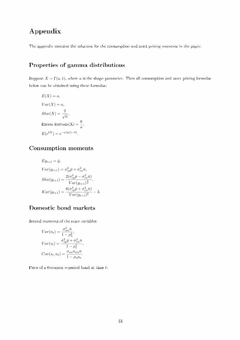
Appendix
The appendix contains the solutions for the consumption and asset pricing moments in the paper.
Properties of gamma distributions
Suppose X ∼ Γ(a, 1), where a is the shape parameter. Then all consumption and asset pricing formulas
below can be obtained using these formulas:
E(X) = a,
V ar(X) = a,
Skw(X) =2√a,
Excess kurtosis(X) =6
a,
E(ebX) = e−a ln(1−b).
Consumption moments
Egt+1 = g,
V ar(gt+1) = σ2cpp+ σ2
cnn,
Skw(gt+1) =2(σ3
cpp− σ3cnn)
V ar(gt+1)32
,
Kur(gt+1) =6(σ4
cpp+ σ4cnn)
V ar(gt+1)2− 3.
Domestic bond markets
Second moments of the state variables:
V ar(nt) =σ2nnn
1− ρ2n
,
V ar(st) =σ2spp+ σ2
snn
1− ρ2s
,
Cov(st, nt) =σsnσnnn
1− ρsρn.
Price of a 0-coupon n-period bond at time t:
43

Pn,t = eCn+Snst+Nnnt ,
Cn = Gn + Sns+ Pnp+ Nnn,
G1 = lnβ − γg,
S1 = −(γ − 1)(1− ρs),
P1 = −f(ap),
N1 = 0,
S1 = (γ − 1)(1− ρs),
N1 = −f(an),
Gn = lnβ − γg + Gn−1,
Sn = −(γ − 1)(1− ρs) + Sn−1 + Sn−1(1− ρs),
Pn = Pn−1 − f(ap + Sn−1σsp),
Nn = Nn−1 +Nn−1(1− ρn),
Sn = (γ − 1)(1− ρs) + ρsSn−1,
Nn = ρnNn−1 − f(an + Sn−1σsn +Nn−1σnn).
Variance of the one period risk-free rate:
V ar(y1) = (1− γ)2(1− ρs)2V ar(st) + f(an)2V ar(nt) + 2(1− γ)(1− ρs)f(an)Cov(st, nt).
Expectations hypothesis coe�cient from the regression yn−1,t+1 − yn,t = β0 + βn1
n−1 (yn,t − y1,t) + εt:
βn =Cov(Et(yn−1,t+1 − yn,t), yn,t − y1,t)
V ar(yn,t − y1,t)
= 1−(ρnNn−1 −Nn +N1)(− 1
nNn +N1)V ar(nt) + (ρnNn−1 −Nn +N1)(− 1nSn + S1)Cov(st, nt)
(− 1nSn + S1)2V ar(st) + (− 1
nNn +N1)2V ar(nt) + 2(− 1nSn + S1)(− 1
nNn +N1)Cov(st, nt).
International markets
Two countries are assumed to have the same parameters. The shocks are assumed to be uncorrelated
across two countries.
The uncovered interest rate coe�cient from the regression rFXt+1 = α0 + αFX(y1,t − y∗1,t) + εt:
αUIP =Cov(−y1,t + y∗1,t + Et(m
∗t+1 −mt+1), y1,t − y∗1,t)
V ar(y1,t − y∗1,t)
=−N2
1V ar(nt)− S1N1Cov(st, nt)
S21V ar(st) + (N2
1 )V ar(nt) + 2S1N1Cov(st, nt).
Variance of the changes in the real exchange rates:
V ar(∆et+1) = V ar(m∗t+1 −mt+1) = 2((1− γ)2(1− ρs)2V arst + a2pp+ a2
nn).
44

Correlation between the exchange rate changes and the consumption growth di�erentials:
Corr(∆et+1, g∗t+1 − gt+1) = Corr(m∗t+1 −mt+1, g
∗t+1 − gt+1) =
2(σcpapp− σcnann)√2V ar∆et+1V ar(gt+1)
.
Equity
Assuming, following Cambpell and Cochrane (1999) and Bekaert and Engstrom (2009), that dividends
equal consumption, the price-dividend ratio is:
Pt
Dt=
∞∑i=1
eCei +Se
i st+Nei nt ,
Cei = Ge
i + Sei s+ P e
i p+ Ne1 n,
Ge1 = lnβ + (1− γ)g,
Se1 = −(γ − 1)(1− ρs),
Ne1 = 0,
P e1 = −f(ap + σcp),
Se1 = (γ − 1)(1− ρs),
Ne1 = −f(an − σcn),
Gen = Ge
n−1 + lnβ + (1− γ)g,
Sen = Se
n−1 + Sen−1(1− ρs)− (γ − 1)(1− ρs),
P en = P e
n−1 − f(ap + σcp + Sen−1σsp),
Nen = Ne
n−1 +Nen−1(1− ρn),
Sen = (γ − 1)(1− ρs) + ρsSn−1,
Nen = Ne
n−1ρn − f(an − σcn + Sen−1σsn +Ne
n−1σnn).
Note that the expression above is non-linear in the state variables nt and qt, which is not very convenient
to compute the expected returns. The �rst order Taylor approximation of the logarithm of the price
dividend ratio around the steady state is:
pdt ≈ ln
∞∑i=1
eCei +Se
i s+Ne1 n +
∑∞i=1 e
Cei +Se
i s+Ne1 nSe
i∑∞i=1 e
Cei +Se
i s+Ne1 n
(st − s) +
∑∞i=1 e
Cei +Se
i s+Ne1 nNe
i∑∞i=1 e
Cei +Se
i s+Ne1 n
(nt − n)
≡ K1 +Ks1st +Kn
1 nt.
Similarly:
ln(1 +Pt
Dt) ≈ ln(1 +
∞∑i=1
eCei +Se
i s+Ne1 n) +
∑∞i=1 e
Cei +sei s+Ne
1 nSei
1 +∑∞
i=1 eCe
i +Sei s+Ne
1 n(st − s) +
∑∞i=1 e
Cei +Se
i s+Ne1 nNe
i
1 +∑∞
i=1 eCe
i +Sei s+Ne
1 n(nt − n)
≡ K2 +Ks2st +Kn
2 nt.
45

Using the linear approximations above, the equity premium is:
Et(rmkt,t+1 − y1, t) =Et(ln(1 +Pt+1
Dt+1)− ln
Pt
Dt+ gt+1 − y1,t)
≈K2 −K1 +Ks2(1− ρs)s+Kn
2 (1− ρn)n+ lnβ − (γ − 1)(1− ρs)s− f(ap)p+
(Ks2ρs −Ks
1 + (γ − 1)(1− ρs))st + (Kn2 ρn −Kn
1 − f(an))nt.
46

Figure 1: Unconditional Distribution of Consumption Growth in US and in the Model.
The data are annual. The US data is the logarithmized per capita total consumption
growth. The time period is 1929-2012. The model implied distribution is obtained by
sampling 100,000 annual observations from the model.
47
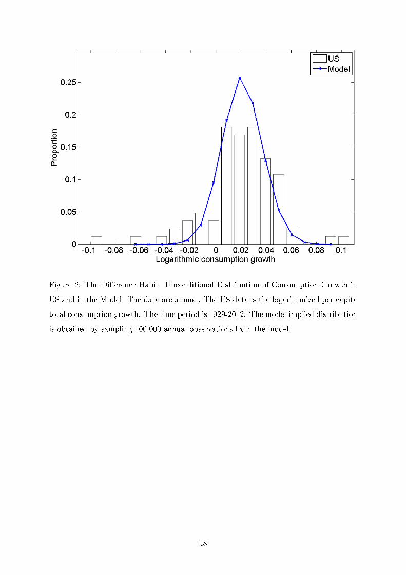
Figure 2: The Di�erence Habit: Unconditional Distribution of Consumption Growth in
US and in the Model. The data are annual. The US data is the logarithmized per capita
total consumption growth. The time period is 1929-2012. The model implied distribution
is obtained by sampling 100,000 annual observations from the model.
48
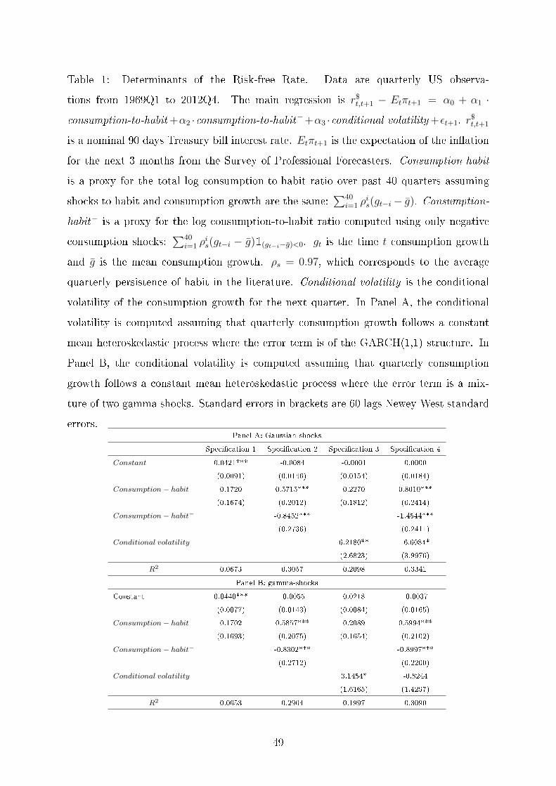
Table 1: Determinants of the Risk-free Rate. Data are quarterly US observa-
tions from 1969Q1 to 2012Q4. The main regression is r$t,t+1 − Etπt+1 = α0 + α1 ·
consumption-to-habit +α2 ·consumption-to-habit−+α3 ·conditional volatility +εt+1. r$t,t+1
is a nominal 90 days Treasury bill interest rate. Etπt+1 is the expectation of the in�ation
for the next 3 months from the Survey of Professional Forecasters. Consumption-habit
is a proxy for the total log consumption-to-habit ratio over past 40 quarters assuming
shocks to habit and consumption growth are the same:∑40
i=1 ρis(gt−i− g). Consumption-
habit− is a proxy for the log consumption-to-habit ratio computed using only negative
consumption shocks:∑40
i=1 ρis(gt−i − g)1(gt−i−g)<0. gt is the time t consumption growth
and g is the mean consumption growth. ρs = 0.97, which corresponds to the average
quarterly persistence of habit in the literature. Conditional volatility is the conditional
volatility of the consumption growth for the next quarter. In Panel A, the conditional
volatility is computed assuming that quarterly consumption growth follows a constant
mean heteroskedastic process where the error term is of the GARCH(1,1) structure. In
Panel B, the conditional volatility is computed assuming that quarterly consumption
growth follows a constant mean heteroskedastic process where the error term is a mix-
ture of two gamma shocks. Standard errors in brackets are 60 lags Newey-West standard
errors.Panel A: Gaussian shocks
Speci�cation 1 Speci�cation 2 Speci�cation 3 Speci�cation 4
Constant 0.0421*** -0.0084 -0.0001 0.0000
(0.0091) (0.0146) (0.0154) (0.0184)
Consumption− habit 0.1720 0.5715*** 0.2270 0.8010***
(0.1674) (0.2012) (0.1812) (0.2414)
Consumption− habit− -0.8452*** -1.4544***
(0.2736) (0.2411)
Conditional volatility 6.2180** -6.6084*
(2.6823) (3.9976)
R2 0.0673 0.3057 0.2098 0.3341
Panel B: gamma-shocks
Constant 0.0440*** -0.0055 0.0218 -0.0037
(0.0077) (0.0143) (0.0084) (0.0165)
Consumption− habit 0.1702 0.5857*** 0.2089 0.5994***
(0.1693) (0.2075) (0.1654) (0.2102)
Consumption− habit− -0.8302*** -0.8997***
(0.2712) (0.2200)
Conditional volatility 3.1454* -0.8244
(1.6165) (1.4297)
R2 0.0653 0.2964 0.1997 0.3090
49

Table 2: Aggregate Per Capita Consumption Growth Volatilities for G10 Carry Trade
Countries. Data is annual. Portfolio consumption growths are GDP weighted consump-
tion growths of portfolio countries. In Panel A, Volatilities are computed from the time
series of consumption growths. Bootstrap standard errors are in brackets. In Panel B,
in each bootstrap run a time series of the historical length is sampled for each portfolio,
preserving the time relationship between the time series (that is if the observation for
1996 is sampled for the high-interest rate portfolio it is also sampled for the mid- and
low-interest rate portfolios). Then, volatilities of these time series are computed. p-value
is the proportion of bootstrap runs where the volatility of a row time series is larger
than the volatility of a column time series. 10,000 bootstrap runs are performed for both
Panels A and B. The asterisks, *, **, and ***, correspond to the statistical signi�cance
at 10, 5, and 1 percent levels, respectively.Panel A: Historical consumption growth volatilities
Low-interest rate countries Mid-interest rate countries High-interest rate countries
Japan, Switzerland Canada, Germany, Sweden, UK, US Australia, New Zealand, Norway
Whole time period: 1971-2012
1.94% 1.42% 1.18%
(0.22%) (0.14%) (0.13%)
Modern time period: 1988-2012
1.42% 1.24% 1.21%
(0.22%) (0.21%) (0.22%)
Panel B: Bootstrap p-values for the di�erences in historical consumption growth volatilities
Whole time period: 1971-2012
Low-interest rate countries Mid-interest rate countries High-interest rate countries
Low-interest rate countries - 0.9867** 0.9976***
Mid-interest rate countries 0.0133** - 0.8881
High-interest rate countries 0.0024*** 0.1119 -
Modern time period: 1988-2012
Low-interest rate countries Mid-interest rate countries High-interest rate countries
Low-interest rate countries - 0.8217 0.7960
Mid-interest rate countries 0.1783 - 0.5387
High-interest rate countries 0.2040 0.4613 -
50

Table 3: Parameters of the Model. Preferences and consumption dynamics parameters for the baseline
speci�cation of the model. The parameters are calibrated to match the basic consumption and asset
pricing dynamics. The parameters are for the annual calibration frequency. The implied local relative
risk-aversion, de�ned as γeqt approximately corresponds to the CRRA-utility risk-aversion. The distri-
bution of the implied local relative risk-aversion is computed by sampling 100,000 annual observations
from the model.
Parameter Interpretation Value
Preferences
β discount factor 0.9750
γ risk-aversion 6.6865
s average consumption-habit ratio 1.0000
ρs persistence of the consumption-habit ratio 0.7860
σsp sensitivity of the consumption-habit ratio to positive shocks 0.0001
σsn sensitivity of the consumption-habit ratio to negative shocks -0.1604
Consumption dynamics
g average consumption growth 0.0210
p shape parameter of positive shocks 202.2554
σcp impact of the positive shocks on the consumption growth 0.0017
n average shape parameter of negative shocks 0.0185
σcn impact of the negative consumption shocks on the consumption growth 0.0519
ρn volatility persistence 0.8758
σnn scale of the volatility shock 0.0770
51

Table 4: Per Capita Consumption Growth Dynamics in The Model and Data. The US
data is the logarithmized annual per capita total consumption growth. The time period
is 1929-2012. The model statistics for disaster probabilities is computed by sampling
100,000 annual observations from the model. g and σg are unconditional mean and
standard deviation of the consumption growth, respectively.
Mean Standard deviation Skewness Excess kurtosis P (< g − 2σg) P (< g − 4σg)
Model 2.10% 2.52% -0.20 2.02 1.93% 0.11%
US 2.00% 2.98% -0.83 3.52 4.96% 1.20%
52

Table 5: Asset Pricing Moments. All moments are annual moments. For the international
statistics, it is assumed that two countries have exactly the same model parameters as
reported in Table 3, and shocks are independent across two countries. All model generated
moments are in real terms. All data moments are in real terms except the expectation
hypothesis coe�cients and the uncovered interest rate parity coe�cients. Real yields data
are US 2004-2012 data. Expectation hypothesis data are US 1961-2012 data. Equity data
are US 1926-2012 data. The uncovered interest rate parity coe�cient is the average UIP
coe�cient for the US dollar and most common foreign currencies from Backus et.al.
(2001). The correlation between the consumption growth rates di�erentials and the real
exchange rate changes are from Benigno and Thoenissen (2008). The volatility of the
real exchange rate changes is from Croce and Colacito (2011).Moment Description Model Data
Real zero-coupon yields
y1 1 year 0.20% 0.23%
y2 2 years 0.48% 0.37%
y3 3 years 0.75% 0.49%
y4 4 years 1.01% 0.63%
y5 5 years 1.26% 0.78%
σ(y1) volatility of the 1 year yield 1.65% 1.58%
Expectation hypothesis coe�cients from the regression yn−1,t+1 − yn,t = β0 + βn1
n−1(yn,t − y1,t) + εt
β2 n=2 years -1.18 -0.71
β3 n=3 years -1.21 -1.04
β4 n=4 years -1.27 -1.29
β5 n=5 years -1.31 -1.48
Equity
rmkt − y1 equity premium 4.45% 5.67%
Sharpe-ratio 0.36 0.29
pd logarithm of the price-dividend ratio 3.66 3.40
Corr(pdt−1, pdt) autocorrelation of the price-dividend ratio 0.81 0.85
International
αFX from regression rFXt+1 = α0 + αFX(y1,t − y∗1,t) + εt -1.92 [-0.74,-1.84]
σ(∆et+1) volatility of the real exchange rate 20.12%20 11.21%
Corr(∆et+1, g∗t+1 − gt+1) correlation between the exchange rate changes and the
consumption growth di�erentials
-0.49 [-0.55,0.53]
2020.12% is for the case of uncorrelated consumption growth shocks across two countries. For the case
where the correlation between consumption growth shocks in two countries is 0.32, which corresponds
to the correlation between US and UK consumption growths, the exchange rate volatility is 16.46%.
53

Table 6: Alternative Model Calibration: Downward Sloping Yield Curve And "Non-
violated" Expectation Hypothesis. All moments are annual real moments. g and σg
are unconditional mean and standard deviation of the consumption growth, respectively.
yn is the yield for a horizon n risk-free zero-coupon bond. βn is the coe�cient from the
yn−1,t+1−yn,t = β0 +βn1
n−1(yn,t−y1,t)+εt regression. rmkt−y1 is the equity risk-premium.
pd is the natural logarithm of the price-dividend ratio.PANEL A: PARAMETERES
β γ s ρs σsp σsn
0.9700 14.9134 1.0000 0.8464 0.0001 -0.0449
Consumption dynamics
g p σcp n σcn ρn σnn
0.0210 119.5582 0.0023 0.1018 0.0420 0.6669 0.2755
PANEL B: CONSUMPTION AND ASSET PRICING MOMENTS
Consumption growth
Mean Standard deviation Skewness Excess kurtosis P (< g − 2σg) P (< g − 4σg)
2.10% 2.84% 2.97. -0.53 2.26% 0.27%
Real yields
y1 y2 y3 y4 y5 σ(y1)
0.68% 0.43% 0.26% 0.18% 0.17% 2.40%
Expectation hypothesis coe�cients
β2 β3 β4 β5
2.55 2.27 1.91 1.45
Equity
rmkt − y1 Sharpe-ratio pd Corr(pdt−1, pdt)
4.08% 0.23 3.62 0.86
54

Table 7: The Di�erence Habit Calibration. All moments are annual real moments. g and
σg are unconditional mean and standard deviation of the consumption growth, respec-
tively. yn is the yield for a horizon n risk-free zero-coupon bond. βn is the coe�cient
from the yn−1,t+1 − yn,t = β0 + βn1
n−1(yn,t − y1,t) + εt regression. αFX is the coe�cient
from the rFXt+1 = α0 +αFX(y1,t− y∗1,t) + εt regression. rmkt− y1 is the equity risk-premium.
pd is the natural logarithm of the price-dividend ratio.PANEL A: PARAMETERES
β γ q ρq σqp σqn
0.9964 3.6740 1.0000 0.8049 -0.0002 0.1956
Consumption dynamics
g p σcp n σcn ρn σnn
0.0210 197.4329 0.0011 0.1095 0.0114 0.8581 0.1878
Implied local relative risk-aversion
Mean Median 90th-percentile 95th-percentile 99th-percentile
10.0522 9.6007 10.9753 12.1335 16.1032
PANEL B: CONSUMPTION AND ASSET PRICING MOMENTS
Consumption growth
Mean Standard deviation Skewness Excess kurtosis P (< g − 2σg) P (< g − 4σg)
2.10% 1.62% 0.06 0.19 2.05% 0.02%
Real yields
y1 y2 y3 y4 y5 σ(y1)
0.55% 0.78% 1.00% 1.21% 1.40% 1.41%
Expectation hypothesis coe�cients
β2 β3 β4 β5
-0.87 -0.88 -0.90 -0.94
Equity
rmkt − y1 Sharpe-ratio pd Corr(pdt−1, pdt)
5.53% 0.37 3.21 0.80
International
αFX σ(∆et+1) Corr(∆et+1, g∗t+1 − gt+1)
-1.56 38.50%21 -0.46
2138.50% is for the case of uncorrelated consumption growth shocks across two countries. For the case
where the correlation between consumption growth shocks in two countries is 0.32, which corresponds
to the correlation between US and UK consumption growths, the exchange rate volatility is 31.75%.
55

Table 8: Comparision to Other Models. All values are at annual frequency unless men-
tioned otherwise. Samples, and thus calibration objectives, are slightly di�erent across
the studies. These di�erences do not a�ect qualitative implications of the models (e.g.,
does the expectation hold or not). µ is the average consumption growth. σ is the standard
deviation of the consumption growth. y5 and y1 are 1 and 5 years yields, respectively.
β2 is the regression coe�cient from the y1,t+1 − y1,t = β0 + β2(y2,t − y1,t) + εt regres-
sion run with annual data. UIP coe�cient is the αFX coe�cient from the regression
rFXt+1 = α0 + αFX(y1,t − y∗1,t) + εt. A colored cell points out an inconsistency between the
model and the data.This
paper
Habit:
Wachter
(2002)
Habit:
Verdelhan
(2010)
Long-run risk: Bansal
and Shaliastovich
(2013)
Rare disasters:
Gabaix, 2012
Data: US
Risk-aversion 6.69 ≈ 30 ≈ 30 20.90 4 < 101
Disaster probability (gt < µ− 4σ) 0.11% 0.00% 0.00% 0.03% 3.63% 1.20%
Real yield curve slope, y5 − y1 1.06% 0.89% -0.46% <0.00% 0.00% 0.55%
Expectation hypothesis: β2 -1.18 −0.972 >0.00 −0.452,3 −1.922,3 −0.713
UIP coe�cient -1.92 >0.00 -1.99 −2.063 <-1.00 −2.294
1 - based on the literature review in Mehra and Prescott (1985)
2 - the short-term bond is a 3 month treasury bill
3 - nominal value
4 - for the US-UK pair
56


