

2017
NAU STUDENT
NORTHERN ARIZONA UNIVERSITY | Mechanical Engineering Department
Abdulaziz Alanzi
Abdullateef Alhumaidan
Galen Geislinger
Thomas Hill
Brianna Moore
Clayton Surratt
1 | Page
Abdulaziz Alanzi
Abdullatif Alhumaidan
Galen Geislinger
Thomas Hill
Brianna Moore
Clayton Surratt
2016-17
Project Sponsor: Salt River Project
Faculty Advisor: Dr. David Trevas
Sponsor Mentor: Vy Kieu
Instructor: Dr. David Trevas
SRP FLUIDS ANALYSIS
Midpoint Report

2 | Page
DISCLAIMER
This report was prepared by students as part of a university course requirement. While
considerable effort has been put into the project, it is not the work of licensed engineers and
has not undergone the extensive verification that is common in the profession. The
information, data, conclusions, and content of this report should not be relied on or utilized
without thorough, independent testing and verification. University faculty members may
have been associated with this project as advisors, sponsors, or course instructors, but as such
they are not responsible for the accuracy of results or conclusions.

3 | Page
ACKNOWLEDGEMENTS
We thank Dr. David Trevas our faculty advisor for his time and effort, and for sharing his
solutions and ideas with us as a team. We also thank Salt River Project for giving us this
opportunity. We are also thankful for Vy Kieu’s assistance in providing us with the
appropriate data needed to successfully find a solution. We also would like to thank Dr. Tom
Acker for providing us many useful resources from his books and knowledge.

4 | Page
Table of Contents
DISCLAIMER i
ACKNOWLEDGEMENTS ii
1 6
1.1 6
1.2 6
1.3 6
1.3.1 6
1.3.2 7
1.3.3 7
1.3.4 7
2 8
2.1 8
2.2 8
2.3 9
2.4 9
2.5 10
3 12
3.1 12
3.2 12
3.2.1 12
3.2.2 13
3.2.3 13
3.3 13
3.3.1 14
3.3.1.1 14
3.3.1.2 15
3.3.1.3 15
3.3.2 15
3.3.2.1 15
3.3.2.2 15
3.3.2.3 16
3.3.3 16
3.3.3.1 16
3.3.3.2 16
3.3.3.3 16

5 | Page
4 17
4.1 17
4.2 17
4.3 18
4.4 18
4.5 19
4.6 20
4.7 20
4.8 21
4.9 21
4.10 22
5 23
5.1 23
5.2 25
5.2.1 25
5.2.2 27
6 28
7 30
7.1 30
7.1.1 30
7.2 31
7.2.1 31
7.2.2 31
7.2.3 31
7.2.4 33
7.2.5 35
7.2.6 37
7.2.7 39
7.2.8 40
References 29
Appendix A 31

6 | Page
1 BACKGROUND
1.1 Introduction
This project is sponsored by Salt River Project (SRP) located in Phoenix, AZ who supplies
power to one million customers in the Phoenix area. SRP has 12 power plants which use a
fuel measurement system that was evaluated for redesign. The goal was to improve the fuel
measurement in both fuel measurement accuracy and to improve the process efficiency of
SRP’s natural-gas-fired power plants. This project interests SRP because they want their
plants to be at the maximum possible efficiency and fuel measurement accuracy so that they
may continue serving their 1 million customers. These results would benefit Phoenix as a
whole because increased efficiency at SRP’s natural gas-fired power plants would result in
less waste, saving the consumer money. A more efficient natural-gas process will not only
benefit SRP but is important to finding a solution to the energy crisis, especially as natural gas
is an increasingly common and cheap energy source.
1.2 Project Description
Following is the original project description given to the SRP Fluids Analysis group from SRP.
“The project goal will be to improve fuel measurement accuracy and process efficiency
at each of SRP’s natural-gas power plants. In order to succeed, the project team will
collaborate with engineers, operators, and instrument technicians at several SRP power
plants. Project scope includes assessment of fuel delivery systems, fuel measurement
devices, fuel flow calculations, power plant operations, and multi-department process
coordination.”
1.3 Original System
Figure 1.3: Original System Diagram
1.3.1 Original System Structure
SRP buys their natural gas from the company Kinder Morgan, the largest energy infrastructure
company in North America. The Orifice Plate is a device used to measure flow rate and restrict
7 | Page
pressure or flow rate. The Rosemount and Flo Boss are both connected to the Orifice Plate and
both pick up pressures and flow rates. The difference between the two is that the Flo Boss can
also read temperatures.
1.3.2 Original System Operation
SRP first receives their natural gas from Kinder Morgan which is then pumped into SRP’s fuel
measurement system. The gas passes through the orifice plate that measures the gas and sends
the readings to the Rosemount transmitter and the Flo Boss which is more of a redundancy for
the gas readings. The gas continues past the Orifice Plate and goes into the system where it's
put through a process where the temperature is 1000 F making steam. The steam is then put
through steam turbines and converted into energy.
1.3.3 Original System Performance
SRP has sent the team a few files that have helped with coming up with reasonable redesign
ideas and concept generations. SRP provided us with all metering information going from gas
composition, differential pressure, to the temperature inside the pipe. SRP also sent the team
gas prices and some receipts from Kinder Morgan compared to their metering which shows
difference in measurements, which one of your members will be doing an analytical analysis
on.
1.3.4 Original System Deficiencies
One main reason SRP needs to redesign their fuel measurement system is because of a 2% error
margin. Kinder Morgan supplies SRP with natural gas. Both companies make gas
measurements on their portions of the gas transport system, with their measurements differing
by 2%. The project goal was to minimize this 2% error while staying within the allotted budget.
8 | Page
2 REQUIREMENTS
The following customer requirements define the project’s priorities and identify which goals
may conflict with each other. They consider economic, technical, regulatory, and political
aspects of the project, offering a more complete and realistic design. Each requirement is
weighted to show its importance, which will be useful when making decisions about conflicting
goals.
2.1 Customer Requirements (CRs)
The team has created 11 Customer Requirements for this project. The design:
1. Will uphold the standards and comply with the regulations of SRP, with a special
consideration for safety. Weighting: 10
2. Must increase the accuracy of the fuel measurement system, either by updating or
replacing the current system. Weighting: 10
3. Includes redundancies so that if one part of the design fails, the entire system will
continue running, as plant shut downs are extremely expensive to the company.
Weighting: 9
4. Be completed under a budget of $3000, as allotted by SRP. Weighting:10
5. Not increase greenhouse gas emissions, to avoid contributing to global warming and
adhere to governmental emission regulations. Weighting: 6
6. Be easily adoptable by current operators and easy to use. Weighting: 7
7. Will monitor gas composition in real time, so that leaks or changes in composition can
be known. Weighting: 8
8. Adapt to maintain maximum accuracy and efficiency as the plan powers on and off and
changes power input. Weighting: 9
9. Will be adaptable to each SRP natural-gas power plant so that the design may be as
useful as possible. Weighting: 8
10. Will be reliable, as even small differences in measurements may negatively affect the
error margin. Weighting: 8
11. Will meet any applicable EPA regulations. Weighting: 10
2.2 Engineering Requirements (ERs)
The previously listed Customer Requirements were then considered to create more
technically specific Engineering Requirements. The design will:
1. Decrease the error in gas measurement to less than 0.5%, ideally to 0.25%.
2. Cost less than the allotted budget of $3000, though the more cost-effective, the better.
3. Withstand measuring between 1,000 and 10,000 mcf/day, which is a measurement
difference factor of 10.
4. Be able to withstand up to 100 psig of pressure.
5. Include a weather-resistant computer (or one in a weatherproof box), as the design
will be exposed to the elements.
6. Include a flowmeter made of a non-corrosive material.
7. Be compatible with the existing pipe structures, which have diameters of 6 in, 14 in,
and 16 in.
8. Include a real-time data display, such as an LCD screen or dial, so the operators may
make measurements in the field.
9. Meet SRP and EPA safety regulations.
10. Last at least 15 years, with a design goal of 20 years.
9 | Page
11. Include at least 1 redundancy for every function. This may include leaving some of
the existing meters in place, as the company has done with the Rosemont system.
12. Reduce the pressure drop, which is currently 0.02 psi, in order to reduce turbulence.
2.3 Testing Procedures (TPs)
1. The fluid dynamics for each type of meter are to be tested using computer modeling.
First, the team developed MATLAB code to help with more simple math, and then a
model of each meter was tested using numerical analysis techniques, showing
potential losses in energy, laminar and turbulent flows, and overall which meters will
perform the best.
2. The team can test various meters in Northern Arizona University’s thermofluids
lab. This can be done by setting up a loop with a fluid, whose properties can be
easily determined or measured, air would be a common fluid to use. This loop of
chosen fluid then can be directed through various meters of the team’s choosing and
pressure differences can be measured with pressure taps and a data acquisition
device. This data will allow the team to determine the amount of pressure drop for
each meter and infer which meter would be best for the application.
3. Economic analysis
4. Because the meter was purchased from a manufacturer instead of fabricated by the
team, manufacturer’s specs was used to evaluate whether certain engineering
requirements have been met, such as life expectancy.
2.4 Design Links (DLs)
1. In order to comply with the engineering requirement where the gas measurement has
to be less than 0.5%, the team suggested the idea where as long as the design has a
very low pressure drop, lower than the existing design, it will satisfy this requirement.
2. The team’s design is considered to be a bit off the budget, where the estimated price
is $4000 and our allotted budget is $3000. However, our allotted budget could be
flexible and might be able to cover the cost.
3. According to the analytical analysis made on the Venturi flowmeter, the team
obtained a turndown ratio less than ten, which satisfies this criterion in particular.
Also, the Venturi flowmeter withstands measurements between 1000 and 10000
mcf/day.
4. The team planned to use AISI 1020 steel as the material for the design. The AISI
1020 steel has a tensile strength more than 5000 psi. Therefore, the material
withstands pressure that exceeds 100 psig. It is also considered to be a non-corrosive
material, and meets the required 15 year design life.
5. See number 4
6. The manufacturer who is supplying the Venturi meters for our team has the option to
change the diameter of the flowmeter to anything necessary. So, it was easy to
purchase meters of the correct diameter to be compatible with the pipe.
7. After inspecting EPA and discussing with SRP their safety regulations. The team can
safely say that the final design meets SRP and EPA safety regulations.
8. See number 4
9. There are three units that need to be fitted with flowmeters. So, in order to create a
redundancy the team can purchase a total of four flowmeters for the units. Purchasing
the extra flowmeter will make it so that in the event of a failure the extra flowmeter
can be installed instead of fixing the broken one.
10 | Page
10. To reduce the pressure drop experienced by the existing orifice plate, the team
implemented a Venturi tube meter, which due to the geometry of the venturi tube,
will create less of a pressure drop. This is due to the converging and diverging
sections of the pipe keeping the total head of the fluid constant throughout the meter.
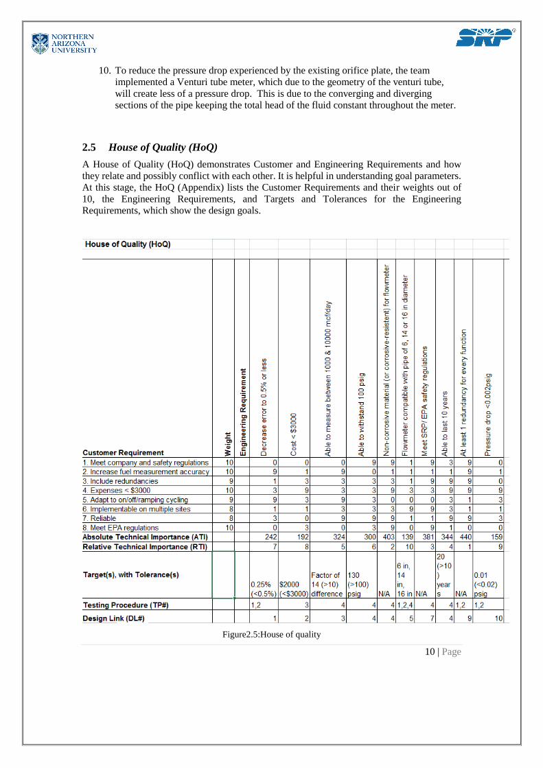
2.5 House of Quality (HoQ)
A House of Quality (HoQ) demonstrates Customer and Engineering Requirements and how
they relate and possibly conflict with each other. It is helpful in understanding goal parameters.
At this stage, the HoQ (Appendix) lists the Customer Requirements and their weights out of
10, the Engineering Requirements, and Targets and Tolerances for the Engineering
Requirements, which show the design goals.
Figure2.5:House of quality

11 | Page

12 | Page
3 EXISTING DESIGNS
The following information regards existing designs that are currently in use for the entire
process of converting natural gas into useable energy. This section will elaborate on current
industry practices and the team’s rationale as to why these industry practices are relevant to
our design process.
3.1 Design Research
In order to get an accurate idea of what the usual practices and industry standards are for natural
gas plants the group conducted extensive research into contemporary natural gas systems and
subsystems. For system level design the areas that were focused on were the measurement of
the natural gas and the general thermodynamic processes that take place for converting natural
gas into useable energy. For subsystems the areas that were researched were specific
measurement techniques, transportation methods, and turbine designs used in natural gas plants.
The main source of information gathered during our design research was published research
and informative articles found via the internet. Specific calculations were difficult to find via
open source online information due to the fact that this sort of information is proprietary to each
respective natural gas company. However, online research was extremely valuable for
obtaining system overviews and rationale as to why certain design decisions are made by
natural gas distributors and energy generation companies. Specific information regarding the
specifications of our design will be supplied by our client contact at SRP and will be included
in subsequent reports.
3.2 System Level
One of the preliminary steps in designing or improving a system is to find out what the standard
practices are for similar systems. With this in mind two areas were focused on in the research
of existing systems, they were methods of natural gas measurement and methods of converting
natural gas into useable energy.
Included in existing designs is an example of a state of the art natural-gas measurement system
being used in Turkey and two examples of the two most common methods of natural-gas
combustion. These three existing designs were selected because both measurement and energy
generation techniques are extremely pertinent to our design process going forward.
3.2.1 Existing Design #1: Turnkey Gas Measurement System
One of the existing systems that was researched was the Turnkey Gas Measurement System
designed by Botas, which is the state owned oil and gas company in Turkey. The system was
designed to compress natural gas to 75 bar at flow rates that vary between 510,000 and
2,040,000 Sm3 per hour [1]. This pressure and flow rate need to be maintained during all
seasons, which can be a challenge in a country with a volatile climate, like Turkey.
A few of the elements of the Botas systems that differ from similar systems designed by
different companies are that the Botas system has all components designed together as a
package, instead of separate, and the Botas system has numerous intended redundancies
incorporated into it [1]. The benefits of having all of the components designed as one package
are that cost is significantly reduced, and the chance of components not integrating with each
other successfully is significantly mitigated. The purpose of the redundancies in the system is
to attempt to eliminate the risk of one component malfunction causing the system to shut down.
In the energy industry downtime can be extremely expensive, so it was determined that it would
13 | Page
be more cost effective to allocate more resources to creating redundancies in the design and
reduce the chance of the entire system needing to be shut down for maintenance.
3.2.2 Existing Design #2: Simple Cycle Power Plant
One of the existing types of natural gas energy generation systems is the simple cycle natural
gas power plant. This system works by performing a basic cycle where natural gas is combusted
which causes the gas to expand and rotate a series of blades attached to the shaft. This causes
the shaft to turn and spin a generator which produces electricity. One of the issues with simple
gas turbines is that the process efficiency is only 20-35% [2]. The benefit of a simple cycle over
the other types of cycles is that a simple cycle is much less expensive to initially design and
build. This makes it so that for areas where a small amount of energy is need a simple power
cycle will make more sense. For areas where a large amount of energy is needed it makes more
sense to invest in a more efficient system
3.2.3 Existing Design #3: Combined-Cycle Power Plant
One of the existing systems researched is the combined-cycle power plant. This plant uses gas
and steam turbines that produce up to 50 percent more electricity, using the same amount of
fuel than the traditional simple-cycle plant [3]. Any heat waste from the system is also rerouted
to the steam turbine, and generates more power.
This system works by first the gas turbines burn the fuel put into the system. The gas turbine
compresses the air and mixes it with fuel at a high temperature. The heated air moves through
the turbine blades making them spin. The fast spinning blades drives the generator that converts
some of the energy into useful electrical power. The combined-cycle plant also has a heat
recovery system that captures exhaust [3]. A heat recovery system generator (HRSG) captures
exhaust heat from the gas turbine, that would’ve have escaped and been wasted. Then the HRSG
takes the heat and sends it to the steam turbine. The steam turbine then takes the excess exhaust
waste and makes it into useful electrical power.
3.3 Subsystem Level
Throughout our research of existing system level designs it became apparent that there are three
subsystem levels that are the most important to the process of converting natural gas into
useable energy. The functional model (Figure 3.1) in the figure below describes the measured
flow at SRP’s Agua Fria plant. Kinder Morgan sends its fluid to SRP’s pipeline to be measured
through an orifice plate that is being calculated by a flow computer, the FloBoss. The rest of
system is how energy is transformed from mechanical energy to electricity. These subsystems
are: measurement of incoming natural gas, transportation of that natural gas, and the different
kinds of turbines used to convert combusted gas into energy. In the following sections the
importance of these three subsystems and the specific methods used in these subsystems is
explained in detail.

14 | Page
Figure 3.1: Functional model of the natural gas system at the Agua Fria plant
3.3.1 Subsystem #1: Measurement
The general idea of measurement on this subsystem is coming from adsorption operation. There
are commonly used sorbents like zeolites or activated carbons. The method and designs to
calculate the mass of a gas are various, but the three existing designs that will be discussed here
are the Volumetric, Gravimetric, and the Oscillometric chromatographic methods.
3.3.1.1 Existing Design #1: Volumetric – chromatographic
The system shown is a slow processed system, because of the fact that the mixture will go
through many steps to be adsorbed, but it still can give accurate measurements not just for
natural gas, but also for other gasses. The way it works is by supplying a gas mixture to the
storage vessel that has a certain volume and measurement for pressure and temperature [4]. The
mixture from there will expand to the adsorption chamber, where it has an adsorbent that will
absorb gas. The chamber also has a certain volume and measurement for pressure and
temperature, which will allow a specific amount of mass for the rest of the mixture, enabling
the amount of absorbed gas to be calculated. The rest of the mixture however will circulate
back to the vessel storage by a circulation pump to do the process over and over again. The gas
sample will provide the mass concentration, which will eventually derive an equation for the
absorbed gas [4].

15 | Page
3.3.1.2 Existing Design #2: Gravimetric – chromatographic
For the gravimetric method a microbalance is placed inside the adsorption chamber instead of
two storages as the previous existing design. What this microbalance does is it will deal with
weighing the mixture before and after the adsorption operation to have accurate value for the
mixture and the gas. The molar mass will be needed as well and it will be calculated as before
by taking a gas sample. The process can also be repeated over and over again by a circulation
pump [4].
3.3.1.3 Existing Design #3: Oscillometric-Chromatographic
The Oscillometric chromatographic design can calculate the mass by the frequency of
oscillations of the sorbent. The number of frequency measured throughout the rotational
pendulum can give specific measurement of mass from the Reynold’s number equation. A
formula can be derived through experiments to calculate the mass adsorbed accurately [4].
3.3.2 Subsystem #2: Transportation
The transportation process of the natural gas is the most important aspect of the gas business,
where usually the gas plants are not located near the main markets. In general, natural gas can
be transported by pipelines, which is the method that the team will be working with during this
project. The transportation of natural gas through pipelines is considered to be very complicated
[5]. The pipeline network is very complex and needs to be designed to satisfy the supplier’s
route desire.
One way to ensure a less turbulent flow of the natural gas through pipelines is to pressurize the
gas that is being transported through the pipe. Pressurizing the gas will guarantee to deliver the
gas within the range of the desired rates and volumes. In addition, to ensure that the gas always
pressurized throughout its transportation, compressor stations are required to compress the
natural gas periodically, and this is done by placing compressor stations every 40 to 100 miles
[5]. The team is required to measure the natural gas at a constant rate. So, ensuring a constant
flow through the pipe will increase the accuracy of the measurements that will be done. Three
types of compression engines will be discussed more in depth below.
3.3.2.1 Existing Design #1: Centrifugal Compressor
The Centrifugal Compressor is a mechanical device mainly used for transporting purposes. The
Centrifugal Compressor moves the natural gas within the pipeline, which in a way increases
the flow speed of the gas because of the impellers that are included. In addition, the rotating
blades will increase the pressure of the natural gas that is transported. They are known to change
the direction of the gas flow by accelerating the gas flow within.
3.3.2.2 Existing Design #2: Reciprocating Engine
Also called a piston engine, this type of engine aims to generate rotational energy from pressure.
The reciprocating engine includes reciprocating pistons that play an essential role in converting
the pressure into rotational energy and moves the gas inside the pipe [6]. The reciprocating
engine uses the natural gas that is flowing inside the pipe to operate constantly. This engine
actually works by expanding the gas at a higher temperature and uses that work to operate the
pistons.
16 | Page
3.3.2.3 Existing Design #3: Hot Air Engine
The Hot air engine is a form of compressing gas within the pipeline to help accelerate and
move the natural gas to the desired location [7]. The Hot air engine takes advantage of the
expansion and contraction of the gas inside the pipe, which are caused by the thermal
differentiations, to convert thermal energy to mechanical energy. Based on that, it compresses
the gas and pumps it through the pipeline.
3.3.3 Subsystem #3: Flow measurement
During the process of natural gas transportation an accurate measurement of the flow rate is
needed in order to supply the correct amount of fuel into the combustion chamber that powers
the power plant. In order to get this measurement a multitude of flow measurement techniques
are used. A common technique so to to create a pressure drop in the flow and measure properties
across the pressure drop. Outside of this technique many others are used that do not have as
much impact on the flow of the fluid. In this section these techniques will be discussed in more
detail.
3.3.3.1 Existing Design #1: Sonic Flowmeter
A unique technique for measuring flow is with the use of a sonic flowmeter. The way this
works is that a device is attached to the flow area that sends a pulse perpendicular through the
flow. Once this pulse travels through the flow it is reflected back the way it came through the
flow. Once this has made the trip through the flow again the pulse is absorbed by a
transceiver. The transceiver records the time it took for the pulse to travel through the flow
and from that time the flow rate can be calculated.
3.3.3.2 Existing Design #2: Venturi Tube
A Venturi tube is a flow meter that has a contraction in the pipe making the diameter smaller
then getting larger again gradually to make the transition smooth and create less turbulence than
an orifice plate. This contraction makes a pressure difference much like the orifice plate where
the differential pressure is a key element in finding flow rate. To calculate this pressure
difference a manometer is attached to different sections on the Venturi tube, preferably before
and at the contraction.
3.3.3.3 Existing Design #3: Coriolis Meter
Over the past five years the Coriolis meter has been one of the fastest growing meter in the
market. Just like most meters Coriolis can calculate the mass flow rate of the fluid flowing
through it. Most Coriolis meters have two tubes which are made to vibrate in opposite
directions of each other due to the magnetic coil. Sensors in the form of magnet and coil
assemblies are mounted on the inlet and the outlet of both flow tubes. As the coils move
through the magnetic field created by the magnet, they create a voltage in the form of a sine
wave. These sine waves are then used to calculate the mass flow rate.
17 | Page
4 DESIGNS CONSIDERED
The following designs were the 10 most plausible designs resulting from the team’s
brainstorming. They include types of flowmeters, changes to the existing computer system
and orifice plate setup.
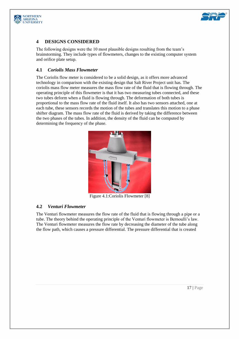
4.1 Coriolis Mass Flowmeter
The Coriolis flow meter is considered to be a solid design, as it offers more advanced
technology in comparison with the existing design that Salt River Project unit has. The
coriolis mass flow meter measures the mass flow rate of the fluid that is flowing through. The
operating principle of this flowmeter is that it has two measuring tubes connected, and these
two tubes deform when a fluid is flowing through. The deformation of both tubes is
proportional to the mass flow rate of the fluid itself. It also has two sensors attached, one at
each tube, these sensors records the motion of the tubes and translates this motion to a phase
shifter diagram. The mass flow rate of the fluid is derived by taking the difference between
the two phases of the tubes. In addition, the density of the fluid can be computed by
determining the frequency of the phase.
Figure 4.1:Coriolis Flowmeter [8]
4.2 Venturi Flowmeter
The Venturi flowmeter measures the flow rate of the fluid that is flowing through a pipe or a
tube. The theory behind the operating principle of the Venturi flowmeter is Bernoulli’s law.
The Venturi flowmeter measures the flow rate by decreasing the diameter of the tube along
the flow path, which causes a pressure differential. The pressure differential that is created

18 | Page
helps compute the flow rate.
Figure 4.2:Venturi Flowmeter [9]
4.3 Heat Shield
This design involved applying an insulation layer to the pipes in the SRP units. By providing
insulation to the pipes, the energy consumption would be reduced by 30 percent. In addition,
by limiting the gain and loss of the heat in the pipe and by reducing the energy consumed, the
flow meter readings will be more stabilized, and the chance of getting more precise readings
will increase. This can be explained by using the relationship between density of a fluid and
temperature. When the pipe is exposed to a higher temperature, the fluid will become less
dense, most likely giving false readings for density and Reynolds number.
4.4 Turbine meter
A turbine meter uses rotation of a rotor to determine the flowrate in the pipe. This rotation is
achieved by having the fluid, natural gas in this case, contact the blades of the rotor as it flows
through and the force of the blades cause the rotation. This rotation is inferred into a
rotational speed, usually in rpm, by a magnetic pickup. By knowing the gas composition,
which is known information, the team can calculate the density of the fluid. With both the
density and the rpms of the rotor the flow rate then can be calculated by a flow computer.
Figure 4.4 Turbine Flow Meter [10]

19 | Page
4.5 New diameter orifice plate
A new diameter for the orifice plate can be used in order to reduce the error found in SRP’s
system. The original diameter can be increased so that the diameter of the orifice plate is
closer to the diameter of the pipe than before. This increase in the diameter or the decrease in
the difference in diameters will lead to a lower pressure drop and thus overall a lower error.
This will lead to less energy loss due to turbulence in the pipe due to the orifice plate’s
diameter size.

20 | Page
4.6 Balloon meter
The balloon meter is a simple system that utilizes a balloon as a storage device and a
stopwatch as a timer. A person would fill a balloon with the natural gas in question to a
known volume. This is admittedly hard to achieve accuracy with due to human error
involved in the process. A stopwatch will be used to time the flow. Knowing the time and
volume will then allow this person to calculate the flow rate into the balloon.
Figure 4.6: Balloon Design
4.7 Update Flo Boss
The FloBoss system that SRP has installed now is from the 1990’s about 20 years old. Since
then there has been many new flow computers invented with higher accuracy and more
readings than the one installed. One viable option for updating the computer would be the
FloBoss 107E which is a newer and updated version of the 503 which is installed at the SRP
power plant. The 107E has new gas control options that the 503 doesn’t have. One new
control is the option to see the potential energy in MMBtu that the gas contains. The display
is updated as well and has color in the display to easily reference what is going on in the
system. There is another viable option for the update and that’s the 103 Flo Boss. The 103 is a
much cheaper version of the 107E and has some downfalls for the reduced price. The 103 still
has a high accuracy and still does some chart analysis, but doesn’t have nearly as much
analysis as the 107E offers.
Figure 4.7: FloBoss 107E Flow Manager [11]
21 | Page
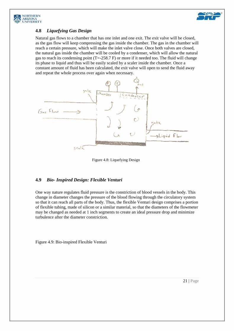
4.8 Liquefying Gas Design
Natural gas flows to a chamber that has one inlet and one exit. The exit valve will be closed,
as the gas flow will keep compressing the gas inside the chamber. The gas in the chamber will
reach a certain pressure, which will make the inlet valve close. Once both valves are closed,
the natural gas inside the chamber will be cooled by a condenser, which will allow the natural
gas to reach its condensing point (T=-258.7 F) or more if it needed too. The fluid will change
its phase to liquid and thus will be easily scaled by a scaler inside the chamber. Once a
constant amount of fluid has been calculated, the exit valve will open to send the fluid away
and repeat the whole process over again when necessary.
Figure 4.8: Liquefying Design
4.9 Bio- Inspired Design: Flexible Venturi
One way nature regulates fluid pressure is the constriction of blood vessels in the body. This
change in diameter changes the pressure of the blood flowing through the circulatory system
so that it can reach all parts of the body. Thus, the flexible Venturi design comprises a portion
of flexible tubing, made of silicon or a similar material, so that the diameters of the flowmeter
may be changed as needed at 1 inch segments to create an ideal pressure drop and minimize
turbulence after the diameter constriction.
Figure 4.9: Bio-inspired Flexible Venturi
22 | Page
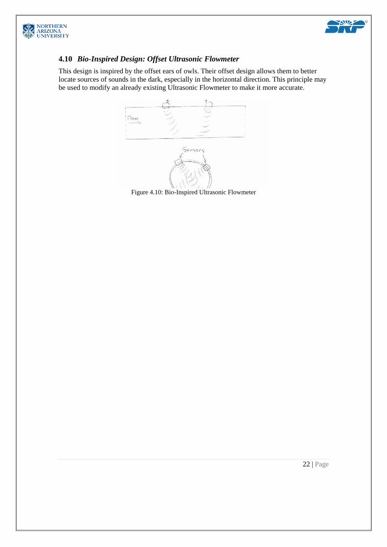
4.10 Bio-Inspired Design: Offset Ultrasonic Flowmeter
This design is inspired by the offset ears of owls. Their offset design allows them to better
locate sources of sounds in the dark, especially in the horizontal direction. This principle may
be used to modify an already existing Ultrasonic Flowmeter to make it more accurate.
Figure 4.10: Bio-Inspired Ultrasonic Flowmeter
23 | Page
5 Designs Selected
In the following section the design(s) that the team has decided to pursue will be discussed.
This section will also discuss the rationale for why the selected design(s) were chosen over
the other design options. There were three designs selected for presentation to the client.
Three designs were selected instead of choosing one in order to leave our options open based
on the feedback we receive from the client. The three designs selected were: improvement of
original system (new FloBoss/ changing diameter of orifice plate), Coriolis meter, and sonic
flowmeter.
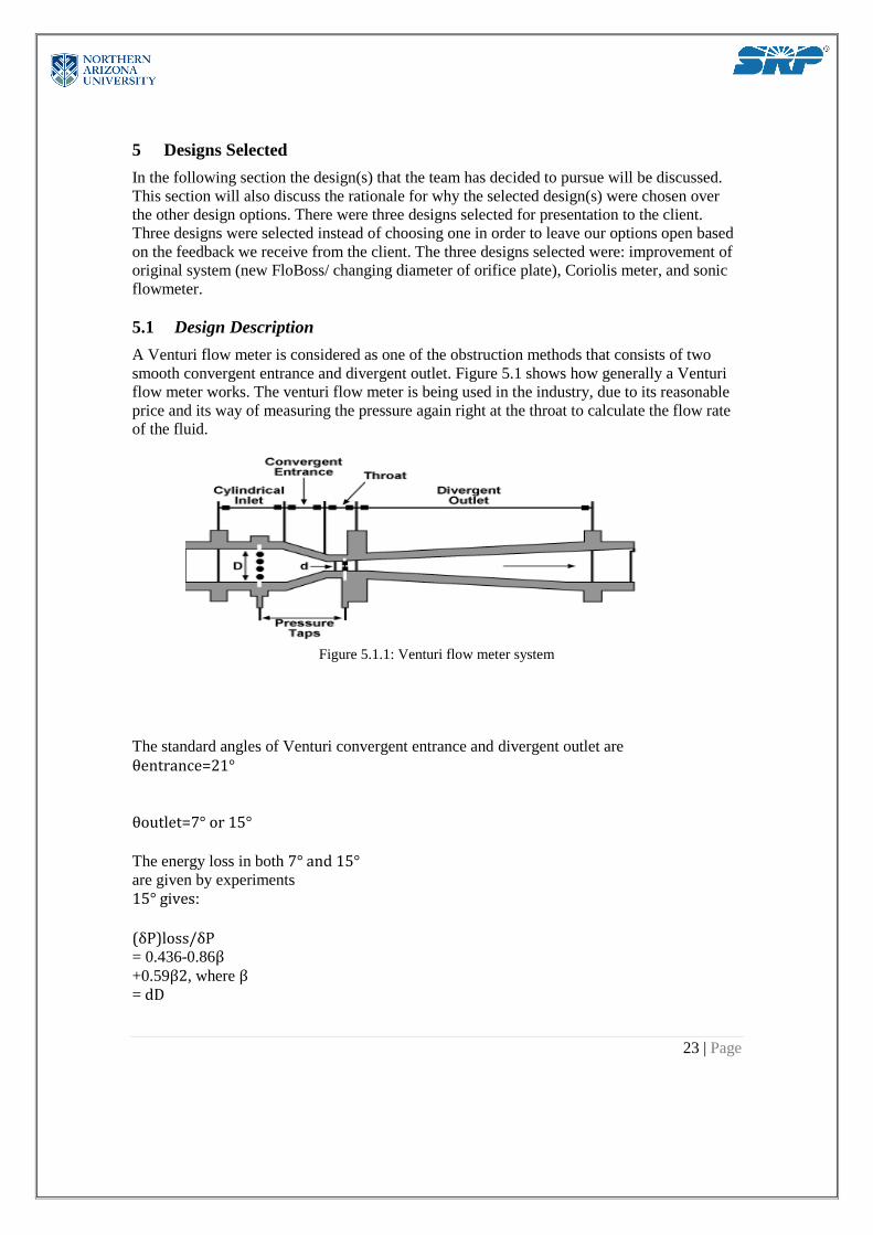
5.1 Design Description
A Venturi flow meter is considered as one of the obstruction methods that consists of two
smooth convergent entrance and divergent outlet. Figure 5.1 shows how generally a Venturi
flow meter works. The venturi flow meter is being used in the industry, due to its reasonable
price and its way of measuring the pressure again right at the throat to calculate the flow rate
of the fluid.
Figure 5.1.1: Venturi flow meter system
The standard angles of Venturi convergent entrance and divergent outlet are θentrance=21°
θoutlet=7° or 15° The energy loss in both 7° and 15° are given by experiments 15° gives:
(δP)loss/δP = 0.436-0.86β +0.59β2, where β = dD
24 | Page
7° gives: (δP)loss/δP = 0.218-0.42β +0.38β2 where β= dD These two equation can be applied on a wide range of Reynold’s numbers, but it can get too
accurate with high Reynold’s numbers that ranges between 2*10^5 < Re < 2*10^6 and 0.4 < B < 0.75, because experimentally, those values will make the Venturi flow meter able to
almost neglect the discharge coefficient “C”. Also the energy loss with this range of reynold’s
numbers will give exactly 10% energy loss with the same range of B. The main equation used
to calculate the flow rate of a compressible flow is
Q=(K*A2*Y/ρ)/(2*g*ρ*∆P)0.5
The assumption made for the design selected has the exact same dimensions for the orifice
plates except that except that the expansion factor Y will be different in a Venturi than an
orifice plate, the calculation made in the appendix is based on many assumptions that can be
accomplished when designing the flow meter. The calculation might be close between the
Venturi and orifice, because it is also assumed that the pressure reading of the venturi is the
same as the orifice, however, in testing the procedure the Venturi should have better readings
than the orifice plate based on the research comparison made between them.
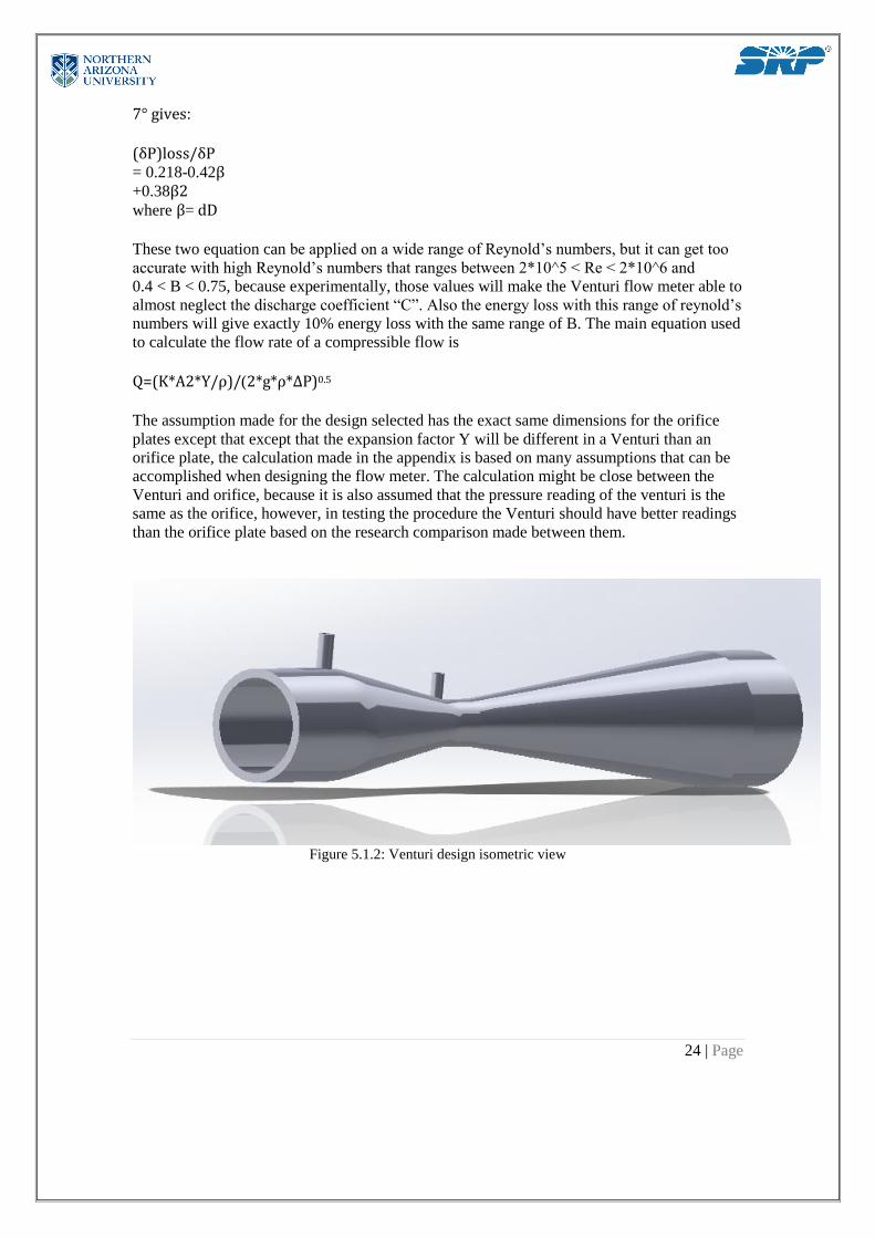
Figure 5.1.2: Venturi design isometric view
25 | Page
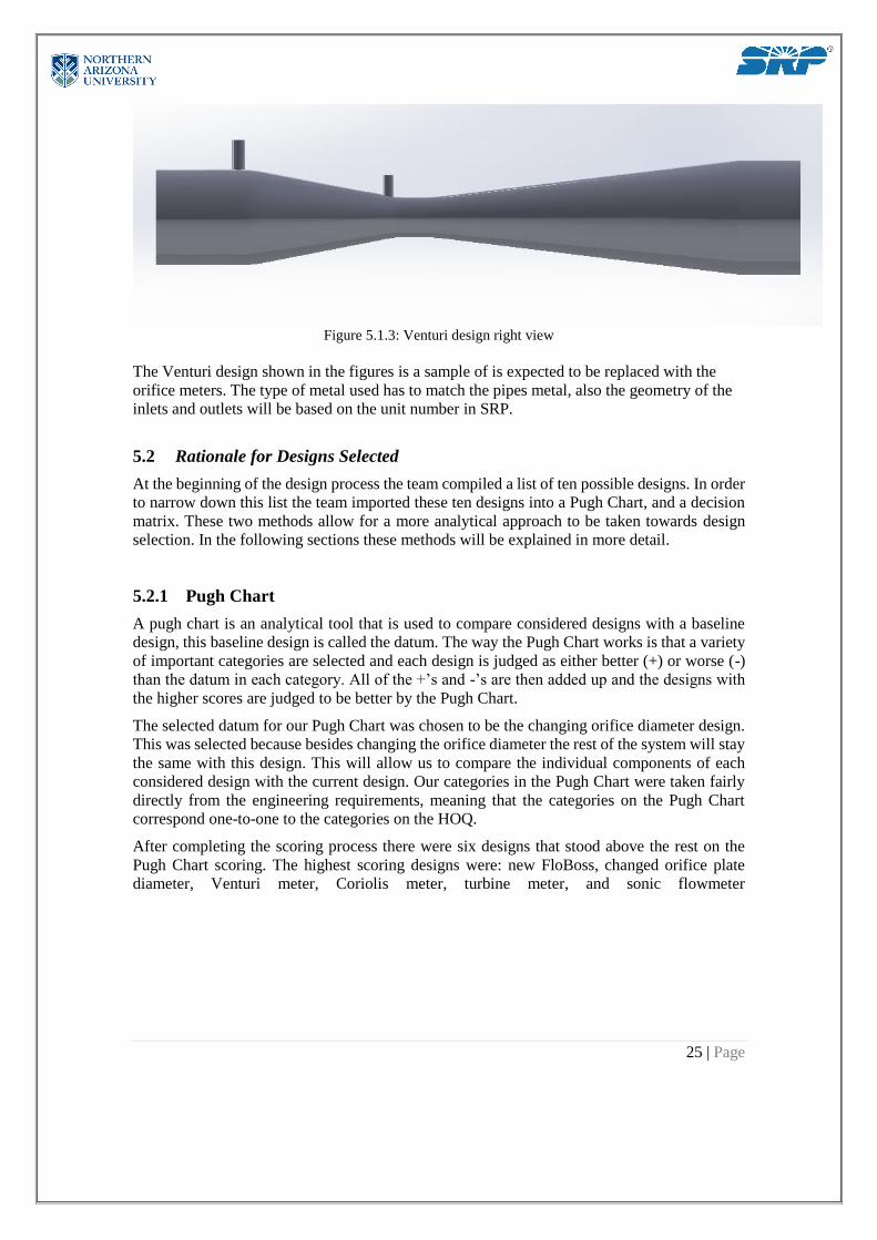
Figure 5.1.3: Venturi design right view
The Venturi design shown in the figures is a sample of is expected to be replaced with the
orifice meters. The type of metal used has to match the pipes metal, also the geometry of the
inlets and outlets will be based on the unit number in SRP.
5.2 Rationale for Designs Selected
At the beginning of the design process the team compiled a list of ten possible designs. In order
to narrow down this list the team imported these ten designs into a Pugh Chart, and a decision
matrix. These two methods allow for a more analytical approach to be taken towards design
selection. In the following sections these methods will be explained in more detail.
5.2.1 Pugh Chart
A pugh chart is an analytical tool that is used to compare considered designs with a baseline
design, this baseline design is called the datum. The way the Pugh Chart works is that a variety
of important categories are selected and each design is judged as either better (+) or worse (-)
than the datum in each category. All of the +’s and -’s are then added up and the designs with
the higher scores are judged to be better by the Pugh Chart.
The selected datum for our Pugh Chart was chosen to be the changing orifice diameter design.
This was selected because besides changing the orifice diameter the rest of the system will stay
the same with this design. This will allow us to compare the individual components of each
considered design with the current design. Our categories in the Pugh Chart were taken fairly
directly from the engineering requirements, meaning that the categories on the Pugh Chart
correspond one-to-one to the categories on the HOQ.
After completing the scoring process there were six designs that stood above the rest on the
Pugh Chart scoring. The highest scoring designs were: new FloBoss, changed orifice plate
diameter, Venturi meter, Coriolis meter, turbine meter, and sonic flowmeter

26 | Page
Figure 5.2.1: Pugh Chart

27 | Page
5.2.2 Decision Matrix
After completing the Pugh Chart there were six designs that scored significantly higher than
the rest, these six designs were then put into a decision matrix. The decision matrix has the
same categories as the Pugh Chart, but in the decision matrix these categories were each
given a weight based on their importance to the success of the design.
The category that was given the highest weight was the ability of the design to decrease the
error in the measurement system. This was given the highest weight because it is imperative
that the design decreases the system error as this is the main project goal. Another important
category was having a low pressure drop across the measurement apparatus. Having a large
pressure drop leads to a larger amount of turbulence which can lead to more error in the
system, in addition a large pressure drop causes greater energy loss, which is an outcome that
should be mitigated as best as possible. Compatibility with the existing system and meeting
EPA/SRP regulations were also major design considerations.

28 | Page
Figure 5.2.2: Decision Matrix
6 Proposed Design
The implementation of our design will be fairly simple. We simply need to purchase 3 units
of our selected flowmeter and then install these three units in the existing fuel measurement
areas in the SRP power plants. So, the only two major costs in the implementation process
will be the cost of purchasing and the cost of installing the system. Pricing for the units was
found using the prices given by AFT instrument for their LGW classic venturi tube. This
listing was found on Alibaba.com [13], a link to the specific listing can be found in the
references section. Cost of installation were assumed using information found online. The
total pricing for the installation is listed in the table below. The total budget for our team was
listed as $3000 so the installation cost will fall within our budget with a margin for error to
account for any unforeseen costs.

29 | Page
Table 6: Installation Costs
Purchasing cost Installation cost Total cost
Per unit $500 $300 $800
Total (3 units) $1500 $900 $2400

30 | Page
7 Implementation
This section will include a brief description of the manufacturing process, as well as the bill
of materials. The bill of materials will describe each item that will be used in the experiment,
along with the items price and manufacturer.
7.1 Manufacturing
For the design of our experiment there was little manufacturing that needed to be done in
terms of machining parts. Instead, all of our individual components were purchased premade
from retailers and the experiment will be assembled by hand by the group members using
basic tools such as hack saws and adhesive tape. A detailed list of all components for our
experiment is listed below in the bill of materials.
7.1.1 Bill of Materials
Table 7.1.1: Bill of Materials
Material Source Cost
Venturi Tube with pressure tap Pasco $150.00
Pasco Airlink Pasco $59.00
6 pressure taps Pasco $100.00
3-D printed nozzle NAU cline library $30.00
Adhesive Tape Home Depot $8.00
20 feet of ¾ in PVC piping Home Depot $7.00
3 straight ¾ in PVC couplers Home Depot $2.50
3 90 degree bend PVC couplers Home Depot $2.50
Washers of various diameter Home Depot $4.50
Total $363.50
As shown in the above table there were two main retailers that the components for the
experiment were purchased from. These retailers were Pasco and Home Depot. Pasco is a
company that mainly specializes in technology used by high school and college educators to
run science experiments. So, they had a plethora of flow sensors and equipment used for flow
measurement at very reasonable prices. For these reasons they were a very good choice to

31 | Page
purchase our electronic flow measurement equipment from. The other major retailer we used
was Home Depot. The equipment we purchased from them was the basic components we are
going to use to construct our piping system. tHe reason they were chosen to purchase our
equipment from is that there is a Home Depot store in close proximity to campus, and the
equipment there is priced extremely inexpensive.
As listed above after all purchasing was completed the total cost come out to $363.50. The
budget for this project given to us by Northern Arizona University is $3,000. The group does
not foresee any more major expenses, so we anticipate that by the end of the project we will
be well within our budget range.
7.2 Design of Experiment
For the final deliverable the team is constructing a lab experiment that simulates SRP’s fuel
measurement system. The lab will be conducted in the thermal fluids lab at Northern Arizona
University (NAU).
7.2.1 Experimental Overview
This lab will test the team’s theory that a Venturi is more accurate than a orifice. This lab will
consist of building an experimental apparatus that fully represents the pipe structure of SRP.
For the piping the team will use various lengths of PVC to test different entry lengths to the
flow meter. The flow meters that will be used in the lab consist of a Venturi tube and a few
different size orifices that all will be tested to see the most accurate flowmeter. For this
experiment the team will be using air from the blower in the thermal fluids lab. To find out
the speed needed to simulate SRP’s fuel system the Reynolds number was scaled from natural
gas to air. This includes changing the viscosity, density, and the diameter, then using the
Reynolds number for SRP’s flow a velocity for air can be calculated. The velocity was found
to be about 23 m/s which is definitely possible to do with the blower. The team is also setting
up a DATUM, an ultrasonic flowmeter to compare with the orifice and Venturi data. The
team will be using a 3D printed nozzle to converge the 4 inch blower to ¾ inch that is needed
for this experiment.
7.2.2 Variables
There are a few variables that are being tested in the lab. One being different orifice diameters
to calculate the more accurate sized orifice. Also being tested are the different bends and
entry lengths leading up to the flow meter to find the more accurate piping geometry. The
Reynolds number is a variable that is being used in the lab experiment. The scaling of the
Reynolds number is important because the team wants to simulate SRP’s fuel system. To do
this the team has calculated the Reynolds number for SRP’s system and compared it to air to
solve for the velocity needed from the blower. Another variable is the pressure drop across
the flow meters, this drop will help the team calculate the accuracy of the flowmeters. The
team will be using the pressure taps and pressure sensor to get values for the pressure drop.
7.2.3 DATUM
The team will use an ultrasonic flowmeter (Uniform 1010P universal portable flowmeter) as
the DATUM for the whole experiment measurements. The team will refer to the Ultrasonic
flowmeter measurements and will compare them to the measurements obtained from the
Venturi flowmeter and the orifice plate flowmeter. The ultrasonic flowmeter will be fixed in

32 | Page
position throughout the multiple trials that the team will perform during the experiment, it
will be positioned just before the bend. This is to guarantee a fully developed flow when
measuring the flow. Based on the results that will be obtained from the ultrasonic flowmeter
the team will perform a statistical and an analytical analysis that will determine the accuracy
of both flowmeters that are being investigated, the orifice plate flowmeter and the Venturi
flowmeter.

33 | Page
7.2.4 Impact of Flow Straightener
Flow straighteners have a strong impact on straightening up undeveloped flows that can
happen after bends or change in the cross-sectional area of pipes. It can provide a fully
developed flow after any bend angle that occurs during piping systems. This method can be
done by placing small circular or quintuple paths inside the required pipe to make the flow
forced to be uniform. The impact that this method can do is significant, especially for pipe
systems that include many bends and cross-sectional area changes. The major benefit out of
flow straighteners is saving space in systems, and making the ability of installing flow meter
at any spot wanted. The reason beyond that is to have flow measurements with a uniform
velocity profile, which will make meters calculate flows easier.
Figure 7.2.4a: Honeycomb flow straighteners
Figure 7.2.4: Honeycomb flow straightener. CAD design.

34 | Page

35 | Page
In the experiment, team 33 will install a flow straightener right after a bend to see how much
it will affect the flow meter readings. The measuring process will be applied twice; the first
one will be without the flow straighteners and the second one will be with them. The readings
should differ, as it will be discussed in the expectations of the experiment, but the main idea
here is to see where is the best length to put the flow meter after installing the flow
straightener inside the pipe. The team will be using the honeycomb flow straighteners as the
method of making flow as developed as possible.
7.2.5 Accuracy of orifice vs. Venturi
This section will include a thorough comparison between the orifice plate meter and the
Venturi. The comparison will be based on the accuracy of both meters, with and without the
flow straightener.
Orifice meter
The orifice meter is a sensitive meter that needs in most cases a long distance before
installation. Due to impact of the diameter ratio on the reading measurement, a big
consideration needed in the length of the straight pipe before the installation of the orifice
meter as shown in the figure (7.2.5a). The length of the straight pipe can be estimated in some
cases, but the main thing is considering the length of that straight pipe and knowing that it
will affect the accuracy of the orifice readings.
Figure 7.2.5a: Orifice meter Diameter ratio.
36 | Page
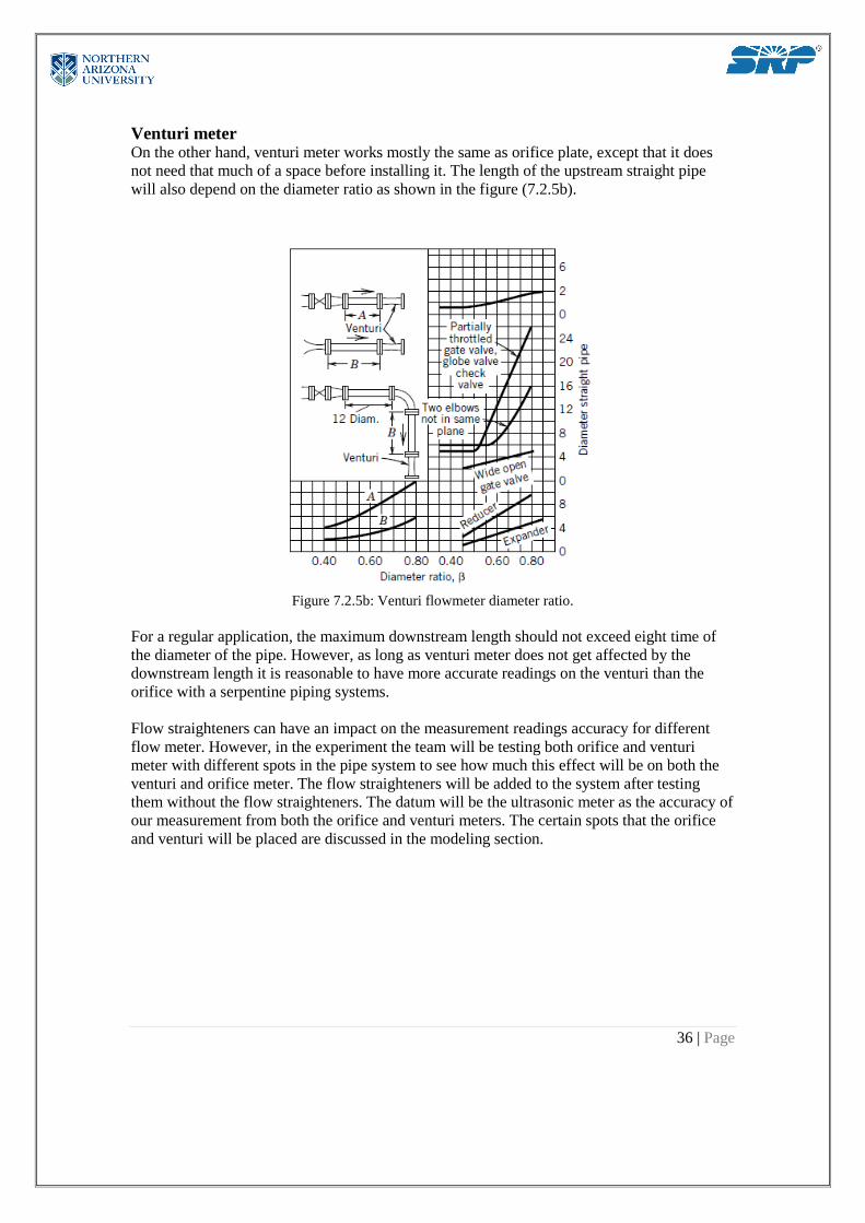
Venturi meter
On the other hand, venturi meter works mostly the same as orifice plate, except that it does
not need that much of a space before installing it. The length of the upstream straight pipe
will also depend on the diameter ratio as shown in the figure (7.2.5b).
Figure 7.2.5b: Venturi flowmeter diameter ratio.
For a regular application, the maximum downstream length should not exceed eight time of
the diameter of the pipe. However, as long as venturi meter does not get affected by the
downstream length it is reasonable to have more accurate readings on the venturi than the
orifice with a serpentine piping systems.
Flow straighteners can have an impact on the measurement readings accuracy for different
flow meter. However, in the experiment the team will be testing both orifice and venturi
meter with different spots in the pipe system to see how much this effect will be on both the
venturi and orifice meter. The flow straighteners will be added to the system after testing
them without the flow straighteners. The datum will be the ultrasonic meter as the accuracy of
our measurement from both the orifice and venturi meters. The certain spots that the orifice
and venturi will be placed are discussed in the modeling section.
37 | Page
7.2.6 Impact of orifice diameter
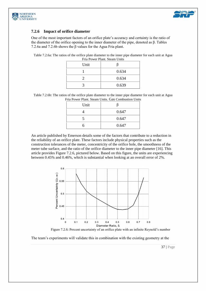
One of the most important factors of an orifice plate’s accuracy and certainty is the ratio of
the diameter of the orifice opening to the inner diameter of the pipe, denoted as β. Tables
7.2.6a and 7.2.6b shows the β values for the Agua Fria plant.
Table 7.2.6a: The ratios of the orifice plate diameter to the inner pipe diameter for each unit at Agua
Fria Power Plant. Steam Units
Unit β
1 0.634
2 0.634
3 0.639
Table 7.2.6b: The ratios of the orifice plate diameter to the inner pipe diameter for each unit at Agua
Fria Power Plant. Steam Units. Gas Combustion Units
Unit β
4 0.647
5 0.647
6 0.647
An article published by Emerson details some of the factors that contribute to a reduction in
the reliability of an orifice plate. These factors include physical properties such as the
construction tolerances of the meter, concentricity of the orifice hole, the smoothness of the
meter tube surface, and the ratio of the orifice diameter to the inner pipe diameter [16]. This
article provides Figure 7.2.6, pictured below. Based on this figure, the units are experiencing
between 0.45% and 0.46%, which is substantial when looking at an overall error of 2%.
Figure 7.2.6: Percent uncertainty of an orifice plate with an infinite Reynold’s number
The team’s experiments will validate this in combination with the existing geometry at the

38 | Page
plant by testing orifice plates with different sized bore holes.
39 | Page
7.2.7 Impact of pipe geometry
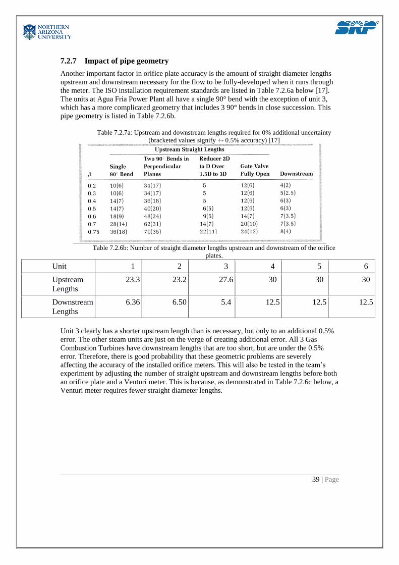
Another important factor in orifice plate accuracy is the amount of straight diameter lengths
upstream and downstream necessary for the flow to be fully-developed when it runs through
the meter. The ISO installation requirement standards are listed in Table 7.2.6a below [17].
The units at Agua Fria Power Plant all have a single 90° bend with the exception of unit 3,
which has a more complicated geometry that includes 3 90° bends in close succession. This
pipe geometry is listed in Table 7.2.6b.
Table 7.2.7a: Upstream and downstream lengths required for 0% additional uncertainty
(bracketed values signify +- 0.5% accuracy) [17]
Table 7.2.6b: Number of straight diameter lengths upstream and downstream of the orifice
plates.
Unit 1 2 3 4 5 6
Upstream
Lengths
23.3 23.2 27.6 30 30 30
Downstream
Lengths
6.36 6.50 5.4 12.5 12.5 12.5
Unit 3 clearly has a shorter upstream length than is necessary, but only to an additional 0.5%
error. The other steam units are just on the verge of creating additional error. All 3 Gas
Combustion Turbines have downstream lengths that are too short, but are under the 0.5%
error. Therefore, there is good probability that these geometric problems are severely
affecting the accuracy of the installed orifice meters. This will also be tested in the team’s
experiment by adjusting the number of straight upstream and downstream lengths before both
an orifice plate and a Venturi meter. This is because, as demonstrated in Table 7.2.6c below, a
Venturi meter requires fewer straight diameter lengths.
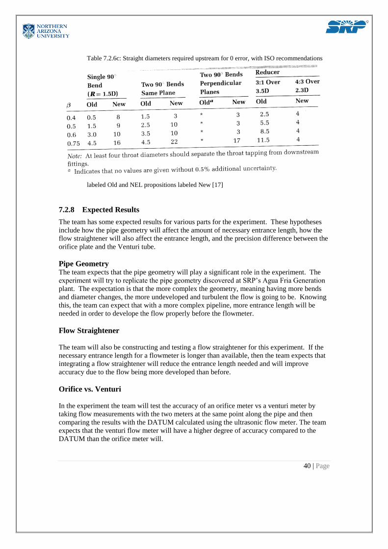
40 | Page
Table 7.2.6c: Straight diameters required upstream for 0 error, with ISO recommendations
labeled Old and NEL propositions labeled New [17]
7.2.8 Expected Results
The team has some expected results for various parts for the experiment. These hypotheses
include how the pipe geometry will affect the amount of necessary entrance length, how the
flow straightener will also affect the entrance length, and the precision difference between the
orifice plate and the Venturi tube.
Pipe Geometry
The team expects that the pipe geometry will play a significant role in the experiment. The
experiment will try to replicate the pipe geometry discovered at SRP’s Agua Fria Generation
plant. The expectation is that the more complex the geometry, meaning having more bends
and diameter changes, the more undeveloped and turbulent the flow is going to be. Knowing
this, the team can expect that with a more complex pipeline, more entrance length will be
needed in order to develope the flow properly before the flowmeter.
Flow Straightener
The team will also be constructing and testing a flow straightener for this experiment. If the
necessary entrance length for a flowmeter is longer than available, then the team expects that
integrating a flow straightener will reduce the entrance length needed and will improve
accuracy due to the flow being more developed than before.
Orifice vs. Venturi
In the experiment the team will test the accuracy of an orifice meter vs a venturi meter by
taking flow measurements with the two meters at the same point along the pipe and then
comparing the results with the DATUM calculated using the ultrasonic flow meter. The team
expects that the venturi flow meter will have a higher degree of accuracy compared to the
DATUM than the orifice meter will.

41 | Page
8 Testing
9 Conclusion
The mission for this project encompassed improving the fuel measurement accuracy of the
flow meter system of the Aqua Fria SRP power plant. This was done by researching various
types of flow meters and common sources of error to recommend options to our client. An
experiment was conducted testing these parameters by simulating the SRP plant’s fuel
measurement system. Which consisted of testing the effect of different size orifice diameters,
a flow straightener, upstream pipe length, and a Venturi tube vs. orifice plate. The team ran a
precision analysis on the data taken to concur our hypothesis of these common errors. The
team proposed to the client all the options that would reduce the error along with which
option would be more cost efficient and decrease error. SRP liked the options that were
presented and decided to look more into the Venturi tube option with the backup choice being
installing a flow straightener.
The main ground rules were that our team would be professional and organized. The project
success was due to the professional and adequate work put in by the whole team. All
members were willing to put their best effort into the researching, designing, manufacturing
and testing that went into the outcome of this project. All team members completed their
work according to the deadlines that were set for each assignment. To stay organized
everything was copied to google docs so all members could review all documents that have
been completed throughout the two semesters. Since the ground rules were followed the
outcome of the project was a success ending up with SRP liking the options proposed. The
coping strategies involved solutions to conflicts that would arise throughout the project. There
were no huge issues that arisen that needed coping, the team worked extremely well together
which is portrayed by the outcome of the project.
[Question 3] The project had many positives to its completion when talking about the
performance of the project itself. Communication between the team members was a crucial
aspect to keep ahead of deadlines and the team did a great job of accomplishing a high level
of communication. This allowed each team member to understand exactly where the other
team members where they were within their parts of the project tasks and allowed questions
and concerns to be answered quickly and accurately. Time management was another well
done aspect from each of the team members as the team decided, most of the time, to make
deadlines earlier than the university’s deadlines. This allowed the team some recovery time in
order to fix any issues with any deliverables as well as having some time to correctly format
and proofread the deliverables as well. As for the experiment itself a major positive was that
the expected results were the results that the team came up with at the end of the experiment.
This was reassuring as the team did not run into any unexpected results and thus did not have
to backtrack and reassess the experiment. As the team decided to scale down the experiment
using PVC pipe the manufacturing costs of the project was very low as most of the material as
most of the material was able to be purchased at local hardware stores. This low cost allowed
the team to be able to purchase higher end sensors in order to get more precise readings which
allowed for a more detailed precision analysis. The project did not go perfectly smooth as
there was some issues that arose during the project’s length.
42 | Page
[Question 4] Some negative aspects to the project arose during this year-long project. The
first of these was the distance between the university and the power plant that was the team’s
project location. This lead to only a few visits where the team needed to be efficient with
their visits in order to get all the information to move forward. This also lead to not as much
communication between the team and power plant and its representatives as the team would
of liked and some confusion because of this. In the beginning of the project the lack of
communication to the client representative lead to some confusion about what exactly the
goal and the overall issue was with the power plant at first. Additionally with a project of this
size is done the lack of an actual physical product can throw the team off, especially when
other teams have a actual product and can see progress. This was, at first, a concern for the
team as the team did not know where they stood on the progression of the project. Once the
team came to terms that the deliverable was not an actual product but results of an experiment
instead the team was able to shift their focus onto designing an experiment, performing an
experiment, and finally analyzing the results in order to determine trends and relationships
between various variables within the experiment. Many tools and methods allowed the team
to accomplish the various tasks that the university and the clients gave the team.
[Question 6]The team has encountered many problems throughout the whole project. The
first problems that the team faced were finding the reason behind the accuracy error, but this
problem was solved by performing some intensive research on flow meters and power plants
in general. The team has found many factors that can affect the measurement of the flow
meter. Another problem the team faced was to replicate the piping system in Agua Fria power
plant. With this being said, the team had to perform a non-dimensionlisation analysis to the
parameters and factors that were collected during the experiment.
One problem that the team could not find a solution for was having a datum to compare the
accuracy between the orifice plate and the venturi flow meters. The datum had to be either a
very accurate meter (less than accuracy) or an ultrasonic meter. The ultrasonic was the meter
used by the supplier. Having an accurate flow meter would make it easier to compare the
measurement of both the flow meters. Unfortunately, the ultrasonic flow meter was expensive
and exceeded our allocated budget. The team had to change the analysis from an accuracy
analysis to a precision analysis, that can be related straight forward to the accuracy analysis.
The team also encountered a problem in terms of having sufficient data to analyze form the
company itself.
[Question 7] The team did a very good job of utilizing Google Drive services to keep all of
our different documents separate and organized. Using this as an organizational tool helped to
allow teammates to contribute to the completion of documents remotely when they were not
able to be present at group meetings. Something that would have helped the group in terms of
organization would have been to have some sort of schedule available online that detailed
when the group was planning on meeting for the next few weeks. We used group text
messages as well as word of mouth to determine when meetings would take place which
sometimes led to group members being mistaken or unaware of meeting times.
[Question 8] Finally, the team learned how to effectively formulate an engineering problem
and explore solutions from an engineering perspective. This awareness, both theoretically and
practically, is crucial in the engineering profession because it defines what engineers are
trained to do, which is solving problems using simple yet effective approaches. Currently, the
team can identify an existing engineering concern and then compose equations and
hypotheses that could solve the problem. With this being said, the team explored various flow
meters and investigated the operating principles behind each flow meter. In addition, the team
explored the operational system that controls power plants, and also how power plants
actually operate. The technical communication skills that were developed as a result of
communicating with professional engineers was very beneficial in terms of getting the team
43 | Page
ready for their professional careers.
References
[1] M. Duzen, "Turnkey natural gas measurement," in flowcontrolnetwork.com, Flow Control
Network, 2014. [Online]. Available: http://www.flowcontrolnetwork.com/turnkey-natural-
gas-measurement/. Accessed: Sep. 20, 2016.
[2] "How gas turbine power plants work,". [Online]. Available: http://energy.gov/fe/how-gas-
turbine-power-plants-work. Accessed: Sep. 25, 2016.
[3] G. Electric, "Combined-cycle power plant – how it works | GE power generation," in
Power Generation, 2016. [Online]. Available:
https://powergen.gepower.com/resources/knowledge-base/combined-cycle-power-plant-how-
it-works.html. Accessed: Sep. 25, 2016.
[4] J. Mollerup and P. Angelo, "Measurement and correlation of the volumetric properties of
a synthetic natural gas mixture", Fluid Phase Equilibria, vol. 19, no. 3, pp. 259-271, 1985
[5]"» The Transportation of Natural Gas NaturalGas.org", Naturalgas.org, 2016. [Online].
Available: http://naturalgas.org/naturalgas/transport/. [Accessed: 28- Sep- 2016].
[6]"Combustion Engine for Power Generation- Introduction", Wartsila.com, 2016. [Online].
Available: http://www.wartsila.com/energy/learning-center/technical-
comparisons/combustion-engine-for-power-generation-introduction. [Accessed: 30- Sep-
2016].
[7]"EIA - Natural Gas Pipeline Network - Transportation Process & Flow", Eia.gov, 2016.
[Online]. Available:
https://www.eia.gov/pub/oil_gas/natural_gas/analysis_publications/ngpipeline/process.html.
[Accessed: 30- Sep- 2016].
[8] "Coriolis mass flow measuring principle Archives - Instrumentation
Tools", Instrumentation Tools, 2016. [Online]. Available:
http://instrumentationtools.com/tag/coriolis-mass-flow-measuring-principle/. [Accessed: 27-
Oct- 2016].
[9] "Types of Fluid Flow Meters", Engineeringtoolbox.com, 2016. [Online]. Available:
http://www.engineeringtoolbox.com/flow-meters-d_493.html. [Accessed: 27-Oct- 2016].
[10] “Webtec – Hydraulics,” Webtec.com, 2016. [Online]. Available:
http://www.webtec.com/en/tech/reports/turbine. [Accessed: 29- Oct- 2016].
[11] Emerson, “FloBoss 107E Flow Manager” [Online} Available:
http://www2.emersonprocess.com/en-
US/brands/FloBoss/gasflowcomputers/107E/Pages/107E.aspx. [Accessed 25-Oct-2016]

44 | Page
[12]"Gas turbine engines -", Petrowiki.org, 2016. [Online]. Available:
http://petrowiki.org/Gas_turbine_engines. [Accessed: 29- Sep- 2016].
[13]"Venturi tube Flowmeter to measure gas," www.alibaba.com, 1999. [Online]. Available:
https://www.alibaba.com/product-detail/venturi-tube-flowmeter-to-measure-
gas_1233261483.html. Accessed: Nov. 22, 2016.

45 | Page
[14] R. S. Figliola and D. E. Beasley, Theory and design for mechanical measurements, 3rd
ed. New York, NY: John Wiley and Sons (WIE), 2000.
[15] T. G. Beckwith, Roy D., and John H., Mechanical Measurements, fifth edition ed. United
States: Addison Wesley, 1995
[16] J. P. Holman, Holman, and Search our Used & Out of... Holman, Solutions manual to
accompany experimental methods for engineers, sixth edition, 6th ed. New York: McGraw Hill Higher Education, 1993
[17] Emerson (2010). Theoretical Uncertainty of Orifice Flow Measurement [Online].
ETA Process Instrumentation.
[18] R. C. Baker, “Orifice Plate Meters” & “Venturi Meter and Standard Nozzles,” in Flow
Measurement Handbook: Industrial Designs, Operating Principles, Performance, and
Applications, Cambridge, UK: Cambridge, 2000, ch. 5 & 6, pp. 95-139.

46 | Page
Appendix A
Matlab codes for flow rate calculations in orifice plate and Venturi.
clc clear
%These equations can be applied on obsturction meters (orifice &
venturi)%
%fluid's composition% Nitrogen=[0.31 0.31 0.31 0.32 0.32 0.31 0.31 0.31 0.31 0.31] %changes
at unit#4&5% CO2=[1.28 1.28 1.28 1.28 1.28 1.28 1.28 1.28 1.28 1.28] %constant% Methane=[97.23 97.23 97.23 97.22 97.22 97.23 97.23 97.23 97.23 97.23]
%changes at unit#4&5% Ethane=[0.93 0.93 0.93 0.93 0.93 0.93 0.93 0.93 0.93 0.93] %constant% Propane=[0.19 0.19 0.19 0.19 0.19 0.19 0.19 0.19 0.19 0.19]
%constant% nButane=[0.02 0.02 0.02 0.02 0.02 0.02 0.02 0.02 0.02 0.02]
%constant% iButane=[0.03 0.03 0.03 0.03 0.03 0.03 0.03 0.03 0.03 0.03]
%constant% nPentane=[0 0 0 0 0 0 0 0 0 0] %constant% iPentane=[0 0 0 0 0 0 0 0 0 0] %conastant% Hexane=[0.01 0.01 0.01 0.01 0.01 0.01 0.01 0.01 0.01 0.01] %constant% Heptane=[0 0 0 0 0 0 0 0 0 0] %constant% Octane=[0 0 0 0 0 0 0 0 0 0] %constant% Nonane=[0 0 0 0 0 0 0 0 0 0] %constant% Decane=[0 0 0 0 0 0 0 0 0 0] %constant% H2S=[0 0 0 0 0 0 0 0 0 0] %constant% Water=[0 0 0 0 0 0 0 0 0 0] %constant% Helium=[0 0 0 0 0 0 0 0 0 0] %constant% Oxygen=[0 0 0 0 0 0 0 0 0 0] %constant% CO=[0 0 0 0 0 0 0 0 0 0] %constant% Hydrogen=[0 0 0 0 0 0 0 0 0 0] %constant%
%meters setup%
n=[1 2 3 4 5 6 7 8 9 10] %unit#1-#10% density_air=1.23 %density of air at T=15 celsius in kg/m^3% patm=14.12841 %atmospheric pressure in psi% g=32.11277 %gravitational accelaration ft/s^2% Mu=0.6 %viscosity in cp% density=[1.588 2.083 0.001 11.895 11.906 11.935 5.734 5.753 5.757
5.778] %denstiy at each orifice plate in kg/m^3%
%http://unitrove.com/engineering/tools/gas/natural-gas-density%
%changing the givens to SI units%

47 | Page
SG=0.5758 %specific gravity for all units% k=1.3 %specific heat ratio for all units% Patm=97411.957886 %atmospheric pressure in pa for all units% G=9.787972296 %gravitational accelaration in m/s^2 for all the units% MU=0.0006 %viscosity in N.s/m^2% Density=SG*density_air %density of natural gas from specific of
gravity in kg/m^3% R=0.287058 %gas constant of natural gas in KJ/Kg*k%
d0=[8.8712 8.8759 10.2199 3.883 3.883 3.883 2.3748 4.9988 6.0003
7.0009] %orifice diameter in inches for all units (flow meters)% d1=[14 14 16 6 6 6 4.023 11.937 11.941 11.937] %pipe diameter in
inches for all units (flow meters)%
D0=d0.*0.0254 %diameter in m% D1=d1.*0.0254 %diameter in m%
B=D0./D1 %diameters coefficient%
A0=(pi./4).*D0.^2 %orifice plate cross-section area in m^2 for all
units (flow meters)% A1=(pi./4).*D1.^2 %pipe cross-section area in m^2 for all units (flow
meters)%
E=1./sqrt(1-B.^4) %coefficient%
Delta_p=[0.0671479 -0.0842513 0.0420168 0.0167982 -0.0336361 -
0.0757066 0.0587801 0.0503626 -0.0168554 -0.0084084] %change in
pressure in inH2O for all units (flow meters)% p1=[32.89332 43.31176 0.0269687 246.2265 246.1623 246.1391 125.3776
125.5657 125.6203 125.6866] %static pressure in psi for all units
(flow meters)%
Delta_P=Delta_p.*249.088875 %change in pressure in pa% P1=p1.*6894.75729 %static pressure in pa% P2=P1-abs(Delta_P) %pressure after orifice plate in pa%
Tf=[58.48682 60.05267 65.5163 71.51623 70.9614 69.74372 91.4132
90.4752 90.43119 88.81457] %flow tempreture in Fehrenheit for all
units (flow meters)% Tc=(Tf-32)*(5/9) %flow tempreture in celsius for all units (flow
meters)% Tk=Tc+273.15 %flow tempreture in kelvin for all units (flow meters)%
%flow rate for incompressible flow% C=0.965 %discharge coefficient% %0.95<C<0.98 for venturi%
%C=Q_actual/Q_ideal% K=C*E %coefficient%

48 | Page
Q_ideal=(A0./sqrt((1-
(A0./A1).^2))).*sqrt((2.*G.*abs(Delta_P))./Density) %Ideal flow rate
at each orifice plate in m^3/s 'incompressible flow assumption'% Q_actual=(K.*A0).*sqrt(2.*G./Density).*sqrt(abs(Delta_P)) %actual
flow rate at each orifice plate in m^3/s 'incompressible flow
assumption'% M=Q_actual.*Density %mass flow rate in kg/s% v1=Q_actual./A1 %velocity of natural gas before entering the orifice
plate in m/s% v2=Q_actual./A0 %velocity of natural gas after entering the orifice
plate in m/s%
Q_ft=Q_actual.*35.3146667 %flow rate in each orifice plate in ft^3/s% Q1_ft=Q_ideal.*35.3146667
TD=max(Q_actual)./min(Q_actual) %the turndown of orifice plate%
c=sqrt(k.*R.*Tk) %speed of sound in m/s at each unit% Ma=v1./c %Mach number for all units (flow meters)% Re_d1=(Density.*v1.*D1)./MU %Reynold's number of pipes for all units
(flow meters)% hL=(abs(Delta_P)./Density) %head losses of orifice plate in KJ/KG for
all units (flow meters)%
%flow rate for compressible flow in orifice plate% Y=1-(0.41+0.35.*B.^4).*(abs(Delta_P)./(k.*P1)) %Expansion factor for
orifice plates% Q_c_actual=((Y.*K.*A0)./Density).*sqrt(2.*G.*Density.*abs(Delta_P))
%Actual flow rate for the compressible flow in m^3/s%
Q_c_ft=Q_c_actual.*35.3146667 %flow rate in each orifice plate in
ft^3/s%
%flow rate for compressible flow in venturi% Y1=((P2./P1).^(2./k).*(k./(k-1)).*((1-(P2./P1).^((k-1)./k))./(1-
(P2./P1))).*((1-B.^4)./(1-B.^4.*(P2./P1).^(2./k)))).^0.5 %Expansion
factor for venturi% Q_c1_actual=((Y1.*K.*A0)./Density).*sqrt(2.*G.*Density.*abs(Delta_P))
%Actual flow rate for the compressible flow in m^3/s%
Q_c1_ft=Q_c1_actual.*35.3146667 %flow rate in each orifice plate in
ft^3/s%
diffrence_between_orifice_and_venturi_pecentage=((Q_c_ft-
Q_c1_ft)./Q_c_ft).*100

49 | Page
%Assumptions made%
%B for venturi is the same as Orifice plate% %Density of natural gas% %Gas constant of natural gas 'R'% %dischage coefficient 'C'% %venturi pressure readings are the same as orifice pressure readings%


