
Adaptive Trajectory Control for
Autonomous Helicopters
Eric N. Johnson∗ and Suresh K. Kannan†
School of Aerospace Engineering, 270 Ferst Drive,
Georgia Institute of Technology, Atlanta, GA 30332-0150
For autonomous helicopter flight, it is common to separate the flight
control problem into an inner loop that controls attitude and an outer loop
that controls the translational trajectory of the helicopter. In previous
work, dynamic inversion and neural-network-based adaptation was used
to increase performance of the attitude control system and the method
of pseudocontrol hedging (PCH) was used to protect the adaptation pro-
cess from actuator limits and dynamics. Adaptation to uncertainty in the
attitude, as well as the translational dynamics, is introduced, thus minimiz-
ing the effects of model error in all six degrees of freedom and leading to
more accurate position tracking. The PCH method is used in a novel way
that enables adaptation to occur in the outer loop without interacting with
the attitude dynamics. A pole-placement approach is used that alleviates
timescale separation requirements, allowing the outer loop bandwidth to
be closer to that of the inner loop, thus, increasing position tracking per-
formance. A poor model of the attitude dynamics and a basic kinematics
model is shown to be sufficient for accurate position tracking. The theory
and implementation of such an approach, with a summary of flight test
results, are described.
∗Lockheed Martin Assistant Professor of Avionics Integration, AIAA Member,[email protected]
†Research Assistant. AIAA Student Member, suresh [email protected]
1 of 49
Adaptive Trajectory Control for Autonomous Helicopters, JOHNSON and KANNAN
I. Nomenclature
A,B error dynamics system matrices
A1, A2, B estimate of vehicle dynamics as a linear system
a, a acceleration, activation potential
a(·), a(·) translational dynamics and its estimate
bv, bw neural network (NN) biases
e reference model tracking error
g(·), g(·) actuator dynamics and its estimate
K, R inner loop, outer loop gain matrices
n1, n2, n3 number of NN inputs, hidden neurons, outputs
P,Q Lyapunov equation matrices
p, p position, roll rate
q, q attitude quaternion, pitch rate
r, r filtered tracking error, yaw rate
V, W,Z NN input, output, both weights
v velocity
x state vector
xin, x NN input
zj input to jth hidden neuron
α angular acceleration
α(·), α(·) attitude dynamics and its estimate
∆(·) error the NN can approximate
∆(·) total function approximation error
δ, δ actuator deflections and its estimate
εg(·), εg error NN cannot approximate and its bound
ζ error dynamics damping
θv,θw NN input-layer, output-layer thresholds
νad adaptive signal
νr robustifying term
ω, ω angular velocity, error dynamics bandwidth
A. Subscripts
ad adaptive
c commanded
coll, ped collective, pedal
2 of 49
Adaptive Trajectory Control for Autonomous Helicopters, JOHNSON and KANNAN
cr reference model dynamics
d derivative
des desired
f force
h hedge
i, o inner loop, outer loop
lat, lon lateral, longitudinal
m moment
p proportional
r robustifying term, reference model
II. Introduction
Unmanned helicopters are versatile machines that can perform aggressive maneuvers.
This is evident from the wide range of acrobatic maneuvers executed by expert pilots. He-
licopters have a distinct advantage over fixed-wing aircraft especially in an urban environ-
ment, where hover capability is helpful. There is increased interest in the deployment of
autonomous helicopters for military applications, especially in urban environments. These
applications include reconnaissance, tracking of individuals or other objects of interest in a
city, and search and rescue missions in urban areas. Autonomous helicopters must have the
capability of planning routes and executing them. To be truly useful, these routes would in-
clude high-speed dashes, tight turns around buildings, avoiding dynamic obstacles and other
required aggressive maneuvers. In planning1 these routes, however, the tracking capability
of the flight control system is a limiting factor because most current control systems still do
not leverage the full flight envelope of small helicopters, at least, unless significant system
identification and validation has been conducted.
Although stabilization and autonomous flight2 has been achieved, the performance has
generally been modest compared to a human pilot. This may be attributed to many fac-
tors, such as parametric uncertainty (changing mass, and aerodynamic characteristics), un-
modeled dynamics, actuator magnitude and rate saturation and assumptions made during
control design itself. Parametric uncertainty limits the operational envelope of the vehicle to
where control designs are valid, whereas unmodeled dynamics and saturation can severely
limit the achievable bandwidth of the system. The effect of uncertainty and un-modeled
dynamics have been successfully handled using a combination of system identification3–5
and robust control techniques.6 Excellent flight and simulation results have been reported
including acrobatic maneuvers7 and modestly aggressive maneuvers.6,8
3 of 49
Adaptive Trajectory Control for Autonomous Helicopters, JOHNSON and KANNAN
A key aspect in the effective use of unmanned aerial vehicles(UAVs) for military and civil
applications is their ability to accommodate changing dynamics and payload configurations
automatically without having to rely on substantial system identification efforts. Neural-
Network (NN) based direct adaptive control has recently emerged as an enabling technology
for practical flight control systems that allow online adaptation to uncertainty. This tech-
nology has been successfully applied to the recent U.S. Air Force Reconfigurable Control for
Tailless Fighter Aircraft (RESTORE) culminating in a successful flight demonstration9,10 of
the adaptive controller on the X-36. A combined inner-outer loop architecture was also ap-
plied for guidance and control of the X-33 (Ref. 11) and evaluated successfully in simulation
for various failure cases.
This paper is concerned with the development of an adaptive controller for an autonomous
helicopter using a neural network as the adaptive element. For autonomous helicopters, a
primary objective is the accurate tracking of position commands. Much adaptive control
work on helicopters has concentrated on improving the tracking performance of attitude
commands.12–14 Usually a simple outer loop employing basic relationships between attitude
and linear acceleration is then used to control the translational dynamics. For many appli-
cations this may be sufficient. However, when operating in an urban environment or flying
in formation with other UAVs, the position tracking ability of the controller dictates the
minimum proximity between the UAV and objects in its environment. In contrast to previ-
ous attitude control-only work, we introduce a coupled inner-outer loop adaptive design that
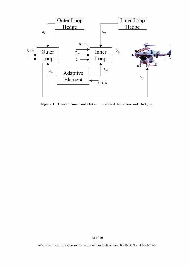
can handle uncertainty in all six degrees of freedom. In synthesizing a controller (Fig. 1),
the conventional conceptual separation between the inner loop and outer loop is made. The
inner loop controls the moments acting on the aircraft by changing the lateral stick, δlat,
longitudinal stick, δlon and pedal, δped, inputs. The outer loop controls the forces acting on
the aircraft by varying the magnitude of the rotor thrust using the collective δcoll input. The
thrust vector is effectively oriented in the desired direction by commanding changes to the
attitude of the helicopter using the inner loop.
The attitude and translational dynamics are input-state feedback linearized separately
using dynamic inversion and linear controllers designed for the linearized dynamics. The
effect of nonlinear parametric uncertainty arising due to approximate inversion is minimized
using an adaptive element. A nonlinearly parameterized NN will be used to provide on-line
adaptation. The design is such that actuator saturation limits are not avoided or prevented.
When an adaptive element is introduced, a new problem arises by way of unwanted adapta-
tion to plant input characteristics such as actuator saturation and dynamics. For example,
the inner-loop attitude control sees actuator limits, rate saturation and associated dynamics.
To alleviate this problem, pseudocontrol hedging11,15 (PCH), is used to modify the inner-
loop reference model dynamics in a way that allows continued adaptation in the presence of
4 of 49
Adaptive Trajectory Control for Autonomous Helicopters, JOHNSON and KANNAN
these system characteristics. This same technique, PCH, is used to prevent adaptation to
inner-loop dynamics and interaction between the inner and outer loops. Without hedging of
the outer loop, adaptation to uncertainty in the translational dynamics would not be possi-
ble. A common assumption when designing control systems for air vehicles is the timescale
separation16 between the inner-loop attitude control and outer-loop trajectory control sys-
tems. The assumption allows the inner loop and outer loop to be designed separately but
requires the outer-loop bandwidth to be much lower than that of the inner loop. This prob-
lem is alleviated by using a combination of PCH and gain selection by a combined analysis
of the two loops. This allows the outer-loop bandwidth to be closer to that of the inner loop,
thus increasing position tracking performance. Additionally, to the authors knowledge, the
flight results presented in this paper are the first where adaptation is used to compensate
for modeling errors in all six degrees of freedom.
We first develop the adaptive controller architecture for a generic six-degree-of-freedom
air vehicle, followed by a description of the NN and selection of linear compensator gains. The
controller is then applied to the trajectory and attitude control of an unmanned helicopter.
Practical discussions on the choice of parameters and reference model dynamics are provided.
Finally, flight test results are presented.
III. Controller Development
Consider an air vehicle modeled as a nonlinear system of the form
p = v (1)
v = a(p, v, q,ω, δf , δm) (2)
q = q(q,ω) (3)
ω = α(p,v, q, ω, δf , δm) (4)
where, p ∈ R3 is the position vector, v ∈ R3 is the velocity of the vehicle, q ∈ R4 is the
attitude quaternion and ω ∈ R3 is the angular velocity. Eq. (2) represents translational
dynamics and Eq. (4) represents the attitude dynamics. Eq. (3) represents the quaternion
propagation equations.17 The use of quaternions, though not a minimal representation of
attitude, avoids numerical and singularity problems that Euler angles based representations
have. This enables the control system to be all attitude capable as required for aggressive
maneuvering. The state vector x may now be defined as
x ,[pT vT qT ωT
]T
(5)
5 of 49
Adaptive Trajectory Control for Autonomous Helicopters, JOHNSON and KANNAN
The control vectors are denoted by δf and δm and represent actual physical actua-
tors on the aircraft, where δf denotes the primary force generating actuators and δm de-
notes the primary moment generating actuators. For a helicopter, the main force effec-
tor is the rotor thrust which is controlled by changing main rotor collective δcoll. Hence
δf ∈ R1 = δcoll. There are three primary moment control surfaces, the lateral cyclic
δlat, longitudinal cyclic δlon, and tail rotor pitch, also called the pedal input δped. Hence,
δm ∈ R3 =[δlat δlon δped
]T
. This classification of the controls as moment and force gen-
erating, is an artefact of the inner-loop–outer-loop control design strategy. In general, both
control inputs, δf and δm, may each produce forces and moments. The helicopter is an
under-actuated system, and hence, the aircraft’s attitude, q, is treated like a virtual actua-
tor used to tilt the main rotor thrust in order to produce desired accelerations. Defining the
consolidated control vector δ as
δ ,[δT
f δTm
]T
(6)
the actuators themselves may have dynamics represented by
δ =
δm
δf
=
gm(x, δm, δmdes
)
gf (x, δf , δfdes)
= g(x, δ, δdes) (7)
where g(·) is assumed to be asymptotically stable but perhaps unknown.
When any actuator dynamics and nonlinearities are ignored, approximate feedback lin-
earization of the system represented by (1,2,3,4) is achieved by introducing the following
transformation: ades
αdes
=
a(p, v, q,ω, qdes, δfdes
, δm)
α(p,v, q,ω, δf , δmdes)
(8)
where, ades,αdes are commonly referred to as the pseudocontrol and represent desired ac-
celerations. Here, a, α represent an available approximation of a(·) and α(·). Additionally,
δfdes, δmdes
, qdes are the control inputs and attitude that are predicted to achieve the desired
pseudo-control. This form assumes that translational dynamics are coupled strongly with
attitude dynamics, as is the case for a helicopter. From the outer-loop’s point of view, q (at-
titude), is like an actuator that generates translational accelerations and qdes is the desired
attitude that the outer-loop inversion expects will contribute towards achieving the desired
translational acceleration, ades. The dynamics of q appears like actuator dynamics to the
outer loop. The attitude quaternion qdes will be used to augment the externally commanded
attitude qc to achieve the desired translational accelerations. Because actuator positions
are often not measured on small helicopters, estimates of the actuator positions δm, δf are
used. For cases where the actuator positions are directly measured, they may be regarded
6 of 49
Adaptive Trajectory Control for Autonomous Helicopters, JOHNSON and KANNAN
as known δm = δm and δf = δf . In fact, in the outer loop’s case, the attitude q is measured
using inertial sensors. When a and α are chosen such that they are invertible, the desired
control and attitude may be written as
δfdes
qdes
= a−1(p,v, q,ω, ades, δm)
δmdes= α−1(p, v, q,ω, δf ,αdes) (9)
where actuator estimates are given by actuator models
˙δ =
˙δf
˙δm
=
gf (x, δf , δfdes
)
gm(x, δm, δmdes)
= g(x, δ, δdes) (10)
In later sections, it will be shown that α, can just be an approximate linear model of vehicle
attitude dynamics and a a set of simple equations relating translational accelerations to the
attitude of the vehicle. Introducing the inverse control law Eq. (9) into Eq. (2) and Eq. (4)
results in the following closed-loop translational and attitude dynamics
v = ades + ∆a(x, δ, δ)− ah
ω = αdes + ∆α(x, δ, δ)−αh (11)
where
∆(x, δ, δ) =
∆a(x, δ, δ)
∆α(x, δ, δ)
=
a(x, δ)− a(x, δ)
α(x, δ)− α(x, δ)
(12)
are static nonlinear functions (model error) that arise due to imperfect model inversion and
errors in the actuator model g. The signals, ah and αh, represent the pseudocontrol that
cannot be achieved due to actuator input characteristics such as saturation. If the model
inversion were perfect and no saturation were to occur, ∆, ah and αh would vanish leaving
only the pseudocontrols ades and αdes. One may address model error and stabilize the
linearized system by designing the pseudocontrols as
ades = acr + apd − aad
αdes = αcr + αpd − αad (13)
where acr and αcr are outputs of reference models for the translational and attitude dynamics
respectively. apd and αpd are outputs of proportional-derivative (PD) compensators; and
finally, aad and αad are the outputs of an adaptive element (an NN) designed to cancel
7 of 49
Adaptive Trajectory Control for Autonomous Helicopters, JOHNSON and KANNAN
model error ∆. The effects of input dynamics, represented by ah, αh will first be addressed
in the following section by designing the reference model dynamics such that they do not
appear in the tracking error dynamics. The reference model, tracking error dynamics and
adaptive element are discussed in the following sections.
A. Reference Model and PCH
Normally, the reference model dynamics are of the form
pr = vr
vr = acr(pr, vr, pc, vc)
qr = q(qr,ωr)
ωr = αcr(qr,ωr, qc ⊕ qdes, ωc) (14)
where pr and vr are the outer-loop reference model states whereas qr, ωr, are the inner-loop
reference model states. The external command signal is xc =[pT
c vTc qT
c ωTc
]T
. Note
that the attitude desired by the outer loop is now added to the commands for the inner loop
controller. Here, qc ⊕ qdes denotes quaternion addition.17
Any dynamics and nonlinearities associated with the actuators δm, δf have not yet been
considered in the design. If they become saturated (position or rate), the reference models
will continue to demand tracking as though full authority were still available. Furthermore,
the inner loop appears like an actuator with dynamics to the outer loop. Practical operational
limits on the maximum attitude of the aircraft may have also been imposed in the inner-
loop reference model. This implies that the outer-loop desired attitude augmentation qdes
may not actually be achievable, or at the very least is subject to the inner-loop dynamics.
When an adaptive element such as a neural network is introduced, these input dynamics and
nonlinearities will appear in the tracking error dynamics resulting in the adaptive element
attempting to correct for them and is undesirable.
Pseudocontrol hedging may be used to prevent the adaptive element from attempting
to adapt to selected system input characteristics. One way to describe the PCH method is
as follows: Move the reference models in the opposite direction (hedge) by an estimate of
the amount the plant did not move due to system characteristics the control designer does
not want the adaptive element to see.15 This will prevent the characteristic from appearing
in the model tracking error dynamics to be developed in the sequel. The reference model
8 of 49
Adaptive Trajectory Control for Autonomous Helicopters, JOHNSON and KANNAN
dynamics may be redesigned to include hedging as follows
vr = acr − ah
ωr = αcr −αh (15)
acr = acr(pr, vr,pc,vc)
αcr = αcr(qr,ωr, qc ⊕ qdes, ωc) (16)
where ah and αh are the difference between commanded pseudocontrol and achieved pseu-
docontrol.
ah = a(x, qdes, δfdes, δm)− a(x, δf , δm)
= ades − a(x, δf , δm) (17)
αh = α(x, δf , δmdes)− α(x, δf , δm)
= αdes − α(x, δf , δm) (18)
Note that the hedge signals ah, αh, do not directly affect the reference model output acr,
αcr, but do so only through subsequent changes in the reference model states.
Remark 1. Choosing the reference model dynamics acr and αcr is important in determining
the effect of actuator saturation on the system dynamics.18,19
B. Tracking error dynamics
One may define the tracking error vector, e, as
e ,
pr − p
vr − v
Q(qr, q)
ωr − ω
(19)
where, Q : R4 × R4 7→ R3, is a function15 that, given two quaternions results in an error
angle vector with three components. An expression for Q is given by
Q(p, q) = 2sgn(q1p1 + q2p2 + q3p3 + q4p4)×−q1p2 + q2p1 + q3p4 − q4p3
−q1p3 − q2p4 + q3p1 + q4p2
−q1p4 + q2p3 − q3p2 + q4p1
(20)
9 of 49
Adaptive Trajectory Control for Autonomous Helicopters, JOHNSON and KANNAN
The output of the PD compensators may be written as
apd
αpd
=
Rp Rd 0 0
0 0 Kp Kd
e (21)
where, Rp, Rd ∈ R3×3, Kp, Kd ∈ R3×3 are linear gain positive definite matrices whose choice
is discussed below. The tracking error dynamics may be found by directly differentiating
Eq. (19).
e =
vr − v
vr − v
ωr − ω
ωr − ω
(22)
Considering e2,
e2 = vr − v
= acr − ah − a(x, δ)
= acr − ades + a(x, δ)− a(x, δ)
= acr − apd − acr + aad + a(x, δ)− a(x, δ)
= −apd − (a(x, δ)− a(x, δ)− aad)
= −apd − (∆a(x, δ, δ)− aad)
(23)
e4 may be found similarly. Then, the overall tracking error dynamics may now be expressed
as
e = Ae + B[νad − ∆(x, δ, δ)
](24)
where, ∆ is given by Eq. (12),
νad =
aad
αad
(25)
A =
0 I 0 0
−Rp −Rd 0 0
0 0 0 I
0 0 −Kp −Kd
, B =
0 0
I 0
0 0
0 I
(26)
and so the linear gain matrices must be chosen such that A is Hurwitz. Now, νad remains
to be designed in order to cancel the effect of ∆.
Remark 2. (a) Note that commands, δmdes, δfdes
, qdes, do not appear in the tracking error
10 of 49
Adaptive Trajectory Control for Autonomous Helicopters, JOHNSON and KANNAN
dynamics. PCH allows adaptation to continue when the actual control signal has been re-
placed by any arbitrary signal. (b) If the actuator is considered ideal and the actual position
and the commanded position are equal, addition of the PCH signal ah, αh has no effect on
any system signal.
C. Effect of Actuator Model on Error Dynamics
An important aspect of the PCH signal calculation given by Eq. (17) and Eq. (18) is esti-
mation of the actual actuator position at the current instant. The assumptions and model
used to estimate the actuator positions in calculating the hedging signals play a role in what
appears in the tracking error dynamics.
1. Actuator Positions are Measured
The simplest case arises when δ is measured and available for feedback. In this case, mod-
els for the actuators are not needed. In fact, when all actuator signals are known then
∆(x, δ, δ) = ∆(x, δ) = ∆(x, δ) and the tracking error dynamics of Eq. (24) is given by
e = Ae + B [νad(x, δ)−∆(x, δ)] (27)
Note that with regard to the outer loop, the inner loop acts like an actuator with dynamics,
at least with respect to achieving the desired attitude qdes. The actual attitude quaternion,
q, is available and appears as a part of the state measurement. Hence, it is always available
as an input to the adaptive element as well as in the calculation of the hedge signal.
2. Actuator Position is a Static Function of the Model and Plant States
If it can be assumed that actuator deflections have the form δ = δ(x, δ), for example,
saturation occurs earlier than in the model of the actuator, the discrepancy appears as
model error which the NN can correct for. Thus, ∆(x, δ(x, δ), δ) = ∆(x, δ) and the error
dynamics take the form
e = Ae + B[νad(x, δ)−∆(x, δ)
](28)
3. Actuator model has error the NN cannot compensate
If actuator positions are not measured and an assumption such as δ = δ(x, δ) cannot be
made, the uncertainty ∆ may be expressed as
∆(x, δ, δ) = ∆(x, δ) + εg(x, δ, δ) (29)
11 of 49
Adaptive Trajectory Control for Autonomous Helicopters, JOHNSON and KANNAN
where, ∆(x, δ) is model error the NN can approximate and εg is the model error the NN
cannot cancel when δ is not available as an input to the network and has components
independent of x and δ. Errors in the actuator model that the NN can cancel include bias
error in the actuator position estimate and erroneous values for when magnitude saturation
occurs. Model errors that appear in εg which the neural network cannot cancel include
parameters that affect the dynamics of the actuator such as actuator time constants and
rate limits. The tracking error dynamics may now be expressed as
e = Ae + B[νad(x, δ)−∆(x, δ)− εg(x, δ, δ)
](30)
where, νad(x, δ) is designed to cancel ∆(x, δ) and εg appears as unmodeled input dynamics
to the control system.
4. Actuator model is conservative
One way to predict actuator position accurately is to impose conservative artificial limits on
the desired actuator deflections, perhaps in software and make the assumption that the real
actuator tracks the conservative commands accurately. This amounts to always knowing δ,
and the error dynamics take the form given by Eq. (27).
Thus far, the various components of Eq. (13) have been designed and PCH has been
used to prevent any input dynamics from appearing in the error dynamics of Eq. (24). The
only component yet to be designed is the adaptive element νad(.) to approximate ∆(.) and
minimize the forcing term on the right hand side of the error dynamics equations. In this
paper, a single hidden layer NN is used, its structure and approximation capabilities are
discussed in the following section.
D. Adaptive Element
Single hidden layer (SHL) perceptron NNs are universal approximators.20–22 Hence, given a
sufficient number of hidden layer neurons and appropriate inputs, it is possible to train the
network online to cancel model error. Fig. 2 shows the structure of a generic single hidden
layer network whose input-output map may be expressed as
νadk= bwθwk
+
n2∑j=1
wjkσj(zj) (31)
12 of 49
Adaptive Trajectory Control for Autonomous Helicopters, JOHNSON and KANNAN
where, k = 1, ..., n3, bw is the outer layer bias, θwkis the kth threshold. wjk represents the
outer layer weights and the scalar σj is a sigmoidal activation function
σj(zj) =1
1 + e−azj(32)
where, a is the so called activation potential and may have a distinct value for each neuron.
zj is the input to the jth hidden layer neuron, and is given by
zj = bvθvj+
n1∑i=1
vijxini(33)
where, bv is the inner layer bias and θvjis the jth threshold. Here, n1, n2 and n3 are the
number of inputs, hidden layer neurons and outputs respectively. xini, i = 1, ..., n1, denotes
the inputs to the NN. For convenience, define the following weight matrices:
V ,
θv,1 · · · θv,n2
v1,1 · · · v1,n2
.... . .
...
vn1,1 · · · vn1,n2
(34)
W ,
θw,1 · · · θw,n3
w1,1 · · · w1,n3
.... . .
...
wn2,1 · · · wn2,n3
(35)
Z ,
V 0
0 W
(36)
Additionally, define the σ(z) vector as
σT (z) ,[bw σ(z1) · · · σ(zn2)
](37)
where bw > 0 allows for the thresholds, θw, to be included in the weight matrix W . Also,
z = V T x, where,
xT =[bv xT
in
](38)
where, bv > 0, is an input bias that allows for thresholds θv to be included in the weight
matrix V . The input-output map of the SHL network may now be written in concise form
13 of 49
Adaptive Trajectory Control for Autonomous Helicopters, JOHNSON and KANNAN
as
νad = W T σ(V T x) (39)
The NN may be used to approximate a nonlinear function, such as ∆(.). The universal
approximation property20 of NN’s ensures that given an ε > 0, then ∀ x ∈ D, where D is
a compact set, ∃ an n2 and an ideal set of weights (V ∗,W ∗), that brings the output of the
NN to within an ε-neighborhood of the function approximation error. This ε is bounded by
ε which is defined by
ε = supx∈D
∥∥W T σ(V T x)−∆(x)∥∥ (40)
The weights, (V ∗,W ∗) may be viewed as optimal values of (V, W ) in the sense that they
minimize ε on D. These values are not necessarily unique. The universal approximation
property thus implies that if the NN inputs xin are chosen to reflect the functional depen-
dency of ∆(·), then ε may be made arbitrarily small given a sufficient number of hidden
layer neurons, n2.
The adaptive signal νad actually contains two terms
νad = νad + νr =
aad + ar
αad + αr
(41)
where νad is the output of the SHL NN described earlier. For an air vehicle with adaptation
in all degrees of freedom, νad ∈ R6, where the first three outputs, aad, approximates ∆a
and the last three outputs, αad, approximate ∆α and is consistent with the definition of the
error in Eq. (19). νr = [aTr , αT
r ]T ∈ R6 is a robustifying signal that arises in the proof of
boundedness.
IV. Boundedness
Associated with the tracking error dynamics given in Eq. (24), is the Lyapunov function.
AT P + PA + Q = 0 (42)
Choosing positive definite15
Q =
Q1 0
0 Q2
1
14n2 + b2
w
(43)
14 of 49
Adaptive Trajectory Control for Autonomous Helicopters, JOHNSON and KANNAN
where,
Q1 =
RdR
2p 0
0 RdRp
> 0 (44)
Q2 =
KdK
2p 0
0 KdKp
> 0 (45)
Making use of the property that Rp, Rd, Kp, Kd > 0 and diagonal, results in a positive definite
solution for P . Hence,
P =
P1 0
0 P2
1
14n2 + b2
w
(46)
where,
P1 =
R2
p + 12RpR
2d
12RpRd
12RpRd Rp
> 0 (47)
P2 =
K2
p + 12KpK
2d
12KpKd
12KpKd Kp
> 0 (48)
The inputs to the NN have to be chosen to satisfy the functional dependence of ∆(x, δ) and
may be specified as
xT =[bv xT
in
]
xTin =
[xT
c eTr eT νT
ad ‖Z‖F
] (49)
Assumption 1. The norm of the ideal weights (V ∗,W ∗) is bounded by a known positive
value,
0 < ‖Z∗‖F ≤ Z (50)
where, ‖ · ‖F denotes the Frobenius norm.
Assumption 2. The external vehicle state command xc is bounded,
‖xc‖ ≤ xc (51)
Assumption 3. The states of the reference model, remain bounded for permissable plant
15 of 49
Adaptive Trajectory Control for Autonomous Helicopters, JOHNSON and KANNAN
and actuator dynamics. Hence,
‖er‖ ≤ er (52)
Assumption 4. The model error arising from using a dynamic model to estimate actuator
position εg is assumed to be bounded as
‖εg‖ ≤ εg (53)
Assumption 5. Note that, ∆ depends on νad through the pseudo-controls ades,αdes, whereas
νad has to be designed to cancel ∆. Hence the existence and uniqueness of a fixed-point-
solution for νad = ∆(x,νad) is assumed. Sufficient conditions23 for this assumption are also
available.
Theorem 1. Consider the system given by (1,2,3,4) together with the inverse law (9) and
assumptions (1,2,3,4,5), where
r = (eT PB)T (54)
νad = νad + νr (55)
νad = W T σ(V T x) (56)
νr = −Kr(‖Z‖F + Z)‖e‖‖r‖r (57)
with diagonal Kr > 0 ∈ R6×6, and where W,V satisfy the adaptation laws
W = − [(σ − σ′V T x)rT + κ‖e‖W ]
ΓW (58)
V = −ΓV
[x(rT W T σ′) + κ‖e‖V ]
(59)
with ΓW , ΓV > 0 and scalar κ > 0, guarantees that reference model tracking error e and NN
weights (W,V ) are uniformly ultimately bounded.
Proof. See appendix.
Corollary 1. All plant states p,v, q,ω are uniformly ultimately bounded.
Proof. If the ultimate boundedness of e,W, V from Theorem 1 is taken together with As-
sumption 3, the uniform ultimate boundedness of the plant states is immediate following the
definition of the reference model tracking error in Eq. (19).
V. Application to an Autonomous Helicopter
Consider the application of the combined inner-outer-loop adaptive architecture to the
trajectory control of a helicopter. The dynamics3,5, 24 of the helicopter may be modeled in the
16 of 49
Adaptive Trajectory Control for Autonomous Helicopters, JOHNSON and KANNAN
same form as Eqns. (1-4). Most small helicopters include a Bell-Hiller stabilizer bar, which
provides provide lagged rate feedback, and is a source of unmodeled dynamics. The nonlinear
model used for simulation in this work included the stabilizer bar dynamics. Additionally,
blade flapping and other aspects such as gear and engine dynamics were also modeled.
A. Approximate Model
An approximate model for the attitude dynamics of the helicopter was generated by lin-
earizing the nonlinear model around hover and neglecting coupling between the attitude and
translational dynamics as well as the stabilizer bar.
αdes = A1
p
q
r
+ A2
u
v
w
+ B
δlat
δlon
δped
︸ ︷︷ ︸des
−
δlat
δlon
δped
︸ ︷︷ ︸trim
(60)
or,
αdes = A1ωB + A2vB + B(δmdes− δmtrim
) (61)
where, A1 and A2 represent the attitude and translational dynamics respectively, ωB repre-
sents the angular velocity of the body with respect to the earth expressed in the body frame.
vB, is the body velocity vector with respect to the earth expressed in the body frame. δmtrim
is the trim control vector that is consistent with the linear model. Choosing the control
matrix B such that it is invertible, the moment controls may be evaluated as
δmdes= B−1(αdes − A1ωB − A2vB) + δmtrim
(62)
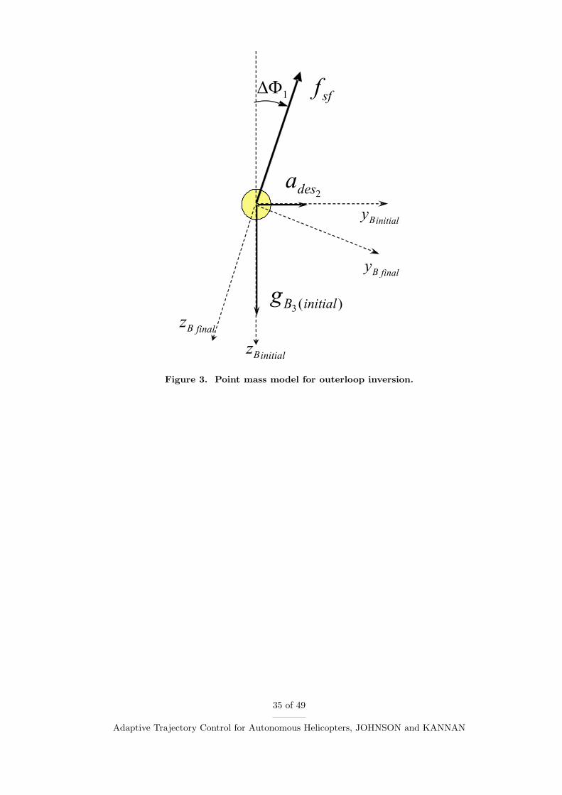
The translational dynamics were modelled as a point mass with a thrust vector that may
be oriented in a given direction as illustrated in Fig. 3. More involved inverses25 may be
used, but the simple relationships between thrust, attitude and accelerations suffice when
used with adaptation.
ades =
0
0
Zδcoll
(δcolldes
− δcolltrim) + Lbvg (63)
where, Zδcollis the control derivative for acceleration in the vertical axis. Lbv is the direction
cosine matrix that transforms a vector from the vehicle (or local) frame to the body frame
17 of 49
Adaptive Trajectory Control for Autonomous Helicopters, JOHNSON and KANNAN
and g is an assumed gravity vector. The desired specific force along the body z axis may be
evaluated as
fsf = (ades − Lbvg)3 (64)
The required collective input may be evaluated as
δcolldes=
fsf
Zδcoll
+ δcolltrim(65)
The attitude augmentation required in order to orient the thrust vector to attain the desired
translational accelerations are given by the following small angle corrections from the current
reference body attitude and attitude command
∆Φ1 =ades2
fsf
, ∆Φ2 = −ades1
fsf
, ∆Φ3 = 0 (66)
For this simplified helicopter model, heading change has no effect on accelerations in the x, y
plane and hence ∆Φ3 = 0. These three correction angles may now be used to generate the
attitude quaternion correction desired by the outer loop. Thus,
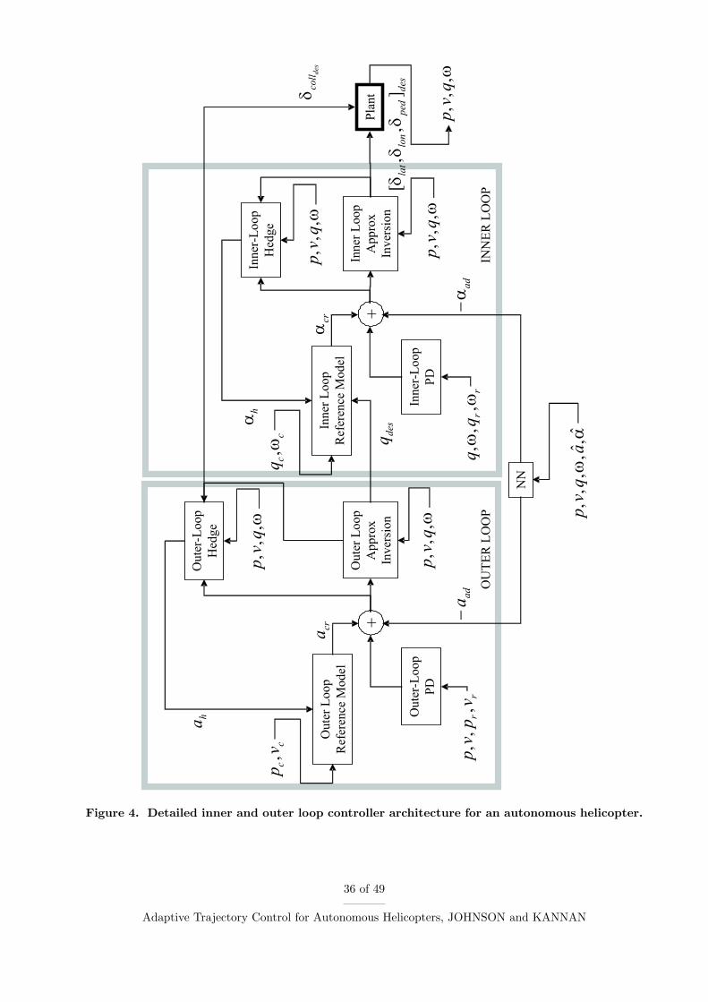
qdes = q(∆Φ1, ∆Φ2, ∆Φ3) (67)
where, q(.) is a function17 that expresses an euler-angles-based rotation as a quaternion. The
overall detailed controller architecture is shown in Fig. 4.
Remark 3. If the desired specific force fsf is close to zero, which occurs when the desired
acceleration in the body z axis is the same as the component of gravity vector along that axis,
then, Equation (66) is undefined. To overcome this problem, one can impose a restriction
where (66) is only computed if |fsf | > fsf , where fsf > 0 and is a lower limit. Essentially it
means, do not bother using attitude unless the desired specific force is greater than fsf .
B. Reference Model
A reasonable choice for the reference model dynamics is given by
acr = Rp(pc − pr) + Rd(vc − vr)
vr = acr − ah (68)
αcr = Kp(Q(qc ⊕ qdes, qr)) + Kd(ωc − ωr)
ωr = αcr −αh (69)
18 of 49
Adaptive Trajectory Control for Autonomous Helicopters, JOHNSON and KANNAN
where, Rp, Rd, Kp, Kd are the same gains used for the PD compensator in Eq. (21). If limits
on the angular rate or translational velocities are to be imposed, then they may be easily
included in the reference model dynamics by modifying acr and αcr to the following form
acr = Rd[vc − vr + sat(R−1d Rp(pc − pr), vlim)]
αcr = Kd[ωc − ωr + sat(K−1d KpQ, ωlim)] (70)
where the functional dependence of Q has been dropped for clarity and is the same as in
Eq. (69). The function sat(·) is the saturation function and vlim, ωlim are the translational
and angular rate limits respectively.
Remark 4. Note that there are no limits placed on the externally commanded position,
velocity, angular rate or attitude. For example, in the translational reference model, if a
large position step is commanded, pc = [1000, 0, 0]T ft and vc = [0, 0, 0]T ft/s, the speed
at which this large step will be achieved is vlim. On the other hand if pc =∫
vcdt and
vc = [60, 0, 0]T ft/s, the speed of the vehicle will be 60ft/s. Similarly, ωlim dictates how fast
large attitude errors will be corrected. Additionally, aggressiveness with which translational
accelerations will be pursued by tilting the body may be governed by limiting the magnitude
of qdes to the scalar limit qlim.
C. Choice of Gains Rp, Rd, Kp, Kd
When the combined adaptive inner-outer-loop controller for position and attitude control
is implemented, the poles for the combined error dynamics must be selected appropriately.
The following analysis applies to the situation where inversion model error is compensated
for accurately by the NN and we assume that the system is exactly feedback linearized. The
inner loop and outer loop each represent a second order system and the resulting position
dynamics p(s)/pc(s) are fourth order in directions perpendicular to the rotor spin axis.
When the closed-loop longitudinal dynamics, near hover, are considered, and with an
acknowledgment of an abuse of notation, it may be written as
x = ades = xc + Rd(xc − x) + Rp(xc − x) (71)
θ = αdes = θg + Kd(θg − θ) + Kp(θg − θ) (72)
where, Rp, Rd, Kp and Kd are the PD compensator gains for the inner loop (pitch angle)
and outer loop (fore-aft position). Now x is now the position, θ the attitude and θg the
attitude command. Normally, θg = θc + θdes where θc is the external command and θdes
the outer-loop-generated attitude command. Here, we assume that the external attitude
command and its derivatives are zero; hence, θg = θdes. In the following development, the
19 of 49
Adaptive Trajectory Control for Autonomous Helicopters, JOHNSON and KANNAN
transfer function x(s)/xc(s) is found and used to place the poles of the combined inner-outer
loop system in terms of the PD compensator gains.
When contributions of θg(s) and θg(s), are ignored, the pitch dynamics Eq. (72) may be
rewritten in the form of a transfer function as
θ(s) =θ(s)
θg(s)θg(s) =
Kp
s2 + Kds + Kp
θg(s) (73)
If the outer-loop linearizing transformation used to arrive at Eq. (71) has the form x = fθ,
where f = −g and g is gravity, it may be written as,
s2x(s) = fθ(s) (74)
The outer-loop attitude command may be generated as
θdes =xdes
f=
ades
f(75)
Note that θg = θdes; if θc = 0,
θg = θdes =1
f[xc + Rd(xc − x) + Rp(xc − x)] (76)
When Eq. (73) and Eq. (76) are used in Eq. (74),
s2x(s) =Kp [s2xc + Rds(xc − x) + Rp(xc − x)]
s2 + Kds + Kp
(77)
Rearranging the above equation results in the following transfer function
x(s)
xc(s)=
Kps2 + KpRds + KpRp
s4 + Kds3 + Kps2 + KpRds + KpRp
(78)
One way to choose the gains is by examining a fourth-order characteristic polynomial
written as the product of two second order systems.
Υ(s) = (s2 + 2ζoωo + ω2o)(s
2 + 2ζiωi + ω2i )
= s4 + (2ζiωi + 2ζoωo)s3
+ (ω2i + 4ζoωoζiωi + ω2
o)s2
+ (2ζoωoω2i + 2ω2
oζiωi)s + ω2oω
2i (79)
where, the subscripts i, o, represent the inner and outerloop values respectively.
Comparing the coefficients of the poles of Eq. (78) and Eq. (79) allows the gains to be
20 of 49
Adaptive Trajectory Control for Autonomous Helicopters, JOHNSON and KANNAN
expressed as a function of the desired pole locations for each axis in turn
Rp =ω2
oω2i
ω2i + 4ζoωoζiωi + ω2
o
Rd = 2ωoωi(ζoωi + ωoζi)
ω2i + 4ζoωoζiωi + ω2
o
Kp = ω2i + 4ζoωoζiωi + ω2
o
Kd = 2ζiωi + 2ζoωo (80)
D. Imposing Response Characteristics
One method6,14 to evaluate the performance of the control system is to use the metrics given
in Aeronautical Design Standard-33 (Ref. 26) handling qualities specifications. When there
is no saturation the hedging signals ah,αh are zero. When it is assumed that the adaptation
has reached its ideal values of (V ∗,W ∗), then
v = acr + apd + εa
ω = αcr + αpd + εα (81)
where εa and εα are bounded by ε. Additionally, the Lyapunov analysis provides guaranteed
model following, which implies apd and αpd are small. Thus, v ≈ acr and ω ≈ αcr. Hence,
as long as the preceding assumptions are valid over the bandwidth of interest, the desired
response characteristics may be encoded into the reference model acr and αcr.
VI. Results
The proposed guidance and control architecture was applied to the Georgia Institute of
Technology Yamaha R-Max helicopter (GTMax) shown in Fig. 5. The basic GTMax he-
licopter weighs about 157lb and has a main rotor radius of 5.05ft. Nominal rotor speed
is 850 revolutions per minute. Its practical payload capability is about 66lbs with a flight
endurance of greater than 60 minutes. It is also equipped with a Bell-Hillier stabilizer bar.
Its avionics package includes a Pentium 266 flight control computer, an inertial measurement
unit (IMU), a global positioning system, a 3-axis magnetometer and a sonar altimeter. The
control laws presented in this paper were first implemented in simulation27 using a nonlinear
helicopter model that included flapping and stabilizer bar dynamics. Wind and gust models
were also included. Additionally, models of sensors with associated noise characteristics were
implemented. Many aspects of hardware such as the output of sensor model data as serial
packets was simulated. This introduced digitization errors as would exist in real-life and also
21 of 49
Adaptive Trajectory Control for Autonomous Helicopters, JOHNSON and KANNAN
allowed testing of many flight specific components such as sensor drivers.28 The navigation
system consists of a 17-state Kalman filter to estimate variables such as attitude, and terrain
altitude. The navigation filter was executed at 100Hz and corresponds to the highest rate
at which the IMU is able to provide data. Controller calculations occurred at 50Hz. The
control laws were first implemented as C-code and tested in simulation. Because almost all
aspects specific to flight-testing were included in the simulation environment, a subset of
the code from the simulation environment was implemented on the main flight computer.
During flight, ethernet and serial based data links provided a link to the ground station
computer that allowed monitoring and uploading of way-points. A simple kinematics-based
trajectory generator (with limits on accelerations) was used to generate smooth consistent
trajectories (pc, vc, qc,ωc) for the controller. Various moderately aggressive maneuvers were
performed during flight to test the performance of the trajectory-tracking controller. Testing
of the controller began with simple hover followed by step responses and way-point naviga-
tion. Following initial flight tests, aggressiveness of the trajectory was increased by relaxing
acceleration limits in the trajectory generator and relaxing ωlim and vlim in the reference
models. Tracking error performance was increased by increasing the desired bandwidth of
the controllers. Selected results from these flight tests are provided in the following sections.
A. Parameter Selections
The controller parameters for the inner loop involved choosing Kp, Kd based on a natural
frequency of 2.5, 2, 3 rad/s for the roll, pitch and yaw channels respectively and damping ratio
of 1.0. For the outerloop, Rp, Rd were chosen based on a natural frequency of 2, 2.5, 3 rad/s
for the x, y and z body axis all with a damping ratio of unity. The NN was chosen to have 5
hidden layer neurons. The inputs to the network included body axis velocities and rates as
well as the estimated pseudocontrols i.e, xin = [vTB,ωT
B, aT , αT ]. The output layer learning
rates15 ΓW were set to unity for all channels and a learning rate of ΓV = 10 was set for
all inputs. Limits on maximum translation rate and angular rate in the reference model
dynamics were set to vlim = 10 ft/s and ωlim = 2 rad/s. Additionally, attitude corrections
from the outer loop, qdes was limited to 30 degrees.
With regard to actuator magnitude limits, the Yamaha RMax helicopter has a radio-
control transmitter that the pilot may use to fly the vehicle manually. The full deflections
available on the transmitter sticks in each of the channels were mapped as δlat, δlon, δped ∈[−1, 1] corresponding to the full range of lateral tilt and longitudinal tilt of the swash plate
and full range of tail rotor blade pitch. The collective was mapped as δcoll ∈ [−2.5, 1],
corresponding to the full range of main rotor blade pitch available to the human pilot. The
dynamic characteristics of the actuators were not investigated in detail. Instead, conservative
rate limits were artificially imposed in software. Noting that δ = [δcoll, δlat, δlon, δped]T , the
22 of 49
Adaptive Trajectory Control for Autonomous Helicopters, JOHNSON and KANNAN
actuator model used for PCH purposes as well as artificially limiting the controller output
has form˙δ = lim
λ→+∞sat
(λ(sat(δdes, δmin, δmax)− δ), δmin, δmax
)(82)
where δ is limited to lie in the interval [δmin, δmax]. The discrete implementation has the
form
δ[k + 1] = sat(δ[k] + sat
(sat(δdes, δmin, δmax)− δ[k], ∆T δmin, ∆T δmax
), δmin, δmax
)
(83)
where ∆T is the sampling time. The magnitude limits were set to
δmin = [−2.5,−1,−1,−1]T
δmax = [1, 1, 1, 1]T (84)
units, and the rate limits were set to
δmin = [−4,−2,−2,−2]T
δmax = [4, 2, 2, 2]T (85)
units per second.
B. Flight Test
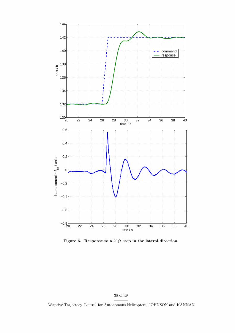
Finally, the controller was flight tested on the GTMax helicopter shown in Fig. 5. A lateral
position stepa response is shown in Fig. 6. The vehicle heading was regulated due-north
during this maneuver. Lateral control deflections during the maneuver were recorded and is
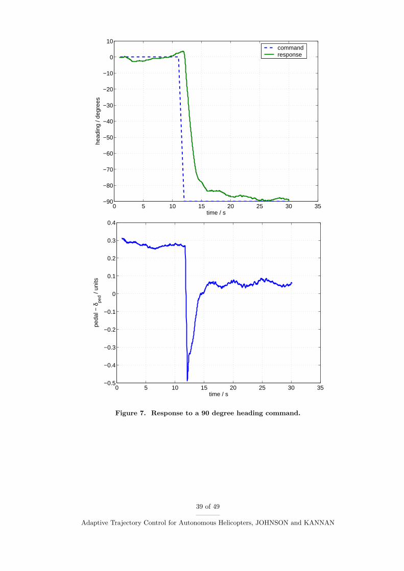
also shown. A step heading command response and pedal control history is shown in Fig. 7.
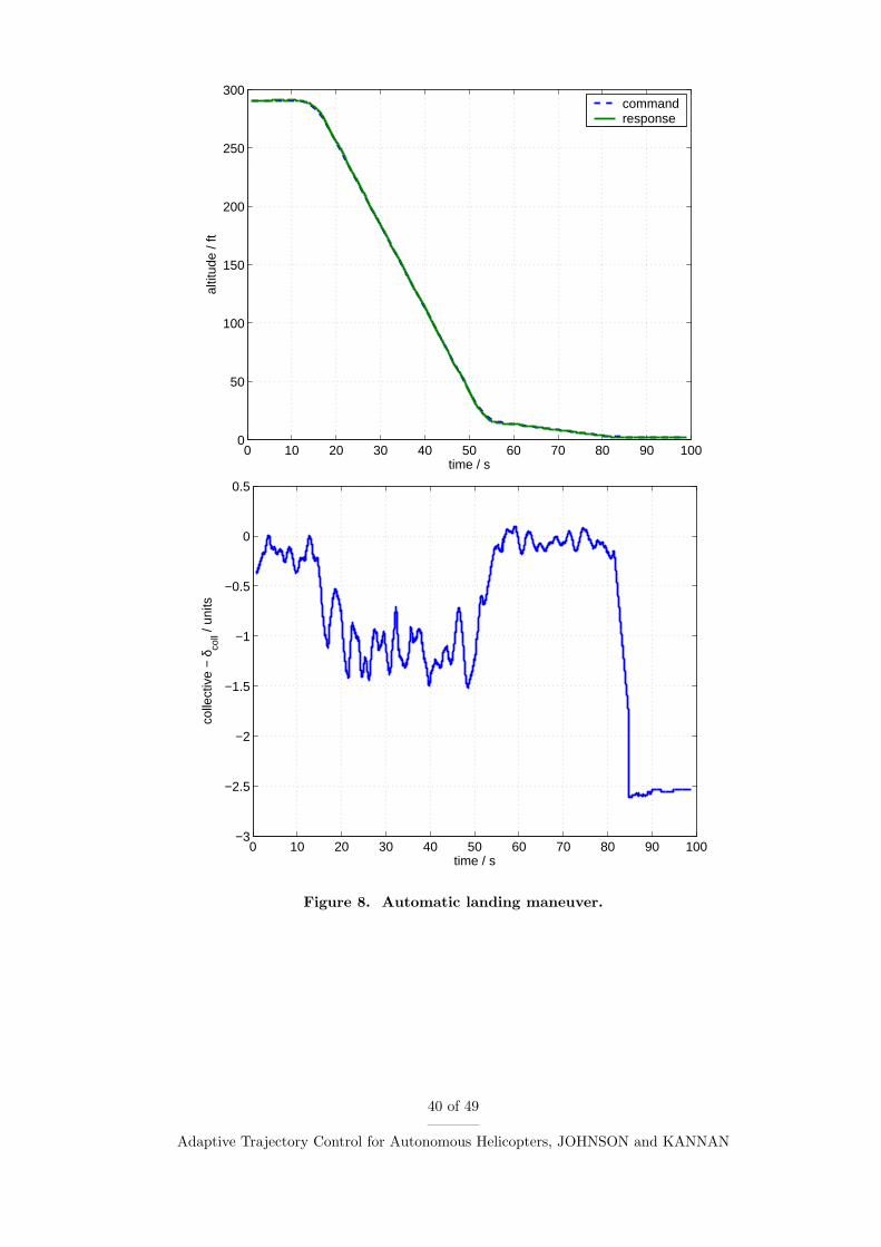
During takeoff and landing phases a range sensor (sonar) is used to maintain and update
the estimated local terrain altitude in the navigation system. The sonar is valid up to 8ft
above the terrain, sufficient for landing and takeoff purposes. Fig. 8 illustrates the altitude
and collective profile during a landing. The vehicle starts at an initial hover at 300ft,
followed by a descent at 7ft/s until the vehicle is 15ft above the estimated terrain. The
vehicle then descends at 0.5ft/s until weight-on-skids is automatically detected at which
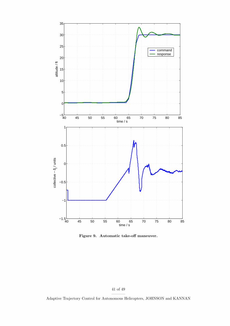
point the collective is slowly ramped down. Automatic takeoff (Fig. 9) is similar where the
collective is slowly ramped up until weight-on-skids is no longer detected. It should be noted
aDuring flight tests, variables were sampled at varying rates in order to conserve memory and datalinkbandwidth. The trajectory commands pc, vc, qc, ωc were sampled at 1Hz, actuator deflections δcoll, δlon, δlat
and δped were sampled at 50Hz, vehicle position and speed was sampled at 50Hz. Since the command vectoris sampled at a low rate (1Hz), a step command appears as a fast ramp in figures.
23 of 49
Adaptive Trajectory Control for Autonomous Helicopters, JOHNSON and KANNAN
that NN adaptation is active all times except when weight-on-skids is active. Additionally,
when weight is on skids, the collective ramp-up during takeoff and ramp-down during landing
is open-loop.
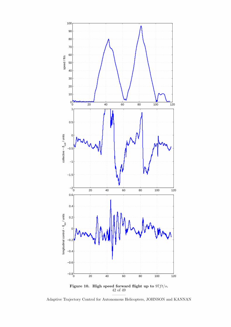
The approximate model used to compute the dynamic inverse (Eq. (63) and Eq. (60))
is based on a linear model of the dynamics in hover. To evaluate controller performance
at different points of the envelope, the vehicle was commanded to track a trajectory that
accelerated up to a speed of 100ft/s. To account for wind, an upwind and downwind leg
were flown. In the upwind leg the vehicle accelerated up to 80ft/s and during the backward
leg the vehicle accelerated up to a speed of 97ft/s as shown in Fig. 10. Collective and
longitudinal control deflections are also shown. In the upwind leg, the collective is saturated
and the vehicle is unable to accelerate further. The longitudinal control deflections behave
nominally as the vehicle accelerates and decelerates through a wide range of the envelope.
The NN is able to adapt to rapidly changing flight conditions, from the baseline inverting
design at hover through to the maximum speed of the aircraft. A conventional proportional-
integral-derivative design would have required scheduling of gains throughout the speed
range. More significantly, classical design would require accurate models at each point,
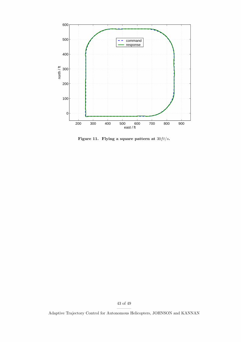
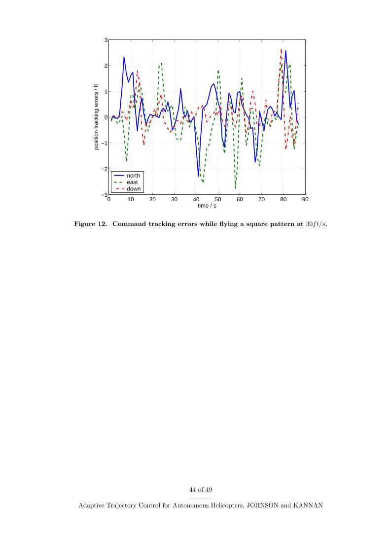
which our design does not. In addition to flight at high speeds, tracking performance was
evaluated at moderate speeds, where a square pattern was flown at 30ft/s for which position
tracking is shown in Fig. 11. External command position tracking errors are shown in Fig. 12
with a peak total position error 3.3ft and standard deviation of 0.8ft.
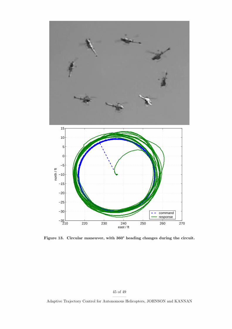
Many maneuvers such as high-speed flight are quasi steady, in the sense that once in
the maneuver, control deflection changes are only necessary for disturbance rejection. To
evaluate performance where the controls have to vary significantly in order to track the
commanded trajectory, the helicopter was commanded to perform a circular maneuver in the
north-east plane with constant altitude and a constantly changing heading. The trajectory
equations for this maneuver are given by
pc =
Vω
cos(ωt)
Vω
sin(ωt)
−h
, vc=
−V sin(ωt)
V cos(ωt)
0
ψc = ωtf (86)
where, t is current time and h is a constant altitude command. V is speed of the maneuver,
ω is angular speed of the helicopter around the maneuver origin, and f is number of 360°changes in heading to be performed per circuit. If ω = π/2rad/s, the helicopter will complete
the circular circuit once every 4 seconds. If f = 1, the helicopter will rotate anticlockwise
360° once per circuit. Fig. 13 shows the response to such a trajectory with parameters
24 of 49
Adaptive Trajectory Control for Autonomous Helicopters, JOHNSON and KANNAN
ω = 0.5rad/s, f = 1, V = 10ft/s. After the initial transition into the circular maneuver,
the tracking is seen to be within 5 ft. To visualize the maneuver easily, superimposed
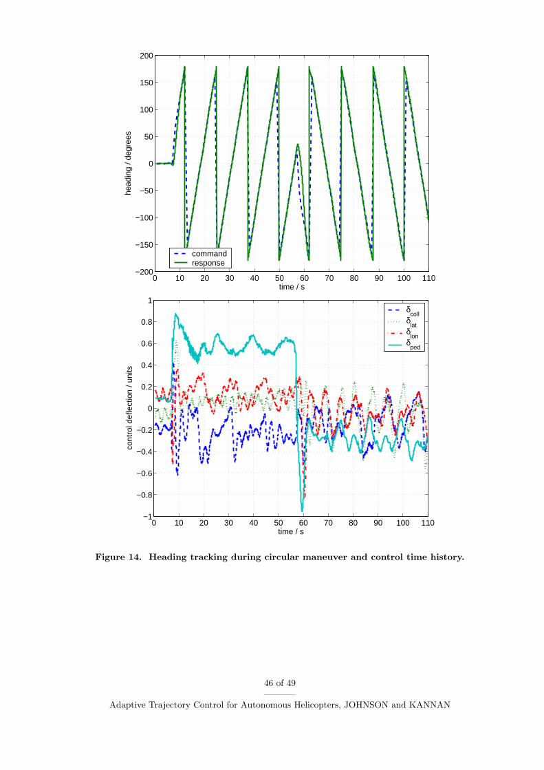
still images of the vehicle during the circular maneuver are shown. Both anticlockwise and
clockwise heading changes during the maneuver were tested by changing the parameter from
f = 1 (anticlockwise) to f = −1 (clockwise) at t = 55s. Fig. 14 shows that heading tracking
is good in both cases. The time history of the pedal input δped and all other controls during
the maneuver is also shown and illustrates how the vehicle has to exercise all of its controls
during this maneuver.
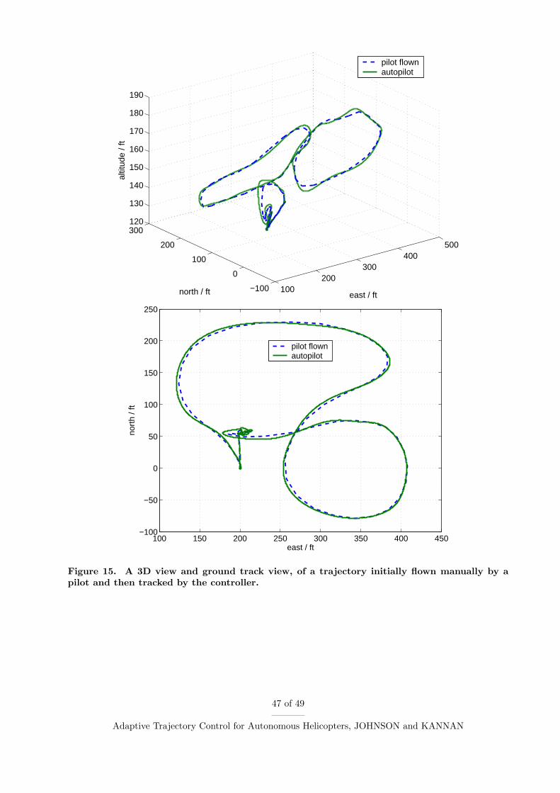
Next, the ability of the controller to track a previous manually-flown maneuver was tested.
First, a human pilot flew a figure eight, 3-dimensional pattern with the vehicle. Vehicle state
was recorded and was then played back as commands to the adaptive controller. A 3D plot of
the pilot and controller flown trajectories are shown in Fig. 15 along with projected ground
track. Overall, the tracking in position was measured to be within 11.3ft of the desired pilot
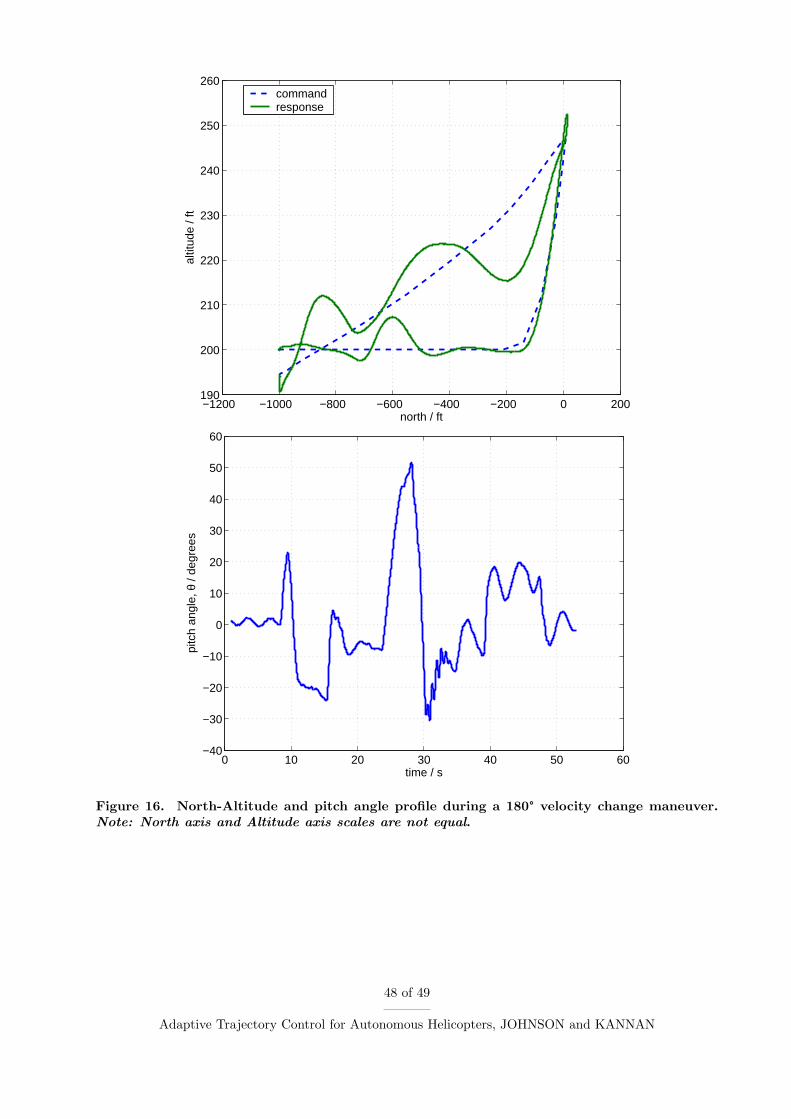
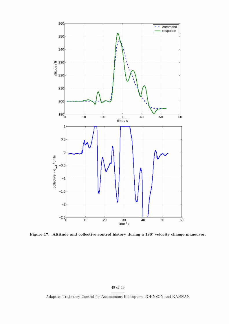
flown trajectory with a standard deviation of 4.7ft. Finally, a tactically useful maneuver was
flown to test controller performance at high speeds and pitch attitudes. The objective of the
maneuver is to make a 180-degree velocity change from a forward flight condition of 70ft/s
north to a 70ft/s forward flight going south. The trajectory command and response in the
north-altitude plane is shown in Fig. 16 along with the pitch angle. A time history of the
altitude and the collective control deflection is shown in Fig. 17. During the maneuver the
helicopter is commanded to increase altitude by up to 50ft in order to minimize saturation
of the down collective. In the deceleration phase the vehicle is able to track the command
trajectory well; however in accelerating to 70ft/s going south, tracking performance suffers.
In both the acceleration and deceleration phases, poor tracking corresponds with saturation
of the collective control. The oscillations in altitude in Fig. 17 are because the vehicle is
unable to maintain a lower descent rate due to saturation and is expected. The large pitch
attitudes experienced is what the outer-loop inversion evaluates as being required to perform
such rapid decelerations and accelerations. This experiment is an example of maneuvering
where the commanded trajectory is much more aggressive than the capability of the vehicle
and is reflected by the extended periods of saturation. It is possible to operate at the limits
of the vehicle primarily due to PCH which protects the adaptation process.
VII. Conclusions
The adaptive controller developed in this paper is able to correct for modeling errors
in both the attitude dynamics as well as the translation dynamics. Using PCH in a novel
way allows the outer loop to continue adapting correctly irrespective of the closed loop at-
titude dynamics or any limits inserted into the inner-loop reference model. A consolidated
25 of 49
Adaptive Trajectory Control for Autonomous Helicopters, JOHNSON and KANNAN
external command consisting of position, velocity, attitude and angular velocity may now
be provided to the control system. If the commanded trajectory is not feasible, causing
actuator saturation, the controller continues to operate at the actuator limits without af-
fecting adaptation. Additionally, expressions for the poles of the combined inner-outer-loop
error dynamics alleviates frequency separation requirements between the inner and outer
loops, allowing a higher outer-loop bandwidth, leading to better overall trajectory tracking
performance. Flight-test results over various ranges of the flight envelope illustrate that
adaptation may be used to successfully correct for significant model error arising from very
poor approximate models, in this case, a point mass model for translational dynamics and
a linear hover attitude dynamics model. Tracking error is small except in situations where
the actuators are saturated.
The control design presented here does not contain assumptions, that limit its application
to small unmanned helicopters. Desired response characteristics may be incorporated into
the design.
A. Appendix : Proof of Theorem 1
Proof. In the following proof a ’*’ represents ideal values, where the following variables,
W , W ∗ − W, V , V ∗ − V, z = V T x, z = z∗ − z hold. The arguments to the sigmoidal
activation function σ(·) are dropped for clarity and conciseness. Noting that the sigmoidal
functions are bounded, the NN output may be bounded as
νad = W T σ(z)
= (W ∗T − W T )σ(V T x)
‖νad‖ ≤ α0(Z + ‖Z‖F )
(87)
for some constant α0. This allows the inputs to the network to be bounded
x =[bv xT
c eTr eT νT
ad ‖Z‖F
]
‖x‖ ≤ bv + xc + er + ‖e‖+ α0(Z + ‖Z‖F ) + Z + ‖Z‖F
= k0 + k1‖Z‖F + ‖e‖(88)
where k1 = (1 + α0), k0 , bv + xc + er + k1Z. An expansion of σ(z) around the estimated
weights is given by
σ(z∗) = σ(z) +∂σ(s)
∂s
∣∣∣∣s=z
(z∗ − z) +O2(z) (89)
26 of 49
Adaptive Trajectory Control for Autonomous Helicopters, JOHNSON and KANNAN
Noting that the derivative of the sigmoidal function, σ′, is bounded, the higher order terms
of this expansion may be bounded as follows
O2(z) = σ(z∗)− σ(z)− σ′z
‖O2(z)‖ ≤ 2α0 + α1‖V T‖F‖x‖≤ 2α0 + α1k0‖Z‖F + α1k1‖Z‖2
F + α1‖Z‖F‖bfe‖(90)
By the substitution of νad = νad + νr, and ∆ = ∆ + εg = ν∗ad + ε + εg, the error dynamics
in Eq. (24) may be expressed as
e = Ae + B[νad − (ν∗ad + ε + εg) + νr] (91)
Now,
ν∗ad + ε + εg − νad = W ∗T σ∗ −W T σ + ε + εg
= W ∗T [σ(z) + σ′z +O2(z)
]−W T σ + ε + εg
adding and subtracting W T σ′z and W T σ′z∗
ν∗ad + ε + εg − νad = W T (σ − σ′z) + W T σ′z + w (92)
where,
w = W T σ′z∗ + W ∗TO2(z) + ε + εg (93)
the tracking error dynamics may finally be written as
e = Ae + B{−
[W T (σ − σ′z) + W T σ′z + w
]+ νr
}(94)
When the bounds computed earlier are used, the disturbance term w may be bounded as
‖w‖ = c0 + c1‖Z‖F + c2‖e‖‖Z‖F + c3‖Z‖2F (95)
where, c0, c1, c2, c3 are computable constants given by
c0 = 2α0Z + ε + εg
c1 = 2α1k0Z
c2 = 2α1k1Z
c3 = 2α1Z
(96)
27 of 49
Adaptive Trajectory Control for Autonomous Helicopters, JOHNSON and KANNAN
A Lyapunov candidate function is
L(e, W , V ) =1
2
[eT Pe + tr
(WΓ−1
W W T)
+ tr(V T Γ−1
V V)]
(97)
When the weight update equations of Eq. (58) and Eq. (59) are used, the time derivative of
L along trajectories can be expressed as
L = −1
2eT Qe + rT (−w + νr) + κ‖e‖tr
(ZT Z
)(98)
When Z = Z∗ − Z and ‖Z‖F ≥ ‖Z‖F − Z are used along with the robustifying term of
Eq. (57) and it is required that λmin(Kr) > c2, κ > ‖PB‖c3, L may be bounded as
L ≤ −1
2eT Qe + ‖r‖‖w‖ − rT Krr(‖Z‖F + Z)
‖e‖‖r‖ + κZ‖e‖‖Z‖F − κ‖e‖‖Z‖2
F (99)
L ≤ −1
2λmin(Q)‖e‖2 + ‖r‖‖w‖ − λmin(Kr)‖Z‖F‖e‖‖r‖+ κZ‖e‖‖Z‖F − κ‖e‖‖Z‖2
F
(100)
L ≤ −1
2λmin(Q)‖e‖2 + c0‖PB‖‖e‖+
(‖PB‖c1 + κZ) ‖e‖‖Z‖F
− (λmin(Kr)− c2)‖e‖‖r‖‖Z‖F − (κ− ‖PB‖c3) ‖e‖‖Z‖2F
(101)
L ≤ −1
2λmin(Q)‖e‖2 − (κ− ‖PB‖c3) ‖e‖‖Z‖2
F + a0‖e‖+ a1‖e‖‖Z‖F (102)
where,
a0 , c0‖PB‖a1 ,
(‖PB‖c1 + κZ)
(103)
By selecting λmin(Q), κ and learning rates (ΓW and ΓV ), L ≤ 0 everywhere outside a compact
set that is entirely within the largest level set of L, which in turn lies entirely within the
compact set D.15 It can be shown that L ≤ 0 when
‖Z‖F ≥ Zm =a1 +
√a2
1 + 4a0(κ− ‖PB‖c3)
2(κ− ‖PB‖c3)(104)
or
‖e‖ ≥ a0 + a1Zm
12λmin(Q)
(105)
28 of 49
Adaptive Trajectory Control for Autonomous Helicopters, JOHNSON and KANNAN
Thus for initial conditions within D, the tracking error e, and neural network weights W , V
are uniformly ultimately bounded,29 with the tracking error bound given by Eq. (105) treated
as an equality.
B. Acknowledgements
This work was supported in part by the Defense Advanced Research Projects Agency’s
Software Enabled Control Program under contracts #33615-98-C-1341 and #33615-99-C-
1500 with John S. Bay as program manager, William Koenig of the Air Force Research
Laboratory (AFRL) as Contract Monitor and in part by AFRL Contract #F33615-00-C-
3021. We also acknowledge the contributions of Aaron Kahn, Adrian Koller, J. Eric Corban,
Henrik Christophersen, Joerg Diettrich, Jeong Hur, Wayne Pickell and Alison Proctor and
who made the flight tests possible.
References
1Frazzoli, E., Dahleh, M. A., and Feron, E., “Real-Time Motion Planning for Agile
Autonomous Vehicles,” AIAA Journal of Guidance, Control, and Dynamics , Vol. 25, No. 1,
2002, pp. 116–129.
2Sanders, C. P., DeBitetto, P. D., Feron, E., Vuong, H. F., and Levenson, N., “Hierar-
chical Control of Small Autonomous Helicopters,” 37th IEEE Conference on Decision and
Control , Vol. 4, Tampa, Florida, December 1998.
3Gavrilets, V., Mettler, B., and Feron, E., “Nonlinear Model for a Small-Sized Acrobatic
Helicopter,” AIAA Guidance, Navigation and Control Conference, No. 2001-4333, Montreal,
Quebec, Canada, Aug. 2001.
4La Civita, M., Messner, W. C., and Kanade, T., “Modeling of Small-Scale Helicopters
with Integrated First-Principles and System-Identification Techniques,” Proceedings of the
58th Forum of the American Helicopter Society , Vol. 2, Montreal, Canada, June 2002, pp.
2505–2516.
5Mettler, B., Identification Modeling and Characteristics of Miniature Rotorcraft ,
Kluwer Academic Publishers, 2002.
6La Civita, M., Papageorgiou, G., Messner, W. C., and Kanade, T., “Design and Flight
Testing of a High Bandwidth H∞ Loop Shaping Controller for a Robotic Helicopter,” AIAA
Guidance, Navigation and Control Conference, No. AIAA-2002-4846, Monterey, CA, August
2002.
7Gavrilets, V., Mettler, B., and Feron, E., “Control Logic for Automated Aerobatic
Flight of Miniature Helicopter,” AIAA Guidance, Navigation and Control Conference, No.
29 of 49
Adaptive Trajectory Control for Autonomous Helicopters, JOHNSON and KANNAN
AIAA-2002-4834, Monterey, CA, August 2002.
8La Civita, M., Papageorgiou, G., Messner, W. C., and Kanade, T., “Design and Flight
Testing of a Gain-Scheduled H∞ Loop Shaping Controller for Wide-Envelope Flight of a
Robotic Helicopter,” Proceedings of the 2003 American Control Conference, Denver, CO,
June 2003, pp. 4195–4200.
9Calise, A. J., Lee, S., and Sharma, M., “Development of a Reconfigurable Flight Control
Law for Tailless Aircraft,” AIAA Journal of Guidance, Control, and Dynamics , Vol. 24,
No. 5, 2001, pp. 896–902.
10Brinker, J. and Wise, K., “Flight testing of a reconfigurable flight control law on the
X-36 tailless fighter aircraft,” AIAA Journal of Guidance, Control, and Dynamics , Vol. 24,
No. 5, 2001, pp. 903–909.
11Johnson, E. N. and Calise, A. J., “Limited Authority Adaptive Flight Control for
Reusable Launch Vehicles,” AIAA Journal of Guidance, Control, and Dynamics , Vol. 26,
No. 6, Nov-Dec 2003, pp. 906–913.
12Kim, N., Calise, A. J., Hovakimyan, N., Prasad, J., and Corban, J. E., “Adaptive
Output Feedback for High-Bandwidth Flight Control,” AIAA Journal of Guidance, Control,
and Dynamics , Vol. 25, No. 6, 2002, pp. 993–1002.
13Leitner, J., Calise, A. J., and Prasad, J. V. R., “Analysis of Adaptive Neural Networks
for Helicopter Flight Controls,” AIAA Journal of Guidance, Control, and Dynamics , Vol. 20,
No. 5, Sep-Oct 1997, pp. 972–979.
14Rysdyk, R. T. and Calise, A. J., “Adaptive Model Inversion Flight Control for Tiltrotor
Aircraft,” AIAA Journal of Guidance, Control, and Dynamics , Vol. 22, No. 3, 1999, pp. 402–
407.
15Johnson, E. N., Limited Authority Adaptive Flight Control , Ph.D. thesis, Georgia In-
stitute of Technology, School of Aerospace Engineering, Atlanta, GA 30332, Dec 2000.
16Rysdyk, R. T. and Calise, A. J., “Nonlinear Adaptive Flight Control Using Neural
Networks,” IEEE Controls Systems Magazine, Vol. 18, No. 6, Dec 1998, pp. 14–25.
17Stevens, B. L. and Lewis, F. L., Aircraft Control and Simulaion, John Wiley & Sons,
New York, 2003.
18Johnson, E. N. and Kannan, S. K., “Nested Saturation with Guaranteed Real Poles,”
American Control Conference, Vol. 1, Boulder, Colorado, June 2003, pp. 497–502.
19Kannan, S. K. and Johnson, E. N., “Adaptive Control with a Nested Saturation Ref-
erence Model,” AIAA Guidance, Navigation and Control Conference, No. AIAA-2003-5324,
Austin, TX, August 2003.
20Hornik, K., Stinchcombe, M., and White, H., “Multilayer feedforward networks are
universal approximators,” Neural Networks , Vol. 2, No. 5, 1989, pp. 359–366.
30 of 49
Adaptive Trajectory Control for Autonomous Helicopters, JOHNSON and KANNAN
21Spooner, J. T., Maggiore, M., Ordonez, R., and Passino, K. M., Stable Adaptive Control
and Estimation for Nonlinear Systems, Neural and Fuzzy Approximator Techniques , Wiley,
2002.
22Lewis, F. L., “Nonlinear Network Structures for Feedback Control (Survey Paper),”
Asian Journal of Control , Vol. 1, No. 4, 1999, pp. 205–228.
23Calise, A. J., Hovakimyan, N., and Idan, M., “Adaptive Output Feedback Control of
Nonlinear Systems Using Neural Networks,” Automatica, Vol. 37, No. 8, aug 2001, pp. 1201–
1211, Special Issue on Neural Networks for Feedback Control.
24Munzinger, C., Development of a Real-Time Flight Simulator for An Experimental
Model Helicopter , Master’s thesis, Georgia Institute of Technology, School of Aerospace
Engineering, Atlanta, GA 30332, Jul 1997.
25Lipp, A. M. and Prasad, J. V. R., “Synthesis of a Helicopter Nonlinear Flight Controller
Using Approximate Model Inversion,” Mathematical and Computer Modelling , Vol. 18, Au-
gust 1993, pp. 89–100.
26Aeronautical Design Standard, Handling Qualities Requirements for Military Rotor-
craft, ADS-33E , United States Army Aviation and Missile Command, Redstone Arsenal,
Alabama, March 2000.
27Johnson, E. N. and Kannan, S. K., “Adaptive Flight Control for an Autonomous Un-
manned Helicopter,” AIAA Guidance, Navigation and Control Conference, No. AIAA-2002-
4439, Monterey, CA, August 2002.
28Johnson, E. N. and Schrage, D. P., “System Integration and Operation of a Research
Unmanned Aerial Vehicle,” AIAA Journal of Aerospace Computing, Information and Com-
munication, Vol. 1, No. 1, Jan 2004, pp. 5–18.
29Narendra, K. S. and Annaswamy, A. M., “A New Adaptive Law for Robust Adaptation
Without Persistent Excitation,” IEEE Transactions on Automatic Control , Vol. 32, No. 2,
Februrary 1987, pp. 134–145.
31 of 49
Adaptive Trajectory Control for Autonomous Helicopters, JOHNSON and KANNAN
List of Figures
1 Overall Inner and Outerloop with Adaptation and Hedging. . . . . . . . . . 332 Neural Network with one hidden layer. . . . . . . . . . . . . . . . . . . . . . 343 Point mass model for outerloop inversion. . . . . . . . . . . . . . . . . . . . . 354 Detailed inner and outer loop controller architecture for an autonomous heli-
copter. . . . . . . . . . . . . . . . . . . . . . . . . . . . . . . . . . . . . . . . 365 The GTMax Helicopter. . . . . . . . . . . . . . . . . . . . . . . . . . . . . . 376 Response to a 20ft step in the lateral direction. . . . . . . . . . . . . . . . . 387 Response to a 90 degree heading command. . . . . . . . . . . . . . . . . . . 398 Automatic landing maneuver. . . . . . . . . . . . . . . . . . . . . . . . . . . 409 Automatic take-off maneuver. . . . . . . . . . . . . . . . . . . . . . . . . . . 4110 High speed forward flight up to 97ft/s. . . . . . . . . . . . . . . . . . . . . . 4211 Flying a square pattern at 30ft/s. . . . . . . . . . . . . . . . . . . . . . . . . 4312 Command tracking errors while flying a square pattern at 30ft/s. . . . . . . 4413 Circular maneuver, with 360° heading changes during the circuit. . . . . . . 4514 Heading tracking during circular maneuver and control time history. . . . . . 4615 A 3D view and ground track view, of a trajectory initially flown manually by
a pilot and then tracked by the controller. . . . . . . . . . . . . . . . . . . . 4716 North-Altitude and pitch angle profile during a 180° velocity change maneuver.
Note: North axis and Altitude axis scales are not equal. . . . . . . . . . . . . 4817 Altitude and collective control history during a 180° velocity change maneuver. 49
32 of 49
Adaptive Trajectory Control for Autonomous Helicopters, JOHNSON and KANNAN
Inner
Loop
Outer
Loopdesq
ccq w,
cc vp ,md
Outer Loop
Hedge
Inner Loop
Hedgeha ha
Adaptive
Elementax ˆ,ˆ,a
adaada
fd
xx xx
Figure 1. Overall Inner and Outerloop with Adaptation and Hedging.
33 of 49
Adaptive Trajectory Control for Autonomous Helicopters, JOHNSON and KANNAN
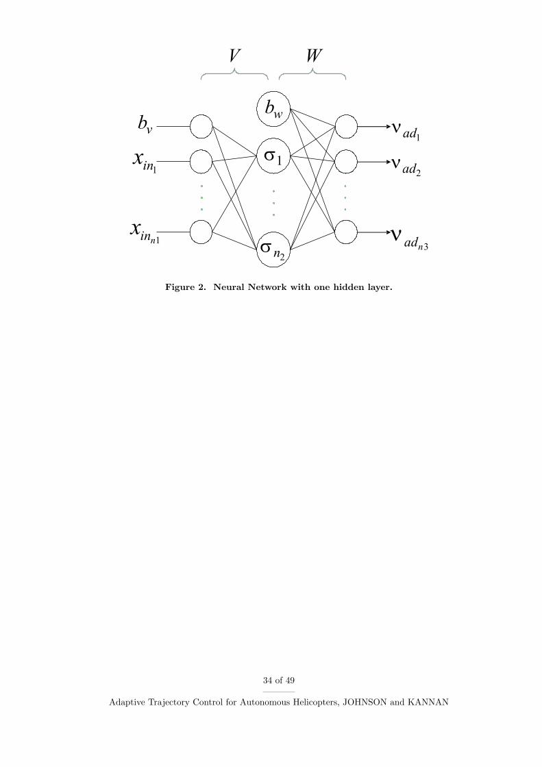
Figure 2. Neural Network with one hidden layer.
34 of 49
Adaptive Trajectory Control for Autonomous Helicopters, JOHNSON and KANNAN
1DF
initialBy
initialBz
)(3 initialBg
sff
2desa
finalBy
finalBz
Figure 3. Point mass model for outerloop inversion.
35 of 49
Adaptive Trajectory Control for Autonomous Helicopters, JOHNSON and KANNAN
NN
Inner
Loop
Appro
x
Inver
sion
Inner
-Loop
Hed
ge
Oute
r L
oop
Ref
eren
ce M
odel
Pla
nt
Oute
r-L
oop
Hed
ge
Oute
r-L
oop
PD
Inner
-Loop
PD
cr
a
rr
ww
,,
,r
rv
pv
p,
,,
w,,
,q
vp
aw
ˆ,ˆ
,,
,,
aq
vp
w,,
,q
vp
Inner
Loop
Ref
eren
ce M
odel
Oute
r L
oop
Appro
x
Inver
sion
cc
vp
,w,
,,
qv
p
w,,
,q
vp
w,,
,q
vp
des
q
des
coll
d
des
ped
lon
lat
],
,[
dd
d
cr
a
ad
a-
ad
a-
ha
ha
OU
TE
R L
OO
PIN
NE
R L
OO
P
cc
qw,
++
Figure 4. Detailed inner and outer loop controller architecture for an autonomous helicopter.
36 of 49
Adaptive Trajectory Control for Autonomous Helicopters, JOHNSON and KANNAN
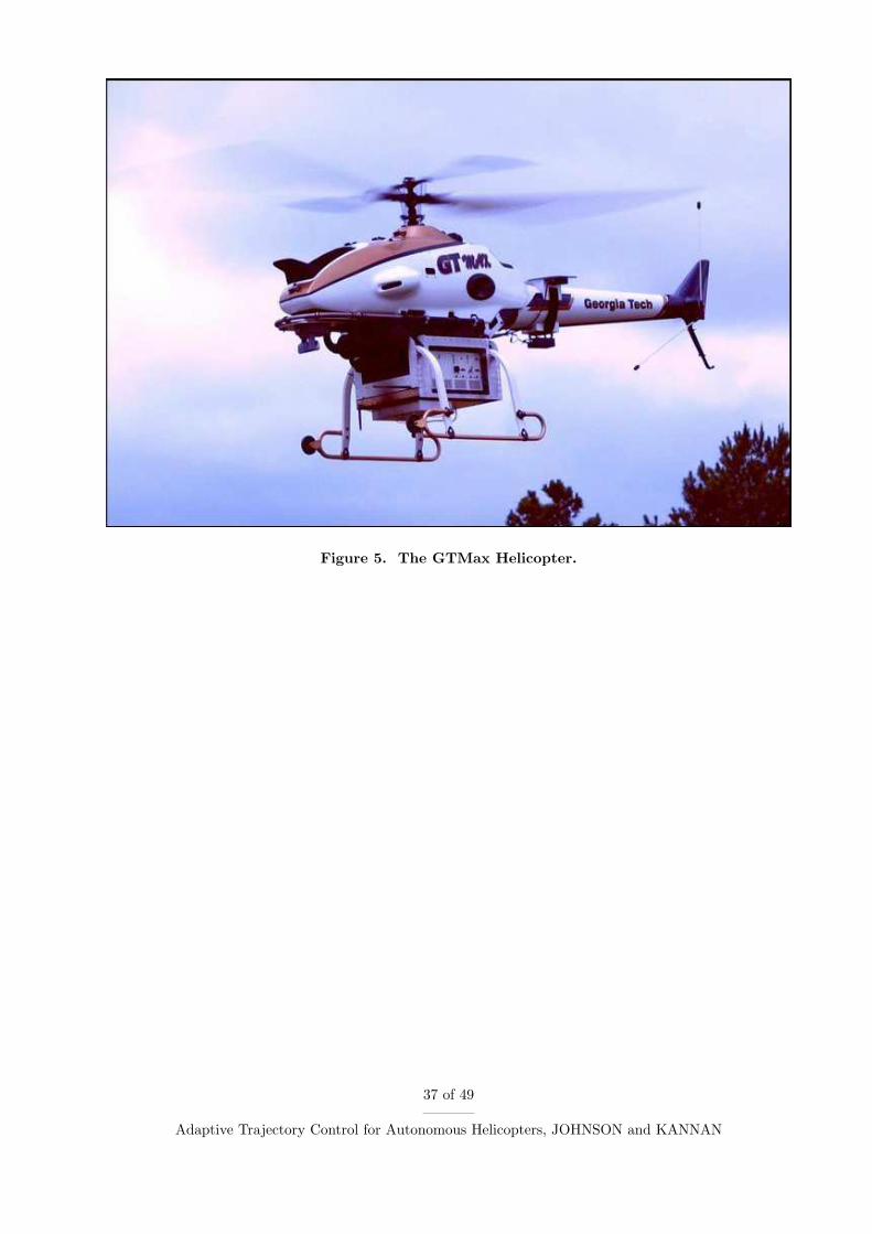
Figure 5. The GTMax Helicopter.
37 of 49
Adaptive Trajectory Control for Autonomous Helicopters, JOHNSON and KANNAN
20 22 24 26 28 30 32 34 36 38 40130
132
134
136
138
140
142
144
east
/ ft
time / s
commandresponse
20 22 24 26 28 30 32 34 36 38 40−0.8
−0.6
−0.4
−0.2
0
0.2
0.4
0.6
late
ral c
ontr
ol −
δla
t / un
its
time / s
Figure 6. Response to a 20ft step in the lateral direction.
38 of 49
Adaptive Trajectory Control for Autonomous Helicopters, JOHNSON and KANNAN
0 5 10 15 20 25 30 35−90
−80
−70
−60
−50
−40
−30
−20
−10
0
10
head
ing
/ deg
rees
time / s
commandresponse
0 5 10 15 20 25 30 35−0.5
−0.4
−0.3
−0.2
−0.1
0
0.1
0.2
0.3
0.4
peda
l − δ
ped /
units
time / s
Figure 7. Response to a 90 degree heading command.
39 of 49
Adaptive Trajectory Control for Autonomous Helicopters, JOHNSON and KANNAN
0 10 20 30 40 50 60 70 80 90 1000
50
100
150
200
250
300
altit
ude
/ ft
time / s
commandresponse
0 10 20 30 40 50 60 70 80 90 100−3
−2.5
−2
−1.5
−1
−0.5
0
0.5
colle
ctiv
e −
δco
ll / un
its
time / s
Figure 8. Automatic landing maneuver.
40 of 49
Adaptive Trajectory Control for Autonomous Helicopters, JOHNSON and KANNAN
40 45 50 55 60 65 70 75 80 85−5
0
5
10
15
20
25
30
35
altit
ude
/ ft
time / s
commandresponse
40 45 50 55 60 65 70 75 80 85−1.5
−1
−0.5
0
0.5
1
colle
ctiv
e −
δf /
units
time / s
Figure 9. Automatic take-off maneuver.
41 of 49
Adaptive Trajectory Control for Autonomous Helicopters, JOHNSON and KANNAN
0 20 40 60 80 100 1200
10
20
30
40
50
60
70
80
90
100
spee
d / f
t/s
0 20 40 60 80 100 120−2
−1.5
−1
−0.5
0
0.5
1
colle
ctiv
e −
δco
ll / un
its
0 20 40 60 80 100 120−0.8
−0.6
−0.4
−0.2
0
0.2
0.4
0.6
long
itudi
nal c
ontr
ol −
δlo
n / un
its
Figure 10. High speed forward flight up to 97ft/s.42 of 49
Adaptive Trajectory Control for Autonomous Helicopters, JOHNSON and KANNAN
200 300 400 500 600 700 800 900
0
100
200
300
400
500
600
nort
h / f
t
east / ft
commandresponse
Figure 11. Flying a square pattern at 30ft/s.
43 of 49
Adaptive Trajectory Control for Autonomous Helicopters, JOHNSON and KANNAN
0 10 20 30 40 50 60 70 80 90−3
−2
−1
0
1
2
3
posi
tion
trac
king
err
ors
/ ft
time / s
northeastdown
Figure 12. Command tracking errors while flying a square pattern at 30ft/s.
44 of 49
Adaptive Trajectory Control for Autonomous Helicopters, JOHNSON and KANNAN
210 220 230 240 250 260 270−35
−30
−25
−20
−15
−10
−5
0
5
10
15
nort
h / f
t
east / ft
commandresponse
Figure 13. Circular maneuver, with 360° heading changes during the circuit.
45 of 49
Adaptive Trajectory Control for Autonomous Helicopters, JOHNSON and KANNAN
0 10 20 30 40 50 60 70 80 90 100 110−200
−150
−100
−50
0
50
100
150
200
head
ing
/ deg
rees
time / s
commandresponse
0 10 20 30 40 50 60 70 80 90 100 110−1
−0.8
−0.6
−0.4
−0.2
0
0.2
0.4
0.6
0.8
1
cont
rol d
efle
ctio
n / u
nits
time / s
δcoll
δlat
δlon
δped
Figure 14. Heading tracking during circular maneuver and control time history.
46 of 49
Adaptive Trajectory Control for Autonomous Helicopters, JOHNSON and KANNAN
100200
300400
500
−100
0
100
200
300120
130
140
150
160
170
180
190
east / ftnorth / ft
altit
ude
/ ft
pilot flownautopilot
100 150 200 250 300 350 400 450−100
−50
0
50
100
150
200
250
nort
h / f
t
east / ft
pilot flownautopilot
Figure 15. A 3D view and ground track view, of a trajectory initially flown manually by apilot and then tracked by the controller.
47 of 49
Adaptive Trajectory Control for Autonomous Helicopters, JOHNSON and KANNAN
−1200 −1000 −800 −600 −400 −200 0 200190
200
210
220
230
240
250
260
north / ft
altit
ude
/ ft
commandresponse
0 10 20 30 40 50 60−40
−30
−20
−10
0
10
20
30
40
50
60
pitc
h an
gle,
θ /
degr
ees
time / s
Figure 16. North-Altitude and pitch angle profile during a 180° velocity change maneuver.Note: North axis and Altitude axis scales are not equal.
48 of 49
Adaptive Trajectory Control for Autonomous Helicopters, JOHNSON and KANNAN
0 10 20 30 40 50 60190
200
210
220
230
240
250
260
altit
ude
/ ft
time / s
commandresponse
0 10 20 30 40 50 60−2.5
−2
−1.5
−1
−0.5
0
0.5
1
colle
ctiv
e −
δco
ll / un
its
time / s
Figure 17. Altitude and collective control history during a 180° velocity change maneuver.
49 of 49
Adaptive Trajectory Control for Autonomous Helicopters, JOHNSON and KANNAN


