
1N. Gauger et al.Intro to Optimization and MDO, VKI, March 6-10,2006
Adjoint Approaches in Aerodynamic Shape Optimization and MDO Context I/II
Nicolas Gauger 1), 2)
1) DLR BraunschweigInstitute of Aerodynamics and Flow Technology
Numerical Methods Branch2) Humboldt University Berlin
Department of Mathematics
Introduction to Optimization and Multidisciplinary DesignVKI, March 6-10, 2006
http://www.mathematik.hu-berlin.de/~gauger
2N. Gauger et al.Intro to Optimization and MDO, VKI, March 6-10,2006
CollaboratorsWith contributions to this lecture:
• DLR: N. Kroll, J. Brezillon, A. Fazzolari,
R. Dwight, M. Widhalm
• HU Berlin: A. Griewank, J. Riehme
• Fastopt: R. Giering, Th. Kaminski
• TU Dresden: A. Walther, C. Moldenhauer
• Uni Trier: V. Schulz, S. HazraUniversity of Trier
FastOpt
3N. Gauger et al.Intro to Optimization and MDO, VKI, March 6-10,2006
Content of lecture
Why adjoint approaches?
What is an adjoint approach?
Continuous and discrete adjoint approaches / solvers
Validation and Application in 2D and 3D, Euler and Navier-Stokes
Algorithmic / Automated Differentiation (AD)
Coupled aero-structure adjoint approach
Validation and application in MDO context
One shot approaches
4N. Gauger et al.Intro to Optimization and MDO, VKI, March 6-10,2006
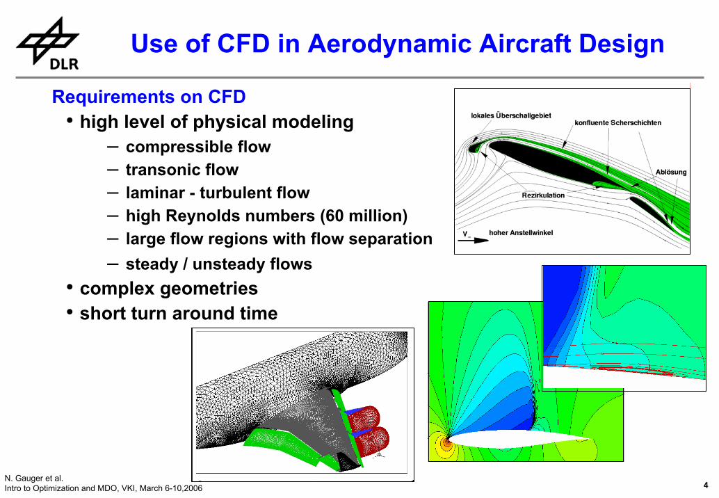
Requirements on CFD• high level of physical modeling
– compressible flow– transonic flow– laminar - turbulent flow – high Reynolds numbers (60 million)– large flow regions with flow separation – steady / unsteady flows
• complex geometries• short turn around time
Use of CFD in Aerodynamic Aircraft Design
5N. Gauger et al.Intro to Optimization and MDO, VKI, March 6-10,2006
Consequencessolution of 3D compressible Reynolds averaged Navier-Stokes equations turbulence models based on transport equations (2 – 6 eqn)models for predicting laminar-turbulent transition flexible grid generation techniques with high level of automation(block structured grids, overset grids, unstructured/hybrid grids)link to CAD-systemsefficient algorithms (multigrid, grid adaptation, parallel algorithms...)large scale computations ( ~ 10 - 25 million grid points)…
Use of CFD in Aerodynamic Aircraft Design
6N. Gauger et al.Intro to Optimization and MDO, VKI, March 6-10,2006
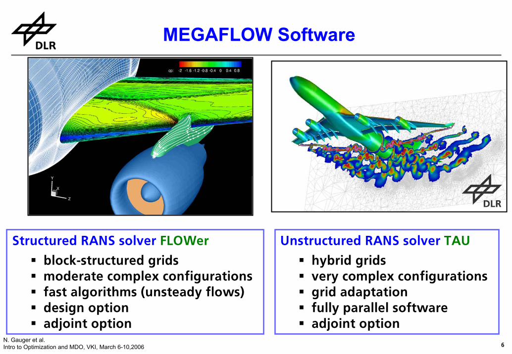
MEGAFLOW Software
Structured RANS solver FLOWer
block-structured grids moderate complex configurationsfast algorithms (unsteady flows)design optionadjoint option
Unstructured RANS solver TAU
hybrid grids very complex configurationsgrid adaptation fully parallel softwareadjoint option
7N. Gauger et al.Intro to Optimization and MDO, VKI, March 6-10,2006
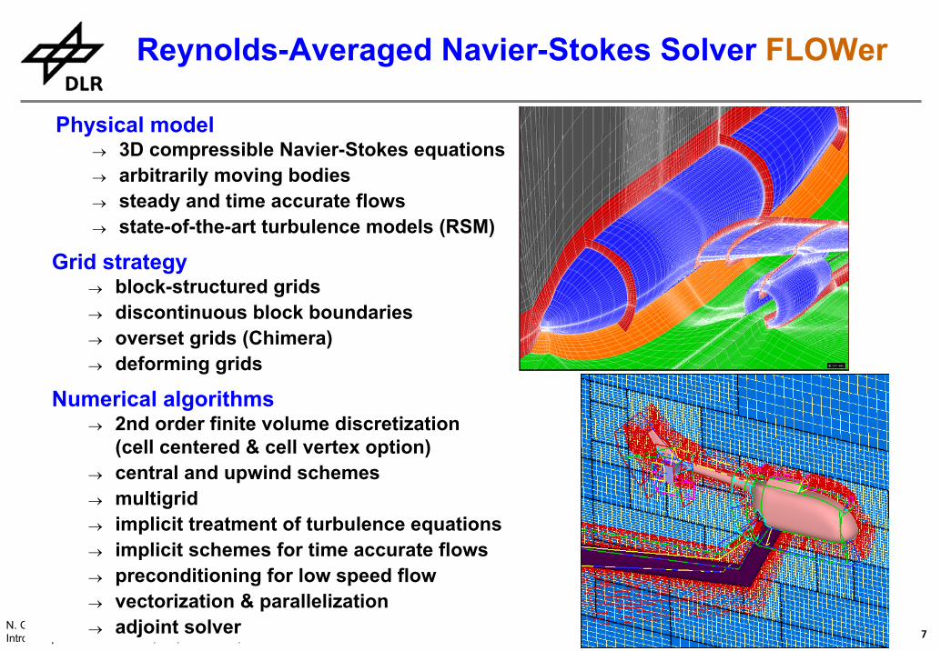
Physical model→ 3D compressible Navier-Stokes equations→ arbitrarily moving bodies→ steady and time accurate flows→ state-of-the-art turbulence models (RSM)
Reynolds-Averaged Navier-Stokes Solver FLOWer
Numerical algorithms→ 2nd order finite volume discretization
(cell centered & cell vertex option)→ central and upwind schemes→ multigrid→ implicit treatment of turbulence equations→ implicit schemes for time accurate flows→ preconditioning for low speed flow→ vectorization & parallelization→ adjoint solver
Grid strategy→ block-structured grids→ discontinuous block boundaries→ overset grids (Chimera)→ deforming grids
8N. Gauger et al.Intro to Optimization and MDO, VKI, March 6-10,2006
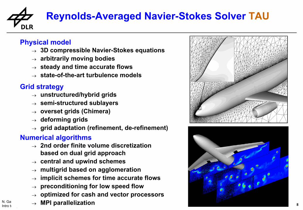
Physical model→ 3D compressible Navier-Stokes equations→ arbitrarily moving bodies→ steady and time accurate flows→ state-of-the-art turbulence models
Reynolds-Averaged Navier-Stokes Solver TAU
Numerical algorithms→ 2nd order finite volume discretization
based on dual grid approach→ central and upwind schemes→ multigrid based on agglomeration → implicit schemes for time accurate flows→ preconditioning for low speed flow→ optimized for cash and vector processors→ MPI parallelization
Grid strategy→ unstructured/hybrid grids→ semi-structured sublayers→ overset grids (Chimera)→ deforming grids → grid adaptation (refinement, de-refinement)
9N. Gauger et al.Intro to Optimization and MDO, VKI, March 6-10,2006
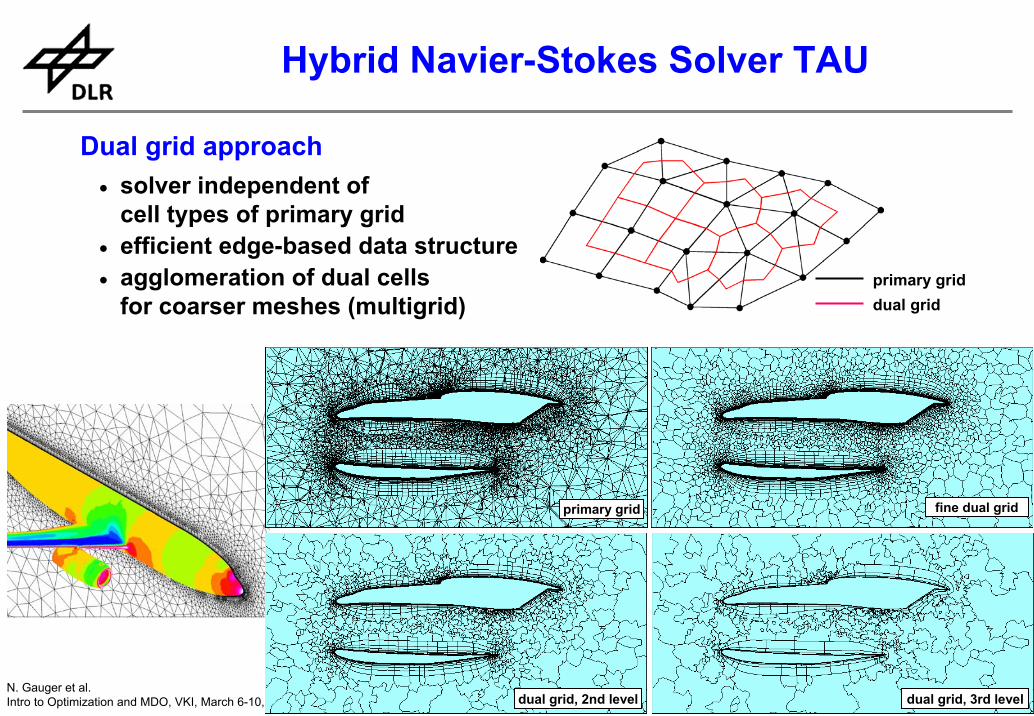
Dual grid approach• solver independent of
cell types of primary grid• efficient edge-based data structure• agglomeration of dual cells
for coarser meshes (multigrid)
Hybrid Navier-Stokes Solver TAU
primary grid fine dual grid
dual grid, 2nd level dual grid, 3rd level
primary griddual grid
10N. Gauger et al.Intro to Optimization and MDO, VKI, March 6-10,2006
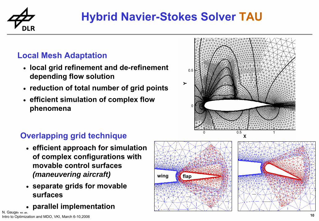
Hybrid Navier-Stokes Solver TAU
Local Mesh Adaptation• local grid refinement and de-refinement
depending flow solution • reduction of total number of grid points• efficient simulation of complex flow
phenomena
Overlapping grid technique• efficient approach for simulation
of complex configurations withmovable control surfaces (maneuvering aircraft)
• separate grids for movable surfaces
• parallel implementation
wing flap
11N. Gauger et al.Intro to Optimization and MDO, VKI, March 6-10,2006
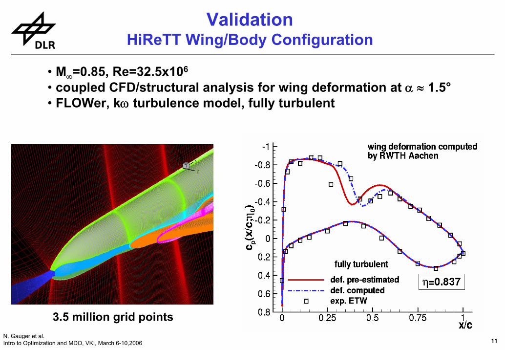
• M∞=0.85, Re=32.5x10⁶
• coupled CFD/structural analysis for wing deformation at α ≈ 1.5°• FLOWer, kω turbulence model, fully turbulent
ValidationHiReTT Wing/Body Configuration
3.5 million grid points
12N. Gauger et al.Intro to Optimization and MDO, VKI, March 6-10,2006
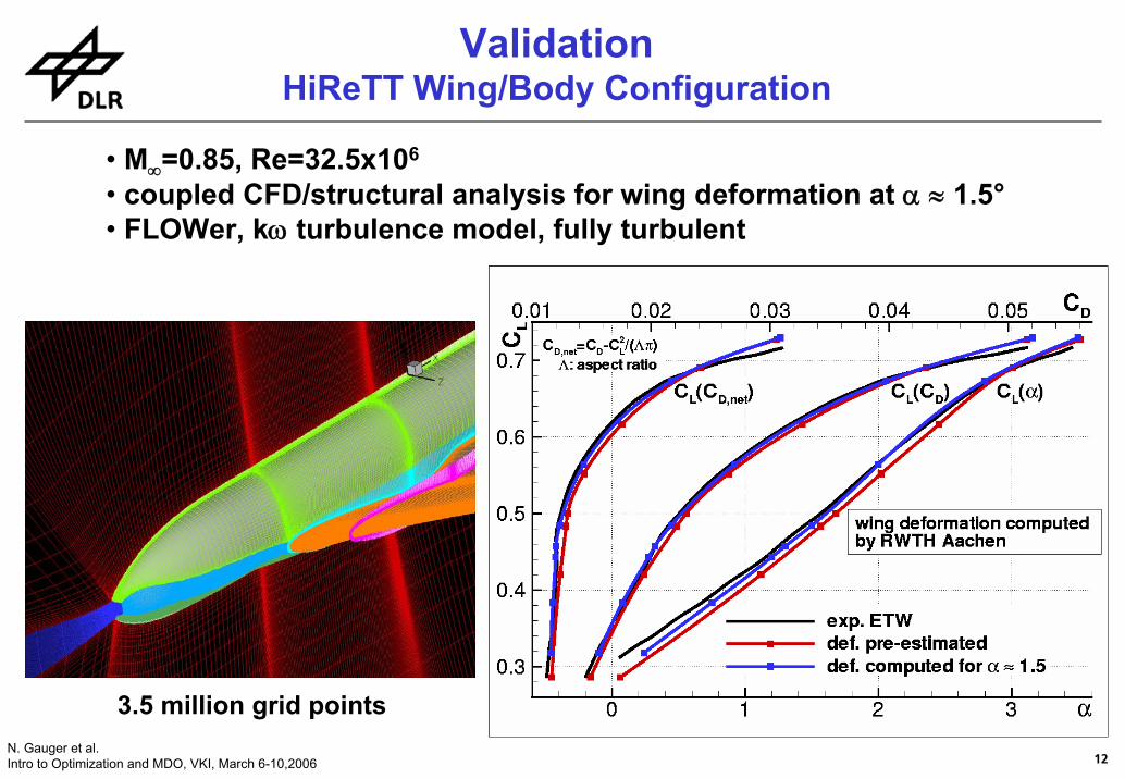
• M∞=0.85, Re=32.5x10⁶
• coupled CFD/structural analysis for wing deformation at α ≈ 1.5°• FLOWer, kω turbulence model, fully turbulent
ValidationHiReTT Wing/Body Configuration
3.5 million grid points
13N. Gauger et al.Intro to Optimization and MDO, VKI, March 6-10,2006
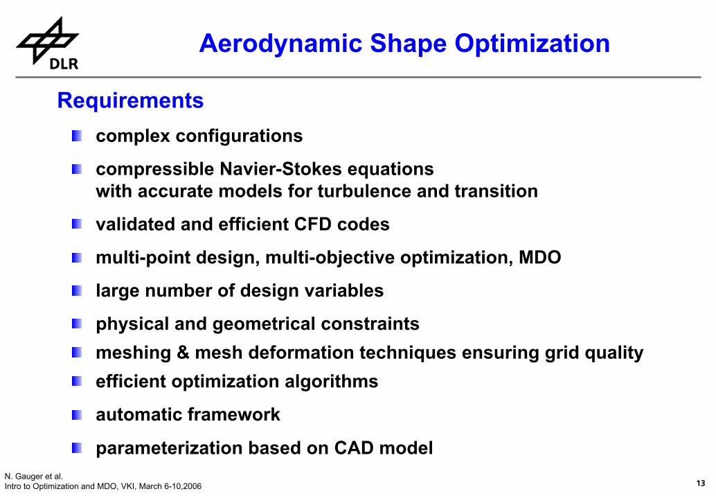
Requirementscomplex configurations
compressible Navier-Stokes equationswith accurate models for turbulence and transition
validated and efficient CFD codes
multi-point design, multi-objective optimization, MDO
large number of design variables
physical and geometrical constraintsmeshing & mesh deformation techniques ensuring grid qualityefficient optimization algorithms
automatic framework
parameterization based on CAD model
Aerodynamic Shape Optimization
14N. Gauger et al.Intro to Optimization and MDO, VKI, March 6-10,2006
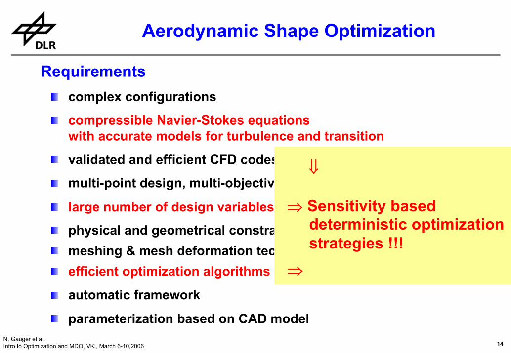
Requirementscomplex configurations
compressible Navier-Stokes equationswith accurate models for turbulence and transition
validated and efficient CFD codes
multi-point design, multi-objective optimization, MDO
large number of design variables
physical and geometrical constraintsmeshing & mesh deformation techniques ensuring grid qualityefficient optimization algorithms
automatic framework
parameterization based on CAD model
Aerodynamic Shape Optimization
⇓
⇒ Sensitivity baseddeterministic optimizationstrategies !!!
⇒
15N. Gauger et al.Intro to Optimization and MDO, VKI, March 6-10,2006
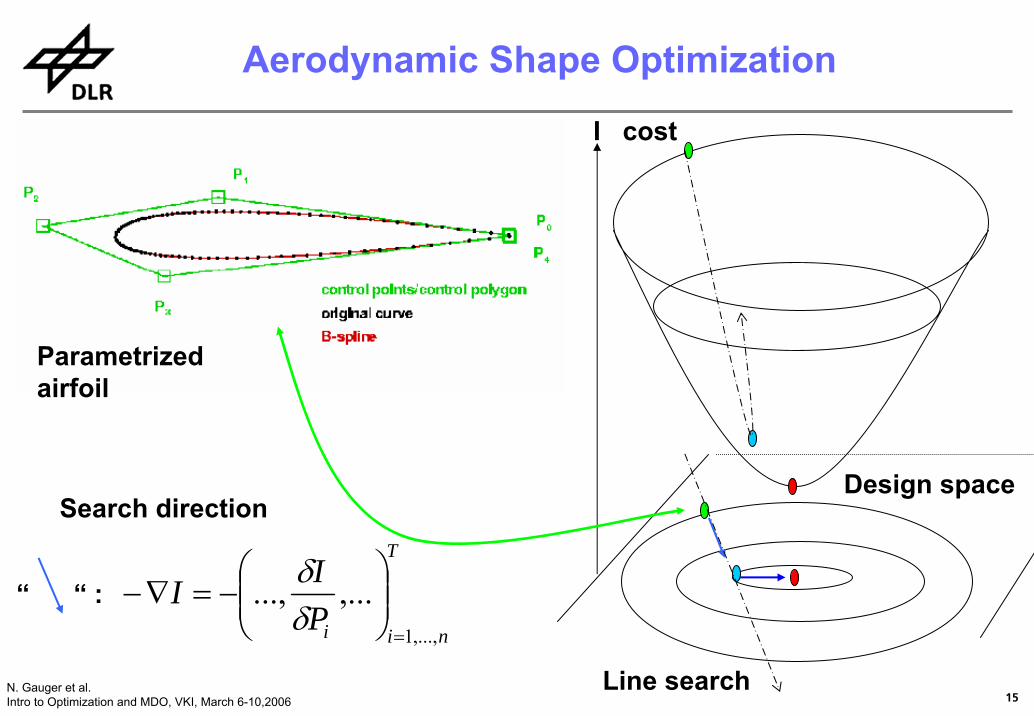
Parametrizedairfoil
Design space
I cost
T
niiPII
,...,1
,......,=
⎟⎟⎠
⎞⎜⎜⎝
⎛−=∇−
δδ
“ “ :
Line search
Search direction
Aerodynamic Shape Optimization
16N. Gauger et al.Intro to Optimization and MDO, VKI, March 6-10,2006
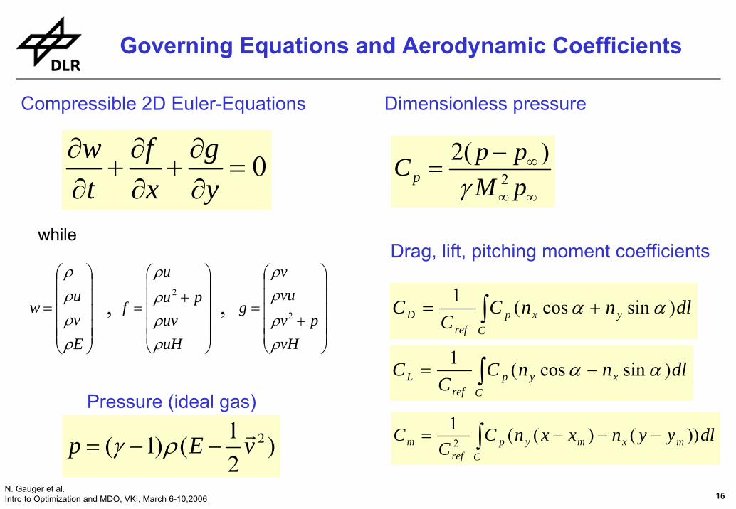
0=∂∂
+∂∂
+∂∂
yg
xf
tw
∞∞
∞−=
pMppCp 2
)(2γ
∫ +=C
yxpref
D dlnnCC
C )sincos(1 αα
∫ −=C
xypref
L dlnnCC
C )sincos(1 αα
∫ −−−=C
mxmypref
m dlyynxxnCC
C ))()((12
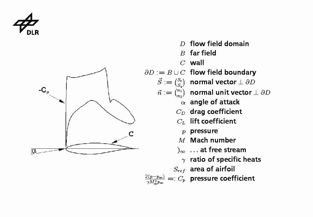
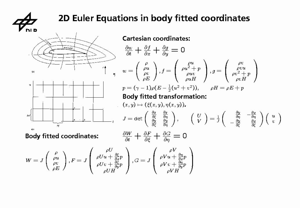
Compressible 2D Euler-Equations
while
⎟⎟⎟⎟⎟
⎠
⎞
⎜⎜⎜⎜⎜
⎝
⎛
+=
uHuv
puu
f
ρρρ
ρ2
⎟⎟⎟⎟⎟
⎠
⎞
⎜⎜⎜⎜⎜
⎝
⎛
+=
vHpv
vuv
g
ρρ
ρρ
2
⎟⎟⎟⎟⎟
⎠
⎞
⎜⎜⎜⎜⎜
⎝
⎛
=
Evu
w
ρρρρ
, ,
Dimensionless pressure
Drag, lift, pitching moment coefficients
Pressure (ideal gas)
)21()1( 2vEp r
−−= ργ
Governing Equations and Aerodynamic Coefficients
17N. Gauger et al.Intro to Optimization and MDO, VKI, March 6-10,2006
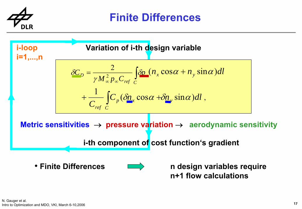
• Finite Differences n design variables requiren+1 flow calculations
Metric sensitivities → pressure variation → aerodynamic sensitivity
∫∞∞
=Cref
D pCpM
C δγ
δ 22 dlnn yx )sincos( αα +
dlnnCC y
Cxp
ref
)sincos(1 αδαδ∫ ++ ,
i-th component of cost function‘s gradient
i-loopi=1,...,n
Variation of i-th design variable
Finite Differences
18N. Gauger et al.Intro to Optimization and MDO, VKI, March 6-10,2006
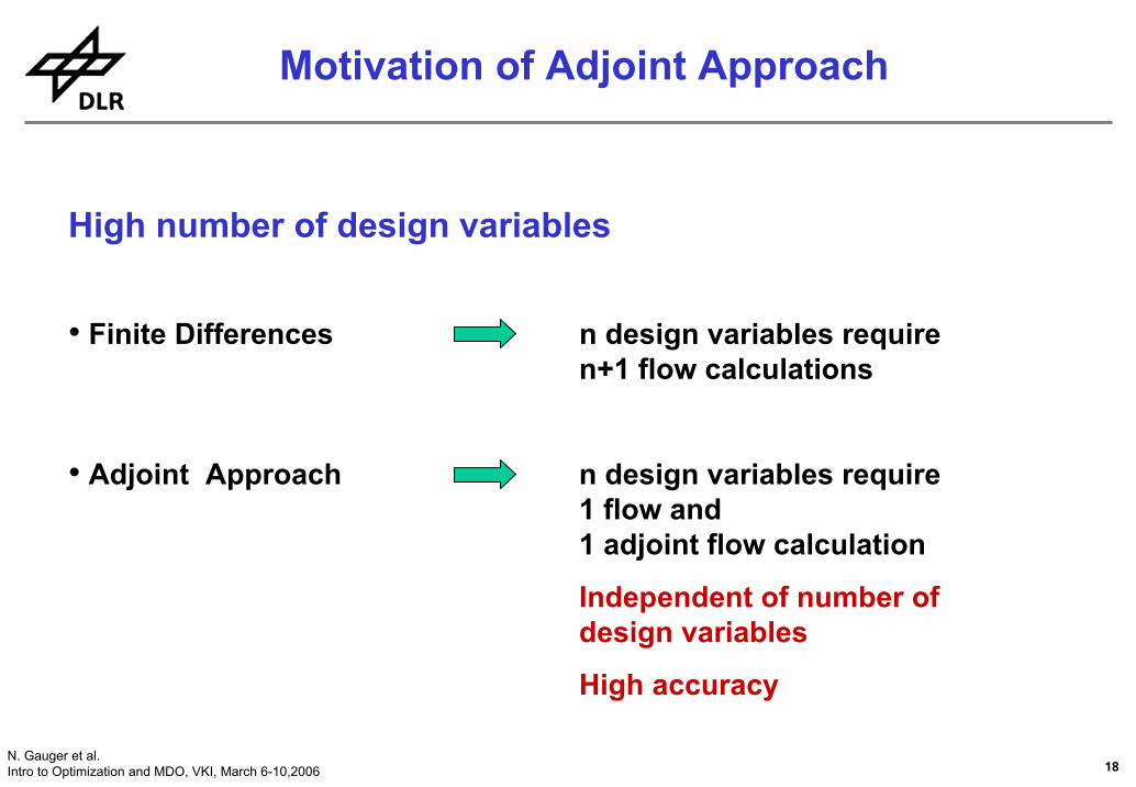
High number of design variables
• Finite Differences n design variables require n+1 flow calculations
• Adjoint Approach n design variables require 1 flow and1 adjoint flow calculation
Independent of number of design variables
High accuracy
Motivation of Adjoint Approach
19N. Gauger et al.Intro to Optimization and MDO, VKI, March 6-10,2006
20N. Gauger et al.Intro to Optimization and MDO, VKI, March 6-10,2006
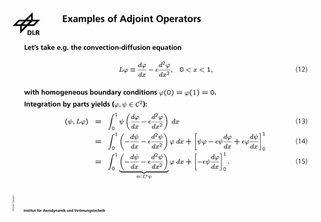
21N. Gauger et al.Intro to Optimization and MDO, VKI, March 6-10,2006
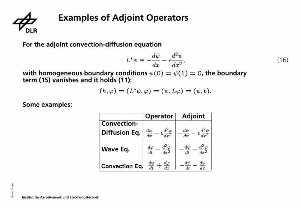
22N. Gauger et al.Intro to Optimization and MDO, VKI, March 6-10,2006
Convection Eq.
23N. Gauger et al.Intro to Optimization and MDO, VKI, March 6-10,2006
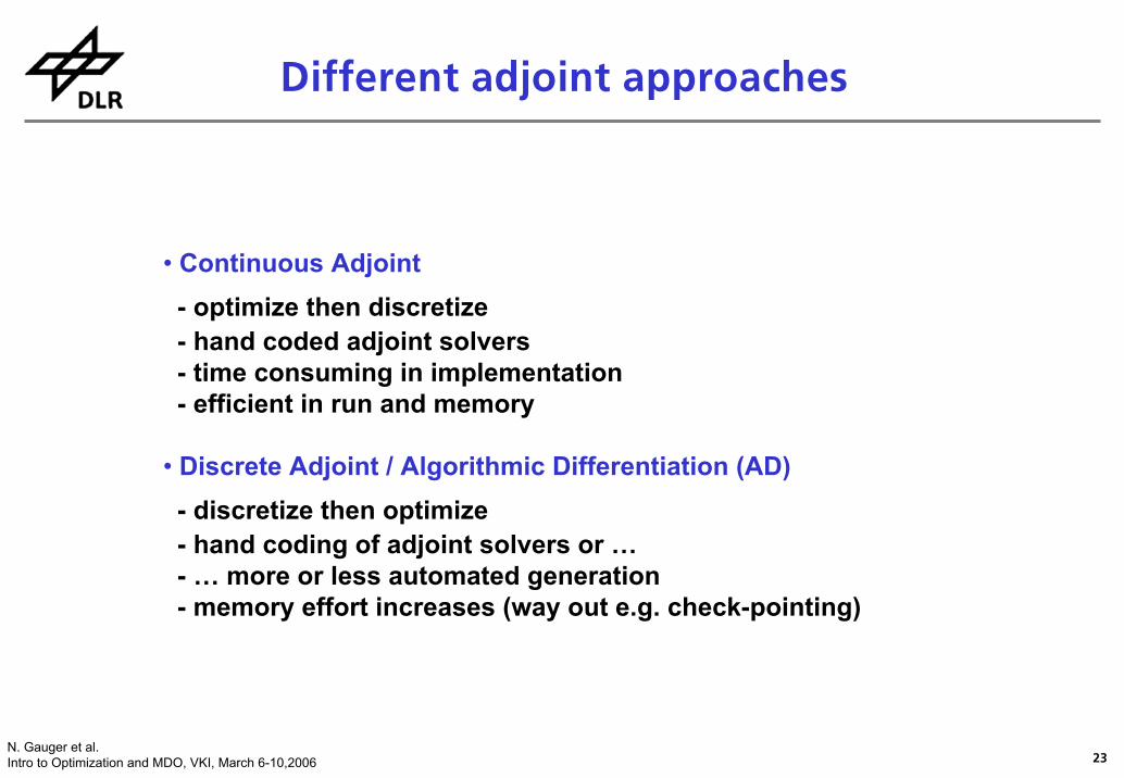
• Continuous Adjoint- optimize then discretize- hand coded adjoint solvers- time consuming in implementation- efficient in run and memory
• Discrete Adjoint / Algorithmic Differentiation (AD)- discretize then optimize- hand coding of adjoint solvers or …- … more or less automated generation- memory effort increases (way out e.g. check-pointing)
Different adjoint approaches
24N. Gauger et al.Intro to Optimization and MDO, VKI, March 6-10,2006
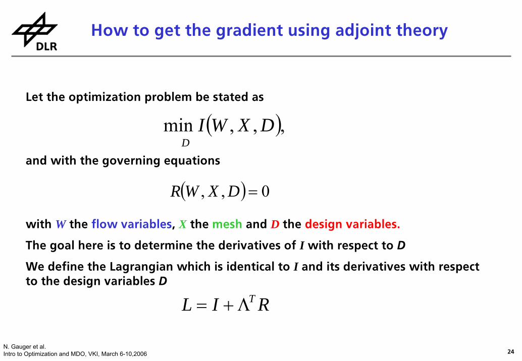
How to get the gradient using adjoint theory
Let the optimization problem be stated as
and with the governing equations
with W the flow variables, X the mesh and D the design variables.
The goal here is to determine the derivatives of I with respect to D
We define the Lagrangian which is identical to I and its derivatives with respect to the design variables D
( ) 0,, =DXWR
( ),,, min D
DXWI
RIL TΛ+=
25N. Gauger et al.Intro to Optimization and MDO, VKI, March 6-10,2006
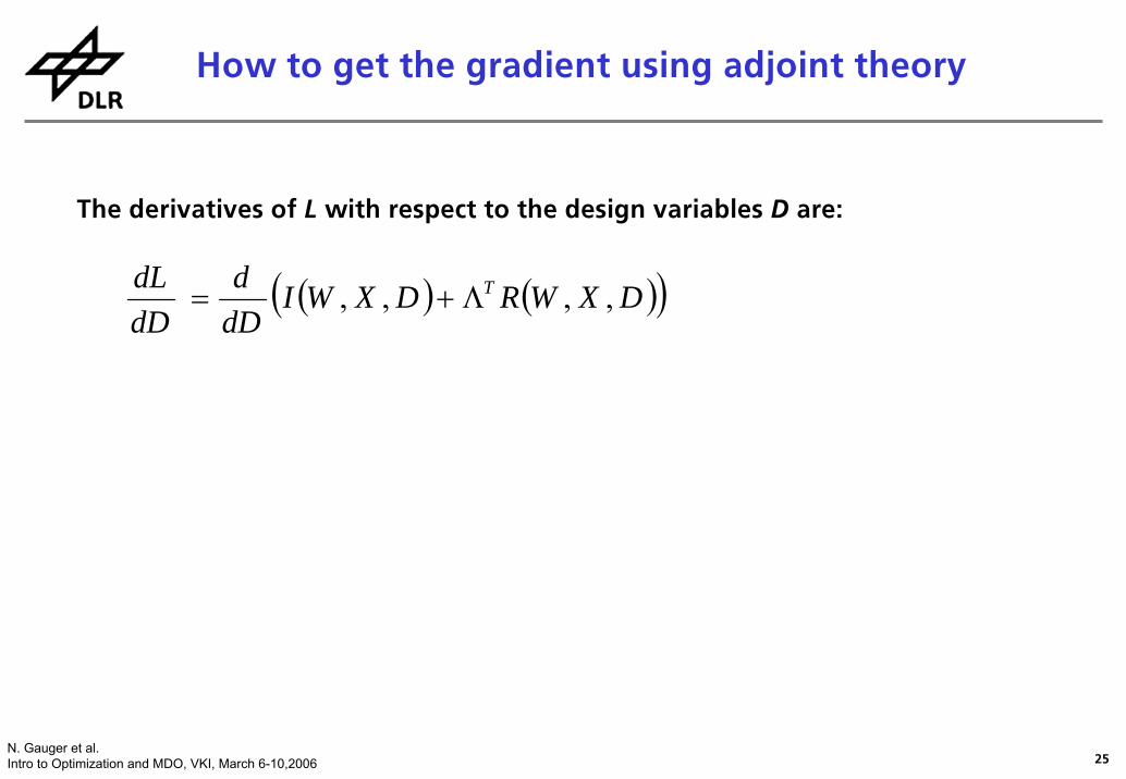
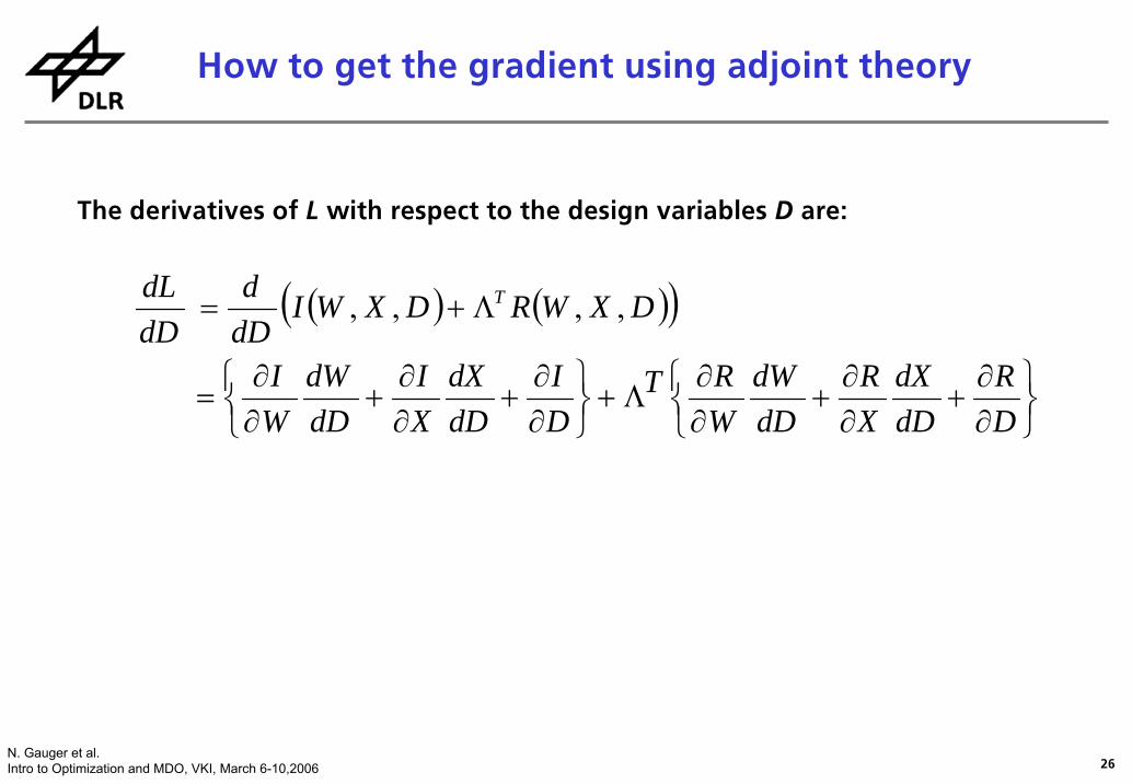
The derivatives of L with respect to the design variables D are:
( ) ( )( )Λ+= DXWRDXWIdDd
dDdL T ,,,,
How to get the gradient using adjoint theory
26N. Gauger et al.Intro to Optimization and MDO, VKI, March 6-10,2006
( ) ( )( )
⎭⎬⎫
⎩⎨⎧
∂∂
+∂∂
+∂∂
Λ+⎭⎬⎫
⎩⎨⎧
∂∂
+∂∂
+∂∂
=
Λ+=
DR
dDdX
XR
dDdW
WRT
DI
dDdX
XI
dDdW
WI
DXWRDXWIdDd
dDdL T
,,,,
The derivatives of L with respect to the design variables D are:
How to get the gradient using adjoint theory
27N. Gauger et al.Intro to Optimization and MDO, VKI, March 6-10,2006
( ) ( )( )
⎭⎬⎫
⎩⎨⎧
∂∂
Λ+∂∂
+⎭⎬⎫
⎩⎨⎧
∂∂
Λ+∂∂
+⎭⎬⎫
⎩⎨⎧
∂∂
Λ+∂∂
=
⎭⎬⎫
⎩⎨⎧
∂∂
+∂∂
+∂∂
Λ+⎭⎬⎫
⎩⎨⎧
∂∂
+∂∂
+∂∂
=
Λ+=
DRT
DI
dDdX
XRT
XI
dDdW
WRT
WI
DR
dDdX
XR
dDdW
WRT
DI
dDdX
XI
dDdW
WI
DXWRDXWIdDd
dDdL T
,,,,
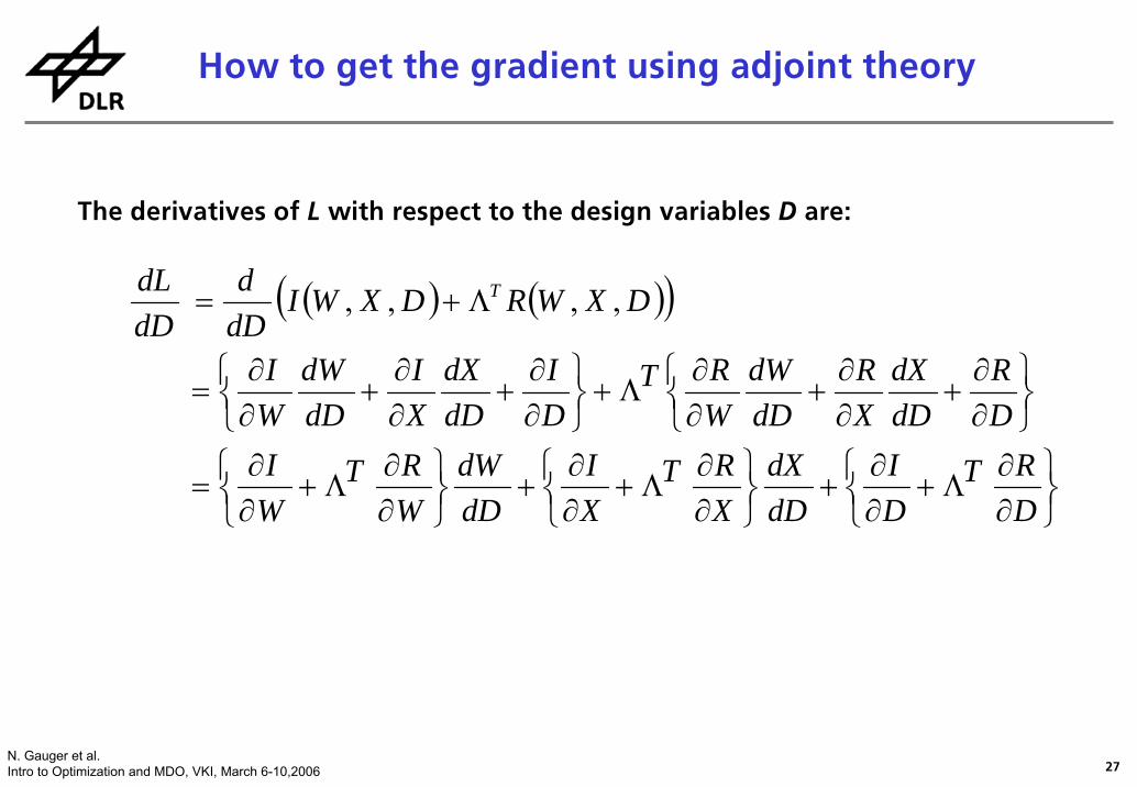
The derivatives of L with respect to the design variables D are:
How to get the gradient using adjoint theory
28N. Gauger et al.Intro to Optimization and MDO, VKI, March 6-10,2006
=0
}
}}
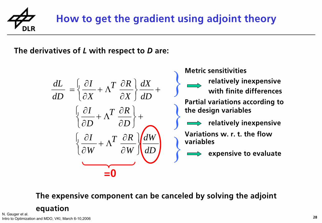
The expensive component can be canceled by solving the adjoint
The derivatives of L with respect to D are:
equation
dDdW
WRT
WI
DRT
DI
dDdX
XRT
XI
dDdL
⎭⎬⎫
⎩⎨⎧
∂∂
Λ+∂∂
+⎭⎬⎫
⎩⎨⎧
∂∂
Λ+∂∂
+⎭⎬⎫
⎩⎨⎧
∂∂
Λ+∂∂
=
Variations w. r. t. the flow variables
expensive to evaluate
Partial variations according to the design variables
relatively inexpensive
Metric sensitivities
relatively inexpensive with finite differences
How to get the gradient using adjoint theory
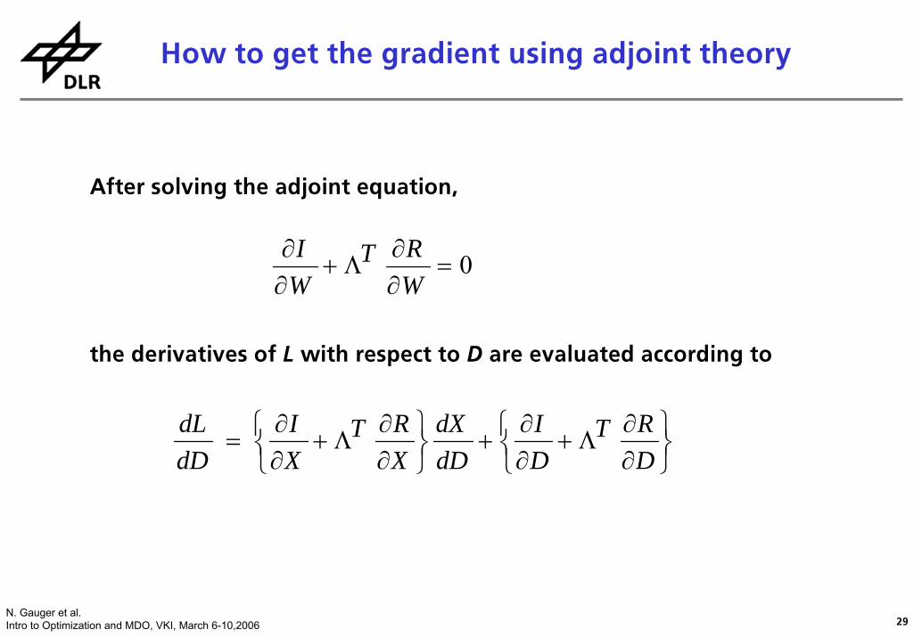
29N. Gauger et al.Intro to Optimization and MDO, VKI, March 6-10,2006
After solving the adjoint equation,
the derivatives of L with respect to D are evaluated according to
⎭⎬⎫
⎩⎨⎧
∂∂
Λ+∂∂
+⎭⎬⎫
⎩⎨⎧
∂∂
Λ+∂∂
=DRT
DI
dDdX
XRT
XI
dDdL
0=∂∂
Λ+∂∂
WRT
WI
How to get the gradient using adjoint theory
30N. Gauger et al.Intro to Optimization and MDO, VKI, March 6-10,2006
31N. Gauger et al.Intro to Optimization and MDO, VKI, March 6-10,2006
32N. Gauger et al.Intro to Optimization and MDO, VKI, March 6-10,2006
33N. Gauger et al.Intro to Optimization and MDO, VKI, March 6-10,2006
34N. Gauger et al.Intro to Optimization and MDO, VKI, March 6-10,2006
35N. Gauger et al.Intro to Optimization and MDO, VKI, March 6-10,2006
36N. Gauger et al.Intro to Optimization and MDO, VKI, March 6-10,2006
37N. Gauger et al.Intro to Optimization and MDO, VKI, March 6-10,2006
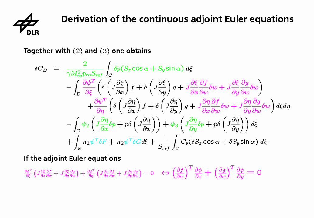
0=∂∂
⎟⎠⎞
⎜⎝⎛
∂∂
−∂∂
⎟⎠⎞
⎜⎝⎛
∂∂
−∂
∂−
ywg
xwf
t
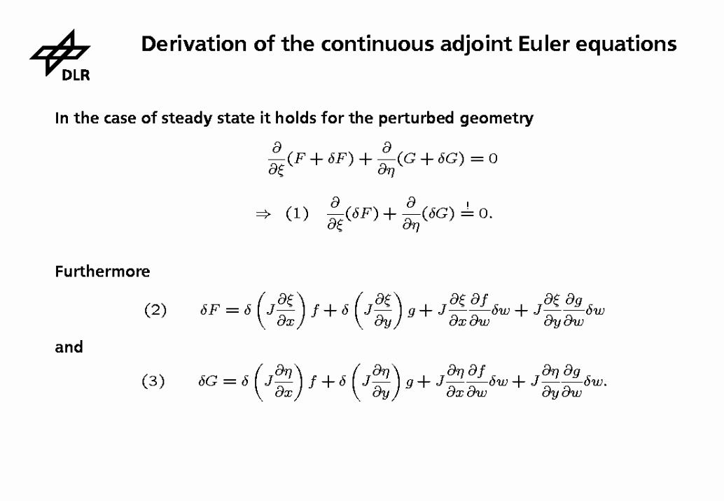
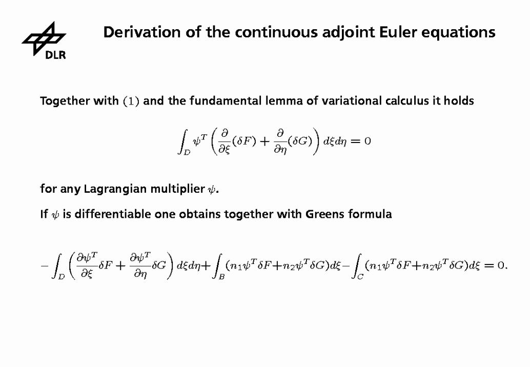
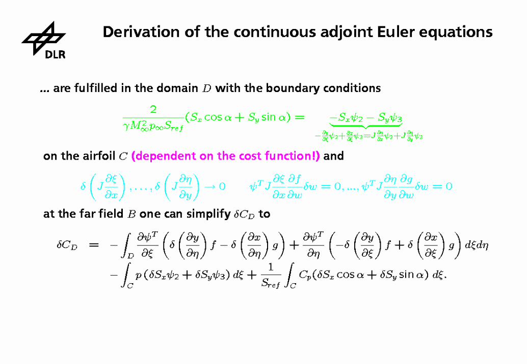
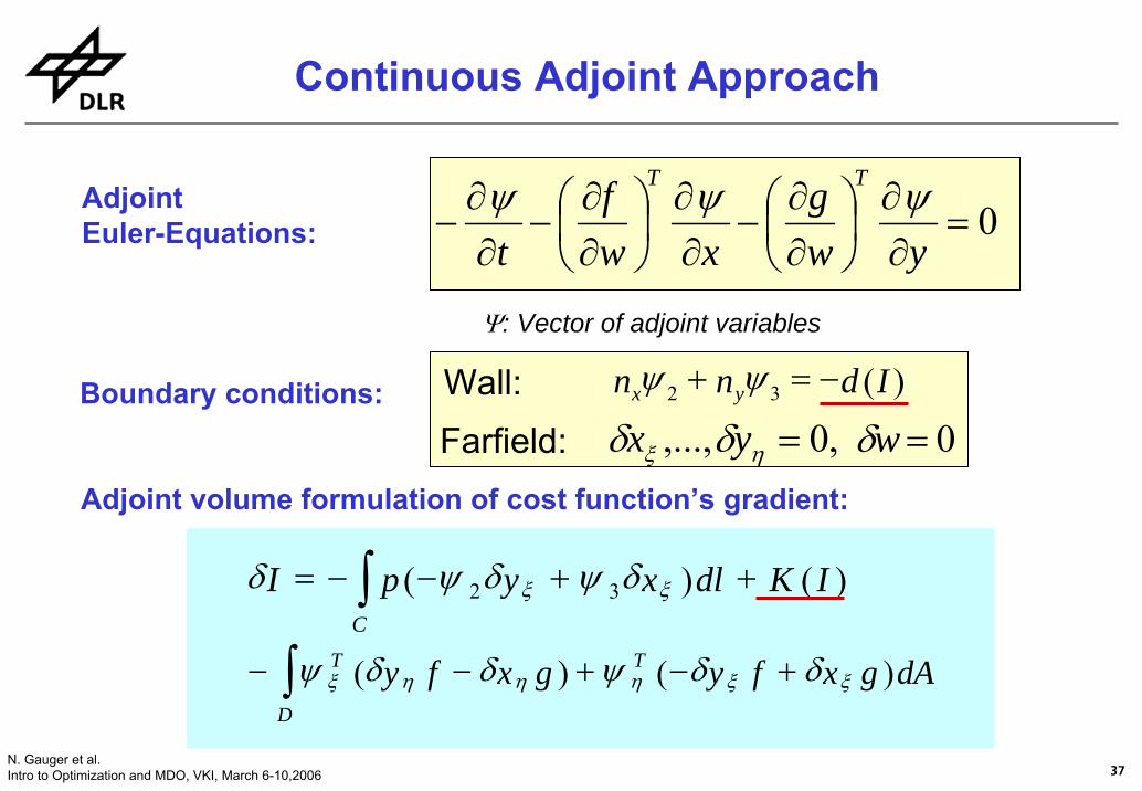
TT ψψψAdjointEuler-Equations:
Boundary conditions:
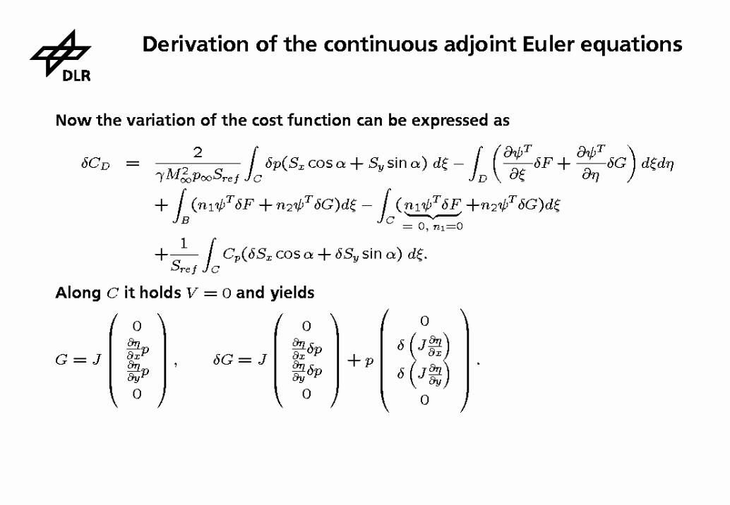
∫ ++−−=C
IKdlxypI )()( 32 ξξ δψδψδ
∫ +−+−−D
TT dAgxfygxfy )()( ξξηηηξ δδψδδψ
Adjoint volume formulation of cost function’s gradient:
Ψ: Vector of adjoint variables
)(32 Idnn yx −=+ ψψ
0=wδ,0,..., =ηξ δδ yxWall:Farfield:
Continuous Adjoint Approach
38N. Gauger et al.Intro to Optimization and MDO, VKI, March 6-10,2006
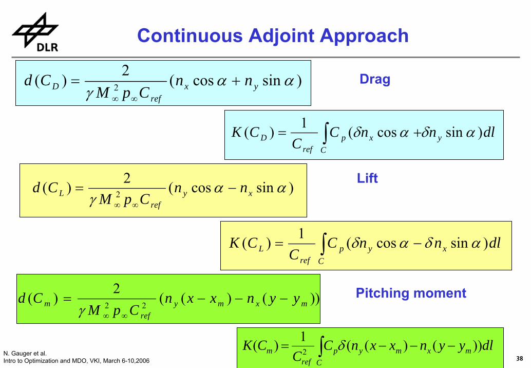
)sincos(2)( 2 ααγ yx
refD nn
CpMCd +=
∞∞
dlnnCC
CK yC
xpref
D )sincos(1)( αδαδ∫ +=
)sincos(2)( 2 ααγ xy
refL nn
CpMCd −=
∞∞
dlnnCC
CK xC
ypref
L )sincos(1)( αδαδ∫ −=
))()((2
)(22 mxmyref
m yynxxnCpM
Cd −−−=∞∞γ
dlyynxxnCC
CKC
mxmypref
m ))()((1)( 2 ∫ −−−= δ
Drag
Pitching moment
Lift
Continuous Adjoint Approach
39N. Gauger et al.Intro to Optimization and MDO, VKI, March 6-10,2006
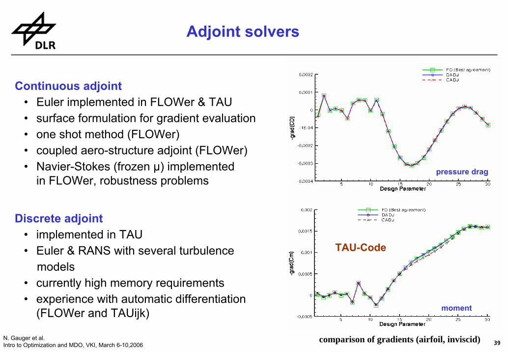
Continuous adjoint• Euler implemented in FLOWer & TAU• surface formulation for gradient evaluation• one shot method (FLOWer)• coupled aero-structure adjoint (FLOWer) • Navier-Stokes (frozen μ) implemented
in FLOWer, robustness problems
Discrete adjoint• implemented in TAU • Euler & RANS with several turbulence
models• currently high memory requirements• experience with automatic differentiation
(FLOWer and TAUijk) moment
pressure drag
TAU-Code
comparison of gradients (airfoil, inviscid)
Adjoint solvers
40N. Gauger et al.Intro to Optimization and MDO, VKI, March 6-10,2006
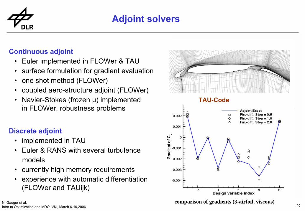
Continuous adjoint• Euler implemented in FLOWer & TAU• surface formulation for gradient evaluation• one shot method (FLOWer)• coupled aero-structure adjoint (FLOWer) • Navier-Stokes (frozen μ) implemented
in FLOWer, robustness problems
Discrete adjoint• implemented in TAU • Euler & RANS with several turbulence
models• currently high memory requirements• experience with automatic differentiation
(FLOWer and TAUijk) moment
pressure drag
comparison of gradients (airfoil, inviscid)
TAU-Code
comparison of gradients (3-airfoil, viscous)
TAU-Code
Adjoint solvers
41N. Gauger et al.Intro to Optimization and MDO, VKI, March 6-10,2006
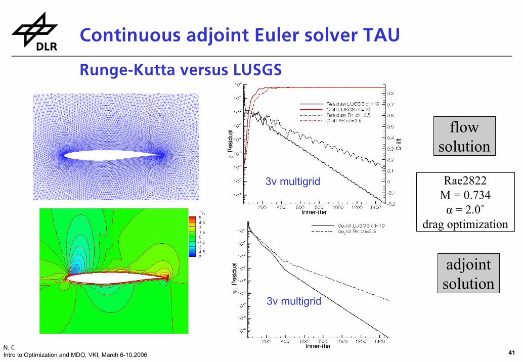
flowsolution
Rae2822M = 0.734α = 2.0˚
drag optimization
adjointsolution
3v multigrid
3v multigrid
Continuous adjoint Euler solver TAU
Runge-Kutta versus LUSGS
42N. Gauger et al.Intro to Optimization and MDO, VKI, March 6-10,2006
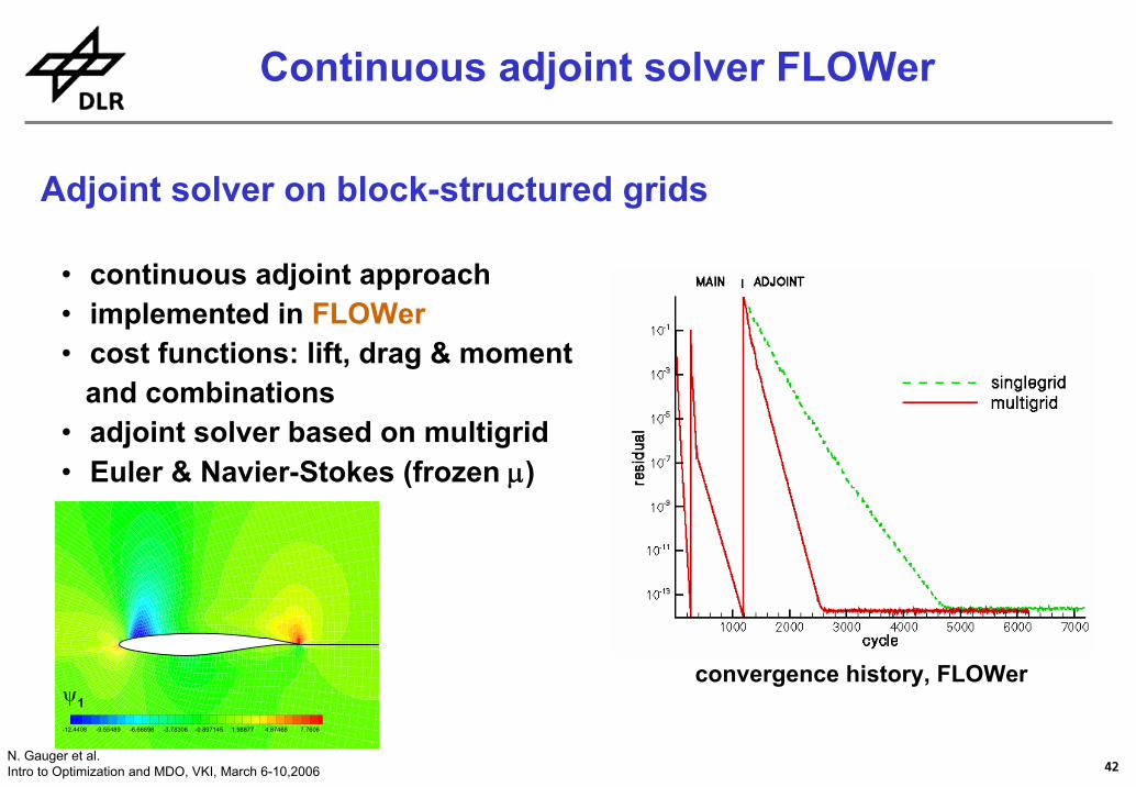
Continuous adjoint solver FLOWer
Adjoint solver on block-structured grids
• continuous adjoint approach• implemented in FLOWer• cost functions: lift, drag & moment
and combinations • adjoint solver based on multigrid• Euler & Navier-Stokes (frozen μ)
convergence history, FLOWer
-12.4408 -9.55489 -6.66898 -3.78306 -0.897145 1.98877 4.87468 7.7606
ψ1
43N. Gauger et al.Intro to Optimization and MDO, VKI, March 6-10,2006
n-th Design Variable
-∇C
m
0 10 20 30 40 50-5
-4
-3
-2
-1
0
1
2
AdjointFinite Differences
n-th Design Variable
-∇C
L
0 10 20 30 40 50-18
-16
-14
-12
-10
-8
-6
-4
-2
0
2
AdjointFinite Differences
n-th Design Variable
-∇C
D
0 10 20 30 40 50-0.8
-0.6
-0.4
-0.2
0
0.2
0.4
0.6
0.8
AdjointFinite Differences
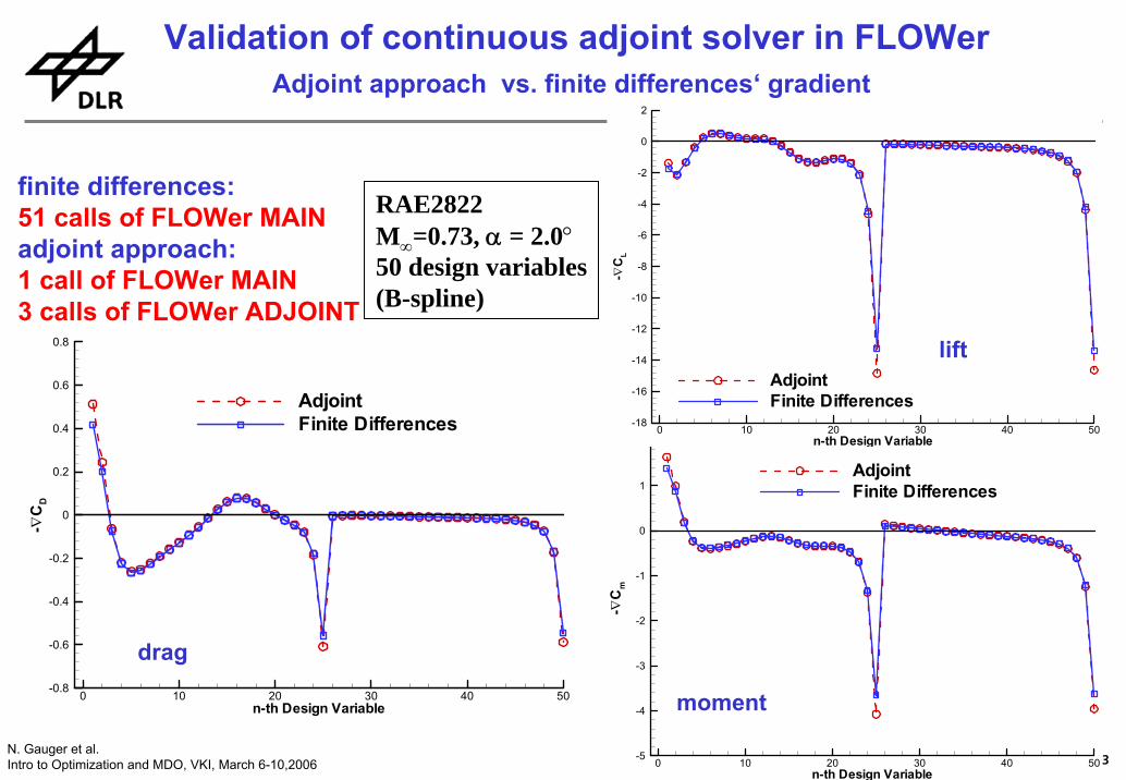
RAE2822M∞=0.73, α = 2.0°50 design variables(B-spline)
Validation of continuous adjoint solver in FLOWerAdjoint approach vs. finite differences‘ gradient
drag
lift
moment
finite differences: 51 calls of FLOWer MAINadjoint approach:1 call of FLOWer MAIN3 calls of FLOWer ADJOINT
44N. Gauger et al.Intro to Optimization and MDO, VKI, March 6-10,2006
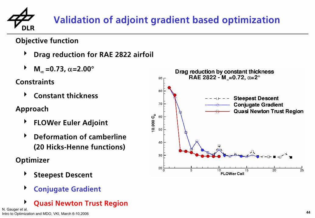
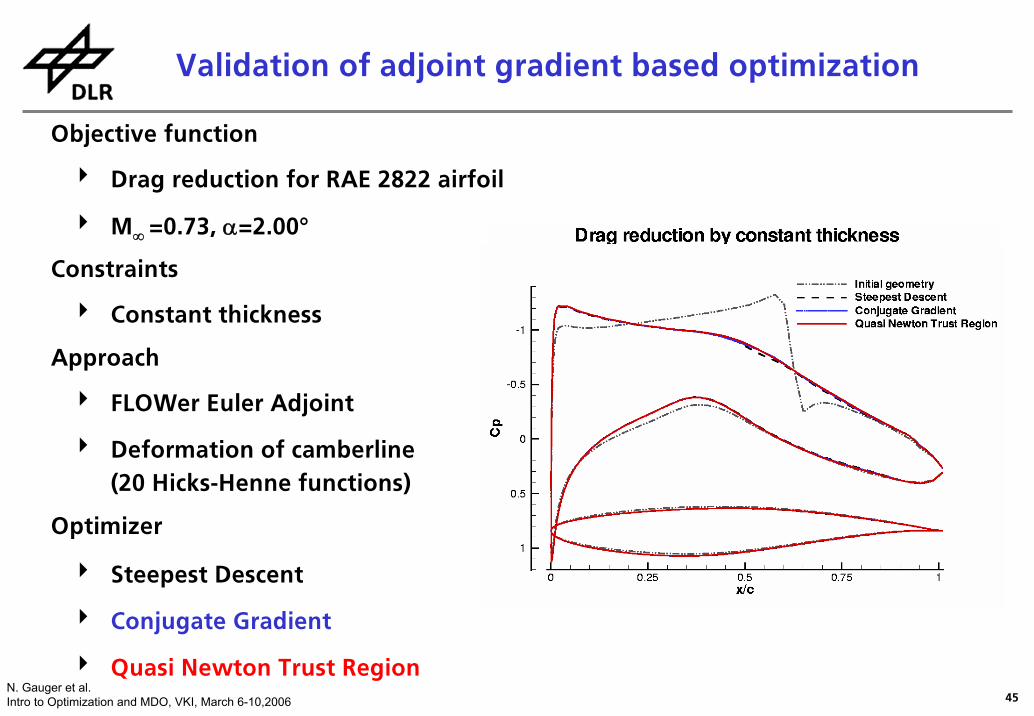
Validation of adjoint gradient based optimization
Objective function
4 Drag reduction for RAE 2822 airfoil
4 M∞ =0.73, α=2.00°
Constraints
4 Constant thickness
Approach
4 FLOWer Euler Adjoint
4 Deformation of camberline(20 Hicks-Henne functions)
Optimizer
4 Steepest Descent
4 Conjugate Gradient
4 Quasi Newton Trust Region
45N. Gauger et al.Intro to Optimization and MDO, VKI, March 6-10,2006
Validation of adjoint gradient based optimization
Objective function
4 Drag reduction for RAE 2822 airfoil
4 M∞ =0.73, α=2.00°
Constraints
4 Constant thickness
Approach
4 FLOWer Euler Adjoint
4 Deformation of camberline(20 Hicks-Henne functions)
Optimizer
4 Steepest Descent
4 Conjugate Gradient
4 Quasi Newton Trust Region
46N. Gauger et al.Intro to Optimization and MDO, VKI, March 6-10,2006
Content of lecture
Why adjoint approaches?
What is an adjoint approach?
Continuous and discrete adjoint approaches / solvers
Validation and Application in 2D and 3D, Euler and Navier-Stokes
Algorithmic / Automated Differentiation (AD)
Coupled aero-structure adjoint approach
Validation and application in MDO context
One shot approaches
Adjoint Approaches in Aerodynamic Shape Optimization and MDO Context II
47N. Gauger et al.Intro to Optimization and MDO, VKI, March 6-10,2006
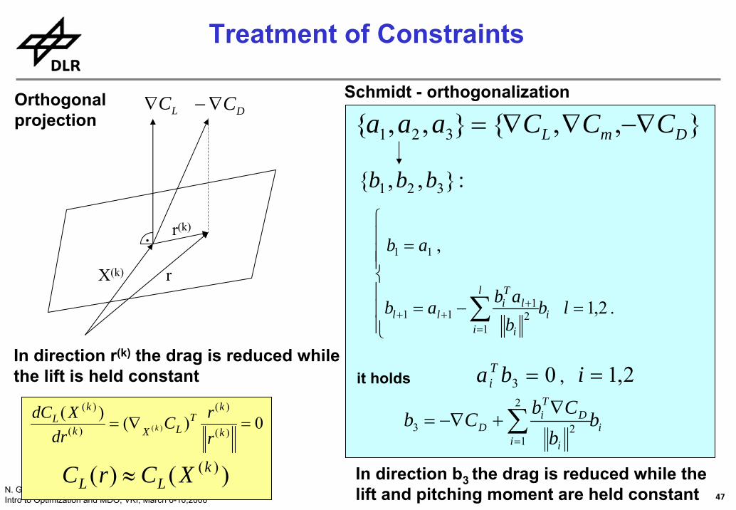
Orthogonalprojection
ii i
DTi
D bb
CbCb ∑=
∇+−∇=
2
123
03 =ba Ti , 2,1=i
⎪⎪⎪
⎩
⎪⎪⎪
⎨
⎧
=−=
=
∑=
+++ . 2,1
,
12
111
11
lbbabab
ab
i
l
i i
lTi
ll
},,{},,{ 321 DmL CCCaaa −∇∇∇=
)()( )(kLL XCrC ≈
0)()()(
)(
)(
)(
)( =∇=k
kT
LXk
kL
rrC
drXdC
k
},,{ 321 bbb
Schmidt - orthogonalization
:
In direction b3 the drag is reduced while thelift and pitching moment are held constant
it holdsIn direction r(k) the drag is reduced whilethe lift is held constant
.
X(k)
LC∇ DC∇−
r(k)
r
Treatment of Constraints
48N. Gauger et al.Intro to Optimization and MDO, VKI, March 6-10,2006
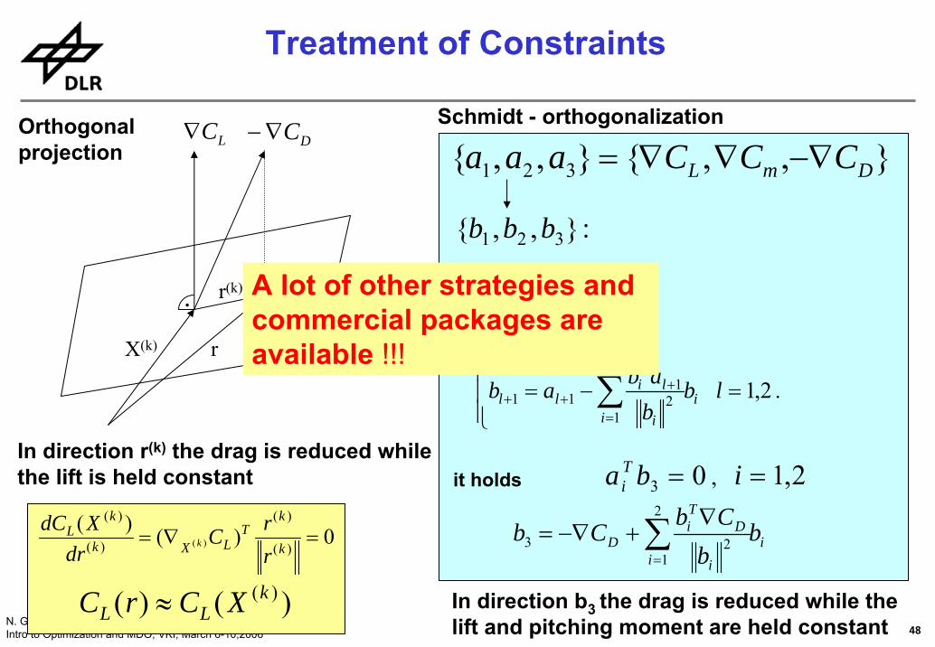
Orthogonalprojection
ii i
DTi
D bb
CbCb ∑=
∇+−∇=
2
123
03 =ba Ti , 2,1=i
⎪⎪⎪
⎩
⎪⎪⎪
⎨
⎧
=−=
=
∑=
+++ . 2,1
,
12
111
11
lbbabab
ab
i
l
i i
lTi
ll
},,{},,{ 321 DmL CCCaaa −∇∇∇=
)()( )(kLL XCrC ≈
0)()()(
)(
)(
)(
)( =∇=k
kT
LXk
kL
rrC
drXdC
k
},,{ 321 bbb
Schmidt - orthogonalization
:
In direction b3 the drag is reduced while thelift and pitching moment are held constant
it holdsIn direction r(k) the drag is reduced whilethe lift is held constant
.
X(k)
LC∇ DC∇−
r(k)
r
Treatment of Constraints
A lot of other strategies andcommercial packages areavailable !!!
49N. Gauger et al.Intro to Optimization and MDO, VKI, March 6-10,2006
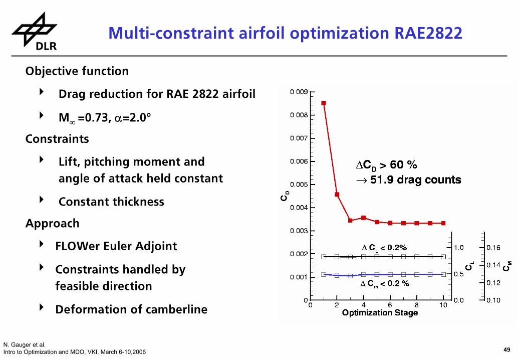
Objective function
4 Drag reduction for RAE 2822 airfoil
4 M∞ =0.73, α=2.0°
Constraints
4 Lift, pitching moment and angle of attack held constant
4 Constant thickness
Approach
4 FLOWer Euler Adjoint
4 Constraints handled byfeasible direction
4 Deformation of camberline
Multi-constraint airfoil optimization RAE2822
50N. Gauger et al.Intro to Optimization and MDO, VKI, March 6-10,2006
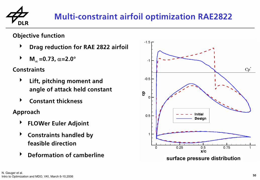
Objective function
4 Drag reduction for RAE 2822 airfoil
4 M∞ =0.73, α=2.0°
Constraints
4 Lift, pitching moment and angle of attack held constant
4 Constant thickness
Approach
4 FLOWer Euler Adjoint
4 Constraints handled byfeasible direction
4 Deformation of camberline
Multi-constraint airfoil optimization RAE2822
surface pressure distribution
51N. Gauger et al.Intro to Optimization and MDO, VKI, March 6-10,2006
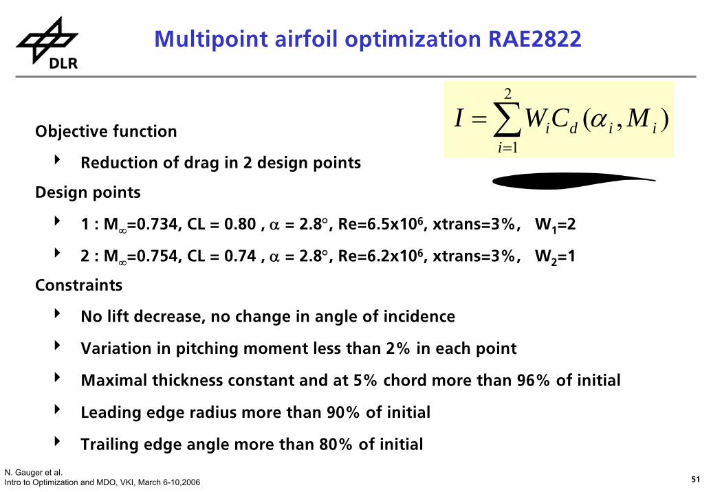
Objective function
4 Reduction of drag in 2 design points
Design points
4 1 : M∞=0.734, CL = 0.80 , α = 2.8°, Re=6.5x10⁶, xtrans=3%, W1=2
4 2 : M∞=0.754, CL = 0.74 , α = 2.8°, Re=6.2x10⁶, xtrans=3%, W2=1
Constraints
4 No lift decrease, no change in angle of incidence
4 Variation in pitching moment less than 2% in each point
4 Maximal thickness constant and at 5% chord more than 96% of initial
4 Leading edge radius more than 90% of initial
4 Trailing edge angle more than 80% of initial
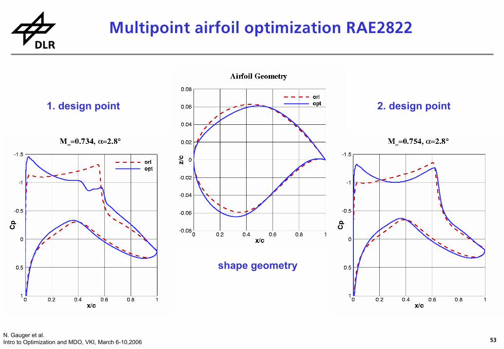
Multipoint airfoil optimization RAE2822
),(2
1iid
ii MCWI α∑
=
=
52N. Gauger et al.Intro to Optimization and MDO, VKI, March 6-10,2006
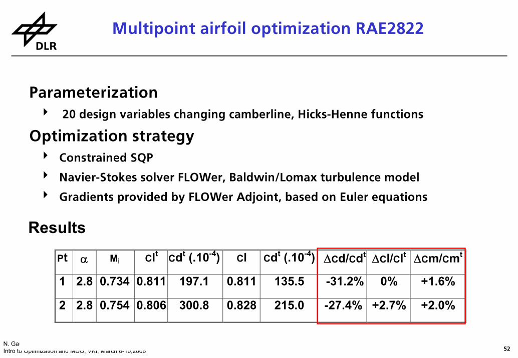
Parameterization4 20 design variables changing camberline, Hicks-Henne functions
Optimization strategy4 Constrained SQP
4 Navier-Stokes solver FLOWer, Baldwin/Lomax turbulence model
4 Gradients provided by FLOWer Adjoint, based on Euler equations
Results
Pt α Mi Clt Cdt (.10-4) Cl Cdt (.10-4) ΔCd/Cdt ΔCl/Clt ΔCm/Cmt
1 2.8 0.734 0.811 197.1 0.811 135.5 -31.2% 0% +1.6%
2 2.8 0.754 0.806 300.8 0.828 215.0 -27.4% +2.7% +2.0%
Multipoint airfoil optimization RAE2822
53N. Gauger et al.Intro to Optimization and MDO, VKI, March 6-10,2006
1. design point 2. design point
shape geometry
Multipoint airfoil optimization RAE2822
54N. Gauger et al.Intro to Optimization and MDO, VKI, March 6-10,2006
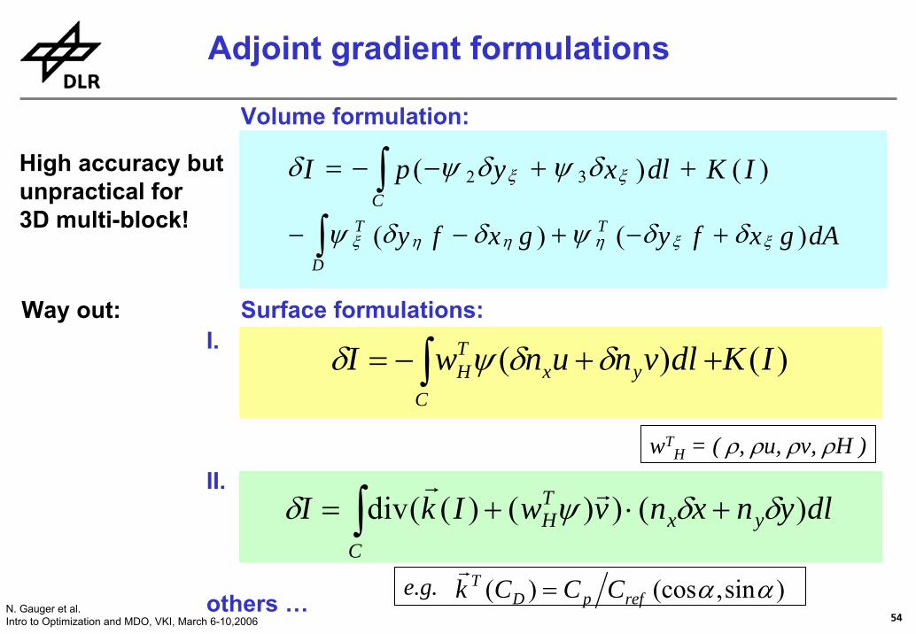
Volume formulation:
Surface formulations:
Adjoint gradient formulations
∫ ++−−=C
IKdlxypI )()( 32 ξξ δψδψδ
∫ +−+−−D
TT dAgxfygxfy )()( ξξηηηξ δδψδδψ
)()( IKdlvnunwIC
yxTH∫ ++−= δδψδ
wTH = ( ρ, ρu, ρv, ρH )
∫ +⋅+=C
yxTH dlynxnvwIkI )())()((div δδψδ rr
e.g. )sin,(cos)( ααrefpDT CCCk =r
High accuracy butunpractical for 3D multi-block!
Way out:
II.
I.
others …
55N. Gauger et al.Intro to Optimization and MDO, VKI, March 6-10,2006
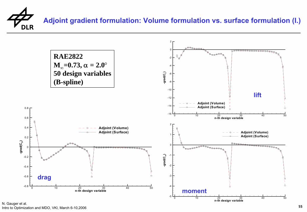
n-th design variable
-gra
d(C
L)
0 10 20 30 40 50-16
-14
-12
-10
-8
-6
-4
-2
0
2
Adjoint (Volume)Adjoint (Surface)
n-th design variable
-gra
d(C
m)
0 10 20 30 40 50-5
-4
-3
-2
-1
0
1
2
Adjoint (Volume)Adjoint (Surface)
n-th design variable
-gra
d(C
D)
0 10 20 30 40 50-0.8
-0.6
-0.4
-0.2
0
0.2
0.4
0.6
0.8
Adjoint (Volume)Adjoint (Surface)
RAE2822M∞=0.73, α = 2.0°50 design variables(B-spline)
Adjoint gradient formulation: Volume formulation vs. surface formulation (I.)
drag
lift
moment
56N. Gauger et al.Intro to Optimization and MDO, VKI, March 6-10,2006
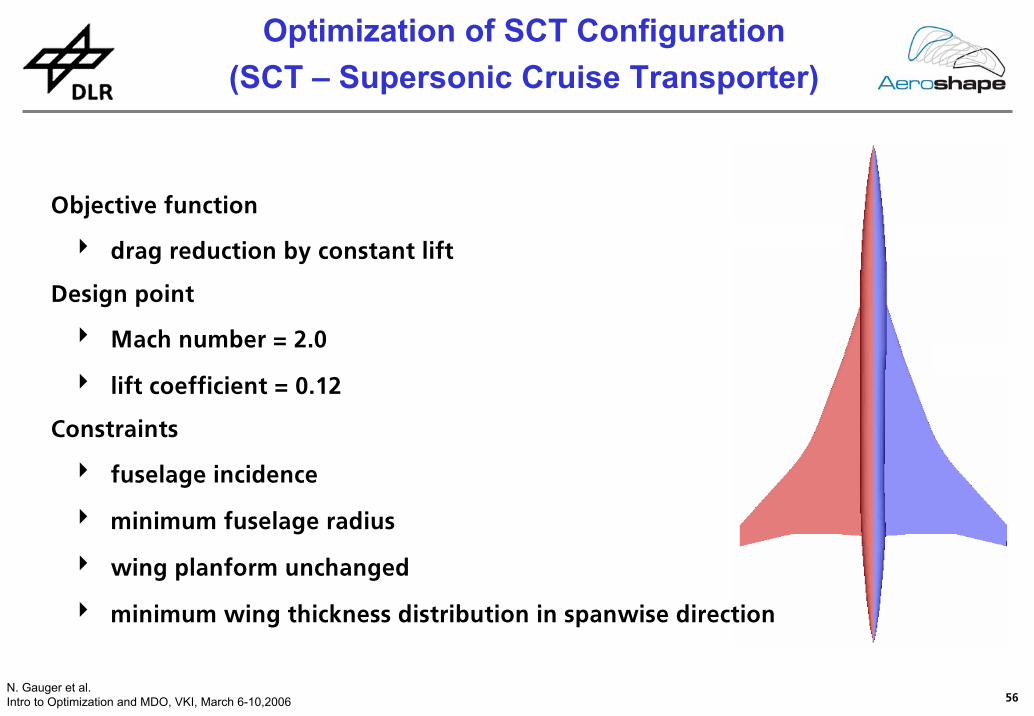
Objective function
4 drag reduction by constant lift
Design point
4 Mach number = 2.0
4 lift coefficient = 0.12
Constraints
4 fuselage incidence
4 minimum fuselage radius
4 wing planform unchanged
4 minimum wing thickness distribution in spanwise direction
Optimization of SCT Configuration (SCT – Supersonic Cruise Transporter)
57N. Gauger et al.Intro to Optimization and MDO, VKI, March 6-10,2006
Approach
4 FLOWer code in Euler mode with target lift option
4 Lift kept constant by adjusting angle of attack
4 FLOWer code in Euler adjoint mode
4 Adjoint gradient formulation: Surface formulation (II.)
4 Structured mono-block grid (MegaCads), 230.000 grid points
Optimization strategy
4 Quasi-Newton Method (BFGS algorithm)
Optimization of SCT Configuration
58N. Gauger et al.Intro to Optimization and MDO, VKI, March 6-10,2006
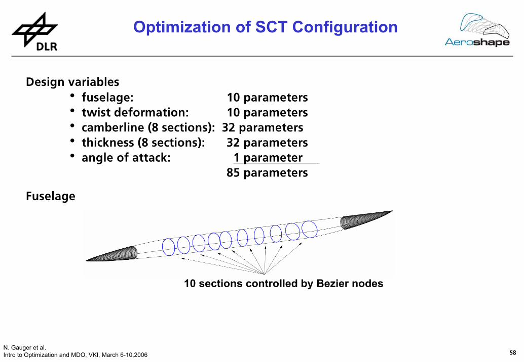
Fuselage
10 sections controlled by Bezier nodes
Design variables h fuselage: 10 parametersh twist deformation: 10 parametersh camberline (8 sections): 32 parametersh thickness (8 sections): 32 parametersh angle of attack: 1 parameter .
85 parameters
Optimization of SCT Configuration
59N. Gauger et al.Intro to Optimization and MDO, VKI, March 6-10,2006
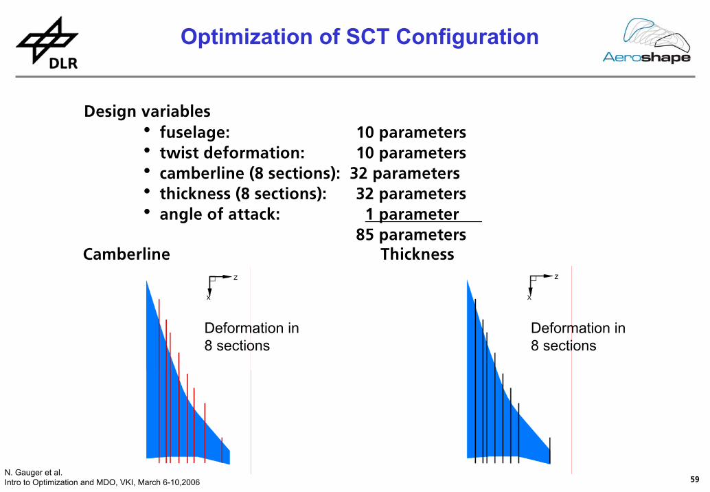
Camberline Thickness
Deformation in8 sections
Deformation in 8 sections
Design variables h fuselage: 10 parametersh twist deformation: 10 parametersh camberline (8 sections): 32 parametersh thickness (8 sections): 32 parametersh angle of attack: 1 parameter .
85 parameters
Optimization of SCT Configuration
60N. Gauger et al.Intro to Optimization and MDO, VKI, March 6-10,2006
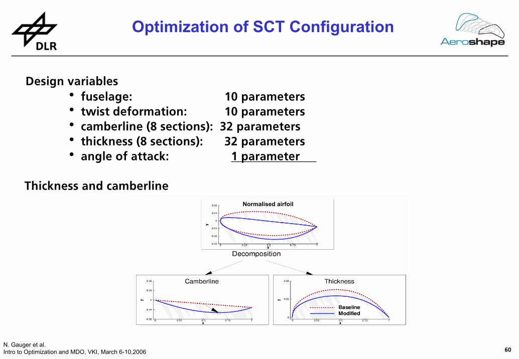
Design variables h fuselage: 10 parametersh twist deformation: 10 parametersh camberline (8 sections): 32 parametersh thickness (8 sections): 32 parametersh angle of attack: 1 parameter .
85 parametersThickness and camberline
Normalised airfoil
Optimization of SCT Configuration
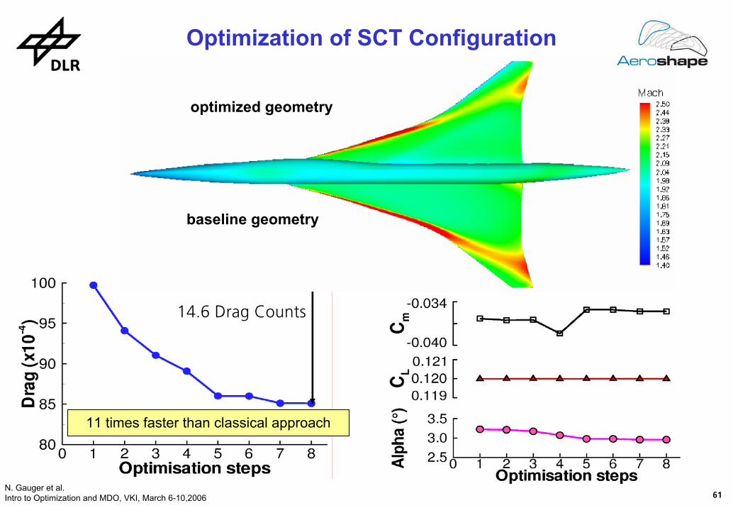
61N. Gauger et al.Intro to Optimization and MDO, VKI, March 6-10,2006
11 times faster than classical approach
14.6 Drag Counts
optimized geometry
baseline geometry
Optimization of SCT Configuration
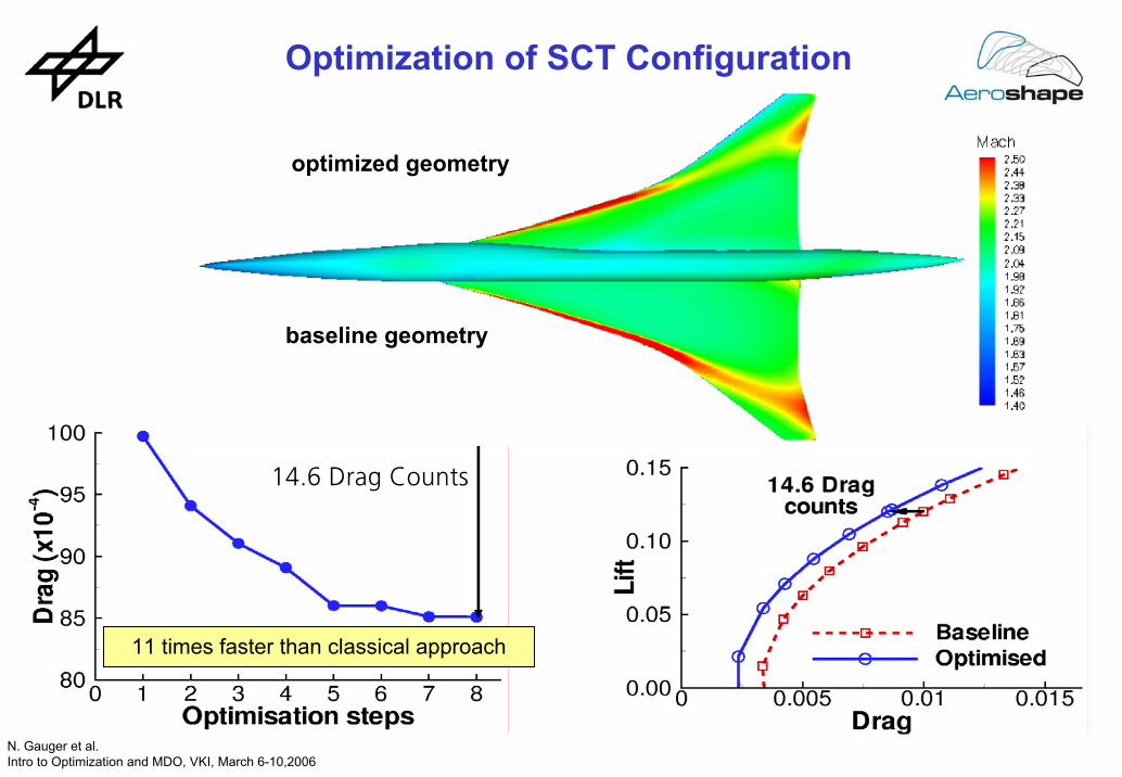
62N. Gauger et al.Intro to Optimization and MDO, VKI, March 6-10,2006
11 times faster than classical approach
14.6 Drag Counts
optimized geometry
baseline geometry
Optimization of SCT Configuration
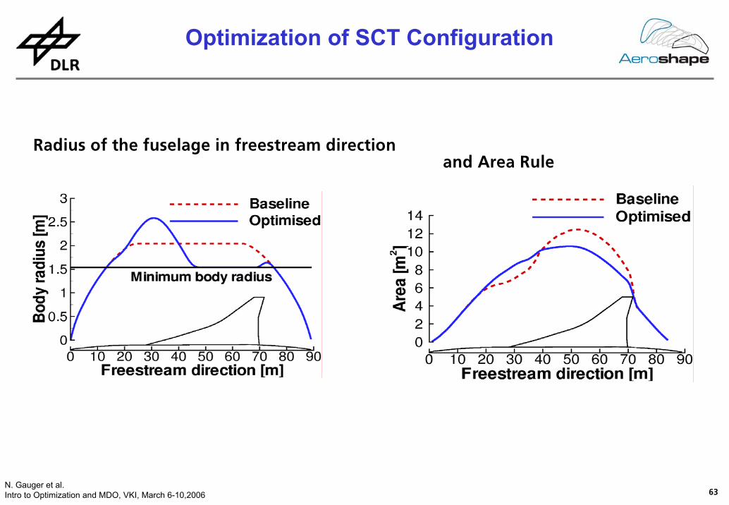
63N. Gauger et al.Intro to Optimization and MDO, VKI, March 6-10,2006
and Area RuleRadius of the fuselage in freestream direction
Optimization of SCT Configuration
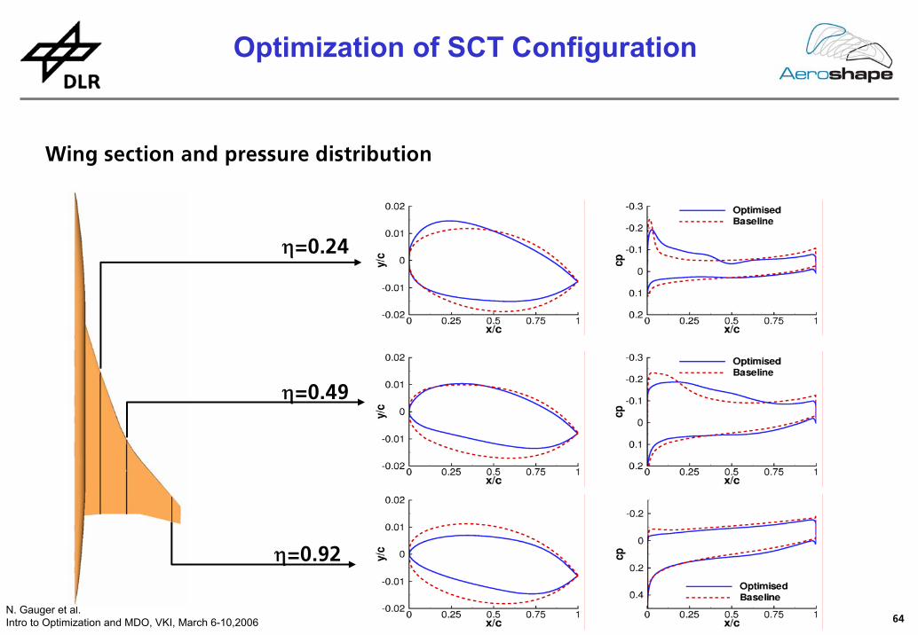
64N. Gauger et al.Intro to Optimization and MDO, VKI, March 6-10,2006
Wing section and pressure distribution
η=0.24
η=0.49
η=0.92
Optimization of SCT Configuration
65N. Gauger et al.Intro to Optimization and MDO, VKI, March 6-10,2006
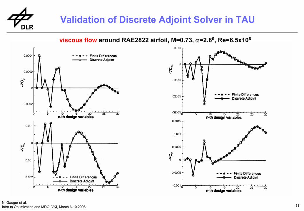
Validation of Discrete Adjoint Solver in TAU
viscous flow around RAE2822 airfoil, M=0.73, α=2.80, Re=6.5x10⁶
66N. Gauger et al.Intro to Optimization and MDO, VKI, March 6-10,2006
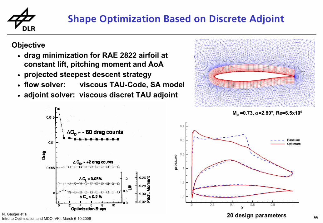
Shape Optimization Based on Discrete AdjointObjective
• drag minimization for RAE 2822 airfoil atconstant lift, pitching moment and AoA
• projected steepest descent strategy • flow solver: viscous TAU-Code, SA model• adjoint solver: viscous discret TAU adjoint
20 design parameters
M∞ =0.73, α=2.80°, Re=6.5x10⁶
Shape Optimization Based on Discrete Adjoint
67N. Gauger et al.Intro to Optimization and MDO, VKI, March 6-10,2006
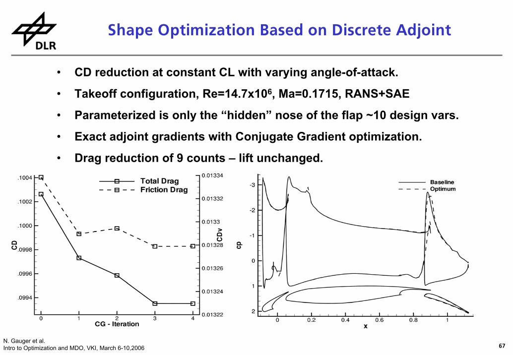
• CD reduction at constant CL with varying angle-of-attack.
• Takeoff configuration, Re=14.7x10⁶, Ma=0.1715, RANS+SAE
• Parameterized is only the “hidden” nose of the flap ~10 design vars.
• Exact adjoint gradients with Conjugate Gradient optimization.
• Drag reduction of 9 counts – lift unchanged.
Shape Optimization Based on Discrete Adjoint
68N. Gauger et al.Intro to Optimization and MDO, VKI, March 6-10,2006
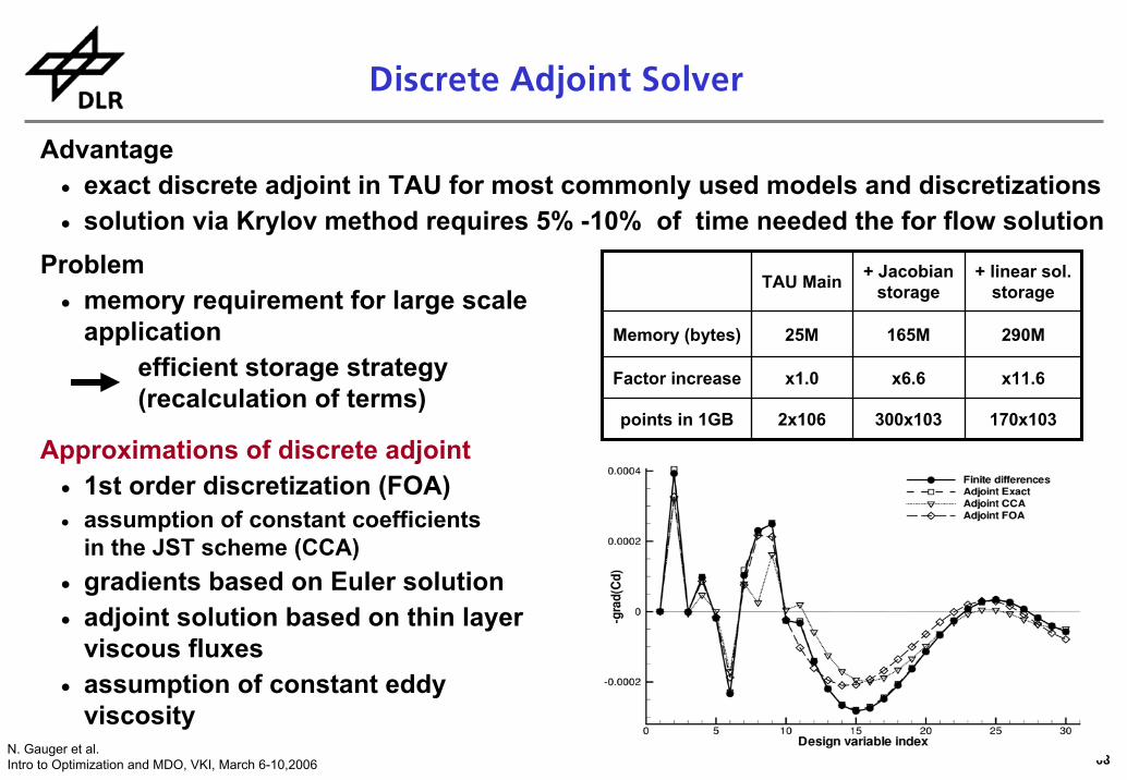
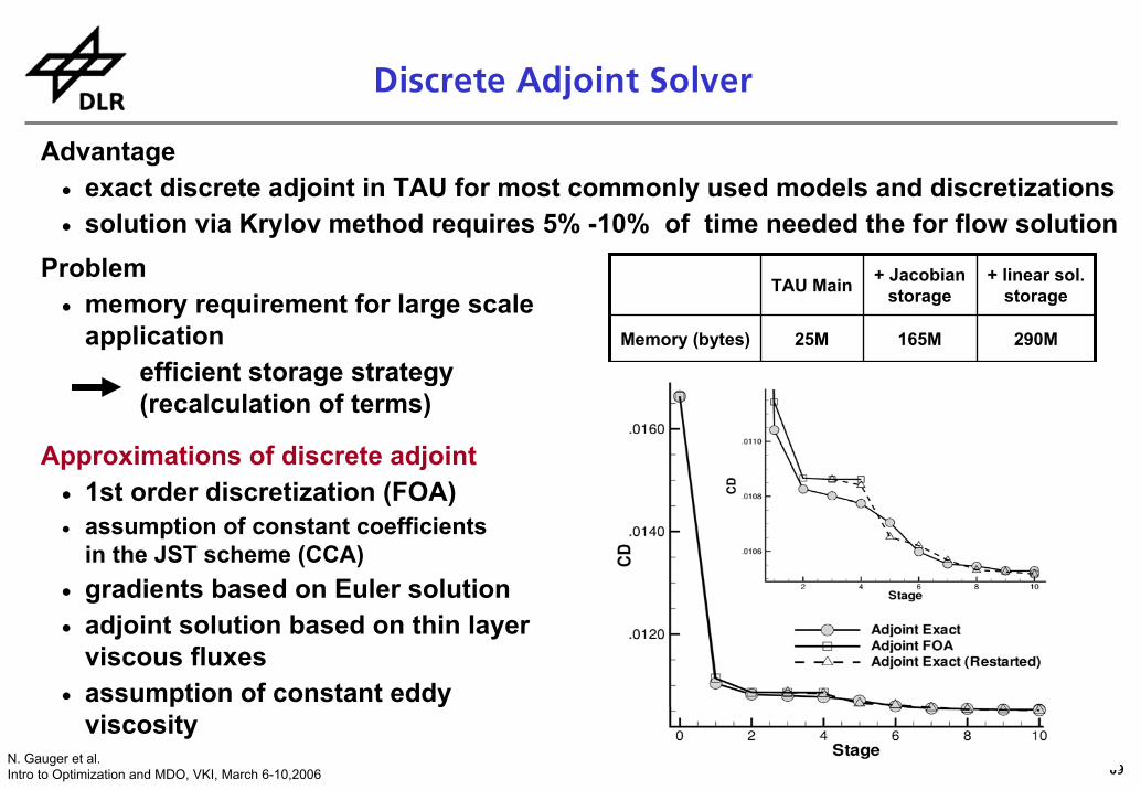
Discrete Adjoint Solver
Advantage• exact discrete adjoint in TAU for most commonly used models and discretizations• solution via Krylov method requires 5% -10% of time needed the for flow solution
Problem• memory requirement for large scale
application efficient storage strategy(recalculation of terms)
TAU Main + Jacobianstorage
+ linear sol.storage
Memory (bytes) 25M 165M 290M
Factor increase x1.0 x6.6 x11.6
points in 1GB 2x10⁶ 300x103 170x103
Approximations of discrete adjoint• 1st order discretization (FOA)• assumption of constant coefficients
in the JST scheme (CCA)• gradients based on Euler solution• adjoint solution based on thin layer
viscous fluxes• assumption of constant eddy
viscosity
Discrete Adjoint Solver
69N. Gauger et al.Intro to Optimization and MDO, VKI, March 6-10,2006
Discrete Adjoint Solver
Advantage• exact discrete adjoint in TAU for most commonly used models and discretizations• solution via Krylov method requires 5% -10% of time needed the for flow solution
Problem• memory requirement for large scale
application efficient storage strategy(recalculation of terms)
TAU Main + Jacobianstorage
+ linear sol.storage
Memory (bytes) 25M 165M 290M
Factor increase x1.0 x6.6 x11.6
points in 1GB 2x10⁶ 300x103 170x103
Approximations of discrete adjoint• 1st order discretization (FOA)• assumption of constant coefficients
in the JST scheme (CCA)• gradients based on Euler solution• adjoint solution based on thin layer
viscous fluxes• assumption of constant eddy
viscosity
Discrete Adjoint Solver
70N. Gauger et al.Intro to Optimization and MDO, VKI, March 6-10,2006
Algorithmic Differentiation (AD)
Work in progress and results
• ADFLOWer generated with TAF (3D Navier-Stokes,k-w), first verifications and validation
• Adjoint version of TAUij (2D Euler) + mesh deformationand parameterization with ADOL-C, validated versus finite differences and first applications
• First and second derivatives of a “FLOWer-Derivate”(2D Euler) + mesh deformation and parameterizationgenerated with TAPENADE, used for One Shot (Piggy Back)
71N. Gauger et al.Intro to Optimization and MDO, VKI, March 6-10,2006
72N. Gauger et al.Intro to Optimization and MDO, VKI, March 6-10,2006

73N. Gauger et al.Intro to Optimization and MDO, VKI, March 6-10,2006
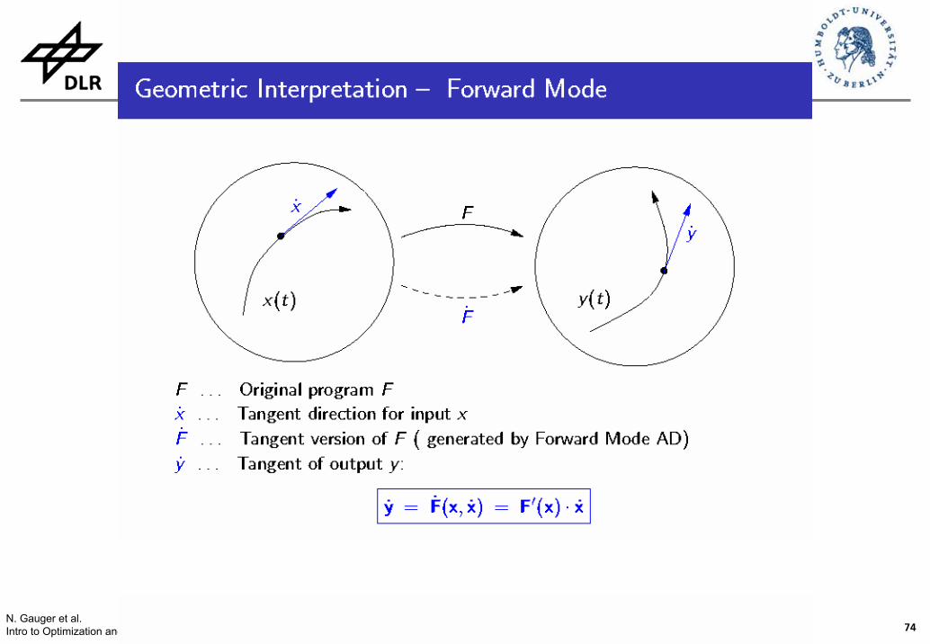
Evaluation of Simple Example:
Simple Example
74N. Gauger et al.Intro to Optimization and MDO, VKI, March 6-10,2006
75N. Gauger et al.Intro to Optimization and MDO, VKI, March 6-10,2006
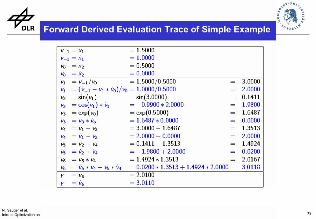
Forward Derived Evaluation Trace of Simple Example
76N. Gauger et al.Intro to Optimization and MDO, VKI, March 6-10,2006
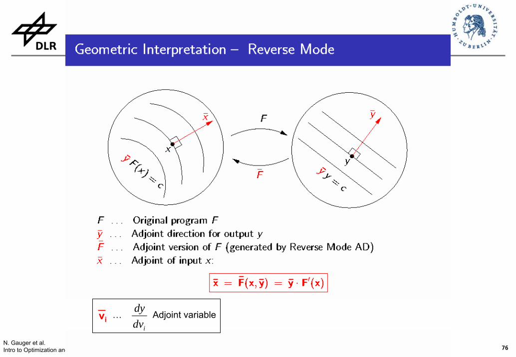
idvdy
vi … Adjoint variable
77N. Gauger et al.Intro to Optimization and MDO, VKI, March 6-10,2006
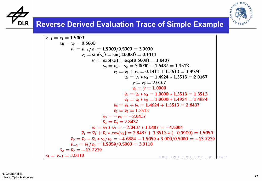
Reverse Derived Evaluation Trace of Simple Example
78N. Gauger et al.Intro to Optimization and MDO, VKI, March 6-10,2006
FastOpt
Test configuration2d NACA12k-omega (Wilcox) turbulence modelcell-centred metric2 time steps on fine gridtarget sensitivity: d lift/ d alpha
StepsModifications of FLOWer code (TAF Directives, slight recoding, etc...)tangent-linear code (verification + useful per se small dimensional design problems) adjoint codeeifficient adjoint code
Major challengememory management (all variables in one big field 'variab')complicates detailed analysis and handling of deallocation
ADFLOWer by TAF
79N. Gauger et al.Intro to Optimization and MDO, VKI, March 6-10,2006
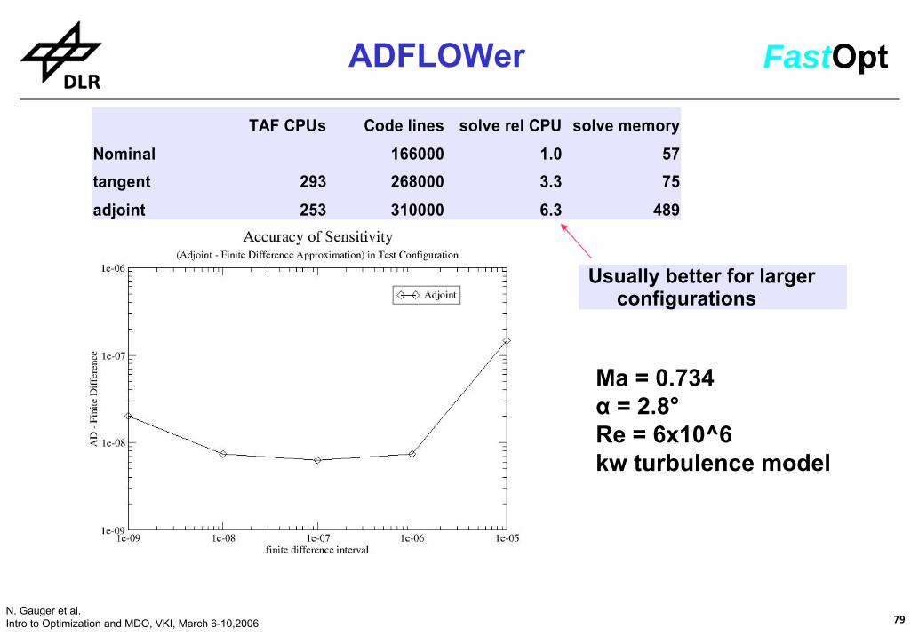
TAF CPUs Code lines solve rel CPU solve memoryNominal 166000 1.0 57tangent 293 268000 3.3 75adjoint 253 310000 6.3 489
Usually better for larger configurations
Ma = 0.734α = 2.8°Re = 6x10^6kw turbulence model
ADFLOWer FastOpt
80N. Gauger et al.Intro to Optimization and MDO, VKI, March 6-10,2006
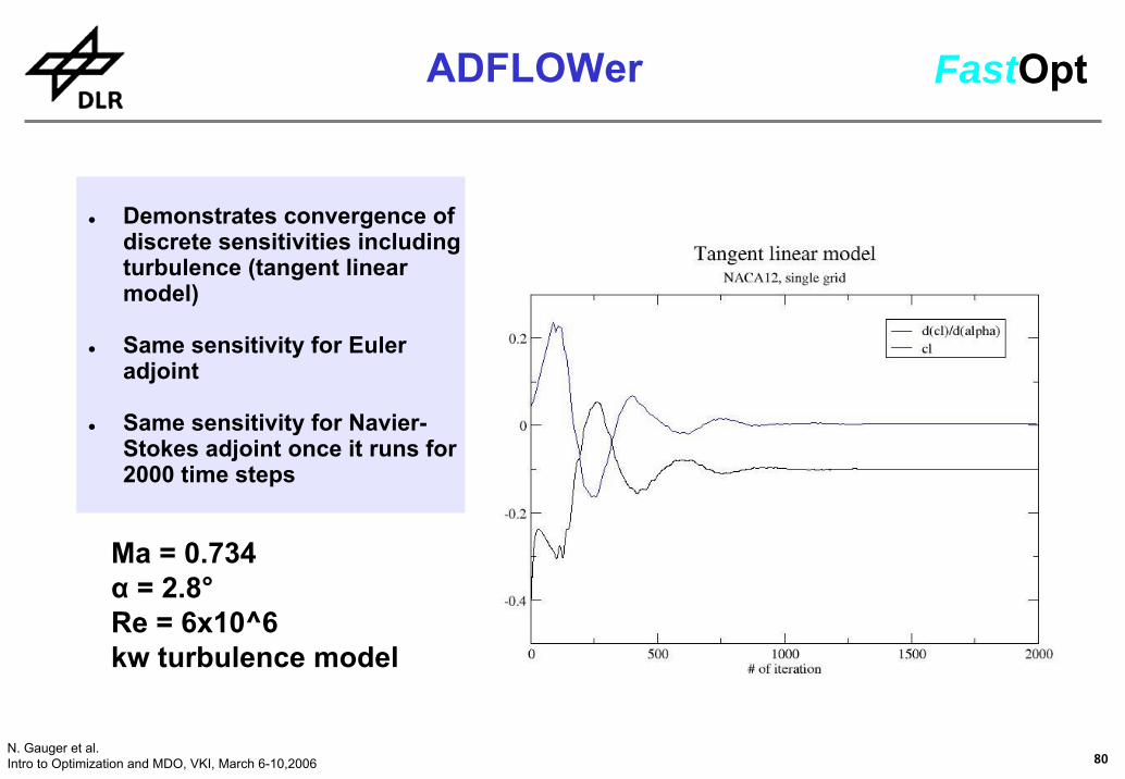
Demonstrates convergence of discrete sensitivities including turbulence (tangent linear model)
Same sensitivity for Euler adjoint
Same sensitivity for Navier-Stokes adjoint once it runs for 2000 time steps
Ma = 0.734α = 2.8°Re = 6x10^6kw turbulence model
ADFLOWer FastOpt
81N. Gauger et al.Intro to Optimization and MDO, VKI, March 6-10,2006
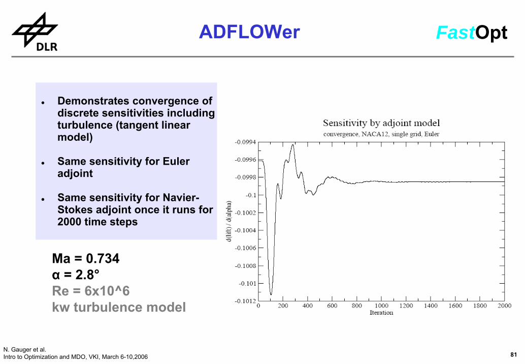
Demonstrates convergence of discrete sensitivities including turbulence (tangent linear model)
Same sensitivity for Euler adjoint
Same sensitivity for Navier-Stokes adjoint once it runs for 2000 time steps
Ma = 0.734α = 2.8°Re = 6x10^6kw turbulence model
ADFLOWer FastOpt
82N. Gauger et al.Intro to Optimization and MDO, VKI, March 6-10,2006
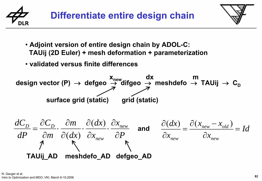
Differentiate entire design chain
• Adjoint version of entire design chain by ADOL-C:TAUij (2D Euler) + mesh deformation + parameterization
• validated versus finite differences
design vector (P) → defgeo → difgeo → meshdefo → TAUij → CDxnew dx m
surface grid (static) grid (static)
Px
xdx
dxm
mC
dPdC new
new
DD
∂∂
⋅∂∂
⋅∂∂
⋅∂
∂=
)()(
Idx
xxxdx
new
oldnew
new
=∂
−∂=
∂∂ )()(
and
TAUij_AD meshdefo_AD defgeo_AD
83N. Gauger et al.Intro to Optimization and MDO, VKI, March 6-10,2006
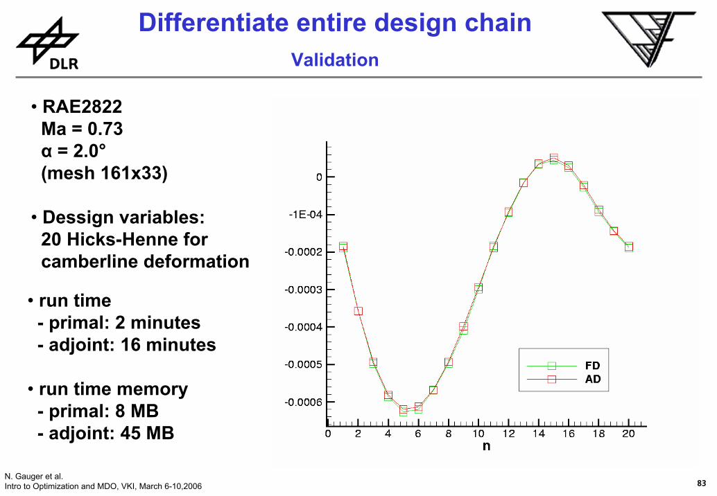
• RAE2822Ma = 0.73α = 2.0°(mesh 161x33)
• Dessign variables:20 Hicks-Henne forcamberline deformation
• run time- primal: 2 minutes- adjoint: 16 minutes
• run time memory- primal: 8 MB- adjoint: 45 MB
Differentiate entire design chainValidation
84N. Gauger et al.Intro to Optimization and MDO, VKI, March 6-10,2006
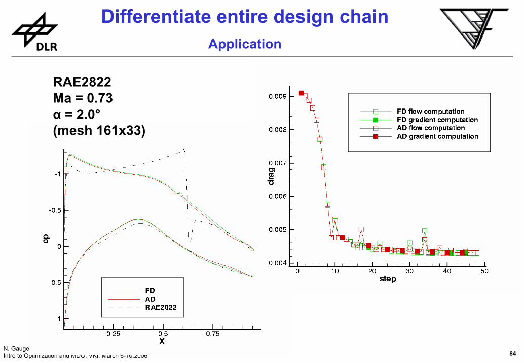
Differentiate entire design chainApplication
RAE2822Ma = 0.73α = 2.0°(mesh 161x33)
85N. Gauger et al.Intro to Optimization and MDO, VKI, March 6-10,2006
• Continuous Adjoint- optimize then discretize- hand coded adjoint solvers- time consuming in implementation- efficient in run and memory
• Discrete Adjoint / Algorithmic Differentiation (AD)- discretize then optimize- hand coding of adjoint solvers or …- … more or less automated generation- memory effort increases (way out e.g. check-pointing)
• Hybrid Adjoint- use source to source AD tools - optimize differentiated code- merge “continuous and discrete” routines
Different adjoint approaches
86N. Gauger et al.Intro to Optimization and MDO, VKI, March 6-10,2006
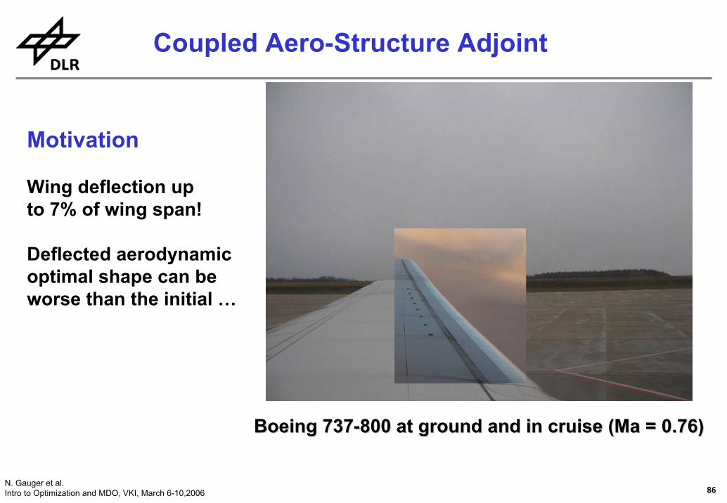
Coupled Aero-Structure Adjoint
Motivation
Wing deflection up to 7% of wing span!
Deflected aerodynamicoptimal shape can beworse than the initial …
Boeing 737Boeing 737--800 at ground and in cruise (Ma = 0.76)800 at ground and in cruise (Ma = 0.76)
87N. Gauger et al.Intro to Optimization and MDO, VKI, March 6-10,2006
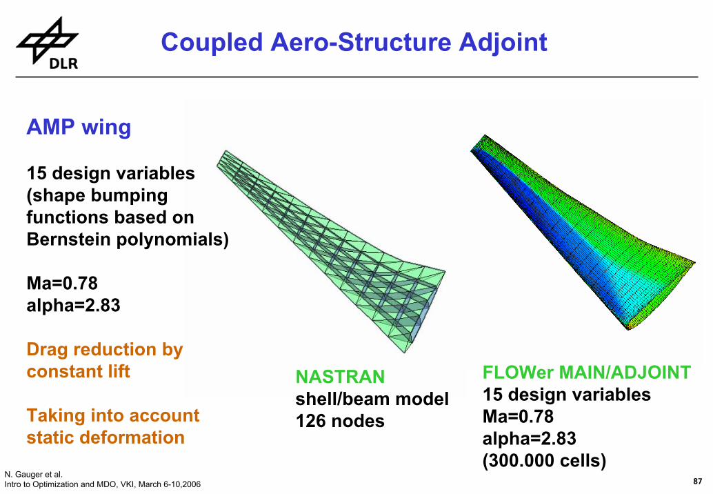
Coupled Aero-Structure Adjoint
AMP wing
15 design variables(shape bumping functions based on Bernstein polynomials)
Ma=0.78alpha=2.83
Drag reduction byconstant lift
Taking into accountstatic deformation
NASTRANshell/beam model126 nodes
FLOWer MAIN/ADJOINT15 design variablesMa=0.78alpha=2.83(300.000 cells)
88N. Gauger et al.Intro to Optimization and MDO, VKI, March 6-10,2006
A
TAD
S
TS
dR
dC
dR ψψ ~⎟
⎠⎞
⎜⎝⎛
∂∂
−∂
∂=⎟
⎠⎞
⎜⎝⎛
∂∂
Pd
dC
Pw
wC
PC
dPdC DDDD
∂∂
∂∂
+∂∂
∂∂
+∂
∂=
PR
PR
PC
dPdC ST
SAT
ADD
∂∂
−∂∂
−∂
∂= ψψ
S
TSD
A
TA
wR
wC
wR ψψ ~⎟
⎠⎞
⎜⎝⎛
∂∂
−∂
∂=⎟
⎠⎞
⎜⎝⎛
∂∂
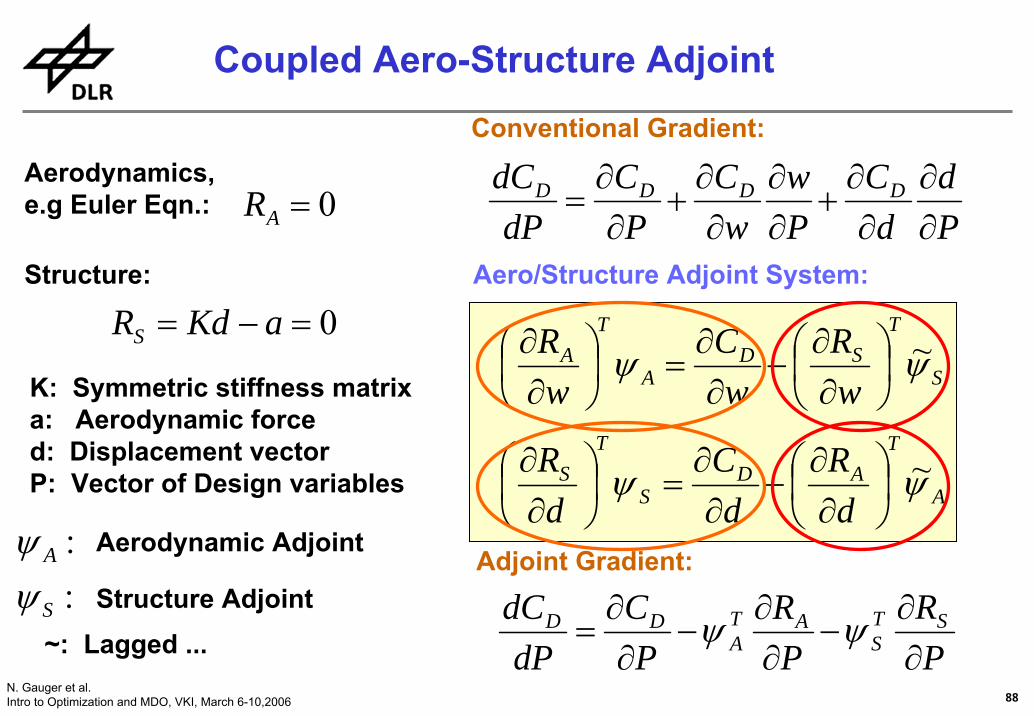
0=AR
0=−= aKdRS
Structure:
Aerodynamics, e.g Euler Eqn.:
K: Symmetric stiffness matrixa: Aerodynamic forced: Displacement vectorP: Vector of Design variables
Coupled Aero-Structure Adjoint
Adjoint Gradient:
Aero/Structure Adjoint System:
Conventional Gradient:
::
S
A
ψψ Aerodynamic Adjoint
Structure Adjoint~: Lagged ...
89N. Gauger et al.Intro to Optimization and MDO, VKI, March 6-10,2006
Coupled Aero-Structure Adjoint
Pad
PK
PaKd
PR
KKd
aKddR
wa
waKd
wR
wC
PC
dC
PR
dR
S
TS
S
D
DD
AA
∂∂
−∂∂
=∂
−∂=
∂∂
==∂
−∂=
∂∂
∂∂
−=∂
−∂=
∂∂
∂∂
∂∂
∂∂
∂∂
∂∂
)(
)(
)(
,
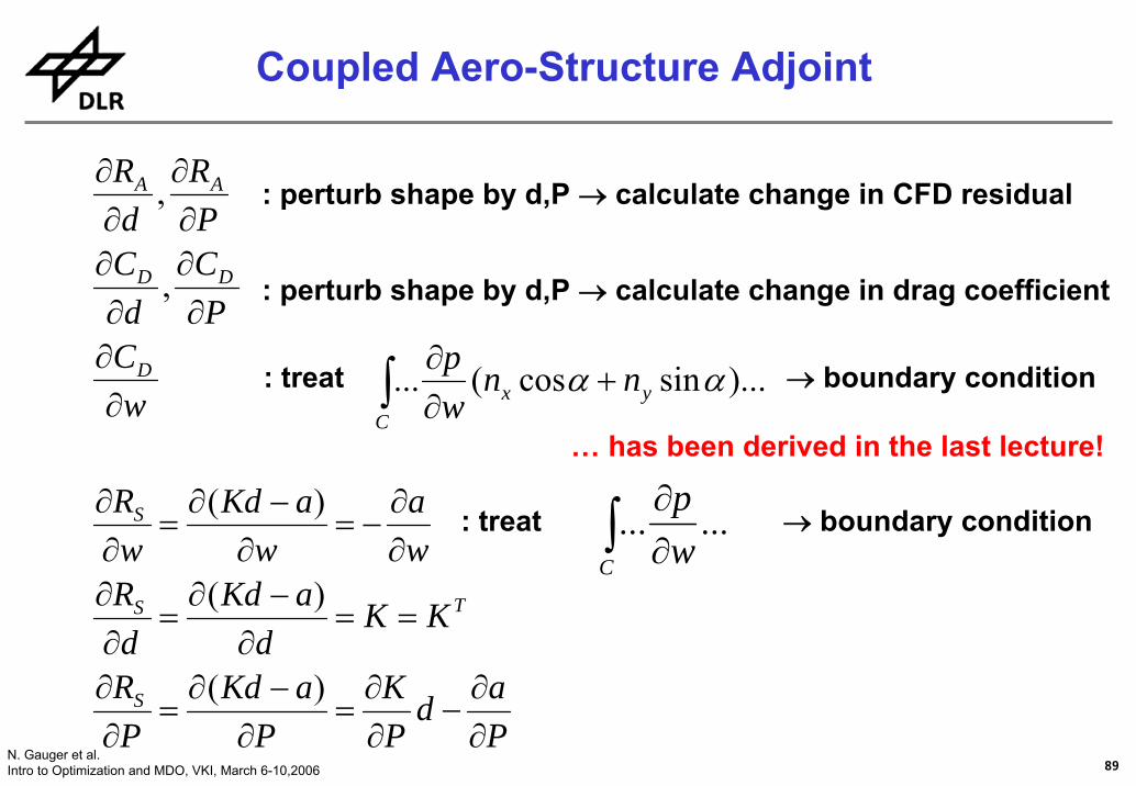
, : perturb shape by d,P → calculate change in CFD residual
: perturb shape by d,P → calculate change in drag coefficient
: treat → boundary condition∫ +∂∂
Cyx nn
wp )...sincos(... αα
: treat → boundary condition∫ ∂∂
C wp ......
… has been derived in the last lecture!
90N. Gauger et al.Intro to Optimization and MDO, VKI, March 6-10,2006
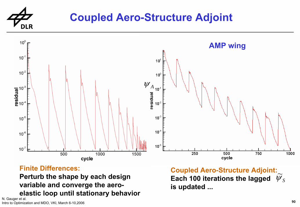
Coupled Aero-Structure Adjoint
Finite Differences:Perturb the shape by each designvariable and converge the aero-elastic loop until stationary behavior
Coupled Aero-Structure Adjoint:Each 100 iterations the laggedis updated ...
Sψ~
AMP wing
Aψ
91N. Gauger et al.Intro to Optimization and MDO, VKI, March 6-10,2006
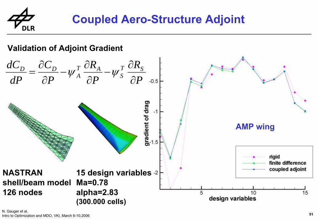
PR
PR
PC
dPdC ST
SAT
ADD
∂∂
−∂∂
−∂
∂= ψψ
Validation of Adjoint Gradient
NASTRANshell/beam model126 nodes
15 design variablesMa=0.78alpha=2.83(300.000 cells)
AMP wing
Coupled Aero-Structure Adjoint
92N. Gauger et al.Intro to Optimization and MDO, VKI, March 6-10,2006
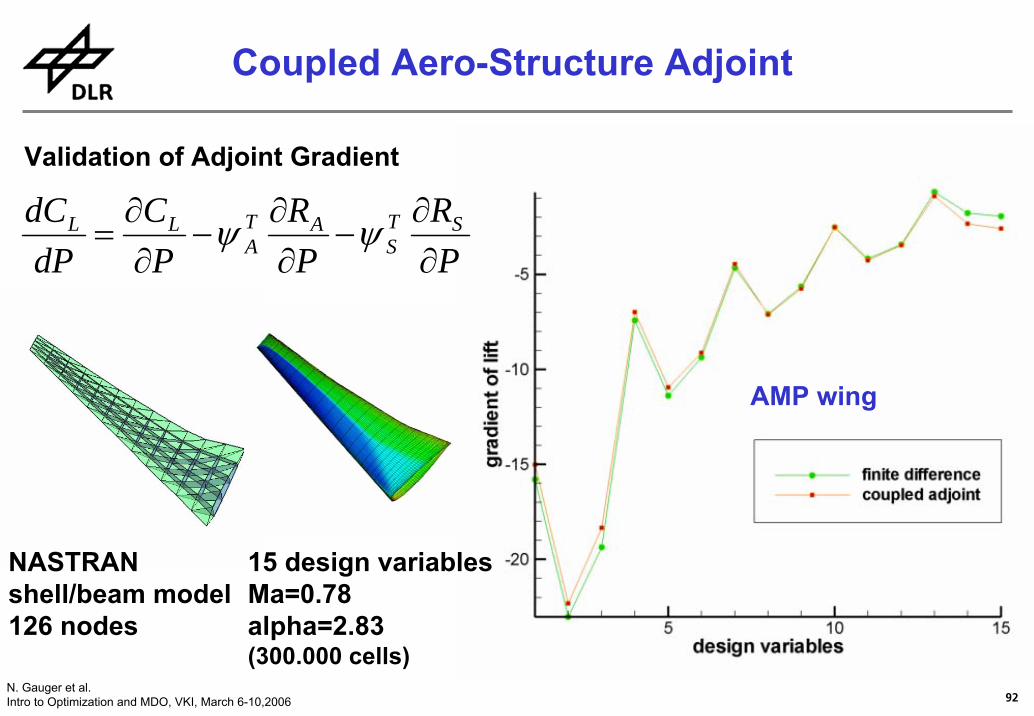
PR
PR
PC
dPdC ST
SAT
ALL
∂∂
−∂∂
−∂
∂= ψψ
Validation of Adjoint Gradient
NASTRANshell/beam model126 nodes
15 design variablesMa=0.78alpha=2.83(300.000 cells)
AMP wing
Coupled Aero-Structure Adjoint
93N. Gauger et al.Intro to Optimization and MDO, VKI, March 6-10,2006
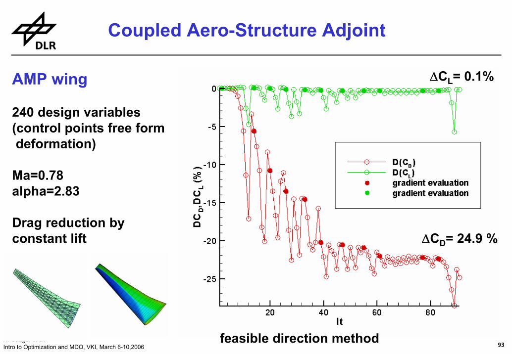
Coupled Aero-Structure Adjoint
AMP wing
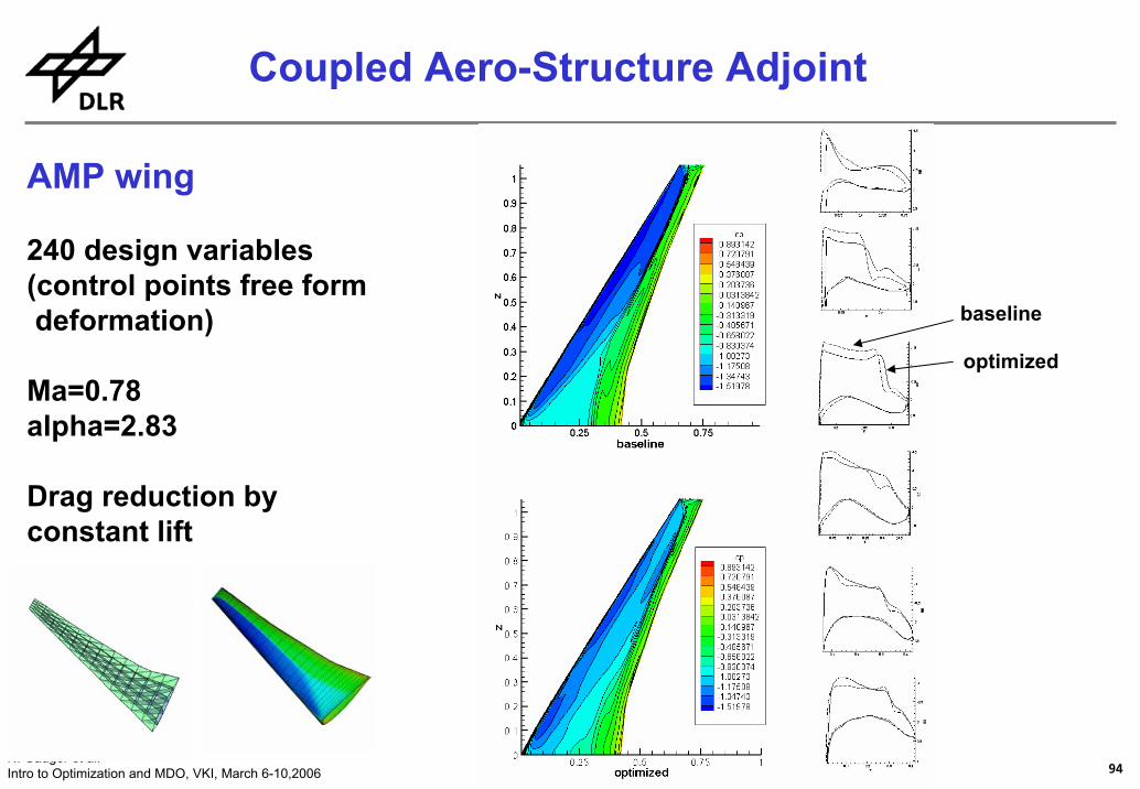
240 design variables(control points free form deformation)
Ma=0.78alpha=2.83
Drag reduction byconstant lift ΔCD= 24.9 %
ΔCL= 0.1%
feasible direction method
94N. Gauger et al.Intro to Optimization and MDO, VKI, March 6-10,2006
Coupled Aero-Structure Adjoint
AMP wing
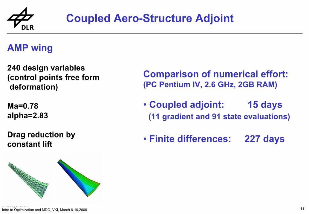
240 design variables(control points free form deformation)
Ma=0.78alpha=2.83
Drag reduction byconstant lift
baseline
optimized
95N. Gauger et al.Intro to Optimization and MDO, VKI, March 6-10,2006
Coupled Aero-Structure Adjoint
Comparison of numerical effort:(PC Pentium IV, 2.6 GHz, 2GB RAM)
• Coupled adjoint: 15 days(11 gradient and 91 state evaluations)
• Finite differences: 227 days
AMP wing
240 design variables(control points free form deformation)
Ma=0.78alpha=2.83
Drag reduction byconstant lift
96N. Gauger et al.Intro to Optimization and MDO, VKI, March 6-10,2006
Aero-Structure MDO
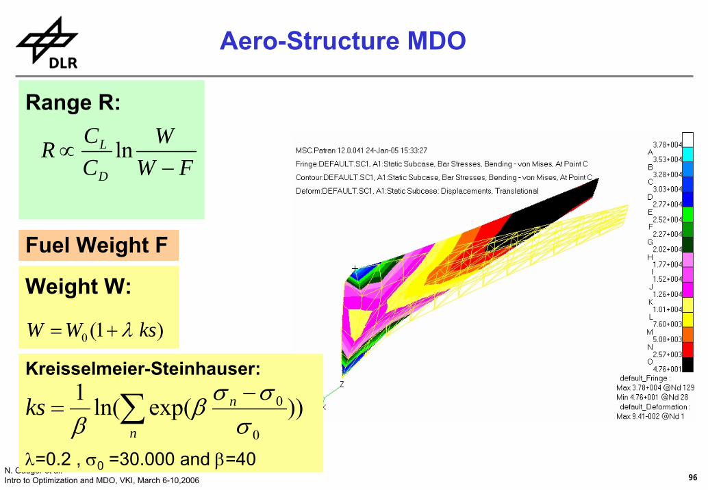
FWW
CCR
D
L
−∝ ln
)1(0 ksWW λ+=
∑ −=
n
nks ))exp(ln(1
0
0
σσσβ
βλ=0.2 , σ0 =30.000 and β=40
Range R:
Weight W:
Fuel Weight F
Kreisselmeier-Steinhauser:
97N. Gauger et al.Intro to Optimization and MDO, VKI, March 6-10,2006
Aero-Structure MDO
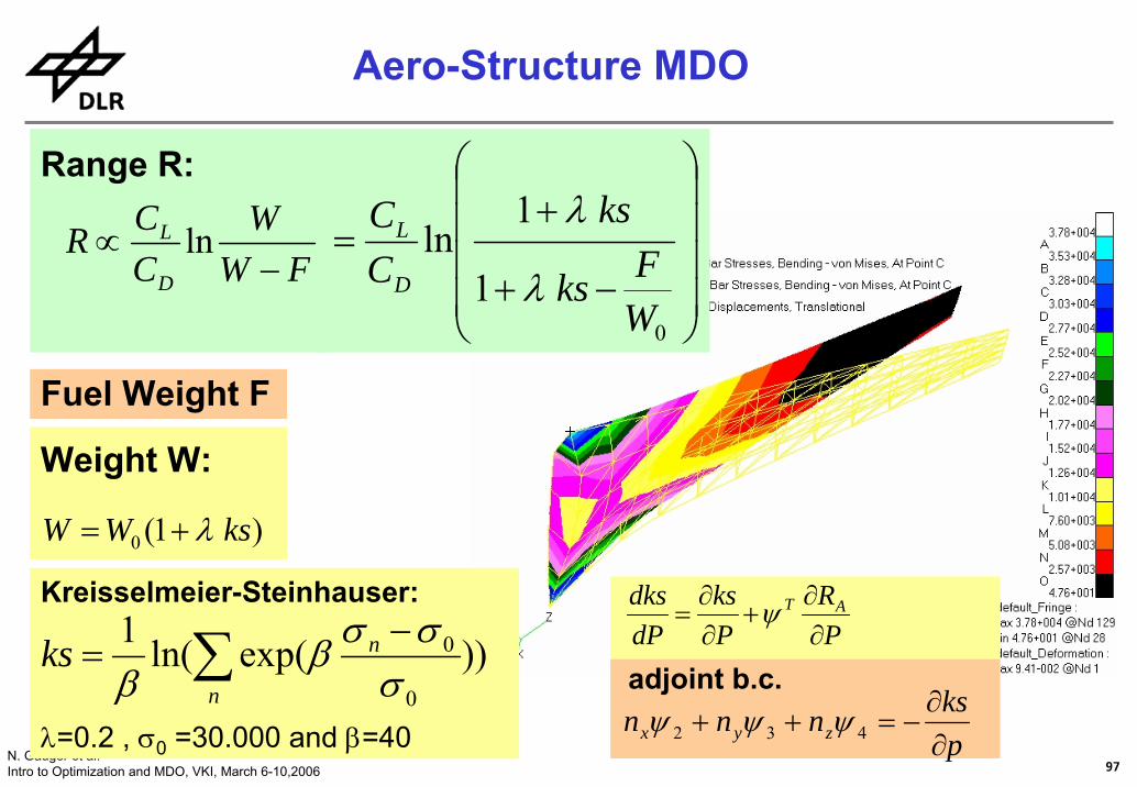
FWW
CCR
D
L
−∝ ln
)1(0 ksWW λ+=
∑ −=
n
nks ))exp(ln(1
0
0
σσσβ
βλ=0.2 , σ0 =30.000 and β=40
Range R:
Weight W:
Fuel Weight F
⎟⎟⎟⎟
⎠
⎞
⎜⎜⎜⎜
⎝
⎛
−+
+=
0
1
1ln
WFks
ksCC
D
L
λ
λ
Kreisselmeier-Steinhauser:PR
Pks
dPdks AT
∂∂
+∂∂
= ψ
pksnnn zyx ∂
∂−=++ 432 ψψψ
adjoint b.c.
98N. Gauger et al.Intro to Optimization and MDO, VKI, March 6-10,2006
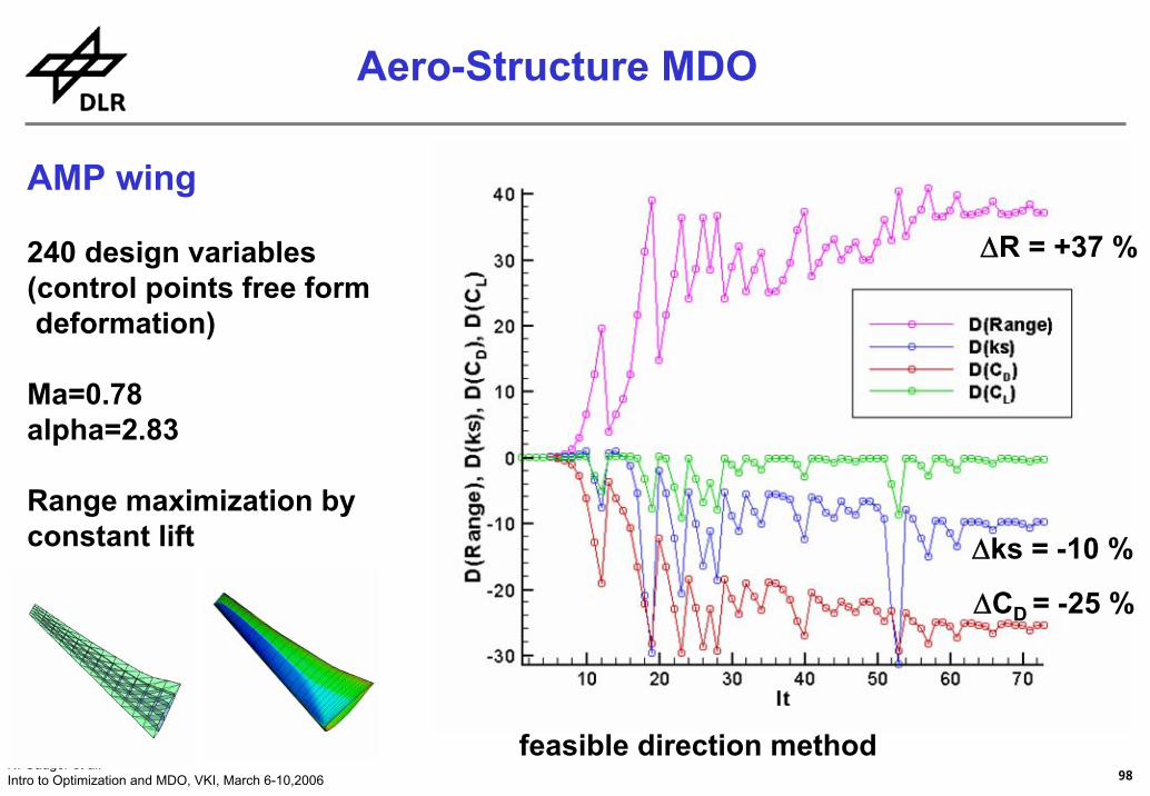
AMP wing
240 design variables(control points free form deformation)
Ma=0.78alpha=2.83
Range maximization byconstant lift
Aero-Structure MDO
ΔCD = -25 %
Δks = -10 %
ΔR = +37 %
feasible direction method
99N. Gauger et al.Intro to Optimization and MDO, VKI, March 6-10,2006
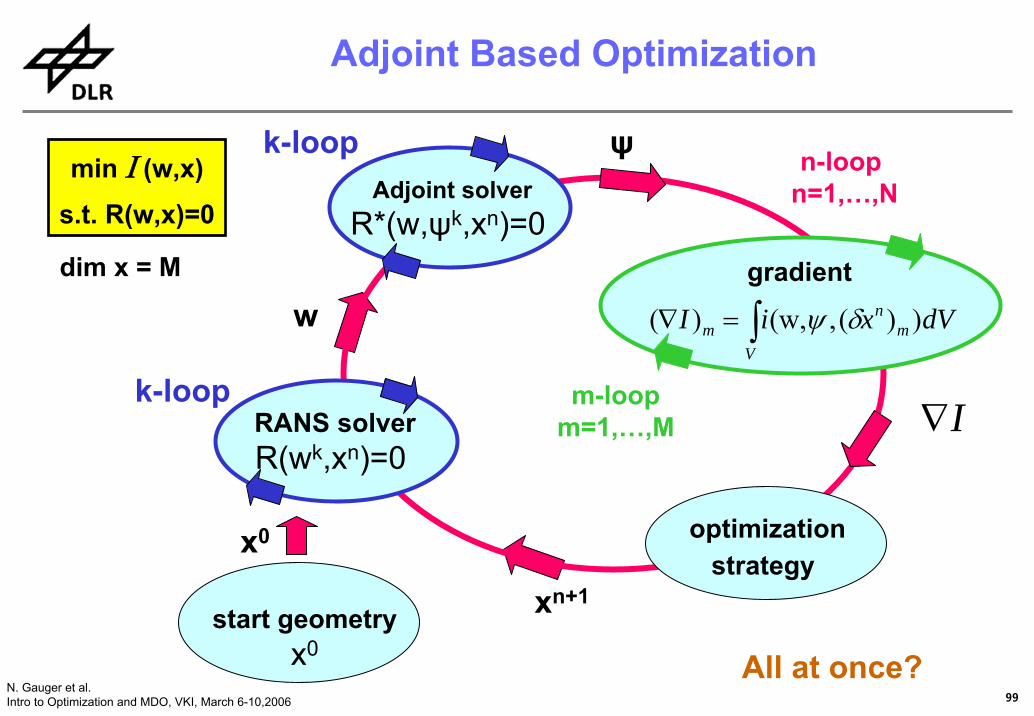
I∇
start geometryx0
ψ
x0
w
xn+1
k-loop
k-loop
Adjoint Based Optimization
min Ι (w,x)s.t. R(w,x)=0
optimizationstrategy
RANS solverR(wk,xn)=0
gradient
∫=∇V
mn
m dVxiI ))(,(w,)( δψ
Adjoint solverR*(w,ψk,xn)=0
dim x = M
n-loop n=1,…,N
m-loopm=1,…,M
All at once?
100N. Gauger et al.Intro to Optimization and MDO, VKI, March 6-10,2006
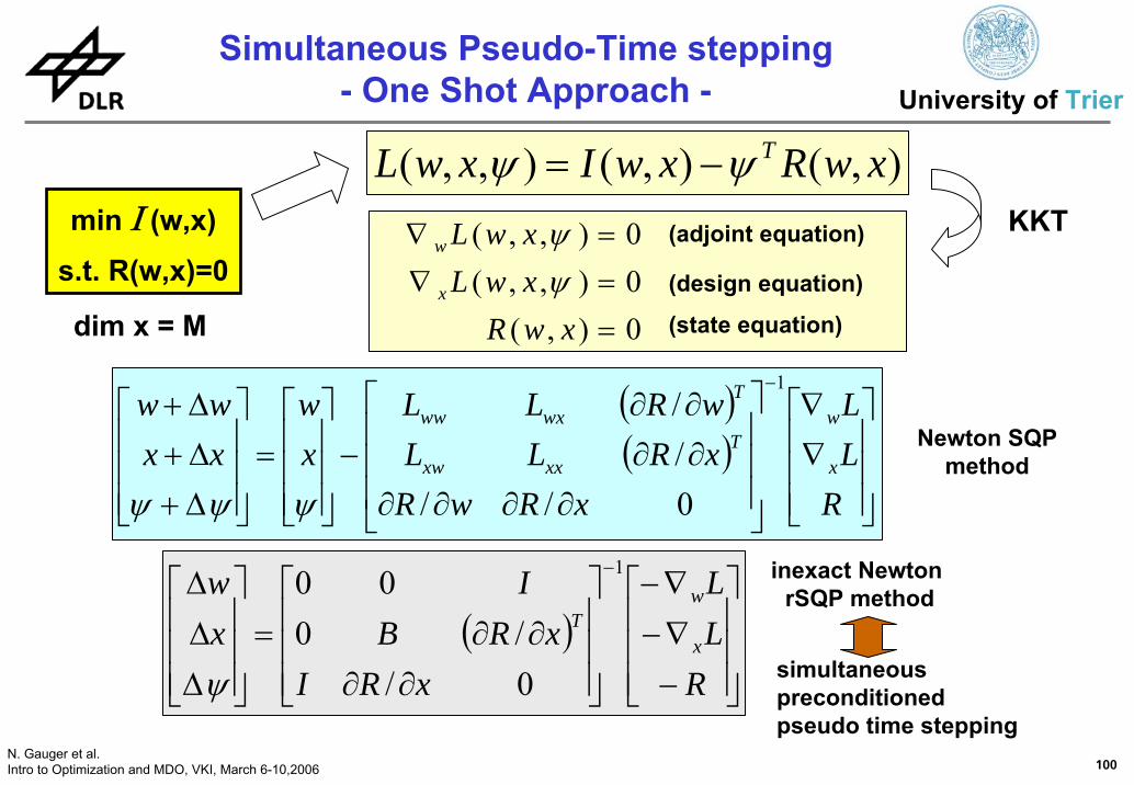
),(),(),,( xwRxwIxwL Tψψ −=
Simultaneous Pseudo-Time stepping- One Shot Approach -
0),(0),,(0),,(
==∇=∇
xwRxwLxwL
x
w
ψψ
(state equation)
(adjoint equation)
(design equation)
University of Trier
min Ι (w,x)
s.t. R(w,x)=0
dim x = M
( )( )
⎥⎥⎥
⎦
⎤
⎢⎢⎢
⎣
⎡∇∇
⎥⎥⎥
⎦
⎤
⎢⎢⎢
⎣
⎡
∂∂∂∂∂∂∂∂
−⎥⎥⎥
⎦
⎤
⎢⎢⎢
⎣
⎡=
⎥⎥⎥
⎦
⎤
⎢⎢⎢
⎣
⎡
Δ+Δ+Δ+
−
RLL
xRwRxRLLwRLL
xw
xxww
x
wT
xxxw
Twxww
1
0////
ψψψ
( )⎥⎥⎥
⎦
⎤
⎢⎢⎢
⎣
⎡
−∇−∇−
⎥⎥⎥
⎦
⎤
⎢⎢⎢
⎣
⎡
∂∂∂∂=
⎥⎥⎥
⎦
⎤
⎢⎢⎢
⎣
⎡
ΔΔΔ −
RLL
xRIxRB
Ixw
x
wT
1
0//0
00
ψ
KKT
Newton SQPmethod
inexact Newton rSQP method
simultaneous preconditionedpseudo time stepping
101N. Gauger et al.Intro to Optimization and MDO, VKI, March 6-10,2006
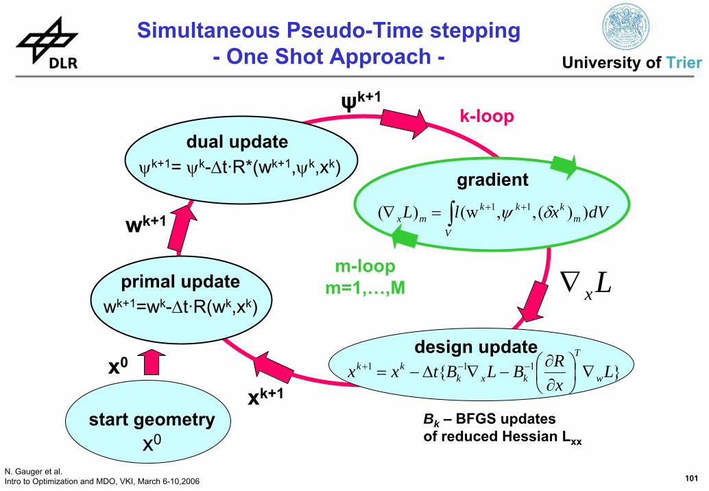
Lx∇
start geometryx0
ψk+1
x0
wk+1
xk+1
primal updatewk+1=wk-Δt·R(wk,xk)
gradient
∫ ++=∇V
mkkk
mx dVxlL ))(,,(w)( 11 δψ
k-loop dual update
ψk+1= ψk-Δt·R*(wk+1,ψk,xk)
}{ 111 LxRBLBtxx w
T
kxkkk ∇⎟
⎠⎞
⎜⎝⎛
∂∂
−∇Δ−= −−+
m-loopm=1,…,M
design update
Bk – BFGS updatesof reduced Hessian Lxx
Simultaneous Pseudo-Time stepping- One Shot Approach - University of Trier
102N. Gauger et al.Intro to Optimization and MDO, VKI, March 6-10,2006
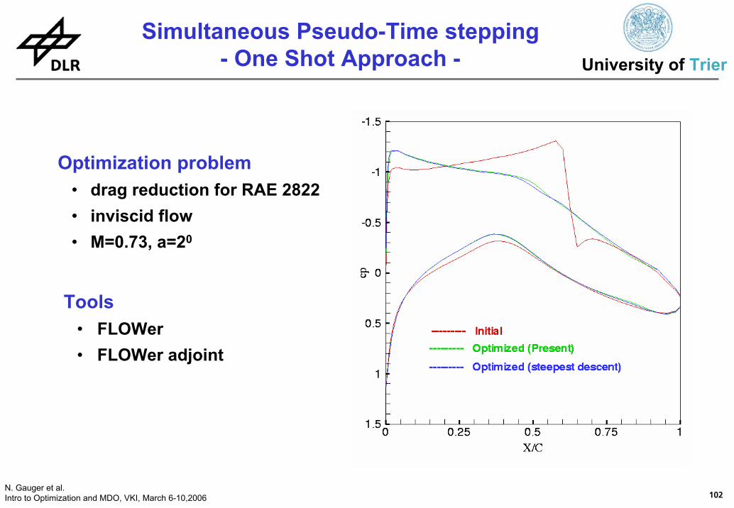
Optimization problem• drag reduction for RAE 2822 • inviscid flow• M=0.73, a=20
Tools• FLOWer• FLOWer adjoint
Simultaneous Pseudo-Time stepping- One Shot Approach - University of Trier
103N. Gauger et al.Intro to Optimization and MDO, VKI, March 6-10,2006
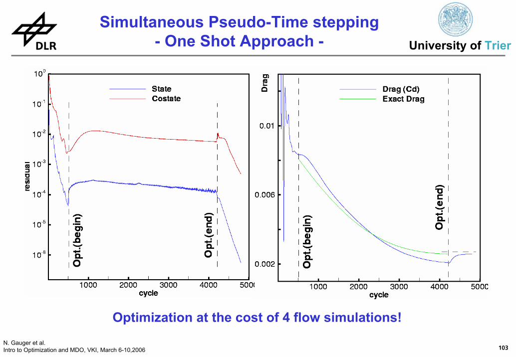
Optimization at the cost of 4 flow simulations!
Simultaneous Pseudo-Time stepping- One Shot Approach - University of Trier
104N. Gauger et al.Intro to Optimization and MDO, VKI, March 6-10,2006
Optimal Design ScenarioPiggy–Back Approach
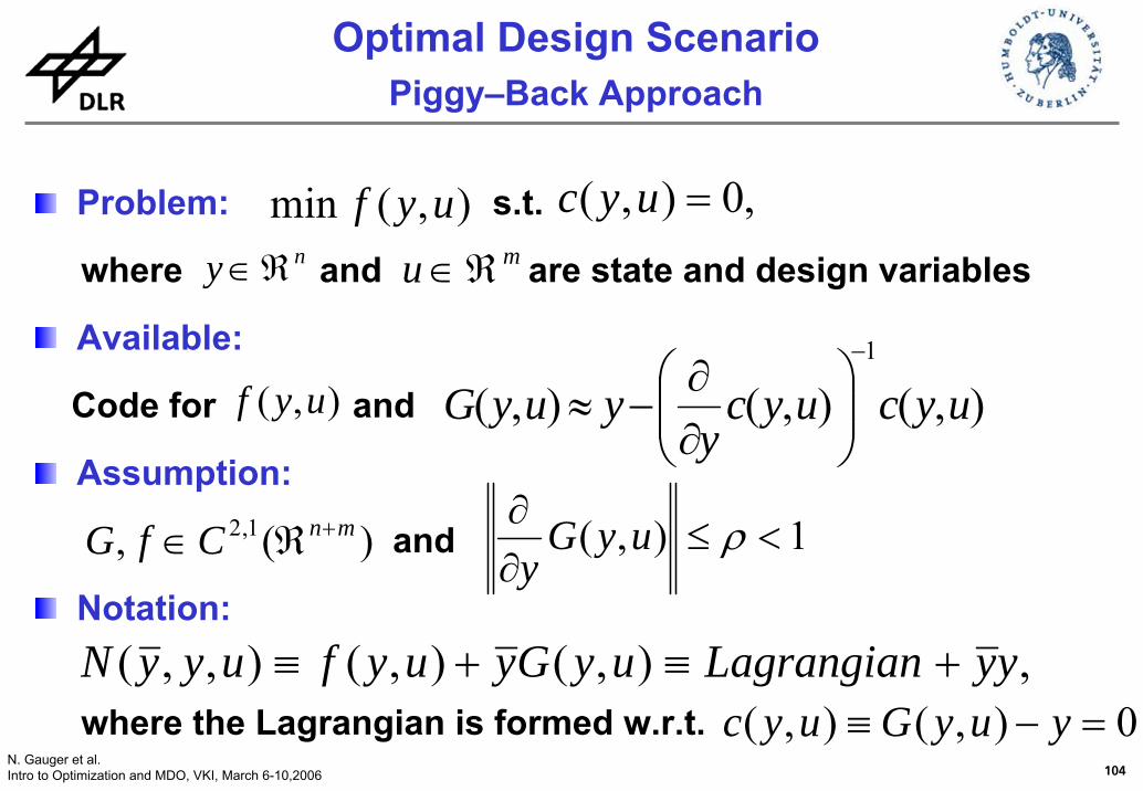
Problem: s.t.
where and are state and design variables
Available:
Code for and
Assumption:
and
Notation:
where the Lagrangian is formed w.r.t.
),(min uyf ,0),( =uycny ℜ∈ mu ℜ∈
),( uyf ),(),(),(1
uycuycy
yuyG−
⎟⎟⎠
⎞⎜⎜⎝
⎛∂∂
−≈
)(, 1,2 mnCfG +ℜ∈ 1),( <≤∂∂ ρuyGy
,),(),(),,( yyLagrangianuyGyuyfuyyN +≡+≡0),(),( =−≡ yuyGuyc
105N. Gauger et al.Intro to Optimization and MDO, VKI, March 6-10,2006
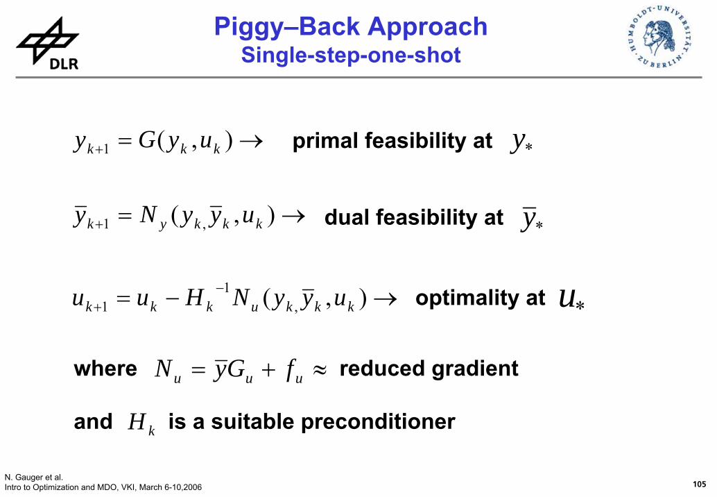
Piggy–Back ApproachSingle-step-one-shot
→−=
→=
→=
−+
+
+
),(
),(
),(
,1
1
,1
1
kkkukkk
kkkyk
kkk
uyyNHuu
uyyNy
uyGy primal feasibility at
dual feasibility at
optimality at
*y
*y
*u
where reduced gradient
and is a suitable preconditioner
≈+= uuu fGyN
kH
106N. Gauger et al.Intro to Optimization and MDO, VKI, March 6-10,2006
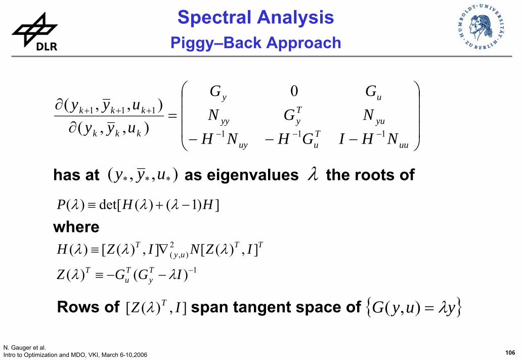
Spectral AnalysisPiggy–Back Approach
⎟⎟⎟
⎠
⎞
⎜⎜⎜
⎝
⎛
−−−=
∂∂
−−−
+++
uuTuuy
yuTyyy
uy
kkk
kkk
NHIGHNHNGNGG
uyyuyy
111
111
0
),,(),,(
1
2),(
)()(
],)([],)([)(
])1()(det[)(
−−−≡
∇≡
−+≡
IGGZ
IZNIZH
HHP
Ty
Tu
T
TTuy
T
λλ
λλλ
λλλ
has at as eigenvalues the roots of ),,( *** uyy
where
λ
Rows of span tangent space of],)([ IZ Tλ { }yuyG λ=),(
107N. Gauger et al.Intro to Optimization and MDO, VKI, March 6-10,2006
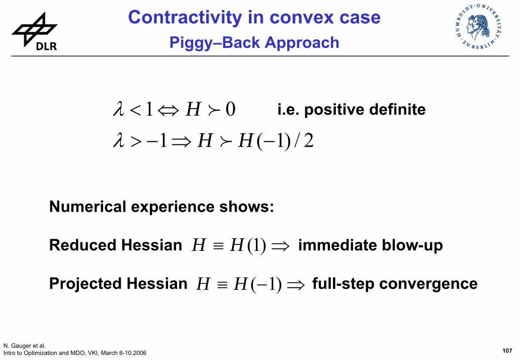
Contractivity in convex casePiggy–Back Approach
2/)1(101
−⇒−>⇔<
HHH
f
f
λλ i.e. positive definite
Numerical experience shows:
Reduced Hessian immediate blow-up
Projected Hessian full-step convergence⇒−≡ )1(HH
⇒≡ )1(HH

108N. Gauger et al.Intro to Optimization and MDO, VKI, March 6-10,2006
Transonic case: NACA 0012 at Ma = 0.8 with α = 2°
Cost function: glide ratio
“FLOWer-Derivate” (2D Euler) + mesh deformation +parameterization
First and second derivatives by AD tool TAPENADE
Geometric constraint: constant thickness
Camberline/Thickness decomposition,20 Hicks-Henne coefficients define camberline
Piggy–Back Approach - Application
109N. Gauger et al.Intro to Optimization and MDO, VKI, March 6-10,2006
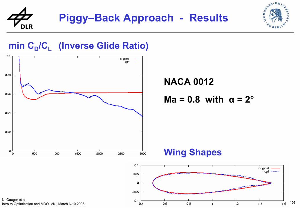
min CD/CL (Inverse Glide Ratio)
Wing Shapes
Piggy–Back Approach - Results
NACA 0012
Ma = 0.8 with α = 2°
110N. Gauger et al.Intro to Optimization and MDO, VKI, March 6-10,2006
Thanks for your attention!


