

AE 549 Linear Stability Theory and
Laminar-Turbulent Transition
Prof. Dr. Serkan ÖZGEN Introduction

Historical Background
Early attempts to understand transition did not care about
turbulence or the details of its initial appearance but tried to
explain why the original laminar flow can not exist indefinetely.
Rayleigh (1880-1913) produced results concerning the
instability of inviscid flows but little progress was made
towards the original goal. The inflectional instability was
discovered by Rayleigh.
Taylor (1915) and Prandtl (1921) indicated that viscosity can
destabilize a flow.
Tollmien (1929) and Schlichting (1935) outlined a complete
theory of boundary-layer stability and calculated the total
amplification of the most unstable frequencies.
2
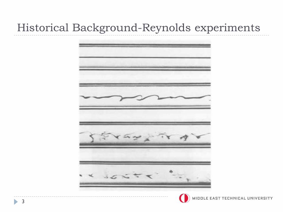
Historical Background-Reynolds experiments
3
Historical Background
Schubauer and Skramstad (1947) performed experiments, which demonstrated the presence of instability waves in a boundary-layer, their connection with transition and the quantitative description of their behavior by the theory of Tollmien and Schlichting.
Smith and Gamberoni (1956) and van Ingen (1956) devised a transition prediction method (en method), which is still widely used today.
Pretsch (1942) provided a large body of numerical results by calculating the stability characteristics of Falkner-Skanvelocity profiles.
In the 1960s, the advent of digital computers permitted solutions to be achieved for many boundary-layer flows like 3-D boundary-layers, compressible boundary-layers, unsteady boundary-layers, etc.
4

Practical Aspects
The problem of understanding the origins of turbulent flow
and transition to turbulent flow are the most important
unsolved problems of fluid mechanics and aerodynamics.
There is a large number of applications for information
regarding transition location and the details of the
subsequent turbulent flow.
5
Practical Aspects
A few examples:
Nose cone and heat shield requirements on reentry vehicles are
critical functions of transition altitude.
If transition can be delayed with laminar flow control on the wings of
large transport aircraft, substantial savings in fuel will result.
Efforts to accurately predict airfoil surface heat transfer and devise a
cooling mechanism for turbine blades are not fully effective due to
absence of a fully reliable transition prediction technique.
Separation and stall on low-Reynolds number airfoils and turbine
blades strongly depend on whether the boundary-layer is laminar,
transitional or turbulent.
The performance and detection of submarines and torpedoes are
influenced by turbulent flows and efforts directed towards drag
reduction require details of the transition process.
6

Practical Aspects
Because of the presence of different factors like disturbance
environment, surface geometry, roughness, heat
transfer, noise level, etc. on transition, it is not possible to
develop general prediction schemes for transition location.
As can be anticipated, no mathematical model exists that can
predict the transition location for a given flow.
7

Basic Concepts of
Hydrodynamic Stability Theory
In order to analyze the stability problem of a laminar flow, one needs to know the velocity, pressure and temperature fields at any point , and time, t, which define the basic flow. The basic flow may be steady or unsteady, but must satisfy the corresponding equations of motion and boundary conditions.
In very simple words, instability occurs because there is a disturbance of the equilibrium of the forces acting on the system, namely external, inertial and viscous forces.
External forces are buoyancy in a fluid of variable density, surface tension, magneto-hydrodynamic forces, centrifugal and coriolisforces.
If a small disturbance is introduced to the flow, it may die out, may preserve its initial amplitude, or it may amplify. Such disturbances are called as stable, neutrally (or marginally) stable or unstable disturbances, respectively.
8
x
Basic Concepts of
Hydrodynamic Stability Theory
Roles of different factors in the stability mechanism:
Gravity: destabilizing if heavier fluid lies on top of lighter fluid,
stabilizing if vice-versa.
Surface tension: tries to decrease the area of a contact surface,
therefore stabilizing.
Viscosity: viscosity has a dual role in the instability mechanism. All
other effects being absent, the onset of instability in a boundary-layer
flow is determined by the relative magnitudes of these two effects.
Viscosity is stabilizing because it dissipates the energy of the
disturbances (low Reynolds numbers).
Viscosity is destabilizing because it diffuses momentum (high
Reynolds numbers).
9
Basic Concepts of
Hydrodynamic Stability Theory
Roles of different factors in the stability mechanism:
Surface curvature: both concave and convex surfaces enhance
instability but instability in concave surfaces is stronger and leads to
Görtler vortices.
For a convex surface, the instability can diffuse into the freestream
but in a concave surface it remains in the boundary-layer and is
convected downstream.
Pressure gradient: a favorable pressure gradient accelerates
the basic flow so the kinetic energy increases, which is a
stabilizing effect.
On the other hand, an adverse pressure gradient decelerates the
flow, so is destabilizing.
10
Basic Concepts of
Hydrodynamic Stability Theory
Roles of different factors in the stability mechanism:
Thermal conductivity, convection: these factors have similar
effects as viscosity. These factors in general smooth out
temperature differences, so are stabilizing.
Boundaries of the flow: this is probably the most important factor
influencing the instability mechanism.
Boundaries constrain the development of a disturbance. Flow is
more stable when boundaries are close together.
Strong shear generated by the walls is diffused out by viscosity,
which is a destabilizing effect.
11
Basic Concepts of
Hydrodynamic Stability Theory
Roles of different factors in the stability mechanism:
Velocity profile shapes: profiles with an inflection point are
unstable. This is called Rayleigh’s inflection point theorem.
The location where the wave speed equals the basic flow velocity is
called the critical layer.
It has been shown to play an important role in transforming the
energy from the basic flow to the disturbances.
Maximum axial disturbance velocity occurs near the critical layer (for
a flat plate boundary-layer wave speed ≈ 0.3Ue).
In a typical flow, one or more of these mechanisms may act.
In a flat plate flow boundary-layer, both roles of viscosity,
inertia and boundaries contribute to the stability problem.
12
Basic Concepts of
Hydrodynamic Stability Theory
When viscous dissipation > viscous diffusion, the flow is stable
(low Re).
When Reynolds number increases, diffusion of momentum
from thin shear layers near the wall lead to instability.
Critical Reynolds number: represents the balance between
the destabilizing shear forces and stabilizing viscous forces.
13

Basic Concepts of
Hydrodynamic Stability Theory
Perturbations leading to instability may arise from small changes in the boundary conditions due to surface roughness, freestream turbulence, noise, etc. These constitute the disturbance environment. How these disturbances are entrained into the flow is a subject of receptivity.
Receptivity: mechanisms that cause disturbances to enter the flow and create initial amplitudes for unstable waves.
This is not a very well understood process, however, it provides initial conditions of amplitude, phase and frequency for the instability waves that lead to turbulence.
These disturbances may be so small that they may not be measurable with available instruments and can only be observed after the onset of instability.
14

Basic Concepts of
Hydrodynamic Stability Theory
A variety of instabilities can occur independently or together.
The initial growth of these disturbances is defined by the
linear stability theory.
As the amplitudes of the disturbances grow, three-dimensional
and/or non-linear interactions occur and linear stability theory
can no longer be used. Eventually, breakdown to turbulence
occurs.
15

Stages of Laminar-Turbulent Transition
in a Boundary-Layer
16
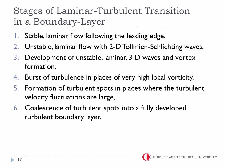
Stages of Laminar-Turbulent Transition
in a Boundary-Layer
1. Stable, laminar flow following the leading edge,
2. Unstable, laminar flow with 2-D Tollmien-Schlichting waves,
3. Development of unstable, laminar, 3-D waves and vortex
formation,
4. Burst of turbulence in places of very high local vorticity,
5. Formation of turbulent spots in places where the turbulent
velocity fluctuations are large,
6. Coalescence of turbulent spots into a fully developed
turbulent boundary layer.
17

Stages of Laminar-Turbulent Transition
in a Boundary-Layer
18
Stages of Laminar-Turbulent Transition
in a Boundary-Layer
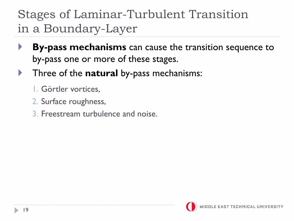
By-pass mechanisms can cause the transition sequence to
by-pass one or more of these stages.
Three of the natural by-pass mechanisms:
1. Görtler vortices,
2. Surface roughness,
3. Freestream turbulence and noise.
19
Stages of Laminar-Turbulent Transition
in a Boundary-Layer
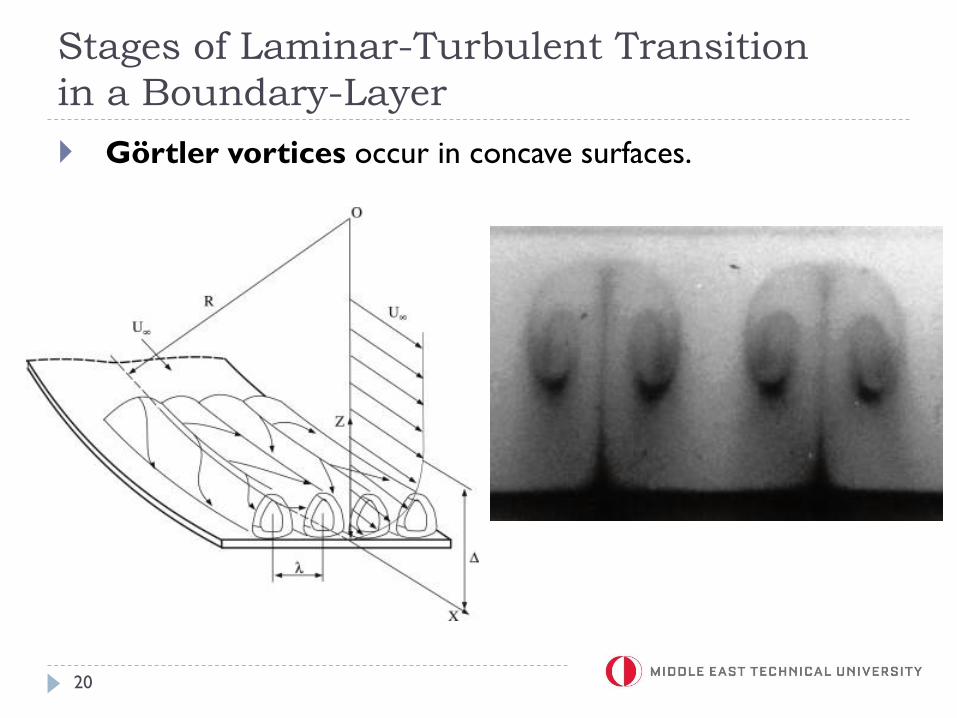
Görtler vortices occur in concave surfaces.
20

Stages of Laminar-Turbulent Transition
in a Boundary-Layer
The centrigugal force acts in the direction of smaller velocity.
This is like heavier fluid flowing over a lighter fluid (like a
water-oil flow).
As a result, the particles subject to greater centrifugal forces
will penetrate into the particles subject to smaller centrifugal
forces.
As a result, peak and valley structures called Görtler vortices
will occur even before 2-D Tollmien-Schlichting waves and
3-D instabilities will be observed.
21
Stages of Laminar-Turbulent Transition
in a Boundary-Layer
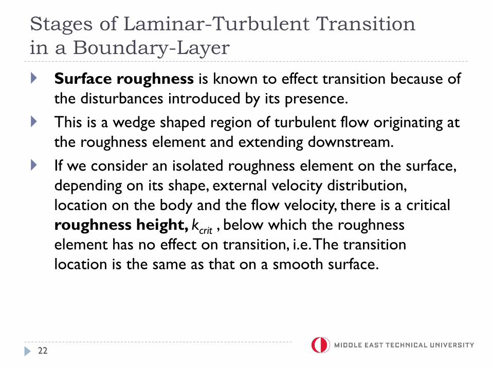
Surface roughness is known to effect transition because of
the disturbances introduced by its presence.
This is a wedge shaped region of turbulent flow originating at
the roughness element and extending downstream.
If we consider an isolated roughness element on the surface,
depending on its shape, external velocity distribution,
location on the body and the flow velocity, there is a critical
roughness height, kcrit , below which the roughness
element has no effect on transition, i.e. The transition
location is the same as that on a smooth surface.
22

Stages of Laminar-Turbulent Transition
in a Boundary-Layer
23

Stages of Laminar-Turbulent Transition
in a Boundary-Layer
As the height of the roughness element increases, a second
critical value, k*crit is reached for which the transition occurs
at the immediate downstream of the roughness element.
This is a wedge shaped region of turbulent flow trailing
downstream with the roughness element at its apex and with
a semi-angle ≈10o.
24

Stages of Laminar-Turbulent Transition
in a Boundary-Layer
Intensity of freestream turbulence:
Transition Reynolds number increases with decreasing
freestream turbulence intensity until a maximum is reached.
Further reductions in turbulence intensity do not improve or
delay transition.
Corrections to smooth transition data, e.g. to the en data.
n = -8.43 - 2.4Tu
25
∞
2
u U
u′=T

Stages of Laminar-Turbulent Transition
in a Boundary-Layer
In addition to natural by-pass mechanisms, there are artificial
by-pass mechanisms which are used as research tools or
means of control:
Vibrating ribbon (maybe spanwise periodic as well),
Pneumatic turbulators.
26
Receptivity
Amplitude and spectral (frequency) characteristics of the
disturbances inside the laminar boundary-layer strongly
influence which type of transition occurs and the major need
in this area is to understand how freestream disturbances are
entrained into the boundary-layer, namely the receptivity
problem.
Receptivity: mechanisms that cause freestream
disturbances to enter the boundary-layer and create initial
amplitudes for unstable waves.
27
Receptivity
If initial amplitudes of disturbances are small, linear
modes of the boundary-layer will be excited, which will
result in the Tollmien-Schlichting waves.
If initial amplitudes are large non-linear modes will be excited
and premature transition will occur through the by-pass
mechanisms.
Mathematically, the receptivity problem is also different from
the stability problem.
28
Receptivity
Receptivity has many different paths to introduce a
disturbance into the boundary layer. These include:
Interaction of freestream turbulence and acoustical
disturbances,
Leading edge curvature,
Discontinuities on the surface contour or inhomogenuities.
29
Receptivity
Stability problem deals with normal mode disturbances
within the boundary-layer. These are determined from the
solution of linearized Navier-Stokes equations and are
ordinary differential equations and the problem becomes an
eigenvalue problem.
On the other hand, in the receptivity problem, neither the
equations nor the boundary conditions are homogeneous.
Boundary-layer is forced externally by a disturbance. Thus,
the receptivity problem is an initial value problem and
requires the solution of full Navier-Stokes equations.
30
Elements of Stability Theory
The stability theory is concerned with individual sine
waves propagating in the boundary-layer, parallel to the
wall.
Amplitudes of the waves vary through the boundary-layer
and are small enough so that linear theory may be used.
Frequency of a wave is and the wave numbers is
k = 2, where is the wavelength.
Two-dimensional waves: lines of constant phase normal to
the freestream direction.
Oblique waves: wavenumber is a vector.
31

Elements of Stability Theory
Phase velocity, c < freestream velocity U
At some point in the boundary-layer, the mean flow velocity
is = c (critical layer).
Wave amplitude usually has a maximum near the critical
layer.
Numerical results calculated from stability theory are usually
presented in a Re- space.
Recr: the Reynolds number below which no amplification is
possible. It only tells where the instability starts. Recr ≠Retr .
32

Elements of Stability Theory
A wave which is introduced into a steady boundary-layer
with a particular frequency will preserve its frequency as it
propagates downstream, while the wavenumber will change.
33
Elements of Stability Theory
A wave which is introduced into a steady boundary-layer
with a particular frequency will preserve its frequency as it
propagates downstream, while the wavenumber will change.
0 Reo: damping,
Reo Re1 : amplification,
Re1 : damping.
If the amplitude of a wave becomes large enough before Re1
is reached, then the nonlinear processes which eventually
lead to transition will take over, and the wave will continue to
grow even though the linear theory says it should damp.
34
Elements of Stability Theory
The linear stability theory can be used to find:
Amplification and damping rates,
Frequency, wavenumber and Reynolds number of waves,
Amplification rates as a function of frequency at a given Re,
Amplitude history of a constant frequency wave as it travels through
the unstable region.
This can be calculated as a ratio of the amplitude to some (generally
unknown) initial amplitude once the amplification rates are known.
Given some initial disturbance spectrum, it is possible to identify the
frequency whose amplitude has increased the most at each Reynolds
number. It is probably one of these frequencies that triggers the
whole transition process after reaching a critical amplitude.
35


