
Aggregate Planning
Operations Management
Dr. Ron Tibben-Lembke

Learning ObjectivesLearning Objectives
Describe planning Distinguish the types of plans Define aggregate scheduling Relate aggregate scheduling to the overall
planning process Explain aggregate scheduling options Develop aggregate schedules
ExampleExample
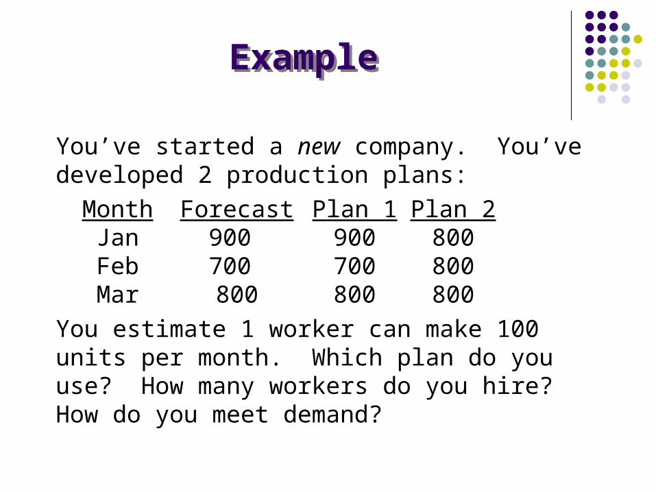
You’ve started a new company. You’ve developed 2 production plans:
Month Forecast Plan 1 Plan 2Jan 900 900 800Feb 700 700 800Mar 800 800 800
You estimate 1 worker can make 100 units per month. Which plan do you use? How many workers do you hire? How do you meet demand?

PlanningPlanning
Setting goals & objectives Example: Meet demand within the limits
of available resources at the least cost Determining steps to achieve goals
Example: Hire more workers Setting start & completion dates
Example: Begin hiring in Jan.; finish, Mar. Assigning responsibility
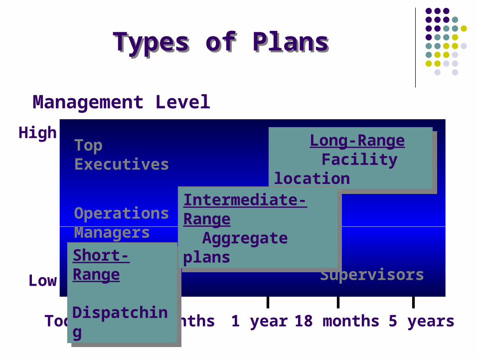
Types of PlansTypes of Plans
Today 3 months 1 year 5 years
Long-Range Facility location
Long-Range Facility location
Short-Range Dispatching
Short-Range Dispatching
Management Level
High
Low
Top Executives
Supervisors
Operations Managers
18 months
Intermediate-Range Aggregate plans
Intermediate-Range Aggregate plans
Aggregate Scheduling Aggregate Scheduling
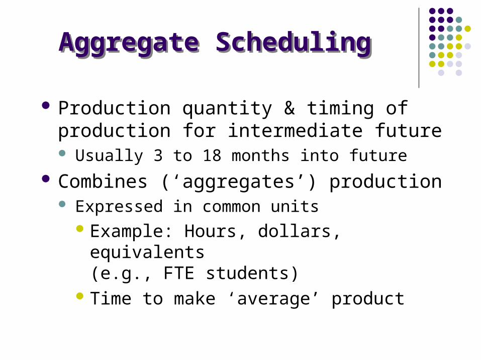
Production quantity & timing of production for intermediate future Usually 3 to 18 months into future
Combines (‘aggregates’) production Expressed in common units
Example: Hours, dollars, equivalents (e.g., FTE students)
Time to make ‘average’ product
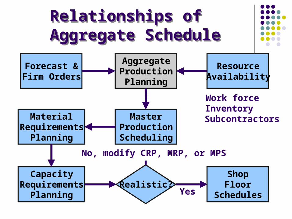
Relationships of Aggregate ScheduleRelationships of Aggregate Schedule
Forecast &Firm Orders
MaterialRequirements
Planning
AggregateProductionPlanning
ResourceAvailability
MasterProductionScheduling
ShopFloor
Schedules
CapacityRequirements
PlanningRealistic?
Yes
No, modify CRP, MRP, or MPS
Work forceInventorySubcontractors
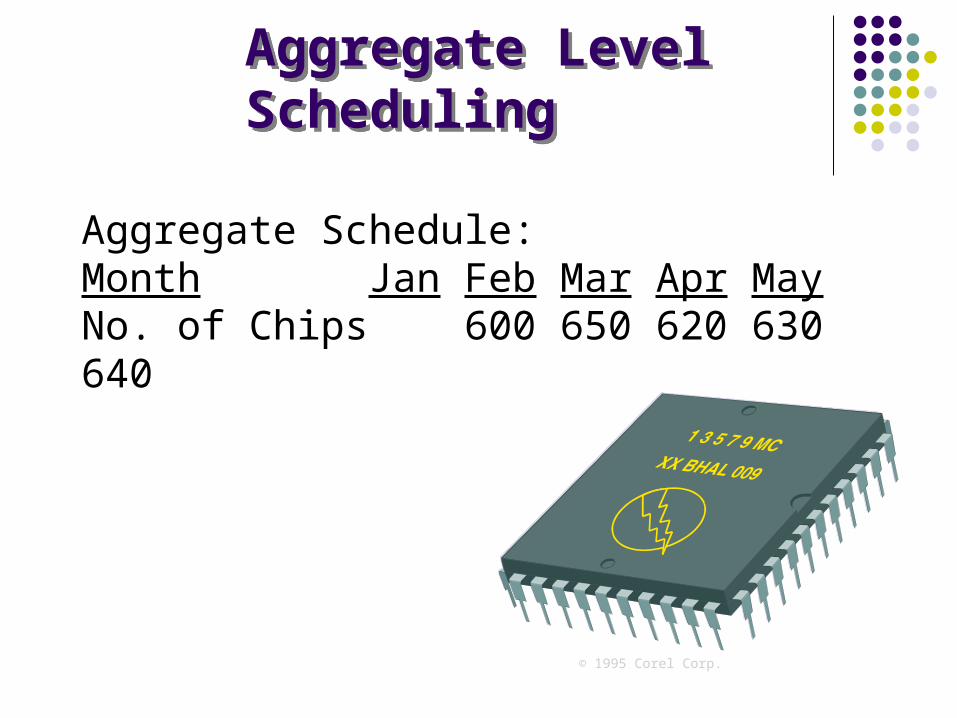
Aggregate Level SchedulingAggregate Level Scheduling
Aggregate Schedule:Month Jan Feb Mar Apr MayNo. of Chips 600 650 620 630 640
© 1995 Corel Corp.
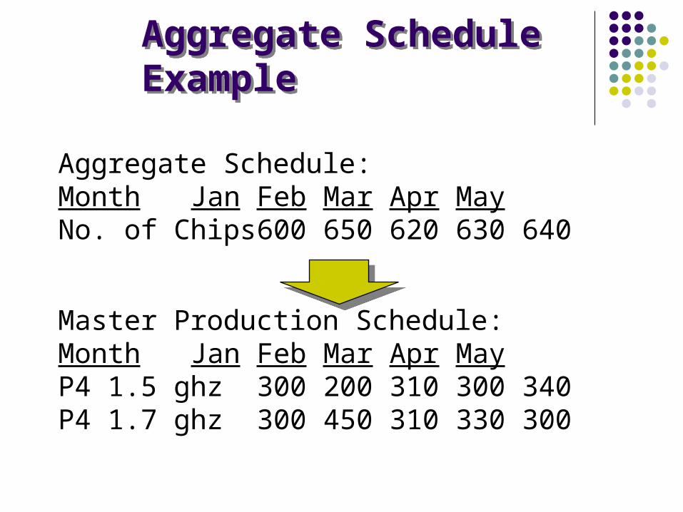
Aggregate Schedule ExampleAggregate Schedule Example
Aggregate Schedule:Month Jan Feb Mar Apr MayNo. of Chips 600 650 620 630 640
Master Production Schedule:Month Jan Feb Mar Apr MayP4 1.5 ghz 300 200 310 300 340P4 1.7 ghz 300 450 310 330 300
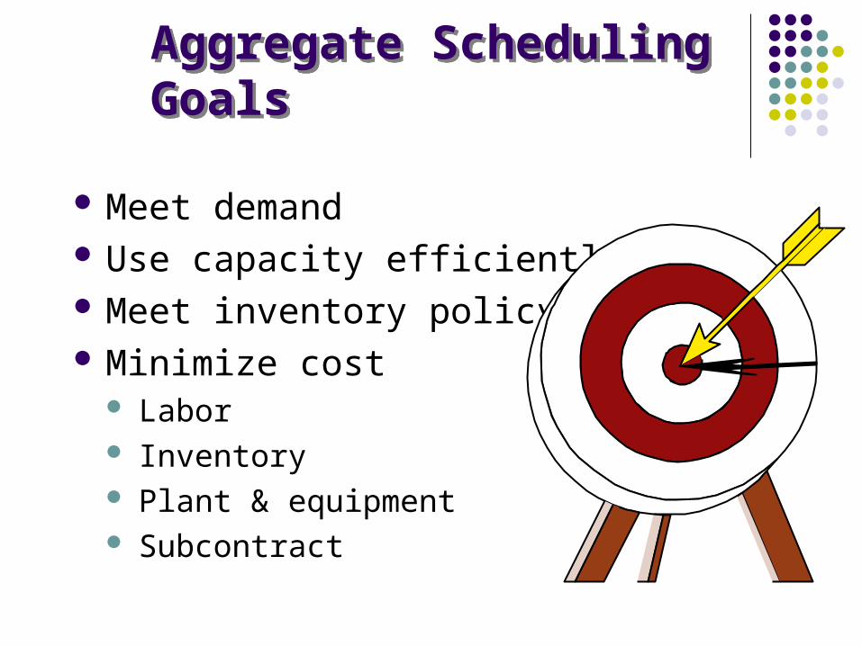
Aggregate Scheduling GoalsAggregate Scheduling Goals
Meet demand Use capacity efficiently Meet inventory policy Minimize cost
Labor Inventory Plant & equipment Subcontract
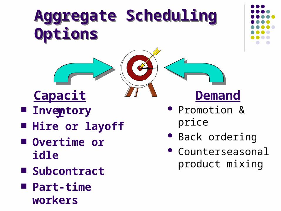
Promotion & price Back ordering Counterseasonal
product mixing
Aggregate Scheduling OptionsAggregate Scheduling Options
Capacity
Demand Inventory Hire or layoff Overtime or idle Subcontract Part-time workers Outsource
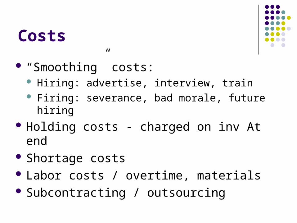
Costs
“Smoothing” costs: Hiring: advertise, interview, train Firing: severance, bad morale, future hiring
Holding costs - charged on inv At end Shortage costs Labor costs / overtime, materials Subcontracting / outsourcing
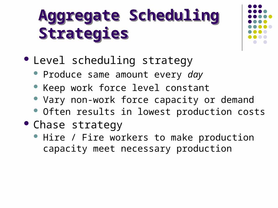
Aggregate Scheduling StrategiesAggregate Scheduling Strategies
Level scheduling strategy Produce same amount every day Keep work force level constant Vary non-work force capacity or demand Often results in lowest production costs
Chase strategy Hire / Fire workers to make production capacity
meet necessary production
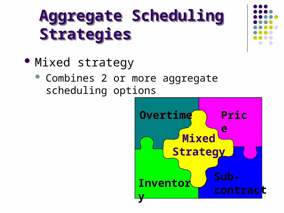
Aggregate Scheduling StrategiesAggregate Scheduling Strategies
Mixed strategy Combines 2 or more aggregate scheduling
options
Overtime
Sub-contract
Inventory
Price
Mixed Strategy
Aggregate Scheduling MethodsAggregate Scheduling Methods
Graphical & charting techniques Popular & easy-to-understand Trial & error approach
Mathematical approaches Linear Programming Simulation More involved, but usually better answers
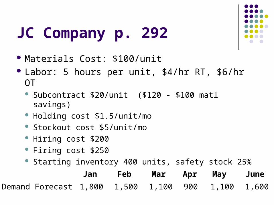
JC Company p. 292
Materials Cost: $100/unit Labor: 5 hours per unit, $4/hr RT, $6/hr OT
Subcontract $20/unit ($120 - $100 matl savings) Holding cost $1.5/unit/mo Stockout cost $5/unit/mo Hiring cost $200 Firing cost $250 Starting inventory 400 units, safety stock 25%
Jan Feb Mar Apr May June
Demand Forecast 1,800 1,500 1,100 900 1,100 1,600
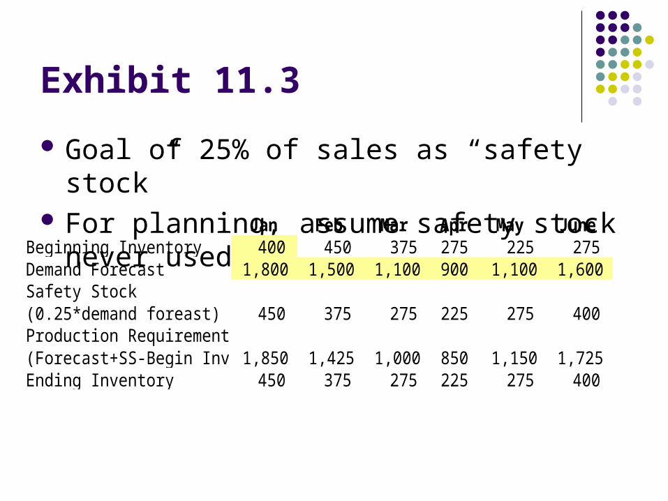
Exhibit 11.3
Goal of 25% of sales as “safety stock” For planning, assume safety stock never used
Jan Feb Mar Apr May JuneBeginning Inventory 400 450 375 275 225 275 Demand Forecast 1,800 1,500 1,100 900 1,100 1,600 Safety Stock (0.25*demand foreast) 450 375 275 225 275 400 Production Requirement (Forecast+SS-Begin Inv) 1,850 1,425 1,000 850 1,150 1,725 Ending Inventory 450 375 275 225 275 400
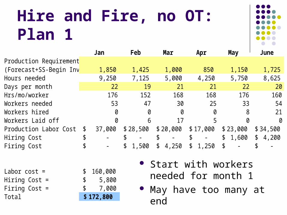
Hire and Fire, no OT: Plan 1Jan Feb Mar Apr May June
Production Requirement (Forecast+SS-Begin Inv) 1,850 1,425 1,000 850 1,150 1,725 Hours needed 9,250 7,125 5,000 4,250 5,750 8,625 Days per month 22 19 21 21 22 20Hrs/mo/worker 176 152 168 168 176 160Workers needed 53 47 30 25 33 54Workers hired 0 0 0 0 8 21Workers Laid off 0 6 17 5 0 0Production Labor Cost 37,000$ 28,500$ 20,000$ 17,000$ 23,000$ 34,500$ Hiring Cost -$ -$ -$ -$ 1,600$ 4,200$ Firing Cost -$ 1,500$ 4,250$ 1,250$ -$ -$
Labor cost = 160,000$ Hiring Cost = 5,800$ Firing Cost = 7,000$ Total 172,800$
Start with workers needed for month 1
May have too many at end
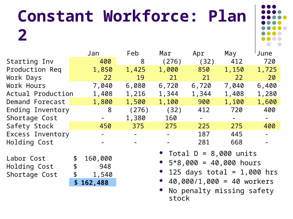
Constant Workforce: Plan 2Jan Feb Mar Apr May June
Starting Inv 400 8 (276) (32) 412 720 Production Req 1,850 1,425 1,000 850 1,150 1,725 Work Days 22 19 21 21 22 20 Work Hours 7,040 6,080 6,720 6,720 7,040 6,400 Actual Production 1,408 1,216 1,344 1,344 1,408 1,280 Demand Forecast 1,800 1,500 1,100 900 1,100 1,600 Ending Inventory 8 (276) (32) 412 720 400 Shortage Cost - 1,380 160 - - - Safety Stock 450 375 275 225 275 400 Excess Inventory - - - 187 445 - Holding Cost - - - 281 668 -
Labor Cost 160,000$ Holding Cost 948$ Shortage Cost 1,540$
162,488$
Total D = 8,000 units 5*8,000 = 40,000 hours 125 days total = 1,000 hrs 40,000/1,000 = 40 workers No penalty missing safety stock
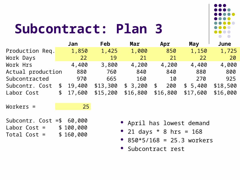
Subcontract: Plan 3Jan Feb Mar Apr May June
Production Req. 1,850 1,425 1,000 850 1,150 1,725 Work Days 22 19 21 21 22 20 Work Hrs 4,400 3,800 4,200 4,200 4,400 4,000 Actual production 880 760 840 840 880 800 Subcontracted 970 665 160 10 270 925 Subcontr. Cost 19,400$ 13,300$ 3,200$ 200$ 5,400$ 18,500$ Labor Cost 17,600$ 15,200$ 16,800$ 16,800$ 17,600$ 16,000$
Workers = 25
Subcontr. Cost = 60,000$ Labor Cost = 100,000$ Total Cost = 160,000$
April has lowest demand 21 days * 8 hrs = 168 850*5/168 = 25.3 workers Subcontract rest
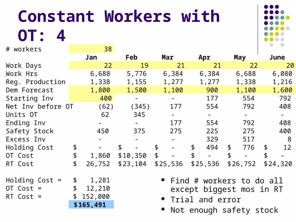
# workers 38Jan Feb Mar Apr May June
Work Days 22 19 21 21 22 20Work Hrs 6,688 5,776 6,384 6,384 6,688 6,080 Reg. Production 1,338 1,155 1,277 1,277 1,338 1,216 Dem Forecast 1,800 1,500 1,100 900 1,100 1,600 Starting Inv 400 - - 177 554 792 Net Inv before OT (62) (345) 177 554 792 408 Units OT 62 345 - - - - Ending Inv - - 177 554 792 408 Safety Stock 450 375 275 225 275 400 Excess Inv - - - 329 517 8 Holding Cost -$ -$ -$ 494$ 776$ 12$ OT Cost 1,860$ 10,350$ -$ -$ -$ -$ RT Cost 26,752$ 23,104$ 25,536$ 25,536$ 26,752$ 24,320$
Holding Cost = 1,281$ OT Cost = 12,210$ RT Cost = 152,000$
165,491$
Constant Workers with OT: 4
Find # workers to do all except biggest mos in RT
Trial and error Not enough safety stock
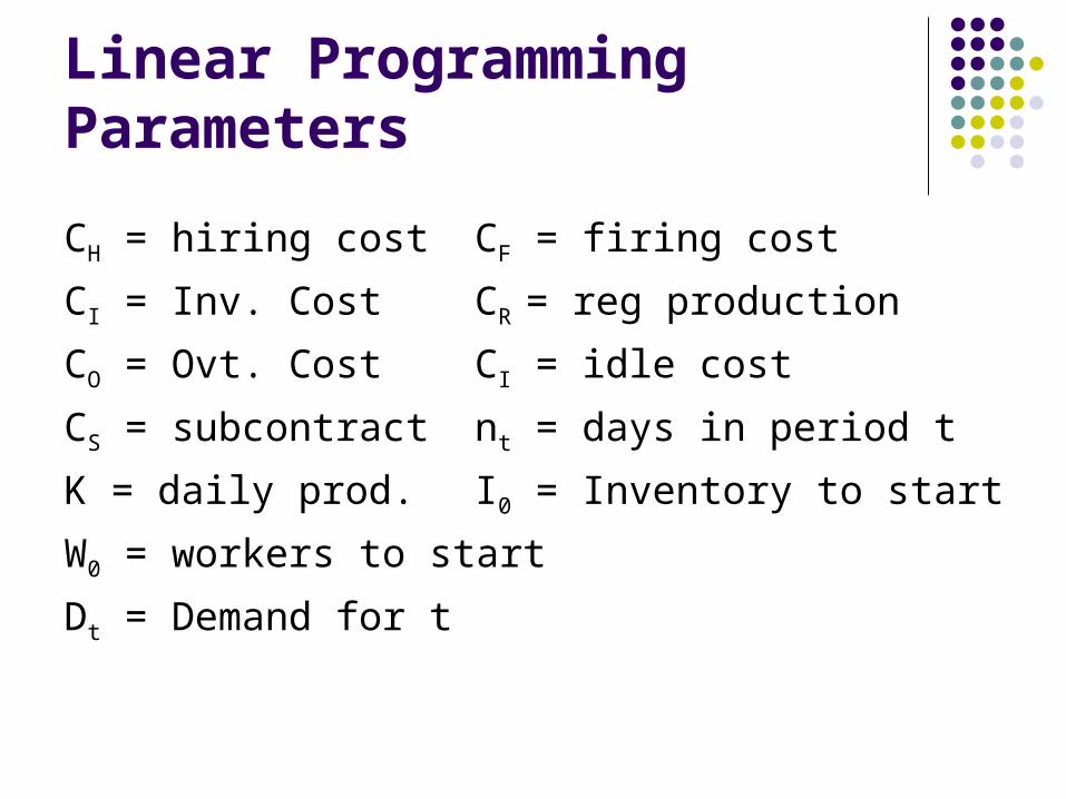
Linear Programming Parameters
CH = hiring cost CF = firing cost
CI = Inv. Cost CR = reg production
CO = Ovt. Cost CI = idle cost
CS = subcontract nt = days in period t
K = daily prod. I0 = Inventory to start
W0 = workers to start
Dt = Demand for t
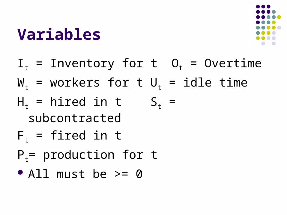
Variables
It = Inventory for t Ot = Overtime
Wt = workers for t Ut = idle time
Ht = hired in t St = subcontracted
Ft = fired in t
Pt= production for t All must be >= 0
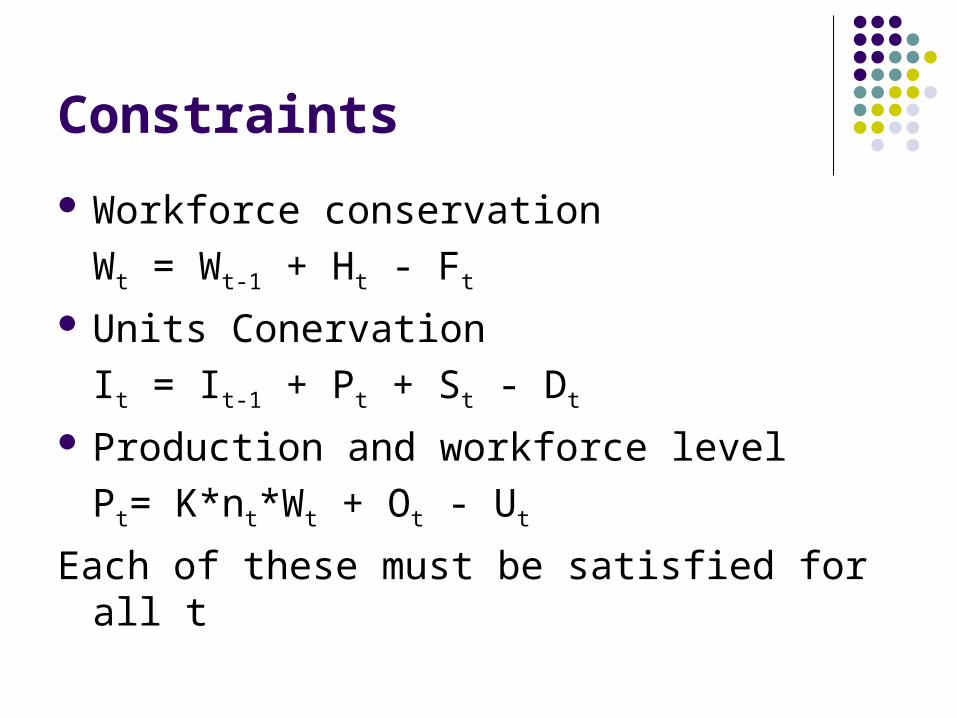
Constraints
Workforce conservation
Wt = Wt-1 + Ht - Ft
Units Conervation
It = It-1 + Pt + St - Dt
Production and workforce level
Pt= K*nt*Wt + Ot - Ut
Each of these must be satisfied for all t
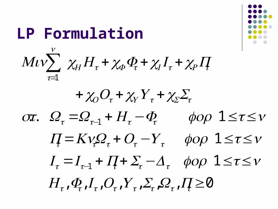
LP Formulation
0,,,,,,,
1
1
1..
1
1
1
≥≤≤−++=≤≤−+=≤≤−+=
+++
+++
−
−
=∑
tttttttt
ttttt
ttttt
tttt
tStUtO
tRtItFtH
n
t
PWSUOIFHntforDSPIIntforUOWKnPntforFHWWts
ScUcOc
PcIcFcHcMin
LP Considerations
LP can be modified to include minimum inv. level each period
Negative inventory can be allowed Care needed when rounding
ConclusionConclusion
Described role of aggregate planning Described types of plans Explained aggregate scheduling options Developed aggregate schedules
Chase, Level, and Hybrid Linear Programming


