

Abstract—Batch dryers are some of the most widespread
equipment used for fruit dehydration. Nevertheless, the optimization
of the air distribution inside the drying chamber of a batch dryer
remains a very important point, due to its strong effect on drying
efficiency as well as the uniformity of the moisture content of the
drying products. A new scale laboratory batch-type tray air (BTA)
dryer was designed, constructed and evaluated for the drying of
several horticultural and agricultural products. The airflow field
inside the dryer was studied through a commercial computational
fluid dynamics (CFD) package. A three-dimensional model for a
laboratory BTA dryer was created and the steady-state
incompressible, Reynolds-Averaged Navier-Stokes equations that
formulate the flow problem were solved, incorporating standard and
RNG k-ε turbulence models. In the simulation, the tray, used inside
the BTA drying chamber, was modeled as a thin porous media of
finite thickness. The simulations for testing the chamber were
conducted at an average velocity of 2.9 m/s at ambient temperature.
The CFD models were evaluated by comparing the airflow patterns
and velocity distributions to the measured data. Numerical
simulations and measurements showed that the new scale laboratory
BTA dryer is able to produce a sufficiently uniform air distribution
throughout the testing chamber of the dryer.
Keywords— Airflow, Batch dryer, CFD, Simulation.
I. INTRODUCTION
NE the most important factors in the designing of
conventional batch-type air dryers is the airflow design.
In industrial air dryers the effect of flow heterogeneity is
particularly difficult to resolve. The distribution of airflow
D. A. Tzempelikos is PhD Student in the Fluid Mechanics Laboratory,
Department of Mechanical Engineering and Aeronautics, University of
Patras, GR-26500 Patras, GREECE (corresponding author, phone: +30-210-
2896838; fax: +30-210-2896838; e-mail: [email protected]).
A. P. Vouros is PhD Researcher in the Laboratory of Fluid Mechanics and
Turbomachinery, Department of Mechanical Engineering Educators, School
of Pedagogical and Technological Education (ASPETE), GR-14121 Athens,
GREECE (e-mail: [email protected]).
A. V. Bardakas is undergraduate student in the Laboratory of Fluid
Mechanics and Turbomachinery, Department of Mechanical Engineering
Educators, School of Pedagogical and Technological Education (ASPETE),
GR-14121 Athens, GREECE (e-mail: [email protected]).
A. E. Filios is Professor in the Laboratory of Fluid Mechanics and
Turbomachinery, Department of Mechanical Engineering Educators, School
of Pedagogical and Technological Education (ASPETE), GR-14121 Athens,
GREECE (e-mail: [email protected]).
D. P. Margaris is Associate Professor in the Fluid Mechanics Laboratory,
Department of Mechanical Engineering and Aeronautics, University of
Patras, GR-26500 Patras, GREECE (e-mail: margaris @mech.upatras.gr).
depends on the process of drying, the drying medium and the
geometry of the drying chamber. These factors determine the
uniformity of drying and thus the quality of the finished
products. Even though the performance of a drying chamber
can be studied experimentally, such a research restricts the
generalization of the results and certainly cannot be applied to
the original design of the drying chamber due to time and cost
limitations. In contrast, with the help of computational fluid
dynamics (CFD), which can span a wide range of industrial
and non-industrial applications, the complexity of the flow
field can be solved numerically.
Mathioulakis, Karathanos and Belessiotis [1] simulated the
air flow in an industrial batch-type tray air dryer. The
distribution of pressure and velocity over the product were
found to lack in spatial homogeneity which led to variations in
drying rates and moisture contents.
Margaris and Ghiaus [2] simulated the airflow in an
industrial drier and provided parameters for different
configurations that helped to optimize the drying space with
significant improvement to the quality of the dried product and
the reduction of energy consumption. Mirade [3] used a two-
dimensional CFD model with time dependent boundary
conditions, studying the distribution uniformity of air velocity
in an industrial meat dryer for the low and high levels of a
ventilation cycle. Hoang, Verbonen, Baerdemaeker and
Nicolai [4] simulated the airflow inside a cold store solving the
steady state incompressible, Reynolds-averaged Navier-Stokes
(RANS) equations by applying the standard k-ε and the RNG
k-ε turbulence models. The results showed that the RNG k-ε
model does not improve the prediction of air recirculation
whereas any improvements would require a finer grid with an
enhanced simulation of a turbulent flow. Amanlou and
Zomordian [5] designed a new fruit cabinet with various
geometries and then simulated these geometries using CFD.
The experimental results and the predicted data from the CFD
revealed a very good correlation coefficient for the drying air
temperature and the air velocity in the drying chamber. Norton
and Sun [6] in a review paper demonstrated the widely use of
CFD for predicting air velocity and temperature in drying
chambers while Scott and Richardson [7] and Xia and Sun [8]
presented the commercial CFD software that are being
increasingly employed in the food industry.
Recent studies have shown that only a limited research on
Analysis of air velocity distribution in a
laboratory batch-type tray air dryer by
computational fluid dynamics
D. A. Tzempelikos, A. P. Vouros, A. V. Bardakas, A. E. Filios, and D. P. Margaris
O
INTERNATIONAL JOURNAL OF MATHEMATICS AND COMPUTERS IN SIMULATION
Issue 5, Volume 6, 2012 413

the prediction and measurements of flow and pressure fields in
BTA dryers has been performed. The absence of experiments
can be attributed to the difficulty of direct measurements of the
local air velocity and flow into a drying chamber for
horticultural and agricultural products.
The present study concerns the design, construction and
evaluation of a new scale laboratory BTA dryer which can host
thermal drying studies in fully controllable environment. The
velocity and pressure fields are analyzed with the aid of the
commercial CFD code Fluent®. For the numerical simulations,
the steady state RANS equations are solved in combination
with the standard k-ε and the RNG k-ε turbulence models. The
effect of the k-ε and the RNG k-ε turbulence models is
distinguished through direct comparisons of the derived
airflow patterns. The purposes of the current research are: a)
the study of the velocity fields in the drying chamber of a new
scale laboratory BTA dryer while building a CFD method that
is affordable in terms of computation time, and b) the
comparison between the numerical results and the
experimental measurements gathered with a velocity sensor.
II. EXPERIMENTAL SETUP AND MEASUREMENTS
A. Description of the BTA dryer
The lab scale BTA dryer which has been designed and
constructed in the Laboratory of Fluid Mechanics and
Turbomachinery in ASPETE, is shown in Fig. 1 and 2. The
overall dimensions of the facility are 4.7 m (length), 2.5 m
(width) and 2.5 m (height). The air ducts are made from steel
of 0.8 mm thickness. All the ducts are insulated with 10 mm
Alveolen (Frelen) which has a thermal conductivity of 0.032
W/m.K and water absorption of 0.011 kg/m
2.
Fig. 1 Schematic diagram of the lab-scale BTA dryer
The square section drying chamber (0.5m x 0.5m) is of
tower (vertical) type and is equipped with a metal tray which is
supported on four, side wall-mounted, load cells. A set of four
refractory glasses of 10 mm thickness are available to replace
the side steel walls when optical clarity and precise visual
observations are required.
Upstream of the drying chamber, the following parts are
located: a long rectangular diffuser with a total divergence
angle of 6.7 deg, a tube heat exchanger in which the hot water
is provided through a boiler of 58 kW (50,000 kcal/h) thermal
power, a transitional duct with observation window that
includes a sprayer for humidifying purposes, a corner duct that
incorporates four guide vanes and finally a flow straightener
section. The flow straighteners, consisting of an aluminum
honeycomb (made from 3003 aluminum alloy foil) with a cell
size of 1/4' and 38 mm thickness and screen wires located
downstream of the honeycomb, are considered necessary for
flow uniformity in the drying section. The flow rate is
observed and controlled with a custom made and calibrated
rake of pitot tubes (namely pitot rake) located at the inlet of
the drying chamber.
Downstream of the vertical drying chamber, the following
parts are located: a second corner duct with guide vanes, an
elevated horizontal modular constructed duct, an outlet
dumper and an exit diffuser. The modular design of the facility
permits the easy placement of two or three horizontal drying
chambers in tandem arrangement, on the elevated return or exit
flow leg.
The air flow is established and controlled through a
centrifugal fan directly driven by a 3 phase electric motor of 3
kW with its speed regulated by an AC inverter. Adjusting the
air dampers, the laboratory BTA dryer can be used for thermal
drying experimental studies in both open circuit and close
circuit operations.
Fig. 2 Photo of the lab-scale BTA dryer, equipped with measuring
instrumentation and data acquisition system
B. Measurements
The air velocity experiments inside the drying chamber,
under ambient conditions, i.e. atmospheric pressure at 18.4 oC,
were carried out with a constant speed of the induced
centrifugal fan of 690 rpm at 23 Hz. The volumetric flow rate
was 2,600 m3/h, resulting to a mean velocity of 2.9 m/s and a
Reynolds number of 9.9 x10⁴ (based on the hydraulic diameter
of the drying chamber).
The mean speed of the air flow at the inlet was the weighted
average velocity of the 12 points collected from the pitot rake
arrangement, as shown in Fig. 3, and the four pressure taps
(same level with the contact tip of the pitot tube) on the side
wall of the inlet of the drying chamber.
Each pitot tube is connected via plastic tubing to a custom
INTERNATIONAL JOURNAL OF MATHEMATICS AND COMPUTERS IN SIMULATION
Issue 5, Volume 6, 2012 414

made pressure collector system equipped with solenoid valves
(Tekmatic 24VDC, 6W) which allows its operation and
control using a custom-made software developed in Labview®.
A differential pressure transmitter (Dwyer, model MS-121-
LCD) with a calibrated accuracy (± 2%) in the range of 25 Pa
was used to measure each of the 12 points with an automatic
“open-close” function of the proper solenoid valve.
Fig. 3 The pitot tubes rake
For cross checking purposes of the pitot-static measured
velocities, a velocity reference transducer (54T29, Dantec
Dynamics® with 54N81 Multichannel CTA) was used, which
offers the best value for cost and accuracy. The velocity range
of the sensor is 0 – 30 m/s. The calibrated accuracy is ± 2% of
reading ± 0.02 m/s or 2.6 % of the selected range of 3 m/s,
which is assured by a certificate provided by the manufacturer.
The measurement of the velocity was done inside the duct at
a distance of 0.51 m from the inlet of the drying chamber. In
order to measure the air velocity during each test and at
different locations of the drying chamber, 4 holes on the side
wall of the drying chamber were pierced (Fig. 2 and 4). All
holes, except the one through which the velocity transducer
was inserted for the air velocity measurement, were filled
tightly with conic plastic washers. The inlet air velocity was
kept constant during the experiment.
In order to read the velocity at each point inside the drying
cabinet, the velocity transducer was inserted through a side
wall proximity hole and adjusted at eight different locations
along the depth of the drying chamber. At each point the time
averaged velocity was determined from the measurements
which had a frequency of 200 Hz and averaged over a 10
second period. The experimental values were directly
compared with the numerical predictions at the same locations.
Both the differential pressure transmitter and the velocity
transducer were connected to a PC with the NI (National
Instruments®) PCIe-6321 DAQ device via the NI SCXI-1000
and NI SCXI-1302 modules. Custom made software in
Labview® was used to interface with the data acquisition.
Fig. 4 A 3d view section of the drying chamber with the location of
the measured velocities (dimensions in millimeters)
The overall accuracy of the CFD calculations is calculated
as the average of the absolute differences between the time-
averaged velocity magnitude for the CFD calculation and the
measurement at each position, divided by the average velocity
magnitude in the drying chamber obtained from the
measurements and is expressed as:
1
1
100
mj j
cfd exp
j
mj
exp
j
U U
E
U
=
=
−
= ×∑
∑
(1)
where j
cfdU is the velocity at a position j for the CFD
calculations, j
expU is the average velocity at a position j for the
measurement and m is the number of measurement points.
III. NUMERICAL SIMULATION
The numerical computation of fluid transport employs the
conservation of mass, momentum and turbulence model
equations. The Gambit® preprocessor was used to create
geometry, to discretize the fluid domain into small cells that
could form a volume mesh and to set up the appropriate
boundary conditions. The flow properties could then be
specified, the equations were solved and the results were
analyzed using Fluent®.
A. Governing equations
The governing equations based on the conservation of mass
and momentum of a Newtonian fluid flow, which apply to an
infinitesimal small volume in a Cartesian co-ordinate system
(x, y, z) using the Reynolds averaged formulation [9], are:
0divUt
ρ∂+ =
∂
(2)
( ) ( ) ( )i
i eff i i
i
u pdiv Uu div gradu S
t x
ρρ µ
∂ ∂+ = − +
∂ ∂
(3)
( )p,Tρ ρ=
(4)
eff Tµ µ µ= +
(5)
INTERNATIONAL JOURNAL OF MATHEMATICS AND COMPUTERS IN SIMULATION
Issue 5, Volume 6, 2012 415

In these formulae, U is the velocity vector, consisting of
three components ux, uy, uz (m/s), p is the pressure (Pa) and T
is the temperature (oC). The density ρ (kg/m
3) and the laminar
viscosity µ (N.s/m
2) are the only fluid properties involved; µΤ
and µeff are the turbulent and effective viscosity, respectively.
The Si sources contain further contributions from the viscous
stress term and may contain additional body forces. In all
current calculations, constant air properties has been
considered (ρ = 1.225 kg/m3 and µ = 1.7894 x 10
-5 N
.s/m
2).
B. Turbulence models
The k-ε turbulence models are the most widely used and
validated turbulence models in literature. The k-ε turbulence
models use an eddy-viscosity assumption for the turbulence,
expressing the turbulent stresses as an additional viscous stress
term in (5). In the k-ε turbulence model, the turbulent viscosity
is expressed in terms of two variables: the turbulence kinetic
energy (TKE) k and the rate of dissipation of turbulent energy
ε.
B.1 Standard k-ε turbulence model
The standard k-ε model which is valid only for fully
turbulent flows, is a semi-empirical model based on model
transport equations for the TKE k and its dissipation rate ε,
containing empirical constants in the production and
destruction terms of the ε equation. The model transport
equation for the turbulence kinetic energy is derived from the
exact equation, while the model transport equation for the
dissipation rate is obtained using physical reasoning and bears
little resemblance to its mathematically exact counterpart [10].
The resulting equations are similar to the governing flow
equations [9]: 2
T
kCµµ ρ
ε=
(6)
( ) ( )k
kdiv Uk div grad k P
t
Τµρρ µ ρε
σ
∂+ − + = −
∂
(7)
( ) ( )
2
1 2
div U div gradt
C P Ck k
Τ
ε
ε ε
µρερ ε µ ε
σ
ε ερ
∂+ − + =
∂
−
(8)
where P is a term containing the turbulence production due
to the stresses in the flow. The standard k-ε model contains
five empirical constants (Cµ, C1ε, C2ε, σk and σε) and during
this study these constants remained the same:
Cµ = 0.09, C1ε = 1.44, C2ε = 1.92, σk = 1.0 and σε = 1.3 (9)
Near walls, the equations do not hold and standard
logarithmic wall profiles have to be implemented. An
important variable is y+, a dimensionless distance normal to
the wall. The value of y+ determines in which region of the
boundary layer the first node is situated. The log-law is valid
only for y+ > 30.
B.2 RNG k-ε turbulence model
The RNG (renormalization group) k-ε model employs a
differential form of the relation for the effective viscosity,
yielding an accurate description of how the effective turbulent
transport varies with the effective Reynolds number. This
allows accurate extension of the model to near-wall flows and
low-Reynolds-number or transitional flows. Furthermore, a
new term appears in the ε equation, which accounts for
anisotropy in strongly strained turbulent flows. The same
default wall functions as in the standard k-ε model are valid in
this case as well. The ε equation is [9]:
( ) ( )
( )2
1 1 2RNG
div U div gradt
C C P Ck k
Τ
ε
ε ε
µρερ ε µ ε
σ
ε ερ
∂+ − + =
∂
− −
(10)
( )0
1RNG 3
n1
nC
1 nβ
−
=+
(11)
0 5,
sP kn
Τµ ε
=
(12)
where n0 and β are additional model constants, which are
equal to 4.38 and 0.012 respectively while Ps is the shear part
of the production. The standard values of the other constants
are considered suitable for this application:
Cµ = 0.0845, C1ε = 1.42, C2ε = 1.68, σk = 0.7179 and
σε = 0.7179 (13)
The k equation has the same format as in the standard k-ε
turbulence model.
C. Model of the tray
A source term was added to the k-ε and the RNG k-ε
turbulence model equations to estimate the pressure drop
across the tray inside the drying chamber. The tray was
calculated as a screen and in the CFD simulation, the screen
was modeled as a thin porous media of finite thickness over
which the pressure change was defined as a combination of
Darcy's Law and an additional inertial loss term which is given
by [10]:
2
2
1
2n np U C U m
µ∆ ρ ∆
α = − +
(14)
where µ is the laminar fluid viscosity, α is the permeability
of the tray, C2 is the pressure-jump coefficient (pressure loss
coefficient per unit thickness), Un is the velocity normal to the
tray, and ∆m is the thickness of the tray.
D. Model of the BTA dryer
The flow field inside the drying chamber of an empty
laboratory BTA dryer, operated in open circuit mode was
numerically studied. The structure of the modeled dryer is
depicted in Fig. 5. The dryer is 4.7 m in length, 0.5 m in width
and 1.38 m in height. The dimensions of the drying chamber
are 0.5 x 0.5 x 0.66 m.
The BTA dryer is modeled with the tray located in a
distance of 0.29 m from the inlet of the drying chamber. The
tray has a length of 0.48 m, a width of 0.48 m and a thickness
INTERNATIONAL JOURNAL OF MATHEMATICS AND COMPUTERS IN SIMULATION
Issue 5, Volume 6, 2012 416
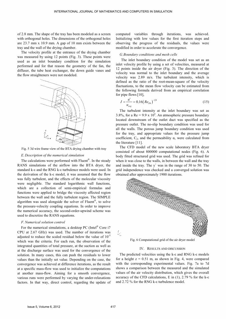
of 2.8 mm. The shape of the tray has been modeled as a screen
with orthogonal holes. The dimensions of the orthogonal holes
are 23.7 mm x 10.9 mm. A gap of 10 mm exists between the
tray and the wall of the drying chamber.
The velocity profile at the entrance of the drying chamber
was measured by using 12 points (Fig. 3). These points were
used as an inlet boundary condition for the simulation
performed and for that reason the geometry of the fan, the
diffuser, the tube heat exchanger, the down guide vanes and
the flow straighteners were not modeled.
Fig. 5 3d wire frame view of the BTA drying chamber with tray
E. Description of the numerical simulation
The calculations were performed with Fluent®. In the steady
RANS simulations of the airflow into the BTA dryer, the
standard k-ε and the RNG k-ε turbulence models were used. In
the derivation of the k-ε model, it was assumed that the flow
was fully turbulent, and the effects of the molecular viscosity
were negligible. The standard logarithmic wall functions,
which are a collection of semi-empirical formulas and
functions were applied to bridge the viscosity affected region
between the wall and the fully turbulent region. The SIMPLE
algorithm was used alongside the solver of Fluent®, to solve
the pressure-velocity coupling equations. In order to improve
the numerical accuracy, the second-order-upwind scheme was
used to discretize the RANS equations.
F. Numerical solution control
For the numerical simulations, a desktop PC (Intel® Core i7
CPU at 2.67 GHz) was used. The number of iterations was
adjusted to reduce the scaled residual below the value of 10-5
which was the criteria. For each run, the observation of the
integrated quantities of total pressure, at the suction as well as
at the discharge surface was used for the convergence of the
solution. In many cases, this can push the residuals to lower
values than the initially set value. Depending on the case, the
convergence was achieved at difference iterations, as the result
at a specific mass-flow was used to initialize the computations
at another mass-flow. Aiming for a smooth convergence,
various runs were performed by varying the under-relaxations
factors. In that way, direct control, regarding the update of
computed variables through iterations, was achieved.
Initializing with low values for the first iteration steps and
observing the progress of the residuals, the values were
modified in order to accelerate the convergence.
G. Boundary conditions and mesh cells
The inlet boundary condition of the model was set as an
inlet velocity profile by using a set of velocities, measured at
12 points inside the air dryer (Fig. 3). The direction of the
velocity was normal to the inlet boundary and the average
velocity was 2.89 m/s. The turbulent intensity, which is
defined as the ratio of the root-mean-square of the velocity
fluctuations, to the mean flow velocity can be estimated from
the following formula derived from an empirical correlation
for pipe flows [10],
( ) 1 80 16 Dh
avg
u, Re
uΙ −′
= =
(15)
The turbulent intensity at the inlet boundary was set as
3.8%, for a Re = 9.9 x 10⁴. An atmospheric pressure boundary
located downstream of the outlet duct was specified as the
pressure outlet. The no-slip boundary condition was used for
all the walls. The porous jump boundary condition was used
for the tray, and appropriate values for the pressure jump
coefficient, C2, and the permeability α, were calculated from
the literature [11].
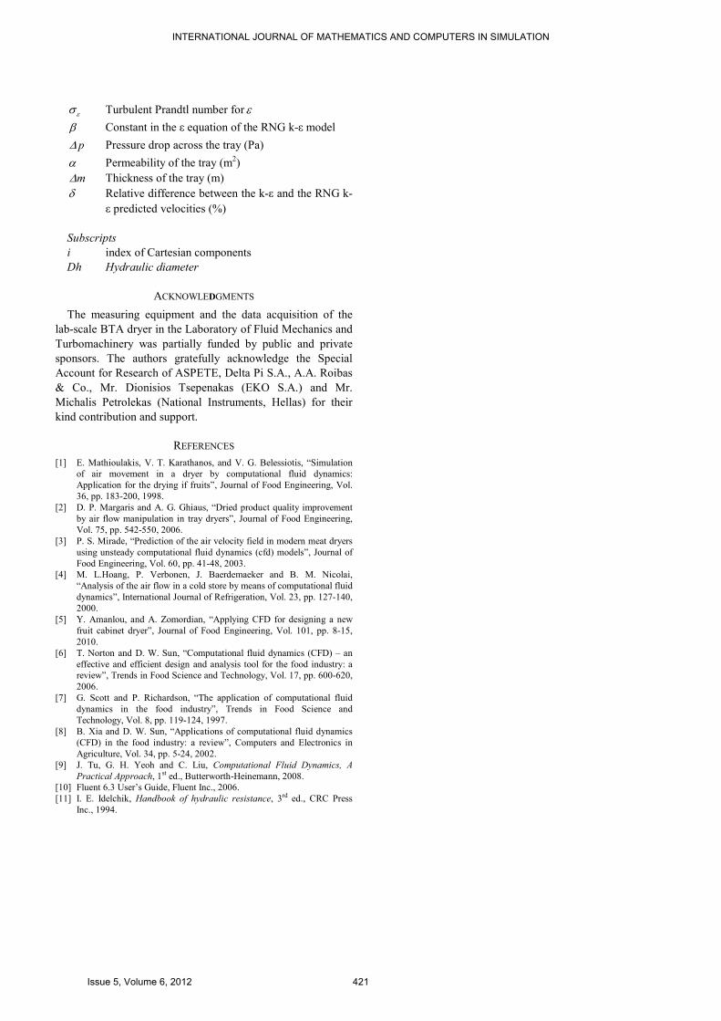
The CFD model of the new scale laboratory BTA dryer
consisted of about 800000 computational nodes (Fig. 6). A
body fitted structured grid was used. The grid was refined for
when it was close to the walls, in between the wall and the tray
and inside the tray. The y+ was in the range of 30 to 50. The
grid independence was checked and a converged solution was
obtained after approximately 1900 iterations.
Fig. 6 Computational grid of the air dryer model
IV. RESULTS AND DISCUSSION
The predicted velocities using the k-ε and RNG k-ε models
for a height z = 0.51 m, as shown in Fig. 4, were compared
with the corresponding experimental values. Fig. 7a to 7d
shows a comparison between the measured and the simulated
values of the air velocity distribution, which gives the overall
accuracy of the CFD calculations, E in (1), 2.79 % for the k-ε
and 2.72 % for the RNG k-ε turbulence model.
INTERNATIONAL JOURNAL OF MATHEMATICS AND COMPUTERS IN SIMULATION
Issue 5, Volume 6, 2012 417

(a) z = 0.51 m, y = 0.163 m
(b) z = 0.51 m, y = 0.223 m
(c) z = 0.51 m, y = 0.283 m
(d) z = 0.51 m, y = 0.343 m
Fig. 7 Velocity field measurements compared with CFD predictions
in the BTA drying chamber
(a) z = 0.51 m, y = 0.163 m)
(b) z = 0.51 m, y = 0.223 m
(c) z = 0.51 m, y = 0.283 m
(d) z = 0.51 m, y = 0.343 m
Fig. 8 Turbulent intensity predictions and comparisons in the BTA
drying chamber
INTERNATIONAL JOURNAL OF MATHEMATICS AND COMPUTERS IN SIMULATION
Issue 5, Volume 6, 2012 418

(a) k-ε turbulence model
(b) RNG k-ε turbulence model
Fig. 9 Velocity contours (m/s) in BTA drying chamber cross section
(z = 0.51 m)
The difference of the absolute between the simulated and
experimental values varied from 0.002 to 0.227 m/s for the k-ε
and from 0.002 to 0.213 m/s for the RNG k-ε turbulence
model.
The relative error between the simulated and experimental
values varied from 0.08 to 7.38 % for the k-ε and from 0.08 to
6.93 % for the RNG k-ε turbulence model.
The average velocity of the experimental values was 3.22
m/s with a standard deviation of 0.12761. The average velocity
and standard deviation for the k-ε and RNG k-ε turbulence
models were 3.274 m/s, 0.09367, 3.267 m/s and 0.10503
respectively.
The overall accuracy of the CFD calculations indicates that
the CFD simulation scheme is practical for the analysis of the
velocity field in the drying chamber.
Fig. 8a to 8d illustrates the turbulent intensity predicted with
the k-ε and the RNG k-ε models at the position z = 0.51m. The
average turbulent intensity was about 4%. At the edges of the
drying chamber (0.05 m for the wall) the turbulent intensity
reached almost 14%. This difference can be explained by the
presence of the tray and its geometry.
In Fig. 9a to 9b, the velocity contours which were chosen
for their relevance concerning the assessment of the airflow
calculations are shown. It can be seen that high velocities are
encountered at the center of the chamber.
(a) k-ε turbulence model
(b) RNG k-ε turbulence model
Fig. 10 Streamwise velocity magnitude contours (m/s) in y = 0.25 m
plane
(a) k-ε turbulence model
(b) RNG k-ε turbulence model
Fig. 11 Streamwise static pressure contours (Pa) in y = 0.25 m plane
INTERNATIONAL JOURNAL OF MATHEMATICS AND COMPUTERS IN SIMULATION
Issue 5, Volume 6, 2012 419

Near the four walls the air moves at lower velocities due to
the presence of the tray which was located 0.2 m below the
level of where the measurements were taken. Both turbulence
models predict almost the same air flow distribution.
Fig. 8a to 8d and 9a to 9b verify that at the core of the
drying chamber, the turbulent intensity of the velocity field is
relatively low and the flow is homogenous.
The stream wise velocity contours of the BTA dryer are
presented in Fig. 10a and 10b. The velocity contours reveal the
presence of high velocity regions especially at the middle of
the drying chamber and above the tray disk.
In Fig. 11a and 11b, the static pressure contours in the air
dryer reflect the presence of a low velocity regime, especially
at the inlet of the drying chamber and at the upper guide vanes.
At a distance of 310 mm from the inlet of the drying chamber,
there is a pressure drop from 6 to 1 Pa in terms of gauge
pressure. This drop of the static pressure is due to the presence
of the tray disk at this location.
In Fig. 12, δ represents the relative difference of the velocity
magnitude of the k-ε and the RNG k-ε turbulence models with
respect to the k-ε turbulence model and is defined as:
100
i i
k RNG k
i
k
U U
U
ε ε
ε
δ − −
−
−= × (16)
Fig. 12 Relative differences in the computed velocities at four
y-planes applying k-ε and RNG k-ε turbulence models
Near the wall of the drying chamber the parameter δ reaches
almost 10% whilst in the middle of the chamber, the velocity
predictions are independent of the turbulence model.
V. CONCLUDING REMARKS
A fluid flow model of a new scale laboratory BTA dryer,
including its major physical features, was developed using
CFD code Fluent®. Standard k-ε and RNG k-ε turbulence
models were used for computing the turbulence parameters
inside the air dryer. Numerically predicted velocity profiles
inside the drying chamber were compared with the measured
data. These predictions were found to be in reasonable
agreement with the measured data. The turbulence intensity
was low and the homogeneity of the drying chamber was
acceptable. There was a slightly difference between the k-ε
and the RNG k-ε turbulence models predicting the velocity
profiles, however the model developed was found to be useful
for predicting the airflow pattern inside the drying chamber.
Further work will focus on validating the CFD results with
drying experiments using organic and inorganic products in the
drying chamber of the air dryer.
NOMENCLATURE
E Average difference between the measured and the
predicted velocities (%) j
cfdU Predicted velocity at position j (m/s)
j
expU Average measured velocity at position j (m/s)
m Number of measurement points
U Velocity vector (m/s)
t Time (s)
u Velocity component (m/s)
p Pressure (Pa)
S Source term in momentum equation (N/m3)
T Temperature (oC)
Cµ Constant in the turbulent viscosity equation
k Turbulence kinetic energy (m2/s
2)
P Turbulence energy production (kg/m.s
3)
1C ε Constant in the production term of the ε equation
2C ε Constant in the dissipation term of the ε equation
y+ Dimensionless normal distance to the wall
1RNGC Constant in the production term of the ε equation in
the RNG k-ε model
n Term in the ε equation of the RNG k-ε model
0n Constant in the ε equation of the RNG k-ε model
sP Shear part of turbulence energy production (kg/m.s
3)
nU Velocity normal to the tray face (m/s)
2C Pressure jump coefficient (m-1
)
Ι Turbulent intensity (%)
u′ Fluctuating velocity (m/s)
avgu Average velocity (m/s)
Re Reynolds number i
kU ε− Predicted velocity at position i for the k-ε model
(m/s) i
RNG kU ε− Predicted velocity at position i for the RNG k-ε
model (m/s)
Greek symbols
ρ Density (kg/m3)
µ Viscosity (N.s/m
2)
Tµ Turbulent viscosity (N.s/m
2)
effµ Effective viscosity (N.s/m
2)
ε Turbulence energy dissipation (m2/s
3)
kσ Turbulent Prandtl number for k
INTERNATIONAL JOURNAL OF MATHEMATICS AND COMPUTERS IN SIMULATION
Issue 5, Volume 6, 2012 420
εσ Turbulent Prandtl number for ε
β Constant in the ε equation of the RNG k-ε model
p∆ Pressure drop across the tray (Pa)
α Permeability of the tray (m2)
m∆ Thickness of the tray (m)
δ Relative difference between the k-ε and the RNG k-
ε predicted velocities (%)
Subscripts
i index of Cartesian components
Dh Hydraulic diameter
ACKNOWLEDGMENTS
The measuring equipment and the data acquisition of the
lab-scale BTA dryer in the Laboratory of Fluid Mechanics and
Turbomachinery was partially funded by public and private
sponsors. The authors gratefully acknowledge the Special
Account for Research of ASPETE, Delta Pi S.A., Α.A. Roibas
& Co., Mr. Dionisios Tsepenakas (EKO S.A.) and Mr.
Michalis Petrolekas (National Instruments, Hellas) for their
kind contribution and support.
REFERENCES
[1] E. Mathioulakis, V. T. Karathanos, and V. G. Belessiotis, “Simulation
of air movement in a dryer by computational fluid dynamics:
Application for the drying if fruits”, Journal of Food Engineering, Vol.
36, pp. 183-200, 1998.
[2] D. P. Margaris and A. G. Ghiaus, “Dried product quality improvement
by air flow manipulation in tray dryers”, Journal of Food Engineering,
Vol. 75, pp. 542-550, 2006.
[3] P. S. Mirade, “Prediction of the air velocity field in modern meat dryers
using unsteady computational fluid dynamics (cfd) models”, Journal of
Food Engineering, Vol. 60, pp. 41-48, 2003.
[4] M. L.Hoang, P. Verbonen, J. Baerdemaeker and B. M. Nicolai,
“Analysis of the air flow in a cold store by means of computational fluid
dynamics”, International Journal of Refrigeration, Vol. 23, pp. 127-140,
2000.
[5] Y. Amanlou, and A. Zomordian, “Applying CFD for designing a new
fruit cabinet dryer”, Journal of Food Engineering, Vol. 101, pp. 8-15,
2010.
[6] T. Norton and D. W. Sun, “Computational fluid dynamics (CFD) – an
effective and efficient design and analysis tool for the food industry: a
review”, Trends in Food Science and Technology, Vol. 17, pp. 600-620,
2006.
[7] G. Scott and P. Richardson, “The application of computational fluid
dynamics in the food industry”, Trends in Food Science and
Technology, Vol. 8, pp. 119-124, 1997.
[8] B. Xia and D. W. Sun, “Applications of computational fluid dynamics
(CFD) in the food industry: a review”, Computers and Electronics in
Agriculture, Vol. 34, pp. 5-24, 2002.
[9] J. Tu, G. H. Yeoh and C. Liu, Computational Fluid Dynamics, A
Practical Approach, 1st ed., Butterworth-Heinemann, 2008.
[10] Fluent 6.3 User’s Guide, Fluent Inc., 2006.
[11] I. E. Idelchik, Handbook of hydraulic resistance, 3rd ed., CRC Press
Inc., 1994.
INTERNATIONAL JOURNAL OF MATHEMATICS AND COMPUTERS IN SIMULATION
Issue 5, Volume 6, 2012 421


