

Automorphic forms and lattice
sums in exceptional field theory
Axel Kleinschmidt (Albert Einstein Institute, Potsdam)
Whittaker functions: Number theory, Geometry and Physics
Banff, July 27, 2016
Joint work with Guillaume Bossard [arXiv:1510.07859]
Also: [P. Fleig, H. Gustafsson, AK, D. Persson arXiv:1511.04265]
Automorphic forms and lattice sums in exceptional field theory – p.1

Motivation and goal
Physics aims:
string theory effective action beyond supergravityapproximation
higher derivative corrections in D = 11− d dimensions
with T d
non-perturbative effects and black hole physics
Automorphic forms and lattice sums in exceptional field theory – p.2

Motivation and goal
Physics aims:
string theory effective action beyond supergravityapproximation
higher derivative corrections in D = 11− d dimensions
with T d
non-perturbative effects and black hole physics
Maths aims:
wavefront sets of small automorphic representations ofsplit real Lie groups
alternative expressions for Eisenstein series
beyond automorphic forms?
Automorphic forms and lattice sums in exceptional field theory – p.2

String theory scattering amplitudes
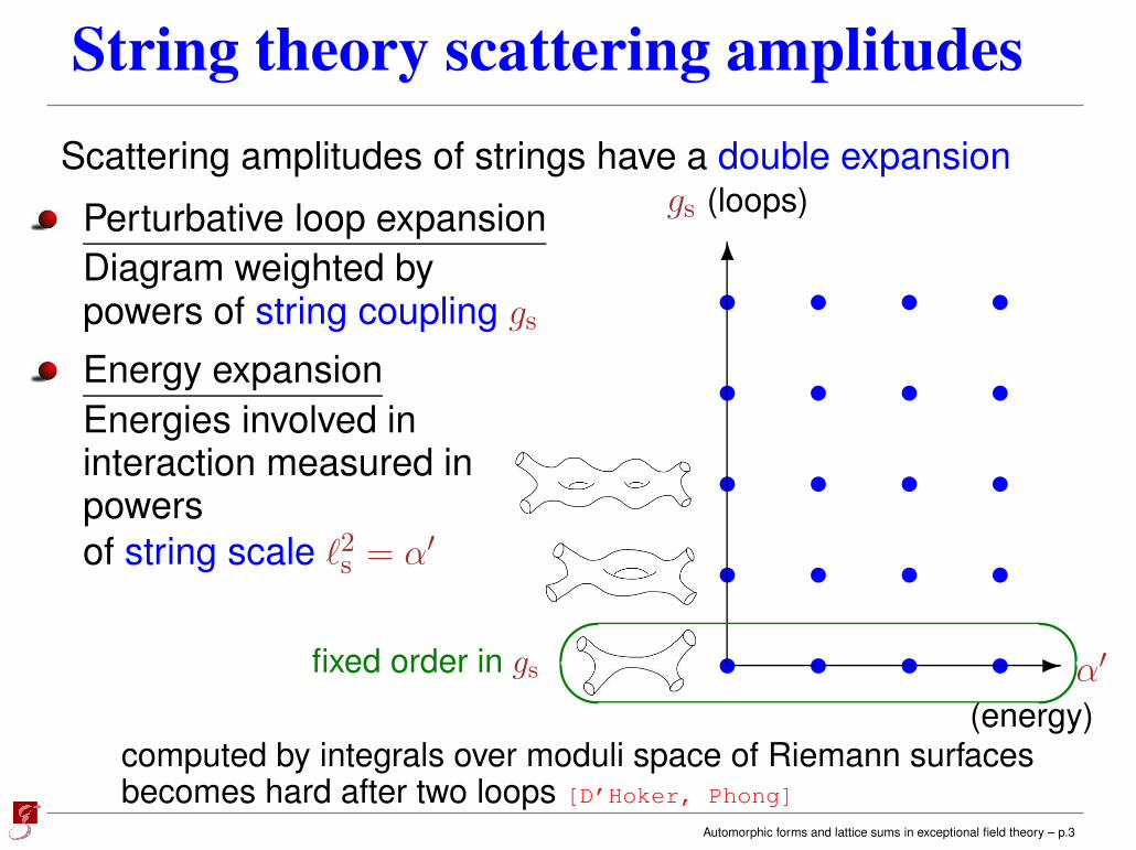
Scattering amplitudes of strings have a double expansion
ttttt
ttttt
ttttt
ttttt
gs (loops)
α′
(energy)
Perturbative loop expansion
Diagram weighted bypowers of string coupling gs
Energy expansion
Energies involved ininteraction measured inpowers
of string scale ℓ2s = α′
Automorphic forms and lattice sums in exceptional field theory – p.3
String theory scattering amplitudes
Scattering amplitudes of strings have a double expansion
ttttt
ttttt
ttttt
ttttt
gs (loops)
α′
(energy)
Perturbative loop expansion
Diagram weighted bypowers of string coupling gs
Energy expansion
Energies involved ininteraction measured inpowers
of string scale ℓ2s = α′
fixed order in gs
computed by integrals over moduli space of Riemann surfacesbecomes hard after two loops [D’Hoker, Phong]
Automorphic forms and lattice sums in exceptional field theory – p.3

String theory scattering amplitudes
Scattering amplitudes of strings have a double expansion
ttttt
ttttt
ttttt
ttttt
gs (loops)
α′
(energy)
Perturbative loop expansion
Diagram weighted bypowers of string coupling gs
Energy expansion
Energies involved ininteraction measured inpowers
of string scale ℓ2s = α′
incl. non-pert.
(up to) fixed energy order
sometimes fixed by (discrete) symmetries/automorphyAutomorphic forms and lattice sums in exceptional field theory – p.3
String theory effective action
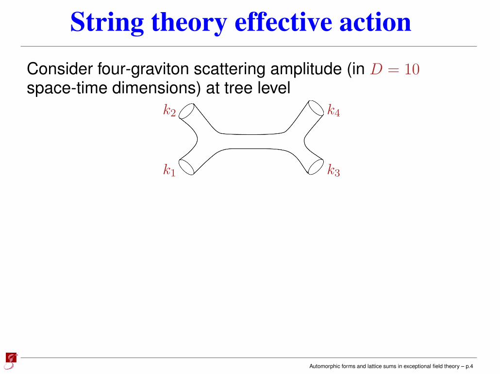
Consider four-graviton scattering amplitude (in D = 10space-time dimensions) at tree level
k1
k2
k3
k4
Automorphic forms and lattice sums in exceptional field theory – p.4

String theory effective action
Consider four-graviton scattering amplitude (in D = 10space-time dimensions) at tree level
k1
k2
k3
k4
Atree(s, t, u) = g−2s
4
stu
Γ(1− α′s)Γ(1− α′t)Γ(1− α′u)
Γ(1 + α′s)Γ(1 + α′t)Γ(1 + α′u)R4
Automorphic forms and lattice sums in exceptional field theory – p.4

String theory effective action
Consider four-graviton scattering amplitude (in D = 10space-time dimensions) at tree level
k1
k2
k3
k4
Atree(s, t, u) = g−2s
4
stu
Γ(1− α′s)Γ(1− α′t)Γ(1− α′u)
Γ(1 + α′s)Γ(1 + α′t)Γ(1 + α′u)R4
Mandelstam
variables
s = −(k1 + k2)2
t = −(k1 + k4)2
u = −(k1 + k3)2
string coupling:
tree level
absorbs polarisation
tensors
α′ = ℓ2s
string scale
Expand for low energies
α′s << 1, α′t << 1 and α′u << 1
Automorphic forms and lattice sums in exceptional field theory – p.4

String theory effective action
Consider four-graviton scattering amplitude (in D = 10space-time dimensions) at tree level
k1
k2
k3
k4
Atree(s, t, u) = g−2s
4
stu
Γ(1− α′s)Γ(1− α′t)Γ(1− α′u)
Γ(1 + α′s)Γ(1 + α′t)Γ(1 + α′u)R4
= 4g−2s R4
[1
stu+ (α′)3·2ζ(3)+(α′)5(s2 + t2 + u2)·ζ(5)+ . . .
]
dimensionful
Automorphic forms and lattice sums in exceptional field theory – p.4

Low energy effective action
Gravitational interaction at lowest energies in D space-timedimensions normally described by general relativity (orsupergravity) with Lagrangian
L = ℓ2−DRlength scale ∼
√α′
Riemann scalar
curvature of space-time
two-derivatives
Automorphic forms and lattice sums in exceptional field theory – p.5

Low energy effective action
Gravitational interaction at lowest energies in D space-timedimensions normally described by general relativity (orsupergravity) with Lagrangian
L = ℓ2−DRlength scale ∼
√α′
Riemann scalar
curvature of space-time
two-derivatives
Higher orders in α′ are related to higher derivativemodifications. For gravity in D dimensions schematicallyfrom string tree level (Einstein frame)
e−1L= ℓ2−DR + ℓ8−D2ζ(3)g−3/2s R4
+ℓ12−Dζ(5)g−5/2s ∇4R4 + . . .
Automorphic forms and lattice sums in exceptional field theory – p.5

Low energy effective action
Gravitational interaction at lowest energies in D space-timedimensions normally described by general relativity (orsupergravity) with Lagrangian
L = ℓ2−DRlength scale ∼
√α′
Riemann scalar
curvature of space-time
two-derivatives
Higher orders in α′ are related to higher derivativemodifications. For gravity in D dimensions schematicallyfrom string tree level (Einstein frame)
e−1L= ℓ2−DR + ℓ8−D2ζ(3)g−3/2s R4
+ℓ12−Dζ(5)g−5/2s ∇4R4 + . . . t
tttt
ttttt
ttttt
ttttt
gs (loops)
α′
(energy)
2ζ(3)
ζ(5)
Automorphic forms and lattice sums in exceptional field theory – p.5

Moduli fields and U-duality (I)
The string coupling gs is a modulus of string theory.
Moduli contain information of the background on whichstrings propagate.
Automorphic forms and lattice sums in exceptional field theory – p.6

Moduli fields and U-duality (I)
The string coupling gs is a modulus of string theory.
Moduli contain information of the background on whichstrings propagate.
Other moduli: For toroidal backgrounds including
T d−1 = (S1)d−1 the radii are also moduli
R
momentum n
winding w
1R
R ↔ 1
R
n ↔ w
momentum wwinding n
Equivalent string theories! T-duality SO(d− 1, d− 1,Z)
Automorphic forms and lattice sums in exceptional field theory – p.6

Moduli fields and U-duality (II)
On gs and (RR) axion χ action of SL(2,Z) S-duality
z = χ+ ig−1s
(
a b
c d
)
· z =az + b
cz + d
giving equivalent string theories. z ∈ SL(2,R)/SO(2)
Automorphic forms and lattice sums in exceptional field theory – p.7

Moduli fields and U-duality (II)
On gs and (RR) axion χ action of SL(2,Z) S-duality
z = χ+ ig−1s
(
a b
c d
)
· z =az + b
cz + d
giving equivalent string theories. z ∈ SL(2,R)/SO(2)
All moduli g together form moduli space M [Hull, Townsend
1995]
g ∈ M = Ed(Z)\Ed(d)/K(Ed)
U-duality Cremmer–Juliahidden symmetry
compact subgp
t t t tt t1
2
3 4 5 dAutomorphic forms and lattice sums in exceptional field theory – p.7

Moduli fields and U-duality (II)
On gs and (RR) axion χ action of SL(2,Z) S-duality
z = χ+ ig−1s
(
a b
c d
)
· z =az + b
cz + d
giving equivalent string theories. z ∈ SL(2,R)/SO(2)
All moduli g together form moduli space M [Hull, Townsend
1995]
g ∈ M = Ed(Z)\Ed(d)/K(Ed)
U-duality Cremmer–Juliahidden symmetry
compact subgp
t t t tt t1
2
3 4 5 d
T-dualityS-duality
Automorphic forms and lattice sums in exceptional field theory – p.7

Coefficient functions in amplitude (I)
Expand the (analytic part of the) full scattering amplitude inenergy direction
A(s, t, u; g) = R4
1
stu+∑
p,q≥0
E(p,q)(g)σp2σq3
with σn =(α′)n
4n (sn + tn + un) and g ∈ M. ttttt
ttttt
ttttt
ttttt
gs (loops)
α′
(energy)
E(0,0) E(1,0)
Automorphic forms and lattice sums in exceptional field theory – p.8

Coefficient functions in amplitude (I)
Expand the (analytic part of the) full scattering amplitude inenergy direction
A(s, t, u; g) = R4
1
stu+∑
p,q≥0
E(p,q)(g)σp2σq3
with σn =(α′)n
4n (sn + tn + un) and g ∈ M. ttttt
ttttt
ttttt
ttttt
gs (loops)
α′
(energy)
E(0,0) E(1,0)
Coefficient functions E(p,q)are invariant under U-duality Ed(Z)
are of moderate growth in order to be compatible withperturbation theory
satisfy differential equations for supersymmetry
⇒ Looking for (spherical) automorphic forms on EdAutomorphic forms and lattice sums in exceptional field theory – p.8

Coefficient functions in amplitude (II)
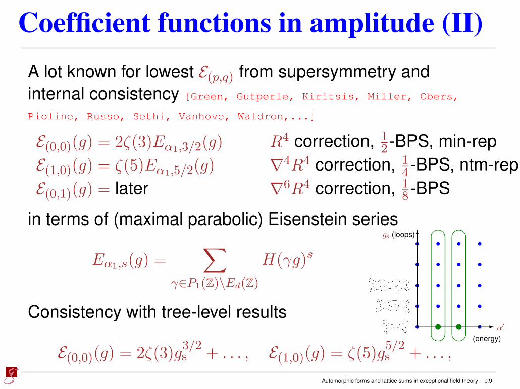
A lot known for lowest E(p,q) from supersymmetry and
internal consistency [Green, Gutperle, Kiritsis, Miller, Obers,
Pioline, Russo, Sethi, Vanhove, Waldron,...]
E(0,0)(g) = 2ζ(3)Eα1,3/2(g) R4 correction, 12-BPS, min-rep
E(1,0)(g) = ζ(5)Eα1,5/2(g) ∇4R4 correction, 14-BPS, ntm-rep
E(0,1)(g) = later ∇6R4 correction, 18-BPS
in terms of (maximal parabolic) Eisenstein series
Eα1,s(g) =∑
γ∈P1(Z)\Ed(Z)
H(γg)s
Automorphic forms and lattice sums in exceptional field theory – p.9
Coefficient functions in amplitude (II)
A lot known for lowest E(p,q) from supersymmetry and
internal consistency [Green, Gutperle, Kiritsis, Miller, Obers,
Pioline, Russo, Sethi, Vanhove, Waldron,...]
E(0,0)(g) = 2ζ(3)Eα1,3/2(g) R4 correction, 12-BPS, min-rep
E(1,0)(g) = ζ(5)Eα1,5/2(g) ∇4R4 correction, 14-BPS, ntm-rep
E(0,1)(g) = later ∇6R4 correction, 18-BPS
in terms of (maximal parabolic) Eisenstein series
Eα1,s(g) =∑
γ∈P1(Z)\Ed(Z)
H(γg)s
ttttt
ttttt
ttttt
ttttt
gs (loops)
α′
(energy)
Consistency with tree-level results
E(0,0)(g) = 2ζ(3)g3/2s + . . . , E(1,0)(g) = ζ(5)g
5/2s + . . . ,
Automorphic forms and lattice sums in exceptional field theory – p.9
Different viewpoint: Field theory
Instead of reviewing Fourier expansions and consistency ofanswers above [Green, Miller, Russo, Vanhove; Obers, Pioline;...]
⇒ use that four-graviton process is very special. Low
order corrections R4, ∇4R4 and ∇6R4 are partially BPS
=⇒ Only BPS states contribute; no other string theorystates visible at low energies
Automorphic forms and lattice sums in exceptional field theory – p.10
Different viewpoint: Field theory
Instead of reviewing Fourier expansions and consistency ofanswers above [Green, Miller, Russo, Vanhove; Obers, Pioline;...]
⇒ use that four-graviton process is very special. Low
order corrections R4, ∇4R4 and ∇6R4 are partially BPS
=⇒ Only BPS states contribute; no other string theorystates visible at low energies
Used by [Green, Vanhove] to perform supergravity loopcalculations including BPS momentum states to find E(0,0)and E(1,0) in D = 10 dimensions.
Automorphic forms and lattice sums in exceptional field theory – p.10

Different viewpoint: Field theory
Instead of reviewing Fourier expansions and consistency ofanswers above [Green, Miller, Russo, Vanhove; Obers, Pioline;...]
⇒ use that four-graviton process is very special. Low
order corrections R4, ∇4R4 and ∇6R4 are partially BPS
=⇒ Only BPS states contribute; no other string theorystates visible at low energies
Used by [Green, Vanhove] to perform supergravity loopcalculations including BPS momentum states to find E(0,0)and E(1,0) in D = 10 dimensions.
Aim: Investigate E(p,q) for D < 10 by similar methods in
manifestly U-duality covariant formalism
=⇒ Exceptional field theory loops
Automorphic forms and lattice sums in exceptional field theory – p.10

Exceptional field theory
[de Wit, Nicolai; Hull; Waldram et al.;
Hohm, Samtleben; West; ...] t t t tt1 3 4 d
2 Ed
Formalism to make hidden Ed(R) (continuous!) manifest.
Consider extended space-time (D = 11− d)
MD ×Md(αd)
Coordinates xµ, yM with µ = 0, ..., D − 1 and M = 1, ..., d(αd).
d(αd) = dimRαd: hst. weight rep. on node αd
Automorphic forms and lattice sums in exceptional field theory – p.11

Exceptional field theory
[de Wit, Nicolai; Hull; Waldram et al.;
Hohm, Samtleben; West; ...] t t t tt1 3 4 d
2 Ed
Formalism to make hidden Ed(R) (continuous!) manifest.
Consider extended space-time (D = 11− d)
MD ×Md(αd)
Coordinates xµ, yM with µ = 0, ..., D − 1 and M = 1, ..., d(αd).
d(αd) = dimRαd: hst. weight rep. on node αd
Rαddecomposes under ‘gravity line’ GL(d,R) ⊂ Ed(R)
yM = (ym, y[mn], y[m1...m5], . . .) (m,n, ... = 1, ..., d)
KK momenta❨M2 wrappings
Automorphic forms and lattice sums in exceptional field theory – p.11
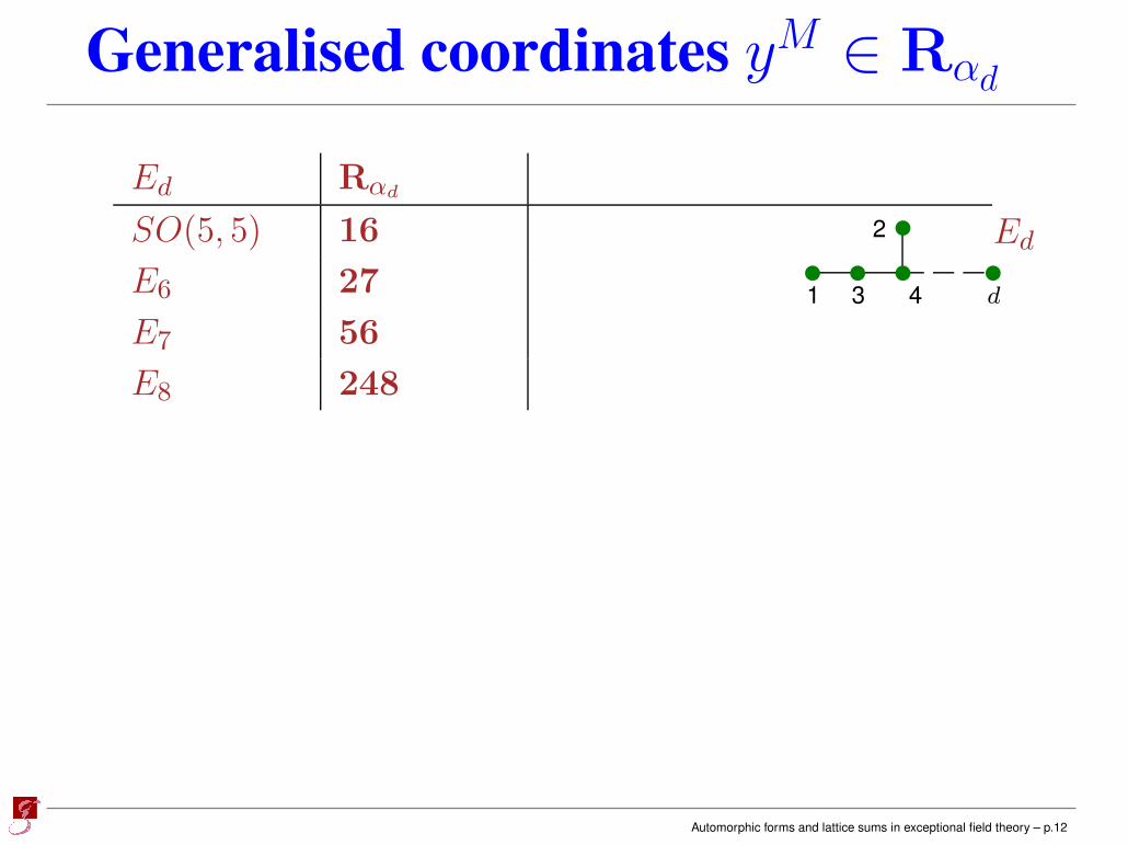
Generalised coordinates yM ∈ Rαd
t t t tt1 3 4 d
2 Ed
Ed Rαd
SO(5, 5) 16
E6 27
E7 56
E8 248
Automorphic forms and lattice sums in exceptional field theory – p.12

Generalised coordinates yM ∈ Rαd
t t t tt1 3 4 d
2 Ed
Ed RαdRα1
SO(5, 5) 16 10
E6 27 27
E7 56 133
E8 248 3875⊕ 1
Generalised coordinates yM have to obey section constraint
∂A
∂yM∂B
∂yN
∣∣∣∣Rα1
= 0
for any two fields A(xµ, yM ), B(xµ, yM ). LHS belongs to
Rαd⊗Rαd
= Rα1 ⊕ . . .
Automorphic forms and lattice sums in exceptional field theory – p.12
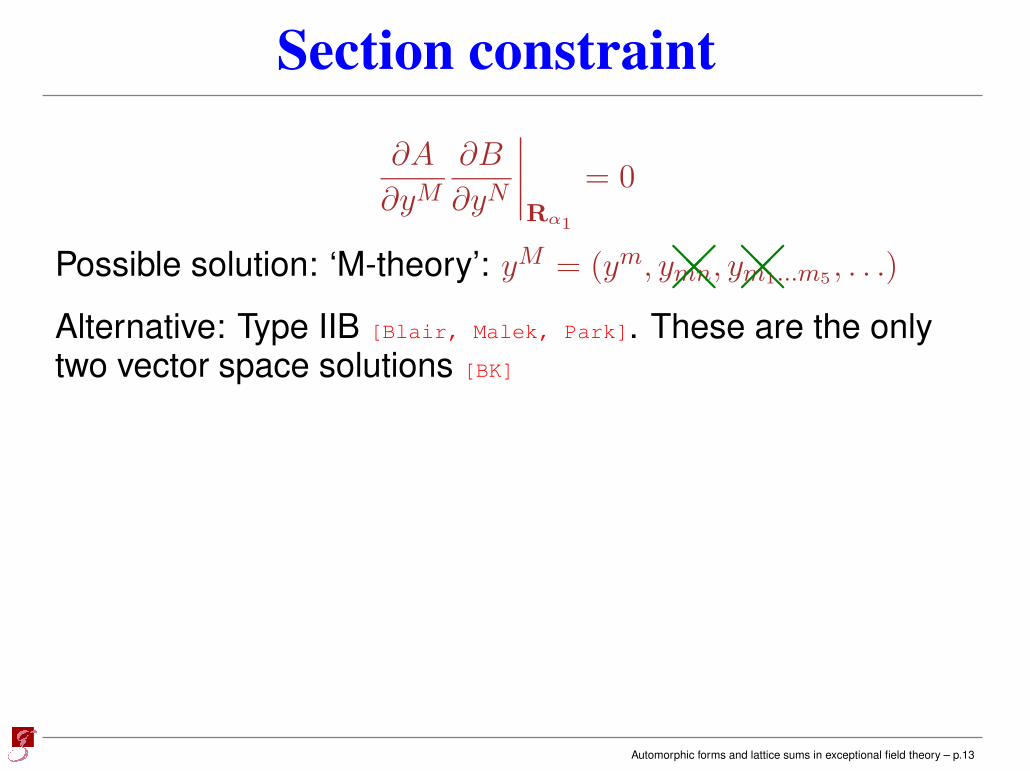
Section constraint
∂A
∂yM∂B
∂yN
∣∣∣∣Rα1
= 0
Possible solution: ‘M-theory’: yM = (ym, ymn, ym1...m5 , . . .)
Alternative: Type IIB [Blair, Malek, Park]. These are the onlytwo vector space solutions [BK]
Automorphic forms and lattice sums in exceptional field theory – p.13

Section constraint
∂A
∂yM∂B
∂yN
∣∣∣∣Rα1
= 0
Possible solution: ‘M-theory’: yM = (ym, ymn, ym1...m5 , . . .)
Alternative: Type IIB [Blair, Malek, Park]. These are the onlytwo vector space solutions [BK]
Here: ‘Toroidal’ extended space for yM . Conjugatemomenta are quantised charges
ΓM = (nm, nm1m2 , nn1...n5 , . . .) ∈ Z
d(αd)
Section constraint becomes 12-BPS constraint on charges
Γ× Γ∣∣Rα1
= 0 ⇒ write Γ× Γ = 0 for brevity
−→ One loop Automorphic forms and lattice sums in exceptional field theory – p.13

Amplitudes in EFT (I)
Exceptional field theory is mainly a classical theory. QFTtreatment complicated due to section constraint.
Consider 3-point vertex in EFT φ ∂φ ∂φ
∫
R11−d
dx
∫
Rd(αd)/section
dy φ(x, y) (∇φ(x, y) · ∇φ(x, y))
Automorphic forms and lattice sums in exceptional field theory – p.14

Amplitudes in EFT (I)
Exceptional field theory is mainly a classical theory. QFTtreatment complicated due to section constraint.
Consider 3-point vertex in EFT φ ∂φ ∂φ
∫
R11−d
dx
∫
Rd(αd)/section
dy φ(x, y) (∇φ(x, y) · ∇φ(x, y))
y-Fourier expand φ(x, y) =∑
Γ∈Zd(αd)
φΓ(x)eiℓ−1Γ·y. Vertex
∑
Γ1,Γ2∈Zd(αd)
Γ1×Γ2=0
∫
R11−d
dxφ−Γ1−Γ2(x)[
∂µφΓ1∂µφΓ2
−ℓ−2 〈Z(Γ1)|Z(Γ2)〉φΓ1φΓ2
]
︸ ︷︷ ︸charge dependent mass
Section constraint on yM turned into constraint on charges
Automorphic forms and lattice sums in exceptional field theory – p.14

Amplitudes in EFT (II)
〈Z(Γ)|Z(Γ)〉 like BPS-mass. In M-theory frame
ds211 = e9−d3
φMmndymdyn + e−
d3φηµνdx
µdxν
φ now dilaton; Mmn uni-modular metric on T d.
|Z(Γ)|2 = e−3φMmnnmnn+1
2e(6−d)φMm1n1Mm2n2n
m1m2nn1n2+. . .
From form of vertex see that momenta in propagators areeffectively shifted by Kaluza–Klein mass
p2 −→ p2 + ℓ−2|Z(Γ)|2
and section constraint Γi × Γj = 0 at every vertex.
Automorphic forms and lattice sums in exceptional field theory – p.15
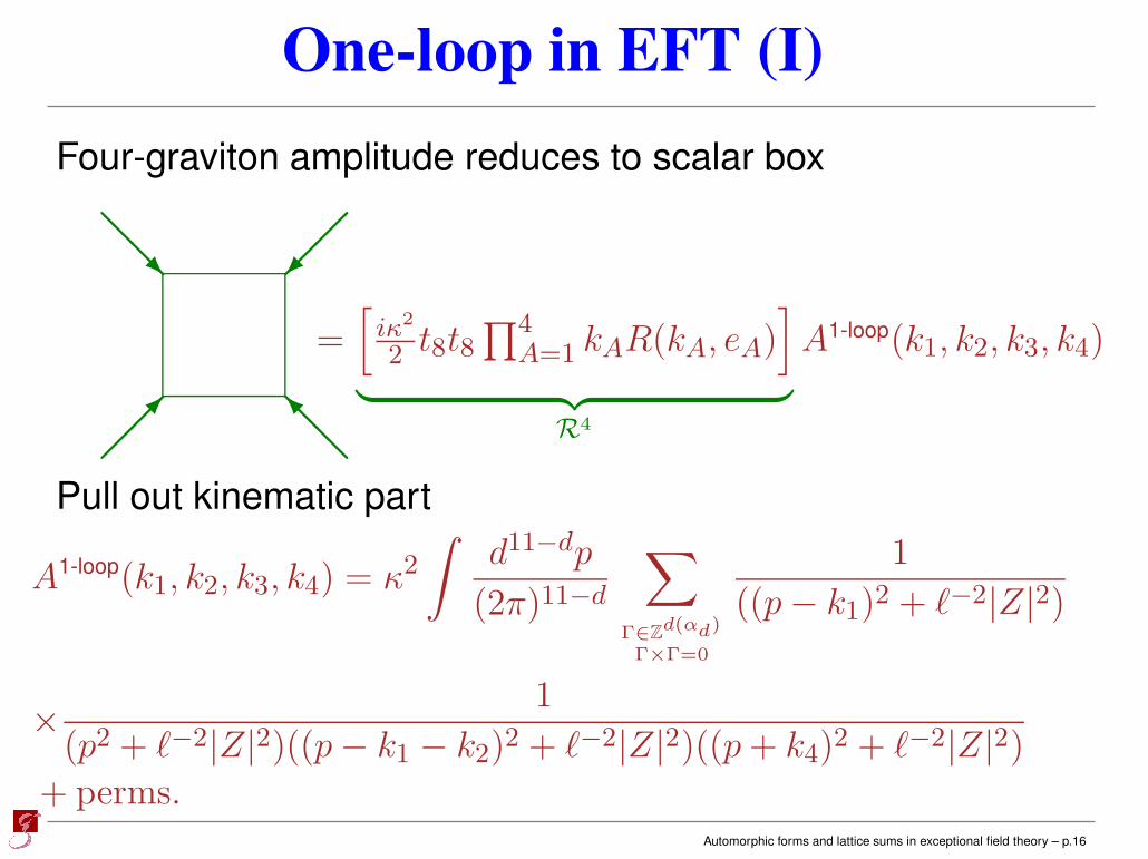
One-loop in EFT (I)
Four-graviton amplitude reduces to scalar box
=[iκ2
2 t8t8∏4
A=1 kAR(kA, eA)]
A1-loop(k1, k2, k3, k4)
︸ ︷︷ ︸
R4
Pull out kinematic part
A1-loop(k1, k2, k3, k4) = κ2∫
d11−dp
(2π)11−d
∑
Γ∈Zd(αd)
Γ×Γ=0
1
((p− k1)2 + ℓ−2|Z|2)
× 1
(p2 + ℓ−2|Z|2)((p− k1 − k2)2 + ℓ−2|Z|2)((p+ k4)2 + ℓ−2|Z|2)+ perms.
Automorphic forms and lattice sums in exceptional field theory – p.16

One-loop in EFT (II)
Γ = 0 term corresponds to SUGRA in D = 11− d; usual logthreshold contribution ⇒ remove for analytic eff. action
Treat loop integral over d11−dp with usual Schwinger andFeynman techniques:
A1-loop(k1, k2, k3, k4) = 4πℓ9−d∑
Γ∈Zd(αd)
Γ×Γ=0
∞∫
0
dv
vd−12
1∫
0
dx1
x1∫
0
dx2
x2∫
0
dx3
× exp[π
v
((1− x1)(x2 − x3)s+ x3(x1 − x2)t− ℓ−2|Z|2
)]
+ perms.
Low energy from expanding in Mandelstam variables
s = −(k1 + k2)2, t = −(k1 + k4)
2, u = −(k1 + k3)2.
Automorphic forms and lattice sums in exceptional field theory – p.17

Low energy correction terms
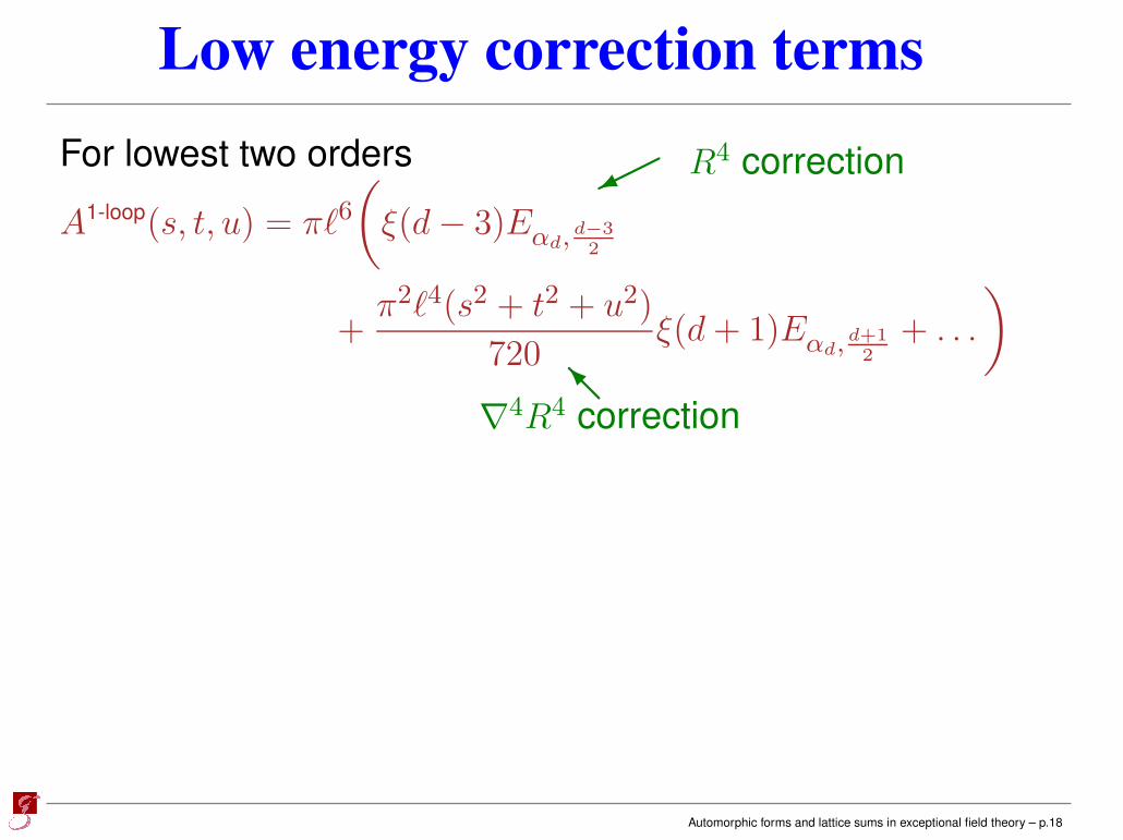
For lowest two orders
A1-loop(s, t, u) = πℓ6(
ξ(d− 3)Eαd,d−32
+π2ℓ4(s2 + t2 + u2)
720ξ(d+ 1)Eαd,
d+12
+ . . .
)
Automorphic forms and lattice sums in exceptional field theory – p.18
Low energy correction terms
For lowest two orders
A1-loop(s, t, u) = πℓ6(
ξ(d− 3)Eαd,d−32
+π2ℓ4(s2 + t2 + u2)
720ξ(d+ 1)Eαd,
d+12
+ . . .
)
R4 correction
∇4R4 correction
Automorphic forms and lattice sums in exceptional field theory – p.18

Low energy correction terms
For lowest two orders
A1-loop(s, t, u) = πℓ6(
ξ(d− 3)Eαd,d−32
+π2ℓ4(s2 + t2 + u2)
720ξ(d+ 1)Eαd,
d+12
+ . . .
)
R4 correction
∇4R4 correction
Notation
ξ(s) = π−s/2Γ(s/2)ζ(s) [completed Riemann zeta]
Eαd,s =1
2ζ(2s)
∑
Γ 6=0Γ×Γ=0
|Z(Γ)|−2s [Eisenstein series]
Restricted lattice sum rewritable as single U-duality orbit!−→ Two loops −→ Beyond
Automorphic forms and lattice sums in exceptional field theory – p.18
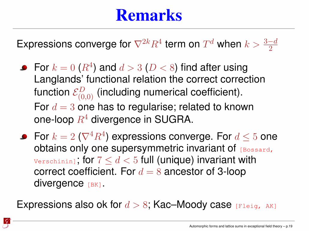
Remarks
Expressions converge for ∇2kR4 term on T d when k > 3−d2
For k = 0 (R4) and d > 3 (D < 8) find after usingLanglands’ functional relation the correct correction
function ED(0,0) (including numerical coefficient).
For d = 3 one has to regularise; related to known
one-loop R4 divergence in SUGRA.
For k = 2 (∇4R4) expressions converge. For d ≤ 5 oneobtains only one supersymmetric invariant of [Bossard,
Verschinin]; for 7 ≤ d < 5 full (unique) invariant withcorrect coefficient. For d = 8 ancestor of 3-loopdivergence [BK].
Expressions also ok for d > 8; Kac–Moody case [Fleig, AK]
Automorphic forms and lattice sums in exceptional field theory – p.19

Two loops in EFT (I)
Automorphic forms and lattice sums in exceptional field theory – p.20

Two loops in EFT (I)
[Bern et al.]: combination of planar and non-planar scalardiagram at L = 2
After a few pages of calculation
A2-loop(s, t, u) ∼ ℓ6∑
Γ1,Γ2Γi×Γj=0
∫ ∞
0
d3Ω
(detΩ)7−d2
e−Ωij〈Z(Γi)|Z(Γj)〉
×[ℓ4(s2 + t2 + u2)
6+
ℓ6(s3 + t3 + u3)
72Φ(0,1)(Ω) + . . .
]
∇4R4 correction
∇6R4
Automorphic forms and lattice sums in exceptional field theory – p.20

Two loops in EFT (II)
Focus first on ∇4R4 contribution. Need to understand
∑
Γ1,Γ2Γi×Γj=0
∫ ∞
0
d3Ω
(detΩ)7−d2
e−Ωij〈Z(Γi)|Z(Γj)〉
where Ωij = Ω =
(
L1 + L3 L3
L3 L2 + L3
)
Automorphic forms and lattice sums in exceptional field theory – p.21

Two loops in EFT (II)
Focus first on ∇4R4 contribution. Need to understand
∑
Γ1,Γ2Γi×Γj=0
∫ ∞
0
d3Ω
(detΩ)7−d2
e−Ωij〈Z(Γi)|Z(Γj)〉
where Ωij = Ω =
(
L1 + L3 L3
L3 L2 + L3
)
Sum is restricted to pairs of charges Γ1, Γ2 satisfying
Γi × Γj |Rα1= 0
Solutions can be parametrised by suitable parabolicdecompositions [BK].
Automorphic forms and lattice sums in exceptional field theory – p.21

Two loops in EFT (III)
Putting everything together
A2-loop,∇4R4
(s, t, u) = 8πℓ10ξ(d− 4)ξ(d− 5)Eαd−1,d−42
This gives the correct function and coefficient for3 ≤ d ≤ 8 with the right coefficient. Case d = 5 (D = 6)trickier due to IR divergences.
Certain doubling of contributions from one loop and twoloops. Corrected if one-loop result renormalised.
Other orbits of M subdominant at low energies exceptd = 5.
Automorphic forms and lattice sums in exceptional field theory – p.22

Beyond Eisenstein series (I)
Consider ∇6R4 term E(0,1). Inhomogeneous equation [Green,
Vanhove]
(∆− λ)E(0,1) = −E2(0,0)
Poisson equation. Not Eisenstein series!
Automorphic forms and lattice sums in exceptional field theory – p.23

Beyond Eisenstein series (I)
Consider ∇6R4 term E(0,1). Inhomogeneous equation [Green,
Vanhove]
(∆− λ)E(0,1) = −E2(0,0)
Poisson equation. Not Eisenstein series!
Recently solved in D = 10 dimensions (SL(2,Z)) by [Green,
Miller, Vanhove], giving correct perturbative results.
For other dimensions can write Poincaré series form [Ahlen,
AK in progress] that needs to be studied further.
E(0,1)(g) =∑
γ∈P1\Ed
σ(γg)
with σ(g) not a character on P1 but depends on unipotentpart through Bessel functions. −→ yonder
Automorphic forms and lattice sums in exceptional field theory – p.23

Beyond Eisenstein series (II)
Using exceptional field theory can also find a solution
E2-loop(0,1)
=2π5−d
9
∑
Γi∈Z2d(αd)∗
Γi×Γj=0
∫
R×3+
d3Ω
(detΩ)7−d2
(
L1 + L2 + L3 − 5L1L2L3
detΩ
)
e−Ωij〈Z(Γi)|Z(Γj)〉
Resembles an independent string theory answer based onthe Zhang–Kawazumi invariant [Pioline].
More general questions
Space of functions required for solving inhomogeneousLaplace equation?
Automorphic distributions?
Fourier expansion and wavefront set?
Automorphic representations? Global picture?
Automorphic forms and lattice sums in exceptional field theory – p.24

Summary and outlook
Explicitly evaluated loop amplitudes in EFT
Reproduced known E(p,q) in
manifestly U-duality covariant form
Useful tools for dealing with sectionconstraint
Analysis of differential equation forhigher order corrections and theirwavefront sets
Hasse diagram for E7(7)
0
A1
2A1
(3A1)′
(3A1)′′
A2
4A1
A1A2
R
R4
∇4R4
∇6R4
∇6R4
Automorphic forms and lattice sums in exceptional field theory – p.25
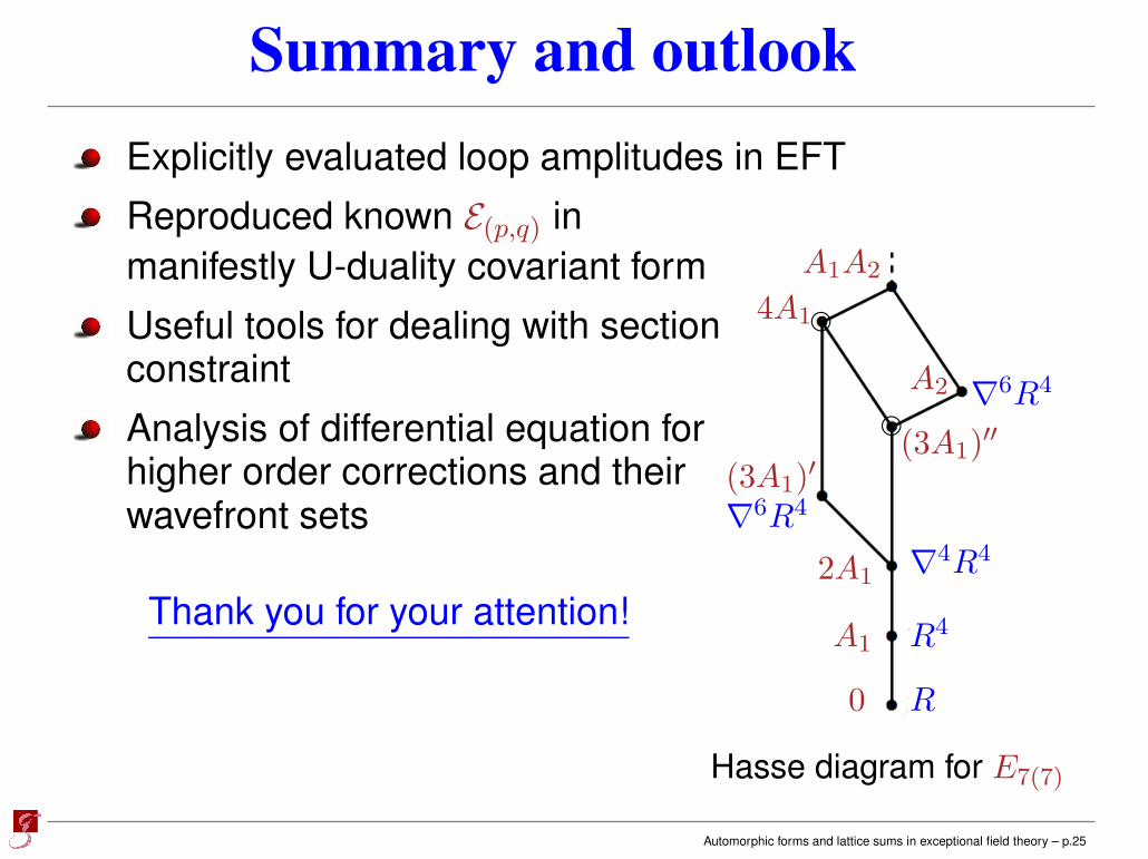
Summary and outlook
Explicitly evaluated loop amplitudes in EFT
Reproduced known E(p,q) in
manifestly U-duality covariant form
Useful tools for dealing with sectionconstraint
Analysis of differential equation forhigher order corrections and theirwavefront sets
Hasse diagram for E7(7)
0
A1
2A1
(3A1)′
(3A1)′′
A2
4A1
A1A2
R
R4
∇4R4
∇6R4
∇6R4
Thank you for your attention!
Automorphic forms and lattice sums in exceptional field theory – p.25

Beyond Eisenstein (III)
Solve (∆− 12)f(z) = −4ζ(3)E3/2(z)2: [Green, Miller, Vanhove]
f(z) =∑
γ∈Γ∞\SL(2,Z)
σ(γz), where (z = x+ iy) and
σ(z) = 2ζ(3)2y3 +1
9π2y +
∑
n 6=0
cn(y)e2πinx
cn(y) = 8ζ(3)σ−2(n)y
[(
1 +10
π2n2y2
)
K0(2π|n|y)
+
(6
π|n|y +10
π3|n|3y3)
K1(2π|n|y)−16
π(|n|y)1/2K7/2(2π|n|y)
]
For higher rank U-dualities (in progress with Olof Ahlén).
Automorphic forms and lattice sums in exceptional field theory – p.26

Kac–Moody questions
K-types
For discrete series often non-trivial K-types necessary.Possibilities for Kac–Moody?
Automorphic forms and lattice sums in exceptional field theory – p.27

Kac–Moody questions
K-types
For discrete series often non-trivial K-types necessary.Possibilities for Kac–Moody?
At the level of Lie algebras k ⊂ g over R.
(1) ∞-dim’l fixed point Lie algebra of (Chevalley) involution.(2) k is not a Kac–Moody algebra.(3) k is not a simple algebra. It has ∞-dim’l ideals.
Automorphic forms and lattice sums in exceptional field theory – p.27
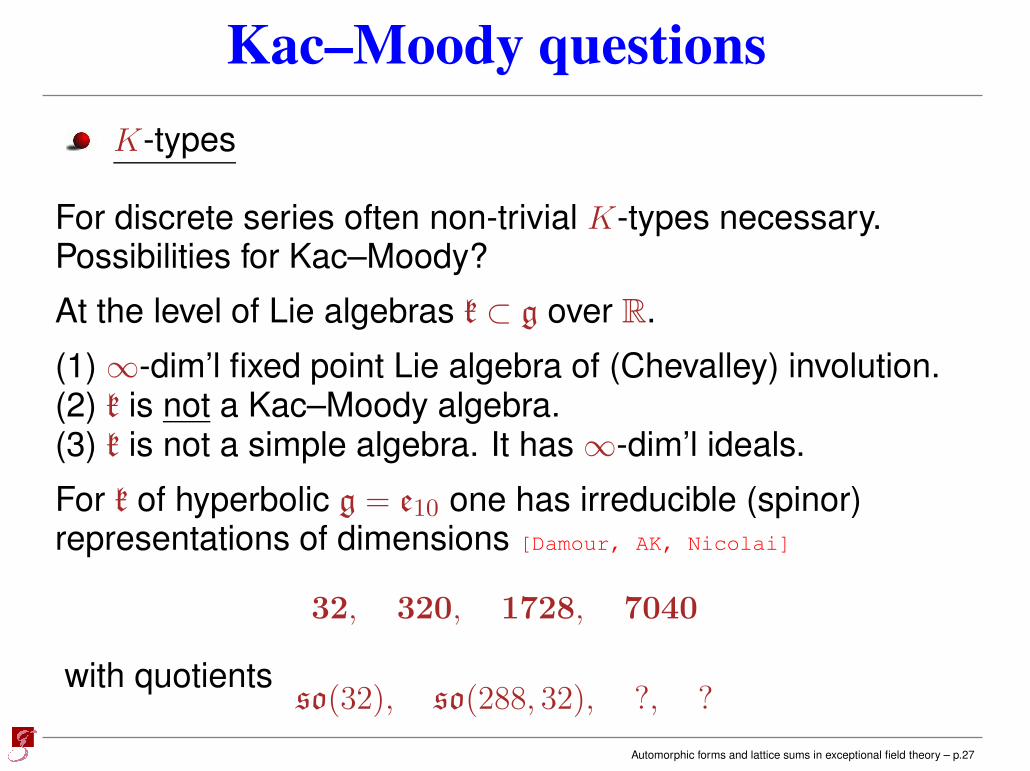
Kac–Moody questions
K-types
For discrete series often non-trivial K-types necessary.Possibilities for Kac–Moody?
At the level of Lie algebras k ⊂ g over R.
(1) ∞-dim’l fixed point Lie algebra of (Chevalley) involution.(2) k is not a Kac–Moody algebra.(3) k is not a simple algebra. It has ∞-dim’l ideals.
For k of hyperbolic g = e10 one has irreducible (spinor)representations of dimensions [Damour, AK, Nicolai]
32, 320, 1728, 7040
with quotientsso(32), so(288, 32), ?, ?
Automorphic forms and lattice sums in exceptional field theory – p.27
K-types
(Some of) these representations can be lifted to the Weylgroup W and (covers of) K [Ghatei, Horn, Kohl, Weiss].
Question: Can they arise as K-types of some Grepresentations?
Automorphic forms and lattice sums in exceptional field theory – p.28

K-types
(Some of) these representations can be lifted to the Weylgroup W and (covers of) K [Ghatei, Horn, Kohl, Weiss].
Question: Can they arise as K-types of some Grepresentations?
For other Kac–Moody groups, e.g.
2 −2
−2 2 −1
−1 2
other
quotients possible, also with U(1) factors⇒ holomorphic discrete series?
Question: Spherical vectors for Kac–Moody reps?
Automorphic forms and lattice sums in exceptional field theory – p.28


![IS THERE AN ANALYTIC THEORY OF AUTOMORPHIC FUNCTIONS …frenkel/analytic.pdf · IS THERE A THEORY OF AUTOMORPHIC FUNCTIONS FOR COMPLEX CURVES? 5 In [L2] an attempt is made to explicitly](https://static.documents.pub/doc/80x56/5f03950f7e708231d409c353/is-there-an-analytic-theory-of-automorphic-functions-frenkelanalyticpdf-is-there.jpg)


