
Capacity Expansion for Random Exponential Demand Growth with Lead Times
Sarah M. Ryan
Department of Industrial and Manufacturing Systems Engineering Iowa State University Ames, IA 50011-2164
Phone: 515-294-4347 Fax: 515-294-3524
October, 2003
Working Paper: Results not to be used or quoted without permission of the author.
For publication in Management Science.
Capacity Expansion for Random Exponential Demand Growth
Abstract
The combination of demand uncertainty and a lead time for adding capacity
creates the risk of capacity shortage during the lead time. We formulate a model
of capacity expansion for uncertain exponential demand growth and deterministic
expansion lead times when there is an obligation to provide a specified level of
service. The service level, defined in terms of the ratio of expected lead time
shortage to installed capacity, is guaranteed by timing each expansion to begin
when demand reaches a fixed proportion of the capacity position. Under this
timing rule, the optimal facilities to install can be determined by solving an
equivalent deterministic problem without lead times. Numerical results show the
effects of the demand parameters and lead time length on the expansion timing.
The interaction of timing with expansion size is explored for the case when
continuous facility sizes are available with economies of scale.
1
1. Introduction
When demand for capacity is uncertain and significant lead times exist for adding capacity,
managers must carefully consider the sizes and timing of new capacity additions. Discounting
future costs encourages the delay of capacity expansion to the latest possible moment. However,
when demand is expected to grow, postponing capacity additions increases the risk of capacity
shortage during the installation lead time. Economies of scale also work in opposition to
future cost discounting to encourage larger capacity increments. This paper describes a capacity
expansion model in which installation lead times are fixed and the only source of uncertainty is
the demand for capacity. The expected growth in demand follows an exponential trend. The
study is most relevant to service providers who have some obligation to maintain sufficient
capacity for their subscribers and therefore wish to avoid shortages. Even if an expansion is
initiated while excess capacity remains, there is a risk of running short of capacity during the
installation lead time. In this paper we develop a timing policy to provide a specified level of
service and show how its parameter can be obtained numerically. Under this timing policy, the
capacity additions that minimize the infinite horizon expected discounted cost can be identified
by solving an equivalent deterministic problem without lead times.
Exponential growth in demand for capacity may occur in rapidly growing industries or
economies. For example, forecasts of the growth in Internet hosts (Rai et al. 1998) and
connections (Bieler and Stevenson 1998) predicted an exponential increase in the global size of
the Internet. Srinivasan (1967) formulated a model with deterministic geometric growth for
heavy industries in India assuming a continuum of possible expansions and proved that under a
specific economies of scale assumption, the infinite horizon discounted cost is minimized by
expanding capacity at regular time intervals, a result also proved by Sinden (1960). If demand is
2
uncertain but lead times are negligible, then the timing of capacity additions can follow the
realization of demand growth. Smith (1979) proved a turnpike theorem and developed an
algorithm for solving the problem with deterministic exponential demand growth and discrete
facilities. Bean, Higle and Smith (1992) modeled demand as either a transformation of
Brownian motion with drift or a semi-Markovian birth and death process. They derived an
equivalent deterministic formulation that showed that the effect of uncertainty is to lower the
interest rate, so that capacity is added sooner than it would be under deterministic demand. In
this paper we extend their result to the case of deterministic lead times under the timing policy
developed below.
A few capacity expansion studies have included lead times, either as decision variables or
as fixed quantities. Nickell (1977) formulated a model with uncertain timing of future changes in
demand and showed that the existence of a fixed delivery lead time for capacity would cause a
firm to introduce capacity increases earlier, with a longer lead time resulting in earlier
anticipation of demand increases. Davis et al. (1987) modeled demand as a random point process
and allowed for stochastic nonzero lead times that depend on the controllable rate of investment
in new capacity. They then analyzed the capacity expansion model as a stochastic control
problem and computed the optimal policy in some simple cases. Chaouch and Buzacott (1994)
assumed fixed lead times for installing manufacturing capacity and modeled demand as an
alternating renewal process, consisting of alternating periods of constant demand and linear
growth. They showed how to find the optimal plant size as well as the optimal capacity surplus
or deficit to trigger a new capacity addition. In numerical tests, with relatively small penalties for
capacity deficits, they showed that longer lead times cause increases in both the optimal trigger
levels and the optimal sizes of capacity additions. Angelus et al. (2000) formulated a finite
horizon capacity expansion model applicable to the semiconductor industry. Assuming fixed lead
3
times and autocorrelated random demand, they proved the optimality of an (s,S)-type policy, in
which the expansion point (s) and the expansion level (S) depend on the current period and its
observed demand. Also focusing on semiconductor manufacturing capacity, Çakanyıldırım and
Roundy (2002) provided an algorithm to compute optimal expansion times for semiconductor
production capacity with fixed lead times for stochastically increasing demand over a finite
horizon. Under Markov modulated demand for a product, with penalties for unmet demand but
no economies of scale, Angelus and Porteus (2003) analyzed a nonstationary discrete time finite
horizon model to initiate or defer expansions of multiple resources, each with its own fixed lead
time.
Most of the past research has either assumed shortages would not occur or assigned
penalties that were proportional to the amount of shortage and, in the numerical examples, were
rather small. Such penalties are relevant to a service provider when imports are available to meet
excess demand or to a manufacturer in a competitive environment. However, when imported
capacity is not available, the cost of a shortage is likely to be nonlinear and difficult to estimate.
Freidenfelds (1981) suggested specifying a service level in such cases, as is frequently done in
inventory control practice (Lee and Nahmias 1993). Ryan (2003) assumed an autocorrelated
demand process with linear trend and fixed lead times and, as in this paper, developed a timing
policy to control the risk of lead time shortages. However, in contrast to this paper, Monte Carlo
simulation was required to estimate the shortages. The impacts of mis-specifying the demand
process or inaccurately estimating its parameters were also studied.
Several authors have used option pricing or contingent claims analysis to analyze
capacity investment decisions. Majd and Pindyck (1987) assumed an adjustable rate of
construction while McDonald and Siegal (1986) calculated the value of the option of delaying
investment. Analysis of a model of a single capacity investment, with lead time and option to
4
abandon, showed that price uncertainty may prompt an earlier decision to invest (Bar-Ilan and
Strange 1996). Birge (2000) showed how to use option pricing to incorporate the risk of
investments in manufacturing capacity into a stochastic programming model. While the earlier
studies analyzed a single project or a one-time choice among projects, Min and Wang (2002)
used real options to analyze a set of interrelated electric power generation projects over a finite
time horizon.
The goal of this paper is to determine the timing and sizes of expansions to minimize the
expansion cost while controlling the risk of shortage under exponentially increasing but
uncertain demand. Following the problem definition in the next section, in Section 3 we derive a
timing policy that maintains a specified service level in terms of a measure of allowable expected
shortage during the expansion lead times. Then, assuming this timing policy is followed, we
show that the deterministic equivalent formulation of Bean, Higle and Smith (1992) extends to
this case. In Section 4, we study the impact of demand and cost parameters as well as the lead
time length on the expansion policy for a special case. Section 5 concludes the paper.
2. Model Definition and Assumptions
Let B(t) be Brownian motion having drift µ > 0 and variance σ2 with B(0) = 0. Assume that
demand for service at time 0t ≥ is given by ( ) ( ) ( )0 B tP t P e= . The demand for capacity is
( ) ( ){ }sup :D t P u u t≡ ≤ . Given ( )P t , the growth in demand over an interval of length ∆t
satisfies:
( )( )
ln ,P t t
t tZP t
µ σ + ∆
= ∆ + ∆
5
where Z is a standard normal random variable. Then it follows that, given the demand at time t,
the conditional distribution of the demand at time t t+ ∆ is lognormal with mean and variance
given by:
( ) ( ) ( )
( ) ( ) ( ) ( )22 2
and
Var 1 ,
t
t t
E P t t P t P t e
P t t P t P t e e
γ
γ σ
∆
∆ ∆
+ ∆ =
+ ∆ = −
where 2 2γ µ σ≡ + . This model is appropriate for demand patterns with the following
characteristics:
• The expected demand at the end of a period is best expressed as a constant percentage
increase over the demand at the beginning of the period. Luenberger (1998) shows how
the geometric Brownian motion can be obtained as a continuous time limit of a
multiplicative discrete time process in which ( ) ( ) ( )1V k P k P k= + has a lognormal
distribution; that is, ( ) ( )lnW k V k= is normally distributed with mean µ and variance σ2
independent of k. Note that ( ) ( ) 0W kV k e= > , so that demand is never negative.
• Though demand can increase and decrease over time, the long term expected trend is
upward. Despite possible downward fluctuations, capacity expansion decisions will be
based on the increasing function ( )D t , the maximum demand up to time t.
• The uncertainty in the logarithmic demand growth over an interval, as measured by its
variance, is proportional to the length of the interval. This characteristic is consistent
with a decrease in the reliability of forecasts as they extend into the future.
Assume that economies of scale and/or physical constraints dictate that, rather than
continuously adding capacity, the expansions will occur at discrete time points in significant
quantities. Capacity can be provided by any of a set of facilities indexed by a set I ⊂ .

6
Installing facility i I∈ incurs a cost Ci and adds Xi units of capacity. Without loss of generality,
the set I could include combinations of facilities that can be installed simultaneously. A fixed
lead time of L time units is required to install any facility and, for simplicity, we assume that the
total installation cost is incurred at the beginning of the lead time. The fixed lead time is a
simplification to focus on the impact of demand uncertainty; however, it is reasonable in
situations where technological improvement allows ever-larger expansions to take place within a
roughly equal time period. For example, the time required to install new computing equipment
does not depend on processor speed or storage capacity. Finally, assume that costs are
continuously discounted by an interest rate r > 0.
Let { }tℑ be the standard filtration for ( ){ }, 0B t t ≥ . The problem is to choose a
sequence ( ){ }, , 1n nT i n ≥ , where nT , the time point when the thn capacity addition is begun, is a
stopping time with respect to { }tℑ ; and ni , the thn facility to install, is selected at time nT . For a
realization, ω, of ( ){ }, 0B t t ≥ , let ( )n nt T ω= . Let nK be the installed capacity after n additions
are completed, where the initial capacity is ( )0 0K P> . In Theorem 1 we impose a stronger
initial condition necessary for feasibility. Then 0 1 j
nn ij
K K X=
= + ∑ . The installed capacity at
time t is given by
( ) 0 1
1
, 0, , 1,n n n
K t t Lt
K t L t t L n+
≤ < +Κ = + ≤ < + ≥
while the capacity position is
( ) 0 1
1
, 0, , 1.n n n
K t tt
K t t t n+
≤ <Π = ≤ < ≥
In many service industries, the cost of insufficient capacity is difficult to quantify.
Instead, managers specify a service level that must be met, or equivalently, a limit on the
7
allowable capacity shortage. Therefore, the goal is to minimize the expected infinite horizon
cost of expansions while maintaining a specified service level, which is defined in terms of an
upper limit on the expected capacity shortage.
In order that service not deteriorate irretrievably when demand is growing exponentially,
it is clear that installed capacity should increase exponentially as well. Under these
circumstances, it is reasonable to measure the magnitude of potential shortages relative to current
demand or capacity rather than in absolute terms. We assume that shortages are to be avoided so
that, in light of the lead times, expansions should be initiated before a shortage occurs. In the
worst case, the detection of a shortage automatically triggers an expansion. Therefore, the risk of
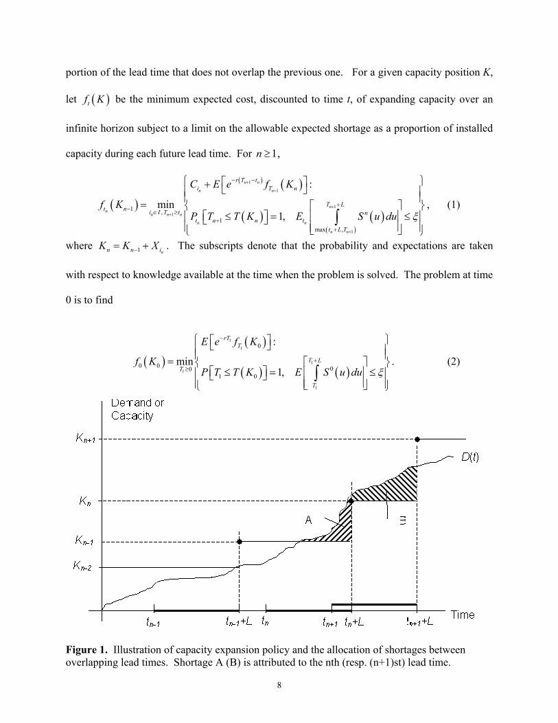
shortage is present only during lead times. Figure 1 illustrates shortages for a demand realization
with both non-overlapping and overlapping lead times. Let
( ) ( ){ } ( ){ }inf 0 : inf 0 :T x t D t x t P t x≡ ≥ = = ≥ = be the time at which demand first reaches the
level x. The automatic triggering of expansions can be expressed as a constraint that
( )1n nT T K −≤ with probability one for all n. For 1n nt L t t L++ ≤ < + , the shortage at time t as a
proportion of installed capacity is
( ) ( )max ,0nn nS t P t K K ≡ − .
At time 0, given 0K , the manager must choose a stopping time 1T at which the first expansion
will begin. From then on, at the realized time , 1nt n ≥ , the problem is: Given 1nK − and
knowledge of demand up to time nt , choose the capacity increment ni and the next expansion
epoch 1nT + to minimize the cost from time nt onward while controlling the expected shortage
during the lead time [ )1 1,n nT T L+ + + . However, lead times may overlap. To avoid double-
counting shortages, the choice of 1nT + is made to control the expected shortage only in the
8
portion of the lead time that does not overlap the previous one. For a given capacity position K,
let ( )tf K be the minimum expected cost, discounted to time t, of expanding capacity over an
infinite horizon subject to a limit on the allowable expected shortage as a proportion of installed
capacity during each future lead time. For 1n ≥ ,
( )
( ) ( )
( ) ( )( )
1
1
1
1
1
1 ,1
max ,
:
min1,
n n
n n
nn
n n n
n n
n n
r T ti T n
T Lt n i I T t n
t n n tt L T
C E e f K
f KP T T K E S u du ξ
+
+
+
+
+
− −
+− ∈ ≥
++
+ = ≤ = ≤
∫
, (1)
where 1 nn n iK K X−= + . The subscripts denote that the probability and expectations are taken
with respect to knowledge available at the time when the problem is solved. The problem at time
0 is to find
( )( )
( ) ( )
1
1
1
1
1
0
0 0 001 0
:
min1,
rTT
T LT
T
E e f K
f KP T T K E S u du ξ
−
+≥
= ≤ = ≤
∫
. (2)
Figure 1. Illustration of capacity expansion policy and the allocation of shortages between overlapping lead times. Shortage A (B) is attributed to the nth (resp. (n+1)st) lead time.
9
3. Timing and Choice of Expansions
The expansion policy must address both the timing and the sizes of expansions. Although these
policy aspects are obviously related, in this paper we show that for the formulation above, they
can be considered sequentially. The expansion times are found according to stopping rules that
compare demand with capacity position. Then, under this timing policy, the sequence of
facilities to install can be found by solving a deterministic problem without lead times.
3.1. Timing Policy Consider the timing decisions first. If L = 0, the manager could simply wait until demand equals
installed capacity and then, balancing economies of scale against the high present worth cost of a
large expansion, choose a quantity to install that would be instantaneously available. Despite the
uncertainty in demand, there would be no risk of capacity shortage. However, when L > 0, it is
possible that even though an expansion is undertaken when excess capacity remains, demand
will grow so fast during the lead time that shortages occur before the new capacity becomes
available. To derive the stopping times, we use the following result (Hull 2000):
Lemma 1: If V is a lognormal random variable and the standard deviation of lnV is s,
then ( ) ( ) ( ) ( )1 2max ,0E V K E V d K d − = Φ − Φ , where [ ]( )( )21 ln 2d E V K s s= + ,
2 1d d s= − and ( )Φ ⋅ is the standard normal cumulative distribution function.
Theorem 1 (Timing Policy): Let 0 < p < 1 be such that
( ) ( )2 2
0
ln 2 ln 2Lt
p t p tpe dt
t tγ
γ σ γ σξ
σ σ
+ + + − Φ − Φ =
∫ , (3)
and assume ( ) 00P pK< . For 1n ≥ , let ( )1n nT T pK+ = . Then the constraints on { }, 1nT n ≥ in
the formulation (1) and (2) will be satisfied.
10
Proof: That ( )1 1nt n nP T T K+ ≤ = for 0n ≥ where 0 0t ≡ , is satisfied trivially since p <
1 implies that ( ) ( )n nT pK T K≤ . For the expected shortage constraint in (1), note
that given ( )1nP t + at the realized time 1nt + , if 1nu t +≥ then ( )P u is lognormal
with mean ( ) ( )11
nu tnP t eγ +−
+ and the standard deviation of ( )ln P u is 1nu tσ +− .
Furthermore, the distribution of ( )1
1
n
n
T L n
TS u du+
+
+
∫ depends on events up to time 1nT +
only through ( )1nP T + and nK . Therefore, since ( ) 0nS u ≥ and the stopping time
1nT + is selected at time nt ,
( )( )
( ) ( ) ( )1 1 1
1
1 1 1
1max ,
n n n
n n n
n n n n
T L T L t Ln n n
t t t nt L T T t
E S u du E S u du E S u P t du+ + +
+
+ + +
+ + +
++
≤ =
∫ ∫ ∫ ,
regardless of the value of 1nt + . Let ( )( )( ) ( )( )2
1 11
1
ln 2n n nn
n
P t K u tu
u t
γ σδ
σ+ +
+
+ + −=
−
and ( ) ( )2 1 1n n
nu u u tδ δ σ += − − . Then
( ) ( ) ( ) ( ) ( )( ) ( )( )1 1
1
1 1
11 1 2
n n
n
n n
t L t Lu tnn n n
nnt t
P tE S u P t du e u u du
Kγ δ δ
+ +
+
+ +
+ +−+
+
= Φ − Φ
∫ ∫
by Lemma 1. Substitute ( )1n np P t K+= and 1nt u t += − for the result. The
requirement that 1n nT t+ ≥ for 1n ≥ holds since 1n nK K −> . The proof for the
expected shortage constraint in (2) is similar, and ( ) 00P pK< guarantees that
1 0T ≥ . ■
This timing policy is consistent with that followed in established service industries. For
example, electric power generation companies have traditionally maintained a reserve margin, R,

11
of capacity specified as a proportion of current demand (Kahn 1988). Assuming lead times do
not overlap, the need for the nth expansion would be indicated when ( )( )( ) ( )t P t P t RΚ − < .
Our policy compares demand to the capacity position ( ) 1nt K −Π = at time nt , and initiates an
expansion when the reserve margin drops to 1 1R p= − . Also, note that Lemma 1 can be used
to derive the Black-Scholes formula for the value of a European call option on an asset. Birge
(Birge 2000) has previously pointed out the correspondence between future excess demand and
this option value; namely, demand corresponds to asset price, capacity takes the place of strike
price, and the future time point in question is represented by the option’s expiration date. Having
insufficient capacity to meet the demand is analogous to selling one’s competitors an option to
capture the excess demand.
The ability to impose a stationary timing policy to satisfy the same shortage constraint in
every lead time relies on the Markovian character of the demand process and the assumption of
fixed lead times. For the geometric Brownian motion demand process, with shortage expressed
as a proportion of installed capacity, the Black-Scholes analysis suggests an appropriate form for
the timing policy. For other Markovian demand processes, e.g., different transformations of
Brownian motion, one might be able to identify the policy’s form but would have no analytical
means to specify the policy parameters (see Ryan (2003) for the use of simulation to specify a
timing policy for a different demand process). The fixed lead time assumption allows the
expansion timing and size decisions to be decoupled. If expansion lead time depends on
expansion size, one could follow a generalized form of the timing policy with ( )1n n nT T p K+ = ,
where the pair ( ),n ni p must be optimized jointly at time nt .
Note that an increasing sequence of capacity levels { }, 0nK n ≥ implies that { }, 1nT n ≥ is
a nondecreasing sequence of random variables. In order for the expansion policy to cover the
12
infinite horizon, it is necessary that nT → ∞ with probability one. If nK → ∞ , this condition is
guaranteed with probability 1 by the Hölder continuity of Brownian paths (Borodin and
Salminen 1996).
Lemma 2: The Brownian motion with drift is Hölder continuous of order α for any 0 1 2α< < ,
i.e., for all t > 0, 0 1 2α< < and almost all sample paths ω, there exists ( ),tc α ω such that for all
u, s < t,
( ) ( ) ( ),, , tB u B s c u s ααω ω ω− ≤ − .
Theorem 2: If ( )1n nT T pK+ = for 0n ≥ and nK → ∞ then nT → ∞ with probability 1.
Proof: For any sample path ω, the random variable ( )nT ω can be written as
( ) ( ) ( ) ( ){ }
( ) ( )( ) ( ){ }
,1
1
inf 0 : 0 ,0 0
inf 0 : , ln ln 0 ,0 0 .
B un n
n
T u P e pK B
u B u K P p B
ωω ω
ω ω
−
−
= ≥ = =
= ≥ = − =
Since ( ){ }nT ω is monotone increasing, it suffices to show that for any time t < ∞ , with
probability 1 there exists N such that ( )NT tω > .
Choose t < ∞ and 0 1 2α< < . Let ω be a Hölder continuous path of order α.
Suppose ( )mT tω ≤ for some 1m ≥ . Then by Lemma 2, for any ( )mT s tω < < ,
( )( ) ( ) ( ) ( )( ) ( ) ( )( ), ,, ,m t m t mB T B s c s T c t Tα α
α αω ω ω ω ω ω ω− ≤ − ≤ − .
Since nK → ∞ , there exists N such that ( )( )1 1 ,ln lnN m t mK K c t Tα
α ω− −− > − . Therefore,
( )NT tω > .■
13
3.2. Increment Policy Under the expansion timing policy, with parameter p determined according to the specified
allowable expected lead time shortage ξ, the remaining problem is to choose ni at time nt , 1n ≥ ,
such that nK → ∞ and the infinite horizon expected discounted cost is minimized. This problem
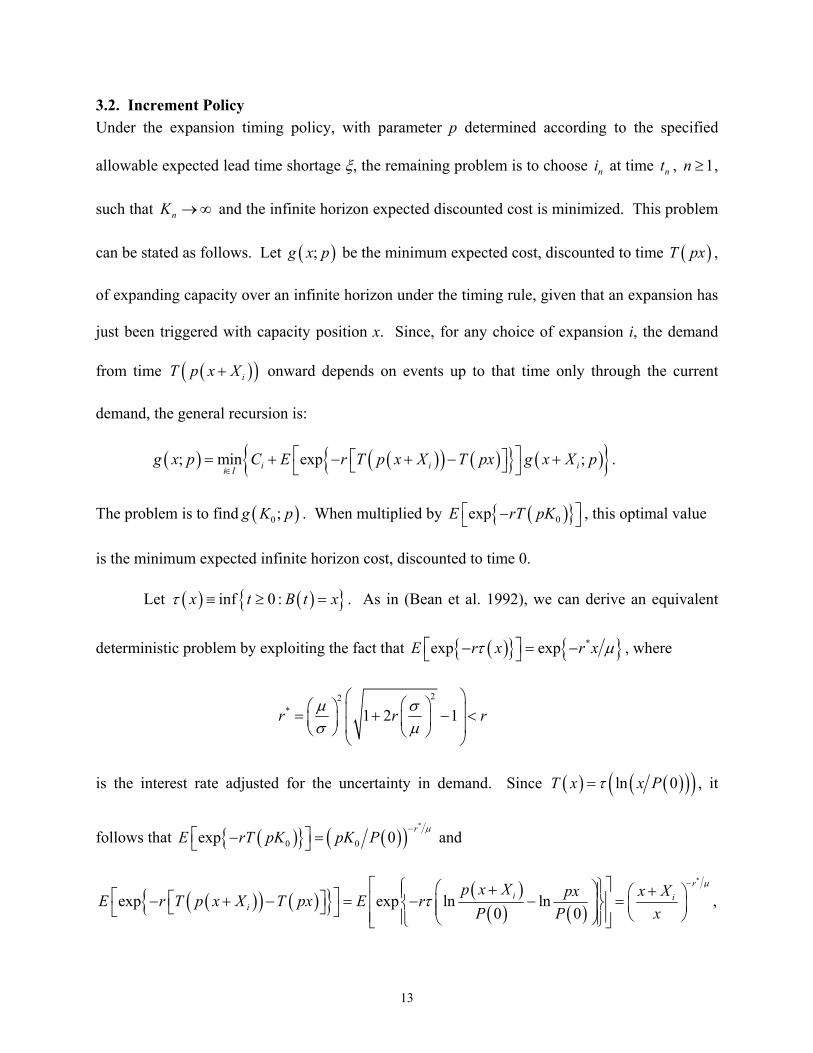
can be stated as follows. Let ( );g x p be the minimum expected cost, discounted to time ( )T px ,
of expanding capacity over an infinite horizon under the timing rule, given that an expansion has
just been triggered with capacity position x. Since, for any choice of expansion i, the demand
from time ( )( )iT p x X+ onward depends on events up to that time only through the current
demand, the general recursion is:
( ) ( )( ) ( ){ } ( ){ }; min exp ;i i ii Ig x p C E r T p x X T px g x X p
∈ = + − + − + .
The problem is to find ( )0;g K p . When multiplied by ( ){ }0expE rT pK − , this optimal value
is the minimum expected infinite horizon cost, discounted to time 0.
Let ( ) ( ){ }inf 0 :x t B t xτ ≡ ≥ = . As in (Bean et al. 1992), we can derive an equivalent
deterministic problem by exploiting the fact that ( ){ } { }*exp expE r x r xτ µ − = − , where
22
* 1 2 1r r rµ σσ µ
= + − <
is the interest rate adjusted for the uncertainty in demand. Since ( ) ( )( )( )ln 0T x x Pτ= , it
follows that ( ){ } ( )( )*
0 0exp 0r
E rT pK pK Pµ− − = and
( )( ) ( ){ } ( )( ) ( )
*
exp exp ln ln0 0
ri i
i
p x X x XpxE r T p x X T px E rP P x
µ
τ− + + − + − = − − =
,
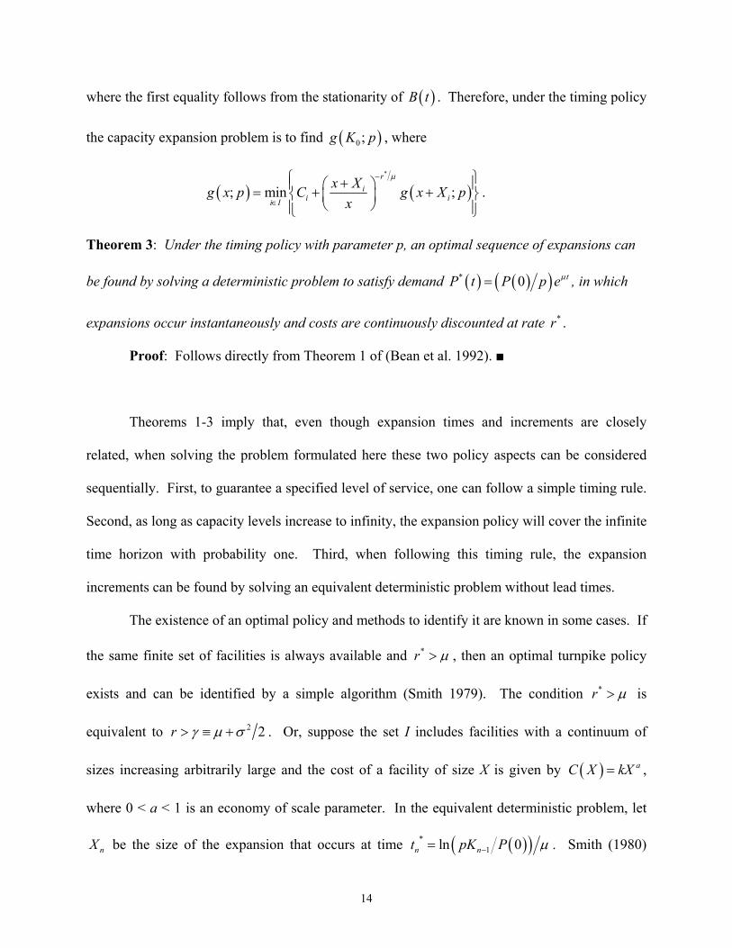
14
where the first equality follows from the stationarity of ( )B t . Therefore, under the timing policy
the capacity expansion problem is to find ( )0;g K p , where
( ) ( )*
; min ;r
ii ii I
x Xg x p C g x X px
µ−
∈
+ = + +
.
Theorem 3: Under the timing policy with parameter p, an optimal sequence of expansions can
be found by solving a deterministic problem to satisfy demand ( ) ( )( )* 0 tP t P p eµ= , in which
expansions occur instantaneously and costs are continuously discounted at rate *r .
Proof: Follows directly from Theorem 1 of (Bean et al. 1992). ■
Theorems 1-3 imply that, even though expansion times and increments are closely
related, when solving the problem formulated here these two policy aspects can be considered
sequentially. First, to guarantee a specified level of service, one can follow a simple timing rule.
Second, as long as capacity levels increase to infinity, the expansion policy will cover the infinite
time horizon with probability one. Third, when following this timing rule, the expansion
increments can be found by solving an equivalent deterministic problem without lead times.
The existence of an optimal policy and methods to identify it are known in some cases. If
the same finite set of facilities is always available and *r µ> , then an optimal turnpike policy
exists and can be identified by a simple algorithm (Smith 1979). The condition *r µ> is
equivalent to 2 2r γ µ σ> ≡ + . Or, suppose the set I includes facilities with a continuum of
sizes increasing arbitrarily large and the cost of a facility of size X is given by ( ) aC X kX= ,
where 0 < a < 1 is an economy of scale parameter. In the equivalent deterministic problem, let
nX be the size of the expansion that occurs at time ( )( )*1ln 0n nt pK P µ−= . Smith (1980)
15
showed that, if *r aµ> (equivalently, ( ) 2 2r a aµ σ> + ), then an optimal sequence of
expansion sizes is given by ( ) ( )1* * *0 1
n
nX K v v−
= − , where ** Tv eµ= , and
( )( )
( )*
0*
0
1arg min
1
aT
r a TT
k K eT
e
µ
µ− −>
−=
−.
Under this expansion size policy, the capacity levels increase geometrically as ( )* *0
n
nK K v=
and the size of the nth facility to install is a constant proportion * 1v − of the capacity position at
time nt . Even if *r aµ≤ so that discounted costs may diverge, there is a long run optimal policy
(Sinden 1960) that follows the same form.
The simplicity of the policy with constant p and v invites further exploration. Though the
form of the size policy depends on the form of the timing policy, the optimal value of v is
independent of the value of p that was chosen to control shortages. Finally, though we cannot
guarantee that lead times will not overlap, the expansion size controls the probability that they do
so.
Theorem 4: Suppose that ( ){ }1inf 0 :n nT t P t pK −= ≥ = , where 0 , 1nnK v K n= ≥ . Then for
1k ≥ , [ ]Pr n k nT T L+ < + is independent of n.
Proof: Conditioned on P(0), the first time P(t) reaches a value x, T(x) has density
( )( ) ( )( ) ( )( )( )2
23
ln 0ln 0;ln 0 , ln exp , 0
22
x P tx Pf t P x t
tt
µ
σσ π
− = − >
(Karlin and Taylor 1975). Therefore, using any realization tn as the origin, for 1k ≥ ,
( ) ( )21
0 230
lnlnPr exp22
Ln
n k n n
k v tk vT t L P t pv K dttt
µσσ π
−+
− > + = = − ∫ .■
16
In other words, the expansion policy is able to “keep up” with exponentially growing demand in
the sense that probability of lead times overlapping remains constant over the infinite horizon.
Finally, we note that Whitt (1981) assumed the use of the proportional expansion size
policy for geometric Brownian motion demand without lead times and under no particular
assumptions about expansion costs. Further, based on an empirical study of capacity utilization
in the chemical product industry, Lieberman (1989) identified this policy as the one most
commonly followed.
4. Policy Parameters
For the case where I is continuous with unbounded facility sizes and the cost of a facility of
size X is given by ( ) aC X kX= , given the form of the optimal policy specified in the condition
of Theorem 4, the problem remains to identify values for the policy parameters, or decision
variables, p and v. Clearly, the value of p that achieves a specified value for the allowable
expected shortage, ξ, depends on the demand parameters and the lead time length. The optimal
size factor, v, is independent of the lead time, but is affected by the demand parameters and the
cost economies of scale. In this section we seek a qualitative understanding of how the demand
parameters, µ and σ, affect both policy parameters as well as the magnitude of these effects
relative to those caused by the expansion parameters, a and L.
The value of p that achieves a specified expected shortage ratio, ξ, can be identified by
solving Equation (3) for p. Though no closed form solution is available, for practical purposes
one can plot or tabulate the value of ξ as a function of p, then invert the graph or table. Consider
baseline parameter values of µ = 0.05 (mean logarithmic growth rate of 5% per year), r = 0.1
(annual risk-adjusted interest rate used to discount costs), σ = 0.2 (standard deviation of
logarithmic demand growth), lead time L = 0.5 year, economy of scale parameter a = 0.9, with

17
cost constant k = 1. For this baseline case, the expected geometric growth rate of demand, γ, is
seven percent per year.
Figure 2 shows the values of p that achieve various values of expected shortage ratio, ξ,
and its sensitivity to doubling µ, σ2, or L (changing a single parameter at a time). Any of these
changes reduces p, provoking earlier expansions. However, doubling the variance of logarithmic
demand growth over a unit interval has a greater effect than doubling its mean.
0 0.005 0.01 0.015 0.02ξ
0.75
0.8
0.85
0.9
0.95
p
2L
è!!!!2σ2µ
Base
Figure 2. Value of the timing parameter (ratio of demand to capacity position) that achieves a specified expected shortage ratio.
The optimal capacity factor, v, can be found simply by minimizing
( ) ( ) ( )( )*
1 1a a rc v v v µ−= − − . For 1a < and *r µ> , one can verify that ( )c v′ has a unique root
*v ; ( )c v′ < 0 for v < *v and ( )c v′ > 0 for v > *v ; and ( )* 0c v′′ > . Therefore, *v is a unique
global minimizer. Figure 3 shows the value of the expansion timing parameter found for ξ =
0.001 paired with the optimal size parameter for the base case and for alterations in each
parameter singly. For ease of interpretation, the timing parameter expressed in terms of the
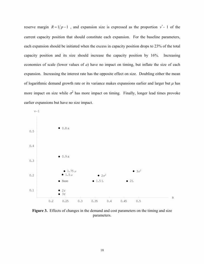
18
reserve margin 1 1R p= − , and expansion size is expressed as the proportion *v - 1 of the
current capacity position that should constitute each expansion. For the baseline parameters,
each expansion should be initiated when the excess in capacity position drops to 23% of the total
capacity position and its size should increase the capacity position by 16%. Increasing
economies of scale (lower values of a) have no impact on timing, but inflate the size of each
expansion. Increasing the interest rate has the opposite effect on size. Doubling either the mean
of logarithmic demand growth rate or its variance makes expansions earlier and larger but µ has
more impact on size while σ2 has more impact on timing. Finally, longer lead times provoke
earlier expansions but have no size impact.
0.2 0.25 0.3 0.35 0.4 0.45 0.5R
0.1
0.2
0.3
0.4
0.5
v−1
Base1.5µ 2σ2
2r3r
0.9a
1.75 µ 3σ2
0.8a
2L1.5L
Figure 3. Effects of changes in the demand and cost parameters on the timing and size parameters.
19
6. Conclusions
Many studies of capacity expansion have neglected lead times for adding capacity. In these
studies, it is safe to assume that shortages will never occur, and a regeneration point structure has
simplified the analysis. When lead times are included, the potential for capacity shortage cannot
be ignored; however, with uncertain demand these shortages are difficult to estimate. This paper
shows how a formula developed in the context of financial option pricing can be applied to
estimate the shortages that may result from a particular capacity expansion policy. We have
shown that a timing policy that maintains a constant expected lead time shortage (as a proportion
of installed capacity) provides a regeneration point structure that leads to an equivalent
deterministic formulation of the remaining problem to identify minimum cost expansion
increments. Policy parameters that minimize the cost of maintaining a specified service level
can be computed easily.
This paper’s contributions are (1) a justification and motivation of a timing policy that
has been commonly used by service providers who face significant expansion lead times; (2) a
proof, under this timing policy and for a particular cost assumption, of the optimality of an
expansion size policy that has been studied extensively without lead times and also observed in
practice; and (3) an exploration of how changes in the demand parameters, lead time length, and
economies of scale affect the combined use of the timing and expansion size policies. There are
two basic approaches to protecting against shortages that may result from the combination of
lead times and demand uncertainty: to begin installing capacity when significant excess capacity
remains, or to install large capacity increments. The numerical results in this paper indicate that,
while lead times influence timing and cost parameters determine expansion size, demand
characteristics affect both policy dimensions but in different ways. A high expected demand
growth motivates large expansions that occur somewhat earlier than otherwise. When demand
20
uncertainty is high, larger expansions are necessary but the main impact is to provoke earlier
installations.
An important extension of this research is to consider the impact of shortages in
economic terms rather than via a service level constraint. For facilities providing services to
dependent customers, the shortage cost functions are likely to be strictly convex. Computing
expected values of these costs to combine with expansion costs poses a significant challenge.
Acknowledgements: This work was supported by the National Science Foundation under grant
number DMI-9996373. An early version of this paper was published in the Proceedings of the
2000 Manufacturing and Service Operations Management Conference. I am grateful to Ananda
Weerasinghe for several helpful discussions.
References
Angelus, A., Porteus, E., and Wood, S. C. (2000). "Optimal sizing and timing of modular
capacity expansions." Report 1479R2, Graduate School of Business, Stanford University.
Angelus, A. and Porteus, E. (2003). "Using Echelon Capacity to Manage Multi-Resource
Capacity Expansions and Deferrals." Technical Report, Graduate School of Business,
Stanford University, Stanford, CA.
Bar-Ilan, A. and Strange, W. C. (1996). "Investment Lags." The American Economic Review,
86(3), 610-622.
Bean, J. C., Higle, J., and Smith, R. L. (1992). "Capacity expansion under stochastic demands."
Operations Research, 40, S210-S216.
Bean, J. C., and Smith, R. L. (1985). "Optimal capacity expansion over an infinite horizon."
Management Science, 31(12), 1523-1532.

21
Bieler, D., and Stevenson, I. (1998). "Internet Market Forecasts: Global Internet Growth 1998-
2005." Ovum Report, Ovum.
Birge, J. R. (2000). "Option methods for incorporating risk into linear planning models."
Manufacturing & Service Operations Management, 2(1), 19-31.
Borodin, A. N., and Salminen, P. (1996). Handbook of Brownian Motion: Facts and Formulae,
Birkhauser Verlag, Basel.
Çakanyıldırım, M. and Roundy, R. O. (2002). "Optimal capacity expansion and contraction
strategies under demand uncertainty." Technical Report, School of Management,
University of Texas at Dallas.
Chaouch, B. A., and Buzacott, J. A. (1994). "The effects of lead time on plant timing and size."
Production and Operations Management, 3(1), 38-54.
Davis, M. H. A., Dempster, M. A. H., Sethi, S. P., and Vermes, D. (1987). "Optimal capacity
expansion under uncertainty." Advances in Applied Probability, 19, 156-176.
Freidenfelds, J. (1981). Capacity Expansion: Analysis of Simple Models with Applications,
North-Holland, New York.
Hull, J. C. (2000). Options, Futures and Other Derivatives, Prentice Hall, Upper Saddle River,
NJ.
Kahn, E. (1988). Electric Utility Planning & Regulation, American Council for an Energy-
Efficient Economy, Washington, DC.
Karlin, S., and Taylor, H. M. (1975). A First Course in Stochastic Processes, Academic Press,
New York.
Lee, H. L., and Nahmias, S. (1993). "Single-product, single-location models." Handbooks in OR
& MS, 4, 3-55.
22
Lieberman, M. B. (1989). "Capacity utilization: theoretical models and empirical tests."
European Journal of Operational Research 40, 155-168.
Luenberger, D. G. (1998). Investment Science, Oxford University Press, New York.
Majd, S., and Pindyck, R. S. (1987). "Time to build, option value, and investment decisions."
Journal of Financial Economics, 18, 7-27.
McDonald, R., and Siegel, D. (1986). "The value of waiting to invest." Quarterly Journal of
Economics, 101, 707-727.
Min, K. J., and Wang, C.-H. (2002). "Discrete real options models for inter-related generation
projects." Proceedings of the 2002 Industrial Engineering Research Conference,
Orlando, FL.
Nickell, S. (1977). "Uncertainty and lags in the investment decisions of firms." Review of
Economic Studies, 44, 249-263.
Rai, A., Ravichandran, T., and Samaddar, S. (1998). "How to anticipate the Internet's global
diffusion." Communications of the ACM, 41(10), 97-106.
Ryan, S. M. (2003). "Capacity expansion with lead times and correlated random demand." Naval
Research Logistics 50(2), 167-183.
Sinden, F. X. (1960). "The replacement and expansion of durable equipment." Journal of the
Society of Industrial & Applied Mathematics, 8(3), 466-480.
Smith, R. L. (1979). "Turnpike results for single location capacity expansion." Management
Science, 25(5), 474-484.
Smith, R. L. (1980). "Optimal expansion policies for the deterministic capacity problem." The
Engineering Economist, 25(3), 149-160.
23
Srinivasan, T. N. (1967). "Geometric rate of growth of demand." Investments for Capacity
Expansion: Size, Location, and Time-Phasing, A. S. Manne, ed., MIT Press, Cambridge,
150-156.
Whitt, W. (1981). “The stationary distribution of a stochastic clearing process.” Operations
Research 29(2), 294-308.


