

CFD SIMULATION OF RISER VIV
A Dissertation
by
ZHIMING HUANG
Submitted to the Office of Graduate Studies of
Texas A&M University
in partial fulfillment of the requirements for the degree of
DOCTOR OF PHILOSOPHY
May 2011
Major Subject: Ocean Engineering
CFD Simulation of Riser VIV
Copyright 2011 Zhiming Huang
CFD SIMULATION OF RISER VIV
A Dissertation
by
ZHIMING HUANG
Submitted to the Office of Graduate Studies of
Texas A&M University
in partial fulfillment of the requirements for the degree of
DOCTOR OF PHILOSOPHY
Approved by:
Chair of Committee, Hamn-Ching Chen
Committee Members, Richard S. Mercier
Kuang-An Chang
Jean-Luc Guermond
Head of Department, John Niedzwecki
May 2011
Major Subject: Ocean Engineering

iii
ABSTRACT
CFD Simulation of Riser VIV. (May 2011)
Zhiming Huang, B.S., Tsinghua University; M.S., University of Houston
Chair of Advisory Committee: Dr. Hamn-Ching Chen
The dissertation presents a CFD approach for 3D simulation of long risers. Long
riser VIV simulation is at the frontier of the CFD research area due to its high demand
on computational resources and techniques. It also has broad practical application
potentials, especially in the oil and gas industry. In this dissertation, I used a time
domain simulation program - Finite-Analytic Navier-Stokes (FANS) code to achieve the
3D simulations of riser VIV.
First, I developed a riser modal motion solver and a direct integration solver to
calculate riser dynamic motions when subject to external forces. The direct integration
solver provides good flexibility on inclusion of riser bending stiffness and structural
damping coefficients. I also developed a static catenary riser solver based on trial and
error iteration technique, which allowed the motion solvers to handle catenary risers and
jumpers with arbitrary mass distribution. I then integrated the riser motion solvers to the
existing FANS code, and applied the CFD approach to a series of riser VIV problems
including a 2D fixed/vibrating riser, a 3D vertical riser in uniform and shear currents, a
3D horizontal riser in uniform and shear current, a hypothetic 3,000 ft marine top
tensioned riser in uniform current, a practical 1,100m flexible catenary riser in uniform
iv
current, and a hypothetic 265m flexible jumper partially submerged in uniform current. I
developed a VIV induced fatigue calculation module based on rain flow counting
technique and S-N curve method. I also developed a modal extraction module based on
the least squares method. The VIV details, including flow field vorticities, rms a/D, riser
motion trajectories, PSDs, modal components, VIV induced stress characteristics, and
VIV induced fatigue damages were studied and compared to the published experimental
data and results calculated using other commercial software tools. I concluded that the
CFD approach is valid for VIV simulations in 3D. I found that the long riser VIV
response shows complex behaviors, which suggests further investigation on the lock-in
phenomenon, high harmonics response, and sensitivity to the lateral deflections.

v
DEDICATION
The dissertation is dedicated to my wife Tracy Hou who has supported me all the
way since the beginning of this research work.
Also, this dissertation is dedicated to my daughter Chloe Huang who has been a
great source of inspiration.

vi
ACKNOWLEDGEMENTS
I would like to thank my committee chair, Dr. Chen, and my committee
members, Dr. Mercier, Dr. Chang, and Dr. Guermond, for their guidance and support
throughout the course of this research.
Thanks also go to my friends and colleagues and the department faculty and staff
for making my time at Texas A&M University a great experience. I also want to extend
my gratitude to the Department of Interior, Minerals Management Service (MMS),
Offshore Technology Research Center (OTRC), and American Bureau of Shipping
(ABS) for their kind funding of this research work.
Finally, thanks to my mother and father for their encouragement and to my wife
for her patience and love.

vii
NOMENCLATURE
2D 2-Dimension
3D 3-Dimension
a VIV Response Amplitude
iα Modal Component Corresponding to the ith Mode
Ca Added Mass Coefficient
Cd Drag Coefficient
CF Cross-Flow
CFD Computational Fluid Dynamics
CL Lift Coefficient
D Riser Diameter
Do Pipe Outer Diameter
Ds Riser Structural Damping Coefficient
E Riser Pipe Young’s Modulus
fz0 The Mean Zero-Up-Crossing Frequency
h Riser Mesh Length
I Riser Sectional Moment of Inertia
IL In-Line
0ξ Initial Error for Numerical Scheme Stability Check
iξ Riser Modal Shape Function Corresponding to the ith Mode
L Riser Overall Length

viii
m Riser Unit Mass
N Riser Mesh Total Element Number
PSD Power Spectral Density
ρ Fluid Density
rms Root-Mean-Square
Re Reynolds Number
θ Riser Declination Angle
τ Simulation Time Step
T Riser Effective Tension
U Current Velocity
U1 Current Velocity at Riser 1st End
U2 Current Velocity at Riser 2nd End
Umax Maximum Current Velocity
VIV Vortex Induced Vibration

ix
TABLE OF CONTENTS
Page
ABSTRACT.............................................................................................................. iii
DEDICATION .......................................................................................................... v
ACKNOWLEDGEMENTS ...................................................................................... vi
NOMENCLATURE.................................................................................................. vii
TABLE OF CONTENTS .......................................................................................... ix
LIST OF FIGURES................................................................................................... xii
LIST OF TABLES .................................................................................................... xx
CHAPTER
I INTRODUCTION AND LITERATURE REVIEW............................ 1
II VIV SIMULATION TECHNIQUES................................................... 8
Numerical Approach ...................................................................... 8
Riser Motion Modal Solver............................................................ 12
Riser Motion Direct Integration Solver.......................................... 14
Numerical Scheme Stability Check................................................ 16
Motion Solver Static Case Validation ............................................ 19
Motion Solver Dynamic Case Validation ...................................... 21
VIV Induced Fatigue Calculation .................................................. 23
Stress Histogram Characteristics.................................................... 24
S-N Curve Approach ...................................................................... 27
Partially Submerged Catenary Jumper Static Configuration ......... 29
VIV Response Modal Extraction ................................................... 35
Jumper Transient Response............................................................ 39
Integration of Motion Solver to Parallel Fluid Solver.................... 42
x
CHAPTER Page
III 2D SIMULATION OF FLOW PAST
A FIXED/VIBRATION RISER........................................................... 46
Data Grid ........................................................................................ 47
Riser Interference Analysis Procedures ......................................... 49
Simulation Results.......................................................................... 50
Riser Clearance Check Results ...................................................... 58
Discussions..................................................................................... 60
IV 3D SIMULATION OF FLOW PAST
A VERTICAL RISER IN UNIFORM CURRENT.............................. 61
Data Grid ........................................................................................ 62
Simulation Results.......................................................................... 65
Discussions..................................................................................... 81
V 3D SIMULATION OF FLOW PAST
A VERTICAL RISER IN SHEAR CURRENT................................... 83
Simulation Results.......................................................................... 84
Discussions..................................................................................... 95
VI 3D SIMULATION OF FLOW PAST
A HORIZONTAL RISER IN UNIFORM CURRENT........................ 97
Simulation Results.......................................................................... 101
Discussions..................................................................................... 117
VII 3D SIMULATION OF FLOW PAST
A HORIZONTAL RISER IN SHEAR CURRENT............................. 118
Simulation Results.......................................................................... 119
Discussions..................................................................................... 135
VIII 3D SIMULATION OF FLOW PAST
A 3000FT RISER IN UNIFORM CURRENT..................................... 136
Simulation Results.......................................................................... 139
Discussions..................................................................................... 147

xi
CHAPTER Page
IX 3D SIMULATION OF FLOW PAST
A CATENARY RISER IN UNIFORM CURRENT............................ 148
Simulation Results.......................................................................... 157
Discussions..................................................................................... 164
X 3D SIMULATION OF FLOW PAST A PARTIALLY
SUBMERGED JUMPER IN UNIFORM CURRENT......................... 166
Simulation Results.......................................................................... 170
Discussions..................................................................................... 179
XI SUMMARY AND CONCLUSIONS................................................... 181
REFERENCES.......................................................................................................... 187
APPENDIX A ........................................................................................................... 195
VITA ......................................................................................................................... 198
xii
LIST OF FIGURES
Page
Figure 1 CFD Simulation Procedures...................................................................... 11
Figure 2 von Neumann Stability Check (EI Sensitivity) ......................................... 18
Figure 3 von Neumann Stability Check (Damping Sensitivity) .............................. 18
Figure 4 Riser Static Displacement Comparison (Riser Constant Tension)............ 19
Figure 5 Riser Static Displacement Comparison (Varying Tension) ...................... 20
Figure 6 Riser Dynamic Motion Comparison (Time History at x/L=1/3)............... 21
Figure 7 Riser Dynamic Motion Comparison (Forced Vibration) .......................... 22
Figure 8 Distinct Stress Cycle Number Calculation ................................................. 26
Figure 9 Stress Range Histograms ........................................................................... 26
Figure 10 Stress Combination Sketch ....................................................................... 28
Figure 11 Jumper General Arrangement ................................................................... 30
Figure 12 Jumper Element Free Body Diagram........................................................ 32
Figure 13 Jumper Static Configuration ..................................................................... 33
Figure 14 Jumper Effective Tension Distribution..................................................... 34
Figure 15 Modal Amplitude Comparison ................................................................. 38
Figure 16 Jumper Deformation under Impulse Load ................................................ 40
Figure 17 Jumper Response Distribution .................................................................. 41
Figure 18 Overset Grid for Wake Field Computation............................................... 48

xiii
Page
Figure 19 Overset Grid for Wake Field Computation – Riser Surface Vicinity....... 49
Figure 20 Riser Interference Analysis Flow Chart.................................................... 50
Figure 21 Vorticity Contours for Fixed Riser ........................................................... 52
Figure 22 Wake Field 3D View – Top:Huse’s Formula, Bottom:CFD .................... 53
Figure 23 Wake Field Contour – Top:Huse’s Formula, Bottom:CFD...................... 54
Figure 24 Effective Drag Coefficient ........................................................................ 55
Figure 25 Vorticity Contours for Vibrating Riser ..................................................... 56
Figure 26 Wake Field behind a Vibrating Riser ....................................................... 57
Figure 27 Effective Drag Coefficient on Vibrating Riser ......................................... 58
Figure 28 Riser Displacement along Riser – Huse’s Formula .................................. 59
Figure 29 Riser Displacement along Riser – FANS ................................................. 59
Figure 30 Data Grids at x/L=Constant ...................................................................... 63
Figure 31 Grid Details on Riser Surface and Overlapping Region........................... 63
Figure 32 Data Grids with Riser Deflection.............................................................. 64
Figure 33 Vortex Shedding Evolution, Left: U=0.42 m/s, Right: U=0.84 m/s......... 69
Figure 34 Vortex Contour, Top: U=0.42 m/s, Bottom: U=0.84 m/s......................... 70
Figure 35 Riser Deflection Time History, x/L=0.5 ................................................... 71
Figure 36 Riser CF Response (U=0.42 m/s) ............................................................. 71
Figure 37 Riser CF Response (U=0.84 m/s) ............................................................. 72
xiv
Page
Figure 38 Cross Flow VIV RMS a/D, U=0.42 m/s................................................... 73
Figure 39 Cross Flow VIV RMS a/D, U=0.84 m/s................................................... 73
Figure 40 Riser Motion Trajectory Comparison (CFD)............................................ 74
Figure 41 Riser Motion Trajectory Comparison (Experimental Data) ..................... 75
Figure 42 Lift Coefficient (U=0.42 m/s, x/L=0.3) .................................................... 77
Figure 43 Lift Coefficient (U=0.42 m/s, x/L=0.5) .................................................... 78
Figure 44 Lift Coefficient (U=0.84 m/s, x/L=0.3) .................................................... 78
Figure 45 Lift Coefficient (U=0.84 m/s, x/L=0.5) .................................................... 79
Figure 46 CF Motion PSD (Experiment 1105) ......................................................... 79
Figure 47 CF Motion PSD (FANS, U=0.42 m/s)...................................................... 80
Figure 48 CF Motion PSD (Experiment 1108, U=0.84 m/s) .................................... 80
Figure 49 CF Motion PSD (FANS, U=0.84 m/s)...................................................... 81
Figure 50 Inclined Riser and Equivalent Shear Current ............................................. 83
Figure 51 Riser VIV Evolution, Left: U2=0.42m/s, Right: U2=0.84m/s..................... 86
Figure 52 Riser VIV Snapshots, U2=0.42m/s ............................................................ 87
Figure 53 Riser VIV Snapshots, U2=0.84m/s ............................................................ 88
Figure 54 Riser Cross Flow Response Time History (U2=0.42m/s)........................... 89
Figure 55 Riser Cross Flow Response Time History (U2=0.84m/s)........................... 89
Figure 56 Riser Cross Flow Response rms a/D (U2=0.42m/s) ................................... 90
xv
Page
Figure 57 Riser Cross Flow Response rms a/D (U2=0.84m/s) ................................... 90
Figure 58 Riser Cross Flow Response PSD (Test 1205, U2=0.42m/s) ....................... 91
Figure 59 Riser Cross Flow Response PSD (CFD, U2=0.42m/s)............................... 91
Figure 60 Riser Cross Flow Response PSD (Test 1210, U2=0.84m/s) ....................... 92
Figure 61 Riser Cross Flow Response PSD (CFD, U2=0.84m/s)............................... 92
Figure 62 CF Fatigue Damage Index Comparison (U2=0.42m/s) ............................. 94
Figure 63 CF Fatigue Damage Index Comparison (U2=0.84m/s) ............................. 94
Figure 64 Riser VIV Testing Plan View Schematics ................................................ 97
Figure 65 Data Grids in 3D, Left: Undeformed Riser, Right: Deformed Riser ........ 100
Figure 66 Data Grid Near Riser Surface ................................................................... 100
Figure 67 Riser VIV Evolution, Left: U=0.4m/s, Right: U=0.8m/s.......................... 102
Figure 68 Riser VIV Snap Shots (U=0.4m/s) ........................................................... 104
Figure 69 Riser VIV Snap Shots (U=0.8m/s) ........................................................... 105
Figure 70 In-Line Modal Response (U=0.4m/s) ....................................................... 106
Figure 71 In-Line Modal Response (U=0.8m/s) ....................................................... 106
Figure 72 Mean Drag Coefficients............................................................................ 108
Figure 73 RMS of Lift Coefficients .......................................................................... 108
Figure 74 Riser Motion Trajectory, Left: U=0.4m/s, Right:U=0.8m/s ..................... 109
Figure 75 Riser Motion Trajectory at x/L=0.25, U=0.4m/s ...................................... 110

xvi
Page
Figure 76 Riser Motion Trajectory at x/L=0.35, U=0.4m/s ...................................... 110
Figure 77 Riser Motion Trajectory at x/L=0.55, U=0.4m/s ...................................... 110
Figure 78 Riser CF Response Envelope for U=0.4m/s, t=193~200.......................... 112
Figure 79 Riser CF Response Envelope for U=0.8m/s, t=193~200.......................... 113
Figure 80 Riser In Line VIV RMS for U=0.4m/s ..................................................... 113
Figure 81 Riser Cross Flow VIV RMS for U=0.4m/s............................................... 114
Figure 82 Riser In Line VIV RMS for U=0.8m/s ..................................................... 114
Figure 83 Riser Cross Flow VIV RMS for U=0.8m/s............................................... 115
Figure 84 Riser Cross Flow VIV Max RMS............................................................. 115
Figure 85 Riser Motions at x/L=0.25 and 0.75 ......................................................... 116
Figure 86 Linearly Shear Currents ............................................................................ 119
Figure 87 Vortex Shedding, Umax=0.4m/s, Left: Shear, Right: Uniform................ 122
Figure 88 Riser VIV Snap Shots, Left: Umax=0.4m/s, Right: Umax=0.8m/s.......... 123
Figure 89 Vorticity Contours, Left: Umax=0.4m/s, Right: Umax=0.8m/s ............... 123
Figure 90 Drag Coefficient Distribution, Umax=0.4m/s .......................................... 125
Figure 91 Lift Coefficient Distribution, Umax=0.4m/s ............................................ 125
Figure 92 Drag Coefficient Distribution, Umax=0.8m/s .......................................... 126
Figure 93 Lift Coefficient Distribution, Umax=0.8m/s ............................................ 126
Figure 94 Cross Flow VIV RMS a/D, Umax=0.4m/s ............................................... 128
xvii
Page
Figure 95 Cross Flow VIV RMS a/D, Umax=0.8m/s ............................................... 128
Figure 96 Cross Flow VIV Max RMS a/D ............................................................... 129
Figure 97 Riser Motion Trajectory, Umax=0.4m/s, Left: Shear, Right: Uniform .... 130
Figure 98 Riser Motion Trajectory, Umax=0.8m/s, Left: Shear, Right: Uniform .... 131
Figure 99 In-Line VIV Modal Response Amplitude ................................................ 133
Figure 100 Cross Flow VIV Modal Response Amplitude ........................................ 133
Figure 101 In-Line VIV Modal Response Energy .................................................... 134
Figure 102 Cross Flow VIV Modal Response Energy.............................................. 134
Figure 103 Riser Modal Shapes ................................................................................ 138
Figure 104 Riser VIV Comparison, Umax=0.4m/s, Left:Uniform, Right:Shear...... 141
Figure 105 Riser VIV Snapshot, Shear Current ........................................................ 142
Figure 106 Riser VIV Snapshot, Uniform Current ................................................... 143
Figure 107 Riser Cross Flow VIV Modal Response................................................. 144
Figure 108 Riser Cross Flow VIV rms a/D - Uniform Current ................................ 145
Figure 109 Riser Cross Flow VIV rms a/D - Shear Current ..................................... 145
Figure 110 Riser Cross Flow VIV Induced Stress – Uniform Current ..................... 146
Figure 111 Riser Cross Flow VIV Induced Stress – Shear Current.......................... 147
Figure 112 Flexible Flowline Curve Laying Schematic ........................................... 150
Figure 113 Data Grid along the Flexible Riser ......................................................... 154

xviii
Page
Figure 114 Flexible Catenary Riser Fundamental Modal Shapes............................. 156
Figure 115 Flexible Catenary Riser VIV Evolution Illustration (Top View) ........... 158
Figure 116 Cross Flow VIV rms a/D, U=0.7knot ..................................................... 159
Figure 117 Flexible Flowline Maximum Deflection, U=0.7knot ............................. 161
Figure 118 Drag Coefficient Distribution, U=0.7knot.............................................. 163
Figure 119 Jumper General Arrangement ................................................................. 167
Figure 120 Data Grid along the Flexible Jumper...................................................... 170
Figure 121 Jumper VIV Snapshot, Time Step=20,000 ............................................. 171
Figure 122 Jumper Mean Deflection due to Current Drag Force.............................. 172
Figure 123 Jumper VIV Vortex Shedding Pattern, s/L=0.25.................................... 174
Figure 124 Jumper VIV Vortex Shedding Pattern, s/L=0.5...................................... 175
Figure 125 Cross Flow VIV rms a/D ........................................................................ 176
Figure 126 Jumper Motion Modal Decomposition ................................................... 177
Figure 127 Jumper Motion Trajectory ...................................................................... 178
Figure 128 Drag Coefficient Time History Comparison .......................................... 195
Figure 129 Lift Coefficient Time History Comparison ............................................ 195
Figure 130 Motion Y Time History Comparison...................................................... 196
Figure 131 Motion Z Time History Comparison ...................................................... 196

xix
Page
Figure 132 Normalized Computational Time ........................................................... 197
Figure 133 Cross Flow rms a/D comparison............................................................. 197
xx
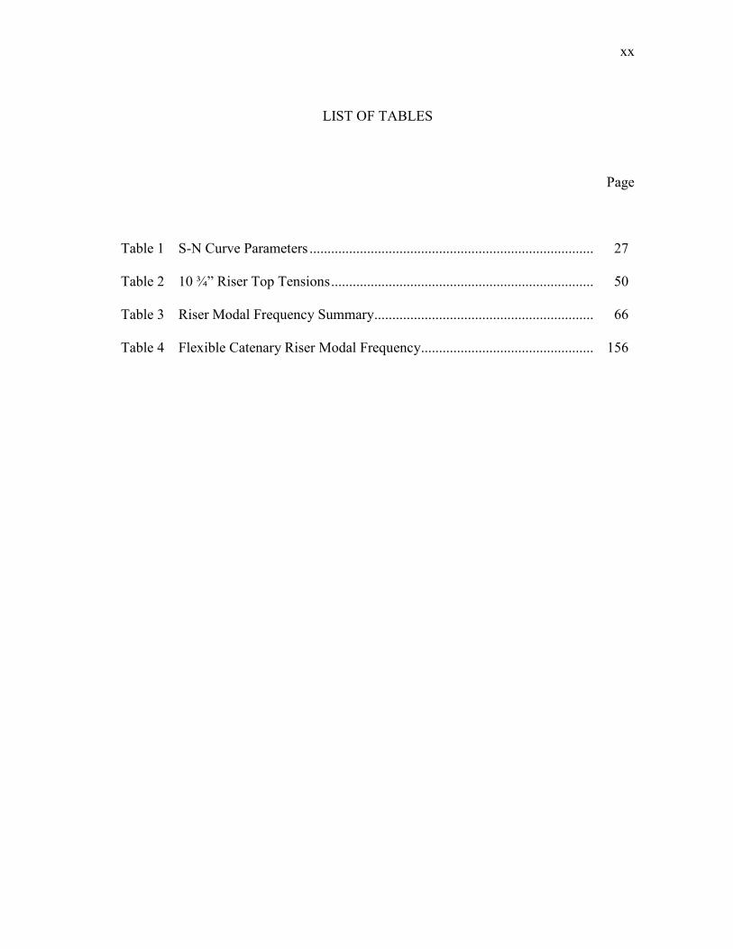
LIST OF TABLES
Page
Table 1 S-N Curve Parameters ............................................................................... 27
Table 2 10 ¾” Riser Top Tensions......................................................................... 50
Table 3 Riser Modal Frequency Summary............................................................. 66
Table 4 Flexible Catenary Riser Modal Frequency................................................ 156

1
CHAPTER I
INTRODUCTION AND LITERATURE REVIEW
Deepwater oil and gas exploration and developments have been moving fast
toward increasingly deeper water depth, i.e. 3,000m in Gulf of Mexico. Majority of the
subsea wells are tied back to a surface platform through long risers, including steel
catenary risers, flexible risers, free standing risers, bundled risers, or top tensioned risers
(ASME B31.4, 2002, ASME B31.8a, 2001, API 1111, 1999). These risers provide fluid
conduit for fluid transport between subsea wells and surface platform, and protect the
environment from reservoir fluid exposure. Many offshore facilities are designed for a
service life up to 30 years, including the riser systems. For riser system fatigue design,
one of the challenging areas is the VIV induced fatigue excited by ocean current flow.
Usually riser VIV is in high frequency range (~1Hz) comparing to the wave induced
dynamics (~0.1Hz). And it is one of the main sources of fatigue damage for the marine
riser design. Although the VIV could be suppressed by strakes or fairings, the cost
associated with the hardware and installation is high. Therefore, the research interest on
the riser VIV has been growing in the oil and gas industry to achieve safe and
economical design.
____________
This dissertation follows the style of Journal of Offshore Mechanics and Arctic
Engineering.
2
The oil and gas industry has been heavily relying on the experimental data for
riser VIV design. During the last several years many VIV experiments have been carried
out on deepwater risers with large L/D, and the related publications are numerous. The
Norwegian Deepwater Program measured on a 38 m (L/D=1,400) long riser model for
various linearly shear and uniform flow velocity cases corresponding to bare and straked
riser configurations, and the experimental results are discussed in Trim et al. (2005).
British Petroleum measured the VIV of a drilling riser under different riser conditions,
such as drilling, hung-off rig move, and connected non-drilling. The experiments were
conducted in the Gulf of Mexico in various water depths from 1,182 ft (L/D=300) to
6,800 ft (L/D=1,700) (Tognarelli et al. 2008). Deepstar JIP also carried out VIV
experiments in Gulf Stream in 2006. The experiments were done on a 500 ft long and
1.43 in. diameter (L/D=4,200) pipe with and without strakes. Part of the experimental
results was discussed by Vandiver et al. (2006) and Jhingran et al. (2008). In April of
2008, selected results of the above VIV experiments were released to the public and
hosted on web site oe.mit.edu/VIV/, along with some data sets donated by several others,
including two sets donated by ExxonMobil measured on a 10 m riser model with and
without strakes, and for various linearly shear and uniform flow velocity cases.
However, experiment has limitations as well, such as facility availability and
capacity limits, model scale limit, difficulty of current profile generation, cost concerns,
etc. Under such condition, software and computer models have been developed to meet
this need. Some software tools were developed based on experimental data and empirical
formula. These tools used model superposition approach, and the modal responses were

3
partially or fully based on the test data. Other tools were based on CFD simulation
approach. Some of the popular tools for riser VIV prediction were discussed by Chaplin
et al. (2005).
As a trend in recent years, the CFD approach received more and more attention
due to the ever-improving computational capability, i.e. computer speed and storage
space. Furthermore, the CFD approach also provides flow field and riser motion details
that are essential to understand the VIV phenomena, and is regarded as a valuable
compensation and good alternative to water basin experiments.
The application of the 3D CFD approach to cylinder VIV study is still a
relatively new research area due to its onerous computational requirement. Some early
work can be traced back to 1996. Newman and Karniadakis (1996) presented a 3D CFD
simulation of flexible cable VIV with aspect ratio (L/D) of 45, and low Reynolds
number (~300). Lucor et al. (2000) presented simulation results of a flexible cable with
aspect ratio of 500, and Reynolds number of 103. Willden & Graham et al. (2001) also
published the simulation results of VIV simulation of a flexible cylinder with aspect
ratio of 100, and Reynolds number of 300. Yamamoto et al (2004) simulated the VIV of
a 120 m marine riser with aspect ratio of 500, and Reynolds number 2x10⁵. Meneghini et
al. (2004) used two-dimensional discrete vortex method (DVM) to simulate long marine
risers with L/D up to 4,600. Pontaza, Chen & Chen (2006, 2007a, 2007b) presented
simulations of riser VIV with aspect ratio of 20, and Reynolds number up to 107. Holmes
& Oakley et al. (2006) simulated VIV of a long riser with aspect ratio of 1,400, and
Reynolds number of 104. They used unstructured data grid consisting of 10 million finite

4
elements. Constantinides and Oakley (2008a, 2008b) also presented the VIV simulations
of long cylinders with L/D=4,200. The prospect of increasing need for CFD simulation
has also attracted some commercial FEA software vendors. Chen and Kim (2010)
presented simulation results obtained through ANSYS MFX package, a newly released
feature by the ANSYS Inc. And Chen et al. studied the VIV of a vertical riser with
aspect ratio of 500, and Reynolds number of 104. In summary, the available publications
showed the latest research on CFD simulation of long riser VIV is mainly in three areas:
1. Quasi-3D or strip theory. In this approach the CFD simulation is down
graded to 2D strips, and the fluid field on each strip is independent of each
other. The advantage is that the data grids are in 2D and compatible with
many existing turbulence models. The vortex shedding in 2D planes could be
simulated in good resolution with relatively less elements. The disadvantage
is the fluid fields on different plane are not coupled, and riser spanwise
vorticity has been ignored.
2. Full 3D with unstructured data grid. In this approach the fluid field is
discretised by 3D elements. The advantage is that the fluid field is solved in
3D and riser spanwise flow could be captured in detail. The disadvantage is
that it requires significantly more elements near the riser surface to achieve
good resolution for turbulence model. Consequently the computational effort
could be tremendous even with the fastest computer to date. When riser has
large deflection, the data grid could be highly distorted to accommodate the
relative riser movement. This would compromise its validity for large riser

5
deflection situations, which are fairly common in the physical world,
especially in deepwater applications.
3. Full 3D with structured data grid. First, it is a full 3D approach. The flow
field around the riser is calculated by numerically solving the unsteady,
incompressible 3D Reynolds-Averaged Navier-Stokes (RANS) in
conjunction with a large eddy simulation (LES) model (Pontaza et al. 2004,
2005a, 2005b, 2005c). The governing equations are transformed from
physical space (x,y,z) into numerical space ( ξ,η,γ ). The continuity equation
is then solved by a finite-volume scheme. The transport equations are solved
by the finite-analytic method of Chen et al. (1990) assuming the pressure
field is known. The pressure is then updated by a hybrid PISO/SIMPLER
algorithm (Chen & Patel, 1988, 1989). Second, it uses structured data grid,
which possesses all advantages of the strip theory. Particularly, the Chimera
technique could be applied to allow for data grid overset. The Chimera
technique is well suited for CFD involving moving objects such as risers. A
very fine data grid (body grid) is attached to the riser and on top of a
relatively coarse grid (wake or background grid). When riser moves, the body
grid moves relative to the background grid. The data consistency between the
body grid and the background grid on the overlapped region is enforced by
data interpolation. Theoretically the data grids can be overlapped and nested
as many levels as possible. In some of our studies we added an intermediate
data grid (wake grid) to resolve the vortex shedding and traveling. By using
6
the Chimera technique, the data grids can be generated with great attention to
the details, such as the regions near the riser surface and vortex shedding and
traveling area, yet without worrying about the re-generation of data grid at
each time step when the riser moves.
The objective of this dissertation is to further develop the 3rd approach (FANS
code), and extend the capability of the existing code from 2D and 3D with short L/D to
3D with large L/D, with Reynolds number up to 1.5x10⁵. The research scope of work
includes the following tasks:
1. Development of CFD capabilities: riser motion modal solver.
2. Development of CFD capabilities: riser motion direct integration solver.
3. Development of fatigue calculation capabilities: riser VIV induced fatigue
calculation module.
4. Development of a riser catenary static solver for arbitrary weight distribution
using a trial and error method.
5. Development of a riser modal extraction module using the least squares
method.
6. 2D simulations of flow past a fixed riser at high Reynolds numbers
(Re=3x10⁵).
7. 2D simulations of flow past a forced motion riser at high Reynolds numbers
(Re=3x10⁵).
8. 3D simulations of flow past a vertically positioned riser in uniform current
(L/D=480, Re=1.5x10⁴).

7
9. 3D simulations of flow past a vertically positioned riser in shear current
(L/D=480, Re=1.5x10⁴).
10. 3D simulations of flow past a horizontally positioned riser in uniform current
(L/D=1,400, Re=1.7x10⁴).
11. 3D simulations of flow past a horizontally positioned riser in shear current
(L/D=1,400, Re=1.7x10⁴).
12. 3D simulations of flow past a vertically positioned riser in uniform current
(L/D=3,350, Re=8x10⁴).
13. 3D simulations of flow past a catenary riser in uniform current (L/D=3,300,
Re=1.1x10⁵).
14. 3D simulations of flow past a catenary, partially submerged jumper in
uniform current (L/D=800, Re=1.5x10⁵).
The simulation results were compared to the published experimental data, and/or
the results calculated using other commercial software tools.

8
CHAPTER II
VIV SIMULATION TECHNIQUES
This Chapter describes the numerical approach used for the riser VIV
simulations, and additional techniques developed throughout the research and case
studies.
Numerical Approach
The numerical approach we adopted is a time domain simulation code - Finite-
Analytic Navier-Stokes (FANS) code. It has been previously validated through various
applications (Pontaza, Chen & Chen, 2004, 2005a, 2005b; Pontaza, Chen & Reddy,
2005; Pontaza & Chen 2006) on 2D riser VIV simulations and 3D rigid riser VIV
simulations. The flow field around a riser is calculated by numerically solving the
unsteady, incompressible Navier-Stokes equations. The turbulent flow was solved using
Large Eddy Simulation (LES):
( )21 iji i
i j
j i j j i
u p uu u
t x x x x x
τν
ρ
∂∂ ∂ ∂ ∂+ = − + −
∂ ∂ ∂ ∂ ∂ ∂ , (1)
where the subgrid stresses are given by
ij i j i ju u u uτ = − ,
with the Smagorinsky subgrid-scale turbulence model:
2ij T ijSτ ν= − ,
( ) ijijST SSC 22Δ=ν ,

9
The local strain rate tensor ijS is defined as
∂
∂+
∂
∂=
i
j
j
iij
x
u
x
uS
2
1 ,
and the filter-width is taken as the local grid size, i.e.
( ) 3/1
zyx ΔΔΔ=Δ .
The Smagorinsky coefficient SC is chosen as 0.1. No damping is included in this model.
Refer to Chen et al. (2006) for more details.
The formulation is fully 3D without omitting any terms in the Navier-Stokes
equations. Therefore, it is not the same as 2D strip theory, which assumes that the flow is
purely two-dimensional without spanwise correlation. To limit the computational effort,
we used relatively coarse grids in spanwise direction. As a result, the flow in the
spanwise direction is “under-resolved”. The effect of the spanwise velocity correlations
has been studied in Pontaza and Chen (2006) on a short cylinder with sufficiently fine
mesh in the spanwise direction. Nevertheless, we were able to predict the riser motion
responses with reasonable accuracy and will leave the further improvement in spanwise
grid resolution to future investigations.
The overset grid (Chimera) technique is used to handle the riser movement and
grid overlapping. We adopted fine meshes on the riser cross-sectional planes and coarse
meshes in the riser spanwise direction. This would reduce the total element number and
the computational effort. The coordinate system is selected as (unless otherwise noted in
the content): x direction coincides with riser axis, y is in the flow direction, and z is the
cross flow direction. The data grid system consists of three sets (or two sets when the

10
background grid is not used) of data grids and has a total of less than 1.5 million grid
nodes. The three sets of data grids are: (1) body grid – the data grid adjacent to the riser
surface that provides fine resolution to calculate the fluid-riser surface interaction and
vortex generation, (2) wake grid – it interfaces with body grid and background grid and
provides good resolution for vortex propagation, (3) background grid – as the name
suggests, it defines the outer boundary of the computational fluid domain, provides the
far field fluid boundary conditions, interfaces with and provides a physical extension to
the wake grid using relatively coarse mesh. The data grid sizes are different for each
simulation, and more details are presented in the simulation result sections. When the
riser vibrates, the data grids also move with the riser so there is no gap between the riser
and the grids at any time.
The riser has various length and diameter, depending on the load case definitions.
During the simulations, the drag (Cd) and lift (CL) coefficients are calculated along the
riser at each time step. The riser is descritized using fine segments (usually 250 to 500
segments – a typical range for riser global dynamic analysis). Its two ends are pinned to
the ground with zero rotational stiffness. Then the riser motions are solved by a motion
solver (either the modal solver or the direct integration solver) assuming that the drag
and lift force variation is negligible at each time step. This is an explicit approach
without iteration between the flow field and the riser motion. When the VIV response
dominant modes are not very high (~ 1Hz), the riser bending stiffness should not impact
the VIV response. However, the riser direct integration motion solver allows for

11
inclusion of the bending stiffness, and structural damping as well. Fig. 1 shows the time
domain simulation procedures.
Generate Data Grids
Initialize Flow Field
Solve for u,v,w and p
Calculate Cd and CL
along Riser
Compute Riser
Displacements
Move Body Grids
Regenerate Data Grid
Interpolation Coefficients
t>tend
End
Begin
Yes
No
Fig. 1 CFD Simulation Procedures
12
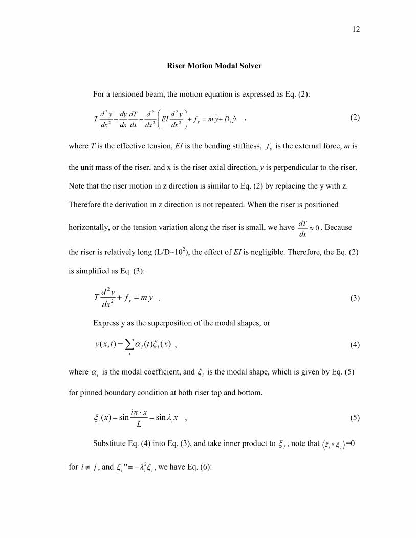
Riser Motion Modal Solver
For a tensioned beam, the motion equation is expressed as Eq. (2):
yDymfdx
ydEI
dx
d
dx
dT
dx
dy
dx
ydT sy
&+=+
−+
..
2
2
2
2
2
2
, (2)
where T is the effective tension, EI is the bending stiffness, yf is the external force, m is
the unit mass of the riser, and x is the riser axial direction, y is perpendicular to the riser.
Note that the riser motion in z direction is similar to Eq. (2) by replacing the y with z.
Therefore the derivation in z direction is not repeated. When the riser is positioned
horizontally, or the tension variation along the riser is small, we have 0≈dx
dT. Because
the riser is relatively long (L/D~102), the effect of EI is negligible. Therefore, the Eq. (2)
is simplified as Eq. (3):
..
2
2
ymfdx
ydT y =+ . (3)
Express y as the superposition of the modal shapes, or
∑=i
ii xttxy )()(),( ξα , (4)
where iα is the modal coefficient, and iξ is the modal shape, which is given by Eq. (5)
for pinned boundary condition at both riser top and bottom.
xL
xix ii λ
πξ sinsin)( =
⋅= , (5)
Substitute Eq. (4) into Eq. (3), and take inner product to jξ , note that ji ξξ ∗ =0
for ji ≠ , and iii ξλξ 2'' −= , we have Eq. (6):

13
2
2''
j
jy
jjj
fTm
ξ
ξαλα
∗=+ , (6)
where m is the modal mass, 2
jTλ is the modal stiffness, and RHS is the modal excitation
force. The natural periods are 2
2
mL
Tj
m
T j
j πλ
ω == , which is the standard solution of a
taut string.
Once we have yf at each time step, the modal coefficient jα could be solved
using Eq. (6). The lateral displacement ),( txy is then calculated through modal
superposition. Note that the RHS of the Eq. (6) will be integrated in y and z direction
separately to give modal excitation forces in the in-line and cross flow directions. Hence
Eq. (6) is solved in both y and z directions individually for the modal responses in in-line
and cross flow directions. No artificial or structural damping is included, although they
can be included by adding a damping term to Eq. (2) and following the same procedures
to derive the equivalent form of Eq. (6).
We used the 4th order Runge-Kutta method to integrate equation (5). This scheme
is explicit and stable for small time step integrations (Ti
mLt
πτ
2
2
≤=Δ ).
14
Riser Motion Direct Integration Solver
The tensioned beam equation can also be solved through a finite difference
scheme with direct integration at each time step. Notice that Eq. (2) is a parabolic system
of PDEs, with fourth order derivative in space and second order derivative in time. We
select the finite difference scheme of each term in Eq. (2) as:
2
11
2
2 2
h
yyy
dx
ydn
j
n
j
n
j −+ +−= , for j=2..N-1, and
2
12
2
2 2
h
yyy
dx
ydn
j
n
j
n
j +−= ++
, for j=1,
2
21
2
2 2
h
yyy
dx
ydn
j
n
j
n
j −− +−= , for j=N, (7)
h
yy
dx
dyn
j
n
j
2
11 −+ −= , for j=2..N-1, and
h
yyy
dx
dyn
j
n
j
n
j
2
43 21 ++ −+−= , for j=1
h
yyy
dx
dyn
j
n
j
n
j
2
34 12 +−= −−
, for j=N, (8)
4
2112
4
4 464
h
yyyyy
dx
ydn
j
n
j
n
j
n
j
n
j −−++ +−+−= , for j=3..N-2,
4
1123
4
4 464
h
xxxxx
dz
xdn
j
n
j
n
j
n
j
n
j −+++ +−+−= , for j=2,
4
1123
4
4 464
h
yyyyy
dx
ydn
j
n
j
n
j
n
j
n
j +−−− +−+−= , for j=N-1,
4
1234
4
4 464
h
yyyyy
dx
ydn
j
n
j
n
j
n
j
n
j +−+−= ++++
, for j=1,
4
1234
4
4 464
h
yyyyy
dx
ydn
j
n
j
n
j
n
j
n
j +−+−= −−−−
, for j=N, (9)

15
2
21
2
2 2
τ
−− +−=
n
j
n
j
n
j yyy
dt
yd, for n>=3, (10)
τ
1−−=
n
j
n
j yy
dt
dy, for n>=2, (11)
Initial conditions are set as 021 == jj yy , j=1..N. Assume EI is constant, dx
dTw = ,
and assemble Eqs (7) to (11), we have the discretized governing Eq. (12)
n
j
n
j
n
j
jj
n
j
sjn
j
jjn
j
RHSyh
EIy
h
EI
h
w
h
T
yDm
h
EI
h
Ty
h
EI
h
w
h
Ty
h
EI
=+
++−
++++
+−−
++
−−
24142
24214224
4
2
624
2 ττ, (12)
where 2
2
1
2
2 −− −
++= n
j
n
j
sn
jx
n
j ym
yDm
fRHSτττ
, h is the riser segment length, and τ is the
time step. Note that this is an implicit scheme. Its matrix dimension is N x N, and can be
solved by LU decomposition method. The same discretization scheme is also used to
solve for the riser cross flow motion in z-direction.
At each time step, the pressure and viscous force on the riser surface are integrated
circumferentially and mapped to the riser structural elements. The riser in-line and cross
flow motions are then calculated and fed back to the body grid as boundary conditions.
The riser is typically discretized into 250 to 500 structural elements. If the riser has
constant sectional properties then the element sizes will be uniform through out the riser
string. It is worth noting that this method is a linearized motion solver with consideration
that the riser VIV is usually in the order of several diameters. The riser motions are solved
in in-line and cross flow directions separately.
16
Numerical Scheme Stability Check
The stability of the numerical scheme is checked through von Neumann method.
The stability check considers only the finite difference solution of the structural response,
and does not include the fluid structure interaction. With an initial error vector 0ξ , the
error distribution at time step n and node j is expressed as ( ) jinn
j eG θξ = , where yk Δ= πθ .
Substitute it to Eq. (13), we have
( ) ( ) ( )
( ) ( ) ( ) ( ) ,24
2
624
2
2
2
1
2
)2(
4
)1(
42
242
)1(
42
)2(
4
jinjinsjinjinjj
jinsjjinjjjin
eGm
eGDm
eGh
EIeG
h
EI
h
w
h
T
eGDm
h
EI
h
TeG
h
EI
h
w
h
TeG
h
EI
θθθθ
θθθ
τττ
ττ
−−++
−−
−
+=+
++−
++++
+−−
(13)
Dividing both sides of Eq. (13) by jineGm ⋅θ
τ 2, and let
)sin(22
162
)cos(24
)2cos(2
2
4
2
2
2
4
2
2
2
4
2
θττττ
θττ
θτ
−
++++
+−=
mh
wi
m
D
mh
EI
mh
T
mh
EI
mh
T
mh
EIA
jsjj ,
+−=m
DB sτ2 ,
1=C ,
Eq. (13) is simplified as 0** 2 =++ CGBGA , and the amplification factor G is
given by:
A
ACBBG
2
42
2,1
−±−= .
17
For the special case of 0=sD and 0=w (i.e., Tj = const), the present numerical
scheme is unconditionally stable with 11
12,1 <
++=
βαG , where
2sin
16 4
4
2 θτα
mh
EI=
and 2
sin4 2
2
2 θτβ
mh
T= . The inclusion of damping term
m
Dsτδ = usually improves the
numerical stability. It can be shown analytically that 1)1(2
)(4)2(1
2
2,1 ≤+++
+−±+=≤−
δβαβαδδ
G
for all combinations of α, β and δ as given below:
≥+−≤+++
+≤≤
+++≤
<+−<+++
=
0)(4,11
1
1
10
0)(4,11
1
2
2,1
2
2,1
βαδδβα
δδβα
βαδδβα
ifG
ifG
.
Therefore, Eq. (13) is unconditionally stable. For illustration purpose, a typical
0.273 m (10.75 in) production riser for 900 m (3,000 ft) water depth is used for the von
Neumann stability check. It has uniform mass of 180 kg/m (121 lb/ft), mean tension of
500 kN. It is discretized by 250 elements and with simulation time step τ=0.007 s. Fig. 2
shows the von Neumann stability under different bending to tension ratios. The higher the
bending stiffness, the better the stability. Fig. 3 shows the von Neumann stability under
different damping coefficients. In this case the bending was set to zero (EI=0). It indicates
that the damping has limited effect on the stability of the numerical scheme.
A riser motion solver is then established based on this numerical difference
scheme to predict the riser dynamic motions during VIV simulations.

18
von Neumann Stability Check (EI Sensitivity)
0
0.2
0.4
0.6
0.8
1
0 90 180 270 360
θθθθ
| G |
EI/TL2=1x10-3
EI/TL2=1x10-4
EI/TL2=1x10-2
EI/TL2=0
Fig. 2 von Neumann Stability Check (EI Sensitivity)
von Neumann Stability Check (EI/TL2=0, Damping Sensitivity)
0.8
0.85
0.9
0.95
1
1.05
0 90 180 270 360
θθθθ
| G |
µµµµ=Ds/2/(mT/L)1/2
µ=10-3
µ=10-2
µ=10-1
µ=0
µ=0.5
µ=0.2
Fig. 3 von Neumann Stability Check (Damping Sensitivity)

19
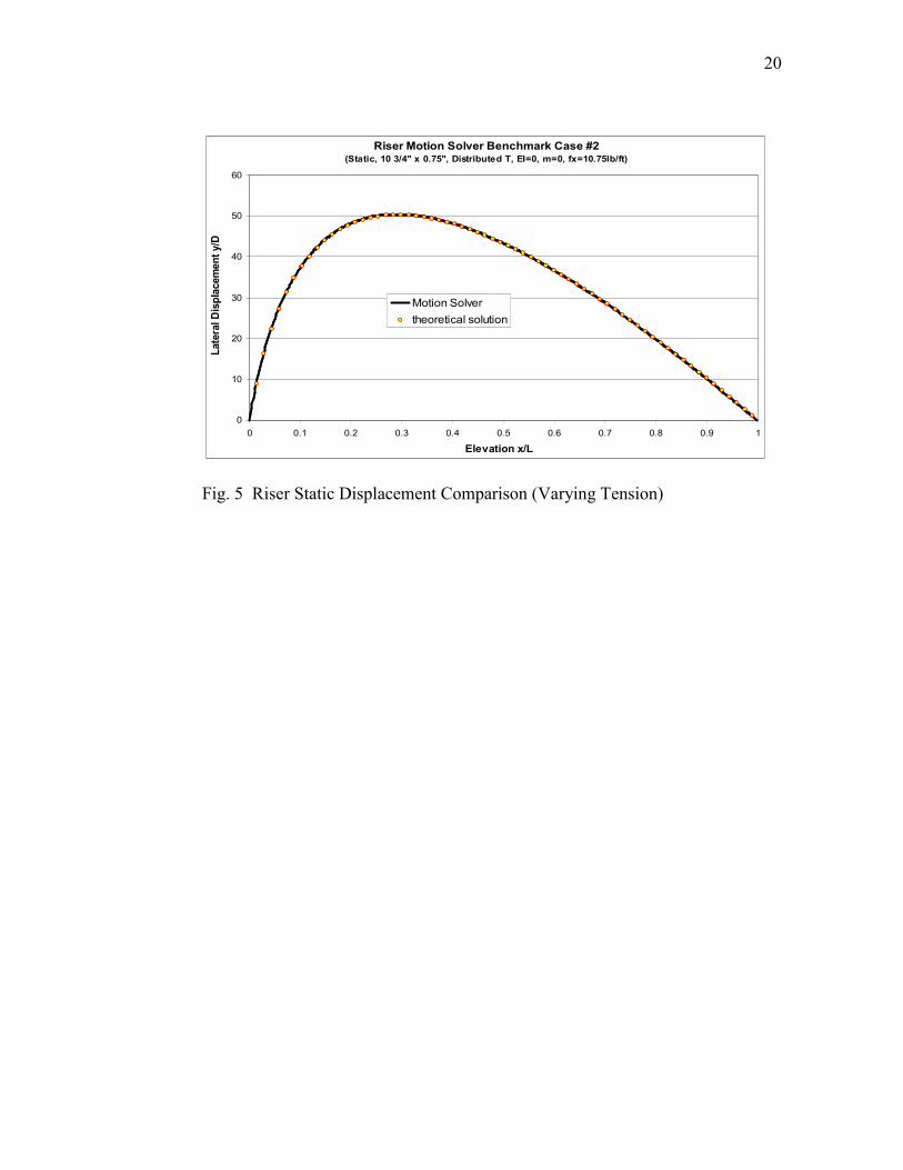
Motion Solver Static Case Validation
The riser motion solver is applied to solve for the riser deflection under constant
loads. Two cases were checked against the theoretical solution: (1) a 0.273 m (10.75 in)
riser with constant tension, (2) a 0.273 m (10.75 in) riser with linearly varying tension
distribution. In the reality the top tensioned risers have the highest tension at the top, and
lowest tension at the bottom due to its own submerged weight. The results are shown in
Figs. 4 and 5 for these two cases respectively. For the constant tension case, the riser
deflection is symmetric and the maximum riser deflection occurs in the middle of the
riser string. However, for the varying tension case, the riser deflection is not symmetric
and the maximum riser deflection occurs in the lower portion of the riser. The
comparisons in both cases show exact match between motion solver and theoretical
solution.
Riser Motion Solver Benchmark Case #1(Static, 10 3/4" x 0.75", EI=0, m=0, fx=10.75lb/ft)
0
5
10
15
20
25
30
35
0 0.1 0.2 0.3 0.4 0.5 0.6 0.7 0.8 0.9 1
Elevation x/L
Lateral Displacement y/D (ft)
Motion Solver
theoretical solution
Fig. 4 Riser Static Displacement Comparison (Riser Constant Tension)
20
Riser Motion Solver Benchmark Case #2(Static, 10 3/4" x 0.75", Distributed T, EI=0, m=0, fx=10.75lb/ft)
0
10
20
30
40
50
60
0 0.1 0.2 0.3 0.4 0.5 0.6 0.7 0.8 0.9 1
Elevation x/L
Lateral Displacement y/D
Motion Solver
theoretical solution
Fig. 5 Riser Static Displacement Comparison (Varying Tension)

21
Motion Solver Dynamic Case Validation
When the riser is suddenly subject to a uniform load, it will start to move and
vibrate until its energy dissipates completely. Fig. 6 shows the vibrating time history at
location x/L=1/3, where the maximum riser deflection occurs. Typical structural
damping coefficient of 0.3% was included. Solutions of dynamic response from the
finite difference method were compared to those from a commercial finite element code
(Flexcom) to test this aspect of the finite difference method. And the comparison also
confirms that the riser motion solver with the proposed difference schemes is able to
predict riser dynamic motions correctly.
Riser Motion Solver Benchmark Case - Step Load( x/L=1/3, 10 3/4" x 0.75", Distributed T, m>0, fx=10.75lb/ft )
0
10
20
30
40
50
60
70
80
90
100
0 10 20 30 40 50 60
time (sec)
Lateral Displacement y/D
Motion Solver
FEA tool
Fig. 6 Riser Dynamic Motion Comparison (Time History at x/L=1/3)

22
A forced vibration case was also used to check the riser motion solver. A
sinusoidal motion with amplitude of two diameters and period of one second is applied
to the riser top, and the riser lateral deflection time histories have been recorded and
plotted. Again, these riser deflections are compared to a FEA tool, as shown in Fig. 7. It
shows the riser dynamic motions are very similar.
Riser Motion Solver Benchmark - Forced Vibration( 10 3/4" x 0.75", Distributed T, Xtop=2*sin(2ππππ *t) )
-10
-7.5
-5
-2.5
0
2.5
5
7.5
10
0 0.2 0.4 0.6 0.8 1
x/L
y/D
riser motion envelope by FEA tool
riser motion envelope by Motion Solver
Fig. 7 Riser Dynamic Motion Comparison (Forced Vibration)
.

23
VIV Induced Fatigue Calculation
Riser VIV could cause large quantity of fatigue stress cycles. Although the stress
includes tension induced stress from riser length variation and bending induced stress
from curvature variation, usually bending induced stress is dominant. For long risers, the
VIV induced bending stress at the outer diameter can be calculated as
),(2
),( '' txyED
tx o=σ , where E is the Young’s modulus, Do is the outer diameter of the
riser. Therefore, the Eq (14) can be derived:
∑=i
iioED
tx ''2
),( ξασ , (14)
where 2
),()(
j
j
j
txyt
ξ
ξα
∗= .
There are many different ways to calculate fatigue. We adopted rain flow counting
in conjunction with S-N curve approach since it is popularly used and regarded as the most
accurate method. The procedures are as follows:
1. Simulate riser VIV in time domain for sufficiently long duration.
2. Calculate the curvatures at each time step for all the riser elevations.
3. Generate riser stress time histories at riser locations of interest.
4. Count the stress cycles using Rain Flow Counting techniques.
5. Accumulate the fatigue damage through Palmgren-Miner’s rule and S-N
curve approach.
In step 3 the stress time histories are dependent of the circumferential angle if both
the in-line and cross flow VIV induced fatigue are to be considered. We calculate the in-

24
line and cross flow stresses first and then combine them at the riser outer diameter. An
alternative method is to calculate the riser 3D curvature in step 2.
Stress Histogram Characteristics
Once the riser dynamic motions are known, the bending stress responses can be
calculated from the riser curvatures. Tension stress variation is neglected since it is usually
much lower than the bending stress variations. For a steady VIV response, the stress time
history can be expressed as a series of sinusoidal components with modal frequencies:
∑∞
=
+⋅=1
)sin()(i
ii tibt ϕωσ , (15)
where ω is the riser fundamental frequency, ib and iϕ are the response amplitude and
phase angle of mode i respectively.
Let’s assume mode n is the most dominant mode, and rearrange Eq. (15) as:
∑∞
=
+⋅−+⋅=1
))(sin()(i
ii tnitnbt ϕωωσ . (16)
Note that
))sin(()cos(
))cos(()sin())(sin(
i
ii
tnitn
tnitntnitn
ϕωω
ϕωωϕωω
+⋅−⋅+
+⋅−⋅=+⋅−+⋅ . (17)
Substitute Eq. (17) into Eq. (16), we have
∑∑∞
=
∞
=
+⋅−⋅++⋅−⋅=11
))sin(()cos())cos(()sin()(i
ii
i
ii tnibtntnibtnt ϕωωϕωωσ . (18)
During stress cycle counting, only stress peaks and troughs are needed. At the
stress peaks and troughs, the stress derivatives with respect to time must be zeroes, or:
25
0)(
=dt
tdσ. (19)
Take derivative of both sides in Eq. (18), we have:
∑∑∞
=
∞
=
+⋅−⋅⋅−+⋅−⋅⋅=11
))sin(()sin())cos(()cos()(
i
ii
i
ii tnibitntnibitndt
tdϕωωωϕωωω
σ . (20)
Combine Eqs. (19) and (20), Eq. (21) is derived finally:
∑
∑∞
=
∞
=
+⋅−⋅
+⋅−⋅=⋅
1
1
))sin((
))cos((
)tan(
i
ii
i
ii
tnibi
tnibi
tn
ϕωω
ϕωωω . (21)
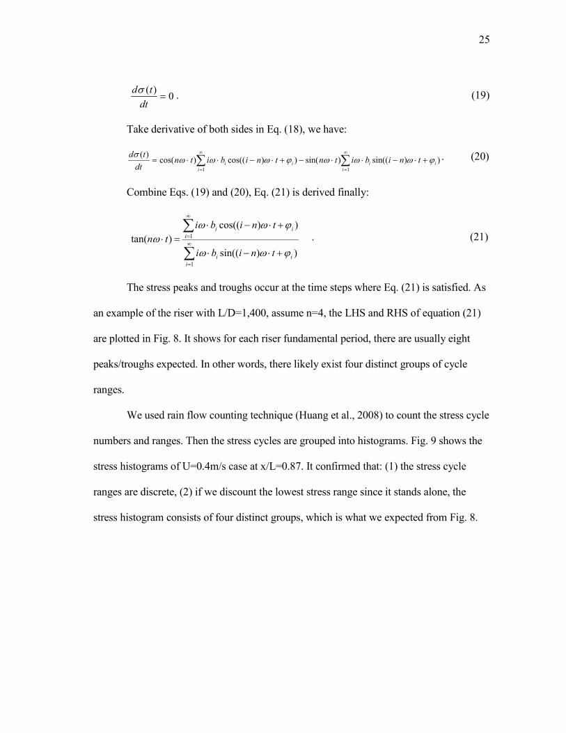
The stress peaks and troughs occur at the time steps where Eq. (21) is satisfied. As
an example of the riser with L/D=1,400, assume n=4, the LHS and RHS of equation (21)
are plotted in Fig. 8. It shows for each riser fundamental period, there are usually eight
peaks/troughs expected. In other words, there likely exist four distinct groups of cycle
ranges.
We used rain flow counting technique (Huang et al., 2008) to count the stress cycle
numbers and ranges. Then the stress cycles are grouped into histograms. Fig. 9 shows the
stress histograms of U=0.4m/s case at x/L=0.87. It confirmed that: (1) the stress cycle
ranges are discrete, (2) if we discount the lowest stress range since it stands alone, the
stress histogram consists of four distinct groups, which is what we expected from Fig. 8.

26
Stress Response Peak/Trough Number Graph (n=4)
-10
-8
-6
-4
-2
0
2
4
6
8
10
0 0.125 0.25 0.375 0.5 0.625 0.75 0.875 1
t/To
LHS(t), RHS(t)
LHS(t)
RHS(t)
Fig. 8 Distinct Stress Cycle Number Calculation
Stress Range Histogram (U=0.4m/s)
0.0E+00
3.0E+06
6.0E+06
9.0E+06
1.2E+07
1.5E+07
0 0.5 1 1.5 2 2.5
Stress (ksi)
Cycle Number
x/L=0.87
Fig. 9 Stress Range Histograms
27
S-N Curve Approach
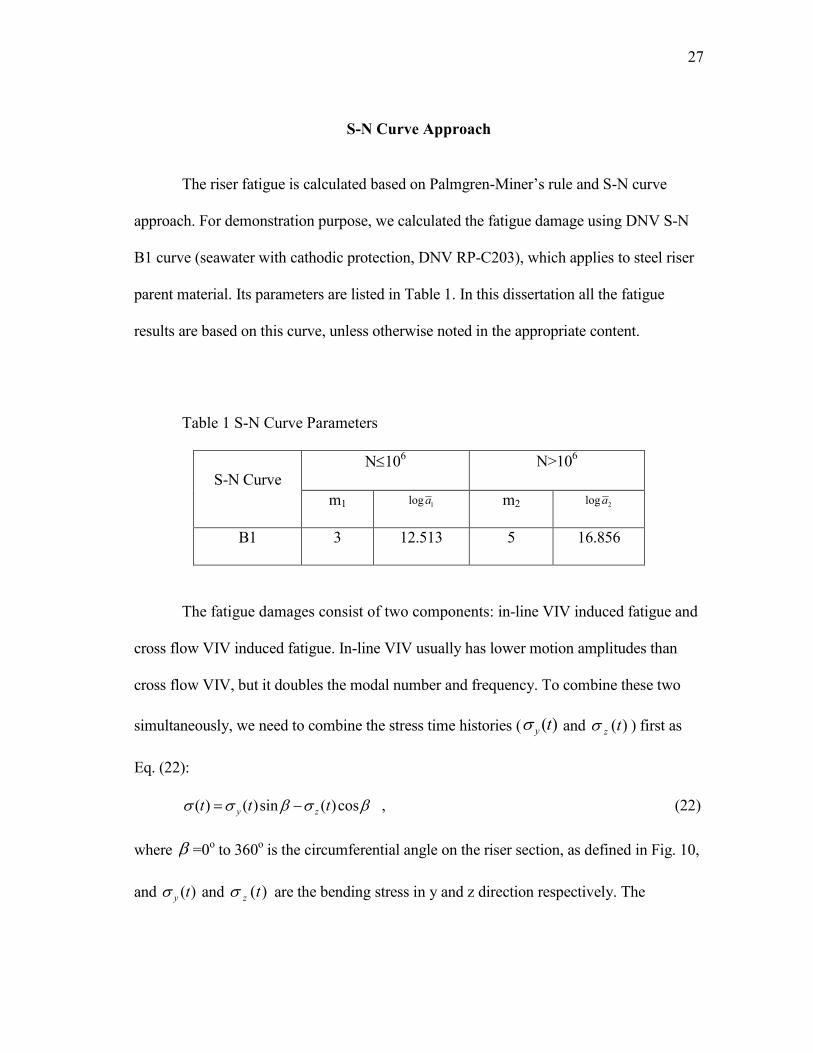
The riser fatigue is calculated based on Palmgren-Miner’s rule and S-N curve
approach. For demonstration purpose, we calculated the fatigue damage using DNV S-N
B1 curve (seawater with cathodic protection, DNV RP-C203), which applies to steel riser
parent material. Its parameters are listed in Table 1. In this dissertation all the fatigue
results are based on this curve, unless otherwise noted in the appropriate content.
Table 1 S-N Curve Parameters
N≤106 N>106
S-N Curve
m1 1loga m2 2loga
B1 3 12.513 5 16.856
The fatigue damages consist of two components: in-line VIV induced fatigue and
cross flow VIV induced fatigue. In-line VIV usually has lower motion amplitudes than
cross flow VIV, but it doubles the modal number and frequency. To combine these two
simultaneously, we need to combine the stress time histories ( )(tyσ and )(tzσ ) first as
Eq. (22):
βσβσσ cos)(sin)()( ttt zy −= , (22)
where β =0o to 360
o is the circumferential angle on the riser section, as defined in Fig. 10,
and )(tyσ and )(tzσ are the bending stress in y and z direction respectively. The

28
combined stress time histories are then processed for stress histograms and fatigue
damages. Both of them are functions of β and x/L.
Y
Z
ββββ
βσβσσ cos)(sin)()( ttt zy −=
Fig. 10 Stress Combination Sketch
The fatigue calculation requires only the output results from the VIV simulations,
and it can be performed after the simulations are completed. Therefore, it was designed as
a stand-alone module that reads in the simulation results, and processes the curvatures and
fatigue distributions along the riser.
The fatigue damage index (DI) (Tognarelli et al., 2004) is a parameter
approximately proportional to the fatigue damage. For S-N curves with single slope
m1=3, the expression is as 3
0 zz rmsfDI = , where the zrms is the standard deviation of
the bending strain time histories, which is related to the bending stress (Eq. 22) through
Young’s modulus E. And 0zf is the mean zero-up-crossing frequency for the stress
response.
29
Partially Submerged Catenary Jumper Static Configuration
Flexible jumpers are special risers with relatively short length and low bending
stiffness. The flexible jumpers are widely used in oil and gas industry to transport liquid
or gas content between two facility units, usually located close to each other and have
relative movement. In many of its applications, the jumper is positioned near the water
surface, sometimes surface piecing, hence subject to severe environmental loads,
including strong surface currents. To study a flexible jumper VIV, its catenary shape
needs to be determined first.
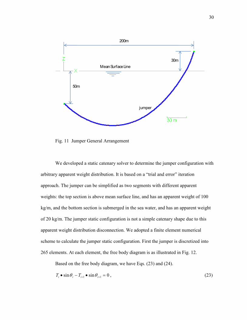
Fig. 11 shows a typical jumper arrangement. In this hypothetical case the
jumper’s first end is attached to a submerged facility at 50 m below the mean surface
level, and its second end is attached to a hang-off porch at 30 m above the mean surface
level. The nominal horizontal span is 200 m. The jumper has a diameter of 0.33 m, and
total length is 265 m (L/D=800). Its air weight is 100 kg/m, and submerged weight 20
kg/m (mass ratio=1.0). The mass ratio is 2/ Dm ρ (Vandiver, 1993). A uniform current of
0.5 m/s (1 knot) is applied in the direction perpendicular to the jumper catenary plane.
The upper section (about 10% of overall length) of the jumper is in the air, and the lower
section (about 90% of the overall length) is submerged in the water.
30
200m
50m
30m
MeanSurface Line
jumper
Fig. 11 Jumper General Arrangement
We developed a static catenary solver to determine the jumper configuration with
arbitrary apparent weight distribution. It is based on a “trial and error” iteration
approach. The jumper can be simplified as two segments with different apparent
weights: the top section is above mean surface line, and has an apparent weight of 100
kg/m, and the bottom section is submerged in the sea water, and has an apparent weight
of 20 kg/m. The jumper static configuration is not a simple catenary shape due to this
apparent weight distribution disconnection. We adopted a finite element numerical
scheme to calculate the jumper static configuration. First the jumper is discretized into
265 elements. At each element, the free body diagram is as illustrated in Fig. 12.
Based on the free body diagram, we have Eqs. (23) and (24).
0sinsin 11 =•−• ++ iiii TT θθ , (23)

31
cos cosi i i 1 i 1 iT T wθ θ+ +• − • = , (24)
where iT is the jumper effective tension, iθ is the angle between the effective tension
and the vertical line, and iw is the apparent weight.
This algorithm allows us to calculate 1+iT and 1+iθ when iT and
iθ are given. A
trial and error approach was used since the jumper length and its two ends’ coordinates
are known. The iteration procedures are as follows:
1. Select an initial departure angle 1θ , usually 45 degrees is a good start point.
2. Select an initial associated top tension 1T .
3. Apply Eqs. (23) and (24) to each element i , from 1=i to 1−N , where
N =266 is the total nodal number. Note that the total element number is then
equal to N -1.
4. Check the vertical elevation of the last node. If it is higher than the specified
coordinate, then 1T needs to be increased, otherwise
1T needs to be reduced.
5. Adjust 1T and repeat step 3 and 4 until the vertical elevation matches the
target value.
6. Check the horizontal coordinate of the last node. If it is more than the
specified coordinate, then 1θ needs to be reduced, otherwise
1θ needs to be
increased.
7. Adjust 1θ and repeat step 2 to 6, until the horizontal coordinate of the last
node matches the target value.

32
This iteration process is fast. It took less than 100 iterations to achieve an
accuracy of 0.1m at the second end coordinates for the studied jumper.
Ti
Ti+1
θi
θi+1
wi
Fig. 12 Jumper Element Free Body Diagram
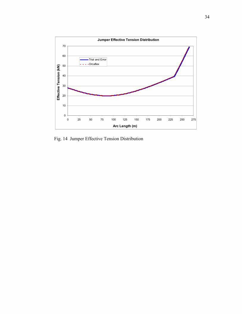
In this hypothetical case, the jumper overall length is 265 m, the horizontal span
(the horizontal distance between the jumper’s two ends) is 200 m, and vertical span (the
vertical distance between the jumper’s two ends) is 80 m. By applying the trial and error
approach, we calculated 1T =28 kN, and
1θ =45.4 o. The jumper static configuration and
effective tension distribution are as shown in Figs. 13 and 14 respectively. As a

33
validation of this approach, the results calculated by a commercial software tool
(Orcaflex) are also presented. The comparisons show good agreements on both the
jumper catenary shape and effective tension distribution. The jumper catenary shape
shows a kink at the mean surface line (vertical axis=0) because of the jumper apparent
weight discontinuity. For the same reason, the effective tension distribution also shows a
sharp turn at the mean surface line.
The static configuration was fed into the dynamic VIV simulations as the initial
boundary condition. And the jumper effective tension was applied to the modal analysis.
Jumper Static Configuration
-100
-75
-50
-25
0
25
50
0 20 40 60 80 100 120 140 160 180 200
Horizontal Axis (m)
Vertical Axis (m)
Trial and Error
Orcaflex
Fig. 13 Jumper Static Configuration
34
Jumper Effective Tension Distribution
0
10
20
30
40
50
60
70
0 25 50 75 100 125 150 175 200 225 250 275
Arc Length (m)
Effective Tension (kN)
Trial and Error
Orcaflex
Fig. 14 Jumper Effective Tension Distribution

35
VIV Response Modal Extraction
The riser modal frequencies and modal shapes can be calculated numerically.
Usually the riser (or flexible jumper) modal shapes are not orthogonal to each other
unless ii wdsdT =/ =0. This can be demonstrated as following derivation.
We start from the linearized riser dynamic motion equation, which is given by
Eq. (2). To include the catenary riser (jumper) situation, we replaced the parameter x by
the curve length parameter s. Also we are specifically concerned in cross flow direction,
and replaced y with z, as shown in Eq. (25).
zDzmfds
zdEI
ds
d
ds
dT
ds
dz
ds
zdT sz
&&& .2
2
2
2
2
2
+=+
−+ , (25)
where T is the riser effective tension, EI is the riser bending stiffness, fz is the external
force, m is the riser unit mass, and Ds is the riser structural damping. z is defined as the
cross flow direction (+z up, -z down). s is the riser (jumper) curve length measured from
the one end. Eq. (25) can be discretized using finite difference scheme:
h
zz
ds
dzn
j
n
j
2
11 −+ −= ,
2
11
2
2 2
h
zzz
ds
zdn
j
n
j
n
j −+ +−= ,
4
2112
4
4 464
h
zzzzz
ds
zdn
j
n
j
n
j
n
j
n
j −−++ +−+−= ,
2
21
2
2 2
τ
−− +−=
n
j
n
j
n
j zzz
dt
zd,
τ
1−−=
n
j
n
j zz
dt
dz,
36
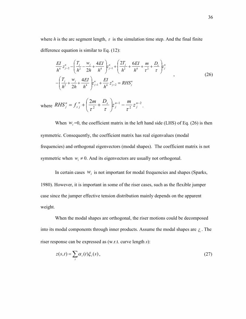
where h is the arc segment length, τ is the simulation time step. And the final finite
difference equation is similar to Eq. (12):
n
j
n
j
n
j
jj
n
jsjn
j
jjn
j
RHSzh
EIz
h
EI
h
w
h
T
zDm
h
EI
h
Tz
h
EI
h
w
h
Tz
h
EI
=+
++−
++++
+−−
++
−−
24142
24214224
4
2
624
2 ττ , (26)
where 2
2
1
2
2 −− −
++= n
j
n
j
sn
jz
n
j zm
zDm
fRHSτττ
.
When iw =0, the coefficient matrix in the left hand side (LHS) of Eq. (26) is then
symmetric. Consequently, the coefficient matrix has real eigenvalues (modal
frequencies) and orthogonal eigenvectors (modal shapes). The coefficient matrix is not
symmetric when ≠iw 0. And its eigenvectors are usually not orthogonal.
In certain cases iw is not important for modal frequencies and shapes (Sparks,
1980). However, it is important in some of the riser cases, such as the flexible jumper
case since the jumper effective tension distribution mainly depends on the apparent
weight.
When the modal shapes are orthogonal, the riser motions could be decomposed
into its modal components through inner products. Assume the modal shapes are iξ . The
riser response can be expressed as (w.r.t. curve length s):
∑=i
ii sttsz )()(),( ξα , (27)
37
where iα is the modal response amplitude, and is a real value. It can also be expressed
as complex value as Lucor et al. (2006). When iw =0, the modal shapes are orthogonal,
i.e. ji ξξ * =0 for ji ≠ , and represents the inner product of two vectors. Therefore,
( ) ( , ) /i i i it z s tα ξ ξ ξ= ∗ ∗ . When ≠iw 0, the least squares method can be used to
extract the modal response amplitudes. Let [ ]nξξξ ...21=Λ , where n is the
maximum modal shapes considered in the calculation. Λ has a dimension of N x n, and
N>n. The modal response amplitudes are then expressed as:
[ ] ( ) ),(...1
21 tszTTT
n ΛΛΛ=−
ααα . (28)
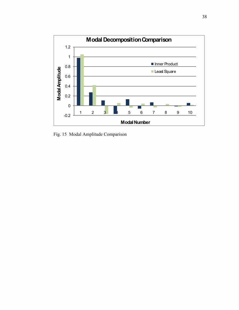
As an illustration, let )sin(),( stsz = , and Fig. 15 shows the decomposed modal
response amplitude comparisons for the 265 m jumper case. The first 10 modes were
used in the calculations. Both the inner product and the least squares methods show that
the first mode has the largest response amplitude. And the modal amplitudes decrease as
the modal number gets higher. Both methods would yield the same results if the jumper
modal shapes were orthogonal. The difference confirms that the effect of iw cannot be
neglected during jumper VIV simulation.
38
-0.2
0
0.2
0.4
0.6
0.8
1
1.2
1 2 3 4 5 6 7 8 9 10
Modal Amplitude
Modal Number
Modal Decomposition Comparison
Inner Product
Least Square
Fig. 15 Modal Amplitude Comparison

39
Jumper Transient Response
For long cylinder VIV simulation in 3D, the cylinder motion is complicated by
many factors. Transient effect is one of them. Transient effect is not only introduced by
the startup of the numerical simulation (when the cylinder is suddenly exposed to a
current), but also continuously excited through the mean position (in-line direction)
fluctuations, and kinetic energy redistribution among different modes. This section
presents an approach that could be used to estimate the jumper (or other similar catenary
risers) transient response, hence filter it from the jumper cross flow motions.
The jumper response to an impulse force is first studied. A constant load of 100
kg is applied to the 265 m jumper vertex at t=0, and then removed after t=1s, as shown
in Fig. 16. The jumper will first deform due to the impulse load, and then experience free
vibration after that. The jumper motion amplitude decays to 10% of its initial amplitude
after 70 seconds. The riser motion time histories at each node between t=30s and 60s
were used for modal extraction. And the modal response root-mean-square (rms) were
calculated and normalized by the fundamental modal response rms. Then the data were
plotted against the normalized modal frequency (fi / f1) as shown in Fig. 17. The data
distribution could be approximated by a simple exponential function:
1/1
1
ff
iiermsrms
−⋅= .
The good approximation of the exponential function provides a possible method
to eliminate the transient response from the jumper cross flow response. The procedures
are as follows:

40
1. Perform the jumper VIV simulations in time domain.
2. Extract the modal response for all modes in the study ranges through least
squares method.
3. Estimate the model response due to transient effect through exponential
function approximation.
4. Filter the transient response from the total motion. The filtered response rms
is: 22
transienttotalfiltered rmsrmsrms −= .
Note that this approach is mainly based on observations on the jumper transient
response, and its validity on other riser configurations (other than the catenary
arrangement) needs to be investigated on case-by-case basis.
F=100kg
jumper
MeanSurface Line
Fig. 16 Jumper Deformation under Impulse Load

41
0
0.2
0.4
0.6
0.8
1
1.2
0 1 2 3 4 5 6 7 8 9 10
Norm
alized Modal Response
Normalized Modal Frequency
Modal Response RMS Distribution
rms
Curve Fitting
Fig. 17 Jumper Response Distribution

42
Integration of Riser Motion Solver to Parallel Fluid Solver
The riser VIV simulations presented in this dissertation were mainly performed
using a single processor computer, i.e. all the computations by the fluid solver and riser
motion solver used only one processor. However, recently the fluid solver of the FANS
codes were expanded to parallel computation, and allowed for utilizing the multi-
processor cluster. This section is to document the details of integration of the riser
motion solver to the parallel version of the FANS codes.
In most of the practical riser VIV simulations, it is sufficient to discretize the
riser string into a total element of less than 1000. Comparing to the total element number
of the fluid domain (more than 1 million), it is negligible. And its computational effort is
also insignificant. Therefore, it is reasonable that only one processor will handle the riser
motion solver itself, i.e. all the riser motion computations will be carried out on the
master processor.
The integration of the riser motion solver to the FANS parallel version includes
the following tasks:
1. Locate the drag and lift force calculation codes in the parallel version, and
implant new codes to output the drag and lift forces along the riser. In the
force_moment module, additional codes were added to compute the forces at
each different layer, i.e. k=1..nk if k is the riser spanwise dimension, on riser
surface. The riser surface has a surface identification number of 3 or 4, i.e.
i=1..ni, and j=1. The viscous friction force and pressure induced force were
integrated on each cell, and on each processor. MPI_BARRIER subroutine

43
was called after the calculation to synchronize the computations on different
processors, and MPI_REDUCE subroutines were called to sum up the total
forces. Finally, the drag and lift coefficients were normalized from the drag
force and lift force. And this normalization was carried out by the master
processor only. The drag and lift coefficients were saved into a global array,
which could be accessed from the motion solver subroutine to solver for the
riser dynamics.
2. Locate the riser motion calculation section (2D), and replace it with 3D
motion calculation codes (direct integral motion codes). The riser motion
codes were implemented into the grid_motion module. Additional input data
for riser motion calculation was listed in data file “riser.inp”. The additional
data includes a motion solver identification number (“motion”), characteristic
length (“charl”), characteristic current velocity (“charu”), actual current
velocity, and riser sectional properties.
3. Locate the data grid movement codes, and revise the codes to move the data
grids based on riser 3D displacement. The riser motions were computed on
the master processor only. However, the motion results were broadcasted to
all processors through subroutine MPI_BCAST. The data grids then moved
based on the riser instantaneous positions on each processor. Note that the
data grid at each riser station has the same movement as the riser at that
location.
44
A test case has been selected to confirm the successful integration of the riser
motion solver to the parallel fluid solver. The selected riser configuration has following
parameters:
• Riser length 9.63 m, diameter 0.02 m, top tension 817 N, unit mass 0.7 kg/m.
• Uniform current with speed of 0.42 m/s.
• Data grid consists of : (1) body grid 182 x 35 x 50, total node number
318,500, (2) wake grid 121 x 101 x 50, total node number 611,050, (3)
background grid 121 x 91 x 50, total node number 544,500. The dimension in
riser spanwise direction is 50, or 50 stations along the riser.
• Riser is vertically positioned with pin connections at both ends.
Three cases with different processor number were considered:
1. Single processor. In this case the fluid domain of all data grids were
computed on one processor. This is equivalent to the serial code, and no
parallel computation at all.
2. Two processors. In this case, the fluid domains of the body grid and wake
grid were computed by the master processor, and the fluid domain of the
background grid was computed by a second processor. The riser motions
were solved on the master processor only.
3. Three processors. In this case, the fluid domain of the body grid was
computed by the master processor, the fluid domain of the wake grid was
computed by a second processor, and the fluid domain of the background grid

45
was computed by a third processor. The riser motions were solved on the
master processor only.
Theoretically there is no limit on the processor number used for the CFD
simulations. However, the data grids must be divided into smaller segments in order to
utilize more processors. In other words, the maximum processor number could be
utilized is the total data grid number, where each processor is assigned only one data
grid. To achieve the minimum computational time, it is recommended to distribute the
data grids to each processor with similar total nodal number. This would ensure the work
load on each processor is roughly the same, and reduce the processor idle time.
The simulation results are presented in Appendix A. It is found that the parallel
version of the FANS codes (with the riser motion solver integrated) functioned well, and
provided similar cross flow response as the serial version. The minor discrepancy is due
to the fluid solver difference: the fluid solver in the parallel version adopted an improved
velocity-pressure iteration algorithm. The results also confirmed that the computational
time could be significantly reduced by using the parallel computational techniques.

46
CHAPTER III
2D SIMULATION OF FLOW PAST A FIXED/VIBRATING RISER
Interference is an important design consideration for deepwater applications. In
many design practices no collisions are allowed between objects such as risers,
flowlines, umbilicals, tendons/mooring lines, and hull structures. Among them
interference between top tensioned risers is of particular interest. The reason is that top
tensioned riser array has strict limitations on surface wellheads layout and subsea
wellhead layout. When water depth reaches 10,000ft, the riser string experiences much
larger lateral displacement due to current force. To avoid riser clashing, a very large
subsea wellhead pattern might be required. This would impose challenges to riser system
design, especially when large quantity of top tensioned risers is planned (Huang and
Chen, 2006).
In conventional design approach (API RP 2RD, 1998), riser interference analysis
is usually carried out quasi-statically. The wake field behind the upstream riser is
calculated by using Huse’s formula (Huse 1993, 1996). The VIV induced drag
coefficient amplification of upstream riser is approximated by multiplying the base drag
coefficient by an amplification factor. And an effective drag diameter is used to calculate
the wake field behind the upstream riser undergoing VIV. This approach is simple and
straightforward. However, it might also introduce conservatism and uncertainty into the
design. Consequently, it is desirable to evaluate the VIV effect on upstream riser
effective drag coefficient and wake field.
47
Therefore, the analysis results presented in this section is served as following
purposes:
1. Compare the wake flow field to the experimental data (Huse’s formula) and
validate the data grids and CFD approach.
2. Discover localized features of the flow fields that are not included in the
Huse’ formula.
3. Provide a riser interference example case and illustrate the significance of the
findings.
In this simulation the effective drag coefficients and wake fields are obtained for
both fixed riser and vibrating riser. The Reynolds number was chosen as 3x10⁵. A study
case is selected with typical Gulf of Mexico 10-year loop current and a typical single
casing production riser. The riser system data, including air weight, submerged weight,
and top tensions, are then developed. In the example case, the riser interference analysis
is performed based on the obtained effective drag coefficients, and the results are
compared to those obtained by Huse’s formula.
Data Grid
Overset grid (Chimera) technique provides an effective way to handle riser
movement. Figs. 18 and 19 show the data grids used in this study. The body grid has a
dimension of 182x41x12, while the background grid has a dimension of 201x101x12.
The data grids have been delicately generated with very fine grid sizes at the riser
boundary layer and vortex shedding zones. The body grid and background grid are
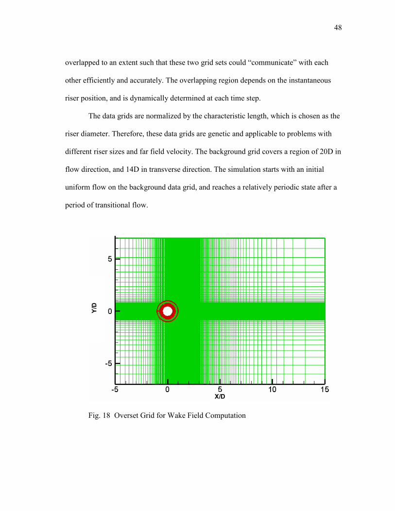
48
overlapped to an extent such that these two grid sets could “communicate” with each
other efficiently and accurately. The overlapping region depends on the instantaneous
riser position, and is dynamically determined at each time step.
The data grids are normalized by the characteristic length, which is chosen as the
riser diameter. Therefore, these data grids are genetic and applicable to problems with
different riser sizes and far field velocity. The background grid covers a region of 20D in
flow direction, and 14D in transverse direction. The simulation starts with an initial
uniform flow on the background data grid, and reaches a relatively periodic state after a
period of transitional flow.
X/D
Y/D
Fig. 18 Overset Grid for Wake Field Computation

49
Riser
Grid attached to Riser
Background Fixed Grid
Fig. 19 Overset Grid for Wake Field Computation – Riser Surface Vicinity
Riser Interference Analysis Procedures
The riser interference is checked by using a quasi-static approach under typical
10-year loop current profile in Gulf of Mexico. The effective drag coefficients of the
downstream risers are calculated based on obtained wake field. The analysis procedures
are as shown in Fig. 20. Since at the beginning both of the downstream riser deflection
and effective drag coefficients are unknown, initial assumptions are needed to start the
iterations. The riser string is divided into small segments. Each segment has its own
effective drag coefficient, which is calculated based on Huse’s formula or CFD
approach. Both of them are used in this section, and the results are compared as well. In
the CFD approach, a more accurate way is to position two risers in the same

50
computational domain, and compute the effective drag coefficients on both risers
directly. However, this would require a CFD simulation on each different riser position
pairs, and introduce tremendous computational effort, hence it is not adopted here.
Upstream Riser VIV
A/D and mode
Wake Field behind
Upstream Riser
Upstream Riser
Dynamic Simulation
Upstream Riser
Effective Cd
Downstream Riser
Effective Cd
Upstream Riser
Lateral Deflection
Downstream Riser
Lateral Deflection
Clearance Check
Converged?
Y
N
Fig. 20 Riser Interference Analysis Flow Chart
Simulation Results
A typical 10 ¾” single casing production riser has been sized for 10,000ft water
depth as shown in Table 2. Conventional hydro-pneumatic tensioners are assumed, and
pipe properties were obtained from API 5L (2000) and API 5C3 (1994).
Table 2 10 ¾” Riser Top Tensions
Nominal To
Wet Wt Riser Type Riser Mode
(kips) (kips)
TF
Normal Operating 1026 769 1.34 10 3/4" Single Casing Riser
Well Killed 1350 1036 1.31
51
The riser clearance is checked in 10-yr loop current condition in Gulf of Mexico.
The current profile has a maximum speed of about 3 knots at 1,500 ft below the mean
sea surface. In this section the upstream riser VIV a/D and frequency are calculated by
using a separate VIV analysis tool as:
• Single mode excited: 86th,
• a/D=0.28,
• Frequency = 1.6Hz.
The upstream riser is assumed to be in heavy mode (well killed) and with VIV.
The downstream riser is assumed in normal operating condition and without VIV.
Typical riser spacing at the topsides wellbay is used. The riser spacing on the sea floor is
usually a design parameter. Here we chose this parameter based on previous TLP project
experience with water depth extrapolation.
Simulations have shown a rapidly varying effective drag coefficient within each
vortex shedding and riser vibrating cycle. Considering the varying frequency is high, the
riser vibrating amplitudes in the current plane (in-line vibration) is expected to be small.
Therefore, time averaged mean drag coefficients are used to calculate the riser
deflections. This quasi-static approach is valid if the clearance satisfies certain minimum
value.
Fig. 21 shows the flow field vorticity contours for fixed riser. Figs. 22 and 23
show the comparisons of the wake field velocity distributions by using Huse’s formula
and CFD approach. The comparisons show very good agreement. It also confirms the

52
validity of the CFD approach. Fig. 24 provides the time history of the effective drag
coefficient. It has a mean value of 1.0, which is consistent with published Cd vs Re
curve and design codes such as API RP 2RD.
Fixed Riser Vorticity Contour, t=20.0s Fixed Riser Vorticity Contour, t=20.4s
Fixed Riser Vorticity Contour, t=20.8s Fixed Riser Vorticity Contour, t=21.2s
Fixed Riser Vorticity Contour, t=21.6s Fixed Riser Vorticity Contour, t=22.0s
Fig. 21 Vorticity Contours for Fixed Riser

53
Fig. 22 Wake Field 3D View – Top:Huse’s Formula, Bottom:CFD
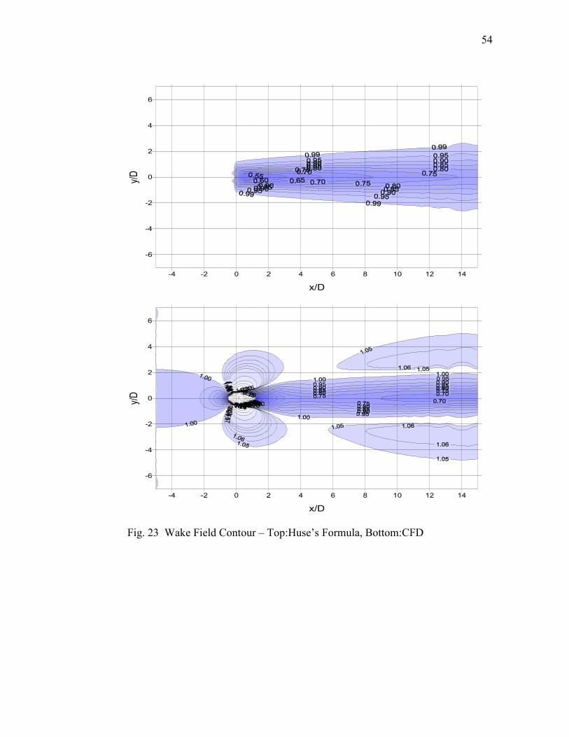
54
-4 -2 0 2 4 6 8 10 12 14
x/D
-6
-4
-2
0
2
4
6
y/D
-4 -2 0 2 4 6 8 10 12 14
x/D
-6
-4
-2
0
2
4
6
y/D
Fig. 23 Wake Field Contour – Top:Huse’s Formula, Bottom:CFD
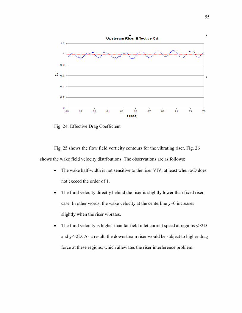
55
Fig. 24 Effective Drag Coefficient
Fig. 25 shows the flow field vorticity contours for the vibrating riser. Fig. 26
shows the wake field velocity distributions. The observations are as follows:
• The wake half-width is not sensitive to the riser VIV, at least when a/D does
not exceed the order of 1.
• The fluid velocity directly behind the riser is slightly lower than fixed riser
case. In other words, the wake velocity at the centerline y=0 increases
slightly when the riser vibrates.
• The fluid velocity is higher than far field inlet current speed at regions y>2D
and y<-2D. As a result, the downstream riser would be subject to higher drag
force at these regions, which alleviates the riser interference problem.

56
Fig. 27 presents the effective drag coefficient time history. It varies in riser
vibrating frequency, with values ranging from 0.5 to 2.8. The drag force variation is
mainly due to the pressure zone shifting on the riser surface. The averaged mean value
of 1.37 is then used for the upstream riser with VIV.
Vibrating Riser, t=22.5s Vibrating Riser, t=23.0s
Vibrating Riser, t=23.5s Vibrating Riser, t=24.0s
Vibrating Riser, t=24.5s Vibrating Riser, t=25.0s
Fig. 25 Vorticity Contours for Vibrating Riser

57
-4 -2 0 2 4 6 8 10 12 14
x/D
-6
-4
-2
0
2
4
6
y/D
Fig. 26 Wake Field behind a Vibrating Riser
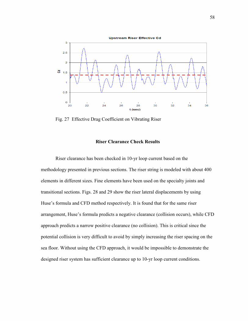
58
Fig. 27 Effective Drag Coefficient on Vibrating Riser
Riser Clearance Check Results
Riser clearance has been checked in 10-yr loop current based on the
methodology presented in previous sections. The riser string is modeled with about 400
elements in different sizes. Fine elements have been used on the specialty joints and
transitional sections. Figs. 28 and 29 show the riser lateral displacements by using
Huse’s formula and CFD method respectively. It is found that for the same riser
arrangement, Huse’s formula predicts a negative clearance (collision occurs), while CFD
approach predicts a narrow positive clearance (no collision). This is critical since the
potential collision is very difficult to avoid by simply increasing the riser spacing on the
sea floor. Without using the CFD approach, it would be impossible to demonstrate the
designed riser system has sufficient clearance up to 10-yr loop current conditions.

59
TTR Lateral Displacements
0
5
10
15
20
25
30
35
40
45
50
0 1,000 2,000 3,000 4,000 5,000 6,000 7,000 8,000 9,000 10,000
Elevation from Mudline (ft)
Lateral Displacement (ft)
10.75" OD Production Riser - well killed
10.75" OD Production Riser - normal operating
Fig. 28 Riser Displacement along Riser – Huse’s Formula
TTR Lateral Displacements
0
5
10
15
20
25
30
35
40
45
50
0 1,000 2,000 3,000 4,000 5,000 6,000 7,000 8,000 9,000 10,000
Elevation from Mudline (ft)
Lateral Displacement (ft)
10.75" OD Production Riser - well killed
10.75" OD Production Riser - normal operating
Fig. 29 Riser Displacement along Riser – FANS

60
Discussions
This section preliminarily studied the ultra deepwater riser interference by using
an unsteady, overset-grid (Chimera), incompressible Navier-Stokes (RANS) method. It
is found that risers could have very large lateral deflections in strong and deep currents,
and riser interference could impose serious challenges to riser system design. Under
certain design conditions, such as 10-yr loop current eddy as studied in this section, the
riser interference results are sensitive to drag coefficients. Therefore, accurate
assessment of the effective drag coefficients on both the upstream and downstream riser
becomes critical. The CFD time domain simulation approach has predicted a narrow
wake field and a high-speed zone outside the wake field. Both of them positively
affected the interference results. It is also indicated that the “no collision” design criteria
could be hold up to 10-yr extreme current events in ultra deep water riser systems
(Huang and Chen, 2006).

61
CHAPTER IV
3D SIMULATION OF FLOW PAST A VERTICAL RISER
IN UNIFORM CURRENT
During the last several years many VIV experiments have been carried out on
deepwater risers with large L/D. With the some of the newly released experimental data,
it becomes possible now to extend the comparisons between CFD results and
experimental data to greater detail, such as modal response amplitudes and phase angles,
response power spectral densities (PSD), and motion trajectories, etc. In this chapter,
two uniform current profiles were chosen form the experimental database
(oe.mit.edu/VIV/) with constant speed of 0.42 m/s (test case 1105) and 0.84 m/s (test
case 1108) respectively. During the experiment, the riser was vertically positioned
under the water. Both ends were fixed to the test rig, which rotates at a constant speed.
This would simulate a uniform current condition. Note that after the rig completes one
cycle, the riser moves into its own wake field. This fluid disturbance is expected to be
negligible and not considered in the present numerical simulations (Huang et al., 2009a,
2009b).
In the present simulations, 1.5 million elements for this 10 m long top-tensioned
riser (L/D=482) were used. The riser lateral motion is solved in the time domain using
the direct integration solver. Both in-line and cross flow riser responses are computed
and compared with the published experimental data.
62
Data Grid
The simulation data grid consists of three sets of data grids and has a total of 1.5
million grid points. The three sets of data grids are: (1) body grid – the data grid adjacent
to the riser surface that provides fine resolution to calculate the fluid-riser surface
interaction and vortex generation, it has dimensions of 50 x 182 x 35, (2) wake grid – it
interfaces with body grid and background grid and provides good resolution for vortex
propagation, it has dimensions of 50 x 121 x 101, (3) background grid – as the name
suggests, it defines the outer boundary of the computational fluid domain, provides the
far field fluid boundary conditions, interfaces with and provides a physical extension to
the wake grid using relatively coarse mesh. It has dimensions of 50 x 121 x 91. Figs. 30
and 31 show the fine meshes near the riser surface, and the overlapping region between
the body grid and wake grid. Fig. 32 shows the data grids with riser deflection (only
three layers are shown for clarity). When the riser vibrates, the data grids also move with
the riser so there is no gap between the riser and the grids at any time.
It was modeled as a beam with top tension of 817 N, and discretized using 250
segments – a typical number for riser global dynamic analysis. Its two ends are pinned to
the ground with zero rotational stiffness. Its unit mass is 0.7 kg/m, and bending stiffness
is 135 N-m. No damping has been included. It is estimated that the dominant mode
should be less than the sixth mode. The Reynolds numbers are 7.5x10³ for U=0.42 m/s
and 1.5x10⁴ for U=0.84 m/s respectively.

63
Fig. 30 Data Grids at x/L=Constant
Fig. 31 Grid Details on Riser Surface and Overlapping Region

64
Fig. 32 Data Grids with Riser Deflection

65
Simulation Results
The riser VIV responses in two uniform current profiles are analyzed. The
current speeds are U=0.42 m/s and 0.84 m/s. The corresponding experimental load case
numbers are 1105 and 1108 respectively. These two current profiles were chosen to
cover the typical current speed range that could occur in offshore fields. The cross flow
VIV is generally more important than the in-line VIV, hence it was the primary focus of
this study.
First we performed the modal analysis of the vertical riser. Table 3 shows the
natural frequencies of the riser under three conditions: (1) the riser is horizontally
positioned in the air with constant tension 817 N. Its fundamental frequency is 1.78 Hz;
(2) the riser is vertically positioned in the water, with constant added mass coefficient
Ca=1.0. Its fundamental frequency is reduced to 1.44 Hz based on averaged tension 797
N; (3) discretize the riser into segments and calculate the eigenvalues and eigenvectors,
with constant added mass coefficient Ca=1.0, and distributed tension (top 817 N, bottom
777 N). Its fundamental frequency is calculated as 1.38 Hz, which is slightly different
(5%) from condition (2). We also calculated the modal shapes. They are similar to the
sinusoidal shapes, but not exactly the same. The riser effective tension varies along the
pipe and causes the modal shapes to deviate from simple sinusoidal function, especially
for deepwater risers. The modal analysis is important because we need the modal
frequencies to assess the dominant modes, and we also need the modal shapes for almost
all the post-processing work, including modal component extraction, modal response
PSD, modal added mass, etc. In our present method the modal shapes are not involved in

66
the numerical simulations because we are using the direct integration riser solver. The
FANS codes also include a riser modal motion solver, which calculate the riser segment
instantaneous positions based on modal superposition.
Table 3 Riser Modal Frequency Summary
ϖϖϖϖ f ϖϖϖϖ f ϖϖϖϖ f
(rad/s) (Hz) (rad/s) (Hz) (rad/s) (Hz)
1 11.2 1.78 9.1 1.44 8.6 1.38
2 22.3 3.55 18.1 2.88 17.3 2.75
3 33.5 5.33 27.2 4.33 26.0 4.13
4 44.6 7.10 36.3 5.77 34.6 5.51
5 55.8 8.88 45.3 7.21 43.3 6.89
6 66.9 10.65 54.4 8.65 52.0 8.28
7 78.1 12.43 63.4 10.10 60.7 9.67
8 89.2 14.20 72.5 11.54 69.5 11.06
Mode No
In Air, 817N In Water, 817N/777N FEA Calculated
The simulations start with an initially straight riser. The riser begins to deflect
after it is exposed to a uniform current, and it deflects increasingly until its internal
restoring force is sufficiently large to overcome the drag forces. The time domain
simulations are carried out to a total of 20,000 time steps, or the fluid travels a total
distance of 200 OD (4m) for both cases. Fig. 33 shows the evolution of the riser VIV and
vortex shedding under different current profiles. The left hand side riser is undergoing
VIV in uniform current 0.42 m/s, while the right hand side riser is undergoing VIV in
uniform current 0.84 m/s. Both risers start with straight configuration. After a period
(approximately 2 seconds) of transient response, both risers reach nearly equilibrium

67
positions. The maximum riser deflection occurs at the middle section for risers in
uniform currents. The maximum riser deflection amplitude for the U=0.84 m/s case is
approximately four times of that for the U=0.42 m/s case. This is reasonable since the
drag force is proportional to the square of the current speed. The majority of the vortex
shedding shows a clear 2S pattern (Williamson and Roshko, 1988). The cross flow VIV
amplitudes are in the order of 1D. No obvious 2T patterns (Williamson and Jauvtis,
2004) have been observed in these two simulations.
Fig. 34 shows two snap shots of the vorticity contours for U=0.42 m/s and
U=0.84 m/s respectively. The riser maximum lateral deflection for U=0.84 m/s case is
approximately 20D (riser diameter), and it reduces to 5D for the U=0.42 m/s case.
Fig. 35 shows the riser deflection time history. The riser achieves its balanced
position through two steps: (1) riser deflects toward current downstream with no or
negligible cross flow VIV. In this case the drag coefficient on the riser is approximately
1.1 along the riser (time averaged); (2) the riser starts cross flow VIV. The drag
coefficient on the riser is suddenly increased due to cross flow VIV. The VIV-enhanced
drag coefficients are much higher than the initial value (or 1.1), and the exact values are
expected to be related to many parameters such as fluid conditions, x/L, etc. As a result
of the cross flow VIV, the riser deflects further downstream until a new balanced
position is reached.

68
Figs. 36 and 37 compare the riser cross flow VIV responses to the experimental
results for U=0.42 m/s and U=0.84 m/s, respectively. The comparisons show general
agreement. The CFD simulations slightly overshoot the cross flow VIV amplitudes
during the ramp-up time. A possible reason is that the riser is suddenly exposed to the
uniform current while in the experiments the test rig rotating speed is gradually
increased to the desired values. The riser motions at x/L=0.44 are compared because (1)
the experimental data were provided at this location, (2) it is near the center of the riser
and has large deflection, which is expected to be a good location for cross flow motion
comparisons. While more comparisons can be carried out at different riser locations, it is
generally more desirable to compare the rms a/D along the riser length, as discussed in
the next section.
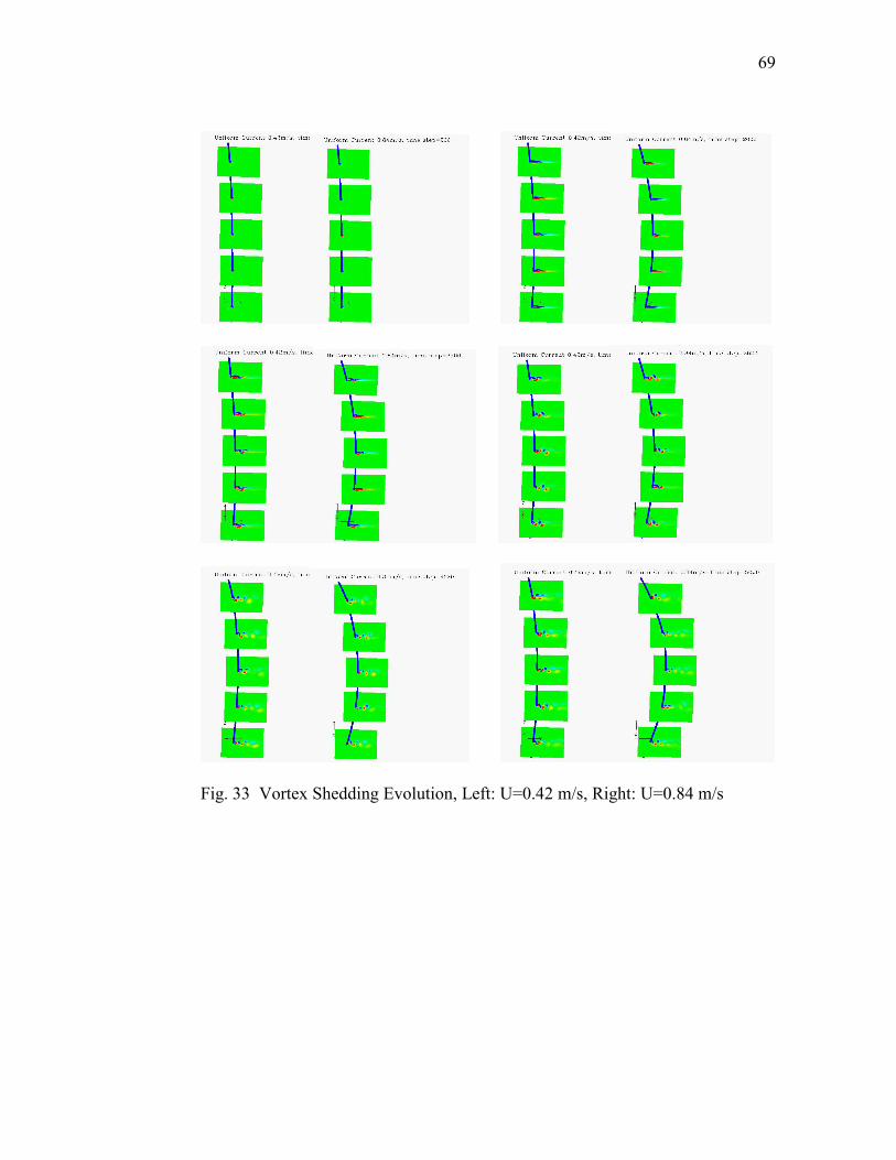
69
Fig. 33 Vortex Shedding Evolution, Left: U=0.42 m/s, Right: U=0.84 m/s
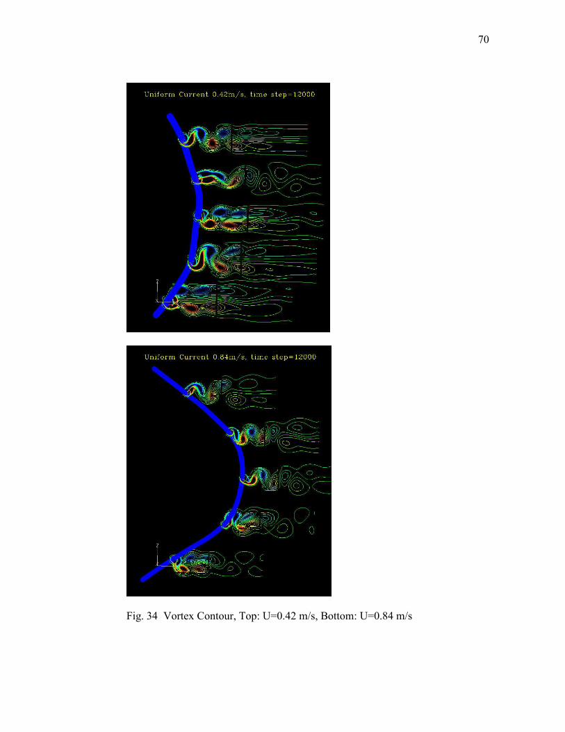
70
Fig. 34 Vortex Contour, Top: U=0.42 m/s, Bottom: U=0.84 m/s

71
Riser Deflection @ x/L=0.5
0
5
10
15
20
25
0 0.5 1 1.5 2 2.5 3 3.5 4
t (sec)
y/D U=0.84m/s
U=0.42m/s
Fig. 35 Riser Deflection Time History, x/L=0.5
Riser CF Response @ x/L=0.44
-1
-0.8
-0.6
-0.4
-0.2
0
0.2
0.4
0.6
0.8
1
0 1 2 3 4 5 6 7 8
t (sec)
z/D
FANS (U=0.42m/s)
Experiment (U=0.42m/s)
Fig. 36 Riser CF Response (U=0.42 m/s)
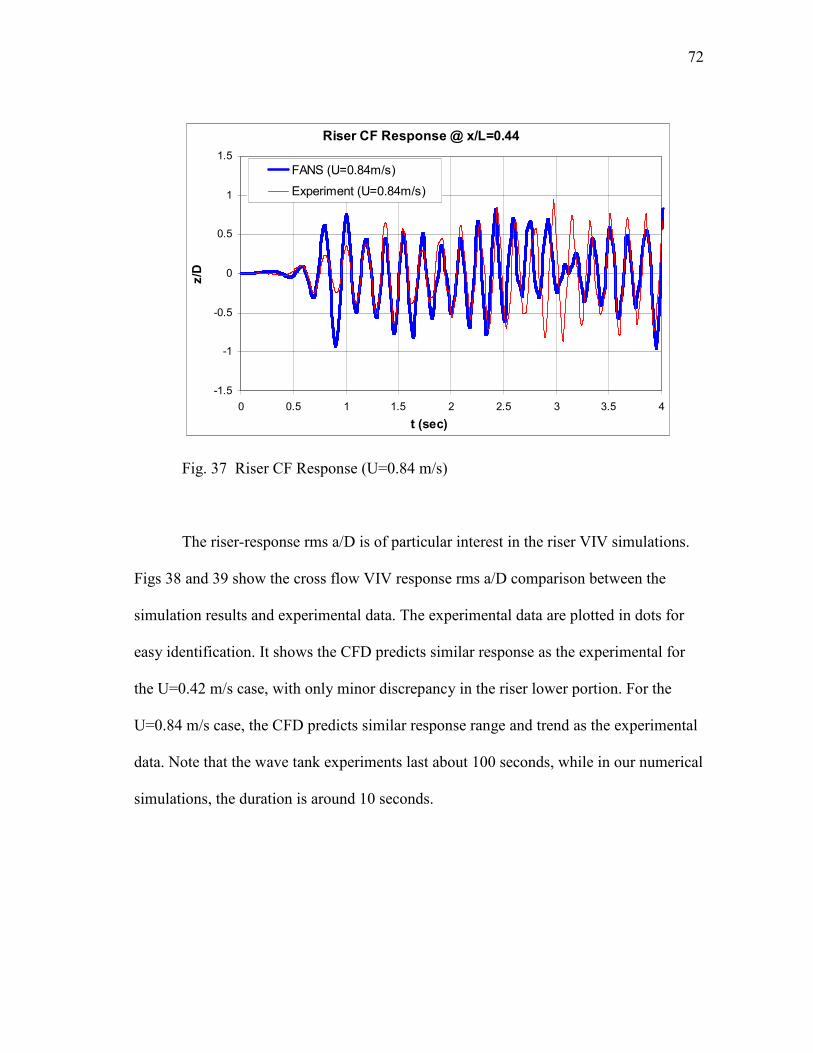
72
Riser CF Response @ x/L=0.44
-1.5
-1
-0.5
0
0.5
1
1.5
0 0.5 1 1.5 2 2.5 3 3.5 4
t (sec)
z/D
FANS (U=0.84m/s)
Experiment (U=0.84m/s)
Fig. 37 Riser CF Response (U=0.84 m/s)
The riser-response rms a/D is of particular interest in the riser VIV simulations.
Figs 38 and 39 show the cross flow VIV response rms a/D comparison between the
simulation results and experimental data. The experimental data are plotted in dots for
easy identification. It shows the CFD predicts similar response as the experimental for
the U=0.42 m/s case, with only minor discrepancy in the riser lower portion. For the
U=0.84 m/s case, the CFD predicts similar response range and trend as the experimental
data. Note that the wave tank experiments last about 100 seconds, while in our numerical
simulations, the duration is around 10 seconds.

73
CF Motion rms a/D (U=0.42m/s)
0.0
0.1
0.2
0.3
0.4
0.5
0.6
0.7
0.8
0.9
0 0.2 0.4 0.6 0.8 1x/L
rms a/D
Test 1105
CFD (FANS)
Fig. 38 Cross Flow VIV RMS a/D, U=0.42 m/s
CF Motion rms a/D (U=0.84m/s)
0.0
0.1
0.2
0.3
0.4
0.5
0.6
0 0.2 0.4 0.6 0.8 1x/L
rms a/D
Test 1108
CFD (FANS)
Fig. 39 Cross Flow VIV RMS a/D, U=0.84 m/s

74
For illustration, the riser movement trajectories for uniform current U=0.42m/s
are shown in Figs. 40 and 41. We compared the riser motions at x/L=0.44, which is in
the middle section of the riser. In 3D simulations, the riser usually has large deflection in
flow direction due to mean drag force. And fluctuations of Cd impact the maximal
displacements in z direction as well as y direction. Therefore, the riser motion
trajectories show more complexity or randomness than 2D simulations. In our
comparisons both the CFD and experiment show similar motion trajectory – deformed
figure “8”.
Riser Motion Trajectory @ x/L=0.44
-0.5
-0.4
-0.3
-0.2
-0.1
0
0.1
0.2
0.3
0.4
0.5
-0.25 -0.2 -0.15 -0.1 -0.05 0 0.05 0.1 0.15
(y-ymean)/D
z/D
FANS (U=0.42m/s)
Fig. 40 Riser Motion Trajectory Comparison (CFD)

75
Riser Motion Trajectory @ x/L=0.44
-0.8
-0.6
-0.4
-0.2
0
0.2
0.4
0.6
0.8
-0.3 -0.2 -0.1 0 0.1 0.2 0.3
(y-ymean)/D
z/D
Experiment (U=0.42m/s)
Fig. 41 Riser Motion Trajectory Comparison (Experimental Data)
Higher harmonics refer to the VIV high frequency components having integer
multiple numbers of the cross flow or the in-line VIV frequency. It has been observed
and measured during actual drilling operations (Tognarelli et al., 2008). Our numerical
simulations provide a good tool to investigate this higher harmonics. We plotted the lift
coefficient time histories for U=0.42 m/s and U=0.84 m/s, as shown in Figs. 42 to 45 .
The lift coefficients are plotted in two locations on riser: x/L=0.3 and x/L=0.5. In those
figures we noticed the lift coefficient time histories show the third high frequency
component (3x). This indicates that the 3x harmonics could be related to the vortex
shedding patterns and lift force. Fig. 46 shows the cross flow VIV PSD of the
experimental data 1105. There are three peaks on the PSD graph: the cross flow
dominant mode (first peak), in-line VIV (second peak), and the higher harmonics (third

76
peak). Fig. 47 is the plot of the cross flow VIV PSD of the CFD simulation U=0.42 m/s.
It shows the same peaks, with the same frequencies as the experiments. The PSD from
the CFD simulation appears to have much larger band width than the experimental data.
This is due to the different time history durations for FFT analysis. The experimental
data covers a fairly long duration (~100seconds) while the CFD simulations are
relatively short (<10seconds). Therefore, the frequency resolution (dω) for the CFD
simulation PSDs are 10 times coarser than that of the experimental data. This explains
that the PSDs of the CFD simulations are wider and shorter than that of the experiments
while the total energies are about the same. Theoretically the steady VIV response PSDs
consist of a series of Dirac delta functions centered at each modal frequencies. In other
words, only the response energies and frequencies are important. The band width of the
PSDs is meaningless and does not impact the major conclusions. Figs. 48 and 49 repeat
the same information for the U=0.84 m/s case. It confirms (1) the existence of the higher
harmonics, and (2) the validity of using CFD time-domain simulation for further study.
It is interesting to see that, based on the observation from these figures, the lift
coefficients show fairly strong response at higher frequency harmonics, such as 3x.
However, the motions do not show same level of the response. One possible reason is
that the lift forces are acting on the riser segments locally, while the riser cross flow VIV
response depends on the integrated effect of all the segments. Therefore, if the high
frequency lift forces are out-of-phase with each other, then they would cancel each other
and the higher harmonics would be weak. If the lift forces were synchronized along the
riser, then we would expect very strong higher harmonics. Further investigation is
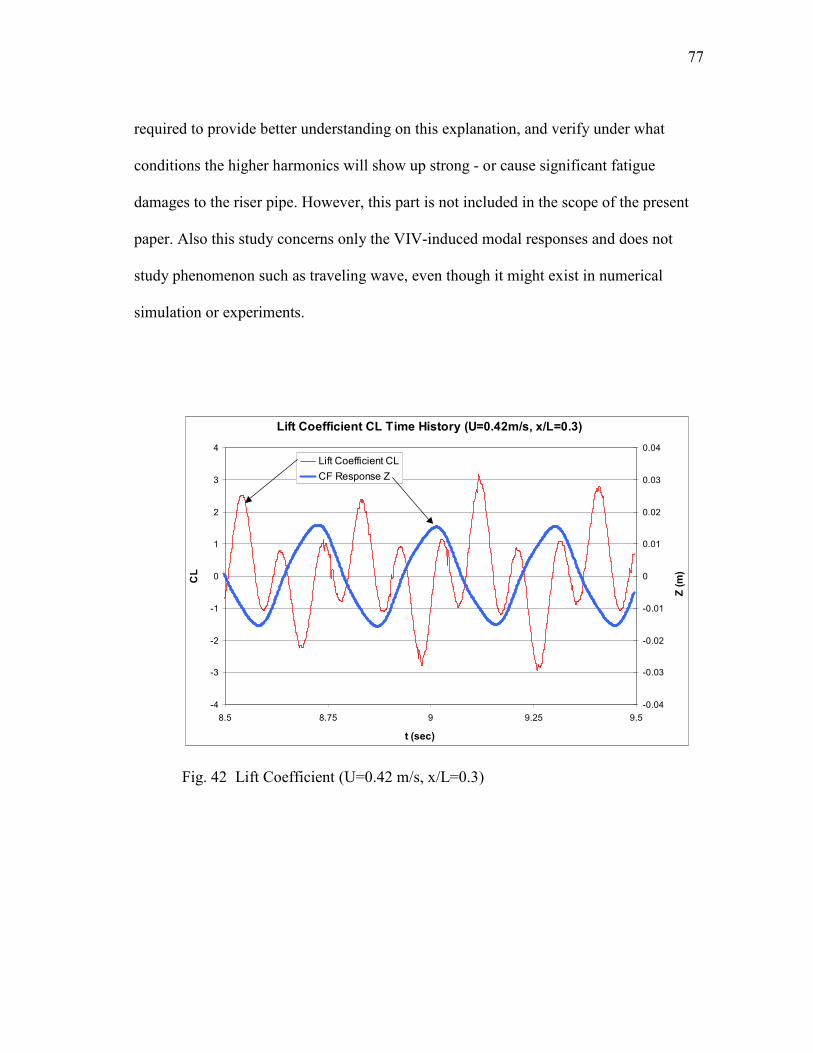
77
required to provide better understanding on this explanation, and verify under what
conditions the higher harmonics will show up strong - or cause significant fatigue
damages to the riser pipe. However, this part is not included in the scope of the present
paper. Also this study concerns only the VIV-induced modal responses and does not
study phenomenon such as traveling wave, even though it might exist in numerical
simulation or experiments.
Lift Coefficient CL Time History (U=0.42m/s, x/L=0.3)
-4
-3
-2
-1
0
1
2
3
4
8.5 8.75 9 9.25 9.5
t (sec)
CL
-0.04
-0.03
-0.02
-0.01
0
0.01
0.02
0.03
0.04
Z (m)
Lift Coefficient CL
CF Response Z
Fig. 42 Lift Coefficient (U=0.42 m/s, x/L=0.3)

78
Lift Coefficient CL Time History (U=0.42m/s, x/L=0.5)
-4
-3
-2
-1
0
1
2
3
4
8.5 8.75 9 9.25 9.5
t (sec)
CL
-0.04
-0.03
-0.02
-0.01
0
0.01
0.02
0.03
0.04
Z (m)
Lift Coefficient CL
CF Response Z
Fig. 43 Lift Coefficient (U=0.42 m/s, x/L=0.5)
Lift Coefficient CL Time History (U=0.84m/s, x/L=0.3)
-4
-3
-2
-1
0
1
2
3
4
3.5 3.75 4 4.25 4.5
t (sec)
CL
-0.04
-0.03
-0.02
-0.01
0
0.01
0.02
0.03
0.04
Z (m)
Lift Coefficient CL
CF Response Z
Fig. 44 Lift Coefficient (U=0.84 m/s, x/L=0.3)

79
Lift Coefficient CL Time History (U=0.84m/s, x/L=0.5)
-4
-3
-2
-1
0
1
2
3
4
3.5 3.75 4 4.25 4.5
t (sec)
CL
-0.04
-0.03
-0.02
-0.01
0
0.01
0.02
0.03
0.04
Z (m)
Lift Coefficient CL
CF Response Z
Fig. 45 Lift Coefficient (U=0.84 m/s, x/L=0.5)
CF Motion PSD (Test 1105, U=0.42m/s)
0.0E+00
5.0E-03
1.0E-02
1.5E-02
2.0E-02
2.5E-02
0 10 20 30 40 50 60
w (rad/s)
CF Response PSD (m^2-s/rad)
2nd
1st
3rd
Fig. 46 CF Motion PSD (Experiment 1105)
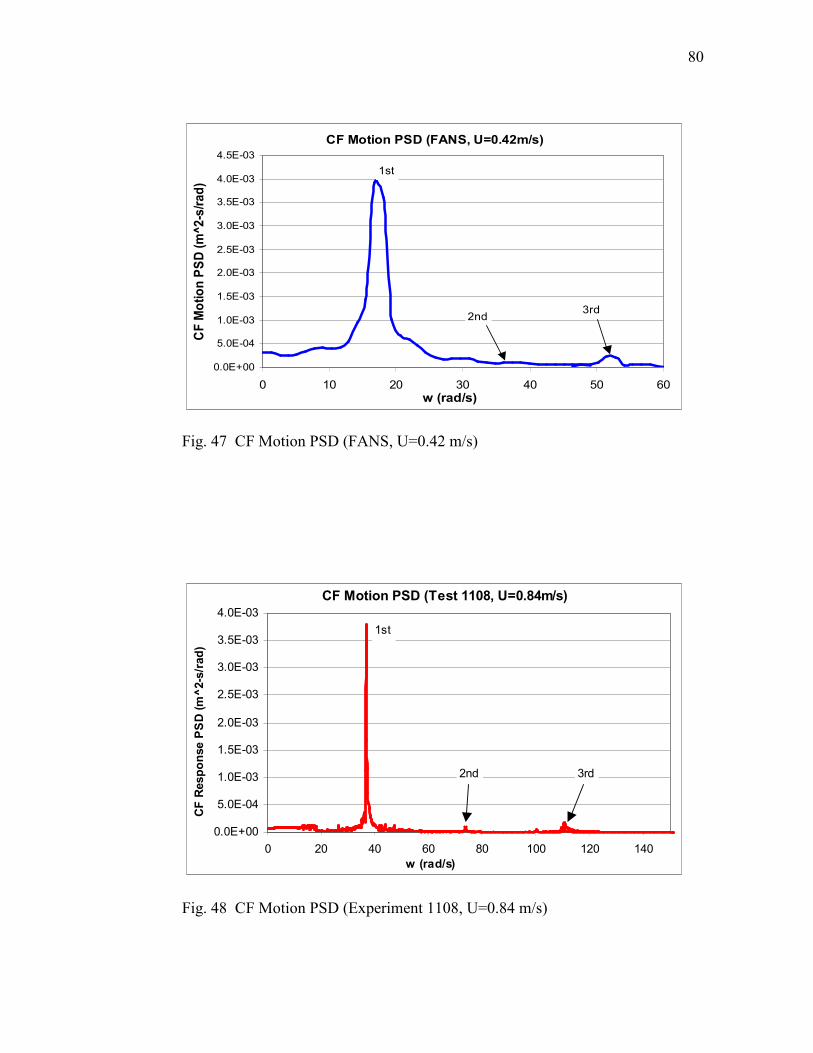
80
CF Motion PSD (FANS, U=0.42m/s)
0.0E+00
5.0E-04
1.0E-03
1.5E-03
2.0E-03
2.5E-03
3.0E-03
3.5E-03
4.0E-03
4.5E-03
0 10 20 30 40 50 60w (rad/s)
CF Motion PSD (m^2-s/rad)
1st
3rd2nd
Fig. 47 CF Motion PSD (FANS, U=0.42 m/s)
CF Motion PSD (Test 1108, U=0.84m/s)
0.0E+00
5.0E-04
1.0E-03
1.5E-03
2.0E-03
2.5E-03
3.0E-03
3.5E-03
4.0E-03
0 20 40 60 80 100 120 140
w (rad/s)
CF Response PSD (m^2-s/rad)
2nd
1st
3rd
Fig. 48 CF Motion PSD (Experiment 1108, U=0.84 m/s)
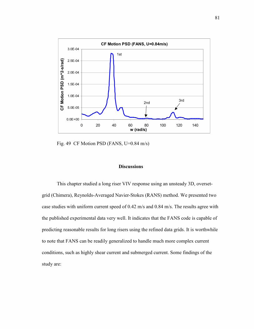
81
CF Motion PSD (FANS, U=0.84m/s)
0.0E+00
5.0E-05
1.0E-04
1.5E-04
2.0E-04
2.5E-04
3.0E-04
0 20 40 60 80 100 120 140w (rad/s)
CF Motion PSD (m^2-s/rad)
1st
3rd2nd
Fig. 49 CF Motion PSD (FANS, U=0.84 m/s)
Discussions
This chapter studied a long riser VIV response using an unsteady 3D, overset-
grid (Chimera), Reynolds-Averaged Navier-Stokes (RANS) method. We presented two
case studies with uniform current speed of 0.42 m/s and 0.84 m/s. The results agree with
the published experimental data very well. It indicates that the FANS code is capable of
predicting reasonable results for long risers using the refined data grids. It is worthwhile
to note that FANS can be readily generalized to handle much more complex current
conditions, such as highly shear current and submerged current. Some findings of the
study are:

82
1. The vortex shedding pattern in the uniform current is mainly within the “2S”
category, while its appearance varies significantly at different elevations
along the riser.
2. Mode lock-in occurs in both uniform current cases. The cross flow VIV
dominant frequency is similar to the riser in-water natural frequency. In other
words, the modal added mass coefficients of the dominant modes are around
1.0. However, the modal added mass coefficients for non-dominant modes
could vary. It is also an area deserves further study.
3. Higher harmonics have been observed in both the experimental data and the
CFD numerical simulations. It is likely the 3x higher harmonics is due to the
lift force high frequency components, hence the vortex shedding pattern.
Further investigation is required to disclose more details on this relationship,
and evaluate the impact on riser fatigue and associated mitigation options.
In conclusion, we used a CFD approach to simulate a large L/D riser VIV
response in uniform current. The simulation details are presented, analyzed, and
validated against the experimental data. Furthermore, it is also an effective tool for
disclosing insightful data and pictures that could lead to problem identification and
solutions in the riser-fluid interaction area (Huang et al. 2007a, 2007b, 2007c, 2007d).
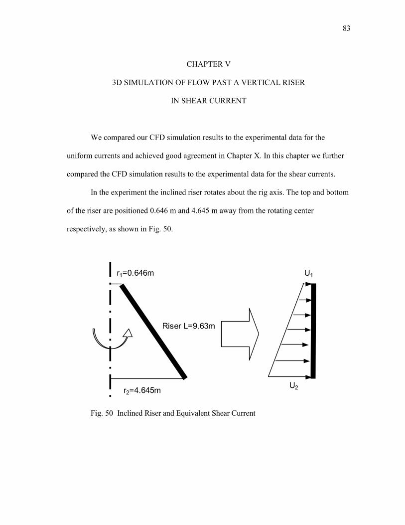
83
CHAPTER V
3D SIMULATION OF FLOW PAST A VERTICAL RISER
IN SHEAR CURRENT
We compared our CFD simulation results to the experimental data for the
uniform currents and achieved good agreement in Chapter X. In this chapter we further
compared the CFD simulation results to the experimental data for the shear currents.
In the experiment the inclined riser rotates about the rig axis. The top and bottom
of the riser are positioned 0.646 m and 4.645 m away from the rotating center
respectively, as shown in Fig. 50.
Riser L=9.63m
r1=0.646m
r2=4.645m
U1
U2
Fig. 50 Inclined Riser and Equivalent Shear Current
84
The shear current speed has a linear profile with U1 at top and U2 at bottom,
where U1/U2=0.14. The two cases we selected for comparison are U2=0.42m/s (test case
#1205) and U2=0.84m/s (test case #1210). During the experiment, the riser was
positioned under the water. Both ends were pinned to the test rig, which rotates at a
constant angular velocity. This would simulate a linearly shear current condition. Note
that after the rig completes one cycle, the riser moves into its own wake field. This fluid
disturbance is expected to be negligible and not considered in our numerical simulations.
Simulation Results
The vortex shedding and riser motions are visualized for all the simulations. Fig.
51 shows some of the video frames illustrating the riser deflections and axial vorticity
contours. Nearly all of the vortices follow “2S” pattern. The vortices develop at the riser
bottom first because it is subject to the highest current speed. The risers have in-plane
deflection due to the current induced drag force. The largest deflection is less than 10D,
which is relatively small comparing to the L/D (=482) and validates the tensioned beam
equation for riser motion calculation. For the case U2=0.42 m/s, the 2nd mode dominates
the cross flow VIV. While for the case U2=0.84 m/s, the 4th mode is dominant. The riser
has a fundamental frequency of about 1.5 Hz. Therefore, the 2nd mode has a frequency of
3Hz, and 4th mode has a frequency of 6 Hz. To accurately simulate the VIV in such high
frequency, the time step has to be sufficiently small. The finest time step we used is
approximately 0.0002 s. The duration of all the simulations is 40,000 time steps. Top

85
views of the vibrating riser and its vortex contours are shown in Figs 52 and 53 for
U2=0.42 m/s and U2=0.84 m/s respectively.
We compared the riser cross flow motion time histories to the experimental data in
Figs. 54 and 55. The time histories start with a stationary riser. After it is exposed to a
shear current, the riser begins to vibrate in cross flow direction. Figs. 54 and 55 compared
a fully developed segment of the simulations to the experimental data. The comparisons
show general agreements on the VIV amplitudes and frequencies. The time histories show
the riser cross flow vibration is periodical but with varying amplitudes. Usually this
indicates more than one mode exists.
The riser motion rms a/D is also an important parameter. Figs. 56 and 57 show the
comparisons to the experimental data for test case 1205 (U2=0.42 m/s) and test case 1210
(U2=0.84 m/s). In these comparisons we filtered out the 1st order response to avoid the
riser sagging effect due to its own weight. For case 1205, the CFD simulation matches the
VIV response shape while slightly over-predict the cross flow motion. For case 1210, the
CFD simulation predicts similar motion rms while with slightly different modal
components. Overall, the comparisons show good agreement and demonstrate strong
correlation between the CFD results and experimental data.
Figs. 58 and 59 show the riser cross flow VIV PSD of experimental results and
CFD simulation respectively. Both of them show the 2nd mode dominate the cross flow
VIV (U2=0.42 m/s). Fig. 60 and 61 show the PSDs for U2=0.84 m/s. In this case the CFD
method predicts that the 4th mode is the dominant mode, while the experimental data
indicates that both the 3rd and 4
th modes are excited, with the 3
rd mode more dominant than

86
the 4th mode. A possible reason could be the added mass variation. In the experiment the
riser was rotating, therefore, its cross flow added mass could be also influenced by the
rotations, especially when the rotational speed is high. Nevertheless, the comparisons are
very encouraging despite of the discrepancies.
Fig. 51 Riser VIV Evolution, Left: U2=0.42m/s, Right: U2=0.84m/s.
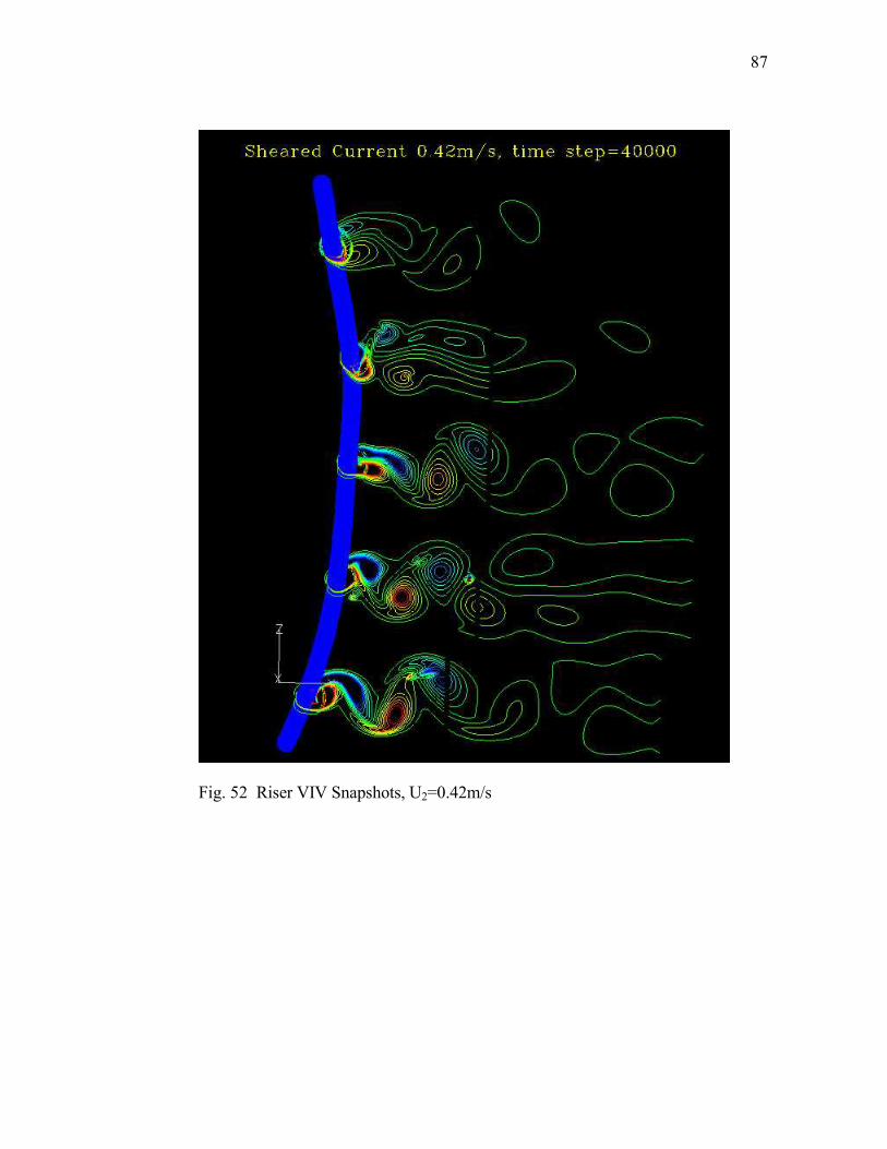
87
Fig. 52 Riser VIV Snapshots, U2=0.42m/s
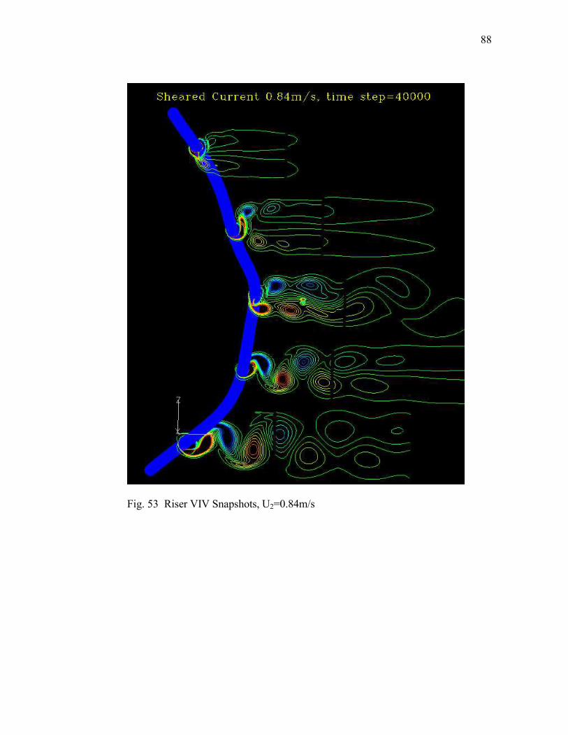
88
Fig. 53 Riser VIV Snapshots, U2=0.84m/s

89
Riser CF Response @ x/L=0.44
-1
-0.8
-0.6
-0.4
-0.2
0
0.2
0.4
0.6
0.8
1
6 7 8 9 10 11 12 13 14 15 16
t (sec)
z/D
FANS (U2=0.42m/s)
Experiment (U2=0.42m/s)
Fig. 54 Riser Cross Flow Response Time History (U2=0.42m/s)
Riser CF Response @ x/L=0.44
-1
-0.8
-0.6
-0.4
-0.2
0
0.2
0.4
0.6
0.8
1
4 4.5 5 5.5 6 6.5 7 7.5 8 8.5 9
t (sec)
z/D
FANS (U2=0.84m/s)
Experiment (U2=0.84m/s)
Fig. 55 Riser Cross Flow Response Time History (U2=0.84m/s)

90
CF Motion rms a/D (U2=0.42m/s)
0.00
0.10
0.20
0.30
0.40
0.50
0 0.2 0.4 0.6 0.8 1x/L
rms a/D
Test 1205
CFD (FANS)
Fig. 56 Riser Cross Flow Response rms a/D (U2=0.42m/s)
CF Motion rms a/D (U2=0.84m/s)
0.00
0.10
0.20
0.30
0.40
0.50
0 0.2 0.4 0.6 0.8 1x/L
rms a/D
Test 1210
CFD (FANS)
Fig. 57 Riser Cross Flow Response rms a/D (U2=0.84m/s)

91
CF Motion PSD (Test 1205, U2=0.42m/s)
0.0E+00
5.0E-04
1.0E-03
1.5E-03
2.0E-03
2.5E-03
3.0E-03
3.5E-03
4.0E-03
4.5E-03
0 20 40 60 80 100 120 140
w (rad/s)
CF Response PSD (m^2-s/rad)
Fig. 58 Riser Cross Flow Response PSD (Test 1205, U2=0.42m/s)
CF Motion PSD (FANS, U2=0.42m/s)
0.0E+00
5.0E-04
1.0E-03
1.5E-03
2.0E-03
2.5E-03
3.0E-03
3.5E-03
0 20 40 60 80 100 120 140w (rad/s)
CF Motion PSD (m^2-s/rad)
Fig. 59 Riser Cross Flow Response PSD (CFD, U2=0.42m/s)
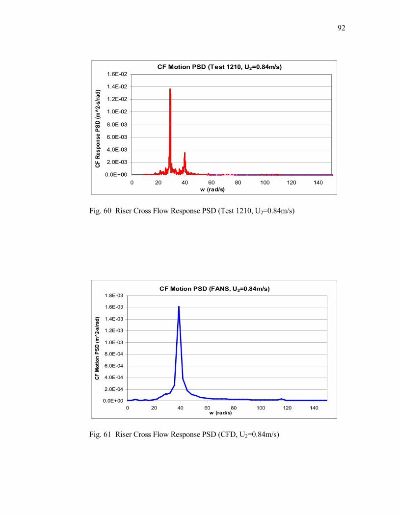
92
CF Motion PSD (Test 1210, U2=0.84m/s)
0.0E+00
2.0E-03
4.0E-03
6.0E-03
8.0E-03
1.0E-02
1.2E-02
1.4E-02
1.6E-02
0 20 40 60 80 100 120 140
w (rad/s)
CF Response PSD (m^2-s/rad)
Fig. 60 Riser Cross Flow Response PSD (Test 1210, U2=0.84m/s)
CF Motion PSD (FANS, U2=0.84m/s)
0.0E+00
2.0E-04
4.0E-04
6.0E-04
8.0E-04
1.0E-03
1.2E-03
1.4E-03
1.6E-03
1.8E-03
0 20 40 60 80 100 120 140w (rad/s)
CF M
otion PSD (m^2-s/rad)
Fig. 61 Riser Cross Flow Response PSD (CFD, U2=0.84m/s)

93
The CF VIV induced fatigue damage index along the riser was calculated and
compared to experimental results (from stain gages) in Figs. 62 and 63 for U2=0.42m/s
and U2=0.84m/s respectively. The comparisons show that the fatigue damages are
comparable between the CFD simulation and experiments. In general the CFD code
predicts slightly higher fatigue damage than the experiment. It is worthwhile to note that
both CFD simulations and experiments show that the fatigue damage distributions on the
riser are not symmetric along the axial direction. One possible reason is the involvement
of the non-dominant modes. The non-dominant modes themselves contribute very small
fatigue damages. However, when they are superimposed to the dominant mode, their
influence is amplified by approximately 3 times (for single slope S-N curve with m1=3),
hence is able to noticeably change the fatigue distributions. Overall, the CFD approach
provides satisfactory results. And the comparisons confirm the feasibility of fatigue
assessment using CFD time domain simulation approach.

94
Fatigue Damage Index Comparison (U2=0.42m/s)
1.E+00
1.E+01
1.E+02
1.E+03
1.E+04
1.E+05
1.E+06
0 0.1 0.2 0.3 0.4 0.5 0.6 0.7 0.8 0.9 1
x/L
Damage Index (
µεµε µεµε3Hz)
CFD
Test #1205
Fig. 62 CF Fatigue Damage Index Comparison (U2=0.42m/s)
Fatigue Damage Index Comparison (U2=0.84m/s)
1.E+00
1.E+01
1.E+02
1.E+03
1.E+04
1.E+05
1.E+06
1.E+07
0 0.1 0.2 0.3 0.4 0.5 0.6 0.7 0.8 0.9 1
x/L
Damage Index (
µε
µε
µεµε3Hz)
CFD
Test #1210
Fig. 63 CF Fatigue Damage Index Comparison (U2=0.84m/s)

95
Discussions
In this chapter we have simulated a vertical riser VIV response in shear currents,
and compared to the experimental data. The riser has aspect ratio L/D of 482. The fluid-
riser interactions are computed and visualized in time domain. Based on that we
calculated the cross flow VIV induced stress and fatigue damage index, and compared
the fatigue results to experimental results. Some of the findings from the study are:
1. The CFD simulations of riser VIV show similar response as the experimental
data. We compared the important parameters, including motion time
histories, rms a/D, and PSDs. General agreements have been observed. The
CFD approach could slightly over-predict the response amplitudes.
2. Linearly shear current with higher speed tends to excite more modes. The
dominant mode contributes most to the VIV induced fatigue, while the non-
dominant modes could also influence the fatigue damage considerably by
enhancing or canceling the peak values. Both CFD simulation and
experiments show non-symmetric fatigue damage distributions along the
riser.
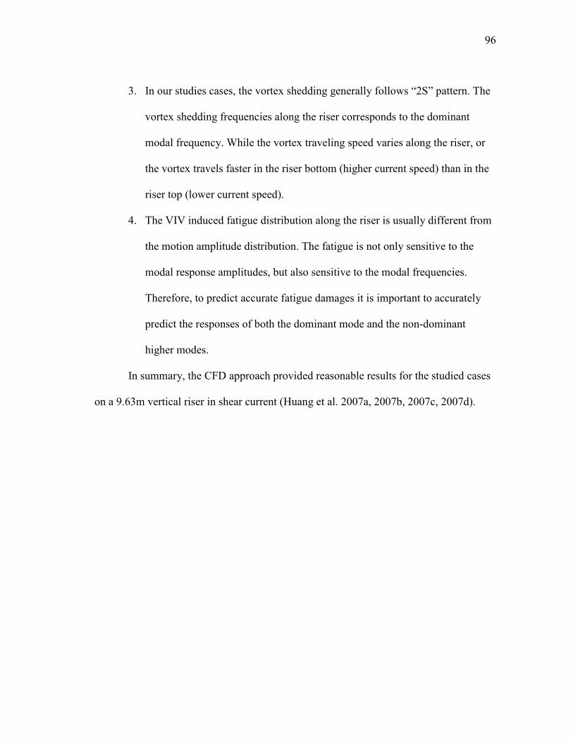
96
3. In our studies cases, the vortex shedding generally follows “2S” pattern. The
vortex shedding frequencies along the riser corresponds to the dominant
modal frequency. While the vortex traveling speed varies along the riser, or
the vortex travels faster in the riser bottom (higher current speed) than in the
riser top (lower current speed).
4. The VIV induced fatigue distribution along the riser is usually different from
the motion amplitude distribution. The fatigue is not only sensitive to the
modal response amplitudes, but also sensitive to the modal frequencies.
Therefore, to predict accurate fatigue damages it is important to accurately
predict the responses of both the dominant mode and the non-dominant
higher modes.
In summary, the CFD approach provided reasonable results for the studied cases
on a 9.63m vertical riser in shear current (Huang et al. 2007a, 2007b, 2007c, 2007d).

97
CHAPTER VI
3D SIMULATION OF FLOW PAST A HORIZONTAL RISER
IN UNIFORM CURRENT
This chapter presents the study results on a horizontal riser (L/D=1,400), which
was the subject of a recently experiment conducted at Marintek’s Ocean Basin in
Trondheim (Trim et al. 2005). Fig. 64 shows the testing schematics plan view. The riser
model has a mass ratio of 1.6, and length of 38 m. It is towed through the wave basin to
generate desired current conditions. The testing was performed under different the
current conditions, i.e. uniform and shear current. Some experimental data are published
in Trim’s paper (2005).
U
U
riser
water basin
L=38m
φ=0.027m
m*=1.6
Fig. 64 Riser VIV Testing Plan View Schematics

98
In this chapter we intended to further demonstrate that the long riser VIV could
also be analyzed by using Chimera (overset grid) technique embedded CFD approach.
The studied riser is positioned horizontally with uniform sectional properties and
constant tension. Its two ends have pinned connection boundary conditions. In such case
its modal shapes follow sinusoidal functions and are well defined by simple analytic
formula. A uniform current of 0.4 m/s and 0.8 m/s are applied to the riser respectively,
the riser response is then calculated in time domain for sufficiently long durations. The
simulation results are compared to the published experimental data and CFD results.
The flow field around a riser is calculated by numerically solving the unsteady,
incompressible Navier-Stokes equation. The turbulence flow was solved using Large
Eddy Simulation (LES) with Smagorinsky subgrid-scale turbulence model. The
Reynolds numbers are 8x10³ and 1.7x10
4 for U=0.4 m/s and U=0.8 m/s respectively.
The non-dimensional time step used in the simulation is 0.01, which means the
free stream fluid travels a distance of one riser diameter in 100 time steps. The
dimensional time steps are about 0.0007 seconds for U=0.4 m/s current, and half of that
for U=0.8 m/s current. Considering that both the vortex shedding frequency for the fixed
riser and the vibrating frequency of the riser are less than 3 Hz, this time step is
sufficiently small.

99
Overset grid (Chimera) technique provides an effective way to handle riser
movement. Figs. 65 and 66 show the structured data grids used in this study. The body
grid has a dimension of 182 x 41 x 30, the wake grid has a dimension of 200 x 101 x 30,
while the background grid is artificial. It provides boundary conditions to the wake grid,
but does not involve in numerical iterations. Therefore, it is not shown in the figures.
The data grids have a total of slightly less than 1 million elements, and have been
delicately generated with very fine grid sizes at the riser boundary layer and vortex
shedding zones. In this study the wake grid is set to move with the riser, which
eliminates the relative movement between the riser body grid and wake grid. As a result,
the overlapping region depends on only the riser initial position, and the interpolation
coefficients between these two grids needs only to be determined once throughout the
simulation. Fig. 65 illustrates the data grids when riser is at its initial position (not
deflected) and deformed due to current loadings. Fig. 66 shows the grid details
around/along the riser surface.
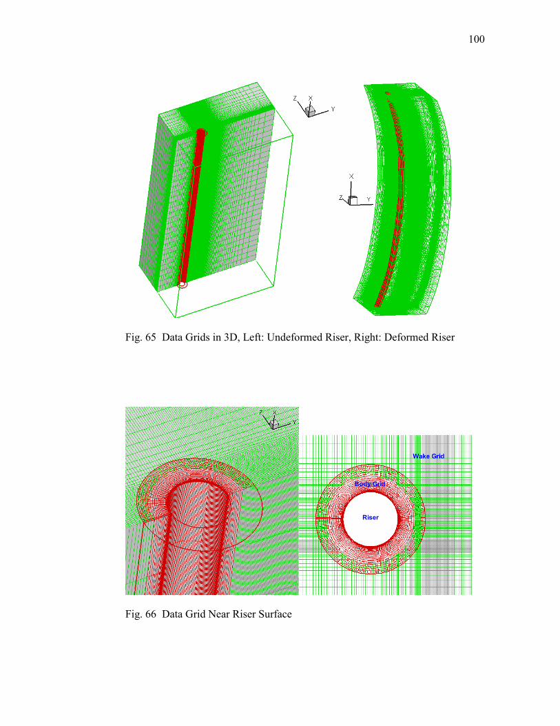
100
Fig. 65 Data Grids in 3D, Left: Undeformed Riser, Right: Deformed Riser
Wake Grid
Body Grid
Riser
Fig. 66 Data Grid Near Riser Surface

101
The simulation starts with an initial uniform flow on the background data grid.
The riser deflects toward the current direction until its internal restoring force overcomes
the current drag force. After a certain period of transitional dynamics, it then oscillates
about its equilibrium position. The riser motions were solved using the modal solver.
Both inline and cross flow motions are included in this study.
Simulation Results
We started the riser VIV simulation with an initially straight riser. Because it is
subject to the mean drag force, the riser deflects toward the downstream direction. The
maximum riser deflections occur at the middle section, with values of approximately 5D
and 20D for current speed 0.4 m/s and 0.8 m/s respectively. Fig. 67 shows the evolution
of this deflection and the vorticity of the flowing field around the riser. The results
indicate that the riser approaches near its equilibrium position after 6,000 time steps
(current travels a distance of 60D), and its inline vibrating amplitudes are small
comparing to the riser mean deflections. The figure also shows the vortex shedding at
different locations along the riser can be either in phase or our-of-phase. Majority of the
vortex shedding show clear 2S pattern. Occasionally coalescence of vortex (C pattern)
occurs near top and bottom regions. This indicates that the riser is self-exciting most of
the time throughout the whole riser span.
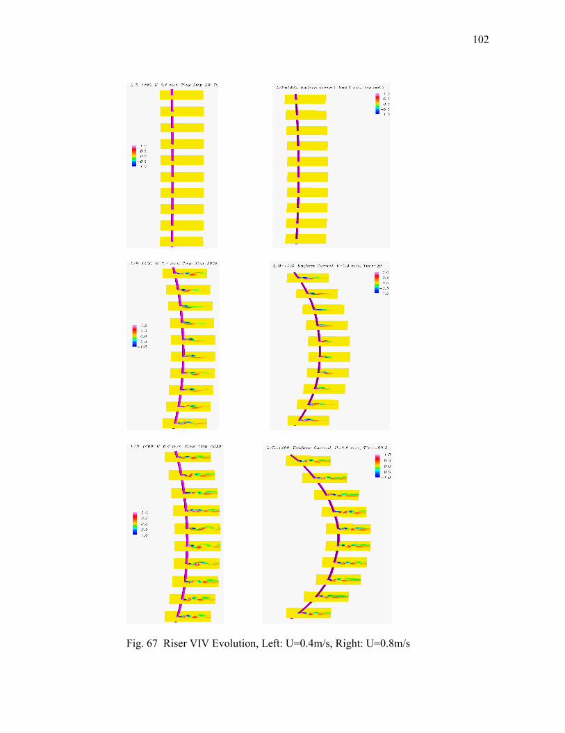
102
Fig. 67 Riser VIV Evolution, Left: U=0.4m/s, Right: U=0.8m/s

103
Figs. 68 and 69 present the riser and flow field vorticity contour snap shots for
U=0.4 m/s and 0.8 m/s respectively. Only 5 sectional planes are shown. It confirms that
the vortex shedding at different riser sectional stations are synchronized with the riser
motions. Furthermore, it also illustrates the riser VIV response in 3D, including in-line
and cross flow vibrations. It is interesting to see the large riser mean deflections in flow
direction. We noticed that this in-line deflection could affect the riser VIV responses,
both in-line VIV and cross flow VIV. To illustrate this, we plotted the 1st mode response
time histories in Figs. 70 and 71 for U=0.4 m/s and 0.8 m/s respectively. It shows that:
• The 1st mode amplitude approaches a large mean value, i.e. 5.2D for U=0.4
m/s, and 23.3D for U=0.8 m/s. Note that the mean value increases by
approximately 4 times when current velocity doubles, which is as expected
since the current loading is proportional to the square of the speed. Also note
that the 1st mode response is different from the riser response. The former is
only a component of the later.
• The 1st mode amplitude decays very slowly, if it decays at all. It oscillates
about its mean value with a standard deviation of 0.4D and 1D for U=0.4 m/s
and 0.8 m/s respectively. Therefore, it seems the 1st mode dynamics is
intrinsic and somewhat proportional to the incoming current speed. These
standard deviations are in the same order of magnitude with the riser
diameter, and obviously comparable to the in-line and cross flow VIV
amplitudes.
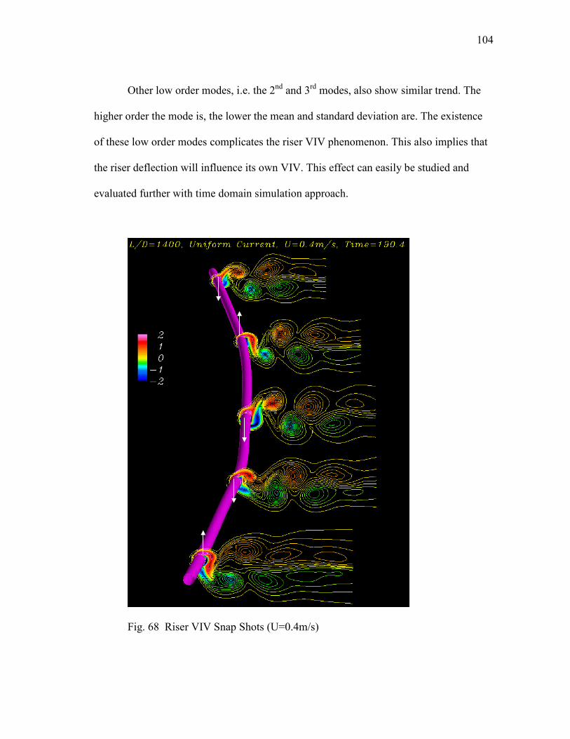
104
Other low order modes, i.e. the 2nd and 3
rd modes, also show similar trend. The
higher order the mode is, the lower the mean and standard deviation are. The existence
of these low order modes complicates the riser VIV phenomenon. This also implies that
the riser deflection will influence its own VIV. This effect can easily be studied and
evaluated further with time domain simulation approach.
Fig. 68 Riser VIV Snap Shots (U=0.4m/s)
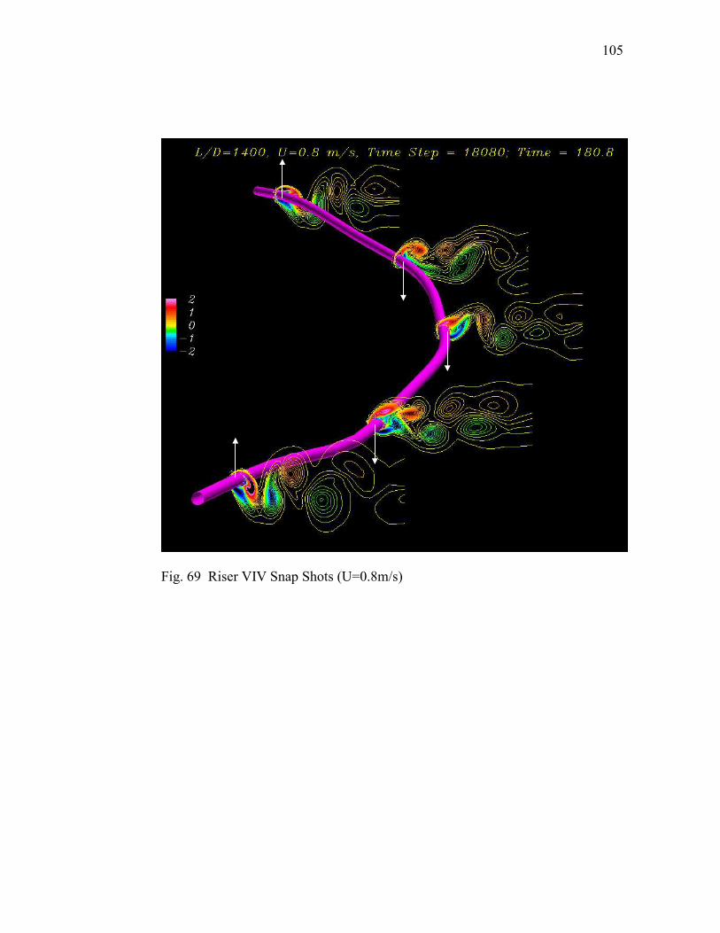
105
Fig. 69 Riser VIV Snap Shots (U=0.8m/s)

106
0
1
2
3
4
5
6
7
0 5000 10000 15000 20000
Time Step
Y/D
1st Mode Amplitude
Mean/D=5.2
stdev/D=0.4
Fig. 70 In-Line Modal Response (U=0.4m/s)
0
5
10
15
20
25
30
0 5000 10000 15000 20000
Time Step
Y/D
1st Mode Amplitude
Mean/D=23.3
stdev/D=1.0
Fig. 71 In-Line Modal Response (U=0.8m/s)
Drag and lift coefficients are calculated at each time step along the riser. Fig. 72
shows the mean drag coefficient distributions. The drag coefficients are calculated based
on global current velocity and have mean values between 1 and 2.5. By comparing the
mean Cd distributions to the riser cross flow VIV amplitude envelopes (shown in page
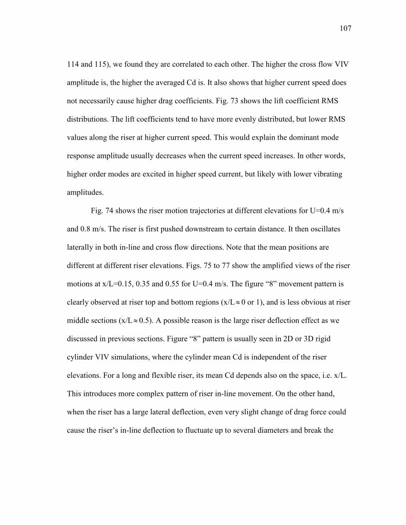
107
114 and 115), we found they are correlated to each other. The higher the cross flow VIV
amplitude is, the higher the averaged Cd is. It also shows that higher current speed does
not necessarily cause higher drag coefficients. Fig. 73 shows the lift coefficient RMS
distributions. The lift coefficients tend to have more evenly distributed, but lower RMS
values along the riser at higher current speed. This would explain the dominant mode
response amplitude usually decreases when the current speed increases. In other words,
higher order modes are excited in higher speed current, but likely with lower vibrating
amplitudes.
Fig. 74 shows the riser motion trajectories at different elevations for U=0.4 m/s
and 0.8 m/s. The riser is first pushed downstream to certain distance. It then oscillates
laterally in both in-line and cross flow directions. Note that the mean positions are
different at different riser elevations. Figs. 75 to 77 show the amplified views of the riser
motions at x/L=0.15, 0.35 and 0.55 for U=0.4 m/s. The figure “8” movement pattern is
clearly observed at riser top and bottom regions (x/L≈0 or 1), and is less obvious at riser
middle sections (x/L≈0.5). A possible reason is the large riser deflection effect as we
discussed in previous sections. Figure “8” pattern is usually seen in 2D or 3D rigid
cylinder VIV simulations, where the cylinder mean Cd is independent of the riser
elevations. For a long and flexible riser, its mean Cd depends also on the space, i.e. x/L.
This introduces more complex pattern of riser in-line movement. On the other hand,
when the riser has a large lateral deflection, even very slight change of drag force could
cause the riser’s in-line deflection to fluctuate up to several diameters and break the
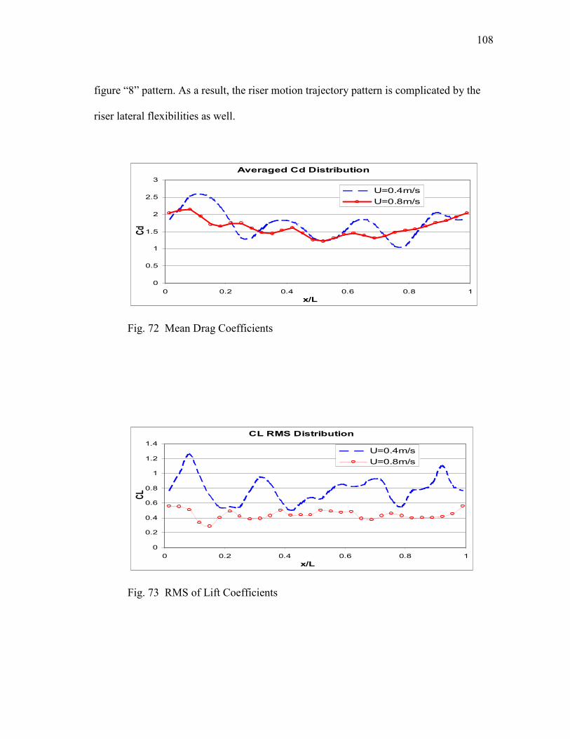
108
figure “8” pattern. As a result, the riser motion trajectory pattern is complicated by the
riser lateral flexibilities as well.
Averaged Cd Distribution
0
0.5
1
1.5
2
2.5
3
0 0.2 0.4 0.6 0.8 1
x/L
Cd
U=0.4m/s
U=0.8m/s
Fig. 72 Mean Drag Coefficients
CL RMS Distribution
0
0.2
0.4
0.6
0.8
1
1.2
1.4
0 0.2 0.4 0.6 0.8 1
x/L
CL
U=0.4m/s
U=0.8m/s
Fig. 73 RMS of Lift Coefficients

109
-1.5
-1
-0.5
0
0.5
1
1.5
0 1 2 3 4 5 6 7
y/D
z/D
x/L=0.15
-1.5
-1
-0.5
0
0.5
1
1.5
0 5 10 15 20 25
y/D
z/D
x/L=0.15
-1.5
-1
-0.5
0
0.5
1
1.5
2
0 1 2 3 4 5 6 7
y/D
z/D
x/L=0.35
-1.5
-1
-0.5
0
0.5
1
1.5
0 5 10 15 20 25
y/D
z/D
x/L=0.35
-1
-0.5
0
0.5
1
1.5
0 1 2 3 4 5 6 7
y/D
z/D
x/L=0.55
-1.5
-1
-0.5
0
0.5
1
1.5
0 5 10 15 20 25
y/D
z/D
x/L=0.55
-1.5
-1
-0.5
0
0.5
1
1.5
2
0 1 2 3 4 5 6 7
y/D
z/D
x/L=0.75
-1.5
-1
-0.5
0
0.5
1
1.5
0 5 10 15 20 25
y/D
z/D
x/L=0.75
Fig. 74 Riser Motion Trajectory, Left: U=0.4m/s, Right:U=0.8m/s

110
-1.5
-1
-0.5
0
0.5
1
1.5
2 2.5 3 3.5
y/D
z/D
x/L=0.15
Fig. 75 Riser Motion Trajectory at x/L=0.25, U=0.4m/s
-1.5
-1
-0.5
0
0.5
1
1.5
3.5 4 4.5 5 5.5
y/D
z/D
x/L=0.35
Fig. 76 Riser Motion Trajectory at x/L=0.35, U=0.4m/s
-1.5
-1
-0.5
0
0.5
1
4 4.5 5 5.5 6
y/D
z/D
x/L=0.55
Fig. 77 Riser Motion Trajectory at x/L=0.55, U=0.4m/s
111
To investigate into more details on the riser VIV, we plotted the riser cross flow
motion snap shots in Figs. 78 and 79. It shows the envelope of the dominant mode. The
responses are not exactly symmetric. This could be due to the interference from the low-
mode riser vibrations in both the in-line and cross flow direction, as we discussed later in
this section. We also plotted the riser motion RMS a/D in Figs. 80 to 83, and compared
the results to the experimental data (Trim et al. 2005) and published CFD results
(Holmes et al. 2006). Generally the comparisons show very good agreement to the
experimental data. Some highlights are:
• For cross flow VIV the dominant modes are clear: FANS predicted the 4th
mode is dominant for U=0.4 m/s and the 6th mode is dominant for U=0.8 m/s.
The model testing shows the 3rd mode is dominant for U=0.4 m/s. One
possible reason would be the tension variation. In our calculation the tension
within the riser is set to 5 kN, while in the model testing it varies in a range
from 4 kN to 6 kN.
• For in-line VIV the dominant modes are not obvious in FANS’ results.
However, the model testing shows the 5th mode is dominant for U=0.4 m/s.
Again this is likely due to the lower order mode dynamics. We suspect that in
the model testing the gravity of the riser has played a role in the riser in-line
VIV by acting as a restoring force. Further assessment is needed to confirm
that.
The maximum cross flow rms a/D is also compared to the experimental data at
U=0.4 m/s and 0.8 m/s in Fig. 84. It shows good agreement as well. We noticed that the

112
locations of the maximum riser response are not at the riser middle section. Some of
them are near the two ends of the riser. This could be due to the “pinned” boundary
conditions, where all the modes have zero curvature at the two ends, and the peak
curvature values of the excited modes are most likely to add together near the ends.
Another interesting phenomenon is that the cross flow VIV is not symmetric
along the riser. This is clearly shown in the experimental data: the rms has a trend of
going higher at large x/L. We also found the same in our results. Further investigations
disclose that the 2nd in-line mode (and higher even order modes) excitation could be the
reason. We plotted the in-line motion time histories at x/L=0.25 and 0.75, take the
difference between these two motions, and compare that to the 2nd in-line mode
amplitude, as shown in Fig. 85. The correlation between these two is obvious. Due to the
existence of the even order in-line mode, the riser top and bottom section experience
different relative fluid-riser velocities, hence different lift forces.
-1
-0.8
-0.6
-0.4
-0.2
0
0.2
0.4
0.6
0.8
1
0 200 400 600 800 1000 1200 1400
X/D
Y/D
Fig. 78 Riser CF Response Envelope for U=0.4m/s, t=193~200

113
-1.4
-1.2
-1
-0.8
-0.6
-0.4
-0.2
0
0.2
0.4
0.6
0.8
0 200 400 600 800 1000 1200 1400
X/D
Y/D
Fig. 79 Riser CF Response Envelope for U=0.8m/s, t=193~200
IL Motion RMS (U=0.4m/s)
0
0.05
0.1
0.15
0.2
0.25
0 0.2 0.4 0.6 0.8 1
x/L
rms a/D
FANS (CFD)
Trim et al. (experiment)Holmes et al. (CFD)
Fig. 80 Riser In Line VIV RMS for U=0.4m/s

114
CF Motion RMS (U=0.4m/s)
0
0.1
0.2
0.3
0.4
0.5
0.6
0.7
0 0.2 0.4 0.6 0.8 1
x/L
rms a/D
FANS (CFD)Trim et al. (experiment)Holmes et al. (CFD)
Fig. 81 Riser Cross Flow VIV RMS for U=0.4m/s
IL Motion RMS (U=0.8m/s)
0
0.05
0.1
0.15
0.2
0.25
0.3
0.35
0 0.2 0.4 0.6 0.8 1
x/L
rms a/D
FANS (CFD)
Holmes et al. (CFD)
Fig. 82 Riser In Line VIV RMS for U=0.8m/s

115
CF Motion RMS (U=0.8m/s)
0
0.1
0.2
0.3
0.4
0.5
0.6
0.7
0.8
0 0.2 0.4 0.6 0.8 1
x/L
rms a/D
FANS (CFD)Trim et al. (experiment)Holmes et al. (CFD)
Fig. 83 Riser Cross Flow VIV RMS for U=0.8m/s
Max CF RMS a/D
0
0.2
0.4
0.6
0.8
1
1.2
0 0.5 1 1.5 2 2.5
U (m/s)
CF M
ax RMS a/D
FANS (CFD)
Trim et al. (experiment)
Holmes et al. (CFD)
Fig. 84 Riser Cross Flow VIV Max RMS
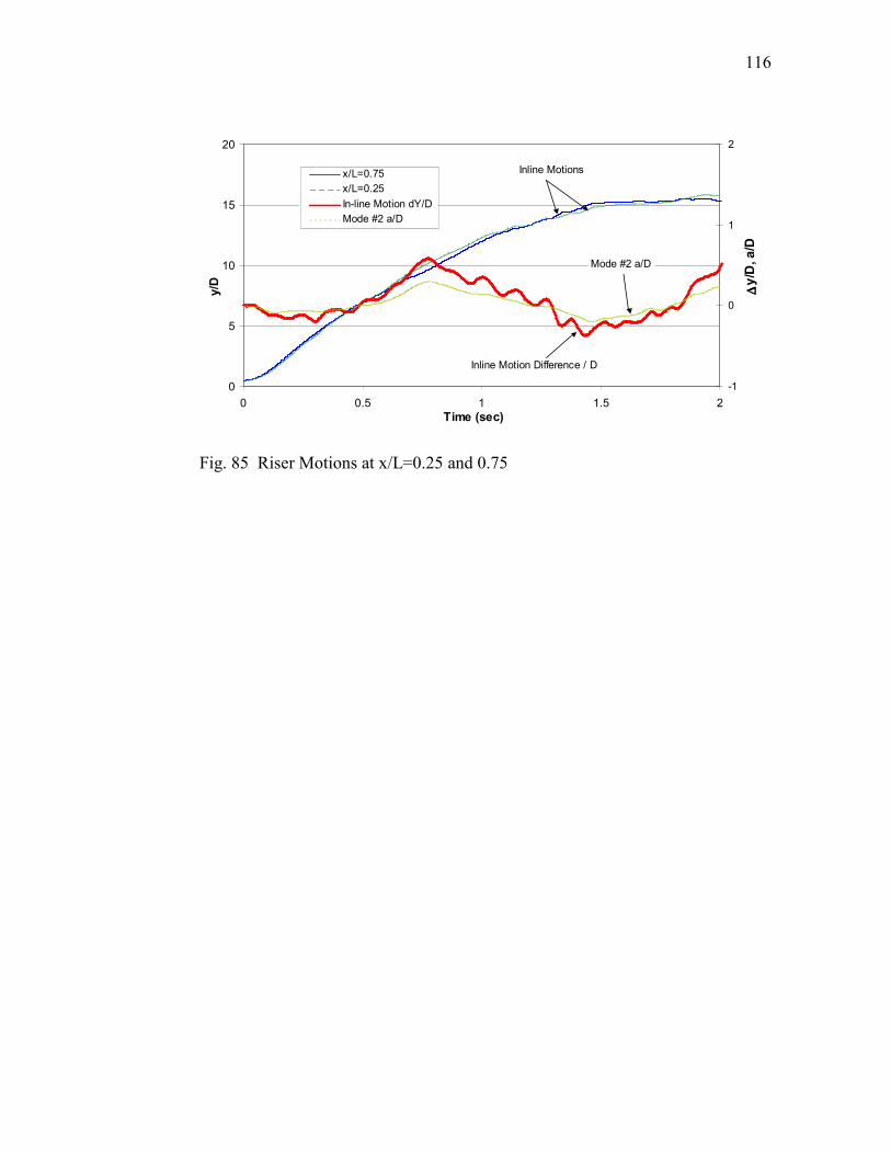
116
0
5
10
15
20
0 0.5 1 1.5 2
Time (sec)
y/D
-1
0
1
2
ΔΔ ΔΔy/D, a/D
x/L=0.75
x/L=0.25
In-line Motion dY/D
Mode #2 a/D
Inline Motions
Inline Motion Difference / D
Mode #2 a/D
Fig. 85 Riser Motions at x/L=0.25 and 0.75

117
Discussions
This chapter studied a long riser VIV response by using an unsteady, overset-grid
(Chimera), Navier-Stokes method. We presented two case studies with uniform current
speed of 0.4 m/s and 0.8 m/s respectively. The total element number used for the
computation of fluid domain is less than 1 million. And the results are in good
agreement with published experimental data. It is found that when constrained by data
grid element number, it is more efficient to focus on accurate prediction of drag and lift
forces than the flow details in spanwise direction. Nevertheless, more elements could be
used in the riser axial direction to provide better resolution, hence more accurate drag
and lift force distributions. For deepwater risers, when current speed is high, very high
order modes could be excited. Therefore, the data grid in riser spanwise direction should
be adequately fine to predict the high order VIV response with acceptable accuracy.
In this study it also demonstrated that the time domain CFD approach is able to
provide more valuable details on the drag force, lift force, fluid velocities and vorticities,
riser displacement and modal response time histories. We successfully used FANS to
illustrate some of the interesting but not explained phenomena in the experimental data.
In conclusion, a CFD approach that could be applied to long marine riser VIV
assessment has been presented. And its validity and effectiveness to predict long riser
VIV in uniform current have been demonstrated through case studies and comparisons to
published experimental data (Huang et al. 2007a, 2007b, 2007c, 2007d).
118
CHAPTER VII
3D SIMULATION OF FLOW PAST A HORIZONTAL RISER
IN SHEAR CURRENT
In Chapter XII we compared the VIV simulation results of a long riser
(L/D=1,400) to the experimental data in uniform currents. In this chapter we continue to
use the same CFD approach and data grids to study the riser VIV response in shear
current. In order to facilitate a direct comparison with the experimental data of Trim et
al. (2005), we have chosen two linearly shear current profiles with maximum speeds of
0.4 m/s and 0.8 m/s respectively. During the experiment, the riser was horizontally
positioned under the water. One end of the riser was fixed, while the other end was
towed in circular movement at constant speed. This would simulate a linearly shear
current. The effect on VIV due to the riser circular movement is expected to be small, as
discussed in Holmes et al. (2006).
The riser is 38 m in length and 0.027 m in diameter. In the simulations, the drag
(Cd) and lift (CL) coefficients are calculated along the riser at each time step. Then the
riser motions are solved by a modal motion solver as if the drag and lift forces are
constant. This is an explicit approach without iteration between the flow field and the
riser motion. We used the 4th order Runge-Kutta method to integrate the motion
equation. The riser was modeled as a beam with a constant tension of 5 kN. Its two ends
are assumed to have pinned connections. No damping has been included. It is estimated
that the dominant mode should be less than the 10th mode. Therefore, the riser bending

119
stiffness was expected to have very limited effect on the results, and was neglected in
this study. The Reynolds number varies along the riser. It has a maximum value of
1.7x10⁵ at x/L = 1.0 for Umax=0.8 m/s case.
Simulation Results
The riser VIV responses in two linearly shear current profiles are analyzed.
These two profiles are illustrated in Fig. 86. We chose these two current profiles to
facilitate a direct comparison of the simulation results with the experiment data and other
numerical investigations.
Umax=0.4m/s
0
0.25
0.5
0.75
1
0 0.2 0.4 0.6 0.8
V (m/s)
x/L
Umax=0.8m/s
0
0.25
0.5
0.75
1
0 0.2 0.4 0.6 0.8
V (m/s)
x/L
Fig. 86 Linearly Shear Currents
120
The simulations started with an initially un-deformed riser. The riser begins to
move after it is subjected to a shear current, and deflects continuously until its internal
restoring force is sufficiently large to overcome the drag forces. Theoretically, this
motion is transient and subsides as simulation continues. However, we found that the
transient response decays rather slowly over the duration of the present simulations,
which made it difficult to distinguish this transient motion from the riser in-line VIV.
The time domain simulations are carried out to a total of 20,000 time steps, or
fluid travels a total distance of 200 OD (5.4 m) at x/L=1 for Umax=0.4 m/s case. Fig. 87
shows the evolution of the riser VIV and vortex shedding under different current
profiles. The left hand side riser is undergoing VIV in shear current, while the right hand
side riser is undergoing VIV in uniform current. Both risers start with un-deformed
configuration. After a period (approximately 4,000 time steps) of transient response,
both risers reach nearly equilibrium positions. The maximum riser deflection occurs at
the middle section for risers in uniform current, while it occurs at a slightly higher
position in the shear current. The maximum riser deflection amplitude in the uniform
current is approximately four times of that in the shear current. This is reasonable since
the averaged speed for the shear current is half of that for the uniform current, and the
drag force is proportional to the square of the current speed. Majority of the vortex
shedding shows a clear 2S pattern, which is defined in Williamson and Roshko (1988).
Coalescence of vortex (C pattern) also exists in both cases. It occurs near the top and
bottom regions in the uniform current, and around the middle section in the shear
121
current. The cross flow VIV amplitudes are moderate and in the order of 1D. No obvious
2T patterns (Williamson and Jauvtis, 2004) have been observed in these two-degree-of-
freedom simulations.
Fig. 88 shows two snap shots of the vorticity fields for Umax=0.4 m/s and
Umax=0.8 m/s respectively. The riser maximum lateral deflection for Umax=0.8 m/s
case is approximately 5~6 times of the riser diameter. As expected, it is much larger than
that of the Umax=0.4 m/s case. It is also observed in both cases that the 2S pattern and C
pattern are mixed along the riser. The C pattern indicates a possible power out region.
Therefore, it is likely that the riser middle section is the power in region, while the riser
top and bottom sections are the power out regions (Vandiver and Li, 2003).
Fig. 89 shows the vorticity contours for Umax=0.4m/s and Umax=0.8m/s,
respectively, at selected time instants. For Umax=0.8m/s case, the dominant modal shape
number (7th mode) is much higher than that (3
rd mode) of the Umax=0.4 m/s case.

122
Fig. 87 Vortex Shedding, Umax=0.4m/s, Left: Shear, Right: Uniform

123
Fig. 88 Riser VIV Snap Shots, Left: Umax=0.4m/s, Right: Umax=0.8m/s
Fig. 89 Vorticity Contours, Left: Umax=0.4m/s, Right: Umax=0.8m/s

124
The drag and lift coefficients are calculated at each time step. Figs. 90 to 93 show
the comparisons between the uniform and the shear current cases. It shows that the drag
coefficients are in the similar ranges for all cases, with minor variations due to different
dominant modes. While the lift coefficients for shear current are generally lower than
those for the uniform current. This could be related to the riser vibration mode dominant
level and amplitudes in these two current profiles. It is not surprising to see that the
single mode dominant is more likely to occur in uniform current than in shear current,
and with higher a/D rms values. The lift coefficients also show variations along the riser
that corresponds to the dominant mode shapes. The higher the current speed, the higher
the dominant mode number becomes. Hence more peaks and troughs are observed in the
lift coefficients for U = 0.8 m/s case. The results also show that the lift coefficients have
a rms value of 0.2~0.4 in shear current profiles. The averaged values for shear current
cases are 0.34 for Umax = 0.4 m/s, and 0.32 for Umax = 0.8 m/s. On the other hand, the
averaged rms values are 0.78 for U=0.4 m/s and 0.44 for U=0.8 m/s in the uniform
current cases. Although the exact values are case dependent, it seems that the lift
coefficients are less sensitive to the current speed under shear current condition. The
drag coefficients are slightly higher at the riser top and bottom regions in uniform
current cases. One possible reason could be due to the vortex shedding pattern near the
top and bottom boundaries (C pattern). Note that the mean drag coefficient is related to
several factors, including Reynolds number, riser vibrating amplitudes and frequencies.
Therefore, high velocity does not necessarily result in high drag coefficient, as shown in
the shear current cases.

125
Averaged Cd Distribution (U=0.4m/s)
0
0.5
1
1.5
2
2.5
3
0 0.2 0.4 0.6 0.8 1
x/L
Cd
Uniform Current
Sheared Current
Fig. 90 Drag Coefficient Distribution, Umax=0.4m/s
CL RMS Distribution (U=0.4m/s)
0
0.2
0.4
0.6
0.8
1
1.2
1.4
0 0.2 0.4 0.6 0.8 1
x/L
CL
Uniform Current
Sheared Current
Fig. 91 Lift Coefficient Distribution, Umax=0.4m/s
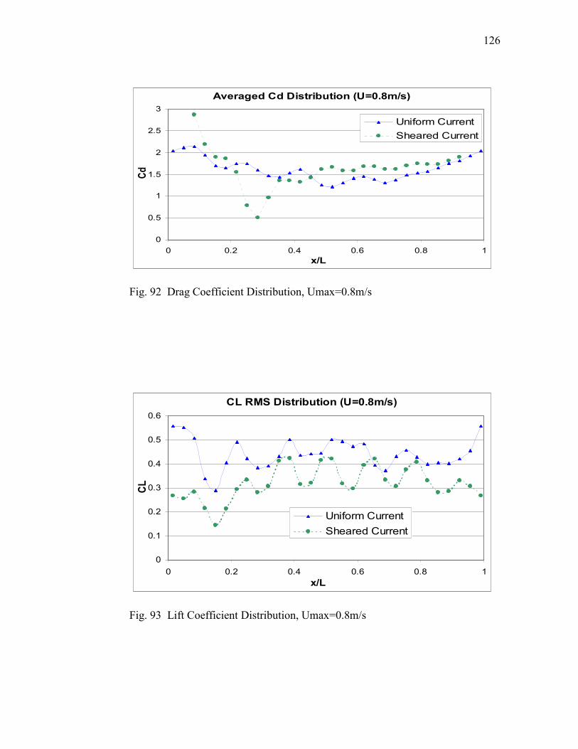
126
Averaged Cd Distribution (U=0.8m/s)
0
0.5
1
1.5
2
2.5
3
0 0.2 0.4 0.6 0.8 1
x/L
Cd
Uniform Current
Sheared Current
Fig. 92 Drag Coefficient Distribution, Umax=0.8m/s
CL RMS Distribution (U=0.8m/s)
0
0.1
0.2
0.3
0.4
0.5
0.6
0 0.2 0.4 0.6 0.8 1
x/L
CL
Uniform Current
Sheared Current
Fig. 93 Lift Coefficient Distribution, Umax=0.8m/s

127
The riser response rms a/D is of particular interest in the riser VIV simulations.
Figs. 94 and 96 show the comparison between the simulation results and experiment data
in cross flow VIV. The experimental data are plotted in straight lines since only the
mean and maximum values are given in the experiment of Trim et al. (2005). Our CFD
simulation results predicted similar maximum and mean values as the experiment data
for the slower shear current case (Umax=0.4 m/s), while under-predicted the VIV in
higher shear current case (Umax=0.8 m/s). Fig. 96 shows the comparison of maximum
rms a/D. In general the CFD approach tends to underestimate the riser VIV peak
response. The in-line riser VIV rms a/D is not presented since it is dominated by the
transient motions as noted in earlier discussions. Hence, it is difficult to distinguish the
in-line VIV from the overall dynamic motions.
For completeness, the riser motion trajectories for both the shear and uniform
currents are also shown in Figs. 97 and 98 for Umax = 0.4 m/s and 0.8 m/s cases,
respectively. The figure “8” pattern is clearly shown only when the in-line motion is
small, and the dominant mode number is low, i.e. x/L=0.15 and Umax=0.4 m/s.
Otherwise, the riser movement does not necessarily take any simple shapes.

128
CF Motion RMS
0
0.05
0.1
0.15
0.2
0.25
0.3
0.35
0.4
0 0.2 0.4 0.6 0.8 1
x/L
rms a/D
U=0.4m/s, (FANS)
U=0.4m/s, max (Trim et al.)
U=0.4m/s, mean (Trim et al.)
Fig. 94 Cross Flow VIV RMS a/D, Umax=0.4m/s
CF Motion RMS
0
0.05
0.1
0.15
0.2
0.25
0.3
0.35
0.4
0.45
0.5
0 0.2 0.4 0.6 0.8 1
x/L
rms a/D
U=0.8m/s, (FANS)
U=0.8m/s, max (Trim et al.)
U=0.8m/s, mean (Trim et al.)
Fig. 95 Cross Flow VIV RMS a/D, Umax=0.8m/s

129
Max CF RMS a/D
0
0.1
0.2
0.3
0.4
0.5
0.6
0.7
0.8
0 0.5 1 1.5 2 2.5
U (m/s)
CF M
ax RMS a/D
FANS (CFD)
Trim et al. (experiment)
Holmes et al. (CFD)
Fig. 96 Cross Flow VIV Max RMS a/D
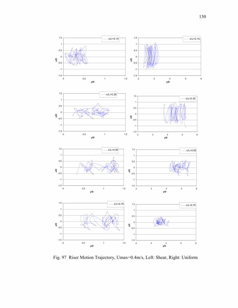
130
-1.5
-1
-0.5
0
0.5
1
1.5
0 0.5 1 1.5
y/D
z/D
x/L=0.15
-1.5
-1
-0.5
0
0.5
1
1.5
2 3 4 5 6
y/D
z/D
x/L=0.15
-1.5
-1
-0.5
0
0.5
1
1.5
0 0.5 1 1.5
y/D
z/D
x/L=0.35
-1.5
-1
-0.5
0
0.5
1
1.5
2 3 4 5 6
y/D
z/D
x/L=0.35
-1.5
-1
-0.5
0
0.5
1
1.5
0 0.5 1 1.5
y/D
z/D
x/L=0.55
-1.5
-1
-0.5
0
0.5
1
1.5
2 3 4 5 6
y/D
z/D
x/L=0.55
-1.5
-1
-0.5
0
0.5
1
1.5
0 0.5 1 1.5
y/D
z/D
x/L=0.75
-1.5
-1
-0.5
0
0.5
1
1.5
2 3 4 5 6
y/D
z/D
x/L=0.75
Fig. 97 Riser Motion Trajectory, Umax=0.4m/s, Left: Shear, Right: Uniform

131
-1.5
-1
-0.5
0
0.5
1
1.5
1 2 3 4 5 6 7 8
y/D
z/D
x/L=0.15
-1.5
-1
-0.5
0
0.5
1
1.5
10 12 14 16 18 20 22 24
y/D
z/D
x/L=0.15
-1.5
-1
-0.5
0
0.5
1
1.5
1 2 3 4 5 6 7 8
y/D
z/D
x/L=0.35
-1.5
-1
-0.5
0
0.5
1
1.5
10 12 14 16 18 20 22 24
y/D
z/D
x/L=0.35
-1.5
-1
-0.5
0
0.5
1
1.5
1 2 3 4 5 6 7 8
y/D
z/D
x/L=0.55
-1.5
-1
-0.5
0
0.5
1
1.5
10 12 14 16 18 20 22 24
y/D
z/D
x/L=0.55
-1.5
-1
-0.5
0
0.5
1
1.5
1 2 3 4 5 6 7 8
y/D
z/D
x/L=0.75
-1.5
-1
-0.5
0
0.5
1
1.5
10 12 14 16 18 20 22 24
y/D
z/D
x/L=0.75
Fig. 98 Riser Motion Trajectory, Umax=0.8m/s, Left: Shear, Right: Uniform

132
The riser in-line and cross flow motion responses are calculated through modal
superposition. The rms a/D of each modal component are plotted in Figs. 99 and 100 for
in-line and cross flow respectively. The response includes both the riser transient
dynamic motions due to its initial positions and velocities, and the steady VIV. The
transient response is usually low frequency and low modes, as shown in Fig. 99. We
didn’t attempt to split the transient response and steady VIV in this section. Further
investigation is needed in order to separate the transient response from the steady VIV.
In order to measure the dominant level of an excited modal shape, we normalized
the modal energy by the total response energy. In other words, we looked at the modal
energy percentage of each mode. Fig. 101 shows the results for in-line motions, which is
dominated by the 1st mode. As discussed earlier, this 1
st mode is mainly due to the
transient effect. Fig. 102 shows the modal energy percentages of cross flow motions. For
each studied case, there is a single mode that contributes at least 40% of the total
vibrating energy. This single mode is the dominant mode that is of particular concern for
VIV-induced fatigue. However, we also see a number of non-dominant modes with each
of them contribute 10% to 20% of the total energy. The importance of these non-
dominant modes and their impact on the riser VIV and VIV-induced fatigue remain to be
determined.

133
IL Modal Response RMS
0
0.1
0.2
0.3
0.4
0.5
0.6
0.7
0.8
1 2 3 4 5 6 7 8 9 10 11 12 13 14 15
Mode No.
RMS a/D
Sheared Current, U=0.4m/s
Uniform Current, U=0.4m/s
Sheared Current, U=0.8m/s
Uniform Current, U=0.8m/s
Fig. 99 In-Line VIV Modal Response Amplitude
CF Modal Response RMS
0
0.05
0.1
0.15
0.2
0.25
0.3
0.35
0.4
0.45
0.5
1 2 3 4 5 6 7 8 9 10 11 12 13 14 15
Mode No.
RMS a/D
Sheared Current, U=0.4m/s
Uniform Current, U=0.4m/s
Sheared Current, U=0.8m/s
Uniform Current, U=0.8m/s
Fig. 100 Cross Flow VIV Modal Response Amplitude
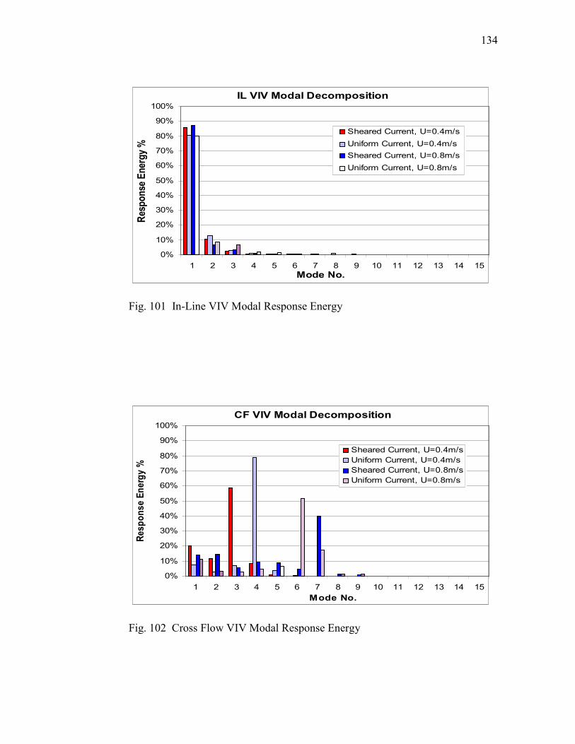
134
IL VIV Modal Decomposition
0%
10%
20%
30%
40%
50%
60%
70%
80%
90%
100%
1 2 3 4 5 6 7 8 9 10 11 12 13 14 15
Mode No.
Response Energy %
Sheared Current, U=0.4m/s
Uniform Current, U=0.4m/s
Sheared Current, U=0.8m/s
Uniform Current, U=0.8m/s
Fig. 101 In-Line VIV Modal Response Energy
CF VIV Modal Decomposition
0%
10%
20%
30%
40%
50%
60%
70%
80%
90%
100%
1 2 3 4 5 6 7 8 9 10 11 12 13 14 15
Mode No.
Response Energy %
Sheared Current, U=0.4m/s
Uniform Current, U=0.4m/s
Sheared Current, U=0.8m/s
Uniform Current, U=0.8m/s
Fig. 102 Cross Flow VIV Modal Response Energy
135
Discussions
In this chapter we presented two case studies with shear current speed of 0.4 m/s
and 0.8 m/s at x/L=1.0. The results are within the ranges of published experiment data. It
indicates that the FANS code is capable of predicting reasonable results for long risers
using fairly coarse grid in the riser axial direction. It is worthwhile to note that FANS
can be readily generalized to handle much more complex current conditions, such as
highly shear current and submerged current. Some findings of the study are:
1. The vortex shedding pattern in the shear current is different from that of the
uniform current. In the uniform current case, the riser motion and vortex
shedding are usually synchronized. In the shear current case, the 2S and C
patterns may correspond to the power-in and power-out zones along the riser.
2. Mode lock-in could occur in the shear current. However, its dominant level
(in terms of the energy percentage) is lower than that of the uniform current.
3. A long marine riser could have large mean lateral deflection when subject to
strong current. It seems that this mean lateral deflection is more than a static
value that could be subtracted during the riser VIV simulations. It is part of
the result from the fluid-structure interaction. Hence it could influence the in-
line and cross flow VIV by altering the flow field.
In conclusion, we used a CFD approach to simulate a long marine riser VIV
response in shear current. The simulation details are presented, analyzed, and validated
against the experiment data (Huang et al. 2007a, 2007b, 2007c, 2007d).

136
CHAPTER VIII
3D SIMULATION OF FLOW PAST A 3000FT RISER
IN UNIFORM CURRENT
This chapter studied the VIV of a hypothetical single casing top tensioned riser
sized for 3,000ft water depth (L/D=3,350). The riser dynamic response under different
currents is simulated in 3D. The riser-fluid interaction effect is included through
instantaneous drag and lift forces. The riser inline and cross flow responses, including
A/D, modal shapes and frequencies, and VIV induced stresses, are studied in detail as
well.
The fluid domain around the riser is meshed with structure data grids, which
consist of a phantom background grid, a wake grid, and a riser body grid. It is estimated
that the highest mode could be excited in a 0.4 m/s current (slightly less than 1 knot) is
the 12th mode. In order to represent this mode, we used 30 data grids in the riser span
direction, which is a minimum. The total element number is kept below 1 million, so the
computation can be performed on a single processor PC. More data grids would
certainly improve the riser simulation accuracy, at the expense of computational speed
and resources. During the simulation the wake grid and body grid move together with
the riser.
The non-dimensional time step used in the simulation is 0.01, which means the
free stream fluid travels a distance of one riser diameter in 100 time steps. This time step
137
is typical for similar riser VIV problems, and is sufficiently small for stable time domain
simulations.
The studied riser is a 10 ¾” single casing top tensioned riser designed for 3,000 ft
water depth. It has a nominal top tension of 400 kips, submerged weight 121 lb/ft, and
mass ratio of 4.0. The riser string consists of steel bare joints without external insulations
and strakes. For simplicity, specialty joints, such as stress joint and tension joint, are
assumed to have the same sectional properties with standard joint. The riser top and
bottom boundary conditions are also simplified as pin connection.
The riser has a fundamental frequency of 38 seconds in seawater. Preliminary
reduced velocity (Blevins, 1990) screening shows the dominant mode is likely to have a
frequency between 8th and 12
th mode. The riser modal shapes have been calculated up to
the 40th mode to cover any high mode vibrations. The selected modal shapes are shown
in Fig. 103. Note that the modal shapes are normalized to unit maximum amplitude,
which is usually located near the riser bottom. For deepwater risers, the effective tension
near the subsea wellheads is minimum, while it increases to its maximum at the top.
Therefore, the peak values of its modal shapes are not constant along the riser. Lower
effective tension results in higher vibrating amplitudes. This causes an interesting
observation: in deepwater applications, the current profiles usually have their maximum
speed near ocean surface, however, the worst riser VIV response is well beyond that
region, and it occurs near the bottom, where the current speed is nearly zero, or no
current at all. It is also worthwhile to note that a typical production riser has slightly
more complicated top and bottom boundary conditions than pinned connection: the
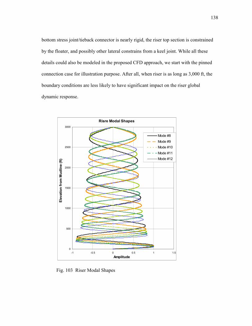
138
bottom stress joint/tieback connector is nearly rigid, the riser top section is constrained
by the floater, and possibly other lateral constrains from a keel joint. While all these
details could also be modeled in the proposed CFD approach, we start with the pinned
connection case for illustration purpose. After all, when riser is as long as 3,000 ft, the
boundary conditions are less likely to have significant impact on the riser global
dynamic response.
Risre Modal Shapes
0
500
1000
1500
2000
2500
3000
-1 -0.5 0 0.5 1 1.5
Amplitude
Elevation from M
udline (ft)
Mode #8
Mode #9
Mode #10
Mode #11
Mode #12
Fig. 103 Riser Modal Shapes

139
Simulation Results
The simulations have been performed for 20,000 time steps, which correspond to
a period of 140 seconds. Fig. 104 shows the evolution of the riser dynamic motion. The
risers are initially straight and have no external force except gravity. At t=0s, the risers
are subject to a uniform or shear current. They deflect to a new equilibrium position and
vibrate back and forth. The in line motions are dominated by transient dynamics. It is not
that straightforward to filter out the in-line transient motions. That is also one reason we
mainly focused the study on cross flow VIV. Another reason is that the expected
dominant mode for in-line VIV is very high (twice of the dominant mode in cross flow
VIV), and it is beyond the riser axial resolution of the data grid we used. Being said that,
the in-line transient motion could also be important to riser VIV in a sense that: (1) it
could influence the riser VIV through disturbing the flow field and changing the initial
conditions for vortex shedding, and (2) in the physical world the current condition
changes continuously. In other words, the transient response would always exist in real
world and might also deserve some attention as well. Some observations from the
snapshots are:
At startup phase, the vortices develop slower in the riser middle section than the
regions near the ends. Since the riser is fixed at its two ends, the relative velocity is close
to the incoming current velocity, and vortices are able to develop and shed when flowing
around fixed cylinders. While in the riser middle section, the riser segment has no lateral
constrain during the initial period and moves downstream with the current, which results

140
in small relative velocity. As a result, the drag coefficients near the riser ends are larger
than that in the middle section.
In shear current, the riser top section is subject to higher current speed than the
lower section. Its initial deflection corresponds to the current profile, i.e. larger riser
deflection at higher speed region. However, as the riser deflects more, its own
characteristics take effect as well. The riser has much higher effective tension at the top
section than in the bottom section. From the riser motion equation we know that the
higher the tension, the stiffer the riser would be in lateral direction. Therefore, even the
riser lower section is subject to lower current speed, it has much more lateral flexibility,
hence has more excursion.
The vortex shedding in the wake of the riser exhibits different patterns at
different time. Initially 2S pattern is clearly seen along the whole riser. When the riser
reaches near its maximum deflection, coalescence of vortex (C pattern) occurs at top and
bottom regions. In shear current case, C pattern occurs only at the top region where the
current speed is the maximum. The vortex shedding maintains 2S pattern below a
transitional section from C pattern to 2S pattern. In the uniform current case, we found
that the C pattern could continue propagating into the middle section of the riser, until it
covers the whole riser. Due to the reduced drag force on the riser, the riser reduces its
lateral deflections dramatically, as indicated by the arrow in the figure. After that the 2S
pattern recovers in the middle section and pushes the riser back toward its equilibrium
position. Figs. 105 and 106 show the vorticity contour snapshots where the vortex
pattern could be clearly identified.

141
Overall, the riser exhibits strong flexibility. The cross flow VIV amplitudes are
also shown in Figs. 105 and 106 for shear and uniform current respectively. As expected,
the shear current causes much less drag force, hence lateral excursion on the riser than
the uniform current. The figures also show that the riser lateral deflection is coupled with
the vortex shedding, and it could introduce complicated dynamic cross flow response,
even in a simple uniform current.
Fig. 104 Riser VIV Comparison, Umax=0.4m/s, Left:Uniform, Right:Shear

142
"C" Pattern
"2S" Pattern
VIV Dominant Region
Fig. 105 Riser VIV Snapshot, Shear Current

143
"C" Pattern
"2S" Pattern
VIV Dominant Region
Fig. 106 Riser VIV Snapshot, Uniform Current
The cross flow modal responses are plotted as shown in Fig. 107. The modal
response below 7th mode and above 12
th mode has been filtered out during the post-
processing for clarity. It shows the dominant mode for the shear current is the 9th mode,
while both the 11th and 12
th modes have significant contribution to the VIV response for
uniform current case. We compared the rms a/D to the results from Shear 7 in Figs. 108
and 109 for uniform current and shear current respectively. It shows the results are
comparable for shear current, while FANS predicts lower response in uniform current.
This is clearly related to the number of dominant modes. It is worthwhile to point out
that other CFD simulations (Willden and Graham, 2004) also showed that the VIV in
uniform current is multi-modal, i.e. several modes with similar frequencies are excited at
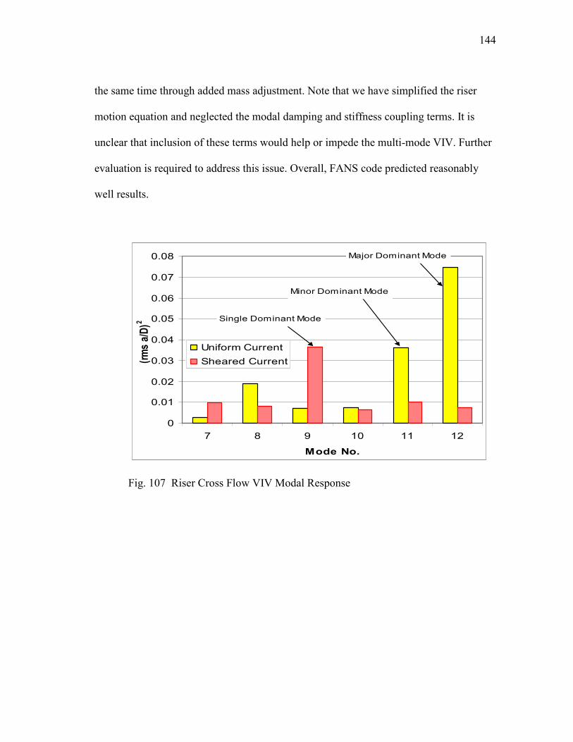
144
the same time through added mass adjustment. Note that we have simplified the riser
motion equation and neglected the modal damping and stiffness coupling terms. It is
unclear that inclusion of these terms would help or impede the multi-mode VIV. Further
evaluation is required to address this issue. Overall, FANS code predicted reasonably
well results.
0
0.01
0.02
0.03
0.04
0.05
0.06
0.07
0.08
7 8 9 10 11 12
Mode No.
(rms a/D)2
Uniform Current
Sheared Current
Single Dominant Mode
Major Dominant Mode
Minor Dominant Mode
Fig. 107 Riser Cross Flow VIV Modal Response

145
CF Motion RMS (Uniform Current, U=0.4m/s)
0
0.1
0.2
0.3
0.4
0.5
0.6
0.7
0 0.2 0.4 0.6 0.8 1
x/L
rms a/D
FANS
Shear 7
Fig. 108 Riser Cross Flow VIV rms a/D - Uniform Current
CF Motion RMS (Sheared Current, U=0.4m/s)
0
0.1
0.2
0.3
0.4
0 0.2 0.4 0.6 0.8 1
x/L
rms a/D
FANS
Shear 7
Fig. 109 Riser Cross Flow VIV rms a/D - Shear Current

146
The stress rms for the uniform and shear currents are presented and compared to
Shear 7 in Figs. 110 and 111 respectively. The comparisons are in general agreement. It
shows in both cases that the worst stress is always near the riser lower end. This is due to
the lower effective tension at the riser bottom portion. This is interesting since in shear
current, the current has high speed at the top, while the VIV-induced fatigue damage at
this location is minimum. In contrast, there is no current near the bottom, while the
fatigue damage at this region is the worst.
CF Stress RMS (Uniform Current, U=0.4m/s)
0
1
2
3
4
5
6
7
0 0.2 0.4 0.6 0.8 1
x/L
Stress rms (ksi)
FANS
Shear 7
Fig. 110 Riser Cross Flow VIV Induced Stress – Uniform Current

147
CF Stress RMS (Sheared Current, U=0.4m/s)
0
0.5
1
1.5
2
2.5
3
0 0.2 0.4 0.6 0.8 1
x/L
Stress rm
s (ksi)
FANS
Shear 7
Fig. 111 Riser Cross Flow VIV Induced Stress – Shear Current
Discussions
In this chapter we have studied a 3,000ft riser VIV under both uniform and shear
current conditions. The fluid-riser interactions are simulated in time domain. The riser
3D motion and vortex shedding pattern are examined in detail. We also calculated the
cross flow VIV amplitudes and stress rms along the riser, and compared with the results
obtained from Shear 7 (Huang el al., 2007a, 2007d). It is found that the riser could
experience multi-mode VIV in uniform current. It is also found that the CFD approach
provides reasonable results. Hence it is feasible for deepwater riser VIV assessment.
Further work is recommended in areas including (1) riser initial condition and its
transient effect on VIV, and (2) riser modal coupling effect on VIV.
In conclusion, an effective CFD approach has been presented and applied to
practical riser VIV assessment.

148
CHAPTER IX
3D SIMULATION OF FLOW PAST A CANETARY RISER
IN UNIFORM CURRENT
As more and more oil and gas field developments are in deepwater regions and
harsh environments, how to install the subsea equipment and flowlines safely and
efficiently becomes a challenging subject that might require the support from the latest
technologies. During a recent offshore subsea installation project in Offshore Brazil,
some interesting phenomena were observed: (1) the flexible riser deflection in the water
column was much higher than expected when subject to strong currents; (2) the curve on
the sea floor tended to lose stability in a much lower current condition than predicted.
Consequently, it caused difficulties and temporary schedule delay for the flexible riser
installation. This paper is intended to realize what occurred to the flexible riser when it
was subjected to strong currents, and provide theoretical evidence to support future
engineering practice improvement and offshore installation guidelines (Huang et al.,
2010).
Offshore Brazil is well known for the strong bottom current. The field measured
current speed was up to 1.2 knot near the seabed. A recent project involved installation
of more than 100 km of flexible flowlines and risers in a field located in the northern
Campos Basin approximately 220 km northeast of Macae. It consisted of individually
completed subsea production wells with gas lift and water injection wells tied back to a
floating, production, storage, offloading (FPSO) vessel with flexible flowlines. The field

149
layout was fairly congested due to the sea bed bathymetric constrains, and included a
number of sharp turns and low-radius curves. Engineering analytical work was done
extensively to ensure smooth offshore installation operations. It worked well except for
the flexible flowline curve laying in strong currents, which experienced some delay
because the flexible flowline failed to maintain its position on the seabed and slipped out
of its lay corridor. A snapshot of the plane view during the curve laying is illustrated in
Fig. 112. The dotted line is the designed flowline position, or the target position to land
the flowline onto during the installation. The solid line is the actual flowline position.
The flowline is paid out from the installation vessel continuously, and it is suspended in
the water column until it reaches the sea floor at the touchdown point (TDP). When
strong current exists (most of the time it is from south), the flowline is pushed toward
north due to the current drag force. Therefore, the catenary shape is bended toward
north. The installation vessel monitors the flowline TDP and adjusts its position
accordingly to ensure the flowline is laid within the allowable corridor. The illustrated
flexible flowline was part of a production loop that begins and ends at the FPSO. Its field
layout includes a 130m-radius curve to turn the flow direction back to the FPSO, as the
dotted line indicates. The curve is stable if the soil friction is sufficient to hold the pipe
in place against the bottom tension. Otherwise the curve won’t be able to maintain
(slippage occurs, as illustrated by the dashed line in Fig. 112). Pipe-soil friction
coefficient was determined by the pipe and soil properties, and not related to the current.
Therefore, the flexible flowline bottom tension becomes the controlling parameter for
curve stability during installation, and it is directly related to the current strength. The
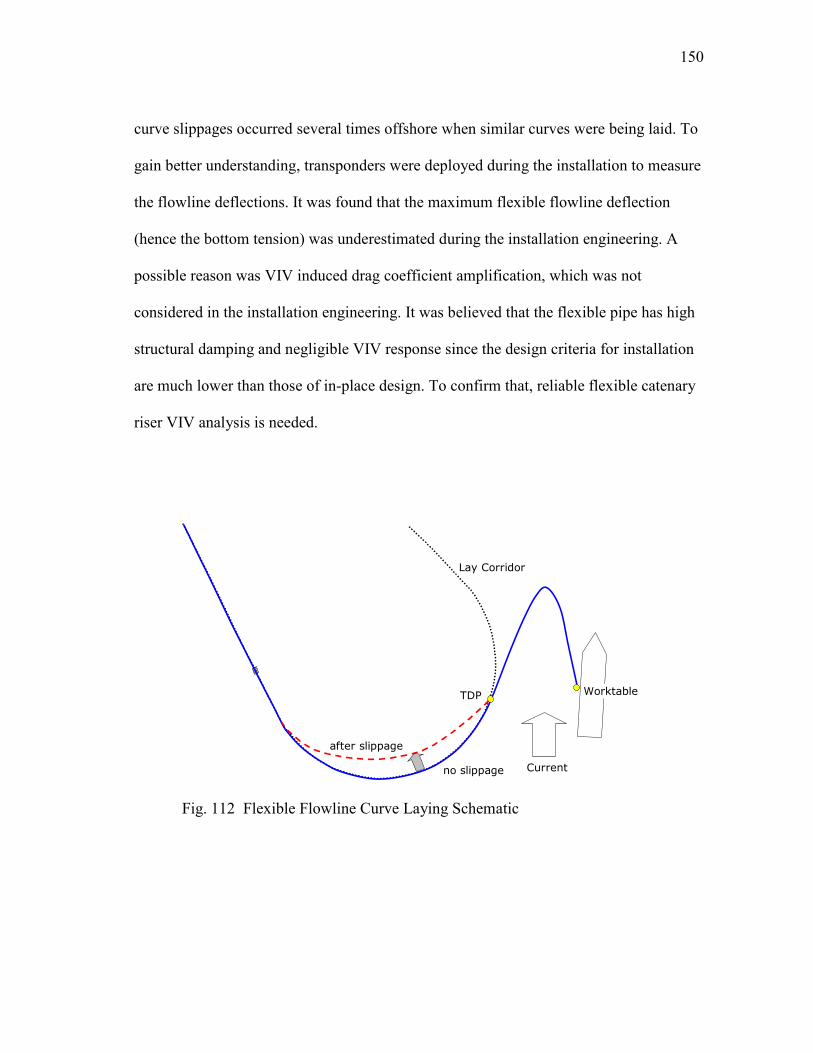
150
curve slippages occurred several times offshore when similar curves were being laid. To
gain better understanding, transponders were deployed during the installation to measure
the flowline deflections. It was found that the maximum flexible flowline deflection
(hence the bottom tension) was underestimated during the installation engineering. A
possible reason was VIV induced drag coefficient amplification, which was not
considered in the installation engineering. It was believed that the flexible pipe has high
structural damping and negligible VIV response since the design criteria for installation
are much lower than those of in-place design. To confirm that, reliable flexible catenary
riser VIV analysis is needed.
TDP Worktable
Lay Corridor
after slippage
no slippage Current
Fig. 112 Flexible Flowline Curve Laying Schematic

151
As of today there are very few publications on the flexible catenary flowline/riser
VIV. Some of the reasons are: (1) the flexible flowlines are still relatively new for
industrial deepwater application; (2) the flexible flowlines have good fatigue resistance
performance and high structural damping, therefore, VIV induced fatigue was not as
critical as the steel pipe risers; (3) the flexible flowlines consist of multiple layers that
serve as different functions and have different material properties. The combined cross
sectional properties are non-linear, project specific, and difficult to obtain and model; (4)
The configuration and general layout of the flexible riser system are versatile and
complex, and typically involve one or more catenary shapes, and also possibly other
auxiliary components, such as buoyancy modules, buoys, clamps, bending
restrictors/stiffeners etc. To the authors’ knowledge, this study is the first among its kind
to investigate a flexible catenary riser VIV using CFD approach.
In fact the flexible flowlines have been increasingly used for deepwater and
ultra-deepwater field applications, partially because of their fatigue resistance
performance and low submerged weight.
It is estimated that the linearized bending stiffness of the subject flexible flowline
is about 100 kN-m2. During its installation, a layback distance of 100 m was used, which
corresponded to 1 deg nominal departure angle at the worktable. The suspended length
of the flexible riser is 1,100m (L/D=3,300). The current speed could ramp up quickly, in
terms of several hours, from near zero to a peak value ranged from 0.7 knot to 1.2 knot.
ROV was sent to measure the current profile from time to time. It was found that the
current profiles were fairly uniform starting from the sea bed to about 200 m below the
152
mean surface line. For the sake of simplicity, we used uniform current of 0.7 knot
throughout the water column for the VIV simulation.
In the present simulations, the flow field around the riser was discretized by 1.5
million finite elements, and solved numerically in time domain. The riser lateral
displacement was decomposed into three components: (1) catenary shape due to the riser
weight, (2) in plane motion due to the current drag force, and (3) out-of-plane motion
due to the lift force. The total riser deflection was the superposition of these three
components. The flexible flowline maximum deflections and equivalent drag
coefficients were studied and compared to the field measurements.
The data grid is shown in Fig. 113. It consists of 3 overlapping parts that serve
different purposes: (1) body grid – the data grid adjacent to the riser surface that
provides fine resolution to calculate the fluid-riser surface interaction and vortex
generation, it has dimensions of 50 x 182 x 35, (2) wake grid – it interfaces with body
grid and background grid and provides good resolution for vortex propagation, it has
dimensions of 50 x 121 x 101, (3) background grid –it defines the outer boundary of the
computational fluid domain, provides the far field flow boundary conditions, interfaces
with and provide a physical extension to the wake grid using relatively coarse mesh. It
has dimensions of 50 x 121 x 91.
The flexible riser was also discretised into 250 segments. Its lateral displacement
consists of three components as follows:
1. The static catenary shape. For a flexible flowline with uniform cross section,
its catenary shape is given by: ha
xLaz −
−
+= 1cosh , where L is the

153
layback distance, h is the vertical distance between the flexible flowline
hang-off position to its TDP on the seabed, a is a constant determined by the
departure angle: ( )βcotsinh 1−=
La , and β is the nominal departure angle.
The origin of the coordinate system was chosen at the worktable (the flexible
pipe hang-off location). The static catenary shape is always in the vertical
plane determined by the worktable location and the flexible flowline TDP.
2. Riser response due to the drag force. The response can be decomposed into in
plane and out of plane components. Note that the drag force is time
dependant, and was calculated by integrating the pressure force and viscous
force along the riser surface in the current flowing direction.
3. Riser response due to the lift force. The response can be decomposed into in
plane and out of plane components. It was calculated by integrating the
pressure force and viscous force along the riser surface in perpendicular to
the current flowing direction.
The riser instantaneous displacement is the summation of the above three
displacement vectors at each time step. The main advantages of this method are: (1) the
catenary shape is calculated statically, and simple catenary equation could be used. This
would avoid a complex dynamic catenary solver, (2) a simple tensioned beam motion
equation was applied to calculate the riser dynamic vibrations. This equation has a fairly
stable differential scheme, and provides reliable solution to the riser motions. The
disadvantage is that it is difficult to include the pipe-soil interaction into this simplified

154
model. Since in this study the primary focus is on the overall flexible flowline VIV
behavior and its impact on the effective drag coefficient, this model provides sufficient
performance.
Fig. 113 Data Grid along the Flexible Riser
Modal analysis was performed to provide the modal frequencies and modal
shapes. The modal shapes were separated into in plane modes and out of plane modes
based on vibrating planes. The fundamental frequencies are 98 seconds for in plane and
122 seconds for out of plane respectively. Fig. 114 compares the normalized modal
shapes of the in plane and out of plane fundamental modes. It shows that the in plane

155
mode has different behavior from the out of plane mode. The in plane mode has two
peaks. Except the major peak (normalized to 1.0), it also has a minor peak about -0.15
near the TDP region. When the flexible flowline has in plane deflection, its TDP will
move in the opposite direction. This would reduce the effective length of the modal
shape, and increase the modal frequency. It is one reason that the in plane fundamental
modal frequency is slightly higher than that of the out of plane. Other reasons are the
added mass difference and static curvatures. When the flexible flowline vibrates in the
catenary plane, its velocity direction is not perpendicular to the flexible flowline.
Therefore, the effective added mass coefficients are less than that of the out of plane
case. Also the static curvature (from the catenary shape) could impact the flexible
flowline behavior as well. The modal frequencies of the first 10 modes are listed in
Table 4. It shows the discrepancy between the modal frequencies for the in plane and the
out of plane modes reduces when the modal number increases. This is expected since the
vibration becomes more and more localized for high modes. And in high modes the local
curvatures increase dramatically such that the catenary shape induced curvature (static
curvature) has negligible effect on the local behavior.

156
Table 4 Flexible Catenary Riser Modal Frequency
Out of Plane In Plane Mode
No T (sec) f (Hz) T (sec) f (Hz)
1 122.0 0.008 97.8 0.010
2 59.2 0.017 50.2 0.020
3 39.2 0.025 34.1 0.029
4 29.3 0.034 25.9 0.039
5 23.4 0.043 21.0 0.048
6 19.5 0.051 17.6 0.057
7 16.7 0.060 15.2 0.066
8 14.6 0.068 13.4 0.075
9 13.0 0.077 12.0 0.084
10 11.7 0.086 10.8 0.093
Fundamental Modal Shape - Inplane vs Out of Plane
-0.2
0
0.2
0.4
0.6
0.8
1
1.2
0 200 400 600 800 1000 1200
Curve Linear Length (m, from worktable)
Amplitude (m)
Inplane
Out of Plane
Fig. 114 Flexible Catenary Riser Fundamental Modal Shapes

157
Simulation Results
In the simulation, 0 degree current heading was used (or the current is from the
far direction). This is the worst condition for the flexible flowline curve stability since it
gives the maximum bottom tension at the TDP. The current speed was 0.7 knot. This
speed was observed frequently during offshore installation and was selected for this
study. It corresponds to a Reynolds number of 1.05 x 10⁵. The time step for the numerical
simulation was chosen as 0.009 s, which is sufficiently small for the dominant modes. The
duration of the simulation is 20,000 time steps, or 180 seconds. Fig. 115 illustrates the
flexible riser deflection and vortex development and shedding process. The flexible riser
started with a static catenary shape. When it was subject to strong current, it deflected in
current direction due to the drag forces. At the same time, it also started cross flow
vibrations due to the lift forces.
The results showed that the maximum riser deflection was near the bottom
region, where the effective tension was low. Typically the flexible flowline bottom
tension was around 1~2 Te, while the top tension could be more than 20 Te. The bottom
tension is adjustable in a limited range by positioning the installation vessel and varying
the layback distance. Nevertheless, the bottom tension of a catenary riser is always low
regardless of the flexible riser properties. It is expected that the flexible riser behavior
near the bottom is different from its upper portion because of this low tension
characteristics, and it is common among all catenary risers.

158
Fig. 115 Flexible Catenary Riser VIV Evolution Illustration (Top View)

159
Flexible Cross Flow VIV rms a/D
0
0.2
0.4
0.6
0.8
1
1.2
1.4
1.6
1.8
0 0.1 0.2 0.3 0.4 0.5 0.6 0.7 0.8 0.9 1
x/L
rms a/D
Fig. 116 Cross Flow VIV rms a/D, U=0.7knot
The flexible flowline VIV includes both in plane and cross flow vibrations.
Usually the VIV amplitudes are in the order of 1D, which is negligible comparing to the
flexible flowline in plane deflection. Therefore, the in plane VIV is of less interest. The
cross flow VIV rms a/D was plotted in Fig. 116. x/L=0 corresponds to the bottom of the
flexible flowline (TDP), while x/L=1.0 corresponds to the top of the flexible flowline
(worktable). It shows the flexible flowline experienced cross flow VIV, and its rms a/D
distribution consists of two portions:
• The upper portion with rms a/D ranging from 0.2 to 0.6. This range is
consistent with a typical top tensioned riser. The rms a/D indicates a
downward trend when x/L increases. This is expected since the riser tension

160
increases as the elevation gets higher. And the response rms a/D correlates to
the tension distribution very well.
• The bottom portion with rms a/D as high as 1.5. This response is very high.
Seems it is related to the near-zero bottom tension. This region includes the
lowest 20% of the total riser length.
Overall, the results indicate that the catenary riser VIV will have different VIV
response pattern than the top tensioned risers. Its low tension / near-zero tension zone
could show complicated behavior that requires particular attention during numerical
simulations. It also indicates that the dominant modes should be less than the 10th mode,
based on the rms a/D distribution shapes.
The flexible flowline maximum in plane displacement is a critical parameter of
this VIV study. During offshore installation transponders were attached onto the flexible
flowlines to identify the actual catenary shape when strong current exists. It was found
that the flexible flowline could be pushed 80 m to 90 m away from the vertical line at the
worktable when the measured current was around 0.7 knot. Fig. 117 shows the flexible
flowline maximum deflection from the VIV simulation. The maximum deflection of 70
m occurs near the bottom. Considering the uncertainty of the field measured current
profile and the varying nature of the current speed and direction, the flexible flowline
maximum deflection from the VIV simulation is in a reasonable range. The flexible
flowline deflection is quite large, and excessive riser displacement causes problems such
as: (1) lose curve stability when the current is from the far or cross direction; (2) lose
control of flexible flowline laying at the TDP, form pig tail loops on the sea floor and
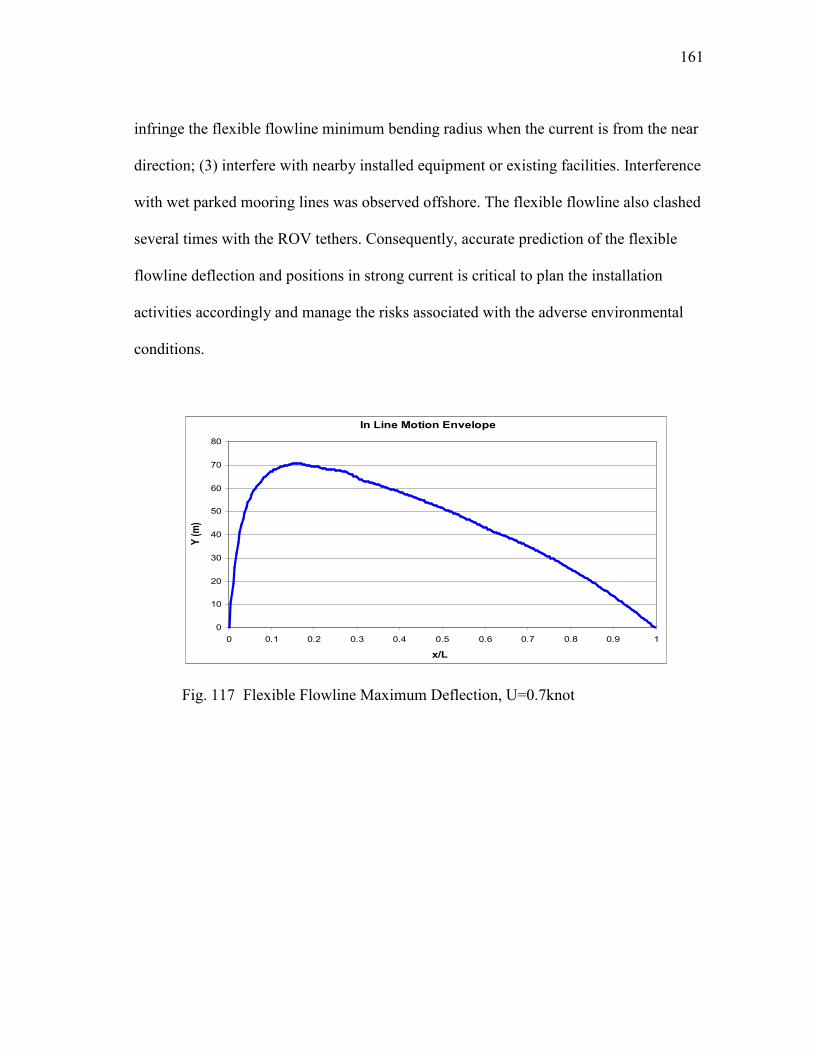
161
infringe the flexible flowline minimum bending radius when the current is from the near
direction; (3) interfere with nearby installed equipment or existing facilities. Interference
with wet parked mooring lines was observed offshore. The flexible flowline also clashed
several times with the ROV tethers. Consequently, accurate prediction of the flexible
flowline deflection and positions in strong current is critical to plan the installation
activities accordingly and manage the risks associated with the adverse environmental
conditions.
In Line Motion Envelope
0
10
20
30
40
50
60
70
80
0 0.1 0.2 0.3 0.4 0.5 0.6 0.7 0.8 0.9 1
x/L
Y (m)
Fig. 117 Flexible Flowline Maximum Deflection, U=0.7knot

162
The flexible flowline effective drag coefficient is also of interest since it is a
normal practice to use an effective drag coefficient instead of time consuming CFD
approach for offshore installation engineering. Current design codes (such as API RP
2RD) provide drag coefficient selection criteria, which depend on Reynolds number. In
the studied case the Cd is between 1.0 to 1.2 for Re=105 for a fixed cylinder. When the
cylinder undergoes VIV in current, the effective drag coefficient could be higher because
the riser lateral movement increases the equivalent drag area. The drag coefficient was
calculated during the VIV simulations at each time step and each location along the riser.
The instantaneous drag coefficient depends on the riser movement and flow field
condition, and may vary dramatically in a wide range. Its impact on the riser deflection
is mainly determined by the time-averaged value. Fig. 118 shows the average Cd
distribution along the riser. It shows that the drag coefficient of the riser upper portion is
between 1.0 to 1.5. At the riser bottom, the drag coefficient varies in a larger range, from
0.5 to 2.5. Some observations are as follows:
1. By comparing Fig. 118 to Fig. 116, it shows the drag coefficient at the riser
bottom has strong correlation to the cross flow VIV amplitude at that region.
The drag coefficient could be either amplified or suppressed significantly.
2. The VIV induced Cd amplification is obvious at the top half of the riser,
where its tension is high.
3. The average Cd along the riser is approximately 1.3, which is 10~20% higher
than the Cd for the fixed riser condition.

163
Overall, the results indicated that for catenary risers, high VIV amplitude does
not necessarily result in high effective Cd. A possible reason could be the dominant VIV
response frequency. The catenary risers have very long fundamental modal frequencies.
Based on a Strouhal number of 0.2, it is estimated that the vortex shedding frequency is
0.21 Hz (4.7 s), which corresponds to the 23rd modal frequency. However, it is unlikely
that the 23rd mode could be excited since the flexible flowline has high structural
damping that tends to dampen out any high frequency vibrations. This can be confirmed
from Fig. 116 since it does not show any indications of high frequency modal response.
Average Cd Distribution
0
0.5
1
1.5
2
2.5
0 0.1 0.2 0.3 0.4 0.5 0.6 0.7 0.8 0.9 1
x/L
Cd
Fig. 118 Drag Coefficient Distribution, U=0.7knot

164
Discussions
This chapter studied a flexible riser VIV using a CFD approach. The flexible
riser parameters and environmental conditions were obtained from a recent installation
project in offshore Brazil. During the offshore installation, it was found that the flexible
riser could have higher lateral deflection than expected when subject to strong current.
The selected case was simulated in time domain using proven CFD technology in
conjunction with a simplified catenary riser motion solver. The simulation details were
presented, and the maximum riser deflection was also compared to the field
measurement. It is found that:
1. The flexible riser VIV response is complicated by its low tension at its
bottom section (near seabed region). In this region the flexible riser could
have large VIV response and sensitive drag coefficients.
2. The flexible riser VIV response reduces along the riser and reaches its
minimum at the top. This distribution correlates well to the riser effective
tension distribution. It confirms that high tension would result in low VIV
response.
3. The average effective drag coefficient is up to 20% higher than the fixed riser
condition. A maximum deflection of 70 m was observed in the riser VIV
simulation with uniform current speed 0.7 knot, which is consistent with
offshore observations.

165
Note that the present approach could be further improved by refining the
catenary riser motion solver. Some recommendations are:
1. Inclusion of the riser-soil interaction. When the riser moves, the riser TDP
also moves, both axially and transversely. And the riser section on the seabed
will experience both the vertical loads and lateral friction force. These
nonlinear behaviors need to be modeled in order to accurately predict the
riser bottom VIV response.
2. Inclusion of the flexible flowline bending hysteretic curves. The flexible
flowline has strong nonlinear properties, especially the bending stiffness.
In summary, the simplified catenary riser motion solver worked well, and the
simulation results are reasonable. The results showed that the flexible riser VIV could
increase the effective drag coefficient by 10~20%, which partially explains the
phenomenon of high flexible riser deflection observed offshore.

166
CHAPTER X
3D SIMULATION OF FLOW PAST A PARTIALLY SUBMERGED
JUMPER IN UNIFORM CURRENT
This chapter studied the VIV of a flexible jumper. Flexible jumpers are widely
used in oil and gas industry to transport liquid or gas content between two facility units,
usually located close to each other and have relative movement. In many of its
applications, the jumper is positioned near the water surface, sometimes surface piecing,
hence subject to severe environmental loads, including strong surface currents. This
paper is to study a flexible jumper VIV in uniform current by using a CFD simulation
approach (Huang et al., 2011).
Fig. 119 shows a typical jumper arrangement. In this hypothetical case the
jumper’s first end is attached to a submerged facility at 50 m below the mean surface
level, and its second end is attached to a hang-off porch at 30 m above the mean surface
level. The nominal horizontal span is 200 m. The jumper has a diameter of 0.33 m, and
total length is 265 m (L/D=800). Its air weight is 100 kg/m, and submerged weight 20
kg/m (mass ratio=1.0). The mass ratio is 2/ Dm ρ (Vandiver, 1993). A uniform current of
0.5 m/s (1knot) is applied in the direction perpendicular to the jumper catenary plane.

167
200m
50m
30m
MeanSurface Line
jumper
Fig. 119 Jumper General Arrangement
This study is the first to study the surface piecing cylinder VIV using 3D CFD
simulation approach. The publications on VIV 3D simulation of catenary risers are rare,
except for the one we published on a flexible riser VIV (Huang, Chen & Chen 2010).
This study is a continuous effort on the VIV simulations on catenary type of risers. The
main challenges of the jumper VIV simulation are:
1. The jumper tension level is fairly low. The jumper could have large lateral
deflection when subject to strong current flow. This lateral movement causes
high deformation on the data grids, and imposes difficulty on fluid-structure
solver. And very fine time steps have been used in the simulation to ensure
the simulation accuracy.
2. The apparent mass distribution along the jumper is not uniform, and
disconnection exists at the mean surface level. The jumper configuration

168
cannot be represented by the simple catenary equation. A trial and error
approach is proposed in this paper to calculate the catenary shape. The non-
uniform apparent mass distribution also requires fine mesh on the riser.
3. The effective tension distribution is non-linear and its amplitudes vary in a
large range. The modal shapes also show strong non-linear behavior, and are
not orthogonal to each other. In order to extract the modal components, a
least squares method is adopted.
4. The jumper cross flow VIV response could be influenced by the lateral
motions, and contains transient dynamic response. A filtering methodology is
presented in this paper to better interpret the VIV response results and
characteristics.
In this study we first developed a static catenary solver to determine the jumper
configuration. The upper section (about 10% of overall length) of the jumper is in the
air, and the lower section (about 90% of the overall length) is submerged in the water.
The static catenary solver is capable of handling cable catenary shapes with arbitrary
mass distributions. Then the modal frequencies and modal shapes were derived and
examined. The jumper cross flow transient response was also simulated and its modal
component distribution was studied. After that a uniform current of 1 knot was imposed
as far field incoming current, and the jumper dynamic responses were simulated in time
domain. The vortex shedding details were plotted and examined. The cross flow VIV
rms a/D was also calculated and compared to the results predicted by Shear 7. Other
important parameters, including dominant modes, modal components, and motion
169
trajectories, were derived and studied as well. It is found that the jumper cross flow VIV
may contain more than one modes with similar strength. And the VIV amplitudes
correlate well to the effective tension distribution. It is also noticed that the jumper
motion trajectories show complex behavior, and may not follow figure “8” pattern. In
conclusion, the jumper VIV was simulated in time domain, and reasonable results were
obtained. The validity of the proposed CFD approach was also confirmed through the
results comparisons.
The data grid is shown in Fig. 120. It consists of 3 overlapping parts that serve
different purposes: (1) body grid – the data grid adjacent to the jumper surface that
provides fine resolution to calculate the fluid-jumper surface interaction and vortex
generation, it has dimensions of 50 x 182 x 35, (2) wake grid – it interfaces with body
grid and background grid and provides good resolution for vortex propagation, it has
dimensions of 50 x 121 x 101, (3) background grid –it defines the outer boundary of the
computational fluid domain, provides the far field flow boundary conditions, interfaces
with and provide a physical extension to the wake grid using relatively coarse mesh. It
has dimensions of 50 x 121 x 91.
The non-dimensional time step is selected to be 0.01 (fluid particle travels 1
diameter distance in 100 time steps), which is sufficiently small to avoid possible
numerical instabilities and ensure calculation accuracy.

170
Fig. 120 Data Grid along the Flexible Jumper
Simulation Results
In the simulation, a uniform current perpendicular to the jumper catenary plane
was applied. The current has a velocity of 0.5 m/s. It corresponds to a Reynolds number
of 1.5 x 10⁵. The dimensional time step for the numerical simulation was chosen as 0.0066
s, which is sufficiently small for the dominant modes. The duration of the simulation is
20,000 time steps, or 130 seconds. The flexible jumper started with a static catenary shape.
When it was exposed to the uniform current, it deflected in the current direction due to the
drag forces. At the same time, it also started cross flow vibrations due to the lift forces.
Fig. 121 shows one snap shot of the jumper undergoing VIV at time step=20,000. Note
that the top portion of the jumper is above the mean surface line, and the vortex shedding
occurs only on the submerged portion of the jumper.
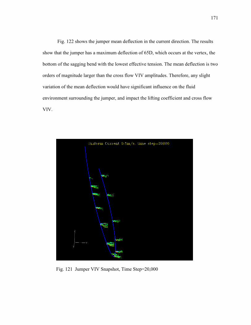
171
Fig. 122 shows the jumper mean deflection in the current direction. The results
show that the jumper has a maximum deflection of 65D, which occurs at the vertex, the
bottom of the sagging bend with the lowest effective tension. The mean deflection is two
orders of magnitude larger than the cross flow VIV amplitudes. Therefore, any slight
variation of the mean deflection would have significant influence on the fluid
environment surrounding the jumper, and impact the lifting coefficient and cross flow
VIV.
Fig. 121 Jumper VIV Snapshot, Time Step=20,000

172
Jumper In-line Deflection
0
10
20
30
40
50
60
70
80
0 0.2 0.4 0.6 0.8 1
s/L
Mean
Deflection / D
In-line Deflection
Fig. 122 Jumper Mean Deflection due to Current Drag Force
In general, the vortex shedding shows clear “2S” pattern (Williamson and
Roshko, 1988) along the jumper. Fig. 123 and 124 show the snap shots (time
step=18,600) of the vortex shedding and vorticity contours at two locations: s/L=0.25
and s/L=0.5 respectively. At each location, the vortex shedding details on three adjacent
stations (spaced at 15D apart along the jumper) were plotted. It shows that the vortex
shedding frequency and vorticity contour are very similar within this +/-15D span. It can
also be observed that the vortex shedding phase angle (relative to the jumper) shifts
gradually along the jumper. If the jumper were rigid and fixed (no movement), the
vortex shedding along the jumper would be very similar. Therefore, it seems the jumper
motion is the main reason of this vortex shedding phase angle difference. On the other
hand, the jumper movement could also be inferred from the vortex shedding behavior as
well:
173
• The forming vortex always follows after the jumper cross flow motion, i.e.
the forming vortex is below the jumper when the jumper moves up, and the
forming vortex is above the jumper when the jumper moves down.
• The vorticity contour indicates the vortex separating distances. A decreasing
vortex spacing indicates the jumper moves forward in the current direction,
and a increasing vortex spacing indicates that the jumper is moving back
against the current.
The vortex shedding pattern also provides indications of the power in and power
out zones. In the present case, the jumper is subject to uniform current, and the power in
and power out zones correspond to the whole span of the submerged portion.
The flexible jumper VIV includes both in plane and cross flow vibrations.
Usually the VIV amplitudes are in the order of 1D, which is negligible comparing to the
jumper in-line deflection (two orders higher). As a result, the in-line VIV is obscured by
the deflection variation. It is also of less interest than the cross flow VIV from practical
application point of view. The cross flow VIV rms a/D along the jumper was plotted in
Fig. 125. As a comparison, the results predicted by the Shear 7 were also included. The
Shear 7 calculations were based on recommended default parameter values. Both Shear
7 and FANS predicted the cross flow is dominated by the 5th mode. Discrepancies exist
on the peak value envelopes. Overall FANS predicted lower rms a/D, especially when
s/L>0.3. Possible reason is that Shear 7 assumed a single mode (5th mode) lock-in, while
FANS is based on fluid-structure interactions, and is not selective among any
participating modes. Actually the time domain simulation by FANS has shown the 6th

174
mode was also excited with slightly less energy than the 5th mode. In other words, Shear
7 assigned 100% of the VIV response energy to the 5th mode, while FANS predicted that
the VIV response energy was largely shared between the 5th and the 6
th modes. This also
explains the slight difference of the peak and trough positions along the jumper.
Nevertheless, the results show reasonable agreement between FANS and Shear 7, with
consideration of the different VIV prediction methodologies.
Fig. 123 Jumper VIV Vortex Shedding Pattern, s/L=0.25

175
Fig. 124 Jumper VIV Vortex Shedding Pattern, s/L=0.5

176
Cross Flow VIV Response rms a/D
0
0.1
0.2
0.3
0.4
0.5
0.6
0.7
0.8
0.9
0 0.1 0.2 0.3 0.4 0.5 0.6 0.7 0.8 0.9 1
s/L
rms a/D
FANS
Shear 7
v
Fig. 125 Cross Flow VIV rms a/D
The jumper cross flow motion time histories were decomposed into modal
response, and the rms a/D for each modal component is presented in Fig. 126. The top
figure is the modal components of the total motion, and the bottom figure is the filtered
modal components, which represent the cross flow VIV response better. The modal
components of the transient response were estimated to be i
i erms 1412.04116.0 −= , i=1 to 25.
The filtered modal components show that the jumper cross flow VIV is dominated by
the 5th mode, which contributes more than 60% of the cross flow VIV energy (measured
by 2
irms ). The 6th mode was also excited, and it contributes about 40% of the VIV
energy. Other modes may also exist, but with insignificant contributions. This multi-
modal response observation is consistent with Willden and Graham (2004).

177
y = 0.4116e-0.1412x
0
0.1
0.2
0.3
0.4
0.5
0.6
1 2 3 4 5 6 7 8 9 10 11 12 13 14 15 16 17 18 19 20 21 22 23 24 25
rms a/D
Total rms a/D
0
0.1
0.2
0.3
0.4
0.5
0.6
1 2 3 4 5 6 7 8 9 10 11 12 13 14 15 16 17 18 19 20 21 22 23 24 25
Modal Number
rms a/D
Filtered rms a/D
Fig. 126 Jumper Motion Modal Decomposition
The jumper motion trajectories were plotted at eight stations: s/L=0.1, 0.2, 0.3,
0.4, 0.5, 0.6, 0.7, 0.8, as shown in Fig. 127. The horizontal axis is the current flow
direction, and vertical axis is in the cross flow direction. The trajectories were plotted in
the same scale to facilitate the comparison. The trajectories confirmed that the jumper
VIV behavior in 3D is much more complex than in 2D (rigid cylinder motions), where
the trajectories usually follow figure “8” or deformed figure “8” pattern. The jumper
motion does not exhibit regularity. Instead, it shows certain degree of random behavior.
The main reason is the lateral offset fluctuations. The mean lateral offset could vary in a
range of 1D near the two ends, and up to 8D at the central portion of the jumper.

178
-2
-1.5
-1
-0.5
0
0.5
1
1.5
2
0 10 20 30 40 50 60 70
In-line Displacement / D
Cross Flow Displacement / D
s/L=0.1
-2
-1.5
-1
-0.5
0
0.5
1
1.5
2
0 10 20 30 40 50 60 70
In-line Displacement / D
Cross Flow Displacement / D
s/L=0.2
-2
-1.5
-1
-0.5
0
0.5
1
1.5
2
0 10 20 30 40 50 60 70
In-line Displacement / D
Cross Flow Displacement / D
s/L=0.3
-2
-1.5
-1
-0.5
0
0.5
1
1.5
2
0 10 20 30 40 50 60 70
In-line Displacement / D
Cross Flow Displacement / D
s/L=0.4
-2
-1.5
-1
-0.5
0
0.5
1
1.5
2
0 10 20 30 40 50 60 70
In-line Displacement / D
Cross Flow Displacement / D
s/L=0.5
-2
-1.5
-1
-0.5
0
0.5
1
1.5
2
0 10 20 30 40 50 60 70
In-line Displacement / D
Cross Flow Displacement / D
s/L=0.6
-2
-1.5
-1
-0.5
0
0.5
1
1.5
2
0 10 20 30 40 50 60 70
In-line Displacement / D
Cross Flow Displacement / D
s/L=0.7
-2
-1.5
-1
-0.5
0
0.5
1
1.5
2
0 10 20 30 40 50 60 70
In-line Displacement / D
Cross Flow Displacement / D
s/L=0.8
Fig. 127 Jumper Motion Trajectory
179
Discussions
This chapter studied a partially submerged flexible jumper VIV using a CFD
approach. The flexible jumper size and arrangement are based on a hypothetical offshore
field application case. The simulation results, including vortex shedding details, rms a/D,
modal analysis, modal decomposition, and motion trajectory were presented. The cross
flow rms a/D was also compared to those calculated by using Shear 7, and reasonable
agreements were observed. The conclusions are:
1. The jumper modal shapes are not orthogonal. The least squares method
works well for modal extraction, and is able to extract any number of modal
components. It is recommended to include all the modes below the cut-off
mode, which is determined through the reduced velocity range.
2. The flexible jumper VIV response is complicated by its large lateral
deflection, which is two orders of magnitude higher than the cross flow VIV
amplitudes. Slight change of the drag force is equivalent to relocate the
jumper to a new equilibrium position, and consequently influence the cross
flow VIV response. On the other hand, the jumper in-line mean offsets and
motions need to be carefully considered during jumper VIV time domain
simulation because of their influence on the simulation results.
3. The modal response of the transient effect could be approximated by an
exponential function, which provides an option to filter the transient response
from cross flow VIV.

180
4. The dominant mode may not necessarily be locked-in. The simulation results
showed the dominant mode may allow the co-existence of other participating
modes with similar strength.
5. The jumper motion trajectories are not likely to follow simple figure “8”
patterns, as typically seen in 2D or rigid cylinder VIV. This suggests that the
long catenary cylinder VIV may intrinsically include certain degree of
random behavior, and require statistically approach to gain better
understanding.
In summary, a simplified catenary riser motion solver has been applied to the
VIV simulation of a partially submerged jumper, and it worked well. The time domain
simulations showed reasonable results, and disclosed valuable details on the jumper
VIV. The paper also presented the methods for modal components extraction and
transient response filtering, which are essential for jumper VIV results interpretation. It
also confirmed that the present approach is valid for catenary jumper VIV simulation,
and is applicable for complex VIV problems involving partially submerged risers,
flowlines, jumpers, and cables.

181
CHAPTER XI
SUMMARY AND CONCLUSIONS
In this dissertation we have successfully simulated the VIV of some long risers in
uniform and shear currents. We developed a riser modal motion solver and a direct
integration solver to calculate riser dynamic motions when subject to external forces.
The direct integration solver provides good flexibility on inclusion of riser bending
stiffness and structural damping coefficients. We also developed a static catenary riser
solver based on trial and error iteration technique, which allowed the motion solvers to
handle catenary risers and jumpers with arbitrary mass distributions. We then integrated
the riser motion solvers to the existing FANS code, and applied to a series of riser VIV
problems. First, we simulated the flow field around a fixed and a vibrating riser, and
compared the flow field to Huse’s formula (experimental data). The simulation results
show good agreement, which confirms the effectiveness of both the FANS codes and
data grids. At the same time, we disclosed the “high speed” zone behind the riser and
illustrated its influence on the deepwater riser interference. We then extruded the data
grid in axial direction, and applied the same data grids or its variations to a series of long
riser VIV simulations. To facilitate the comparison to published experimental data, we
selected one riser vertically positioned and with L/D=480 when subject to uniform and
shear currents, and one riser horizontally positioned and with L/D=1,400 when subject to
uniform and shear currents. We chose to discretize the cross-sectional flow plane with
deliberately generated fine elements, while use relatively coarse elements in spanwise
182
direction to keep the total element number of the interested fluid domain less than 1.5
million, which is within the computational capability of a regular PC. The VIV response
of both risers showed good agreement with the experimental data. It is found that the
riser has much less lateral displacement in shear current than the corresponding uniform
current, and the power-in and power-out zones could also be easily identified through
the vortex shedding pattern. After successful simulations of these two constantly
tensioned horizontal risers, we proceeded with some simulations of a typical vertical
riser for 3,000 ft water depth. This top tensioned riser has much lower tension at the
bottom than the top because of its own gravity force. The results showed that the riser
bottom has much higher VIV response amplitudes than the top of the riser. This is
reasonable since lower tension is usually associated with higher lateral flexibility. The
VIV simulation results also showed good agreement with results predicted by Shear 7.
We also applied the same CFD approach to a 1,100 m catenary flexible riser VIV
simulation. The simulation results showed similar lateral offsets as observed in field, and
confirmed that the VIV is one of the main reasons for the drag force enhancement on the
flexible riser. Last, we simulated a 265 m catenary flexible jumper VIV when it partially
submerged a uniform current. The simulation results agreed well with the results
predicted by Shear 7, and further confirmed that the cross flow VIV response is sensitive
to the riser in-line deflections. To process the simulation results, we developed a VIV
induced fatigue calculation module based on rain flow counting technique and S-N curve
method. We also developed a modal extraction module based on least squares method.

183
In summary, we developed a CFD method that applied it to a series of different
long riser VIV simulations, processed and studied the details, including flow field
vorticities, rms a/D, riser motion trajectories, PSDs, modal components, VIV induced
stress characteristics, and VIV induced fatigue damages, validated the CFD method
through comparisons to the published experimental data and/or the results calculated
using other commercial software tools, and disclosed interesting phenomena associated
with long riser VIV. Some highlights of the findings are as follows:
1. The CFD time domain simulation predicted a narrow wake field and a high-
speed zone outside the wake field. This finding has a potential interest for
deepwater riser system design since it could reduce the design conservatism
during riser interference design.
2. The vortex shedding pattern in the shear current is different from that of the
uniform current. In the uniform current case, the riser motion and vortex
shedding are usually synchronized. In the shear current case, the mixture of
2S and C patterns suggested the existence of power-in and power-out zones
along the riser. And it also provided a criterion to partition these two zones
based on the flow pattern.
3. Mode lock-in occurred in both the uniform current and the shear current.
However, the lock-in mode’s dominant level (in terms of the energy
percentage) varied in a large range. And it tends to be higher in uniform
current, and lower in shear current.
184
4. The asymmetry of the riser VIV response in the uniform current suggested
that the cross flow VIV was influenced by the in-line riser motion. Good
correlation was identified between the in-line riser motion and the asymmetry
level along the riser. The existence of the non-dominant modes in cross flow
VIV also contributed to the asymmetry.
5. Strong shear current tends to excite more modes. The dominant mode
contributed most to the VIV induced fatigue, while the non-dominant modes
also influenced the fatigue damage considerably by enhancing or cancelling
the peak stresses. The fatigue distribution also showed asymmetry along the
riser due to the same reasons as in (4).
6. Higher harmonics have been observed in the CFD simulations. It is found
that the 3x higher harmonics was mainly due to the high frequency
components of the lift force, which is directly related to the vortex shedding
pattern. This finding provides physical explanation to the existence of higher
harmonics, and an option to assess its impact on the riser fatigue and possible
mitigation methods.
7. The CFD simulation results on a long marine riser confirmed that the
maximum VIV response was near the riser bottom, where the effective
tension was the lowest. This phenomenon is independent of the current
profiles. In other words, the bottom of a top tensioned riser always has the
maximum VIV response regardless of the current force action points.

185
8. The flexible catenary riser VIV response was complicated by its low tension
near its vertex region, where its effective tension approaches zero. In this
region the riser lateral deflection is large, and could be in the order of 100D,
which is two-order of magnitude higher than the cross flow VIV amplitude
(in the order of 1D). Slight change of the drag force is equivalent to relocate
the riser to a new equilibrium position, and consequently introduces transient
dynamics and influences the cross flow VIV response. The simulation results
showed that the catenary riser motion trajectories did not follow simple and
regular patterns. It also showed that the catenary riser VIV could have two or
more modes excited with similar strength (multi-modal).
CFD simulation of the long riser VIV is a relatively new research area. And there
are too many unknowns and interesting areas to be further investigated, such as riser
high mode VIV under strong current and high Reynolds number, VIV suppression
devices including fairings and strakes, deepwater riser non-linear damping effect on
VIV, and riser VIV in complex current conditions including submerged current or
bottom current. The present CFD approach could also be further improved in following
areas:
1. The data grid total element number was limited to 1.5 million for practical
considerations including computational time and storage space. This would
allow the CFD be carried out by a single-process PC within reasonable time
frame. This limitation could be removed by using parallel computation
technique on a multi-processor cluster. The refined data grid with high
186
resolution in riser spanwise will provide more insights to the rise spanwise
vortex shedding details, and more accurate simulation for high Reynolds
number current flow and high mode riser VIV.
2. The riser direct integration solver was based on a finite difference scheme
with accuracy of )( 2hΟ in space and )(τΟ in time. The accuracy order could
be improved by adding more terms to the finite difference scheme.
3. The riser motion solvers were extended to handle the catenary riser dynamics
through a linearized approach, which requires only a static catenary shape as
the initial condition. A catenary riser dynamic motion solver could be
developed to expand the CFD approach’s capability to strong non-linear riser
dynamics.
4. The riser motion solver and the fluid field solver are weakly coupled in the
present CFD approach, i.e. the riser motions and the fluid dynamics were
solved separately and coupled through an explicit and forward marching
method. Iteration between the riser motion and fluid field could be introduced
to improve the overall simulation stability.
In conclusion, a three dimensional CFD approach for deepwater riser VIV
simulation with different riser motion solvers has been presented. The long riser VIV
response is based on the unsteady, incompressible Navier-Stokes equations in
conjunction with a large eddy simulation (LES) model. And its validity and effectiveness
to predict long riser VIV in uniform and shear current have been demonstrated through
case studies and comparisons to the published experimental data.

187
REFERENCES
ASME B 31.4, 2002, “Pipeline Transportation Systems for Liquid Hydrocarbon and
Other Liquids”, 2002 Edition, August, 2002.
ASME B 31.8a, 2001, “Gas Transmission and Distribution Piping Systems”, 2001
Edition, November, 2001.
API RP 1111, 1999, "Design, Construction, Operation, and Maintenance of Offshore
Hydrocarbon Pipelines", 3rd Edition, July, 1999.
API RP 2RD, 1998, “Design of Risers for Floating Production Systems (FPSs) and
Tension-Leg Platforms (TLPs)”, June, 1998
API Specification 5L, 2000, "Specification for Line Pipe", 42nd Edition, January, 2000.
API Bulletin 5C3, 1994, “Bulletin on Formulas and Calculations for Casing, Tubing,
Drill Pipe, and Line Pipe Properties”, 6th Edition, November, 1994
Blevins, R.D., 1990, Flow-Induced Vibrations, Second Edition. Van Nostrand Reinhold.
Chen,.H.C., Patel, V.C., 1988, “Near-wall turbulence models for complex flows
including separation,” AIAA Journal, Vol 26, pp 641-648.
Chen, H.C., Patel, V.C. 1989, “The Flow around Wing-Body Junctions,” Proceedings of
the 4th Symposium on Numerical and Physical Aspects of Aerodynamic Flows,
Long Beach, CA, 16-19 January.
188
Chen, H.C., Patel, V.C. and Ju, S., 1990, “Solutions of Reynolds-Averaged Navier-
Stokes Equations for Three-Dimensional Incompressible Flows,” Journal of
Computational Physics, Vol. 88, No. 2, pp. 305-336.
Chen, H.C., Chen, C.R., Mercier, R., Pontaza, J.P., 2006, “CFD Simulation of Riser
VIV”, MMS and OTRC Project Report 32558/22820/CE & 32558/2282A/SC,
October, 2006.
Chen, Z.S. Kim, W.J., 2010, “Numerical Study of Vortex-Induced Vibration for Flexible
Riser and Pipe Models,” Proceedings of the 20th International Offshore and
Polar Engineering (ISOPE) Conference, Beijing, China, June 2010.
Chaplin, J.R., Bearman, P.W., Cheng, Y., Fontaine, E., Graham, J.M.R., Herfjord, K.,
Huera, F.J., Isherwood, M., Lambrakos, K., Larsen, C.M., Meneghini, J.R., Moe,
G., Pattenden, R.J., Triantafyllou, M.S., Willden, R.H.J. 2005, “Blind Prediction
of Laboratory Measurements of Vortex-Induced Vibrations of a Tension Riser,”
Journal of Fluids and Structures 21,pp. 25-40.
Constantinides, Y., Oakley, O.H., 2008a, “Numerical Prediction of VIV and Comparison
with Field Experiments,” Proceedings of the ASME 27th International
Conference on Offshore Mechanics and Arctic Engineering (OMAE), Estoril,
Portugal.
Constantinides, Y., Oakley, O.H., 2008b, “Assessment of Empirical VIV Analysis Tools
and Benchmark with Experiments,” Proceedings of the ASME 27th International
Conference on Offshore Mechanics and Arctic Engineering (OMAE), Estoril,
Portugal.

189
Holmes, S., Oakley, O.H., Constantinides, H. 2006, “Simulation of Riser VIV Using
Fully Three Dimensional CFD Simulations,” OMAE 2006-92124, 25th
International Conference on Offshore Mechanics and Artic Engineering,
Hamburg, Germany.
Huang, K. and Chen, H.C., 2006, Ultra Deepwater Riser Interference Analysis by Using
a Time Domain Simulation Approach with VIV Effect, Proceedings of D.O.T
XVIII (2006) Conference, Houston, TX, November 2006.
Huang, K. Chen, H.C., Chen, C.R., 2007a, “Deepwater Riser VIV Assessment by Using
A Time Domain Simulation Approach,” Proceedings of the Offshore Technology
Conference, OTC 18769, Houston, TX, May 2007.
Huang, K. Chen, H.C., Chen, C.R., 2007b, “Riser VIV Analysis by a CFD Approach,”
Proceedings of the 17th International Offshore and Polar Engineering (ISOPE)
Conference, Lisbon, Portugal, July 2007.
Huang, K., Chen, H.C., Chen, C.R., 2007c, “Time-Domain Simulation of Riser VIV in
Shear Current,” Proceedings of 26th International Conference on Offshore
Mechanics and Arctic Engineering (OMAE) Conference, OMAE 29363, San
Diego, California, June 2007.
Huang, K., Chen, H.C., Chen, C.R., 2007d, “A Three Dimensional CFD Approach for
Deepwater riser VIV Simulation,” Proceedings of 9th International Symposium
on Fluid Control, Measurement and Visualization (FLUCOME), Tallahassee,
Florida, September 2007.
190
Huang, K. Chen, H.C., Chen, C.R., 2008, “Riser VIV Induced Fatigue Assessment by a
CFD Approach,” Proceedings of the 18th International Offshore and Polar
Engineering (ISOPE) Conference, Vancouver, Canada, July 2008.
Huang, K. Chen, H.C., Chen, C.R., 2009a, “Vertical Riser VIV Simulation in Shear
Current,” Proceedings of the 19th International Offshore and Polar Engineering
(ISOPE) Conference, Osaka, Japan, July 2009.
Huang, K., Chen, H.C., Chen, C.R., 2009b, “Vertical Riser VIV Simulation in Uniform
Current,” Proceedings of 28th International Conference on Offshore Mechanics
and Arctic Engineering (OMAE) Conference, OMAE 79349, Honolulu, Hawaii,
June 2009.
Huang, K. Chen, H.C., Chen, C.R., 2010, “Flexible Catenary Riser VIV Simulation in
Uniform Current,” Proceedings of the 20th International Offshore and Polar
Engineering (ISOPE) Conference, Beijing, China, June 2010.
Huang, K. Chen, H.C., Chen, C.R., 2011, “Flexible Catenary Riser VIV Simulation in
Uniform Current,” Proceedings of the 21th International Offshore and Polar
Engineering (ISOPE) Conference, Hawaii, USA, June 2011.
Huse, E., 1993, Interaction in Deep Sea Riser Arrays, Proc. Of Offshore Technology
Conference, OTC paper 7237, Houston, TX, May 1993.
Huse, E., 1996, “Experimental Investigation of Deep Sea Riser Interaction,” Proc. Of
Offshore Technology Conference, OTC paper 8070, Houston, TX, May 1996.
191
Jhingran, V., Jaiswal, V., Vandiver, J.K., 2008, “Spatial Variation of Drag on Long
Cylinders in Shear Flow,” Proceedings of the ASME 27th International
Conference on Offshore Mechanics and Arctic Engineering (OMAE), Estoril,
Portugal.
Lucor, D. Imas, L., Karniadakis, G.E., 2000, “Vortex Dislocations and Force
Distribution of Long Flexible Cylinders Subjected to Sheared Flows,” Journal of
Fluids and Structures, Vol 15, pp 641-650.
Lucor, D. Mukundan, H, Triantafyllou, M.S., 2006, “Riser Modal Identification in CFD
and full-scale Experiments,” Journal of Fluids and Structures, Vol 22, pp 905-
917.
Meneghini, J.R., Saltara, F., Fregonesi, R.A., Yamamoto, C.T., Casaprima, E., Ferrari,
J.A., 2004, “Numerical Simulations of VIV on Long Flexible Cylinders
Immersed in Complex Flow Fields,” European Journal of Mechanics B/Fluids,
Vol 23, pp 51-63.
Newman, D., Karniadakis, G.E., 1996, “Simulations of Flow Over a Flexible Cable: A
Comparison of Forced and Flow-Induced Vibration,” Journal of Fluids and
Structures, Vol 10, pp 439-453.
Pontaza, J.P., Chen, C.R., Chen, H.C., 2004, “Chimera Reynolds-averaged Navier-
Stokes simulations of vortex-induced vibration of circular cylinders,”
Proceedings of the International ASCE Conference: Civil Engineering in the
Oceans VI, pp 166-176.

192
Pontaza, J.P., Chen, C.R., Chen, H.C., 2005a, “Simulations of high Reynolds number
flow past arrays of circular cylinders undergoing vortex-induced vibrations,”
Proceedings of the 15th International Offshore and Polar Engineering (ISOPE)
Conference, pp 201-207.
Pontaza, J.P., Chen, H.C., Chen, C.R., 2005b, “Numerical simulations of riser vortex-
induced vibrations,” Proceedings of the 2005 Society of Marine Engineers and
Naval Architects (SNAME) Conference, D52, pp 1-12.
Pontaza, J.P., Chen, H.C., Reddy, J.N., 2005c, “A local-analytic-based discretization
procedure for the numerical solution of incompressible flows,” International
Journal for Numerical Methods in Fluids Vol 49, pp 657-699.
Pontaza, J.P., Chen, H.C., 2006, “Three-dimensional numerical simulations of circular
cylinders undergoing two degree-of-freedom vortex-induced vibrations,” OMAE
2006-92052, 25th International Conference on Offshore Mechanics and Artic
Engineering, Hamburg, Germany.
Pontaza, J.P., Menon, R.G. and Chen, H.C., “Three-Dimensional Numerical Simulations
of Flow Past Smooth and Rough/Bare and Helically Straked Circular Cylinders,
Allowed to Undergo Two Degree-of-Freedom Motions,” OMAE 2007-29366,
Proceedings of 26th International Conference on Offshore Mechanics and Artic
Engineering, June 10-15, 2007, San Diego, California, USA.

193
Pontaza, J.P., Chen, H.C., “Three-Dimensional Numerical Simulations of Circular
Cylinders Undergoing Two Degree-of-Freedom Vortex-Induced Vibration,”
ASME Journal of Offshore Mechanics and Artic Engineering, Vol. 129, No. 3,
pp. 158-164, August 2007.
Tognarelli, M.A., Slocum, S.T., Frank, W.R., Campbell, R.B. 2004, “VIV Response of a
Long Flexible Cylinder in Uniform and Linearly Shear Currents,” Proceedings of
the Offshore Technology Conference, OTC 16338, Houston, TX, May 2004.
Tognarelli, M.A., Taggart, S., Campbell, M., 2008, “Actual VIV Fatigue Response of
Full Scale Drilling Risers: With and Without Suppression Devices,” Proceedings
of the ASME 27th International Conference on Offshore Mechanics and Arctic
Engineering (OMAE), Estoril, Portugal.
Trim, A.D., Braaten, H., Lie, H., Tognarelli, M.A., 2005, “Experimental investigation of
vortex-induced vibration of long marine risers,” Iournal of Fluids and Structures,
Vol 21, pp 335-361.
Willden, R.H.J., Graham, J.M.R, 2001, “Numerical Prediction of VIV on Long Flexible
Circular Cylinders,” Journal of Fluids and Structures, Vol 15, pp 659-669.
Willden, R.H.J., Graham, J.M.R, 2004, “Multi-modal Vortex-Induced Vibrations of a
Vertical Riser Pipe Subject to a Uniform Current Profile,” European Journal of
Mechanics B/Fluids, Vol 23, pp 209-218.

194
Williamson, C.H.K., Roshko, A., 1988, “Vortex Formation in the Wake of an Oscillating
Cylinder,” European Journal of Mechanics B/Fluids, Vol 2, pp 355-381.
Williamson, C.H.K., Jauvtis, N., 2004, “A High-amplitude 2T Mode of Vortex-Induced
Vibration for a Light Body in XY Motion,” European Journal of Mechanics
B/Fluids, Vol 23, pp 107-114.
Vandiver, J.K., 1993, “Dimensionless Parameters Important to the Prediction of Vortex-
Induced Vibration of Long, Flexible Cylinders in Ocean Currents,” Journal of
Fluids and Structures, Vol 7, pp 423-455.
Vandiver, J.K., Li, L., 2003, “Shear7 V4.3 Program Theoretical Manual,” September
2003.
Yamamoto, C.T., Meneghini, J.R., Saltara, F., Fregonesi, R.A., Ferrari, J.A., 2004,
“Numerical Simulations of Vortex-Induced Vibration on Flexible Cylinders,”
Journal of Fluids and Structures, Vol 19, pp 467-489.
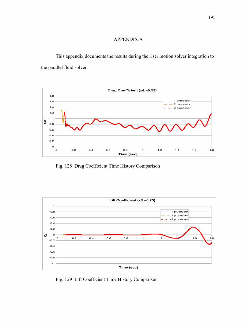
195
APPENDIX A
This appendix documents the results during the riser motion solver integration to
the parallel fluid solver.
Drag Coefficient (x/L=0.25)
0
0.2
0.4
0.6
0.8
1
1.2
1.4
1.6
1.8
0 0.2 0.4 0.6 0.8 1 1.2 1.4 1.6 1.8
Time (sec)
Cd
1 processor
2 processor
3 processor
Fig. 128 Drag Coefficient Time History Comparison
Lift Coefficient (x/L=0.25)
-1
-0.8
-0.6
-0.4
-0.2
0
0.2
0.4
0.6
0.8
1
0 0.2 0.4 0.6 0.8 1 1.2 1.4 1.6 1.8
Time (sec)
CL
1 processor
2 processor
3 processor
Fig. 129 Lift Coefficient Time History Comparison
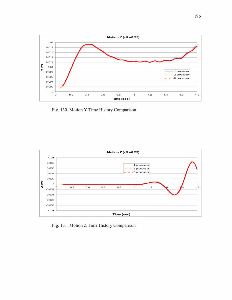
196
Motion Y (x/L=0.25)
0
0.002
0.004
0.006
0.008
0.01
0.012
0.014
0.016
0.018
0.02
0 0.2 0.4 0.6 0.8 1 1.2 1.4 1.6 1.8
Time (sec)
Y (m)
1 processor
2 processor
3 processor
Fig. 130 Motion Y Time History Comparison
Motion Z (x/L=0.25)
-0.01
-0.008
-0.006
-0.004
-0.002
0
0.002
0.004
0.006
0.008
0.01
0 0.2 0.4 0.6 0.8 1 1.2 1.4 1.6 1.8
Time (sec)
Z (m)
1 processor
2 processor
3 processor
Fig. 131 Motion Z Time History Comparison

197
CPU Time Comparison
0%
10%
20%
30%
40%
50%
60%
70%
80%
90%
100%
1 2 3
Processor Number
CPU Time %
Fig. 132 Normalized Computational Time
CF Motion rms a/D (U=0.42m/s)
0.0
0.1
0.2
0.3
0.4
0.5
0.6
0.7
0.8
0.9
0 0.2 0.4 0.6 0.8 1x/L
rms a/D
Test 1105
CFD (FANS serial)
CFD (FANS parallel)
Fig. 133 Cross Flow rms a/D comparison
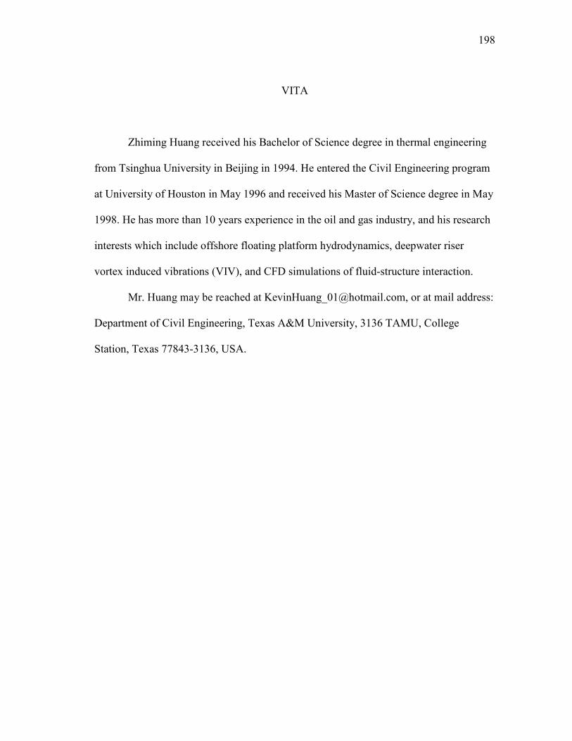
198
VITA
Zhiming Huang received his Bachelor of Science degree in thermal engineering
from Tsinghua University in Beijing in 1994. He entered the Civil Engineering program
at University of Houston in May 1996 and received his Master of Science degree in May
1998. He has more than 10 years experience in the oil and gas industry, and his research
interests which include offshore floating platform hydrodynamics, deepwater riser
vortex induced vibrations (VIV), and CFD simulations of fluid-structure interaction.
Mr. Huang may be reached at [email protected], or at mail address:
Department of Civil Engineering, Texas A&M University, 3136 TAMU, College
Station, Texas 77843-3136, USA.


