

CIRJE Discussion Papers can be downloaded without charge from:
http://www.e.u-tokyo.ac.jp/cirje/research/03research02dp.html
Discussion Papers are a series of manuscripts in their draft form. They are not intended for
circulation or distribution except as indicated by the author. For that reason Discussion Papers may
not be reproduced or distributed without the written consent of the author.
CIRJE-F-616
Customer Lifetime Value and RFM Data:ACCOUNTING YOUR CUSTOMERS: ONE BY ONE
Makoto AbeUniversity of Tokyo
March 2009

Customer Lifetime Value and RFM Data:
ACCOUNTING YOUR CUSTOMERS: ONE BY ONE
Makoto Abe
Graduate School of Economics
The University of Tokyo
7-3-1 Hongo, Bunkyo-ku
Tokyo 113-0033 JAPAN
TEL & FAX: +81-3-5841-5646
E-mail: [email protected]
March 1, 2009
1
Customer Lifetime Value and RFM Data:
ACCOUNTING YOUR CUSTOMERS: ONE BY ONE
ABSTRACT
A customer behavior model that permits the estimation of customer lifetime value (CLV)
from standard RFM data in “non-contractual” setting is developed by extending the
hierarchical Bayes (HB) framework of the Pareto/NBD model (Abe 2008). The model relates
customer characteristics to frequency, dropout and spending behavior, which, in turn, is linked
to CLV to provide useful insight into acquisition. The proposed model (1) relaxes the
assumption of independently distributed parameters for frequency, dropout and spending
processes across customers, (2) accommodates the inclusion of covariates through
hierarchical modeling, (3) allows easy estimation of latent variables at the individual level,
which could be useful for CRM, and (4) provides the correct measure of errors. Using FSP
data from a department store and a CD chain, the HB model is shown to perform well on
calibration and holdout samples both at the aggregate and disaggregate levels in comparison
with the benchmark Pareto/NBD-based model.
Several substantive issues are uncovered. First, both of our datasets exhibit correlation
between frequency and spending parameters, violating the assumption of the existing
Pareto/NBD-based CLV models. Direction of the correlation is found to be data dependent.
Second, useful insight into acquisition is gained by decomposing the effect of change in
covariates on CLV into three components: frequency, dropout and spending. The three
components can exert influences in opposite directions, thereby canceling each other to
produce less effect as the total on CLV. Third, not accounting for uncertainty in parameter
estimate can cause large bias in measures, such as CLV and elasticity. Its ignorance can
potentially have a serious consequence on managerial decision making.
Keywords: CRM, Acquisition, hierarchical Bayes, Pareto/NBD, MCMC

2
1. INTRODUCTION
Customer lifetime value (CLV) is one of the most important concepts in customer
relationship management (CRM). To compute CLV, a customer retention rate, often denoted
as r (Berger and Nasr 1998; Hughes 2000; Jain and Singh 2002), is required. Under
“contractual” setting, customer dropout is clear, and therefore, the retention rate can be
computed easily. Under “non-contractual” setting, however, the timing of customer dropout is
not obvious. Customers do not declare the fact that they become inactive, but simply stop
conducting business with the firm. This situation is also referred to as “unobserved customer
attrition” by Blattberg, Kim and Neslin (2008). So, without knowing customer dropout (and
hence the retention rate) in “non-contractual” setting, how do we compute CLV?
While scoring models work well in practice, Colombo and Jiang (1999) point out the
weakness of scoring models as (1) falling short on generating explanatory insight and (2)
treating customer heterogeneity as noise. Fader, Hardie and Lee (2005) (hereafter referred to
as FHL) describe the problems associated with scoring models when estimating CLV: (1) they
ignore periods 3, 4, 5, failing to capture the dynamics of buyer behavior well into the future,
(2) data must be split into two or more periods in order to calibrate the model, and (3) they
fail to recognize that different “slices” of the data will yield different values of the behavior
variables, resulting in different parameter estimate. Malthouse and Blattberg (2005) report the
difficulty of predicting CLV with scoring models by asserting the 20-55 and 80-15 rules: (1)
of the future top 20% customers, approximately 55% will be misclassified, and (2) of the
future bottom 80%, approximately 15% will be misclassified. The disappointing predictive
accuracy is exacerbated by the fact that their scoring models include a highly flexible (in the
sense of nonlinearity) neural network. These studies seem to imply that a fruitful direction for
estimating CLV in “non-contractual” setting is to construct a probability model based on a
sound behavior theory.

3
A popular approach along this direction is to use a Pareto/NBD model (Schimittlein,
Morrison and Colombo 1978, hereafter referred to as SMC), whereby a customer being
“alive” or “dead” is inferred from recency-frequency data through simple assumptions on
purchase behavior. Some of the CLV research that utilize a Pareto/NBD model include FHL,
Reinartz and Kumar (2003), and Smittlein and Peterson (1994).
The objectives of this research are two folds. First, in light of the previous argument, we
attempt to estimate CLV in “non-contractual” setting with a Pareto/NBD-based behavior
model using only standard recency, frequency, and monetary-value (RFM) data. We limit our
focus on standard RFM data, because RFM analysis is used extensively in industry, implying
that rather rich information on a customer is condensed into these three simple statistics. Even
if firms may not keep the entire purchase history of each customer, most firms in CRM collect,
at least, their customers’ RFM data. The second objective is to obtain useful implications for
prospective customers, as CLV often includes the notion of not only retention but also
acquisition (Berger and Nasr 1998; Blattberg and Deighton 1995, Blattberg, Getz and Thomas
2001). To seek insight into acquisition from the analysis of existing customers, some customer
characteristics (e.g., demographics) are used to relate to RFM data (behavior), and hence CLV.
1.1. Conceptualization of the Model
While the detail will be discussed in the next section, Table 1 highlights our methodology
in comparison with that of SP and FHL. For recency-frequency data, both SP and FHL adopt a
Pareto/NBD model that presumes Poisson purchase and random dropout (a constant hazard
rate) processes whose parameters are independently distributed as gamma. For
monetary-value data, SP posit a normal-normal model, whereby purchase amounts on
different occasions within a customer is normally distributed with the mean following a
normal distribution in order to capture customer heterogeneity. FHL use a gamma-gamma
model, whereby the normal distributions within and across customers in SP are replaced by

4
gamma distributions. Both methodologies can be characterized as an individual-level behavior
model whose parameters are compounded with a mixture distribution to capture customer
heterogeneity, which, in turn, is estimated by an empirical Bayes method. An empirical Bayes
method, in general, utilizes MLE for population-level parameters of the mixture distribution,
which specifies the prior for individual-level parameters that are updated in a Bayesian
manner.
-------------------------------- Insert Table 1 about here.
--------------------------------
The proposed methodology posits the same behavioral assumptions as SP and FHL, yet
customer heterogeneity is captured through a more general mixture distribution to account for
dependence among the three behavior processes: purchase, dropout, and spending. Our
approach extends the Hierarchical Bayes framework of the Pareto/NBD model on customer
transaction (Abe 2008) to purchase amount, whereby (1) the analytical part of the
heterogeneity mixture distribution is replaced by a simulation method, and (2) unobservable
measures, such as a customer lifetime (survival) and an active/inactive indicator, are
incorporated into the model as latent variables. By avoiding analytical aggregation, the
approach leads to a simpler and cleaner model that offers various advantages.
First, the proposed model relaxes the assumption of independently distributed parameters,
λ, μ, and η, respectively, for purchase, dropout, and spending processes across customers,
which is made in the Pareto/NBD with normal-normal (SP) or gamma-gamma (FHL)
spending model. Managerially, this assumption restricts that shopping frequency, lifetime, and
spending per trip are not related. One might speculate certain relationship, for instance,
frequent shoppers tend to live longer and/or spend higher amounts (Reinartz, Thomas and
Kumar 2005; Thomas, Reinartz and Kumar 2003). The proposed HB model accommodates a
more general correlated mixture distribution with ease, because aggregation of heterogeneous

5
customers is carried out by a simulation method. In the empirical section, we will indeed find
that models by SP and FHL should not be applied to both of our datasets since the
independence assumption does not hold. Our method not only accommodates correlation
among parameters, but also allows the performing of statistical inference on the independence
assumption.
Second, hierarchical models, whereby customer-specific parameters, λ, μ, and η, are a
function of covariates, can be constructed and estimated with ease.
(a) This implies that, even in the absence of RFM data, customer characteristics can be used to
predict purchase, dropout, and spending behavior, and thus CLV to certain extent.
Operationally, such models can be quite useful when seeking prospective customers with
high CLV for acquisition.
(b) Substantively, such hierarchical models can shed light on interesting yet conflicting
findings in CRM. For example, what are characteristics of loyal (long lifetime) customers,
and whether loyal customers spend more? Previous research investigated such issues with
a two-step approach: lifetime duration is first estimated to identify loyal customers, and
then customer characteristics (explanatory variables) are related to the lifetime duration
(dependent variable). A hierarchical model, whose dropout parameter is a function of
customer characteristics, can be estimated in one step, providing the correct measure of
error for statistical inference.
Third, in the HB model, posterior distributions of purchase rate λ, dropout rate μ, and
spending parameter η are constructed at the individual level by MCMC draws as a byproduct
of the estimation. Thus, any of their statistics, such as mean and variance, can be computed by
simple algebra, as discussed in Abe (2008).1 It is also straightforward to obtain a distribution
1 In a Pareto/NBD model, the expressions for the posterior density of an individual level λ, μ, and η involve complicated integration that cannot be reduced. Furthermore, as a new statistic based on λ, μ, and η is required (such as a mean, a variance, a survival probability, the

6
of any individual statistic that is a function of λ, μ, and η, such as a survival probability and
CLV, by evaluating the function for each MCMC draw of λ, μ, and η. For this reason, the
model provides useful individual level information for CRM, such as ranking customers
according to frequency, lifetime, spending, CLV, etc.
Forth, a Bayesian framework using MCMC simulation provides a posterior distribution
of parameters being estimated rather than point estimate, thereby providing a correct measure
of error necessary for statistical inference, even with a small sample. It also has advantage
over the Pareto/NBD-based model estimated by empirical Bayes, which overestimates the
precision because the same data is used twice, once for constructing the likelihood function
describing customer specific behavior and the other for estimating the prior (mixture
distribution). It will be shown that ignoring uncertainty can lead to biased statistics such as
CLV, and therefore, resulting in incorrect managerial decisions.
In the next section, the proposed HB model is described and compared against the
Pareto/NBD-based model, followed by an explanation of the model estimation using an
MCMC method in conjunction with a data augmentation technique. Then, empirical analyses
using data from frequent shopper program of a department store and a music CD chain is
presented. Finally, conclusions and future directions are discussed.
2. PROPOSED MODEL OF CLV
2.1. Model Assumptions
This section describes the assumptions of the HB model.
Individual Customer
expected number of transaction and CLV), an analytical expression must be derived each time from the posterior distributions of λ, μ, and η. In actual computation, numerical evaluation of this integration (i.e., non-standard hypergeometric function of various kinds) must be repeated for each statistic and for each customer. This makes the computation of the individual level statistics difficult in Pareto/NBD models.

7
Assumption 1: Poisson purchases. While active, each customer makes purchases according to
a Poisson process with rate λ.
Assumption 2: Exponential lifetime. Each customer remains active for a lifetime, which has
an exponentially distributed duration with dropout rate μ.
Assumption 3: Lognormal spending. Within each customer, amounts of spending on purchase
occasions are distributed as lognormal with location parameter η.
Assumptions 1 and 2 are identical to the behavioral assumptions of a Pareto/NBD model.
Because their validity has been studied by other researchers (FHL 2005; Reinartz and Kumar
2000, 2003; SMC 1987; SP 1994), justification is not provided here for brevity. Assumption 3
is specified because (1) the domain of spending is positive, and (2) inspection of the
distributions of spending amounts within customers reveals a skewed shape resembling
lognormal. As described previously, SP and FHL assume normal and gamma, respectively, to
characterize the distribution of spending amounts within a customer.
Heterogeneity across Customers
Assumption 4: Individuals’ purchase rates λ, dropout rates μ, and spending parameters η
follow a multivariate lognormal distribution.
Assumption 4 permits correlation among purchase, dropout, and spending parameters.
Because Assumption 4 implies that log(λ), log(μ), and log(η) follow a multivariate normal,
estimation of the variance-covariance matrix is tractable using a standard Bayesian method. A
Pareto/NBD combined with either normal-normal (SP) or gamma-gamma (FHL) spending
model posits independence among the three behavioral processes. Both SP and FHL
acknowledge the restriction on their models and perform an extensive assumption check on
their data to validate their application.

8
2.2. Mathematical Notations
For recency and frequency data, we will follow the standard notations {x, tx, T}, used by
SMC, FHL, and Abe (2008). τ is an unobserved customer lifetime. For spending, s denotes
the amount of spending on a purchase occasion. Using these mathematical notations, the
previous assumptions can be expressed as follows.
(1) .210
if !)(
if !)(
]|[
,.,, x
Tex
TexT
xP x
T
x
=
⎪⎪⎩
⎪⎪⎨
⎧
≤
>=
−
−
τλτ
τλ
λτλ
λ
(2) 0 )( ≥= − τμτ τμef
(3) 0 ) ,)(log(~log(s) 2 >sN ωη
(4) ⎟⎟⎟⎟
⎠
⎞
⎜⎜⎜⎜
⎝
⎛
⎥⎥⎥
⎦
⎤
⎢⎢⎢
⎣
⎡
=Γ⎥⎥⎥
⎦
⎤
⎢⎢⎢
⎣
⎡=
⎥⎥⎥
⎦
⎤
⎢⎢⎢
⎣
⎡
2
2
2
00 ,~)log()log()log(
ηημηλ
μημμλ
ληλμλ
η
μ
λ
σσσσσσσσσ
θθθ
θημλ
MVN
where N and MVN denote univariate and multivariate normal distributions, respectively. ω2 is
the variance of spending amounts within a customer.
2.3. Expressions for Transactions, Sales, and CLV
Given the individual level parameters for (λ, μ), the expected number of transactions in
the time period of u, E[X(u)|λ, μ], becomes
(5) ( ) ),min( here w1][],|)([ ueEuXE u τψμλψλμλ μ =−== − .
The expected sales during this period u is simply the product of the expected number of
transactions shown in Equation (5) and the expected spending E[s] as
(6) ( )ueeuXEsEusalesE μω
μλημλωηωημλ −−== 1],|)([],|[],,,|)([ 2/2
.
9
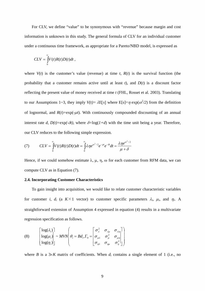
For CLV, we define “value” to be synonymous with “revenue” because margin and cost
information is unknown in this study. The general formula of CLV for an individual customer
under a continuous time framework, as appropriate for a Pareto/NBD model, is expressed as
∫∞
=0
)()()( dttDtRtVCLV ,
where V(t) is the customer’s value (revenue) at time t, R(t) is the survival function (the
probability that a customer remains active until at least t), and D(t) is a discount factor
reflecting the present value of money received at time t (FHL, Rosset et al. 2003). Translating
to our Assumptions 1~3, they imply V(t)= λΕ[s] where E[s]=η exp(ω2/2) from the definition
of lognormal, and R(t)=exp(-μt). With continuously compounded discounting of an annual
interest rate d, D(t)=exp(-δt), where δ=log(1+d) with the time unit being a year. Therefore,
our CLV reduces to the following simple expression.
(7) δμ
ληληω
δμω
+=== ∫∫
∞−−
∞ 2/
0
2/
0
22
)()()( edteeedttDtRtVCLV tt
Hence, if we could somehow estimate λ, μ, η, ω for each customer from RFM data, we can
compute CLV as in Equation (7).
2.4. Incorporating Customer Characteristics
To gain insight into acquisition, we would like to relate customer characteristic variables
for customer i, di (a K×1 vector) to customer specific parameters λi, μi, and ηi. A
straightforward extension of Assumption 4 expressed in equation (4) results in a multivariate
regression specification as follows.
(8) ⎟⎟⎟⎟
⎠
⎞
⎜⎜⎜⎜
⎝
⎛
⎥⎥⎥
⎦
⎤
⎢⎢⎢
⎣
⎡
=Γ=⎥⎥⎥
⎦
⎤
⎢⎢⎢
⎣
⎡
2
2
2
0
i
,~)log()log()log(
ηημηλ
μημμλ
ληλμλ
σσσσσσσσσ
θημλ
ii
i
i BdMVN
where B is a 3×K matrix of coefficients. When di contains a single element of 1 (i.e., no

10
characteristic variables), the common mean, θ0=θi for all customers i, is estimated.
2.5. Elasticities
Useful implications can be obtained from computing elasticities of CLV with respect to
(a) λ, μ, and η, and (b) characteristic variables di. From equation (7),
(9) 1//
=∂
∂=
λλλCLVCLVECLV ,
δμμ
μ +−=CLVE , 1=CLVEη ,
implying that one percent increase in the purchase rate or spending parameter causes one
percent increase in CLV, whereas one percent decrease in the dropout rate leads to less than
one percent increase in CLV with the magnitude depending on the discount rate δ. Under a
high interest rate, the impact of prolonging lifetime on CLV is not as rewarding since future
customer value would be discounted heavily.
The effect of customer characteristics on CLV can be decomposed into frequency,
dropout, and spending processes to provide further insight. Defining dik as the k-th
(continuous) characteristic of customer i, the elasticity becomes
(10)
CLVd
CLVd
CLVdikk
i
ikk
i
ik
ik
i
i
i
ik
i
i
i
ik
i
i
i
ikik
iiCLVd
ikikik
ik
EsEdEfdbb
b
CLVd
dCLV
dCLV
dCLV
ddCLVCLVE
++=⎥⎦
⎤⎢⎣
⎡+
+−=
⎥⎦
⎤⎢⎣
⎡∂∂
∂∂
+∂∂
∂∂
+∂∂
∂∂
=∂
∂=
ημ
λ δμμ
ηη
μμ
λλ/
/
where blk (l∈{λ,μ,η}, k=1,..,K) denotes (l, k)th element of matrix B.
3. ESTIMATION
In the previous section, analytical expressions for the customer process of frequency,
dropout, and spending, are derived from the basic behavioral Assumptions 1, 2, and 3. To
account for customer heterogeneity, the HB approach does not require the aggregate analytical
expressions compounded by the mixture distribution.
3.1. Estimation of the Transaction (RF) Component

11
The transaction component is identical to the HB extension of the Pareto/NBD model
proposed by Abe (2008). It is estimated by MCMC simulation through a data augmentation
method. Because information about customer i being active (zi=1) or not at time T, and if not,
the dropout time ( yi<Ti ) is unknown, zi and yi are considered as latent variables, which are
randomly drawn from their posterior distributions. The detail is described in Abe.
3.2. Estimation of the Spending (M) Component
As explained at the beginning of this paper, we limit our behavior data to recency,
frequency, and monetary-value (RFM), so that the model can be implemented even if a firm
does not keep the complete purchase history of each customer. The RFM data for customer i
are denoted as (xi, txi, Ti, asi), where xi, txi and Ti are defined as in SMC and asi stands for
average spending per purchase occasion. Without the knowledge of spending variation within
a customer from one purchase to another, however, there is no means to infer the variance of
logarithmic spending ω2, specified in equation (3), from RFM data alone. Here, we assume
that ω2 is known (for example, from past data) and common across customers.2
Assumption 3 allows adoption of standard normal conjugate updating in Bayesian
estimation, whereby the posterior mean is a precision weighted average of the sample and the
prior means. For this method to work, however, we need the mean of log(spending)s (or
equivalently, the logarithm of the geometric mean of spending amounts) from each customer,
whereas the M part of RFM data provides only the arithmetic mean of spendings asi. The
appendix shows that the sample mean of log(spending)s, can be approximated by the average
spending asi and ω2, as in Equation (11).
2 To characterize variation in spending, we could have assumed that either ω2, the variance in logarithmic spending, or the variance in the natural scale of spending is known. We posited the former because it seemed more reasonable to think that the magnitude of spending variation grows as the spending level increases, and inspection of the data supported our speculation.
12
(11) ⎟⎟⎠
⎞⎜⎜⎝
⎛+−≅∑
= 421)log()log(1 4
2
1
ωωi
x
mim
i
assx
i
3.3. Prior Specification
Let us denote the customer specific parameters as ϕi = [ log(λi), log(μi) log(ηi) ]’, which
is normally distributed with mean θi=Bdi and variance-covariance matrix Γ0 as in Equation (8).
Our objective is to estimate parameters { ϕi, yi, zi, ∀i; Β, Γ0} from observed RFM data {xi, txi,
Ti, asi; ∀i}. In the HB framework, the prior of individual-level parameter ϕi corresponds to
the population distribution MVN(Bdi, Γ0). The priors for the hyperparameters B and Γ0 are
chosen to be multivariate normal and inverse Wishart, respectively.
( )0000 ,~)( ΣbMVNBvec , ( )00000 ,~ ΓΓ νIW
These distributions are standard conjugate priors for multivariate regression models.
Constants (b00, Σ00, ν00, Γ00) are chosen to provide very diffuse priors for the hyperparameters.
3.4. MCMC Procedure
We are now in a position to estimate parameters { ϕi, yi, zi, ∀i; Β, Γ0} using an MCMC
method. To estimate the joint density, we sequentially generate each parameter, given the
remaining parameters, from its conditional distribution until convergence is achieved. The
algorithm can be found in Abe (2008).
4. EMPIRICAL ANALYSIS
4.1. FSP data for a department store
We now apply the proposed model to real data. The first dataset contains shopping
records for 400 members of a frequent shopper program (FSP) at a department store in Japan.
The first and the second 26 weeks of the data are used for model calibration and validation,
respectively. They are the same data used by Abe (2008), and their detail can be found in his

13
paper. As discussed in Section 3.1, the variance of log(spending)s within customers, ω2, is
assumed to be known. It was estimated to be 0.895 from the calibration data.
4.1.1. Model Validation
The MCMC steps were put through 15,000 iterations, of which the last 5,000 were used
to construct the posterior distribution of parameters. The convergence was monitored visually
and checked with the Geweke test (Geweke 1992). The dispersion of the proposal distribution
in the Metropolis-Hastings algorithm was chosen such that the acceptance rate stayed at about
40% to allow even drawing from the probability space (Gelman et al. 1995).
-------------------------------- Insert Table 2 about here.
--------------------------------
Table 2 shows the result of various models that include different covariates. Before
attempting to interpret the result, let us first discuss the model validation focusing on Model 3,
which has the best marginal loglikelihood, as shown in the last row. The performance of
Model 3 was evaluated with respect to the number of transactions and spending, obtained
from Equations (5) and (6), respectively, in comparison with the benchmark
Pareto/NBD-based model. The expected number of transactions, predicted by the Pareto/NBD,
was multiplied by his/her average spending asi to come up with customer i’s spending.
-------------------------------- Insert Figure 1 about here. --------------------------------
Figure 1 shows the time-series tracking for the cumulative number of repeat purchases.
Both models provide good fit in calibration and forecast in validation, which are separated by
the vertical dashed line. With respect to the mean absolute percent errors (MAPE) between
predicted and observed weekly cumulative purchases, the HB model performed better for
validation (1.3% vs. 1.9%) and comparable for calibration (2.5% vs. 2.5%).
-------------------------------- Insert Table 3 about here.

14
--------------------------------
Fit statistics at the disaggregate level provide more stringent performance measures.
Table 3 compares the correlation and mean squared error (MSE) between prediction and
observation with respect to the number of transactions and total spending at the individual
customer level during calibration and validation periods. While both models offer similar
performance, the HB is slightly superior in predicting spending.
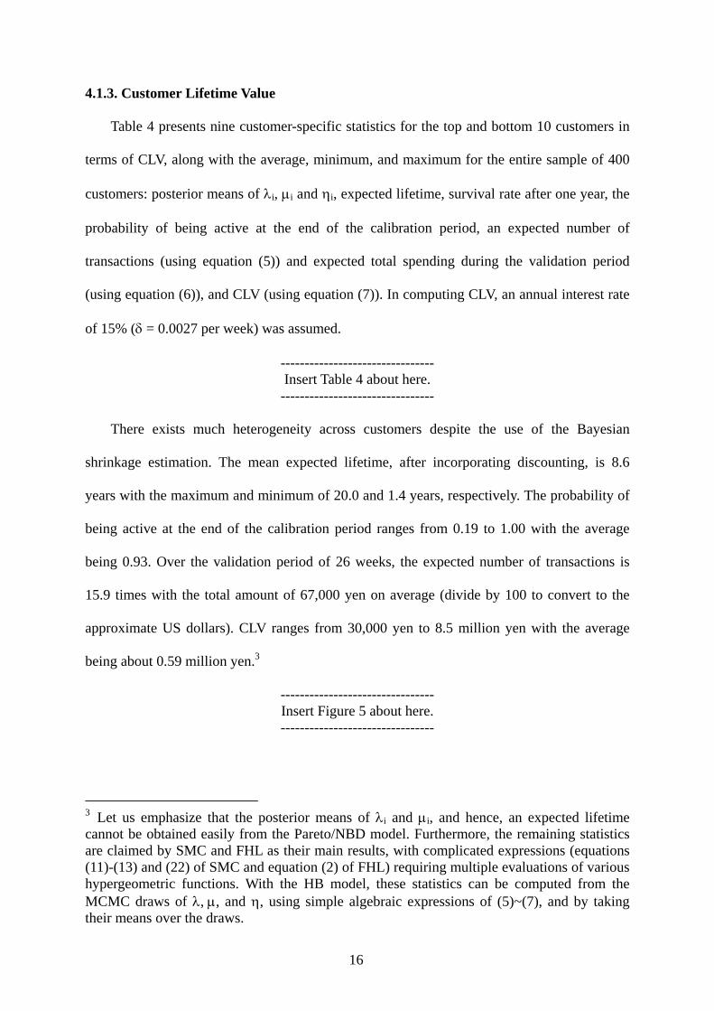
-------------------------------- Insert Figures 2 and 3 about here.
--------------------------------
Figure 2 shows the predicted number of transactions during the validation period,
averaged across individuals, conditional on the number of purchases made during the
calibration period. Figure 3 compares the predicted total spending during the validation period
in the similar manner. Both figures demonstrate the superiority of the HB model over the
Pareto/NBD-based model visually.
In sum, the HB model seems to fit and predict well in comparison with the
Pareto/NBD-based model, in terms of the number of transactions and spending both at the
aggregate and disaggregate levels. However, the difference of the two models is minor.
4.1.2. Interpretation of the Model Estimation
Having established the validity of the HB model, let us now examine Table 2 to interpret
the estimation result. FOOD, the fraction of store visits on which food items were purchased
and a proxy for store accessibility, is the most important covariate with the significant positive
and negative coefficients for log(λ) and log(η), respectively, at the 5% level. The result is also
supported by the Pareto/NBD model of Abe (2008), whereby “average spending” covariate
was found to be significantly negative for log(λ). Managerially, food buyers tend to shop
more often and spend a smaller amount on each shopping trip. This finding is consistent with
the story told by a store manager in that, although food buyers spend a smaller amount on
15
each shopping trip, they visit the store often enough to be considered as vital. Another
significant covariate is AGE for log(η), implying that older customers tend to spend more at
each shopping trip. This is hardly surprising either. Older people with lower income would
shop in discount stores close to where they live rather than venture out or bother to visit a
department store located in a busy shopping district, like this retailer.
Let us now turn our attention to the relationship among purchase rate λ, dropout rate μ,
and spending parameter η. To check whether the independence assumption of Pareto/NBD is
satisfied, correlation of Γ0 must be tested on the intercept-only model (Model 0) but not the
covariate model. This is because, if covariates explain the correlation among λ, μ and
η completely, then no correlation remains in the error term as captured by Γ0. First, we see
that the correlation between log(λ) and log(μ) is not significantly different from 0, implying
that the assumption of Pareto/NBD holds here. Second, correlation between log(λ) and
log(η) is significantly negative (-0.28), the fact that is consistent with the FOOD variable
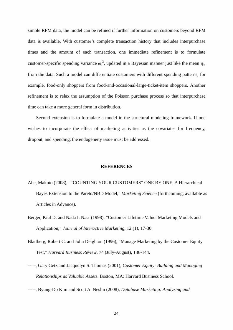
having opposite signs on log(λ) and log(η) in Model 3. Figure 4 presents the scatter plot of
the mean values of the individual λi and ηi (i=1,..,400). One can visually observe the
correlation.
-------------------------------- Insert Figure 4 about here. --------------------------------
Hence, the assumption of the independence between transaction (RF) and spending (M)
components in the Pareto/NBD based model (SP and FHL) is violated in this dataset. For
researchers using the SP and FHL models, the finding emphasizes the importance of verifying
the independent assumption (as was done in SP and FHL). Managerially, this negative
correlation implies that a frequent shopper tends to spend a smaller amount on each trip. No
correlation is found between shopping frequency and his/her lifetime or between lifetime and
per-trip spending.
16
4.1.3. Customer Lifetime Value
Table 4 presents nine customer-specific statistics for the top and bottom 10 customers in
terms of CLV, along with the average, minimum, and maximum for the entire sample of 400
customers: posterior means of λi, μi and ηi, expected lifetime, survival rate after one year, the
probability of being active at the end of the calibration period, an expected number of
transactions (using equation (5)) and expected total spending during the validation period
(using equation (6)), and CLV (using equation (7)). In computing CLV, an annual interest rate
of 15% (δ = 0.0027 per week) was assumed.
-------------------------------- Insert Table 4 about here.
--------------------------------
There exists much heterogeneity across customers despite the use of the Bayesian
shrinkage estimation. The mean expected lifetime, after incorporating discounting, is 8.6
years with the maximum and minimum of 20.0 and 1.4 years, respectively. The probability of
being active at the end of the calibration period ranges from 0.19 to 1.00 with the average
being 0.93. Over the validation period of 26 weeks, the expected number of transactions is
15.9 times with the total amount of 67,000 yen on average (divide by 100 to convert to the
approximate US dollars). CLV ranges from 30,000 yen to 8.5 million yen with the average
being about 0.59 million yen.3
-------------------------------- Insert Figure 5 about here. --------------------------------
3 Let us emphasize that the posterior means of λi and μi, and hence, an expected lifetime cannot be obtained easily from the Pareto/NBD model. Furthermore, the remaining statistics are claimed by SMC and FHL as their main results, with complicated expressions (equations (11)-(13) and (22) of SMC and equation (2) of FHL) requiring multiple evaluations of various hypergeometric functions. With the HB model, these statistics can be computed from the MCMC draws of λ, μ, and η, using simple algebraic expressions of (5)~(7), and by taking their means over the draws.

17
Figure 5 shows a gain chart (solid line), in which customers are sorted according to the
decreasing order of CLV and the cumulative CLV (y-axis, where the total CLV is normalized
to 1) is plotted against the number of customers (x-axis). In addition, two gain charts are
plotted. The dash-dotted line is based solely on recency criterion, whereby customers are
sorted in the order of increasing recency (from most recent to least recent). The dotted line is
a gain chart based on customers being ordered according to the sum of the three rankings of
recency, frequency and monetary value. The 45 degree dashed line corresponds to the
cumulative CLV for randomly ordered customers. This figure implies that recency criterion
alone is not sufficient to identify good customers, despite many companies use this criterion.
On the other hand, combined use of the three criteria (recency, frequency and monetary-value),
even with the naïve equal weighting scheme, seems to provide rather accurate ordering of
CLV. This finding strongly supports the wide use of RFM analysis and regression-type
scoring models among practioners for identifying good customers.
4.1.4. Elasticity of Covariates on CLV
Another advantage of our Bayesian approach is that these statistics reflect the uncertainty
in parameter estimates. Ignoring their uncertainty and computing various statistics from their
point-estimates, say MLE, as if parameters are deterministic, could produce biased result,
leading to incorrect managerial decisions. The point is illustrated in Table 5, which shows the
decomposition of the elasticity of CLV with respect to each covariate into frequency, dropout,
and spending components. To account for parameter uncertainty, elasticity is computed for
each set of the 5000 MCMC draws of blk and μi according to Equation (10), which is then
averaged over the 5000 draws and 400 customers. When the posterior mean of blk and μi is
directly substituted into Equation (10) (bottom table) instead of averaging over MCMC draws
(top table), elasticity with respect to the dropout component is overestimated (because of
nonlinearity in μi), even if customer heterogeneity is accounted for.

18
-------------------------------- Insert Table 5 about here.
--------------------------------
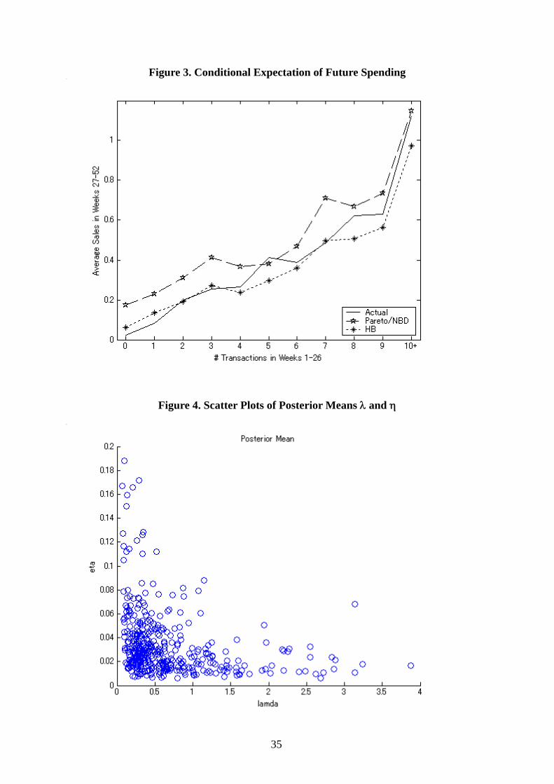
To visualize the impact of covariates, the solid line in Figure 6 plots the value of
log(CLV) for different values of a covariate when the other two covariates are fixed at their
mean values. These graphs are computed using the mean estimate of the coefficients of Model
3 shown in Table 2, assuming that all covariates are continuous. For the FEMALE covariate,
therefore, it should be interpreted as how log(CLV) varies when the gender mixture is
changed from the current level of 93.3% female, while keeping the other two covariates
unchanged. The dotted vertical line indicates the mean value of the covariate under
consideration. Both FOOD and AGE have strong influences on log(CLV), whereas FEMALE
exerts a very weak influence.
-------------------------------- Insert Figure 6 about here. --------------------------------
Figure 6 also attempts to decompose the influence of covariates on log(CLV) into three
components: frequency, dropout and spending. Taking logarithm of the basic formula of CLV
in Equation (7) results in the following summation expression.
[ ] [ ] [ ]
[ ] [ ] [ ] 'component Spending componentFrequency componentDropout
')log()log()log(
2/)log()log()log()log( 2
c
cccc
CLV
sfd
+++=
+++++++−=
++++−=
ηλδμ
ωηλδμ
The graph can be interpreted as stacking these three components, dropout, frequency, and
spending, from top to bottom, to constitute the overall log(CLV). To account for the scale
differences among these components, cd, cf, and cs are chosen such that each component is
normalized to 1 at the mean value of the covariate. Therefore, log(CLV)=3 at the dotted
vertical line.
The direction and magnitude of the effect of each covariate on the three components are

19
consistent with the signs of the posterior means blk (l∈{λ,μ,η}, k=1,..,K). Increasing the
fraction of food buyers improves dropout (lengthen lifetime) and frequency, but decreases
spending per trip with net increase in the overall CLV. Increasing the fraction of elderly
people increases the spending without much influence on dropout and frequency, thereby
resulting in net increase in the overall CLV. Increasing the fraction of female leads to little
improvement in all three components and, hence, a negligible increase in the overall CLV.
Elasticity decomposition, shown in Figure 6 and Table 5, provides managers with useful
insight into acquisition. An effort to manipulate certain customer characteristics might impact
dropout, frequency, and spending components in opposite directions, thereby canceling each
other to produce less effect as the total on CLV. For example, much of the improvement in
frequency, from increasing the fraction of food buyers, is negated by the decline in spending,
and only the dropout improvement provides the net contribution to CLV, as can be seen from
Table 5 and the near flat dashed line of Figure 6. On the other hand, an effort to increase the
proportion of elderly people is met with the boost in CLV, due to increased spending per trip
with only a small negative influence on frequency.
To build effective acquisition strategy from these results, managers must make a fine
balance between desired customer characteristics (i.e., demographics), desired behavioral
profiles (i.e., dropout, frequency, and spending), responsiveness (elasticity) of the
characteristic covariates on CLV, and acquisition cost of the desired target customers.
4.2. Retail FSP data for a Music CD chain
The second dataset is obtained from a FSP of a large chain for music CD. These data are
also identical to the one used by Abe (2008). As for the first dataset, the MCMC steps were
repeated 15,000 iterations and the last 5,000 were used to construct posterior distributions.
Table 6 compares the performance of HB against Pareto/NBD for the number of transactions
and spending at the customer level. The HB model is slightly superior to the Pareto/NBD in

20
all criteria, and the visual plots, like Figures 2 and 3 shown for the department store, also
confirm the fact.
-------------------------------- Insert Tables 6 and 7 about here.
--------------------------------
Table 7 reports the model estimation. Let us first examine Model 3, which results in the
highest marginal loglikelihood, for significant explanatory variables. First, the amount of an
initial purchase is positively significant on log(λ) and log(η), implying that customers with a
larger trial purchase tend to buy more frequently and spend more per trip in the subsequent
repeat purchases. Second, older customers appear to spend more per shopping trip.
Next, we turn our attention to the intercept model Model 0 for the relationship among λ,
μ, and η. First, we see that the correlation between log(λ) and log(μ) is not significantly
different from 0, implying that the assumption of Pareto/NBD holds here. Second, correlation
between log(λ) and log(η) is significantly positive (0.14), the fact that is consistent with the
initial purchase variable having the same significant signs on log(λ) and log(η). Once again,
the independence assumption of the transaction and spending components in the Pareto/NBD
based model (SP and FHL) is violated. This time, however, the sign is in the opposite
direction, implying that the correlation between purchase frequency and spending per
occasion is context dependent. While not the “average spending”, it is consistent with the
Pareto/NBD model of Abe (2008) whereby “initial purchase amount” covariate has a
significant positive sign for log(λ). Managerially, the correlation implies that frequent buyers
spend more per shopping occasion.
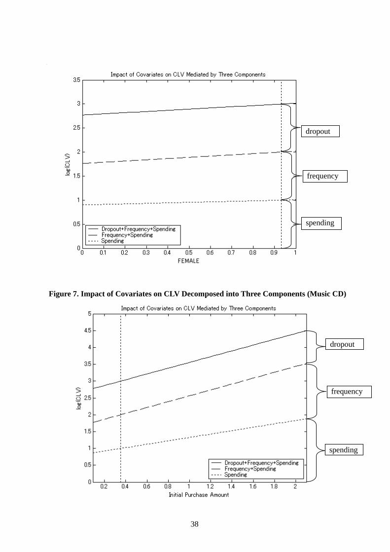
-------------------------------- Insert Table 8 and Figure 7 about here.
--------------------------------
Table 8 shows the elasticity decomposition of CLV into frequency, dropout, and spending
components. When parameter uncertainty is not accounted for, the dropout component is

21
overestimated, as was the case for the department store data, by about 20%. Elasticity
decomposition of CLV into the three components for varying levels of the three covariates is
presented in Figure 7. A higher initial purchase amount is related to higher CLV by increasing
frequency and increasing spending with almost no change in dropout. Older customers are
associated with less frequency, reduced dropout, and higher spending per trip with the positive
net contribution to CLV. Female customers are associated with less frequency, less dropout,
less spending with the negative net contribution to CLV.
-------------------------------- Insert Table 9 about here.
--------------------------------
Finally, Table 9 presents nine customer-specific statistics for the top and bottom 10 customers
in terms of CLV, along with the average, minimum, and maximum for the entire sample of
500 customers.
CONCLUSIONS
An individual behavior model that permits the estimation of CLV from standard RFM
data in “non-contractual” setting was developed based on the HB framework. The model also
related customer characteristics to frequency, dropout and spending behavior, which, in turn,
were linked to CLV to provide useful insight into acquisition. The HB model posited three
sound behavioral assumptions from previous research: (1) a Poisson purchase process, (2) a
random dropout process (i.e., exponentially distributed lifetime), and (3) a lognormally
distributed spending process, while accounting for customer heterogeneity in all three
processes. Because, in the HB framework, heterogeneity was captured as a prior rather than
through a mixture distribution, the entire modeling effort could bypass all the complications
associated with aggregation, which was left to MCMC simulation. Using FSP data from a
Japanese department store and a CD chain, the HB model was shown to perform well on

22
calibration and holdout samples both at the aggregate and disaggregate levels in comparison
with the benchmark Pareto/NBD-based model.
Methodological contributions of this research are [1] a development of the
individual-level behavioral model for RFM data in the HB framework, in which an empirical
Bayes approach was used previously, and [2] the MCMC method that combines a data
augmentation technique to permit the estimation of individual level latent variables, such as
an active/inactive indicator and dropout time in our study. The approach offers: (1)
accommodation of correlated parameters, (2) ease of estimating latent variables at the
individual level, (3) extension to hierarchical models incorporating covariates, and (4)
estimation of the correct measure of errors. The proposed methodology has made it possible
to address many issues suggested as future extensions by previous research (Blattberg et al.
2008, p.129; FHL 2005; Jain and Singh 2002; SMC 1987).
In addition, several substantive issues were uncovered.
- The independence between transaction (RF) and spending (M) components could be
violated. Our datasets exhibited weak yet significant correlation between frequency and
spending. Furthermore, the direction of the correlation is data dependent. Researchers must
always check this assumption with their data before applying a Pareto/NBD-based model.
- Effect of the change in covariates on CLV is decomposed into three components: frequency,
dropout and spending. They could have opposite signs, thereby canceling each other to
produce less effect as the total on CLV. In our department store data, much of the
improvement in frequency, from increasing the fraction of food buyers, was negated by the
decline in spending, and only the dropout improvement contributed to the net increase in
CLV.
- Not accounting for uncertainty in parameter estimate can cause bias in statistics, such as
CLV and elasticity in our study, if the expression involving parameters is nonlinear. While

23
marketing has paid the universal attention to accommodating heterogeneity, that is not the
case for parameter uncertainty. When computing elasticity, for example, some researchers
simply substitute point-estimate, such as MLE, into the formula without bothering to
account for their standard errors. Bayesian methods, in conjunction with sampling
estimation techniques, are powerful means to address this uncertainty issue even under small
samples because they do not rely on the asymptotic theories.
Finally, the model provides the following managerial implications when implemented on
a CRM system that collects RFM data.
- The model outputs, besides a customer-specific survival rate, include individual level λi, μi
and ηi, expected lifetime, the probability of being active, expected number of future
transactions, expected total spending, and CLV, some of which would be difficult, if not
impossible, to obtain from the Pareto/NBD-based model. These statistics fully recognize the
difference among customers and can be useful in implementing effective customized
marketing.
- Useful insight into acquisition can be gained from a simple formula of CLV (Equation (7))
and its elasticity decomposition into dropout, frequency, and spending components that are
linked to customer characteristics (Equation (10)).
- When planning managerial actions based on a model, for example, by adding an
optimization module, uncertainty in parameter estimation can easily be incorporated with
the simulation-based MCMC method. Ignoring uncertainty could potentially have a serious
consequence on decision making.
The current study is only the beginning for the stream of research toward understanding
customer behavior in “non-contractual” setting. Possible extensions are synonymous to the
limitations of the current model. First, while our assumption of Poisson purchase (i.e.,
exponentially distributed interpurchase time) and lognormal spending might to be suitable for
24
simple RFM data, the model can be refined if further information on customers beyond RFM
data is available. With customer’s complete transaction history that includes interpurchase
times and the amount of each transaction, one immediate refinement is to formulate
customer-specific spending variance ωi2, updated in a Bayesian manner just like the mean ηi,
from the data. Such a model can differentiate customers with different spending patterns, for
example, food-only shoppers from food-and-occasional-large-ticket-item shoppers. Another
refinement is to relax the assumption of the Poisson purchase process so that interpurchase
time can take a more general form in distribution.
Second extension is to formulate a model in the structural modeling framework. If one
wishes to incorporate the effect of marketing activities as the covariates for frequency,
dropout, and spending, the endogeneity issue must be addressed.
REFERENCES
Abe, Makoto (2008), ““COUNTING YOUR CUSTOMERS” ONE BY ONE; A Hierarchical
Bayes Extension to the Pareto/NBD Model,” Marketing Science (forthcoming, available as
Articles in Advance).
Berger, Paul D. and Nada I. Nasr (1998), “Customer Lifetime Value: Marketing Models and
Application,” Journal of Interactive Marketing, 12 (1), 17-30.
Blattberg, Robert C. and John Deighton (1996), “Manage Marketing by the Customer Equity
Test,” Harvard Business Review, 74 (July-August), 136-144.
-----, Gary Getz and Jacquelyn S. Thomas (2001), Customer Equity: Building and Managing
Relationships as Valuable Assets. Boston, MA: Harvard Business School.
-----, Byung-Do Kim and Scott A. Neslin (2008), Database Marketing: Analyzing and

25
Managing Customers, New York, USA: Springer.
Colombo, Richard and Weina Jiang (1999), “A Stochastic RFM Model,” Journal of Interactive
Marketing, 13 (3), 2-12.
Congdon, Peter (2001), Bayesian Statistical Modelling, London, UK: Wiley.
Fader, Peter S., Bruce G. S. Hardie, and Ka Lok Lee (2005), “RFM and CLV: Using Iso-Value
Curves for Customer Base Analysis,” Journal of Marketing Research, 42 (4), 415-430.
Gelman, Andrew, John B. Carlin, Hal S. Stern, and Donald B. Rubin (1995), Bayesian Data
Analysis, Boca Raton, Florida: Chapman & Hall.
Geweke, J. (1992), “Evaluating the Accuracy of Sampling-Based approaches to the Calculation
of Posterior Moments,” in J. M. Bernardo, J. M. Berger, A. P. Dawid and A. F. M. Smith,
(eds.), Bayesian Statistics 4, 169-193, Oxford: Oxford University Press.
Hughes, Arthur (2000), Strategic Database Marketing (2nd Ed), New York: McGraw-Hill.
Jain, Dipak, and Siddhartha S. Singh (2002), “Customer Lifetime Value Research in Marketing:
A Review and Future Directions,” Journal of Interactive Marketing, 16 (2), 34-46.
Malthouse, Edward C. and Robert C. Blattberg (2005), “Can We Predict Customer Lifetime
Value?” Journal of Interactive Marketing, 19 (1), 2-15.
Reinartz, Werner J. and V. Kumar (2000), “On the Profitability of Long-Life Customers in a
Noncontractual Setting: An Empirical Investigation and Implications for Marketing,”
Journal of Marketing, 64 (4), 17-35.
----- and ----- (2003), “The Impact of Customer Relationship Characteristics on Profitable
Lifetime Duration,” Journal of Marketing, 67 (1), 77-99.
-----, J. S. Thomas and V. Kumar (2005), “Balancing Acquisition and Retention Resources to
Maximize Customer Profitability,” Journal of Marketing, 69 (1), 63-79.

26
Rossi, Peter E., Greg Allenby and Rob McCulloch (2005), Bayesian Statistics and Marketing,
London, UK: Wiley.
Rosset, Saharon, Einat Neumann, Uri Eick, and Nurit Vatnik (2003), “Customer Lifetime Value
Models for Decision Support,” Data Mining and Knowledge Discovery, 7 (July), 321-339.
Schmittlein, David C., Donald G. Morrison, and Richard Colombo (1987), “Counting your
customers: Who are they and what will they do next?” Management Science, 33 (1), 1-24.
----- and Robert A. Peterson (1994), “Customer Base Analysis: An Industrial Purchase Process
Application,” Marketing Science, 13 (1), 41-67.
Thomas, J. S., W. J. Reinartz and V. Kumer (2004), “Getting the Most Out of All Your
Customers,” Harvard Business Review, 82 (11), 117-123.
APPENDIX
Derivation of Equation (11)
We approximate the desired quantity as follows. Expanding log(si) around the arithmetic
mean μs gives,
2
2
2)()()log()log(
s
si
s
sisi
sssμ
μμ
μμ −−
−+≅ .
Taking its expectation,
[ ] 2
2
2)log()log(
s
ssisE
μσμ −=
where σs2 is a variance of the spending. Now, equating the left-hand-side with the sample
mean of the logarithmic spendings as

27
[ ] ∑=
≅ix
mim
ii s
xsE
1)log(1)log( ,
and replacing the expectation μs on the right-hand-side with its sample mean asi follows
(12) 2
2
1 2)log()log(1
i
si
x
mim
i asass
x
i σ−≅∑
=
.
We now need to express variance 2sσ in terms of ω2 as follows. Recall Assumption 3.
(3) ) ,)N(log(~)log( 2ωηs
Define )log( and )log( ημ == su . Then 2
where,][ ,)(2
00
ωμ +=== uesEeus uu .
Expanding s(u) around u0 becomes
][)(][)()()( 0000 sEuusEeuuusus u −+=−+= .
Thus,
( )[ ][ ]
( ) ( )
24
2
224
2
222
220
22
][4
][2
24
][2
][)(
][)(
sE
sEuuE
sEuE
sEuuE
sEusEs
⎥⎦
⎤⎢⎣
⎡+=
⎥⎦
⎤⎢⎣
⎡−−+−=
⎥⎥⎦
⎤
⎢⎢⎣
⎡⎟⎟⎠
⎞⎜⎜⎝
⎛−−=
−=
−≡
ωω
μωωμ
ωμ
σ
Replacing E[s] with its sample mean asi and substituting in equation (12) leads to equation
(11).
(11) ⎟⎟⎠
⎞⎜⎜⎝
⎛+−≅∑
= 421)log()log(1 4
2
1
ωωi
x
mim
i
assx
i

28
Table 1. Comparison with the Existing Methods Empirical Bayes Model Data Model Individual Behavior Heterogeneity
Distribution RF (recency-frequency)
Pareto/NBD (SMC 1987)
Poisson purchase (λ) Random dropout (μ)
λ ~ Gamma μ ~ Gamma λ and μ independent
normal-normal (SP 1994)
Normal spending (mean θ) θ ~ Normal θ, λ, μ independent
M (monetary-value)
gamma-gamma (FHL 2005)
Gamma spending (scale ν) ν ~ Gamma ν, λ, μ independent
Proposed Hierarchical Bayes Model Data Model Individual Behavior Heterogeneity
Distribution RF (recency-frequency)
poisson/exponential
Poisson purchase (λ) Random dropout (μ)
M (monetary-value)
lognormal-lognormal
Lognormal spending (location η)
λ, μ, η ~ MVL λ, μ, η correlated

29
Table 2. Estimation Results of Various Models
(Figures in parentheses indicate the 2.5 and 97.5 percentiles)
Model 0
Model 1
Model 2
Model 3
Intercept -0.81 (-0.92, -0.71)
-1.96 (-2.28, -1.64)
-1.89 (-2.28, -1.52)
-2.03 (-2.52, -1.51)
Food --- 1.45* (1.08, 1.82)
1.49* (1.09, 1.88)
1.50* (1.11, 1.89)
Age --- --- -0.19 (-0.83, 0.42)
-0.21 (-0.84, 0.40)
Purchase rate
λ
Female (male=0)
--- --- --- 0.15 (-0.20, 0.48)
Intercept -6.13 (-7.10, -5.56)
-5.21 (-6.79, -4.14)
-4.94 (-6.19, -3.74)
-5.03 (-6.49, -3.57)
Food --- -1.54 (-3.42, 0.33)
-1.14 (-2.59, 0.43)
-1.09 (-2.66, 0.26)
Age --- --- -0.48 (-2.38, 1.38)
-0.34 (-2.35, 1.49)
Dropout Rate
μ
Female (male=0)
--- --- --- 0.01 (-1.20, 1.38)
Intercept -3.66 (-3.74, -3.59)
-2.77 (-3.01, -2.54)
-3.23 (-3.51, -2.94)
-3.32 (-3.69, -2.94)
Food --- -1.13* (-1.40, -0.86)
-1.35* (-1.63, -1.06)
-1.35* (-1.63, -1.06)
Age --- --- 1.19* (0.72, 1.65)
1.18* (0.73, 1.63)
Spending Parameter
η
Female (male=0)
--- --- --- 0.11 (-0.17, 0.38)
correlation( log(λ), log(μ) ) -0.33 (-0.59, 0.01)
-0.27 (-0.52, 0.02)
-0.28 (-0.54, 0.05)
-0.24 (-0.51, 0.09)
correlation( log(λ), log(η) ) -0.28* (-0.39, -0.17)
-0.14* (-0.26, -0.02)
-0.14* (-0.26, -0.01)
-0.14* (-0.26, -0.01)
correlation( log(μ), log(η) ) -0.02 (-0.31, 0.26)
-0.10 (-0.37, 0.19)
-0.09 (-0.37, 0.17)
-0.05 (-0.33, 0.23)
marginal loglikelihood -2105 -2088 -2084 -2078
* indicates significance at the 5% level

30
Table 3. Disaggregate Fit of Pareto/NBD and HB Models
Pareto/NBD HB
Spending Correlation validation 0.80 0.83
calibration 0.99 0.99 MSE validation 0.39 0.35
calibration 0.02 0.06
Transactions Correlation validation 0.90 0.90
calibration 1.00 1.00 MSE validation 57.7 56.5
calibration 1.22 3.92
Table 4. Customer-Specific Statistics for Top and Bottom 10 Customers
ID mean(λ) mean(μ) mean(η) Mean Expected lifetime (years)
1 year Survival
rate
Probability of being active at
the end of calibration
Expected number of
transactions in
validation period
Expected total
spending in val. period (x105 yen)
CLV (x105 yen)
1 3.14 0.00213 0.068 20.0 0.908 1.000 79.4 8.48 85.3 2 1.94 0.00216 0.051 17.7 0.904 1.000 49.2 3.89 38.5 3 1.15 0.00250 0.088 15.4 0.893 0.999 28.9 3.97 38.1 4 2.54 0.00216 0.032 17.3 0.904 1.000 64.4 3.25 31.9 5 1.08 0.00379 0.079 8.9 0.844 0.997 26.7 3.31 27.7 6 2.27 0.00222 0.031 16.3 0.903 1.000 57.5 2.76 27.0 7 2.84 0.00233 0.024 15.0 0.897 0.999 71.7 2.69 25.7 8 3.88 0.00201 0.017 18.4 0.911 1.000 98.3 2.54 25.4 9 1.11 0.00231 0.061 14.5 0.897 0.996 27.8 2.64 25.3
10 0.87 0.00283 0.082 11.5 0.878 0.999 21.9 2.80 25.3 … … … … … … … … … … 391 0.16 0.00750 0.014 5.4 0.749 0.791 2.9 0.06 0.6 392 0.12 0.00837 0.019 4.5 0.725 0.941 2.7 0.08 0.6 393 0.10 0.03670 0.045 1.4 0.466 0.435 0.7 0.05 0.6 394 0.15 0.00747 0.015 4.8 0.737 0.966 3.5 0.08 0.6 395 0.29 0.01245 0.010 3.2 0.652 0.371 1.6 0.02 0.5 396 0.10 0.03999 0.040 1.6 0.494 0.457 0.7 0.05 0.5 397 0.24 0.00550 0.007 6.2 0.790 0.953 5.6 0.06 0.5 398 0.20 0.00676 0.008 5.5 0.766 0.869 4.2 0.05 0.4 399 0.11 0.04342 0.031 1.5 0.472 0.432 0.7 0.04 0.4 400 0.14 0.01659 0.014 2.4 0.587 0.604 1.7 0.04 0.3
ave 0.66 0.00571 0.034 8.6 0.813 0.928 15.9 0.67 5.9 min 0.07 0.00196 0.006 1.4 0.466 0.187 0.5 0.01 0.3 max 3.88 0.04342 0.188 20.0 0.912 1.000 98.3 8.48 85.3

31
Table 5. Decomposition of CLV Elasticity into Three Components
Accounting for Parameter Uncertainty
FOOD AGE FEMALE
Total 0.514 0.596 0.234
frequency: ΕfCLV 1.180 -0.112 0.136
dropout: ΕdCLV 0.396 0.086 -0.001
spending: ΕsCLV -1.062 0.622 0.099
Ignoring Parameter Uncertainty
FOOD AGE FEMALE
Total 0.702 0.630 0.227
frequency: ΕfCLV 1.180 -0.112 0.136
dropout: ΕdCLV 0.584 0.120 -0.007
spending: ΕsCLV -1.062 0.622 0.099
* Note that elasticity for only dropout but neither frequency nor spending is different when uncertainty is ignored. This is because, as shown in equation (10), only μ enters the elasticity formula in a nonlinear fashion.
Table 6. Disaggregate Fit of Pareto/NBD and HB Models
Pareto/NBD HB
Spending Correlation validation 0.47 0.62
calibration 0.88 0.92 MSE validation 2.81 2.28
calibration 0.40 0.28
Transactions Correlation validation 0.59 0.61
calibration 0.95 0.95 MSE validation 6.43 4.99
calibration 2.14 1.66

32
Table 7. Estimation Result for the Music CD Chain Data
Model 0
Model 2 Model 3
Intercept -2.11 (-2.19, -2.03)
-2.16 (-2.39, -1.95)
-2.10 (-2.34, -1.85)
Initial amount
--- 0.38* (0.12, 0.63)
0.37* (0.11, 0.63)
Age --- -0.24 (-0.84, 0.37)
-0.26 (-0.87, 0.34)
Purchase rate
λ
Female (male=0)
--- --- -0.13 (-0.29, 0.03)
Intercept -5.14 (-5.64, -4.72)
-5.10 (-5.88, -4.36)
-5.06 (-5.89, -4.34)
Initial amount
--- 0.14 (-0.82, 1.10)
0.02 (-1.09, 0.94)
Age --- -0.39 (-2.32, 1.40)
-0.15 (-1.84, 1.39)
Dropout Rate
μ
Female (male=0)
--- --- 0.05 (-0.60, 0.64)
Intercept -1.18 (-1.22, -1.13)
-1.51 (-1.63, -1.38)
-1.49 (-1.63, -1.36)
Initial amount
--- 0.50* (0.36, 0.65)
0.50* (0.36, 0.64)
Age --- 0.49* (0.13, 0.85)
0.48* (0.12, 0.84)
Spending Parameter
η
Female (male=0)
--- --- -0.03 (-0.10, 0.05)
correlation ( log(λ), log(μ) )
0.20 (-0.05, 0.44)
0.21 (-0.02, 0.43)
0.19 (-0.04, 0.42)
correlation ( log(λ), log(η) )
0.14* (0.01, 0.28)
0.10 (-0.04, 0.24)
0.10 (-0.05, 0.23)
correlation ( log(μ), log(η) )
0.01 (-0.21, 0.22)
-0.01 (-0.23, 0.20)
-0.01 (-0.21, 0.21)
marginal loglikelihood
-2906 -2898 -2889
* indicates significance at the 5% level

33
Table 8. Decomposition of CLV Elasticity into Three Components
Initial Amount
AGE FEMALE
Total 0.302 0.102 -0.094
frequency: ΕfCLV 0.130 -0.081 -0.064
dropout: ΕdCLV -0.005 0.032 -0.017
spending: ΕsCLV 0.178 0.152 -0.013
Table 9. Decomposition of CLV Elasticity into Three Components (Music CD)
ID mean(λ) mean(μ) mean(η) Mean Expected lifetime (years)
1 year Survival
rate
Probability of being active at
the end of calibration
Expected number of
transactions in
validation period
Expected total
spending in val. period (x104 yen)
CLV (x104 yen)
1 0.43 0.01104 0.777 7.1 0.649 0.993 9.7 7.87 43.0 2 0.28 0.01218 1.014 6.5 0.641 0.864 5.5 5.81 35.1 3 0.27 0.01073 0.875 6.8 0.654 0.979 6.1 5.55 30.5 4 0.41 0.01211 0.561 4.5 0.613 0.964 9.0 5.28 26.0 5 0.13 0.01136 1.409 6.1 0.660 0.824 2.4 3.51 22.7 6 0.65 0.01439 0.349 3.5 0.574 0.837 12.0 4.36 22.6 7 0.24 0.01204 0.784 4.2 0.622 0.753 3.9 3.23 20.5 8 0.17 0.00910 0.834 6.1 0.687 0.990 3.9 3.40 18.9 9 0.41 0.01129 0.399 4.3 0.629 0.995 9.2 3.85 18.6
10 0.16 0.01020 0.855 5.9 0.668 0.953 3.6 3.23 18.1 … … … … … … … … … …
491 0.12 0.01454 0.123 4.6 0.612 0.743 1.9 0.25 1.6 492 0.11 0.01037 0.120 5.3 0.662 0.756 1.7 0.22 1.5 493 0.09 0.01172 0.134 5.5 0.649 0.725 1.5 0.21 1.5 494 0.09 0.01207 0.138 5.2 0.640 0.709 1.4 0.20 1.5 495 0.09 0.00887 0.118 5.9 0.689 0.960 2.1 0.26 1.5 496 0.10 0.00995 0.117 5.8 0.674 0.982 2.2 0.27 1.4 497 0.10 0.01250 0.120 5.4 0.641 0.792 1.8 0.22 1.4 498 0.10 0.00947 0.115 5.3 0.679 0.919 2.0 0.24 1.4 499 0.10 0.01158 0.118 4.8 0.644 0.824 1.8 0.23 1.4 500 0.11 0.01485 0.119 4.5 0.597 0.598 1.3 0.16 1.3
ave 0.14 0.01044 0.339 5.4 0.664 0.864 2.7 1.00 6.0 min 0.08 0.00751 0.115 3.3 0.525 0.352 0.8 0.16 1.3 max 0.65 0.02139 1.409 8.4 0.723 0.999 12.0 7.87 43.0

34
Figure 1. Weekly Cumulative Repeat Transaction Plot
Figure 2. Conditional Expectation of Future Transactions
35
Figure 3. Conditional Expectation of Future Spending
Figure 4. Scatter Plots of Posterior Means λ and η

36
Figure 5. Gain Chart of CLV based on HB model and Simple Recency
0 50 100 150 200 250 300 350 4000
0.1
0.2
0.3
0.4
0.5
0.6
0.7
0.8
0.9
1
No. of Customers
Cum
ulative
CLV
Lift Curve
HBRecency onlyRFM scoringrandom

37
Figure 6. Impact of Covariates on CLV Decomposed into Three Components (Department store)
dropout
frequency
spending
dropout
frequency
spending
38
Figure 7. Impact of Covariates on CLV Decomposed into Three Components (Music CD)
dropout
frequency
spending
dropout
frequency
spending

39
dropout
dropout
frequency
frequency
spending
spending


