

NBER WORKING PAPER SERIES
DO ANTI-POVERTY PROGRAMS SWAY VOTERS? EXPERIMENTAL EVIDENCE FROM UGANDA
Christopher BlattmanMathilde Emeriau
Nathan Fiala
Working Paper 23035http://www.nber.org/papers/w23035
NATIONAL BUREAU OF ECONOMIC RESEARCH1050 Massachusetts Avenue
Cambridge, MA 02138January 2017
For research assistance we thank Filder Aryemo, Natalie Carlson, Sarah Khan, Lucy Martin, Benjamin Morse, Alex Nawar, Doug Parkerson, Patryk Perkowski, Pia Raffler, and Alexander Segura through Innovations for Poverty Action (IPA). For comments we thank Donald Green, Shigeo Hirano, Macartan Humphreys, Yotam Margalit, Molly Offer-Westort, Pia Raffler, Gregory Schober, Katerina Vrablikova, and numerous conference and seminar participants. Political data collection was funded by a Vanguard Charitable Trust. Prior rounds of program evaluation data collection were funded by the World Bank’s Strategic Impact Evaluation Fund, Gender Action Plan (GAP), and Bank Netherlands Partnership Program (BNPP). All opinions in this paper are those of the authors, and do not necessarily represent the views of the Government of Uganda or the World Bank. The views expressed herein are those of the authors and do not necessarily reflect the views of the National Bureau of Economic Research.
NBER working papers are circulated for discussion and comment purposes. They have not been peer-reviewed or been subject to the review by the NBER Board of Directors that accompanies official NBER publications.
© 2017 by Christopher Blattman, Mathilde Emeriau, and Nathan Fiala. All rights reserved. Short sections of text, not to exceed two paragraphs, may be quoted without explicit permission provided that full credit, including © notice, is given to the source.
Do Anti-Poverty Programs Sway Voters? Experimental Evidence from UgandaChristopher Blattman, Mathilde Emeriau, and Nathan FialaNBER Working Paper No. 23035January 2017JEL No. C93,D72,F35,O12
ABSTRACT
A Ugandan government program allowed groups of young people to submit proposals to start skilled enterprises. Among 535 eligible proposals, the government randomly selected 265 to receive grants of nearly $400 per person. Blattman et al. (2014) showed that, after four years, the program raised employment by 17% and earnings 38%. This paper shows that, rather than rewarding the government in elections, beneficiaries increased opposition party membership, campaigning, and voting. Higher incomes are associated with opposition support, and we hypothesize that financial independence frees the poor to express political preferences publicly, being less reliant on patronage and other political transfers.
Christopher BlattmanHarris School of Public PolicyThe University of Chicago1155 E 60th St.Chicago, IL 60637and [email protected]
Mathilde EmeriauStanford University 616 Serra Street Encina Hall West, Room 100 Stanford, CA [email protected]
Nathan FialaUniversity of Connecticut 1376 Storrs Rd Unit 4021 Storrs, CT [email protected]
1 Introduction
What are the political impacts of development programs? Governments that deliver publicor private goods to their constituents hope to be rewarded at the polls, even when thosepolicies are “programmatic” in that they are targeted based on need or merit rather thanin a political or clientelistic manner. There are good reasons for this belief. In developeddemocracies there are longstanding arguments and evidence that voters punish or rewardincumbents for effective policies, for general economic conditions, and even for events wellbeyond the government’s control.1 Forward-looking voters may also be swayed by effectivegovernment programs. For instance, they could view programmatic policies as a signal thatthe regime is either competent or taking a policy stance that matches voters’ preferences.2
There is now a good deal of evidence that voters reward governments for programmaticpolicies in middle-income democracies, especially from various social safety net programs inLatin America. Golden and Min (2013), reviewing this evidence, note that most studies havefound that as transfers to a district rise, voter turnout and incumbent vote share tend torise as well.3 Nonetheless it is probably too early to draw firm conclusions. Golden and Minnot only note some exceptions to this pattern, but also raise concerns of publication biasagainst null findings.4 Indeed, as this paper will show, transfer programs have sometimesunexpected political consequences.
Also striking is that we know very little about the effects of programmatic policies onpolitics in low-income countries. The evidence we have comes mainly from high- and middle-income countries, and it is especially scarce on programs that are not explicitly clientelistic
1A large literature argues that voters reward incumbents for general economic conditions (“sociotropicvoting”) because they themselves are doing better or stand to gain (“pocketbook voting”) (e.g. Kinder andKiewiet, 1981; Gomez and Wilson, 2001). Achen and Bartels (2004) and Healy et al. (2010) also show thatvoters punish politicians for irrelevant events, such as shark attacks or sports game outcomes, suggestingvoters may follow a form of blind retrospection.
2These largely programmatic appeals and competition are at the heart of a more traditional theory ofresponsible party government and programmatic politics rather than patronage-based government (Kitscheltand Wilkinson, 2007; Golden and Min, 2013).
3In Uruguay, Manacorda et al. (2011) find that households that benefited from a CCT are 11 to 13percentage points more likely to support the current government than the previous one. In Colombia, Baezet al. (2012) show that recipients of health and education transfers in Colombia were more likely to register,vote and support the government. In Romania, Pop-Eleches and Pop-Eleches (2012) use a discontinuity ina cash transfer program to the poor to show that receipt buys turnout and support for the incumbent. InMexico, De La O (2013) finds that villages randomized into a conditional cash transfer (CCT) program have7% higher turnout and 9% higher incumbent vote share (though Imai et al. (2016) have pointed out that thisis primarily driven by increases in registration rather than higher turnout by registered voters, and Schober(2016) argues that the effect is limited to turnout and not incumbent vote share).
4Imai et al. (2016) evaluate a large-scale health policy experiment in Mexico supported by all politicalparties and find that (perhaps because of this broad support across parties) little effect of the program onvote turnout or shares for the incumbent regime.
2
or political pork—that is, programs that are legislated by a particular political party butdistributed in a relatively non-partisan way such that benefits cannot easily be withdrawnor tied to political support.5 Patronage and pork are common and so deservedly get a lot ofattention in the literature. But parties also compete programmatically, and it is importantto understand the political rewards of programmatic policies as well.
Another reason to be interested in the poorest countries is that many of their socialprograms are funded by foreign aid. In Uganda, for example, foreign governments and theWorld Bank fund the government to implement dozens of health, education, and economicprograms—totaling about 40% of the national budget. The specific program we study wasfinanced by the government, but with a concessionary loan and expertise from the WorldBank.
If poor voters reward incumbents for foreign-funded development programs, then aidcould insulate incumbents from competition and accountability to citizens, possibly assist-ing them to become more authoritarian or extractive.6 Uganda, for example, has a semi-autocratic regime that tries to use programs and patronage to insulate itself from politicalcompetition. It seems important to understand how large aid programs affect local politics.But in spite of the undoubtedly high political stakes of national development programs,Western donors prefer to view their development interventions in solely technical terms,overlooking how their reforms and resources affect or are affected by the balance of politicalpower in the country.7
In 2006-07 Uganda’s central government, with assistance from The World Bank, devel-oped the Youth Opportunities Program (YOP) to help poor and unemployed young adultsbecome self-employed artisans, such as carpenters or tailors. YOP targeted the under-developed northern districts, and invited young people in these districts to form small groupsand submit proposals on how they would use a cash grant to train in and start independenttrades. Thousands of groups applied. Local government nominated proposals for fundingafter being reviewed for technical qualifications by a government bureaucracy created forthe program. In 2008, the government bureaucratic agency identified 535 eligible groupsand worked with the authors to award the grants randomly to 265. Successful groups re-ceived one-time grants to pay for training and start-up costs. The grants averaged $382 pergroup member—roughly the annual income of the average applicant. A majority of people
5Thachil (2011), for instance, has argued that the BJP political party in India benefited electorally whenits grassroots organizations provided generalized social welfare services to a non-traditional demographic ofpoor and low-caste households.
6See Moss et al. (2006) for a review of this literature. Besley and Persson (2011) also find that taxationdevelops state capacity and accountability, and aid can undermine both.
7This idea of aid donors as “anti-politics machines” has been argued generally by Ferguson (1990) and inthe specific case of Uganda by Tangri and Mwenda (2008).
3
attributed the program to the incumbent government, though foreign donors also receivedsignificant credit.
YOP had large impacts on employment and earnings. We experimentally evaluated theeconomic impacts in 2010 and 2012 in a companion paper (Blattman et al., 2014) and foundthat most group members invested the grants, partly in training but mainly in physicalcapital. Four years later, YOP participants were more than twice as likely to be practicinga skilled trade than the control group, and had 38% higher earnings and 17% more hours ofwork. The absolute income gains are small (just under a dollar a day in purchasing powerparity or PPP terms). But this is a huge gain in relative terms for otherwise very poorpeople. Consequently, YOP is one of the few examples of an employment program that hasdocumented substantial, cost-effective impacts on work levels and earnings.
In this paper we compare successful and unsuccessful applicants to understand the polit-ical impacts of YOP. Did these poor and largely poorly educated recipients reward incum-bents at the polls for good policy and programs? If so, this could be a powerful incentivefor political parties to compete based on programmatic appeals instead of patronage.
We find an unexpected result: three years after the program was completed, not onlywere YOP beneficiaries no more likely to vote for the ruling party than the control group,they were also more likely to work to get opposition parties elected. We document theprogram, the randomized evaluation, the direct economic impacts, the longer term effectson political behavior, and possible explanations for the results we obtain. We cannot drawfirm conclusions from the evidence, but overall the patterns are consistent with the idea thatprogrammatic policies and economic success free people to express their political preferencesand decouple them from clientelistic systems.
For instance, YOP had little impact on election turnout or approval ratings for the rulingparty and incumbent President. If anything there was a modest decrease in support for thePresident and ruling party. Eighty-eight percent of the control group reported that theyvoted to reelect the President in 2011, but those who received YOP were 4 percentage pointsless likely to do so. Given the small opposition vote share (12%), this increased oppositionvote share by a quarter.
Unexpectedly, those who received YOP were also almost twice as likely to say that theyhad joined the opposition or actively worked to get opposition parties elected (an increase of3 percentage points on a base of about 4 percentage points). The effects were even larger inmore local elections: in electing district counselors, YOP applicants assigned to the programwere more than 21 percentage points less likely to vote for an incumbent ruling candidatethan an opposition one.
Naturally, one explanation is systematic measurement error: that people who received
4

YOP are simply more likely to tell us they voted for the opposition (or control group membersare more likely to report they voted for the President). While possible, we don’t see anytreatment effects on expressed preferences or support for either party. Rather we see onlytreatment effects on voting and other public political behavior (such as encouraging othersto vote for a particular party). If survey measurement error is correlated with treatment, itis not clear why reported behavior would be affected but not party preferences.
Another possible explanation is that wealth and financial independence free voters fromclientelistic networks and allow them to act on their true political preferences—an effectconsistent with evidence from South Africa, Mexico and the Philippines (Magaloni, 2006;Larreguy et al., 2015; De Kadt and Lieberman, 2015; Hite-Rubin, 2015). Three patterns inUganda are consistent with this view. First, voting and public actions for the oppositionchange more than stated party preferences. Second, we see a strong correlation betweenearnings and this public opposition support in our sample, suggestive evidence that this effectof YOP on political action is mediated by the income change. Finally, YOP beneficiarieswere also slightly less likely to be mobilized to turn out to vote by election operatives.
There are interesting parallels here to “modernization theory”—the idea that economicdevelopment drives democracy. Welzel et al. (2003), for instance, argue that material securityincreases people’s preferences for liberty and expressive political action. Our results areconsistent with this view, though we do not have the attitudinal data to test it more directly.
There are other possible explanations for the null effect on support for the ruling party.Our sample could simply attribute the program to foreign funders and either fail to reward (orpunish) the incumbent government.8 Or they could see that they were in fact selected by thegovernment, but randomly did not receive the program, and so have no reason to reward theincumbent.9 While possible, these explanations do not seem to fit the patterns we observe.First, they do not explain the increase in voting and public support for the opposition.Second, people vary in whether they attribute the program to the government and recall thatassignment was random, and the treatment effects are not statistically significantly differentin these subgroups. Nonetheless, the difference is in the direction we might expect (YOPrecipients who attribute the program to the government or recall assignment was random areless likely to support the opposition) and so we cannot dismiss these explanations outright.
We did not anticipate these results, and political behavior was not a primary or prespec-8Using survey experiments in India, Dietrich and Winters (2014) find suggestive evidence that politicians
lose reputation when programs are revealed as foreign-funded.9In Bangladesh, Guiteras and Mobarak (2014) find that politicians opportunistically try to associate
themselves with foreign-funded projects by non-governmental organizations (NGOs). When the politician’srole in program assignment wasn’t clear, citizens gave the political partial credit. When the assignment rulesand attribution of the projects were clear, however, citizens did not reward the politician at all.
5
ified outcome of the initial YOP evaluation. Thus, we must take these results with somecaution. Nonetheless, this study is a good example of how large program evaluations indeveloping countries can be theoretically generative, by providing new and sometimes coun-terintuitive results. In particular, we advance the hypothesis that anti-poverty programsmay free poor people from patronage networks and other pressures, enabling them to votetheir true preferences.
This particular program evaluation is also important because there are relatively fewexamples of government interventions that increase incomes. Most microfinance and skillstraining interventions are implemented by NGOs and seldom have any impact on employ-ment or earnings.10 Unconditional cash transfers, livestock, or asset transfer programs havehad more success at increasing employment and earnings, but these studies have generallynot measured changes in political behavior.11 This suggests there is an important opportu-nity to conduct more “downstream experiments”, collecting political opinion data from thebeneficiaries of existing evaluations of government programs.
2 Context, intervention, and experiment
2.1 Setting
Uganda, a small landlocked country in east Africa, is extremely poor but with a stableand growing economy.12 Since 2006, two major parties and a number of smaller ones havecompeted in national elections every five years, but the ruling National Resistance Movement(NRM) party and its leader, President Yoweri Museveni, have been in power continuouslyfor 30 years.
While there is some competition at the local level, the ruling party suppresses politicalopposition at the national level, and cements its position through various forms of patronage.For this reason, most analysts consider Uganda a “hegemonic party system” or a “multipartyautocracy” (e.g. Tripp, 2010; Magaloni et al., 2013).
Museveni and the NRM are committed to economic growth and poverty reduction througheconomically liberal policies. Uganda is commonly called a Western “donor darling” for this
10On microfinance see Banerjee (2013). On business skills training see McKenzie and Woodruff (2012).On vocational skills training programs see the discussion in Blattman et al. (2014).
11See Haushofer and Shapiro (2013); de Mel et al. (2008); Fafchamps et al. (2014); Blattman et al. (2013);Banerjee et al. (2015).
12Shortly before the program, in 2007, it had a population of about 30 million and GDP per capita ofroughly $330. Real gross domestic product grew 6.5% per year from 1990 to 2007, inflation was under 5%,and poverty rates were falling (Government of Uganda, 2007). This growth puts Uganda’s GDP per capitaslightly above the sub-Saharan average.
6
reason (Jones, 2009). Indeed, at the outset of this study, foreign aid constituted about 40%of the national budget (Hickey, 2013). The ruling party’s development plans have mainlyfocused on modernization and structural transformation in addition to poverty alleviation(Hickey, 2005, 2013). At the same time, critics have argued that the ruling party has used aidin general, and rural development programs in particular, to solidify support in the contextof increasing opposition competition (Mwenda and Tangri, 2005).
Northern underdevelopment
Northern Uganda is home to a third of the country’s population, and its economy historicallyfocused on subsistence agriculture, cattle herding, and some commercial agriculture. WhileUganda’s income per capita doubled in the past two decades, this growth was concentratedin south-central Uganda (Hausmann et al., 2014). One of the government’s recent prioritieshas been to develop the north of the country (Government of Uganda, 2007).
The north is more distant from trade routes and, as an area of early opposition support,received less public investment from the 1980s onward, especially for power and roads. Thenorth was also held back by insecurity. From 1987 to 2006 a low-level insurgency destabi-lized north-central Uganda, and wars in Sudan and Democratic Republic of Congo fosteredmild insecurity in the northwest. Cattle rustling and armed banditry were commonplacein the northeast. As a result, in 2006 the government estimated that nearly two-thirds ofnorthern people were unable to meet basic needs, just over half were literate, and most were(under)employed in subsistence agriculture (Government of Uganda, 2007).
In 2003, peace came to Uganda’s neighbors and Uganda’s government increased effortsto pacify, control, and develop the north. By 2006, the military pushed the rebels out of thecountry and began to disarm cattle-raiders. The government also began to improve northerninfrastructure. Neighboring countries, especially South Sudan, began to grow rapidly. Withthis political uncertainty resolved, and growth in linked markets, by 2008 the northerneconomy began to catch up.
A programmatic approach to northern recovery and development
Northern development serves at least two government objectives. One is economic, as thegovernment tries to maximize growth and minimize poverty. The other is political. As mul-tiparty elections become more and more competitive, and as NRM support in the capital haswaned, the ruling party appears to be interested in building a broader base of political sup-port in areas such as the north. While pork and patronage around elections is commonplace,the national government has also pursued a set of broad-based and relatively non-politicized
7
programs that serve its broader development objectives.From 2003 to 2010, the centerpiece of the government’s northern development and secu-
rity strategy was a decentralized development program, the Northern Uganda Social ActionFund, or NUSAF. NUSAF was Uganda’s second-largest development program, after thenational agricultural extension program. Starting in 2003, communities and groups couldapply under various NUSAF cash grants components for either community infrastructureconstruction or livestock for the “ultra-poor”.
The government wanted to do more to boost non-agricultural employment. To do so, in2006 it announced a third NUSAF component: the Youth Opportunities Program, or YOP.
2.2 The Youth Opportunities Program
YOP invited groups of young adults, aged roughly 16 to 35, to apply for cash grants in orderto start a skilled trade such as carpentry or tailoring. The theory underlying the programwas that young unemployed people had high returns to investments in vocational skills andequipment, but had no starting capital and were credit constrained, and hence were unableto reach their potential.
In 2006 there was little hard evidence on this theory and strategy, especially in Africa,and one could reasonably worry that giving $7,500 to a group of inexperienced and low-skilled 25-year-olds was not a successful development strategy. But in the ensuing years agrowing base of evidence has suggested that poor people in low-income countries generallyhave high returns to capital and other inputs into microenterprise development (Banerjeeand Duflo, 2011; Blattman and Ralston, 2015; Banerjee et al., 2015).13
YOP had five key elements:
1. People had to apply as a group. One reason was administrative convenience: it waseasier to verify and disburse to a few hundred groups rather than thousands of people.Another reason is that, in the absence of formal monitoring, officials hoped groupswould be more likely to implement proposals. The YOP groups in our sample rangedfrom 10 to 40 people, averaging 22. They are mostly from the same village and typicallyrepresent less than 1% of the local population.14 In our sample, most groups are mixed
13Like most of rural Africa, potential entrepreneurs have virtually no access to capital or loans. Formalinsurance was unknown and almost no formal lenders were present in the north at the outset of this study in2008. While village savings and loan groups are common, loan terms seldom extend beyond three months,with annual interest rates of 100 to 200%. This is common even with non-profit microfinance, and one reasonmicrofinance seldom leads to investment and poverty alleviation (Banerjee et al., 2013). Because of highfees, real interest rates on savings are negative.
14Half the groups existed already, often for several years, as farm cooperatives, or sports, drama, ormicro-finance clubs. New groups formed specifically for YOP were often initiated by a respected communitymember (e.g. teachers, local leaders, or existing tradespersons) and sought members through social networks.
8
(about one-third female on average), 5% of groups are all female and 12% all male. .
2. Groups had to submit a written proposal. The proposal described how they woulduse the grant for non-agricultural skills training and enterprise start-up costs, andcould request up to $10,000.15 In preparing the proposal, groups selected their owntrainers, typically a local artisan or small institute. These are commonplace in Uganda(as in much of Africa) and there is a tradition of artisans taking on paid students asapprentices.
3. Groups had to receive formal advising. Many applicants were functionally illiterateand so YOP also required “facilitators” (usually a local government employee, teacher,or community leader) to meet with the group several times, advise them on programrules, and help prepare the written proposals. Groups chose their own facilitators, andthe NUSAF office paid facilitators 2% of funded proposals (up to $200).
4. YOP applicants were screened at several levels of government. Villages typically sub-mitted one application, and that privilege may have gone to the groups with the mostinitiative, need, or connections. Village officials passed applications up to district-levelbureaucrats, who verified the minimum technical criteria (such as group size and acomplete proposal) and were supposed to visit projects they planned to fund. Districtssaid they prioritized early applications and disqualified incomplete ones, and while thisis in line with our observations, unobserved quality and political calculations could haveplayed a role. A central government NUSAF office—an executive bureaucratic agencycreated specifically for the implementation of the program—had final responsibility forvalidating and approving the list of district projects and disbursing funds.
5. Successful groups received a large lump sum cash transfer to a bank account in thenames of the management committee, with no government monitoring thereafter. Inour sample, the average grant was UGX 12.9 million Ugandan shillings (UGX) pergroup, or $7,497 in 2008 market exchange rates. Per capita grant size varied acrossgroups due to variation in group size and amounts requested, but 80% of grants werebetween $200 and $600 per capita, and they averaged $382 per person (or $955 in PPPterms). Unless otherwise noted, all UGX amounts reported in this paper are 2008
15The proposal specified member names, a management committee of five, the proposed trade(s), and theassets to purchase. Decisions were made by member vote, and nearly all members report they had a voice indecisions. Most groups proposed a single trade for all, but a third of groups proposed that different memberswould train two to three different trades. Females and mixed groups often chose trades common to bothgenders, such as tailoring or hairstyling. Males and a small number of females often chose trades such ascarpentry or welding.
9
UGX, and all USD are converted at market exchange rates.16
2.3 Was NUSAF a patronage program?
Government patronage is commonplace in Uganda (Green, 2011). New district creation andpublic employment are prime examples of how the Ugandan government has sought to buildrural support (Grossman and Lewis, 2013; Green, 2010, 2011). Nonetheless, our assessmentis that the central government did not use NUSAF, including the YOP component, forpatronage purposes with individual voters.
The World Bank was also closely involved in the design of the program, and monitoredimpropriety, limiting the program’s ability to reward supporters. Ugandan activists andpress made frequent (and subsequently justified) allegations of corruption and improprietyin NUSAF, especially at the district level, but accusations of mass patronage or vote-buyingwere uncommon (e.g. Ojwee, 2008; Kavuma, 2010).17 Corruption in NUSAF, including ghostprojects and procurement contracts, may have transferred funds from the government to localparty machines, or strengthened other patron-client relations. But we are not aware of thesystematic targeting of villages or people for the grants.
We also see no evidence that YOP targeted supportive villages, party members, or swingvoters. For example, as we show in Appendix A.1, there is no significant correlation betweenpercent of vote going to the incumbent party in the 2004 election and the per capita NUSAFfunds received between 2004 and 2007 at the subcounty level. Indeed, the nomination processsought to avoid this kind of patronage by design. Targeting was highly decentralized, withgroups nominated by local leaders who may or may not be affiliated with the NRM.18 Groupnomination at the regional level was undoubtedly shaped by a range of local social andpolitical considerations (how could such a valuable program not be), but to the best ofour knowledge it was not captured or influenced by parties or party political operatives.We observed the selection, deliberation, and auditing process firsthand and the choosing ofgroups seemed to be a mix of first-come-first-serve, meritocratic, and ad hoc priorities andprocedures.
Rather, our impression is that the national government viewed NUSAF as a way to buildsupport for the ruling party through programmatic effectiveness. The return of multi-party
16We use a 2008 market exchange rate of 1,720 UGX per USD and a PPP exchange rate of 688 UGX perUSD.
17Allegations of misuse concentrated on decisions prior to project nomination and selection, such as theinvention of “ghost projects” which transferred money directly to politicians or other insiders, or and theawarding of construction contracts for the NUSAF components that involved local building projects.
18Participatory nomination processes that involved the whole village were commonplace. Facilitatorshelped groups organize and write their proposals, particularly teachers and local bureaucrats, and to ourknowledge facilitators were not typically political operators or organizers at election time.
10

politics to Uganda in 2005, coupled with the President controversially securing the right torun for a third term, increased the ruling party’s incentives to use development policy tomobilize electoral support (Hickey, 2013).
2.4 Experimental design
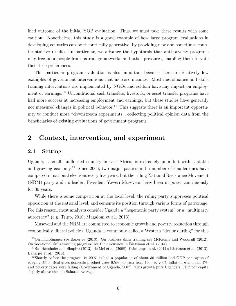
YOP was oversubscribed, and we worked with the national NUSAF office to randomizefunding among screened and eligible proposals. Thousands of groups submitted proposalsin 2006 and the NUSAF office funded hundreds in 2006-07, prior to our study. By 2008, 14NUSAF-eligible districts had funds remaining. Figure 1 maps these study districts.19
It’s important to note that the study population was only moderately affected by warand political instability. None of the most war-affected districts (Gulu, Kitgum, and Pader)had the funds to participate in the final round. Thus the districts in our study were eitheron the margins of the conflict (center north), more vulnerable to banditry and cattle raidingthan conflict (northeast) or relatively secure but underdeveloped (northwest). There arealmost no ex-combatants in the study groups. In many ways, little distinguishes our samplefrom other poor Ugandan youth.
District governments nominated 2.5 times the number of groups they could fund. Thedistricts submitted roughly 625 proposals to the national NUSAF office, who reviewed themfor completeness and validity. To minimize chances of corruption the central NUSAF of-fice also sent out audit teams to visit and verify each group. They disqualified about 70applications, mainly for incomplete information or ineligibility.20
In January 2008 the NUSAF office provided the research team with a list of 535 remaininggroups eligible for randomization, along with district budgets. We randomly assigned 265of the 535 groups (5,460 individuals) to treatment and 270 groups (5,828 individuals) tocontrol, stratified by district. Control groups were not waitlisted to receive YOP in future.During the baseline survey, before treatment status was known, groups were told they hada 50% chance of funding and that there were no plans to extend the YOP program in thefuture. Spillovers between study villages are unlikely as the 535 groups were spread across454 communities in a population of more than five million, and control groups are typicallyvery distant from treatment villages. Figure 1 also maps eligible groups per parish.
11
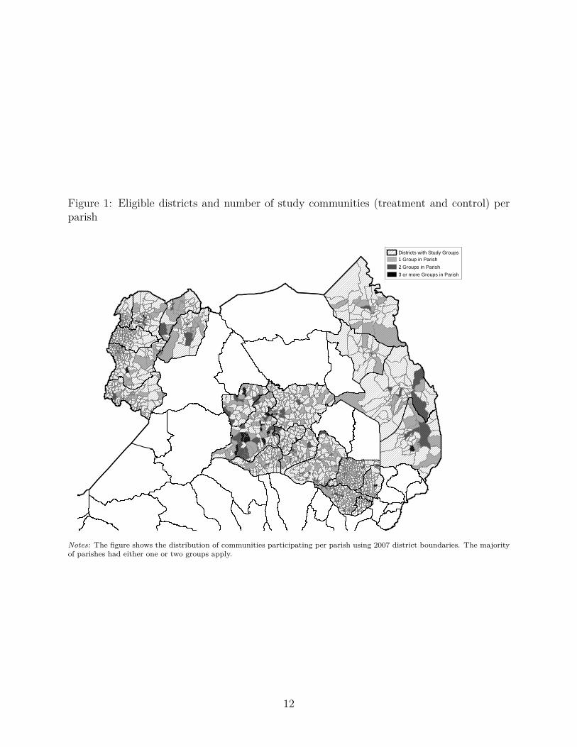
Figure 1: Eligible districts and number of study communities (treatment and control) perparish
Districts with Study Groups1 Group in Parish2 Groups in Parish3 or more Groups in Parish
Notes: The figure shows the distribution of communities participating per parish using 2007 district boundaries. The majorityof parishes had either one or two groups apply.
12
T able1:
Selected
baselin
ede
scrip
tivestatist
icsan
dtestsof
balanc
eBaseline(n=2598)
Foun
din
2010
(n=2005)
Foun
din
2012
(n=1868)
Treatm
ent–
Treatm
ent–
Treatm
ent–
Con
trol
Con
trol
Con
trol
Con
trol
Con
trol
Con
trol
Select
covariates
in2008
Mean
Diff.
p-value
Mean
Diff.
p-value
Mean
Diff.
p-value
(1)
(2)
(3)
(4)
(5)
(6)
(7)
(8)
(9)
App
lican
tgrou
psize
22.53
0.03
0.96
Grant
requ
ested,
pergrou
pmem
ber,
USD
363.05
14.09
0.25
Group
existedbe
fore
application
0.45
0.03
0.42
0.44
0.04
0.36
0.45
0.04
0.36
Individu
alun
foun
dat
baselin
e0.06
-0.05
0.00
0.25
0.01
0.47
0.30
-0.01
0.75
Age
24.75
0.17
0.55
24.94
0.20
0.48
25.06
0.06
0.84
Female
0.35
-0.02
0.38
0.36
-0.04
0.15
0.36
-0.05
0.10
Largetownor
urba
narea
0.23
-0.02
0.61
0.21
-0.02
0.65
0.18
0.01
0.84
Weeklyem
ployment,ho
urs
10.70
0.57
0.48
10.92
0.03
0.97
10.64
1.05
0.24
Allno
n-agricultural
work
5.99
-0.45
0.44
6.09
-0.73
0.25
5.82
-0.45
0.49
Allagricultural
work
4.66
1.04
0.04
4.78
0.81
0.14
4.75
1.54
0.01
Eng
aged
inaskilled
trad
e0.08
0.00
0.81
0.08
0.01
0.61
0.07
0.01
0.66
Highest
grad
ereachedat
scho
ol7.95
-0.07
0.62
7.99
-0.06
0.71
7.88
-0.09
0.60
Ableto
read
andwrite
minim
ally
0.75
-0.03
0.17
0.75
-0.03
0.14
0.74
-0.03
0.19
Receivedpriorvo
cation
altraining
0.07
0.02
0.07
0.08
0.02
0.16
0.07
0.02
0.14
Wealthindex
-0.16
0.07
0.12
-0.16
0.06
0.27
-0.17
0.05
0.40
Mon
thly
grosscash
earnings
(000s2008
UGX)
62.19
6.89
0.30
62.11
10.24
0.17
63.96
6.62
0.41
Saving
sin
past
6mo.
(00s
2008
UGX)
19.25
10.89
0.02
19.88
7.11
0.16
16.75
9.68
0.04
Can
obtain
100,000UGX
loan
0.33
0.05
0.01
0.36
0.03
0.17
0.34
0.04
0.10
Registeredto
vote
in2006
0.92
-0.01
0.57
0.93
-0.01
0.61
0.93
-0.01
0.42
Voted
in2006
presidential
election
0.73
0.03
0.21
0.73
0.04
0.08
0.75
0.00
0.91
Mem
berof
apo
litical
party
0.11
0.02
0.06
0.12
0.01
0.36
0.12
0.02
0.13
Currently
onacommun
itycommittee
0.17
0.01
0.60
0.18
0.01
0.77
0.18
0.02
0.36
Parishvote
shareforMuseveni,2006
0.32
0.00
0.99
0.32
0.00
0.82
0.31
0.00
0.95
Evermem
berof
armed
grou
p0.03
0.00
0.88
0.03
0.00
0.87
0.03
0.00
0.62
p-valuefrom
jointF-test
0.00
0.10
0.02
Not
es:Colum
ns(1),
(4),
and(7)repo
rtthemeanof
controlgrou
pmem
bers.Colum
ns(2),
(5),
and(8)repo
rtthemeandiffe
rencebe
tweenthetreatm
ent
andcontrolgrou
ps,calculated
usingan
OLS
regression
ofba
selin
echaracteristicson
anindicatorforrand
omprogram
assign
mentplus
district
fixed
effects
while
columns
(3),
(6),
and(9)repo
rtp-values.Stan
dard
errors
robu
stan
dclusteredat
thegrou
plevel.
AllUSD
andUgand
anshilling(U
GX)-deno
minated
variab
lesan
dallh
ours
workedvariab
lesweretop-censored
atthe99th
percentile
tocontainou
tliers.Baselinerefers
toallr
espo
ndents
surveyed
atba
selin
e,
while
2010
and2012
referto
therespon
dentslocatedin
each
year,r
espe
ctively.
13
2.5 Data and participants
We selected five people from each of the 535 groups to be tracked and interviewed three timesover four years—a potential panel of 2,677 people (seven were inadvertently surveyed in onegroup at baseline). We worked with Uganda’s Bureau of Statistics to conduct a baselinesurvey in February and March 2008, prior to the announcement and funding of treatmentgroups. Enumerators and local officials mobilized group members to complete a survey ofdemographic data on all members as well as group characteristics. Virtually all memberswere mobilized, and we randomly selected five of the members present to be individuallysurveyed and tracked.21 The NUSAF office disbursed funds between July and September2008 via the central bank.
Working with private, independent survey organizations, we conducted the first 2-yearendline survey between August 2010 and March 2011, 24 to 30 months after disbursement.We conducted a 4-year survey between April and June 2012, 44 to 47 months after disburse-ment, and just over a year after the 2011 national elections.
Participants
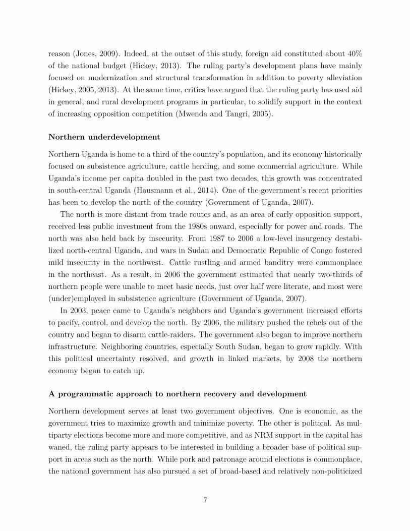
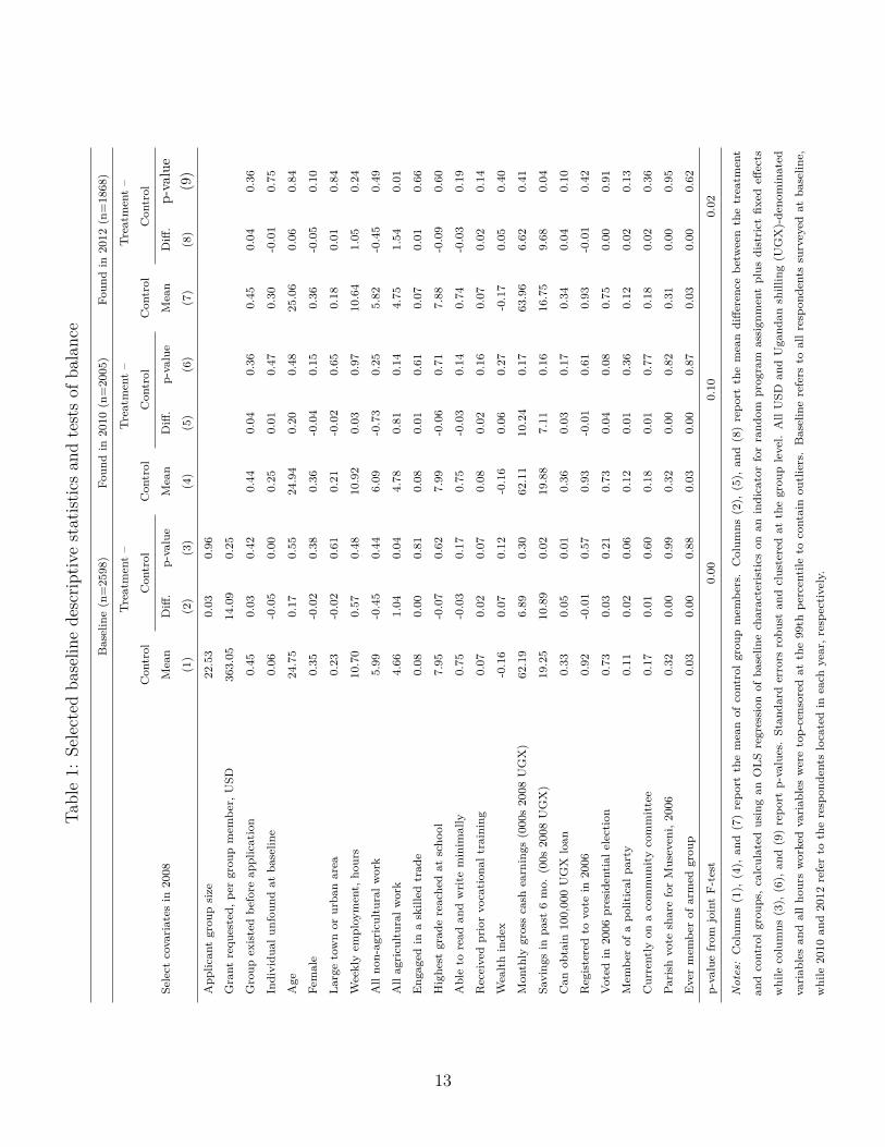
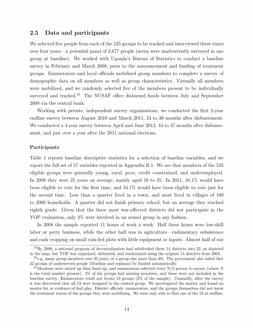
Table 1 reports baseline descriptive statistics for a selection of baseline variables, and wereport the full set of 57 variables reported in Appendix B.1. We see that members of the 535eligible groups were generally young, rural, poor, credit constrained, and underemployed.In 2008 they were 25 years on average, mainly aged 16 to 35. In 2011, 16.1% would havebeen eligible to vote for the first time, and 34.1% would have been eligible to vote just forthe second time. Less than a quarter lived in a town, and most lived in villages of 100to 2000 households. A quarter did not finish primary school, but on average they reachedeighth grade. Given that the three most war-affected districts did not participate in theYOP evaluation, only 3% were involved in an armed group in any fashion.
In 2008 the sample reported 11 hours of work a week. Half these hours were low-skilllabor or petty business, while the other half was in agriculture—rudimentary subsistenceand cash cropping on small rain-fed plots with little equipment or inputs. Almost half of our
19By 2008, a national program of decentralization had subdivided these 14 districts into 22, as depictedin the map, but YOP was organized, disbursed, and randomized using the original 14 districts from 2003.
20e.g. many group members over 35 years, or a group size more than 40). The government also asked that22 groups of underserved people (Muslims and orphans) be funded automatically.
21Members were mixed up then lined up, and enumerators selected every N/5 person to survey (where Nis the total number present). 4% of the groups had missing members, and these were not included in thebaseline survey. Enumerators could not locate 13 groups (3% of the sample). Unusually, after the surveyit was discovered that all 13 were assigned to the control group. We investigated the matter and found nomotive for or evidence of foul play. District officials, enumerators, and the groups themselves did not knowthe treatment status of the groups they were mobilizing. We were only able to find one of the 13 at endline.
14
sample reported no employment in the past month, and only 8% were engaged in a skilledtrade. Cash earnings in the past month averaged a dollar a day. Savings in the past sixmonths were $15 on average, and only 11% reported any savings.22
Although poor by any measure, these applicants were slightly wealthier and more ed-ucated than their peers. If we compare our sample to their age group and gender a 2008population-based household survey, our sample has 1.7 years more education, 0.15 standarddeviations more wealth, is 7.5 percentage points more urban and 5.4 percentage points morelikely to be married, and has 1.6 fewer household members (see Appendix A.2).
Tracking and panel attrition
YOP applicants were a young, mobile population. Nearly 40% had moved or were awaytemporarily at each endline survey. To minimize attrition we used a two-phase trackingapproach, as outlined in Appendix A.3. In the first phase we tracked all 2,677 membersof the sample, and in a second phase we did intensive tracking of a randomized sampleof unfound people. Our response rate was 97% at baseline, and effective response rates atendline (weighted for selection into endline tracking) were 85% after two years and 82% afterfour.
Of slightly greater concern is correlation between attrition and treatment, reported inAppendix Table A.3. The treatment group was 5 percentage points more likely to be foundat baseline in 2008. There is no treatment-control imbalance in 2010, although controls aremore likely to have been lost in 2008 and the treatment group in 2010. In 2012, controls were7 percentage points less likely to be found. If unfound controls are particularly successful, wecould overstate the impact of the intervention. Such bias is conceivable: baseline covariatesare significantly correlated with attrition and the unfound tend to be younger, poorer, lessliterate farmers from larger communities (see Appendix B.2). For this reason our treatmenteffects estimates will control for baseline characteristics associated with attrition, and wewill test the sensitivity of results to various attrition scenarios.
2.6 Randomization balance
The computer-based randomization generated some imbalances across treatment arms. Wereport balance tests for selected variables in Table 1 (for the full list see Appendix B.1).For instance, at baseline the treatment group report 2 percentage points more vocationaltraining, 0.07 standard deviations greater wealth, 56% greater savings (though only in the
2233% held loans, but these were small: under $7 at the median among those who have any loans, mainlyfrom friends and family. About 10% reported they could obtain a large loan of 1,000,000 UGX (about $580).
15
linear, not in log form), and 5 percentage points more access to small loans. Of 57 covariates,6 (10.5%) of the treatment-control differences have p < 0.05, and 8 (14.0%) have p < 0.10. Atest of joint significance from an OLS regression on treatment assignment treatment indicatorreveals that baseline characteristics are jointly significant with p = 0.05.
The missing 13 control groups could cause the imbalance. We estimate that if the miss-ing controls had baseline values 0.1 to 0.2 standard deviations above the control mean, itwould account for the full imbalance (see Appendix B.3). If so, the observed control groupmay be poorer than the treatment group, and will overstate true program impacts. Ourempirical strategy and sensitivity analysis below explicitly address the concerns that arisefrom imbalance and potentially selective attrition.
2.7 Empirical strategy
In designing the experiment, our primary outcomes of interest were the direct economic ef-fects of the business planning and cash on economic performance: investments in trainingand business assets, levels and type of employment, and incomes.23 The longer-term polit-ical impacts were of interest from the beginning, but we did not identify them as primaryoutcomes, in part because any political effects were likely to be indirect and a function of suc-cessful economic impacts. Thus, as with any set of downstream impacts (and like most otherevaluations of the political effects of public programs), the treatment effects on secondaryoutcomes should be treated with some caution.
We estimate intent-to-treat (ITT) effect on outcomes, Y , via the weighted least squares(WLS) regression:
Yij = θIT TT ij + βXij + γd + εij
where T is an indicator for assignment to treatment for person i in group j, X is the vector ofbaseline covariates displayed in Appendix Table B.1, the γ are district fixed effects (requiredbecause the probability of assignment to treatment varies by strata), and ε is an error termclustered by group. We weight observations by their inverse probability of selection intoendline tracking.
23The 4-year outcomes were derived from a formal model and pre-specified in the analysis of the 2-yearresults. As the experiment pre-dated the social science registry, the trial was not formally pre-registered.
16

Table 2: Economic impacts of the program after four years2010 (N=2,005) 2012 (N=1,868)
Control ITT, with controls Control ITT, with controls
Dependent variable in 2012 Mean Mean SE Mean Mean SE
(1) (2) (3) (4) (5) (6)
Transfers and investment
Group received YOP cash transfer 0.000 0.886 [0.019]***
Business assets (000s 2008 UGX) 290.2 377.0 [78.217]*** 392.8 225.0 [62.601]***
Employment
Average employment hours per week 24.9 4.1 [1.070]*** 32.2 5.5 [1.284]***
No employment hours in past month 0.100 -0.011 [0.015] 0.05 -0.022 [0.009]***
Engaged in any skilled trade 0.170 0.272 [0.025]*** 0.22 0.261 [0.026]***
Income
Index of income measures, z-score -0.05 0.17 [0.049]*** -0.06 0.24 [.049]***
Monthly cash earnings (000s 2008 UGX) 35.2 14.61 [4.073]*** 47.8 18.19 [4.898]***
Durable assets (z-score) -0.06 0.101 [0.047]** 0.150 0.181 [0.055]***
Non-durable consumption (z-score) -0.011 0.180 [0.051]***
Notes: Columns (1) and (4) report the control group mean, weighted by the inverse probability of selection into
each endline sample. Columns (2)-(3) and (5)-(6) report the intent-to-treat (ITT) estimate and standard error
(SE) of program assignment at each endline. Standard errors are heteroskedastic-robust and clustered by group.
We calculate the ITT via a weighted least squares regression of the dependent variable on a program assignment
indicator, 13 district (randomization stratum) fixed effects, and a vector of control variables that includes all of the
baseline covariates reported in Appendix B.1. Continuous economic outcomes such as hours worked and earnings
have a long upper tail, and some of these large values are potentially due to enumeration errors. Extreme values
will be highly influential in any treatment effect, so we top-code all currency-denominated, hours worked, and
employee variables at the 99th percentile.
3 Economic impacts of the program
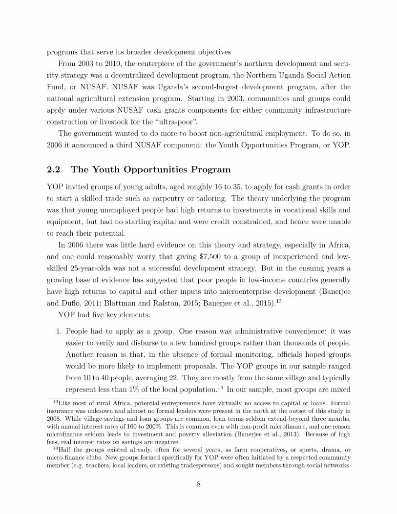
YOP led to large and persistent increases in investment, work, and income. Table 2 reportsITT estimates on economic outcomes two and four years after the interventions, as doc-umented in our companion paper economic impacts of YOP (Blattman et al., 2014). Wesummarize them here before moving on to the political impacts.
Compliance Of the 265 groups assigned to a cash grant, 89% received it. 21 groups couldnot access funds because of problems with identifying the group leaders and banking details,bank complications, collection delays, or corruption.24
24Only 8 groups reported that they never received funds due to some form of theft or diversion. The groupswho did and did not receive funds (for any reason) are generally similar along baseline characteristics, butgroups were slightly more likely to be treated if they were educated and wealthier and did not have too manymembers (regressions not shown). These traits probably lowered the probability of a disqualifying error inthe proposals.
17
Investments A majority of groups and members invested the funds in skills training andbusiness materials, as planned. Between 2008 and 2010, 68% of the treatment group enrolledin vocational training, compared to 15% of the control group and, on average, treatmenttranslated into 340 more hours of vocational training than controls. Among those whoenrolled in any training, 38% trained in tailoring, 23% in carpentry, 13% in metalwork, 8%in hairstyling, and the remainder in miscellaneous other trades.
Even so, the majority of the grants were invested in capital, as the median group estimatedthey spent just 11% on skills training, compared to 65% on tools and materials (the remaining24% was shared in cash or spent on other things).25 The control group reported UGX 290,200($167) of business assets in 2010 and UGX 392,800 ($228) in 2012. By 2010 treatment hadincreased capital stocks by UGX 377,023 ($219), a 131% increase over the control group. By2012 stocks had increased by UGX 224,986 ($130), a 57% increase over the control group.
Afterwards, group members typically went their own way to start individual businessesrather than form firms or cooperatives.26
Employment impacts With these investments, YOP led these young people to shift theiroccupations toward skilled work and cottage industry, thus increasing their labor supplyoverall. After four years, people in groups assigned to receive a grant were more thantwice as likely to practice a skilled trade—typically as self-employed artisan in carpentry,metalworking, tailoring, or hairstyling. After four years the treatment group worked 5.5more hours weekly than the control group—a 17% increase.
Income impacts YOP’s ultimate aim was to reduce poverty, and these capital investmentsand increases in labor supplied were means to an end: increases in earned income. Incomeis notoriously difficult to measure, especially in poor and rural areas (like northern Uganda)where the average person has volatile and seasonal work, multiple sources of income, andboth monetary and in-kind remuneration. We measured income in three ways: self-reportedearnings, consumption assets owned, and an estimate of total household consumption. The
25Our survey data and qualitative interviews suggest that groups made bulk purchases of tools and othermaterials, but these were distributed and individually owned. Groups commonly elected management com-mittee members to handle procurement, making major training and tool purchases in bulk, largely for thecost savings involved. These tools were typically distributed equally to individual members, but about halfthe respondents said they shared some small or large tools with other group members. In the 2010 survey,90% of group members said they felt the grant was equally shared, and 92% said the leaders received nomore than their fair share. Most of the remainder reported only minor imbalances.
26Nearly all treatment groups reported meeting together after the grant, typically several times a year.Half said their facilitator still engaged with the group, in part because they are from the area, had previousties to the group, or were interested in their progress. Control groups reported meeting just as frequently, inlarge part because many of these groups preexisted and serve other purposes, and part because they hopedto receive transfers in the future.
18
consumption and asset measures are thought to be better measures of stable or “permanent”income.27
All three measures increase significantly in the treatment group, as does a mean effectsindex of all three measures standardized to have mean zero and unit standard deviation.This overall index is useful for summarizing the three measures and reducing the numberof hypotheses we test. It suggests that YOP increased incomes by 0.17 standard deviationsafter two years and by 0.24 standard deviations after four years. But while this index reducesmultiple comparison concerns, the components give a more concrete sense of the impacts.
The control group reported monthly cash earnings of UGX 30,825 ($18) in 2008, UGX35,200 ($20) in 2010, and UGX 47,800 ($28) in 2012.28 Such growth may have come in partfrom a growing economy, but it also arose from young people gradually increasing their hoursworked, capital stocks, and output over time by investing earnings. Assignment to receivea YOP grant increased monthly earnings by UGX 14,605 ($8.50) in 2010 and UGX 18,186($10.57) in 2012. This earnings increase is modest in absolute terms—just under a dollar aday in PPP terms. But relative to the control group’s earnings this is a roughly 40% increasein earnings—a hugely important change for someone earning so little per day. We see similarpatterns in two alternative measures of income: durable and nondurable consumption. Bothrose over time and had large program effects.
Both men and women benefited from the program. A third of applicants were womenand the program had large and sustained impacts on them: After four years, incomes oftreatment women were 73% greater than control women, compared to a 29% gain for men.Over the four years, control men kept pace or caught up with treatment men. Womenstagnated without the program but took off when funded.
These are extremely large impacts, especially considering how few employment programseven pass a simple cost-benefit test. Blattman and Ralston (2015), in their review of theevidence of the effectiveness of employment programs in poor, middle-income, and high-income countries, identify the YOP program (and cash transfer programs like it) as some ofthe highest return employment programs with evidence in the world.
27See Blattman et al. (2014) for a full discussion.28The 2008 survey has data on gross cash revenues only, whereas gross and net earnings are available in
2010. For the 2008 value of net earnings, we use the 2008 gross amount multiplied by the 2010 ratio of grossto net. This number is merely for descriptive purposes and has no bearing on treatment effect estimates.
19
4 Impacts of the program on political behavior
4.1 Theoretical motivation
YOP is unlike the sort of clientelistic program most commonly used in transactional politicsand vote-buying, such as public sector jobs: it was a large-scale state employment programthat was foreign-financed, relatively technocratic and non-politicized in its targeting andimplementation, and (unlike a public sector job) the grant was by its nature impossible torevoke once given.29 Indeed, it transferred resources directly to voters, much like land titling,conditional cash transfers, or skills training or other public programs. These are commonlylabeled “programmatic policies” rather than pork programs or traditional patronage.
There is a growing base of evidence that voters reward incumbents for programmaticpolicy, at least in aggregate. For instance, comparing areas with varying exposure to con-ditional cash transfer programs in Latin America, Manacorda et al. (2011); Zucco (2013);Diaz-Cayeros et al. (2016) argue that retrospective voting could account for the fact thatareas that received more assistance rewarded incumbents, sometimes even after the programbenefits had finished.30 Similarly, Casaburi and Troiano (2015) see an increase in incum-bent vote share after a successful anti-tax evasion program, and Larreguy et al. (2015) seeincumbent vote share rise after a land titling program.
The literature provides several plausible reasons why people assigned to treatment shouldreward the ruling party at the polls for programmatic policies, and together they led us tohypothesize that assignment to treatment would increase partisanship and electoral supportfor the NRM and Museveni.
The first reason, commonly called “pocketbook voting”, argues that economically suc-cessful voters tend to reward the incumbent (Kramer, 1971; Fiorina, 1976). Overall, YOPrecipients experienced a large increase in wealth and may have rewarded the incumbent asa consequence, independently of whom they attribute the responsibility of the program to.This idea that voters are naïve and make simple calculations is supported by the literatureon how natural events, shark attacks or football games, can sometimes boost incumbents’popularity (Healy et al., 2010; Achen and Bartels, 2004). One explanation is that poorly
29One important different between conditional and unconditional transfers is the amount of interactionindividuals have with government. In the YOP case, young people interacted with the government, but in alimited way and only during the application process or, in limited cases, briefly after receiving funds. Mostconditional cash programs deliver money in tranches over long periods of time, requiring greater interactionswith officials and more reliance on the continuation of the distribution. YOP participants neither needednor expected further interactions with government after receiving the program.
30In one case, that of conditional cash transfers in Mexico, it is contested whether incumbent vote shareincreased, or whether the effect was purely on turnout (Schober, 2016). Nonetheless, the argument thatincumbent vote share responds to programmatic policy extends well beyond Mexico.
20
informed voters interpret good fortune as plausible new information about an incumbent’squality or characteristics (Ashworth et al., 2016).
A second reason is the theory of retrospective voting, where voters reward incumbentsbecause they interpret development programs as a signal that the incumbent is effective,or that the incumbent will work to benefit voters like themselves in the future. Relatedly,some theories emphasize reciprocity in voting—that voters reward incumbents out of a senseof gratitude or perceived obligation—and this would generate similar predictions to retro-spective voting: increased vote share for the incumbent, at least when they attribute theprogram to that party or politician.
The YOP program was one of the largest development program ever run in Uganda.As such YOP could be viewed as a costly signal from the ruling party that it intended tochannel more funds in the future to the north of the country, thus changing the expectedbenefits of keeping the party in power.31 This led us to predict that YOP beneficiaries mightreciprocate with votes for the ruling party.
In general, at the outset of the study there was little theoretical apparatus or litera-ture leading us us to predict the opposite effect: that YOP could augment support for theopposition. We return to this question in the discussion and conclusions section below.
4.2 National election outcomes
YOP was first and foremost an employment program, and so the economic outcomes reportedabove were our primary and pre-specified outcomes. Nonetheless, the literature on the effectsof central government programs on national political support led us to add questions onpartisanship and electoral behavior (before and after the election) to the endline survey. Wefocus on these outcomes here, starting with partisan attitudes and actions.
Partisan attitudes and actions
Three years after the grants, we see no evidence that the program increased general politicalparticipation or support for the ruling party. Rather, if anything, young people assigned tothe treatment increased their support for the opposition.
31Of course, for there to be a differential effect on treated individuals, the actual receipt of YOP wouldhave to change these expectations. It is possible that treatment and control group members would see orabsorb the signal differently. For instance, NUSAF was widely perceived as corrupt. But those who actuallyreceived the grants have direct evidence that it reaches people like them. Also, any element of reciprocitywould likely affect the actions of YOP recipients. That said, were non-recipients to reward the incumbentfor good policy, this would attenuate the treatment effects in our experiment. This highlights one of thekey differences that separates our study from previous ones: we examine variation between treated andnon-treated individuals in the same locality, rather than treated and non-treated localities.
21

Table 3: Program impacts on partisan attitudes and actions, by incumbent and oppositionparty
2012 sample
(1) (2) (3) (4)
Control ITT, with controls
Dependent variable in 2012 Mean Coeff. Std. Err. N
Index of NRM/Presidential support (z-score) -0.05 -0.04 [.052] 1,858
Would vote NRM if election tomorrow 0.75 -0.02 [.022] 1,858
Like or strongly like the NRM 0.81 -0.02 [.02] 1,845
Feels close to the NRM 0.55 0.01 [.024] 1,833
Worked to get the NRM elected 0.29 0.01 [.023] 1,844
Member of the NRM 0.40 -0.02 [.026] 1,849
Voted or supported the President in 2011 0.88 -0.04 [.018]** 1,755
Approve or strongly approve of President 0.85 -0.02 [.018] 1,847
Index of opposition support (z-score) 0.00 0.11 [.053]** 1858
Would vote opposition if election tomorrow 0.17 0.01 [.020] 1858
Like or strongly like any opposition party 0.36 0.03 [.023] 1844
Feels close to any opposition party 0.10 0.03 [.016]** 1833
Worked to get the opposition elected 0.04 0.03 [.011]*** 1844
Member of an opposition party 0.05 0.02 [.013]** 1849
Voted or supported an opposition party in 2011 0.12 0.04 [.018]** 1755
Notes: Column (1) reports the control group mean, weighted by the inverse probability of se-
lection into each endline sample. Columns (2)-(3) report the estimated intent-to-treat (ITT)
coefficient and standard error at endline. Standard errors are heteroskedastic-robust and clus-
tered by group. The number of observations in Column 4 may differ from the total number of
people survey (1,868) because a small number of people, typically less than 1–2%, declined to
answer the political questions.We calculate the ITT via a weighted least squares regression of
the dependent variable on a program assignment indicator, 13 district (randomization stratum)
fixed effects, and a vector of control variables that includes all of the baseline covariates reported
in Appendix B.1.
22
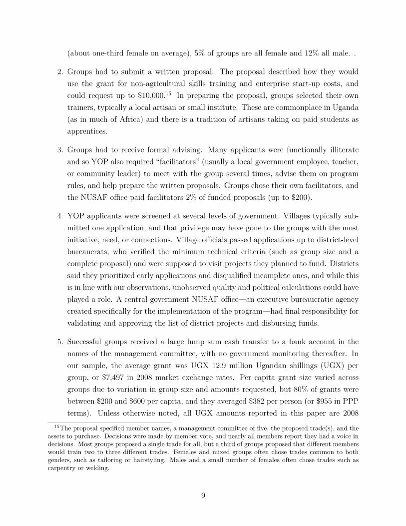
Table 3 reports our main results on the impacts of receiving the program on politicalbehavior and attitudes towards the ruling party and opposition parties. To reduce thenumber of hypotheses being tested, we group outcomes thematically into a small number offamilies and calculate a standardized mean effects index of all component outcomes.32 Notethat the survey was conducted four years after the grant and a year after the last election.Party and political attitudes (e.g. support for the ruling party) are reported at the timeof the survey, while electoral participation and political actions (e.g. attending a rally) areretrospective measures of pre-election and election activities. For causal identification, thisrequires that recall error is not correlated with treatment status.
First, an index of ruling party support—vote intentions, support for, work for, and mem-bership in the ruling party, plus support for the President in particular—falls by 0.05 stan-dard deviations. This is not statistically significant but the sign of the coefficient is theopposite of what we expected. Moreover, while 88% of the control group voted for the Pres-ident, this declined by 4 percentage points with treatment, significant at the 5% level. Thislatter result would not hold after correcting for multiple hypotheses within the family, andso we must take it cautiously, but it is worth noting that it is probably the most importantpolitical indicator for the national government and it runs in the opposite direction of ourprediction.33 We can certainly rule out an increase in support for the ruling party.34
Second, support for and actions on behalf of an opposition party increased by 0.11 stan-dard deviations among those assigned to treatment. The vast majority of opposition supportis for Kizza Besigye and his party, the FDC, but we pool all opposition candidates for thisanalysis. Looking at the components of this family index, all treatment effects are positive.35
The proportionally largest and statistically significant changes are to feeling close to the op-position party, working for the opposition, being a member of the opposition and actualvoting for the opposition. In this context, “working to get a candidate elected” can include
32We standardize the components, average them, and re-standardize. Thus each component receives equalweight.
33If we adjust for seven comparisons within the family, the coefficient on voting for the President has ap-value of 0.24. We use the Westfall and Young (1993) free step-down resampling method for the family-wiseerror rate (FWER), the probability that at least one of the true null hypotheses will be falsely rejected, usingrandomization inference.
34Parish-level data also supports the view that the program’s effect on support for the ruling party waslimited. Using parish-level voting returns in 2011, we can examine the impact of having at least one NUSAFgroup assigned in the parish, to see if local populations reward the President for targeting the parish with anyNUSAF project, including a YOP project. Support for the President is 2.2 percentage points higher in thesedistricts, with a standard deviation of 0.015 (not statistically significant.Table not shown, but the regressionis analogous to the treatment effects estimated above. There are 420 eligible parishes in the sample.
35One feature of our population is that they are mainly under 35, with about a quarter eligible to vote forthe first time. As we illustrate in Appendix B.5, the results are not driven by these young and inexperiencedvoters. There is no statistically significant difference between first time and older voters, and if anything theaverage treatment effect is slightly higher when we exclude first time voters.
23
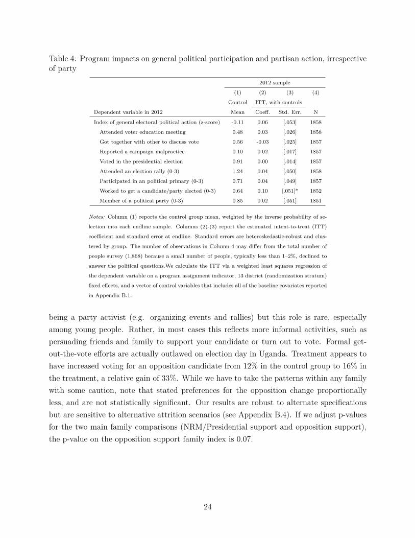
Table 4: Program impacts on general political participation and partisan action, irrespectiveof party
2012 sample
(1) (2) (3) (4)
Control ITT, with controls
Dependent variable in 2012 Mean Coeff. Std. Err. N
Index of general electoral political action (z-score) -0.11 0.06 [.053] 1858
Attended voter education meeting 0.48 0.03 [.026] 1858
Got together with other to discuss vote 0.56 -0.03 [.025] 1857
Reported a campaign malpractice 0.10 0.02 [.017] 1857
Voted in the presidential election 0.91 0.00 [.014] 1857
Attended an election rally (0-3) 1.24 0.04 [.050] 1858
Participated in an political primary (0-3) 0.71 0.04 [.049] 1857
Worked to get a candidate/party elected (0-3) 0.64 0.10 [.051]* 1852
Member of a political party (0-3) 0.85 0.02 [.051] 1851
Notes: Column (1) reports the control group mean, weighted by the inverse probability of se-
lection into each endline sample. Columns (2)-(3) report the estimated intent-to-treat (ITT)
coefficient and standard error at endline. Standard errors are heteroskedastic-robust and clus-
tered by group. The number of observations in Column 4 may differ from the total number of
people survey (1,868) because a small number of people, typically less than 1–2%, declined to
answer the political questions.We calculate the ITT via a weighted least squares regression of
the dependent variable on a program assignment indicator, 13 district (randomization stratum)
fixed effects, and a vector of control variables that includes all of the baseline covariates reported
in Appendix B.1.
being a party activist (e.g. organizing events and rallies) but this role is rare, especiallyamong young people. Rather, in most cases this reflects more informal activities, such aspersuading friends and family to support your candidate or turn out to vote. Formal get-out-the-vote efforts are actually outlawed on election day in Uganda. Treatment appears tohave increased voting for an opposition candidate from 12% in the control group to 16% inthe treatment, a relative gain of 33%. While we have to take the patterns within any familywith some caution, note that stated preferences for the opposition change proportionallyless, and are not statistically significant. Our results are robust to alternate specificationsbut are sensitive to alternative attrition scenarios (see Appendix B.4). If we adjust p-valuesfor the two main family comparisons (NRM/Presidential support and opposition support),the p-value on the opposition support family index is 0.07.
24

General political behavior
Increased political action seems to be concentrated among opposition supporters, since itis not associated with a similar increase in political participation in the full sample. Table4 reports impacts on political participation in general, irrespective of party. These includemeasures from Table 3 where we ignore the ruling party/opposition distinction, but alsoincludes non-partisan political participation (or potentially partisan measures where we donot know the party in question, such as attending a rally).
The program had little effect on the general index of political participation or any ofthe individual components: whether someone attended voter education meetings, met withothers to discuss the election, reporting of malpractice or even whether they voted in thepresidential election. The family index rises by 0.06 standard deviations but has a p-valueof 0.262. 91% of the sample reported voting, perhaps leaving little room for improvementon this metric, but we likewise see no improvement in the other measures of participation.
The program also had no statistically significant effect on general partisan actions—including attending a political rally, participating in a primary, working to get a candidateelected, or being a member of a party. Only one component measure shows any evidenceof change: self-reporting working to get a party elected increased from 64% in the controlgroup to 74% in the treatment, significant at the 10% level. These effects are largely drivenby the increase in activity on behalf of the opposition.
4.3 Subnational election outcomes
As we will see below, more than 87% of respondents attributed the YOP program to thenational government and ruling party. Nonetheless, given the close involvement of subcountyand district officials in the nomination process, we anticipated that beneficiaries might rewardlocal candidates as well. These could include local councilors at the district level (calledLC5s), at the subcounty level (called LC3s) and the village level (called LC1s).
Table 5 displays the program’s impact on support for incumbent LC5s who served duringthe YOP disbursement and re-ran for election (about half of all races). It also displaystreatment effects for whether the individual voted in the LC5 election (a measure of localpolitical participation), and also the approval for current local councilors. We are principallyinterested in support for incumbent LC5s, and we break down support based on whether theLC5 was NRM or opposition.
Treatment led to a 0.057 percentage point decrease in voting for or supporting the in-cumbent LC5, regardless of party (not statistically significant). However, looking at thesubgroups reveals that support for NRM incumbents fell dramatically, by 12.5 percentage
25
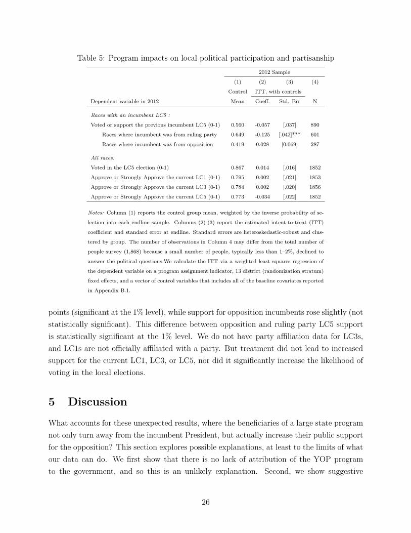
Table 5: Program impacts on local political participation and partisanship2012 Sample
(1) (2) (3) (4)
Control ITT, with controls
Dependent variable in 2012 Mean Coeff. Std. Err N
Races with an incumbent LC5 :
Voted or support the previous incumbent LC5 (0-1) 0.560 -0.057 [.037] 890
Races where incumbent was from ruling party 0.649 -0.125 [.042]*** 601
Races where incumbent was from opposition 0.419 0.028 [0.069] 287
All races:
Voted in the LC5 election (0-1) 0.867 0.014 [.016] 1852
Approve or Strongly Approve the current LC1 (0-1) 0.795 0.002 [.021] 1853
Approve or Strongly Approve the current LC3 (0-1) 0.784 0.002 [.020] 1856
Approve or Strongly Approve the current LC5 (0-1) 0.773 -0.034 [.022] 1852
Notes: Column (1) reports the control group mean, weighted by the inverse probability of se-
lection into each endline sample. Columns (2)-(3) report the estimated intent-to-treat (ITT)
coefficient and standard error at endline. Standard errors are heteroskedastic-robust and clus-
tered by group. The number of observations in Column 4 may differ from the total number of
people survey (1,868) because a small number of people, typically less than 1–2%, declined to
answer the political questions.We calculate the ITT via a weighted least squares regression of
the dependent variable on a program assignment indicator, 13 district (randomization stratum)
fixed effects, and a vector of control variables that includes all of the baseline covariates reported
in Appendix B.1.
points (significant at the 1% level), while support for opposition incumbents rose slightly (notstatistically significant). This difference between opposition and ruling party LC5 supportis statistically significant at the 1% level. We do not have party affiliation data for LC3s,and LC1s are not officially affiliated with a party. But treatment did not lead to increasedsupport for the current LC1, LC3, or LC5, nor did it significantly increase the likelihood ofvoting in the local elections.
5 Discussion
What accounts for these unexpected results, where the beneficiaries of a large state programnot only turn away from the incumbent President, but actually increase their public supportfor the opposition? This section explores possible explanations, at least to the limits of whatour data can do. We first show that there is no lack of attribution of the YOP programto the government, and so this is an unlikely explanation. Second, we show suggestive
26
evidence that increase in wealth is a major driver of this change in behavior, consistentwith a mechanism already suggested in the literature: wealthier people feel freer to votetheir conscience, possibly because they are less tied to patronage networks or less reliant onlocal politicians and strongmen. Indeed, YOP beneficiaries were less likely to be mobilizedon election day. That said, they are not less likely to be enmeshed in general patronagerelations, perhaps because their greater wealth brings some influence.
Before developing these more substantive explanations, however, we should note thatall of our data are self-reported and vulnerable to systematic measurement error. Nonethe-less, we think it’s unlikely that measurement error accounts for our results. If those whoreceived YOP were more likely to report voting for the opposition, or otherwise expressingtheir opposition preferences publicly, then this could account for the treatment effects weobserve. This could arise because the control group aspires to future government programsand thinks that saying they voted for the President will increase their chances, even whentalking to a supposedly independent study firm. We cannot eliminate this possibility. Suchmeasurement error, however, is difficult to reconcile with the pattern of treatment effects weobserve, in particular the absence of any impact on attitudes towards the ruling party andits challengers. It is possible that treatment affects the likelihood of reporting oppositionvoting/membership/activities but not party support, but this narrows the set of plausiblesystematic measurement error stories that could explain our results.
5.1 Did the ruling party get credit for NUSAF? Program attri-bution and beliefs
One possibility is that respondents did not attribute the YOP program, or their own selectioninto the program, to the ruling party. We see little evidence for this view. While a majorityof our sample of YOP applicants attributed the program to the national government, theydid not perceive YOP as a political favor, a form of patronage, or even a gift. Ratherrespondents viewed YOP as programmatic in nature. While this programmatic perceptionmight explain the absence of any increase in ruling party support, it is hard to see howit explains the decline in Presidential voting or increased electoral action on behalf of theopposition.
Table 6 presents summary statistics and treatment effects on respondents’ beliefs aboutthe program. NUSAF was widely perceived as programmatic, in that 92% of the controlgroup said the purpose of NUSAF was northern development, versus 6% who said it was toincrease political support.
Most respondents attributed the broader NUSAF program (including YOP) to either the
27

Table 6: Self-reported beliefs about the NUSAF programControl
(n=932)
Treatment
(n=924)
Regression
Difference
Dependent variable in 2012 Coeff. p-value
(1) (2) (3) (4)
Who was mainly responsible for giving N. Uganda the NUSAF program?
The President/NRM/national government 0.555 0.523 -0.034 0.131
District or local politician/official 0.013 0.012 0.001 0.755
Foreign donor (e.g. World Bank, NGO) 0.319 0.364 0.041 0.056
Don’t Know 0.125 0.110 -0.010 0.529
What do you think the main motivation was in giving YOP to the people of northern Uganda?
To develop/assist the north 0.916 0.910 0.006 0.601
To increase political support 0.055 0.064 -0.001 0.926
To make donors happy 0.009 0.002 -0.008 0.026
Don’t know 0.020 0.024 0.003 0.697
Who selected groups to receive YOP funding?
National government 0.071 0.080 0.003 0.826
District chairperson (elected official) 0.063 0.092 0.009 0.461
NUSAF district technical officer 0.340 0.403 0.074 0.001
District executive committee 0.077 0.096 0.016 0.212
Community facilitator 0.100 0.077 -0.019 0.143
No answer 0.348 0.251 -0.081 0.000
Why were groups chosen/not chosen for funding?
The best quality projects were selected 0.131 0.449 0.317 0.000
Hard work of group leaders/facilitators 0.152 0.233 0.090 0.000
Bribe to facilitator 0.009 0.010 0.002 0.692
Relationship with district chairperson 0.071 0.019 -0.043 0.000
Random 0.157 0.095 -0.063 0.000
Don’t know 0.479 0.194 -0.303 0.000
Do you think the selection was fair? 0.424 0.828 0.402 0.000
Thinks likely to receive future program next year 0.753 0.759 0.037 0.070
Notes: Columns (1) and (2) report the control and treatment group means, weighted by the
inverse probability of selection into each endline sample. Columns (3)-(4) report the intent-to-
treat (ITT) estimated coefficient and p-value from YOP program assignment. Standard errors are
heteroskedastic-robust and clustered by group. We calculate the ITT via a weighted least squares
regression of the dependent variable on a program assignment indicator, 13 district (randomization
stratum) fixed effects, and a vector of control variables that includes all of the baseline covariates
reported in Appendix B.1.
28
central government (56% of the control group) or a foreign donor (32%), typically the WorldBank. Both answers were correct, since NUSAF was funded via a large credit from the WorldBank, and the government received significant technical assistance from the World Bank toimplement.36 People assigned to treatment were slightly more likely to assign the programto a foreign donor, but the difference is not large.
However, when asked who was the main group or individual responsible for selecting thegroups for funding, only 15.7% recalled that the selection was random. Instead, the majorityof respondents either did not know or identified their district NUSAF technical official (anunelected bureaucratic position) as responsible for funding. Those assigned to treatmentwere more likely to assign responsibility to the local NUSAF technical officer, perhaps dueto the fact that this officer was in frequent contact with treatment groups throughout theprogram.
The fact that groups did not identify the national government as responsible for fundingselection could explain why treated individuals were less likely to reward the government.But we see only modest evidence that treatment effects on partisanship varied with programattribution. Table 7 reports an ITT regression where we include post-treatment governmentattribution as a covariate, and interact it with treatment. Unfortunately, we do not havepre-treatment data on attribution, which means we have to interpret results with caution.Nonetheless, the coefficients on treatment and the treatment interaction in Table 7 suggestthat the increase in opposition support is not limited to the people who attribute the pro-gram to a foreign donor. On average, those who attribute YOP to someone other than thegovernment increase their support for the opposition by 0.168 standard deviations. Oppo-sition support is 0.090 standard deviations lower among those who attribute YOP to thegovernment, but the coefficient on the interaction is not statistically significant. (It is alsoworth noting that this difference is overstated to the extent that people who came to supportthe opposition post-program are less likely to be charitable towards the government and givethem responsibility for YOP.)
We also see little effect of beliefs about program selection on the opposition supporttreatment effects. Among those who thought program selection was fair, opposition supportrose by 0.13 standard deviations, compared to 0.121 standard deviations among those whoperceived selection as unfair. Among those who thought program selection was random,opposition support rose 0.169 standard deviations, compared to 0.123 standard deviationsamong those who perceived selection as non-random (see Appendix B.6).
Overall, a lack of attribution could help explain why the ruling party did not get rewarded36Regrettably, multiple answers were not collected on this survey question, and so we cannot be sure that
people did not attribute the program both to the government and the World Bank.
29
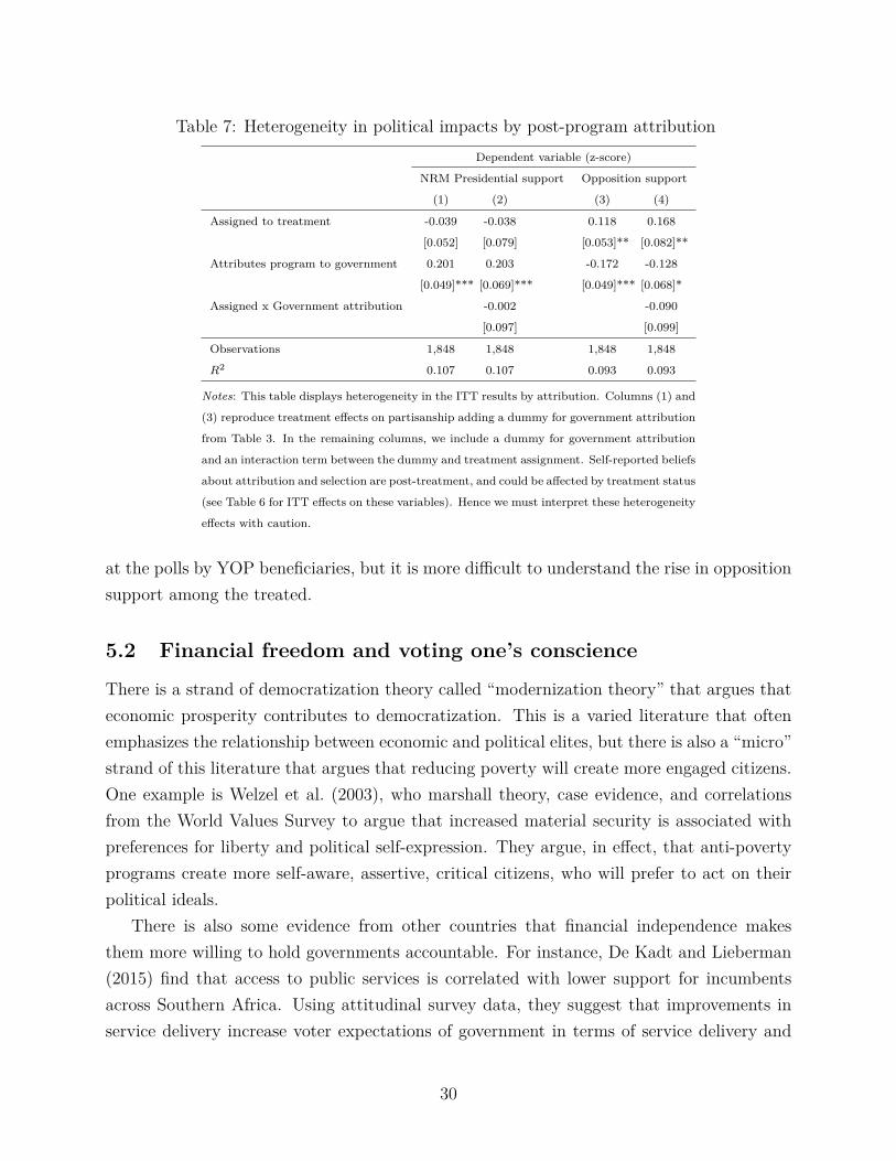
Table 7: Heterogeneity in political impacts by post-program attributionDependent variable (z-score)
NRM Presidential support Opposition support
(1) (2) (3) (4)
Assigned to treatment -0.039 -0.038 0.118 0.168
[0.052] [0.079] [0.053]** [0.082]**
Attributes program to government 0.201 0.203 -0.172 -0.128
[0.049]*** [0.069]*** [0.049]*** [0.068]*
Assigned x Government attribution -0.002 -0.090
[0.097] [0.099]
Observations 1,848 1,848 1,848 1,848
R2 0.107 0.107 0.093 0.093
Notes: This table displays heterogeneity in the ITT results by attribution. Columns (1) and
(3) reproduce treatment effects on partisanship adding a dummy for government attribution
from Table 3. In the remaining columns, we include a dummy for government attribution
and an interaction term between the dummy and treatment assignment. Self-reported beliefs
about attribution and selection are post-treatment, and could be affected by treatment status
(see Table 6 for ITT effects on these variables). Hence we must interpret these heterogeneity
effects with caution.
at the polls by YOP beneficiaries, but it is more difficult to understand the rise in oppositionsupport among the treated.
5.2 Financial freedom and voting one’s conscience
There is a strand of democratization theory called “modernization theory” that argues thateconomic prosperity contributes to democratization. This is a varied literature that oftenemphasizes the relationship between economic and political elites, but there is also a “micro”strand of this literature that argues that reducing poverty will create more engaged citizens.One example is Welzel et al. (2003), who marshall theory, case evidence, and correlationsfrom the World Values Survey to argue that increased material security is associated withpreferences for liberty and political self-expression. They argue, in effect, that anti-povertyprograms create more self-aware, assertive, critical citizens, who will prefer to act on theirpolitical ideals.
There is also some evidence from other countries that financial independence makesthem more willing to hold governments accountable. For instance, De Kadt and Lieberman(2015) find that access to public services is correlated with lower support for incumbentsacross Southern Africa. Using attitudinal survey data, they suggest that improvements inservice delivery increase voter expectations of government in terms of service delivery and
30
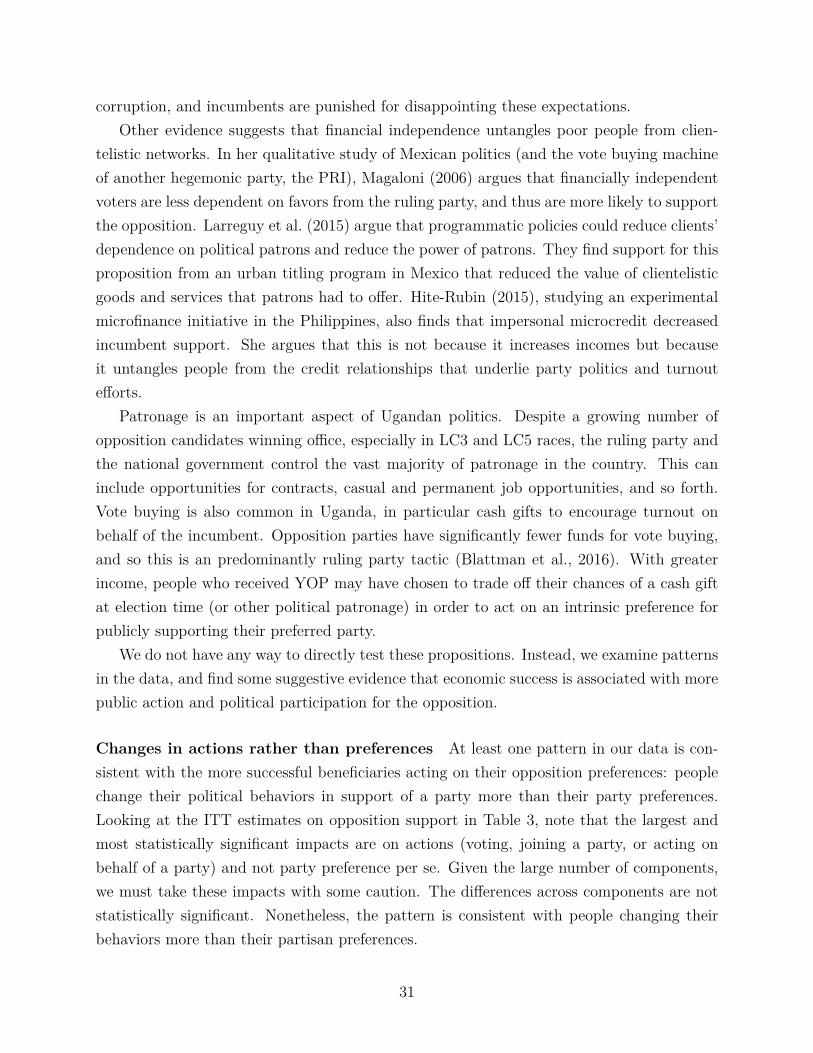
corruption, and incumbents are punished for disappointing these expectations.Other evidence suggests that financial independence untangles poor people from clien-
telistic networks. In her qualitative study of Mexican politics (and the vote buying machineof another hegemonic party, the PRI), Magaloni (2006) argues that financially independentvoters are less dependent on favors from the ruling party, and thus are more likely to supportthe opposition. Larreguy et al. (2015) argue that programmatic policies could reduce clients’dependence on political patrons and reduce the power of patrons. They find support for thisproposition from an urban titling program in Mexico that reduced the value of clientelisticgoods and services that patrons had to offer. Hite-Rubin (2015), studying an experimentalmicrofinance initiative in the Philippines, also finds that impersonal microcredit decreasedincumbent support. She argues that this is not because it increases incomes but becauseit untangles people from the credit relationships that underlie party politics and turnoutefforts.
Patronage is an important aspect of Ugandan politics. Despite a growing number ofopposition candidates winning office, especially in LC3 and LC5 races, the ruling party andthe national government control the vast majority of patronage in the country. This caninclude opportunities for contracts, casual and permanent job opportunities, and so forth.Vote buying is also common in Uganda, in particular cash gifts to encourage turnout onbehalf of the incumbent. Opposition parties have significantly fewer funds for vote buying,and so this is an predominantly ruling party tactic (Blattman et al., 2016). With greaterincome, people who received YOP may have chosen to trade off their chances of a cash giftat election time (or other political patronage) in order to act on an intrinsic preference forpublicly supporting their preferred party.
We do not have any way to directly test these propositions. Instead, we examine patternsin the data, and find some suggestive evidence that economic success is associated with morepublic action and political participation for the opposition.
Changes in actions rather than preferences At least one pattern in our data is con-sistent with the more successful beneficiaries acting on their opposition preferences: peoplechange their political behaviors in support of a party more than their party preferences.Looking at the ITT estimates on opposition support in Table 3, note that the largest andmost statistically significant impacts are on actions (voting, joining a party, or acting onbehalf of a party) and not party preference per se. Given the large number of components,we must take these impacts with some caution. The differences across components are notstatistically significant. Nonetheless, the pattern is consistent with people changing theirbehaviors more than their partisan preferences.
31
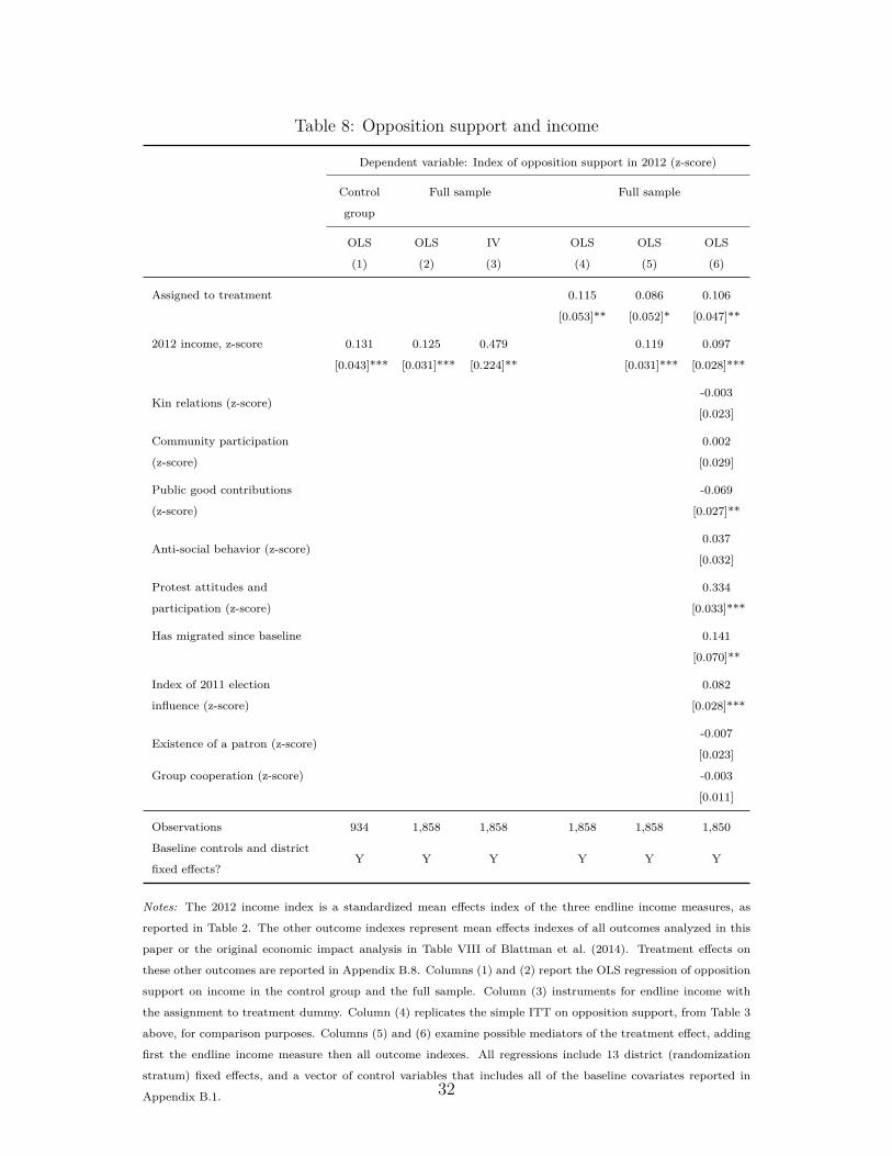
Table 8: Opposition support and income
Dependent variable: Index of opposition support in 2012 (z-score)
Control
group
Full sample Full sample
OLS OLS IV OLS OLS OLS
(1) (2) (3) (4) (5) (6)
Assigned to treatment 0.115 0.086 0.106
[0.053]** [0.052]* [0.047]**
2012 income, z-score 0.131 0.125 0.479 0.119 0.097
[0.043]*** [0.031]*** [0.224]** [0.031]*** [0.028]***
Kin relations (z-score)-0.003
[0.023]
Community participation
(z-score)
0.002
[0.029]
Public good contributions
(z-score)
-0.069
[0.027]**
Anti-social behavior (z-score)0.037
[0.032]
Protest attitudes and
participation (z-score)
0.334
[0.033]***
Has migrated since baseline 0.141
[0.070]**
Index of 2011 election
influence (z-score)
0.082
[0.028]***
Existence of a patron (z-score)-0.007
[0.023]
Group cooperation (z-score) -0.003
[0.011]
Observations 934 1,858 1,858 1,858 1,858 1,850
Baseline controls and district
fixed effects?Y Y Y Y Y Y
Notes: The 2012 income index is a standardized mean effects index of the three endline income measures, as
reported in Table 2. The other outcome indexes represent mean effects indexes of all outcomes analyzed in this
paper or the original economic impact analysis in Table VIII of Blattman et al. (2014). Treatment effects on
these other outcomes are reported in Appendix B.8. Columns (1) and (2) report the OLS regression of opposition
support on income in the control group and the full sample. Column (3) instruments for endline income with
the assignment to treatment dummy. Column (4) replicates the simple ITT on opposition support, from Table 3
above, for comparison purposes. Columns (5) and (6) examine possible mediators of the treatment effect, adding
first the endline income measure then all outcome indexes. All regressions include 13 district (randomization
stratum) fixed effects, and a vector of control variables that includes all of the baseline covariates reported in
Appendix B.1. 32
Association with wealth We also see that opposition support is correlated with wealth,and have suggestive evidence that increases in wealth are associated with increases in op-position support. Table 8 reports five OLS regressions and one instrumental variables (IV)regression, examining the relationship between the endline index of opposition support (fromTable 3) and the endline income index (from Table 2).
First, higher incomes are associated with more opposition support. In Column 1 of Table8, we report the results from a regression of opposition support on endline income for thecontrol group only, controlling for all baseline covariates (including baseline income andemployment levels). This is not a causal estimate of income on opposition support, but itdoes indicate how the variation in income that is not explained by demographics or initialincome correlates with opposition support. It is moderate in size (0.13 standard deviations)and significant at the 1% level. It is roughly similar to the correlation in the full sample, inColumn 2.37
Second, if we make the very strong assumption that all effects on opposition support aremediated through income changes (i.e. the exclusion restriction) then we can use assignmentto treatment as an instrument for the effect of income on opposition support. This IVcoefficient, in Column 3, is roughly four times as large as the OLS coefficients. It is biasedupwards by any other mediators correlated with treatment, income and opposition support.Thus we must take it with caution.
Third, alternatively we can examine the evidence on income as a mediating factor, and tryto estimate how much of the effect on opposition support is due to a rise in income.38 Column4 replicates the simple ITT on opposition support from Table 3, as a baseline reference.Column 5 adds the endline income index, while column 6 also includes 8 other potentialmechanisms (for simplicity and consistency, we include every outcome family reported ineither this paper or Blattman et al. (2014)).39
37If we omit the baseline covariates, we estimate nearly identical OLS coefficients on income (regressionsnot shown).
38See Imai et al. (2011) for a discussion of mediation analysis. They call the main assumption for causalidentification “sequential ignorability” because two ignorability assumptions are made sequentially. First,given the observed pretreatment confounders, the treatment assignment is assumed to be unconfounded—astraightforward assumption in an experiment. The second part implies that the observed mediator is ignor-able given treatment status and baseline covariates. In Column 5 this mediator is endline income, and inColumn 6 it is all endline outcome indexes, although our main interest continues to be income). The secondpart of the sequential ignorability assumption is unlikely to hold, but the analysis nonetheless provides sug-gestive information about the importance of income in mediating the effect of the YOP program on politicalbehavior.
39Six of these (family cohesion, community participation, public good contributions, anti-social behaviors,protest index, and migration) are families secondary outcomes from Blattman et al. (2014) while the othertwo (election intimation and existence of a patron) are families of secondary political variables collected forthe purpose of the paper. These encompass all secondary outcomes collected during the four year follow-up.
33
The results suggest income is a major mediating factor.40 After controlling for income in2012 (columns 4 versus 5), the treatment effect on opposition support falls by 25% (p < 0.01),while endline income is just as correlated with opposition support as in Columns 1 and 2.This suggests that a large fraction of the treatment effect we see in Column 4 is comingthrough an increase in income. When we add in the other eight mechanisms and comparecolumns 5 and 6, the treatment effect remains similar to that in column 5 (a difference of2.0 percentage points, p = 0.27). Although the coefficient on income slightly drops whenadding in these eight mechanisms (p = 0.05), the correlation between endline income andopposition support is still very high and very positive (p < 0.01). This suggests that a largeportion of the effect we observe on opposition support comes through increases in income.41
Exposure to electoral influence and patrons Finally, a reasonable (though not nec-essary) implication of the financial freedom story is that treatment should increase the re-spondent’s independence from party operators and patrons. Because we did not anticipatechanges in patron ties, we did not collect data on self-reported patronage or future expec-tations of party support. We do, however, have self-reported data on attempts to influencethe respondent during the campaign, and his perceptions of his access to patrons in times ofneed. We see some evidence that the treated were not targets of unlawful “get-out-the-vote”efforts around the 2011 election, which may suggest fewer attempts to influence their vote,but across a range of measures of election influence and intimidation we see little treatmenteffects. Also, rather than seeing treated less entangled in patron-client networks, they reportbeing more involved in patron-client networks (though not necessarily ones related to theelection). Wealth could simply improve social networks and political access. Nonetheless, itsuggests there is no simple relationship between wealth and “detangling” from patron-clientnetworks.
Table 9 reports treatment effects on instances of election influence and general patron-client ties. We do not see any significant change in most threats and incentives to voteone way or the other. Treated people were, however, about half as likely to be taken tothe poll on election day—a fall of 2 percentage points relative to a mean of 4 percentagepoints in the control group. The mean is low because such voter mobilization on election
40Though it may not satisfy the exclusion restriction assumed in Column 3.41While other endline indexes are significantly correlated with opposition support, this is not sufficient to
mediate the treatment effect on income. To do so, they must also be correlated with treatment, and noneare correlated with both treatment and the outcome to a significant degree other than income. This is whywe see no fall in the treatment coefficient when these other variables are added to Column 6. We expand onthese points, and illustrate treatment effects, in Appendix B.7, where we perform a more formal mediationanalysis based off of Keele et al. (2015). Consistent with the findings reported here, we estimate that almost25 percent of the treatment effect comes from the measured increase in income—large compared to othermediation analyses of this nature.
34

day is outlawed in Uganda. A mean effects index of election influence shows no statisticallysignificant impact.
We find that the program has a positive and statistically significant effect on the exis-tence of a patron—a family member, “big man”, or politician— the respondent feels he orshe can go to when in need of something. It is unclear whether these are political patronswho mobilize people for political support, as we do not see a statistically significant rise inone of these patrons trying to influence their political behavior during the election. Only22% of respondents reported that a patron tried to influence their actions, and this increasedby 2 percentage points (not significant) with treatment. We only asked about attempts toinfluence, not success, and so this does not rule out the possibility that the treated disen-tangled themselves from election pressure and patronage. But nor is the pattern consistentwith the financial freedom story. One interpretation is that business activities and wealthstrengthen general financial and social networks, including political networks. Another isthat active and public support for a political party (in this case, opposition parties) createspolitical connections.
6 Conclusions
We analyze the political consequences of a large scale, successful employment program inUganda. We find that, rather than rewarding the incumbent ruling party for this program-matic policy, treated young people are less likely to vote for the President and are morelikely to engage in campaigning for the opposition. We show that the lack of reward for theincumbent is likely not coming from a lack of attributing the program to the incumbent,since a majority of beneficiaries do in fact attribute the program to the government. We seesuggestive evidence that opposition support is associated with wealth increases, and this isconsistent with a story where more successful youth are able to vote their conscience ratherthan succumb to incentives or pressures to support the ruling party.
Existing evidence points in the opposite direction, that incumbents are rewarded forpatronage and programmatic policies, and so it is possible that this result is unique to Ugandaor even this context. We would expect context to play a huge role in any treatment effectof a policy on political behavior, and any number of factors could influence the recipient’sreaction to YOP: the nature of the program, the issues at play in this election, or the fact thatthese are largely first- and second-time voters. For example, many of the other programs thathave been studied examine repeated cash transfers over time, rather than one-time grants,allowing political parties to claim credit repeatedly. These program features could changethe political interpretation and effects.
35

Table 9: Program impacts on other political outcomesFull sample
(1) (2) (3) (4)
Control ITT, with controls
Dependent variable in 2012 Mean Coeff. Std. Err. N
Index of 2011 election influence (z-score) 0.03 0.04 [.05] 1,858
Was offered money in exchange for vote (0-3) 0.52 0.06 [.048] 1,857
Was threatened during campaign (0-3) 0.23 0.04 [.034] 1,857
Was intimidated during campaign (0-3) 0.90 -0.01 [.057] 1,857
Was taken to the poll on election day 0.04 -0.02 [.008]** 1,858
Any of patrons tried to influence you 0.22 0.02 [.019] 1,839
Existence of a patron (z-score) -0.09 0.14 [.05]*** 1,850
There is a family member he can go to if in need 0.39 0.04 [.024]* 1,844
There is a big man he can go to if in need 0.29 0.04 [.024]* 1,840
There is politician he can go to if in need 0.23 0.07 [.021]*** 1,837
Any of patrons tried to influence you during 2011 election 0.22 0.02 [.019] 1,839
Notes: Column (1) reports the control group mean, weighted by the inverse probability of selection into
each endline sample. Columns (2)-(3) report the estimated intent-to-treat (ITT) coefficient and standard
error at endline. Standard errors are heteroskedastic-robust and clustered by group. The number of
observations in Column 4 may differ from the total number of people survey (1,868) because a small
number of people, typically less than 1–2%, declined to answer the political questions.We calculate the
ITT via a weighted least squares regression of the dependent variable on a program assignment indicator,
13 district (randomization stratum) fixed effects, and a vector of control variables that includes all of the
baseline covariates reported in Appendix B.1.
36
Prominent reviews of the literature on distributive politics have called attention to incom-plete evidence and possible publication bias. For example, Golden and Min (2013) note that,“it is hard not to suspect that the cases that are studied are often selected precisely becausethey display prima facie evidence of political distortions in allocative decisions” (p.86). Theygo on to note that “either that the study of allocations is incomplete, a problem identifiedby Cox (2010), or that the cumulative results of this research agenda are biased—or both.”
Our hypothesis—that the program, by creating wealth, led to the financial freedom tovote one’s true political preferences—is just that, a hypothesis. We do not have the dataor design to test the mechanism at work. Nonetheless, it accords with the conclusions ofpolitical scientists in contexts as different as Mexico and the Philippines, and strikes usas an important hypothesis for the literature, and future experiments, to take seriously.Relatively few employment and anti-poverty program evaluations collect data on programattribution and resulting political attitudes and behavior. Most regions, however, offer off-the-shelf political survey questionnaires with nationally representative data for comparison(e.g. Afrobarometer, Latinobarometer, etc.). Past experimental anti-poverty programs arealso fodder for downstream studies of political impacts. We hope this paper motivates suchdata collection and addresses the gap in evidence, to investigate the idea that the escapefrom poverty might be associated with political freedoms.
References
Achen, C. H. and L. M. Bartels (2004). Blind Retrospection: Electoral Responses to Drought,Flu, and Shark Attacks. Working paper . 2, 20
Ashworth, S., E. B. de Mesquita, and A. Freidenberg (2016). Learning About Voter Ratio-nality. Working paper . 21
Baez, J. E., A. Camacho, E. Conover, and R. A. Zarate (2012). Conditional cash transfers,political participation, and voting behavior. Working paper . 2
Banerjee, A. V. (2013). Microcredit Under the Microscope: What Have We Learned in thePast Two Decades, and What Do We Need to Know? Annual Review of Economics 5 (1),487–519. 6
Banerjee, A. V. and E. Duflo (2011). Poor economics: A radical rethinking of the way tofight global poverty. New York: Public Affairs. 8
37
Banerjee, A. V., E. Duflo, R. Glennerster, and C. Kinnan (2013). The Miracle of Micro-finance? Evidence from a Randomized Evaluation. Unpublished working paper, MIT .8
Banerjee, A. V., E. Duflo, N. Goldberg, D. Karlan, R. Osei, W. Parienté, J. Shapiro,B. Thuysbaert, and C. Udry (2015). A Multi-faceted Program Causes Lasting Progressfor the Very Poor: Evidence from Six Countries. Science. 6, 8
Besley, T. J. and T. Persson (2011). Pillars of Prosperity: The Political Economics ofDevelopment Clusters. Princeton: Princeton University Press. 3
Blattman, C., J. Annan, E. P. Green, and J. Jamison (2013). The returns to cash andmicroenterprise support among the ultra-poor: A field experiment. Working paper . 6
Blattman, C., N. Fiala, and S. Martinez (2014). Generating skilled employment in developingcountries: Experimental evidence from uganda. Quarterly Journal of Economics 129 (2),697–752. 1, 4, 6, 17, 19, 32, 33
Blattman, C., H. Larreguy, B. Marx, and O. Reid (2016). A Market Equilibrium Approachto Reduce the Incidence of Vote-Buying: Evidence from Uganda. Working paper . 31
Blattman, C. and L. Ralston (2015). Generating employment in poor and fragile states: Areview of the evidence from labor market and entrepreneurship programs. Working paper .8, 19
Casaburi, L. and U. Troiano (2015, October). Ghost-House Busters: the Electoral Responseto a Large Anti–Tax Evasion Program. The Quarterly Journal of Economics, qjv041. 20
De Kadt, D. and E. S. Lieberman (2015). Do Citizens Reward Good Service? Voter Re-sponses to Basic Service Provision in Southern Africa. Working paper . 5, 30
De La O, A. (2013). Do conditional cash transfers affect electoral behavior? evidence froma randomized experiment in mexico. American Journal of Political Science 57 (1), 1–14.2
de Mel, S., D. J. McKenzie, and C. Woodruff (2008). Returns to Capital in Microenterprises:Evidence from a Field Experiment. Quarterly Journal of Economics 123, 1329–1372. 4. 6
Diaz-Cayeros, A., F. Estevez, and B. Magaloni (2016). Strategies of Vote Buying: Democracy,Clientelism and Poverty Relief in Mexico. New York: Cambridge University Press. 20
38

Dietrich, S. and M. S. Winters (2014). Foreign Aid and Government Legitimacy. Workingpaper . 5
Fafchamps, M., D. J. McKenzie, S. Quinn, and C. Woodruff (2014). When is capitalenough to get female microenterprises growing? Evidence from a randomized experimentin Ghana. Journal of Development Economics. 6
Ferguson, J. (1990). The anti-politics machine:" development," depoliticization, and bureau-cratic power in Lesotho. Cambridge: Cambridge University Press. 3
Fiorina, M. P. (1976). The voting decision: instrumental and expressive aspects. The Journalof Politics 38, 390–413. 2. 20
Golden, M. and B. Min (2013). Distributive Politics Around the World. Annual Review ofPolitical Science 16 (1), 73–99. 2, 37
Gomez, B. T. and J. M. Wilson (2001, October). Political Sophistication and EconomicVoting in the American Electorate: A Theory of Heterogeneous Attribution. AmericanJournal of Political Science 45 (4), 899–914. 2
Government of Uganda (2007). National Peace, Recovery and Development Plan for North-ern Uganda: 2006-2009. Technical report, Government of Uganda, Kampala. 6, 7
Green, E. (2010). Patronage, district creation, and reform in uganda. Studies in comparativeinternational development 45 (1), 83–103. 10
Green, E. (2011). Patronage as institutional choice: evidence from rwanda and uganda.Comparative politics 43 (4), 421–438. 10
Grossman, G. and J. I. Lewis (2013). Administrative unit proliferation. American PoliticalScience Review. 10
Guiteras, R. and A. M. Mobarak (2014). Does Development Aid Undermine Political Ac-countability? Leader and Constituent Responses to a Large-Scale Intervention. Workingpaper . 5
Haushofer, J. and J. Shapiro (2013). Welfare Effects of Unconditional Cash Transfers: Evi-dence from a Randomized Controlled Trial in Kenya. Working paper . 6
Hausmann, R., B. Cunningham, J. Matovu, R. Osire, and K. Wyett (2014). How shoulduganda grow? 7
39
Healy, A. J., N. Malhotra, and C. H. Mo (2010, July). Irrelevant events affect voters’evaluations of government performance. Proceedings of the National Academy of Sci-ences 107 (29), 12804–12809. 2, 20
Hickey, S. (2005). The politics of staying poor: exploring the political space for povertyreduction in Uganda. World development 33 (6), 995–1009. 7
Hickey, S. (2013). Beyond the poverty agenda? insights from the new politics of developmentin uganda. World Development 43, 194–206. 7, 11
Hite-Rubin, N. (2015). Including the Other Half: How financial modernization disruptspatronage politics. Working paper . 5, 31
Imai, K., L. Keele, D. Tingley, and T. Yamamoto (2011). Unpacking the Black Box of Causal-ity: Learning about Causal Mechanisms from Experimental and Observational Studies.American Political Science Review 105, 765–789. 4. 33
Imai, K., G. King, and C. V. Rivera (2016). Do Nonpartisan Programmatic Policies HavePartisan Electoral Effects? Evidence from Two Large Scale Randomized Experiments.Working paper . 2
Jones, B. (2009, May). The two sides of uganda. The Guardian. 7
Kavuma, R. M. (2010, January). Nusaf: Developing northern Uganda. The Guardian. 10
Keele, L., D. Tingley, and T. Yamamoto (2015). Identifying mechanisms behind policy inter-ventions via causal mediation analysis. Journal of Policy Analysis and Management 34 (4),937–963. 34, xv, xvi
Kinder, D. R. and D. R. Kiewiet (1981, April). Sociotropic Politics: The American Case.British Journal of Political Science 11 (2), 129–161. 2
Kitschelt, H. and S. I. Wilkinson (2007). Patrons, clients and policies: Patterns of democraticaccountability and political competition. Cambridge University Press. 2
Kramer, G. H. (1971). Short-term Fluctuations in U.S. Voting Behavior: 1896-1964. TheAmerican Political Science Review 65, 131–43. 1. 20
Larreguy, H., J. Marshall, and L. Trucco (2015). Breaking clientelism or rewarding incum-bents? Evidence from an urban titling program in Mexico. 5, 20, 31
Magaloni, B. (2006). Voting for autocracy: Hegemonic party survival and its demise inMexico. Cambridge University Press Cambridge. 5, 31
40
Magaloni, B., E. Min, and J. Chu (2013). Autocracies of the World, 1950-2012 (Version 1.0).Dataset. 6
Manacorda, M., E. Miguel, and A. Vigorito (2011). Government Transfers and PoliticalSupport. American Economic Journal: Applied Economics 3 (3), 1–28. 2, 20
McKenzie, D. J. and C. Woodruff (2012). What are we learning from business training andentrepreneurship evaluations around the developing world? Working paper . 6
Moss, T. J., G. Pettersson, and N. Van de Walle (2006). An aid-institutions paradox? Areview essay on aid dependency and state building in sub-Saharan Africa. Center forGlobal Development Working Paper (74), 11–05. 3
Mwenda, A. M. and R. Tangri (2005). Patronage politics, donor reforms, and regime con-solidation in uganda. African affairs 104 (416), 449–467. 7
Ojwee, D. (2008, August). Gulu probes corruption in NUSAF. The New Vision. 10
Pop-Eleches, C. and G. Pop-Eleches (2012). Targeted government spending and politicalpreferences. Quarterly Journal of Political Science 7 (3), 285–320. 2
Schober, G. S. (2016). Conditional Cash Transfers and Electoral Behavior: ExperimentalEvidence from Mexico. Working Paper . 2, 20
Tangri, R. and A. M. Mwenda (2008). Elite corruption and politics in Uganda. Common-wealth & Comparative Politics 46 (2), 177–194. 3
Thachil, T. (2011). Embedded mobilization: nonstate service provision as electoral strategyin India. World Politics 63 (03), 434–469. 3
Tripp, A. M. (2010). Museveni’s Uganda: paradoxes of power in a hybrid regime. LynneRienner Publishers. 6
Welzel, C., R. Inglehart, and H.-D. Kligemann (2003, May). The theory of human develop-ment: A cross-cultural analysis. European Journal of Political Research 42 (3), 341–379.5, 30
Westfall, P. H. and S. S. Young (1993). Resampling-based multiple testing: Examples andmethods for p-value adjustment, Volume 279. John Wiley & Sons. 23
Zucco, C. (2013). When payouts pay off: Conditional cash transfers and voting behavior inbrazil 2002–10. American Journal of Political Science 57 (4), 810–822. 20
41
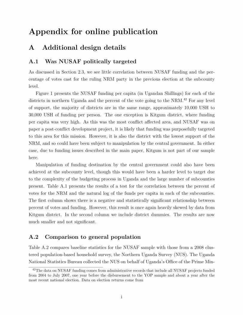
Appendix for online publication
A Additional design details
A.1 Was NUSAF politically targeted
As discussed in Section 2.3, we see little correlation between NUSAF funding and the per-centage of votes cast for the ruling NRM party in the previous election at the subcountylevel.
Figure 1 presents the NUSAF funding per capita (in Ugandan Shillings) for each of thedistricts in northern Uganda and the percent of the vote going to the NRM.42 For any levelof support, the majority of districts are in the same range, approximately 10,000 USH to30,000 USH of funding per person. The one exception is Kitgum district, where fundingper capita was very high. As this was the most conflict affected area, and NUSAF was onpaper a post-conflict development project, it is likely that funding was purposefully targetedto this area for this mission. However, it is also the district with the lowest support of theNRM, and so could have been subject to manipulation by the central government. In eithercase, due to funding issues described in the main paper, Kitgum is not part of our samplehere.
Manipulation of funding destination by the central government could also have beenachieved at the subcounty level, though this would have been a harder level to target dueto the complexity of the budgeting process in Uganda and the large number of subcountiespresent. Table A.1 presents the results of a test for the correlation between the percent ofvotes for the NRM and the natural log of the funds per capita in each of the subcounties.The first column shows there is a negative and statistically significant relationship betweenpercent of votes and funding. However, this result is once again heavily skewed by data fromKitgum district. In the second column we include district dummies. The results are nowmuch smaller and not significant.
A.2 Comparison to general population
Table A.2 compares baseline statistics for the NUSAF sample with those from a 2008 clus-tered population-based household survey, the Northern Uganda Survey (NUS). The UgandaNational Statistics Bureau collected the NUS on behalf of Uganda’s Office of the Prime Min-
42The data on NUSAF funding comes from administrative records that include all NUSAF projects fundedfrom 2004 to July 2007, one year before the disbursement to the YOP sample and about a year after themost recent national election. Data on election returns come from
i
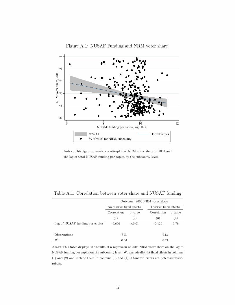
Figure A.1: NUSAF Funding and NRM voter share
0.2
.4.6
.81
NR
M v
oter
shar
e, 2
006
6 8 10 12NUSAF funding per capita, log UGX
95% CI Fitted values% of votes for NRM, subcounty
Notes: This figure presents a scatterplot of NRM voter share in 2006 and
the log of total NUSAF funding per capita by the subcounty level.
Table A.1: Correlation between voter share and NUSAF fundingOutcome: 2006 NRM voter share
No district fixed effects District fixed effects
Correlation p-value Correlation p-value
(1) (2) (3) (4)
Log of NUSAF funding per capita -0.660 <0.01 -0.120 0.78
Observations 313 313
R2 0.04 0.27
Notes: This table displays the results of a regression of 2006 NRM voter share on the log of
NUSAF funding per capita on the subcounty level. We exclude district fixed effects in columns
(1) and (2) and include them in columns (3) and (4). Standard errors are heteroskedastic-
robust.
ii

ister, in part to help the government assess the impacts of NUSAF on the north. The NUSwas conducted in all NUSAF districts and focused on consumption, labor market activity,and health and education in the household. NUS sampling probabilities are estimates of theprobability of being sampled in the full northern population.
A.3 Two-stage surveys and response rates
Both endline surveys (2010 and 2012) were rolled out in two phases In Phase 1, we attemptedto interview all 2,677 people in their last known location. In 2010, 37% were not found intheir last know location, rising to 39% in 2012, and so they became eligible for tracking inPhase 2. In Phase 2, we selected a random sample of the unfound—53% in 2010 and 38.5%in 2012—stratifying by district and by the proportion unfound in the group for in-depthtracking. For this subset of unfound groups, we made three attempts to find them in theirnew locations and found 75% of them in 2010 and 59% in 2012. In the analysis, groups areweighted to account for this two-stage process. Those found in Phase 1 receive unit weight,those selected for Phase 2 tracking are weighted by the inverse of their selection probability,while those not selected for Phase 2 tracking are dropped. We have no reports of surveyrefusal, and no reward was offered for survey completion. See table A.3 for a more detailedpresentation of effective response rates.
A.4 Survey experiment
To manipulate participant ideas about the implementation of the program, we conducted asurvey experiment during the four-year endline. The goal of the survey experiment was tomanipulate respondents’ ideas about who was behind the implementation of the program(World Bank versus the government) and how participants were selected (randomly selectedor nominated by the LC V). Individuals were randomized into one of five groups and in eachgroup the introductory script of the survey varied along these two dimensions.
1. World Bank, Random. These surveys emphasized that the program was principallymade possible by the action of the World Bank and that the groups were selectedrandomly to receive funding.
2. World Bank, LC V. These surveys emphasized that the program was principallymade possible by the action of the World Bank, but groups were selected by the NUSAFdistrict technical officer (NDTO) under the supervision of the LC V Chairperson.
3. Government, Random. These surveys emphasized that the program was principally
iii

Table A.2: Comparison to other population-based surveysSurvey
YOP sample Afrobarometer
Covariate 2008 2012 2008 2010 2011 2012
(1) (2) (3) (4) (5) (6)
Age 24.96 25.03 33.49 33.98 35.38 36.13
Female 0.33 0.33 0.50 0.50 0.50 0.50
Education
None 0.03 0.04 0.10 0.16 0.19 0.18
Primary 0.45 0.47 0.44 0.47 0.36 0.42
Secondary 0.46 0.37 0.45 0.35 0.43 0.37
University 0.05 0.11 0.01 0.01 0.02 0.02
Post-Graduate 0.00 0.00 0.00 0.00 0.00 0.00
Religion
None 0.00 0.02 0.01 0.00
Catholic 0.44 0.45 0.85 0.83 0.80 0.85
Muslim 0.11 0.11 0.03 0.05 0.09 0.10
Pentecostal 0.15 0.15 0.09 0.08 0.08 0.05
Protestant 0.30 0.28 0.00 0.01 0.00 0.00
Other 0.01 0.01 0.03 0.02 0.02 0.00
Ethnic group
Acholi 0.01 0.00 0.00 0.00 0.01
Alur 0.03 0.03 0.08 0.07 0.04
Ateso 0.19 0.13 0.18
Karamojong 0.07 0.07 0.00 0.00 0.18
Langi 0.35 0.35 0.47 0.29 0.24
Lugbara 0.12 0.12 0.06 0.12 0.18
Madi 0.08 0.08 0.14 0.07 0.07
Other 0.15 0.16 0.06 0.32 0.11
Member of a political party 0.50 0.65 0.68
Worked for a political party 0.38 0.46 0.46 0.26
Strongly like or Like DP 0.10 0.09 0.06
Strongly like or Like FDC 0.22 0.22 0.25
Strongly like or Like UPC 0.22 0.24 0.24
Strongly like or Like NRM 0.80 0.65 0.67
Observations 2,598 1,868 447 504 448 576
Notes: This table compares the YOP-sample to the Afrobarometer survey. Afrobarom-
eter responses limited to the districts in the YOP sample.
iv
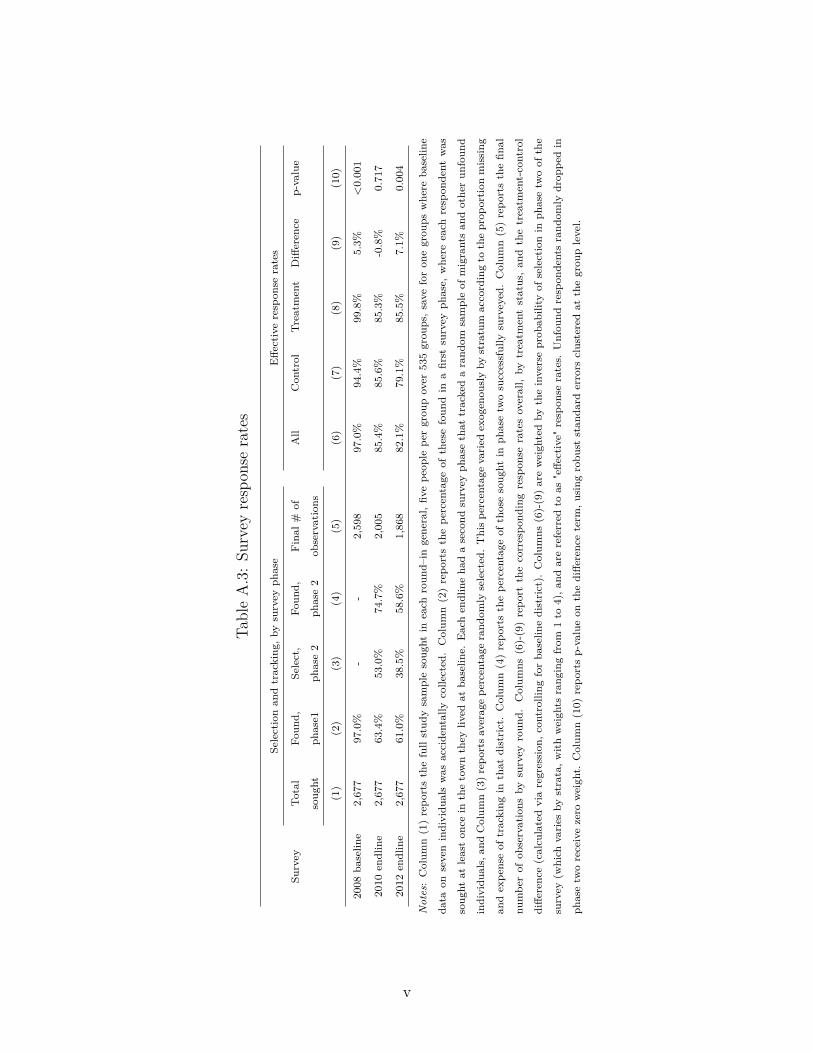
TableA.3:Su
rvey
respon
serates
Selectionan
dtracking
,bysurvey
phase
Effe
ctiverespon
serates
Survey
Total
soug
ht
Foun
d,
phase1
Select,
phase2
Foun
d,
phase2
Final
#of
observations
All
Con
trol
Treatm
ent
Difference
p-value
(1)
(2)
(3)
(4)
(5)
(6)
(7)
(8)
(9)
(10)
2008
baselin
e2,677
97.0%
--
2,598
97.0%
94.4%
99.8%
5.3%
<0.001
2010
endline
2,677
63.4%
53.0%
74.7%
2,005
85.4%
85.6%
85.3%
-0.8%
0.717
2012
endline
2,677
61.0%
38.5%
58.6%
1,868
82.1%
79.1%
85.5%
7.1%
0.004
Not
es:Colum
n(1)repo
rtsthefullstud
ysamplesoug
htin
each
roun
d–in
general,fiv
epe
ople
pergrou
pover
535grou
ps,s
aveforon
egrou
pswhere
baselin
e
data
onsevenindividu
alswas
accidentally
collected.Colum
n(2)repo
rtsthepe
rcentage
ofthesefoun
din
afirst
survey
phase,
where
each
respon
dent
was
soug
htat
leaston
cein
thetownthey
lived
atba
selin
e.Eachendlineha
dasecond
survey
phasethat
trackedarand
omsampleof
migrantsan
dotherun
foun
d
individu
als,an
dColum
n(3)repo
rtsaveragepe
rcentage
rand
omly
selected.Thispe
rcentage
varied
exogenou
slyby
stratum
accordingto
theprop
ortion
missing
andexpe
nseof
tracking
inthat
district.Colum
n(4)repo
rtsthepe
rcentage
ofthosesoug
htin
phasetw
osuccessfully
surveyed.Colum
n(5)repo
rtsthefin
al
numbe
rof
observations
bysurvey
roun
d.Colum
ns(6)-(9)repo
rtthecorrespo
ndingrespon
seratesoverall,by
treatm
entstatus,an
dthetreatm
ent-control
diffe
rence(calculatedviaregression
,con
trollin
gforba
selin
edistrict).
Colum
ns(6)-(9)areweigh
tedby
theinverseprob
ability
ofselectionin
phasetw
oof
the
survey
(which
varies
bystrata,w
ithweigh
tsrang
ingfrom
1to
4),a
ndarereferred
toas
"effe
ctive"
respon
serates.
Unfou
ndrespon
dentsrand
omly
drop
pedin
phasetw
oreceivezero
weigh
t.Colum
n(10)
repo
rtsp-valueon
thediffe
renceterm
,using
robu
ststan
dard
errors
clusteredat
thegrou
plevel.
v

Table A.4: Survey experiment resultsFirst stage attribution First stage selection
Government World Bank Random Not random
(1) (2) (3) (4)
Attribute program to: Believes selection was
Government -0.03 -0.04 Random 0.03 0.02
[.031] [.030] [.020] [.020]
World Bank 0.05 0.04 Not random -0.03 -0.06
[.029]* [.028] [.032] [.029]**
Notes: This table displays ITT results from our survey experiment. In column (1), we regress program attribution
on an indicator for completing a survey where the introduction said the government was behind the program
plus covariates and block fixed effects. In column (2), we include an indicator for completing a survey that said
the World Bank was behind the program. In column (3), we regress believe in selection process on an indicator
for completing a survey where the introduction said selection was random plus covariates and block fixed effects.
In column (4), we include an indicator for completing a survey that said selection was not random.
made possible by the action of the government and that the groups were selectedrandomly to receive funding.
4. Government, LC V. These surveys emphasized that the program was principallymade possible by the action of the government, but groups were selected by the NDTOunder the supervision of the LC V Chairperson.
5. Neutral. None of the above information was presented.
Table A.4 displays the results of our survey experiment. The results show that the experimentwas not successful: individuals who were told the government was behind the program were5 percentage points more likely to believe the World Bank funded the program. Similarly,individuals who were told selection was not random were 6 percentage points less likely tobelieve selection was not random.
B Additional analysis
B.1 Baseline balance
Table B.1 displays the results of a regression of treatment on each baseline covariate, con-trolling for district fixed effects and clustering standard errors by group.
vi
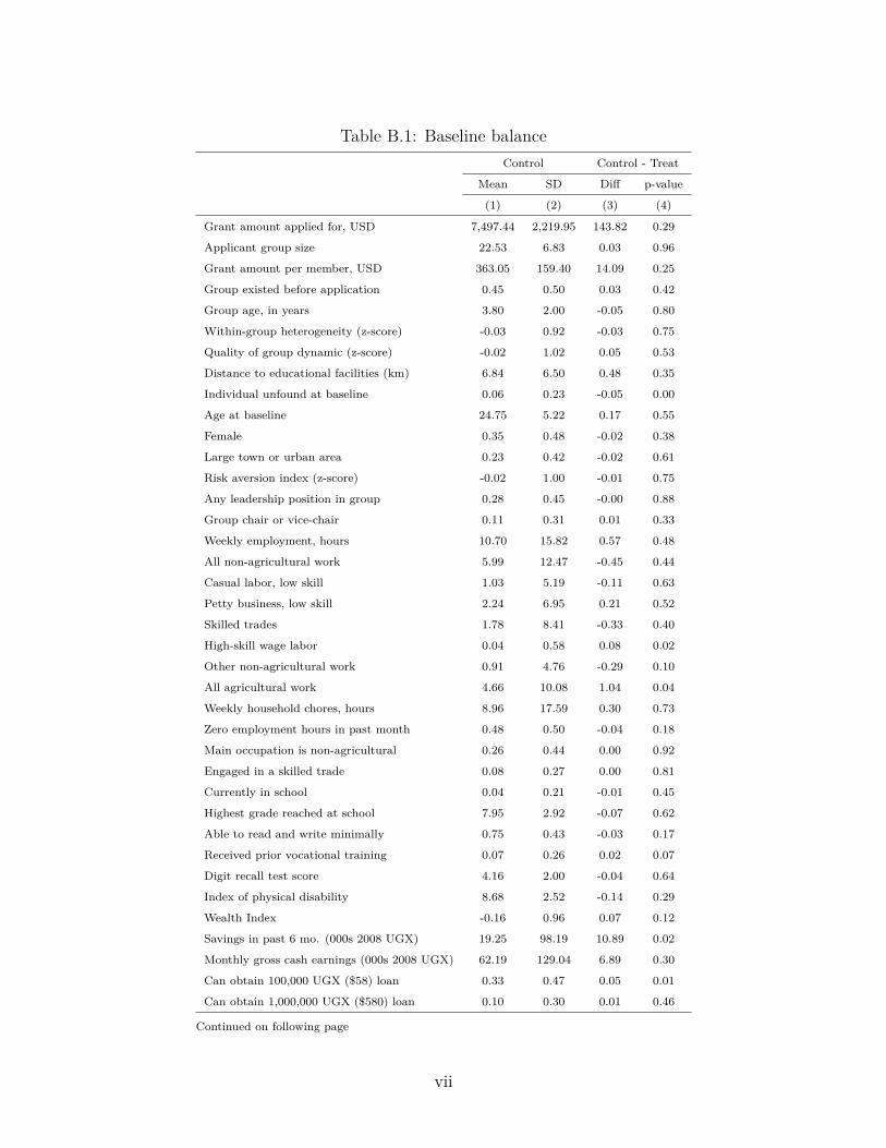
Table B.1: Baseline balanceControl Control - Treat
Mean SD Diff p-value
(1) (2) (3) (4)
Grant amount applied for, USD 7,497.44 2,219.95 143.82 0.29
Applicant group size 22.53 6.83 0.03 0.96
Grant amount per member, USD 363.05 159.40 14.09 0.25
Group existed before application 0.45 0.50 0.03 0.42
Group age, in years 3.80 2.00 -0.05 0.80
Within-group heterogeneity (z-score) -0.03 0.92 -0.03 0.75
Quality of group dynamic (z-score) -0.02 1.02 0.05 0.53
Distance to educational facilities (km) 6.84 6.50 0.48 0.35
Individual unfound at baseline 0.06 0.23 -0.05 0.00
Age at baseline 24.75 5.22 0.17 0.55
Female 0.35 0.48 -0.02 0.38
Large town or urban area 0.23 0.42 -0.02 0.61
Risk aversion index (z-score) -0.02 1.00 -0.01 0.75
Any leadership position in group 0.28 0.45 -0.00 0.88
Group chair or vice-chair 0.11 0.31 0.01 0.33
Weekly employment, hours 10.70 15.82 0.57 0.48
All non-agricultural work 5.99 12.47 -0.45 0.44
Casual labor, low skill 1.03 5.19 -0.11 0.63
Petty business, low skill 2.24 6.95 0.21 0.52
Skilled trades 1.78 8.41 -0.33 0.40
High-skill wage labor 0.04 0.58 0.08 0.02
Other non-agricultural work 0.91 4.76 -0.29 0.10
All agricultural work 4.66 10.08 1.04 0.04
Weekly household chores, hours 8.96 17.59 0.30 0.73
Zero employment hours in past month 0.48 0.50 -0.04 0.18
Main occupation is non-agricultural 0.26 0.44 0.00 0.92
Engaged in a skilled trade 0.08 0.27 0.00 0.81
Currently in school 0.04 0.21 -0.01 0.45
Highest grade reached at school 7.95 2.92 -0.07 0.62
Able to read and write minimally 0.75 0.43 -0.03 0.17
Received prior vocational training 0.07 0.26 0.02 0.07
Digit recall test score 4.16 2.00 -0.04 0.64
Index of physical disability 8.68 2.52 -0.14 0.29
Wealth Index -0.16 0.96 0.07 0.12
Savings in past 6 mo. (000s 2008 UGX) 19.25 98.19 10.89 0.02
Monthly gross cash earnings (000s 2008 UGX) 62.19 129.04 6.89 0.30
Can obtain 100,000 UGX ($58) loan 0.33 0.47 0.05 0.01
Can obtain 1,000,000 UGX ($580) loan 0.10 0.30 0.01 0.46
Continued on following page
vii
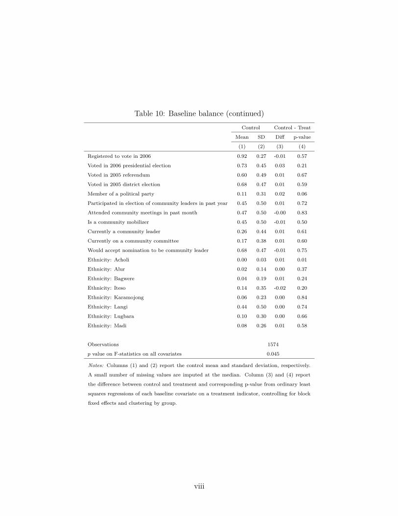
Table 10: Baseline balance (continued)Control Control - Treat
Mean SD Diff p-value
(1) (2) (3) (4)
Registered to vote in 2006 0.92 0.27 -0.01 0.57
Voted in 2006 presidential election 0.73 0.45 0.03 0.21
Voted in 2005 referendum 0.60 0.49 0.01 0.67
Voted in 2005 district election 0.68 0.47 0.01 0.59
Member of a political party 0.11 0.31 0.02 0.06
Participated in election of community leaders in past year 0.45 0.50 0.01 0.72
Attended community meetings in past month 0.47 0.50 -0.00 0.83
Is a community mobilizer 0.45 0.50 -0.01 0.50
Currently a community leader 0.26 0.44 0.01 0.61
Currently on a community committee 0.17 0.38 0.01 0.60
Would accept nomination to be community leader 0.68 0.47 -0.01 0.75
Ethnicity: Acholi 0.00 0.03 0.01 0.01
Ethnicity: Alur 0.02 0.14 0.00 0.37
Ethnicity: Bagwere 0.04 0.19 0.01 0.24
Ethnicity: Iteso 0.14 0.35 -0.02 0.20
Ethnicity: Karamojong 0.06 0.23 0.00 0.84
Ethnicity: Langi 0.44 0.50 0.00 0.74
Ethnicity: Lugbara 0.10 0.30 0.00 0.66
Ethnicity: Madi 0.08 0.26 0.01 0.58
Observations 1574
p value on F-statistics on all covariates 0.045
Notes: Columns (1) and (2) report the control mean and standard deviation, respectively.
A small number of missing values are imputed at the median. Column (3) and (4) report
the difference between control and treatment and corresponding p-value from ordinary least
squares regressions of each baseline covariate on a treatment indicator, controlling for block
fixed effects and clustering by group.
viii

B.2 Correlates of attrition
Table B.2 examines baseline correlates of attrition. We regress an indicator for attritionon all baseline covariates including district fixed effects. Those who are younger, more riskaverse or work as casual laborers are more likely to attrit. Since attrition is higher amongthe young and initially poorer, the average impact of treatment is predicted to be higher.At the same time, the more literate are more likely to be unfound and so this could depresstheir predicted returns from a grant.
B.3 Sensitivity of baseline balance to baseline non-response
Table B.3 looks at the sensitivity of randomization balance to alternate values for the miss-ing control groups. The table examines four baseline covariates displaying randomizationimbalance at baseline: durable assets, prior vocational training, ability to obtain a 100,000UGX loan, and savings in the past 6 months. All covariates are standardized and missingdata in the treatment group are imputed to the mean, or zero. However, missing controlgroup data are imputed to the mean (zero) plus 0.05, 0.10, 0.15, 0.20, or 0.25 SD of thecovariate, thus gradually increasing the values of the covariates in the control group towardsbalance. In general, imputed values of 0.10 to 0.20 SD are sufficient to bring the regressiondifferences to zero.
B.4 Robustness
We perform two sets of additional treatment analyses. Our first robustness check is to alter-native specifications, which is displayed in Table B.4. We test four alternate specifications.In the first, we drop all controls and only include randomization block fixed effects. In ournext one, we add only demographic covariates. Next we add all human and physical capitalcontrols. Our final specification includes all covariates but uses randomization inference tocalculate the standard errors. As shown in the table, our results are robust to these alternatespecifications.
Our second robustness check is to alternative attrition scenarios. We impute outcomevalues for unfound individuals at different points of the observed outcome distribution. Themost extreme bound, from Manski 1990, imputes the minimum value for unfound treatedmembers and the maximum for unfound controls. Following Karlan et al. 2015, we alsocalculate less extreme bounds by imputing relatively high values of the dependent variablesfor missing control group members, and relatively low values for missing treatment group
ix
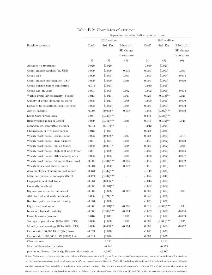
Table B.2: Correlates of attritionDependent variable: Indicator for attrition
2010 endline 2012 endline
Baseline covariate Coeff. Std. Err. Effect of 1
SD change
in covariate
Coeff. Std. Err. Effect of 1
SD change
in covariate
(1) (2) (3) (4) (5) (6)
Assigned to treatment 0.020 [0.020] . -0.050 [0.023] .
Grant amount applied for, USD 0.000 [0.000] -0.030 0.000 [0.000] 0.000
Group size 0.000 [0.005] 0.003 -0.005 [0.004] -0.034
Grant amount per member, USD 0.000 [0.000] 0.035 0.000 [0.000] -0.010
Group existed before application -0.016 [0.024] . -0.030 [0.025] .
Group age, in years 0.001 [0.005] 0.002 -0.002 [0.006] -0.003
Within-group heterogeneity (z-score) 0.013 [0.011] 0.013 0.026 [0.013]** 0.026
Quality of group dynamic (z-score) 0.008 [0.013] 0.008 -0.009 [0.016] -0.009
Distance to educational facilities (km) 0.002 [0.002] 0.015 0.000 [0.003] -0.002
Age at baseline -0.003 [0.002]* -0.018 -0.006 [0.002]*** -0.030
Large town/urban area 0.081 [0.030]*** . 0.143 [0.036]*** .
Risk aversion index (z-score) 0.039 [0.011]*** 0.039 0.046 [0.012]** 0.046
Management committee member -0.044 [0.018]** . -0.042 [0.024] .
Chairperson or vice-chairperson 0.013 [0.027] . 0.023 [0.036] .
Weekly work hours: Casual labor 0.003 [0.002]* 0.017 0.003 [0.003] 0.013
Weekly work hours: Own business 0.001 [0.001] 0.005 -0.001 [0.002] -0.010
Weekly work hours: Skilled trades 0.002 [0.001]* 0.018 0.000 [0.002] 0.004
Weekly work hours: High-skill wage labor 0.001 [0.009] 0.001 -0.017 [0.010] -0.014
Weekly work hours: Other non-ag work 0.003 [0.003] 0.013 -0.002 [0.002] -0.007
Weekly work hours: All agricultural work -0.005 [0.001]*** -0.056 -0.005 [0.001] -0.052
Weekly household chores, hours -0.001 [0.000] -0.012 -0.001 [0.001] -0.017
Zero employment hours in past month -0.134 [0.032]*** . -0.149 [0.034] .
Main occupation is non-agricultural -0.171 [0.037]*** . -0.094 [0.047] .
Engaged in a skilled trade -0.061 [0.036]* . -0.043 [0.053] .
Currently in school -0.083 [0.034]** . -0.067 [0.052] .
Highest grade reached at school -0.002 [0.003] -0.007 0.000 [0.004] 0.000
Able to read and write minimally 0.065 [0.021]*** . 0.048 [0.026] .
Received prior vocational training -0.034 [0.030] . -0.051 [0.037] .
Digit recall test score -0.008 [0.004]** -0.016 0.016 [0.006]*** 0.033
Index of physical disability -0.006 [0.002]*** -0.014 -0.002 [0.003] -0.004
Durable assets (z-score) 0.016 [0.011] 0.017 -0.008 [0.012] -0.009
Savings in past 6 mo. (000s 2008 UGX) 0.000 [0.000] 0.011 0.000 [0.000]*** 0.035
Monthly cash earnings (000s 2008 UGX) 0.000 [0.000]* -0.014 0.000 [0.000] -0.017
Can obtain 100,000 UGX ($58) loan -0.024 [0.020] . -0.011 [0.022] .
Can obtain 1,000,000 UGX ($580) loan -0.014 [0.028] . 0.005 [0.037] .
Observations 2,232 2,111
Mean of dependent variable -0.146 -0.179
p-value on F-test of joint significance, all covariates <0.001 <0.001Notes: Columns (1)-(2) and (4)-(5) report the coefficients and standard errors from a weighted least squares regression of an indicator for attrition
on the baseline covariates used in all treatment effects regressions and listed in Table II (excluding the indicator for unfound at baseline). Weights
are the inverse of the probability of selection into endline tracking. To provide a sense of magnitude, columns (3) and (6) report the product of
the standard deviation of the baseline variable (in Table II) and the coefficients in Columns (1) and (4), with the exception of indicator variables.
Robust standard errors are clustered at the group level. *** p<0.01, ** p<0.05, * p<0.1
x
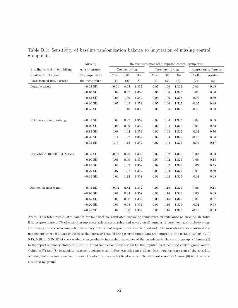
Table B.3: Sensitivity of baseline randomization balance to imputation of missing controlgroup data
Missing Balance statistics with imputed control group data
Baseline covariate exhibiting control group Control group Treatment group Regression difference
treatment imbalance data imputed to Mean SD Obs Mean SD Obs Coeff. p-value
(transformed into z-score) the mean plus: (1) (2) (3) (4) (5) (6) (7) (8)
Durable assets +0.05 SD -0.01 0.95 1,352 0.05 1.06 1,325 0.03 0.49
+0.10 SD 0.02 0.97 1,352 0.05 1.06 1,325 0.01 0.90
+0.15 SD 0.05 1.00 1,352 0.05 1.06 1,325 -0.02 0.69
+0.20 SD 0.07 1.05 1,352 0.05 1.06 1,325 -0.05 0.39
+0.25 SD 0.10 1.10 1,352 0.05 1.06 1,325 -0.08 0.20
Prior vocational training +0.05 SD 0.02 0.97 1,352 0.02 1.04 1,325 0.04 0.39
+0.10 SD 0.05 0.99 1,352 0.02 1.04 1,325 0.01 0.83
+0.15 SD 0.08 1.02 1,352 0.02 1.04 1,325 -0.02 0.70
+0.20 SD 0.11 1.07 1,352 0.02 1.04 1,325 -0.05 0.36
+0.25 SD 0.13 1.12 1,352 0.02 1.04 1,325 -0.07 0.17
Can obtain 100,000 UGX loan +0.05 SD -0.02 0.96 1,352 0.09 1.02 1,325 0.09 0.03
+0.10 SD 0.01 0.99 1,352 0.09 1.02 1,325 0.06 0.15
+0.15 SD 0.04 1.02 1,352 0.09 1.02 1,325 0.03 0.45
+0.20 SD 0.07 1.07 1,352 0.09 1.02 1,325 0.01 0.89
+0.25 SD 0.09 1.12 1,352 0.09 1.02 1,325 -0.02 0.68
Savings in past 6 mo. +0.05 SD -0.02 0.82 1,352 0.06 1.16 1,325 0.06 0.11
+0.10 SD 0.01 0.84 1,352 0.06 1.16 1,325 0.03 0.39
+0.15 SD 0.03 0.88 1,352 0.06 1.16 1,325 0.01 0.87
+0.20 SD 0.06 0.94 1,352 0.06 1.16 1,325 -0.02 0.65
+0.25 SD 0.09 1.00 1,352 0.06 1.16 1,325 -0.05 0.33
Notes: This table recalculates balance for four baseline covariates displaying randomization imbalance at baseline, in Table
B.1. Approximately 6% of control group observations are missing and a very small number of treatment group observations
are missing (people who completed the survey but did not respond to a specific question). All covariates are standardized and
missing treatment data are imputed to the mean, or zero. Missing control group data are imputed to the mean plus 0.05, 0.10,
0.15, 0.20, or 0.25 SD of the variable, thus gradually increasing the values of the covariates in the control group. Columns (1)
to (6) report summary statistics (mean, SD, and number of observations) for the imputed treatment and control group values.
Columns (7) and (8) recalculate treatment-control mean differences using an ordinary least squares regression of the covariate
on assignment to treatment and district (randomization strata) fixed effects. The standard error in Column (8) is robust and
clustered by group.
xi
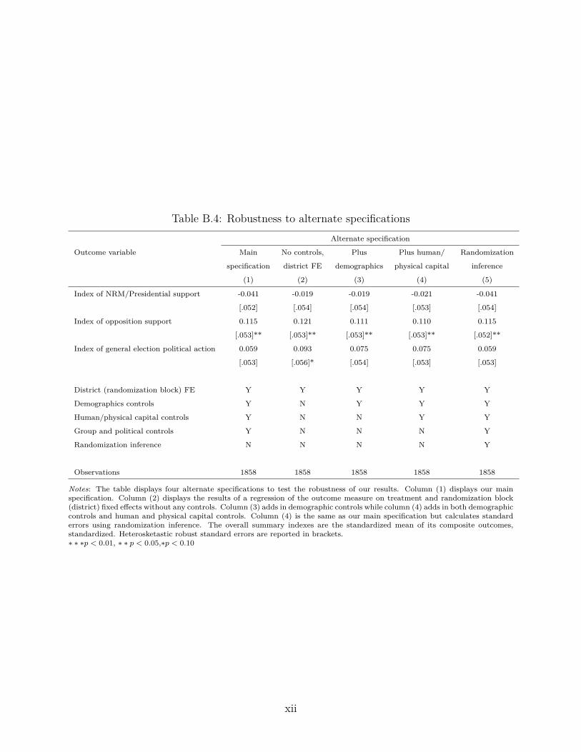
Table B.4: Robustness to alternate specificationsAlternate specification
Outcome variable Main No controls, Plus Plus human/ Randomization
specification district FE demographics physical capital inference
(1) (2) (3) (4) (5)
Index of NRM/Presidential support -0.041 -0.019 -0.019 -0.021 -0.041
[.052] [.054] [.054] [.053] [.054]
Index of opposition support 0.115 0.121 0.111 0.110 0.115
[.053]** [.053]** [.053]** [.053]** [.052]**
Index of general election political action 0.059 0.093 0.075 0.075 0.059
[.053] [.056]* [.054] [.053] [.053]
District (randomization block) FE Y Y Y Y Y
Demographics controls Y N Y Y Y
Human/physical capital controls Y N N Y Y
Group and political controls Y N N N Y
Randomization inference N N N N Y
Observations 1858 1858 1858 1858 1858
Notes: The table displays four alternate specifications to test the robustness of our results. Column (1) displays our mainspecification. Column (2) displays the results of a regression of the outcome measure on treatment and randomization block(district) fixed effects without any controls. Column (3) adds in demographic controls while column (4) adds in both demographiccontrols and human and physical capital controls. Column (4) is the same as our main specification but calculates standarderrors using randomization inference. The overall summary indexes are the standardized mean of its composite outcomes,standardized. Heterosketastic robust standard errors are reported in brackets.∗ ∗ ∗p < 0.01, ∗ ∗ p < 0.05,∗p < 0.10
xii
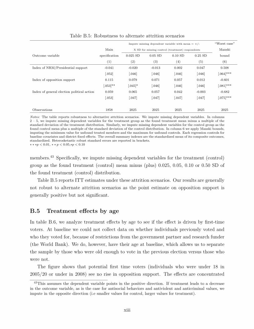
Table B.5: Robustness to alternate attrition scenariosImpute missing dependent variable with mean = +/- “Worst case”
Main X SD for missing control (treatment) respondents Manski
Outcome variable specification 0.025 SD 0.05 SD 0.10 SD 0.25 SD bound
(1) (2) (3) (4) (5) (6)
Index of NRM/Presidential support -0.041 -0.020 -0.013 0.002 0.047 0.508
[.052] [.046] [.046] [.046] [.046] [.064]***
Index of opposition support 0.115 0.079 0.071 0.057 0.012 -0.601
[.053]** [.045]* [.046] [.046] [.046] [.081]***
Index of general election political action 0.059 0.065 0.057 0.042 -0.003 -0.682
[.053] [.047] [.047] [.047] [.047] [.075]***
Observations 1858 2025 2025 2025 2025 2025
Notes: The table reports robustness to alternative attrition scenarios. We impute missing dependent variables. In columns2 – 5, we impute missing dependent variables for the treatment group as the found treatment mean minus a multiple of thestandard deviation of the treatment distribution. Similarly, we impute missing dependent variables for the control group as thefound control mean plus a multiple of the standard deviation of the control distribution. In column 6 we apply Manski bounds,imputing the minimum value for unfound treated members and the maximum for unfound controls. Each regression controls forbaseline covariates and district fixed effects. The overall summary indexes are the standardized mean of its composite outcomes,standardized. Heterosketastic robust standard errors are reported in brackets.∗ ∗ ∗p < 0.01, ∗ ∗ p < 0.05,∗p < 0.10
members.43 Specifically, we impute missing dependent variables for the treatment (control)group as the found treatment (control) mean minus (plus) 0.025, 0.05, 0.10 or 0.50 SD ofthe found treatment (control) distribution.
Table B.5 reports ITT estimates under these attrition scenarios. Our results are generallynot robust to alternate attrition scenarios as the point estimate on opposition support isgenerally positive but not significant.
B.5 Treatment effects by age
In table B.6, we analyze treatment effects by age to see if the effect is driven by first-timevoters. At baseline we could not collect data on whether individuals previously voted andwho they voted for, because of restrictions from the government partner and research funder(the World Bank). We do, however, have their age at baseline, which allows us to separatethe sample by those who were old enough to vote in the previous election versus those whowere not.
The figure shows that potential first time voters (individuals who were under 18 in2005/20 or under in 2008) see no rise in opposition support. The effects are concentrated
43This assumes the dependent variable points in the positive direction. If treatment leads to a decreasein the outcome variable, as is the case for antisocial behaviors and antiviolent and anticriminal values, weimpute in the opposite direction (i.e smaller values for control, larger values for treatment).
xiii

Table B.6: Impacts by ageDV: Opposition support
Effect for
those 20 or
under in
2008
Effect for
those over
20 in 2008
Entire
sample
(1) (2) (3)
Assigned to treatment 0.061 0.142 0.136
[0.090] [0.061]** [0.060]**
Age 20 or under -0.053
[0.071]
Assigned x age 20 or under -0.098
[0.108]
Observations 371 1,487 1858
Notes: The table reports treatment effects on opposition by age as a proxy forfirst time voting. In column 1, we limit the sample to individuals aged 20 or under(or those who were not eligible to vote in the previous election). In column 2, welimit the sample to individuals above the age of 20 (or those eligible to vote intheprevious election). In column 3, we use the entire sample and include a dummyfor being below 20 and an interaction between treatment and the dummy.∗ ∗ ∗p < 0.01, ∗ ∗ p < 0.05,∗p < 0.10
among those who were eligible to vote in the previous election.The lack of impact on young people offers some evidence that the effect we observe is
more about preferences. The impacts are coming from individuals who have more experiencevoting These are not novices with an underdeveloped set of values. They are also more likelyto know the consequences of voting.. However, this is speculative so we take this result withcaution.
B.6 Heterogeneity by fair and random selection
In Table B.7, we display treatment effects by individual’s perceptions of the selection pro-cess. Among those who thought program selection was fair, opposition support rose by 0.13standard deviations, compared to 0.121 standard deviations among those who perceivedselection as unfair. Among those who thought program selection was random, oppositionsupport rose 0.169 standard deviations, compared to 0.123 standard deviations among thosewho perceived selection as non-random
xiv
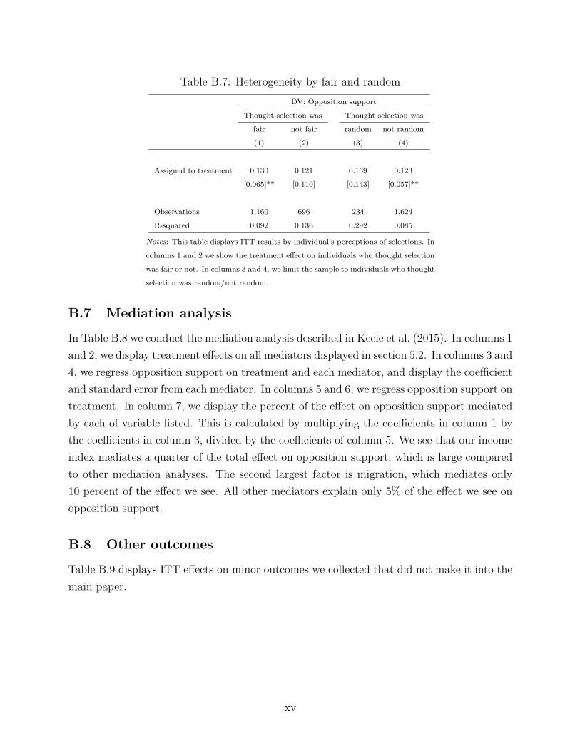
Table B.7: Heterogeneity by fair and randomDV: Opposition support
Thought selection was Thought selection was
fair not fair random not random
(1) (2) (3) (4)
Assigned to treatment 0.130 0.121 0.169 0.123
[0.065]** [0.110] [0.143] [0.057]**
Observations 1,160 696 234 1,624
R-squared 0.092 0.136 0.292 0.085
Notes: This table displays ITT results by individual’s perceptions of selections. In
columns 1 and 2 we show the treatment effect on individuals who thought selection
was fair or not. In columns 3 and 4, we limit the sample to individuals who thought
selection was random/not random.
B.7 Mediation analysis
In Table B.8 we conduct the mediation analysis described in Keele et al. (2015). In columns 1and 2, we display treatment effects on all mediators displayed in section 5.2. In columns 3 and4, we regress opposition support on treatment and each mediator, and display the coefficientand standard error from each mediator. In columns 5 and 6, we regress opposition support ontreatment. In column 7, we display the percent of the effect on opposition support mediatedby each of variable listed. This is calculated by multiplying the coefficients in column 1 bythe coefficients in column 3, divided by the coefficients of column 5. We see that our incomeindex mediates a quarter of the total effect on opposition support, which is large comparedto other mediation analyses. The second largest factor is migration, which mediates only10 percent of the effect we see. All other mediators explain only 5% of the effect we see onopposition support.
B.8 Other outcomes
Table B.9 displays ITT effects on minor outcomes we collected that did not make it into themain paper.
xv

Table B.8: Mediation analysisY: Opposition support; T: Treatment; M: Mediator
Reg. of M on T Reg. of Y on T and M Reg. of Y on T
Coeff. on T Coeff. on M Coeff. on T Percent
Coeff. Std. Err. Coeff. Std. Err. Coeff. Std. Err. mediated
Mediator M (1) (2) (3) (4) (5) (6) (7)
Income, z-score 0.24 [.049]*** 0.12 [.031]*** 0.11 [.053]** 0.25
Index of 2011 election intimidation, z-score 0.04 [.049] 0.12 [.031]*** 0.11 [.053]** 0.04
Existence of a patron, z-score 0.14 [.050]*** -0.01 [.025] 0.11 [.053]** 0.02
Kin relations, z-score 0.05 [.047] -0.05 [.025]* 0.11 [.053]** 0.02
Community participation, z-score 0.00 [.050] 0.01 [.028] 0.11 [.053]** 0
Public goods contributions, z-score 0.01 [.049] -0.01 [.029] 0.11 [.053]** 0
Antisocial behaviors, z-score 0.00 [.047] 0.11 [.033]*** 0.11 [.053]** 0
Protest attitudes and participation, z-score -0.01 [.044] 0.35 [.033]*** 0.11 [.053]** 0.03
Migrated -0.08 [.026]*** 0.17 [.080]** 0.11 [.053]** 0.11
Group cooperation, z-score -0.22 [.128]* -0.02 [.012]** 0.11 [.053]** 0.04
Notes: Columns (1) and (2) represent regressions of each mediator on treatment. Columns (3) and (4) display regressions of
opposition support on treatment and the mediator, Columns (5) and (6) display regressions of opposition support on treatment.
Column (7) displays the percent of the effect of opposition support mediated by the variables listed. This is calculated as the
coefficient in (1) times the coefficient in (2) divided by the coefficient of (3). See Keele et al. (2015) for more details. Standard
errors are heteroskedastic-robust and clustered by group.We calculate the ITT via a weighted least squares regression of the
dependent variable on a program assignment indicator, 13 district (randomization stratum) fixed effects, and a vector of control
variables that includes all of the baseline covariates reported in Appendix B.1.
xvi
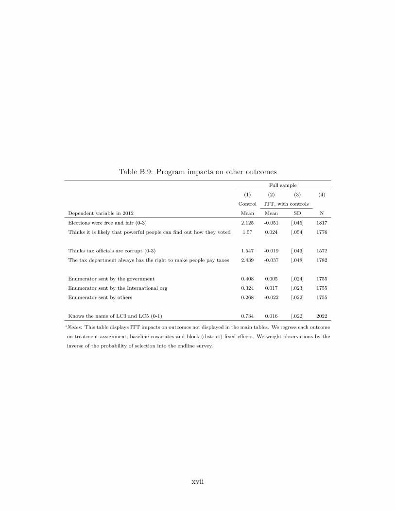
Table B.9: Program impacts on other outcomesFull sample
(1) (2) (3) (4)
Control ITT, with controls
Dependent variable in 2012 Mean Mean SD N
Elections were free and fair (0-3) 2.125 -0.051 [.045] 1817
Thinks it is likely that powerful people can find out how they voted 1.57 0.024 [.054] 1776
Thinks tax officials are corrupt (0-3) 1.547 -0.019 [.043] 1572
The tax department always has the right to make people pay taxes 2.439 -0.037 [.048] 1782
Enumerator sent by the government 0.408 0.005 [.024] 1755
Enumerator sent by the International org 0.324 0.017 [.023] 1755
Enumerator sent by others 0.268 -0.022 [.022] 1755
Knows the name of LC3 and LC5 (0-1) 0.734 0.016 [.022] 2022
‘Notes: This table displays ITT impacts on outcomes not displayed in the main tables. We regress each outcome
on treatment assignment, baseline covariates and block (district) fixed effects. We weight observations by the
inverse of the probability of selection into the endline survey.
xvii


