

EasyMap MAC Protocol
by
Shaoyun Yang
B.Sc., Beijing University of Technology, 2009
Thesis Submitted In Partial Fulfillment of the
Requirements for the Degree of
Master of Applied Science
in the
School of Engineering Science
Faculty of Applied Science
Ó Shaoyun Yang 2013
SIMON FRASER UNIVERSITY
Spring 2013

ii
Approval
Name: Shaoyun Yang
Degree: Master of Applied Science
Title of Thesis: EasyMap MAC Protocol
Examining Committee:
Chair: Dr. Jie Liang Associate Professor, School of Engineering Science
Dr. Daniel C. Lee Senior Supervisor Professor, School of Engineering Science
Dr. Bozena Kaminska Supervisor Professor, School of Engineering Science
Dr. Ash M. Parameswaran Internal Examiner Professor, School of Engineering Science
Date Defended: January 11, 2013

iii
Partial Copyright Licence
iv
Abstract
EasyMap MAC protocol is a new and simple Medium Access Control protocol, which
allows a wireless sensor network to operate with low power and good throughput. This
new protocol is specially designed for the applications which collect data on a relatively
regular schedule and which are required to last for a long period of time. EasyMap
medium access control protocol fits especially well for the wireless networks in which the
wireless sensor nodes are deployed in a linear topology − such as a wireless sensor
network for bridge monitoring, oil pipe monitoring, power distribution system monitoring,
etc.
A special feature of this protocol is that each node transmits relatively short beacon
message of its own in order to announce its presence and to send signalling information
related to the availability timeslots. Such mechanisms address the hidden node problem
and allow the sensor nodes to go to sleep for a large fraction of time and save energy. In
this protocol, nodes are synchronized, and the time line consists of a series of
superframes. Each superframe contains control timeslots and application timeslots. The
relatively shorter length of the control timeslots and the consecutive placement of the
control timeslots in a frame in EasyMap make more application timeslots available for
data transmission or reception.
Keywords: Wireless sensor network; node ID; neighborhood map; duty cycle; slot reservation

v
Acknowledgements
First of all, my sincere thanks to my supervisor Professor Daniel C. Lee for his
strong support during my Master’s. Without his guidance, I could not have found my
research directions and completed the project smoothly. I learnt many significant lessons
from him. Particularly, I learnt to give thoughts before conducting things.
I would like to thank to our research group members, Ehsan Seyedin and Eric
Lee. They gave me lots of great ideas when I was working on this project. Working with
them was a wonderful experience and very productive.
Without the support of my family, I could never have come to Canada and fulfilled
my dream. I also deeply appreciate Corrine and Ying for their support in my daily life and
study.
vi
Table of Contents Approval ..........................................................................................................................ii Partial Copyright Licence ................................................................................................ iii Abstract ..........................................................................................................................iv Acknowledgements......................................................................................................... v Table of Contents............................................................................................................vi List of Tables ..................................................................................................................ix List of Figures ................................................................................................................. x List of Abbreviations.......................................................................................................xii List of Acronyms ........................................................................................................... xiii
1. Introduction .......................................................................................................... 1 1.1.1. IEEE 802.15.4 (LR-WPANs) ....................................................................... 1 1.1.2. Bluetooth Low Energy (BLE)....................................................................... 4
1.2. Existing Wireless Sensor Network Protocols .......................................................... 4 1.3. A Newly Designed MAC Protocol ........................................................................... 6 1.4. Thesis Organization ............................................................................................... 7
2. The Features of EasyMap MAC Protocol............................................................ 8 2.1. Overview................................................................................................................ 8
2.1.1. Logical Topology for EasyMap MAC........................................................... 8 2.1.2. Superframe Structure ................................................................................. 8 2.1.3. MAC Protocol Data Unit (MPDU) ................................................................ 8
2.2. Defining Features................................................................................................... 9 2.2.1. Superframe................................................................................................. 9
Control Section........................................................................................... 9 Beacon Timeslot (BS) ......................................................................... 10 Open-receive-1 timeslot (OR1 timeslot) .............................................. 11 Open-receive-2 timeslot (OR2 timeslot) .............................................. 11
Application Section ................................................................................... 12 Application Timeslots .......................................................................... 12
2.3. Typical Operation................................................................................................. 13
3. Protocol Description in Detail ........................................................................... 16 3.1. Neighborhood Map............................................................................................... 16
3.1.1. Neighborhood Map Overview.................................................................... 16 3.1.2. Neighborhood Map Update Rules............................................................. 18
Rules of Updating in Response to Receiving a Beacon_MPDU (Update Rule 1)................................................................................... 18 Node A Receiving a Beacon_MPDU from a Neighbor that is
neither node A’s parent nor its child (update rule 1.1).................... 18 Node A Receiving from its Parent a Beacon_MPDU (update rule
1.2)................................................................................................ 22 Node A Receiving from its child a Beacon_MPDU (update rule
1.3)................................................................................................ 23 Rules of Updating in Response to Receiving a Non – Beacon_MPDU
(Update Rule 2)................................................................................... 24
vii
Node A Receiving from its parent a Timeslot_Response_MPDU (update rule 2.1)............................................................................ 24
Node A Receiving from its child an ACK_MPDU (update rule 2.2)...................................................................................................... 25
Node A Receiving a Timeslot_Cancellation_MPDU from its child (update rule 2.3)............................................................................ 26
The Rule of Updating after Transmitting a Timeslot_Cancellation_MPDU (Update Rule 3) .................................. 26 Node A Transmitting a Timeslot_Cancellation_MPDU to its
parent (update rule 3.1)................................................................. 26 3.1.3. Spatial Timeslot Reuse............................................................................. 27
3.2. Pre-assignment Formulas and Wakeup Schedule for Control Timeslots .............. 27 3.2.1. Pre-assignment Formulas......................................................................... 28 3.2.2. Wakeup Schedule in Control Section........................................................ 28
3.3. Network Table and Dead Node Detection ............................................................ 30 3.3.1. Network Table (NT) .................................................................................. 30 3.3.2. Dead Node Detection ............................................................................... 31
3.4. Joining Procedure ................................................................................................ 31 3.4.1. Step 1: Scan the Full Superframe............................................................. 31 3.4.2. Step 2: Join the Network........................................................................... 32
3.5. Application Timeslot Negotiation Procedure ......................................................... 32 3.5.1. Proposed timeslots selection .................................................................... 33 3.5.2. Parent validation and response................................................................. 33 3.5.3. Child update and usage............................................................................ 33 3.5.4. Parent update and usage.......................................................................... 34
3.6. Timeslot Reservation Cancellation ....................................................................... 34 3.6.1. Child Cancellation..................................................................................... 34 3.6.2. Parent Cancellation .................................................................................. 35
3.7. Collisions and Resolutions ................................................................................... 36 3.7.1. Collisions .................................................................................................. 36
Collisions in a node’s OR1 timeslot........................................................... 36 Collisions in Reserved Timeslots .............................................................. 38
Reservation Conflict Created by neighboring Nodes that are aware of each other ...................................................................... 40
Reservation Conflict Created by neighboring Nodes that are not fully aware of each other ............................................................... 47
Reservation Conflict Created by neighboring Nodes that are not aware of each other ...................................................................... 52
3.7.2. Resolutions............................................................................................... 54 Carrier Sense ........................................................................................... 54 Exponential Backoff .................................................................................. 55 Resolution for the class-one/class two conflicts、..................................... 55 Periodic Full Control Section Scan............................................................ 55
3.8. Dead Lock and Unlock Process ........................................................................... 57
4. Evaluation........................................................................................................... 60 4.1. Comparison between IEEE 802.15.4 and EasyMap MAC .................................... 60
4.1.1. Performance Metric .................................................................................. 61 4.1.2. Simulation Setup....................................................................................... 62
viii
Simulation Tool and Modules.................................................................... 62 Simulation Configurations......................................................................... 63
4.1.3. Simulation Results and Analysis ............................................................... 67 4.2. Performances Test of EasyMap MAC on a Bridge Health Monitoring
System................................................................................................................. 69 4.2.1. Timeslot Reservation Policy Used ............................................................ 69 4.2.2. Simulation Setup....................................................................................... 70
Simulation Tool and Simulation Module.................................................... 70 Simulation Configurations......................................................................... 71
4.2.3. Performance Metrics................................................................................. 72 Number of Packet Drops and Packet Delivery Ratio................................. 73 Duty Cycle ................................................................................................ 73
4.2.4. Simulation Results and Analysis ............................................................... 74 Number of Dropped Packets..................................................................... 74 Packet Delivery Ratio ............................................................................... 74 Duty Cycle ................................................................................................ 75
5. Conclusion and Future Work............................................................................. 77 5.1. Conclusions ......................................................................................................... 77 5.2. Future Work ......................................................................................................... 78
References .................................................................................................................. 79
Appendices ................................................................................................................. 81 Appendix A. .................................................................................................................. 82 Appendix B. .................................................................................................................. 83
ix
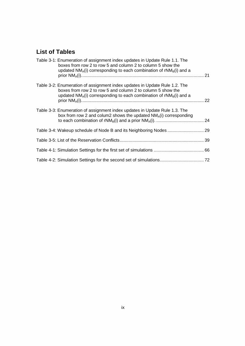
List of Tables Table 3-1: Enumeration of assignment index updates in Update Rule 1.1. The
boxes from row 2 to row 5 and column 2 to column 5 show the updated NMA(i) corresponding to each combination of rNMB(i) and a prior NMA(i).................................................................................................. 21
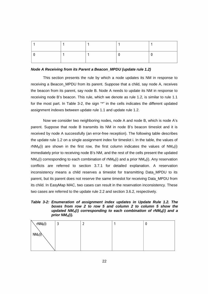
Table 3-2: Enumeration of assignment index updates in Update Rule 1.2. The boxes from row 2 to row 5 and column 2 to column 5 show the updated NMA(i) corresponding to each combination of rNMB(i) and a prior NMA(i).................................................................................................. 22
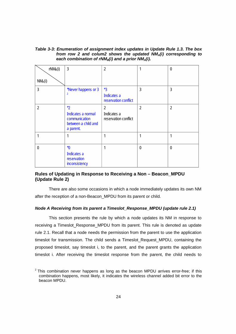
Table 3-3: Enumeration of assignment index updates in Update Rule 1.3. The box from row 2 and colum2 shows the updated NMA(i) corresponding to each combination of rNMB(i) and a prior NMA(i). ...................................... 24
Table 3-4: Wakeup schedule of Node B and its Neighboring Nodes ............................. 29
Table 3-5: List of the Reservation Conflicts ................................................................... 39
Table 4-1: Simulation Settings for the first set of simulations ........................................ 66
Table 4-2: Simulation Settings for the second set of simulations................................... 72
x
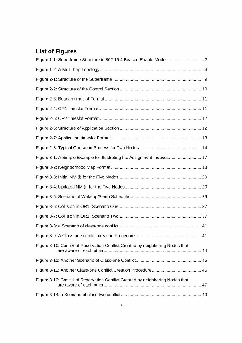
List of Figures Figure 1-1: Superframe Structure in 802.15.4 Beacon Enable Mode .............................. 2
Figure 1-2: A Multi-hop Topology .................................................................................... 4
Figure 2-1: Structure of the Superframe.......................................................................... 9
Figure 2-2: Structure of the Control Section .................................................................. 10
Figure 2-3: Beacon timeslot Format .............................................................................. 11
Figure 2-4: OR1 timeslot Format................................................................................... 11
Figure 2-5: OR2 timeslot Format................................................................................... 12
Figure 2-6: Structure of Application Section .................................................................. 12
Figure 2-7: Application timeslot Format......................................................................... 13
Figure 2-8: Typical Operation Process for Two Nodes .................................................. 14
Figure 3-1: A Simple Example for illustrating the Assignment Indexes.......................... 17
Figure 3-2: Neighborhood Map Format ......................................................................... 18
Figure 3-3: Initial NM (i) for the Five Nodes................................................................... 20
Figure 3-4: Updated NM (i) for the Five Nodes.............................................................. 20
Figure 3-5: Scenario of Wakeup/Sleep Schedule.......................................................... 29
Figure 3-6: Collision in OR1: Scenario One................................................................... 37
Figure 3-7: Collision in OR1: Scenario Two................................................................... 37
Figure 3-8: a Scenario of class-one conflict................................................................... 41
Figure 3-9: A Class-one conflict creation Procedure ..................................................... 41
Figure 3-10: Case 6 of Reservation Conflict Created by neighboring Nodes that are aware of each other............................................................................... 44
Figure 3-11: Another Scenario of Class-one Conflict..................................................... 45
Figure 3-12: Another Class-one Conflict Creation Procedure........................................ 45
Figure 3-13: Case 1 of Reservation Conflict Created by neighboring Nodes that are aware of each other............................................................................... 47
Figure 3-14: a Scenario of class-two conflict ................................................................. 49
xi
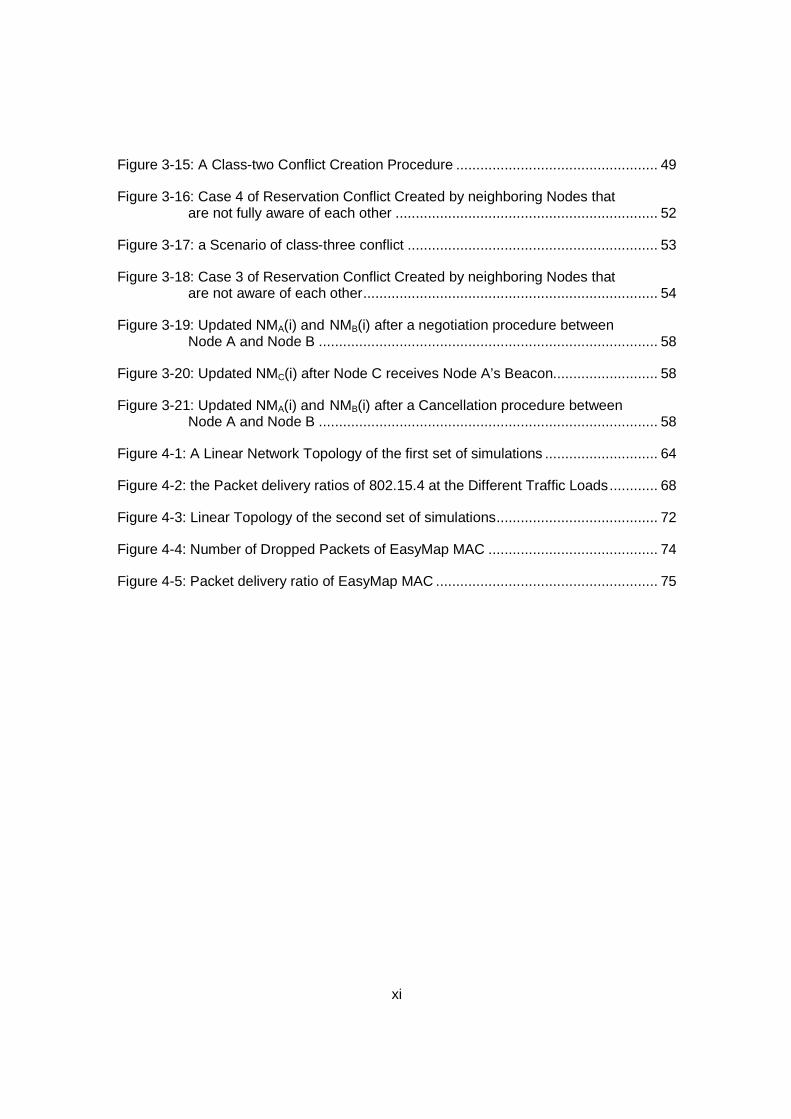
Figure 3-15: A Class-two Conflict Creation Procedure .................................................. 49
Figure 3-16: Case 4 of Reservation Conflict Created by neighboring Nodes that are not fully aware of each other ................................................................. 52
Figure 3-17: a Scenario of class-three conflict .............................................................. 53
Figure 3-18: Case 3 of Reservation Conflict Created by neighboring Nodes that are not aware of each other......................................................................... 54
Figure 3-19: Updated NMA(i) and NMB(i) after a negotiation procedure between Node A and Node B .................................................................................... 58
Figure 3-20: Updated NMC(i) after Node C receives Node A’s Beacon.......................... 58
Figure 3-21: Updated NMA(i) and NMB(i) after a Cancellation procedure between Node A and Node B .................................................................................... 58
Figure 4-1: A Linear Network Topology of the first set of simulations ............................ 64
Figure 4-2: the Packet delivery ratios of 802.15.4 at the Different Traffic Loads............ 68
Figure 4-3: Linear Topology of the second set of simulations........................................ 72
Figure 4-4: Number of Dropped Packets of EasyMap MAC .......................................... 74
Figure 4-5: Packet delivery ratio of EasyMap MAC ....................................................... 75
xii
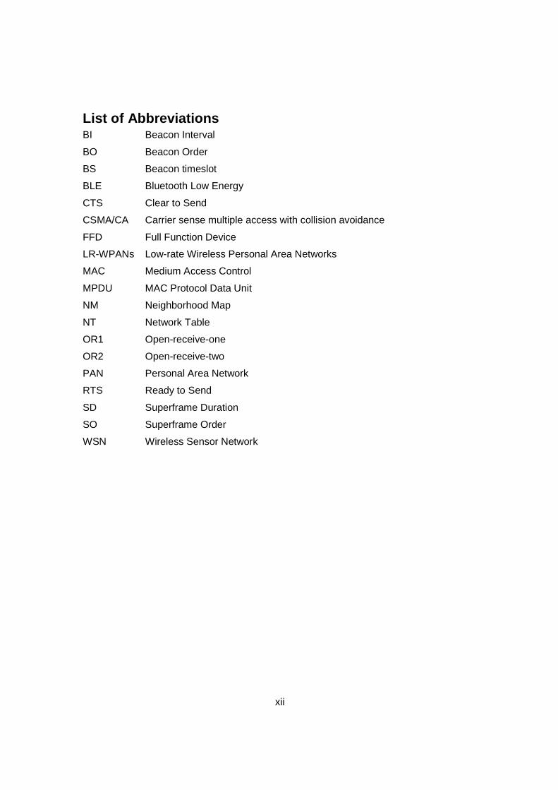
List of Abbreviations BI Beacon Interval
BO Beacon Order
BS Beacon timeslot
BLE Bluetooth Low Energy
CTS Clear to Send
CSMA/CA Carrier sense multiple access with collision avoidance
FFD Full Function Device
LR-WPANs Low-rate Wireless Personal Area Networks
MAC Medium Access Control
MPDU MAC Protocol Data Unit
NM Neighborhood Map
NT Network Table
OR1 Open-receive-one
OR2 Open-receive-two
PAN Personal Area Network
RTS Ready to Send
SD Superframe Duration
SO Superframe Order
WSN Wireless Sensor Network
xiii
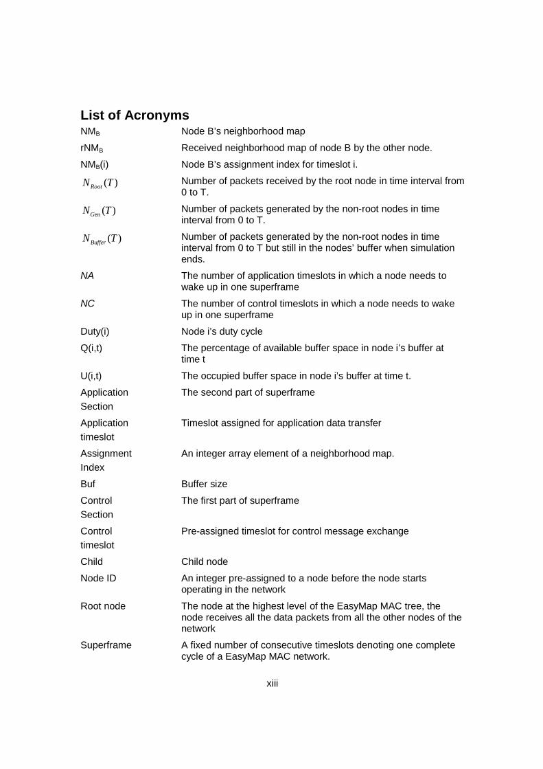
List of Acronyms NMB Node B’s neighborhood map
rNMB Received neighborhood map of node B by the other node.
NMB(i) Node B’s assignment index for timeslot i.
( )RootN T Number of packets received by the root node in time interval from 0 to T.
en ( )GN T Number of packets generated by the non-root nodes in time interval from 0 to T.
( )BufferN T Number of packets generated by the non-root nodes in time interval from 0 to T but still in the nodes’ buffer when simulation ends.
NA The number of application timeslots in which a node needs to wake up in one superframe
NC The number of control timeslots in which a node needs to wake up in one superframe
Duty(i) Node i’s duty cycle
Q(i,t) The percentage of available buffer space in node i’s buffer at time t
U(i,t) The occupied buffer space in node i’s buffer at time t.
Application Section
The second part of superframe
Application timeslot
Timeslot assigned for application data transfer
Assignment Index
An integer array element of a neighborhood map.
Buf Buffer size
Control Section
The first part of superframe
Control timeslot
Pre-assigned timeslot for control message exchange
Child Child node
Node ID An integer pre-assigned to a node before the node starts operating in the network
Root node The node at the highest level of the EasyMap MAC tree, the node receives all the data packets from all the other nodes of the network
Superframe A fixed number of consecutive timeslots denoting one complete cycle of a EasyMap MAC network.

xiv
Tack Transmission time of an acknowledgement
Tg Guard interval between timeslots
1
1. Introduction
In this chapter, we introduce two low-energy wireless standards, IEEE 802.15.4
and Bluetooth low energy, and present the disadvantages when those protocols are
used for wireless sensor networks. We also present other current MAC protocols that
can be used for wireless sensor networks and their features. Then, this chapter
introduces features of EasyMap MAC protocol which has been developed at Simon
Fraser University and is the main topic of this thesis. Then we describe the organization
of rest of the thesis.
1.1.1. IEEE 802.15.4 (LR-WPANs)
IEEE 802.15.4 [1] is a standard which specifies the physical layer and media
access control for low-rate wireless personal area networks (LR-WPANs). It is
maintained by the IEEE 802.15.4 working group. The IEEE 802.15.4 standard also
specifies the currently most significant commercially adopted MAC protocol for wireless
sensor networks [2].
The IEEE 802.15.4 MAC provides two modes of operation, the asynchronous
beaconless and the synchronous beacon enabled mode. The beaconless mode requires
nodes to listen for other nodes’ transmission all the time, which can drain battery power
fast. The beacon enabled mode is designed to support the transmission of beacon
packets between transmitter and receiver providing synchronization among nodes.
Synchronization allows devices to sleep between coordinated transmissions, which
results in energy efficiency and prolonged network lifetimes.
In IEEE 802.15.4, the device that can broadcast beacon is called Full Function
Device (FFD), can act as a router in multi-hop topologies. On the other hand, the device
that cannot broadcast beacon is called Reduced Function Device (RFD), can only
operate as the end device. In the beacon enabled mode, devices synchronize their
2
actions and coordinate data transmission with each other. FFDs periodically transmit
beacons to synchronize wakeup/sleep schedules with the neighboring nodes. Channel
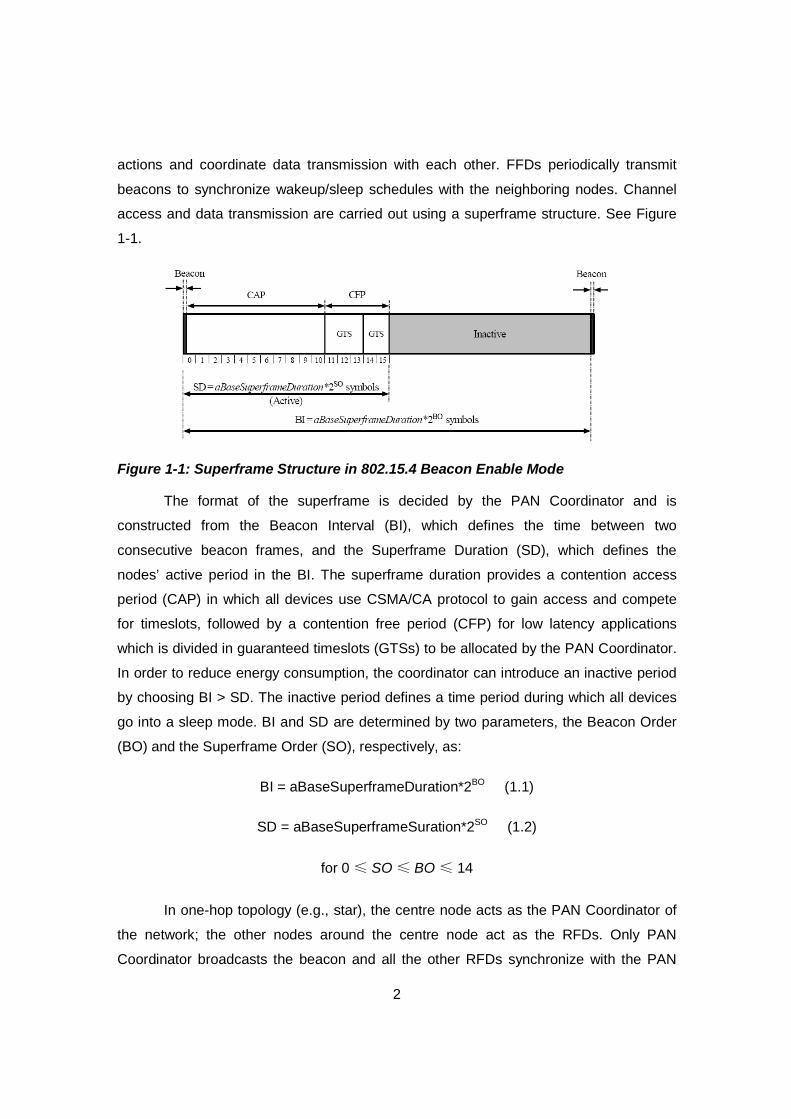
access and data transmission are carried out using a superframe structure. See Figure
1-1.
Figure 1-1: Superframe Structure in 802.15.4 Beacon Enable Mode
The format of the superframe is decided by the PAN Coordinator and is
constructed from the Beacon Interval (BI), which defines the time between two
consecutive beacon frames, and the Superframe Duration (SD), which defines the
nodes’ active period in the BI. The superframe duration provides a contention access
period (CAP) in which all devices use CSMA/CA protocol to gain access and compete
for timeslots, followed by a contention free period (CFP) for low latency applications
which is divided in guaranteed timeslots (GTSs) to be allocated by the PAN Coordinator.
In order to reduce energy consumption, the coordinator can introduce an inactive period
by choosing BI > SD. The inactive period defines a time period during which all devices
go into a sleep mode. BI and SD are determined by two parameters, the Beacon Order
(BO) and the Superframe Order (SO), respectively, as:
BI = aBaseSuperframeDuration*2BO (1.1)
SD = aBaseSuperframeSuration*2SO (1.2)
for 0 ≤ SO ≤ BO ≤ 14
In one-hop topology (e.g., star), the centre node acts as the PAN Coordinator of
the network; the other nodes around the centre node act as the RFDs. Only PAN
Coordinator broadcasts the beacon and all the other RFDs synchronize with the PAN
3
Coordinator. All the devices, PAN Coordinator included, have the same wake up/sleep
schedule. The communication between a device and the PAN Coordinator only occurs in
the active period.
IEEE 802.15.4, indeed, can achieve very low energy consumption, which meets
the basic requirement of wireless sensor networks. However, the disadvantages of IEEE
802.15.4 are also obvious. Firstly, IEEE 802.15.4 with beacon enabled mode does not
define when a FFD broadcasts its own beacon in multi-hop topologies [3], and thus IEEE
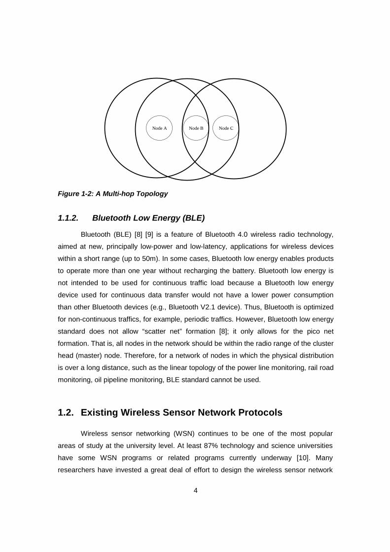
802.15.4 does not work for multi-hop topologies. Figure 1-2 shows a simple multi-hop
topology. Suppose node A is the Pan Coordinator, node B is a FFD, and node B is node
A’s child. Since IEEE 802.15.4 does not define that when node B broadcasts its beacon,
node C cannot join the network. The multi-hop topology cannot be formed in IEEE
802.15.4. Thus, IEEE 802.15.4 is not intended to work for multi-hop topologies.
Secondly, IEEE 802.15.4 does not solve hidden node problem at all [4], and thus the
network efficiency cannot be guaranteed because of the collisions. Specifically, IEEE
802.15.4 standard only defines one type of CSMA/CA (the Physical Carrier Sense in
802.11), and the RTS/CTS mechanism is not used in IEEE 802.15.4. Thus the hidden
node problem can decrease the performance of IEEE 802.15.4. Last but not the least,
the CSMA/CA algorithm defined in IEEE 802.15.4 does not perform quite well, especially
in the heavy traffic loads. The network is not reliable when the traffic load is heavy [5].
Although IEEE 802.15 works better with the modified CSMA/CA algorithm [6] [7],
CSMA/CA of IEEE 802.15.4 introduces some overhead to the network. Nodes waste
some wakeup time in performing the CSMA/CA. Thus, the wakeup time is not efficiently
used by nodes, which can decrease the throughput of an IEEE 802.15.4 network.
4
`
Node A
Node B
Node C
Figure 1-2: A Multi-hop Topology
1.1.2. Bluetooth Low Energy (BLE)
Bluetooth (BLE) [8] [9] is a feature of Bluetooth 4.0 wireless radio technology,
aimed at new, principally low-power and low-latency, applications for wireless devices
within a short range (up to 50m). In some cases, Bluetooth low energy enables products
to operate more than one year without recharging the battery. Bluetooth low energy is
not intended to be used for continuous traffic load because a Bluetooth low energy
device used for continuous data transfer would not have a lower power consumption
than other Bluetooth devices (e.g., Bluetooth V2.1 device). Thus, Bluetooth is optimized
for non-continuous traffics, for example, periodic traffics. However, Bluetooth low energy
standard does not allow “scatter net” formation [8]; it only allows for the pico net
formation. That is, all nodes in the network should be within the radio range of the cluster
head (master) node. Therefore, for a network of nodes in which the physical distribution
is over a long distance, such as the linear topology of the power line monitoring, rail road
monitoring, oil pipeline monitoring, BLE standard cannot be used.
1.2. Existing Wireless Sensor Network Protocols
Wireless sensor networking (WSN) continues to be one of the most popular
areas of study at the university level. At least 87% technology and science universities
have some WSN programs or related programs currently underway [10]. Many
researchers have invested a great deal of effort to design the wireless sensor network
5
protocols. S-MAC [11] is an early-age WSN protocol. The main goal of S-MAC protocol
design is to reduce energy consumption, while supporting good scalability and collision
avoidance. S-MAC protocol divides the time into frames whose length is determined by
applications. There are work period and sleep period in a frame. S-MAC adopts an
effective mechanism (namely, periodical listening and sleep) to solve the energy wasting
problems. Each node goes to sleep for some time, and then wakes up and listens to see
if any other node wants to talk to it. The listen/sleep mechanism reduces the wasting of
energy; however, the predefined and constant sleep and listen periods decrease the
efficiency of the algorithm under variable traffic load [12].
T-MAC [12] is an improvement to S-MAC to reduce energy consumption on idle
listening. It introduces an adaptive duty cycle: all messages are transmitted in variable
length bursts and the lengths of bursts are dynamically determined. Similar to S-MAC,
T-MAC has active periods and sleep periods in a time frame. An active period ends if
there is no activity for a particular time period, which we denote as Ta. Ta is the minimum
listening time in the time frame. T-MAC reduces the time in the active state, compared
with S-MAC, but it suffers from early sleeping problem – node goes to sleep when a
neighbor still has messages for it.
A new WSN protocol, the Powermesh MAC protocol [13] released in 2011, is a
relatively simple protocol designed for sensor network applications such as monitoring of
a power distribution system. The neighborhood map is the core idea of the protocol to
solve the hidden node problem and to achieve low duty cycle. Specifically, the
neighborhood map, which is a defining feature of the Powermesh MAC protocol, is a
small data structure that indicates timeslot usage of the node’s neighbors’. By using the
neighborhood map, each node is able to negotiate efficiently with its parent regarding
the available timeslots for data transmission. The probability of the packets collision is
greatly reduced by using the neighborhood map. The nodes only talk to each other in
the timeslots specifically reserved through the negotiation; the nodes are able to sleep
for the most of time of a superframe. Thus, the low duty cycle is another advantage of
the Powermesh MAC protocol.
The NapMap MAC protocol [14] is an improvement of the Powermesh MAC
protocol. In the NapMap MAC protocol, a node needs to receive all the neighbors’

6
beacon packets rather than just the parent’s and the child’s, which enables the node to
have better perception of its neighborhoods and thus reduce the number of collisions.
Secondly, the NapMap MAC protocol changed the indications of the assignment indexes.
The new assignment indexes work more efficiently when updating the neighborhood
map. Allowing multiple transactions in a single application time is also an improvement
of the Powermesh MAC protocol.
There are also some other WSN protocols have been proposed in the past years,
and those protocols are really hybrid, such as Z-MAC [15], B-MAC [16], etc.
1.3. A Newly Designed MAC Protocol
We designed a new WSN protocol, which we named EasyMap MAC protocol.
The protocol’s basic objective is to work for the small or medium wireless sensor
networks with low duty cycle and high-reliability performance (e.g., high packet delivery
ratio). EasyMap MAC protocol solves problems with hidden nodes by using two new
methods: node ID pre-assignment and neighborhood map (NM). The new methods
guarantee the nodes work with high packet delivery ratio and low duty cycle.
Unlike the Powermesh MAC and Napmap MAC protocol, a single superframe
consists of two sections, and the two-section superframe format allows the collision-free
transmission/reception in the control timeslots. The uniqueness of each control timeslot
of each node successfully eliminates the control timeslot collisions. The shorter length of
the control timeslot decreases the overhead of the control timeslots and thus reduces
the duty cycle. The simplicity is another advantage of the EasyMap MAC protocol.
Due to the fixed control timeslots pre-assignment mechanism in EasyMap MAC
protocol, the number of nodes in one wireless network system is limited. As a result, the
limitation constrains the wireless network scale. The protocol would work best with small
or medium wireless networks and is not intended to work for the large wireless network
systems.

7
The set-up processes, which include the joining part and negotiation part, are
very time-consuming, sometimes requiring several minutes. As a result, EasyMap MAC
protocol is not intended to work for real-time wireless sensor networks. EasyMap MAC
protocol works optimally for a wireless network that can endure some end-to-end delay.
1.4. Thesis Organization
The thesis is organized as follows. The features of the EasyMap MAC protocol
are reviewed in Chapter 2. In Chapter 3, we present the core ideas of the EasyMap MAC
protocol. Especially, we discuss the two crucial methods, node ID and neighborhood
map. In Chapter 4, we use Network Simulator 2 (NS-2) to present the simulation results
for EasyMap MAC protocol and IEEE 802.15.4. We also test the performances of
EasyMap MAC for a particular application; namely, a bridge health monitoring system. In
the end, we present the future work and conclude the thesis in Chapter 5. Some other
definitions used in this thesis are listed in Appendices.

8
2. The Features of EasyMap MAC Protocol
2.1. Overview
2.1.1. Logical Topology for EasyMap MAC
The EasyMap MAC protocol supports one logical topology: tree topology. In the
tree topology, the child sends data to the parent. The parent forwards those data, along
with its own, to its parent and eventually the data are delivered to the root node.
2.1.2. Superframe Structure
The EasyMap MAC protocol uses a time-slot structure. A single superframe is
divided into 518 timeslots. Once a superframe finishes, the next superframe follows
immediately.
2.1.3. MAC Protocol Data Unit (MPDU)
Each node can transmit four different types of MPDUs in the network. Those are
Beacon_MPDU, Data_MPDU, ACK_MPDU, and Control_Message_MPDUs. The Contr-
ol_Message_MPDUs consist of Association_Request_MPDU, Association_Response_-
MPDU, Timeslot_Request_MPDU, Timeslot_Response_MPDU, and Timeslots_Cancell-
ation_MPDU. The Data_MPDU and Control_Message_MPDUs require an ACK_MPDU
from the receiving node back to the sending node.
9
2.2. Defining Features
2.2.1. Superframe
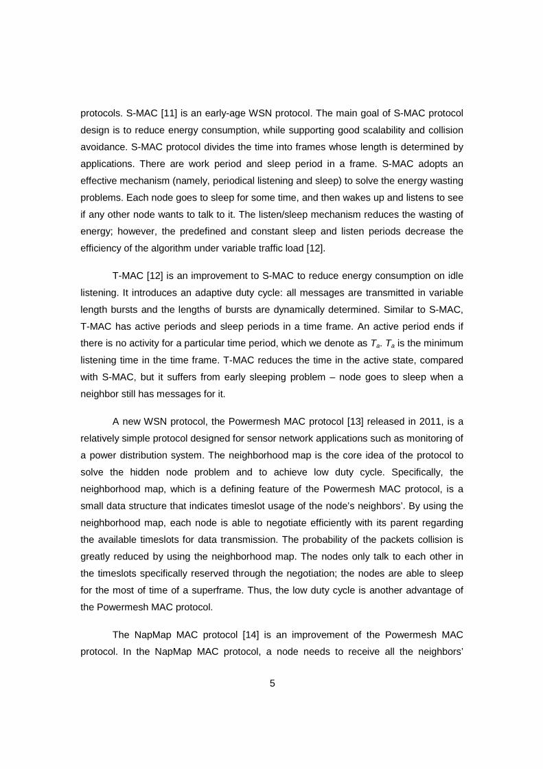
Figure 2-1 shows the structure of superframe. The superframe length is 8
seconds. In EasyMap MAC protocol, a superframe consists of two different sections:
control section (1 second) and application section (7 seconds). The control section is in
the first part of superframe and application section is in the second part of superframe.
Figure 2-1: Structure of the Superframe
Control Section
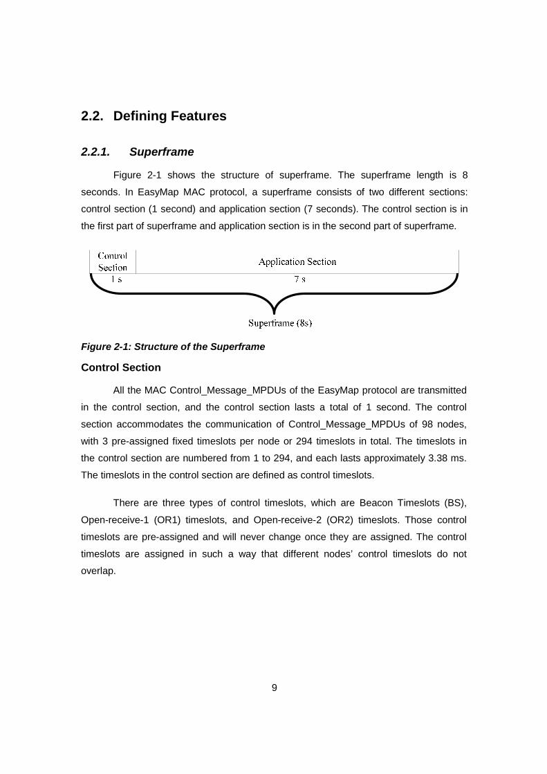
All the MAC Control_Message_MPDUs of the EasyMap protocol are transmitted
in the control section, and the control section lasts a total of 1 second. The control
section accommodates the communication of Control_Message_MPDUs of 98 nodes,
with 3 pre-assigned fixed timeslots per node or 294 timeslots in total. The timeslots in
the control section are numbered from 1 to 294, and each lasts approximately 3.38 ms.
The timeslots in the control section are defined as control timeslots.
There are three types of control timeslots, which are Beacon Timeslots (BS),
Open-receive-1 (OR1) timeslots, and Open-receive-2 (OR2) timeslots. Those control
timeslots are pre-assigned and will never change once they are assigned. The control
timeslots are assigned in such a way that different nodes’ control timeslots do not
overlap.
10
ControlSection
1 2 3 4 294 293……
(1s)
3.38ms
Figure 2-2: Structure of the Control Section
Each node in the system would be pre-assigned with three control timeslots: (i)
BS, (ii) OR1 timeslot and (iii) OR2 timeslot, before the node starts to operate in the
network. Each node performs different kinds of actions in different control timeslots. As
long as the control timeslots are pre-assigned to a node, other nodes cannot use those
pre-assigned timeslots. In other words, the control timeslots in control section are not
even spatially reusable in this protocol. For example, if timeslots 1, 2 and 3 are pre-
assigned to node 0, these three control timeslots belong to node 0 until node 0 stops
operating in the network.
Beacon Timeslot (BS)
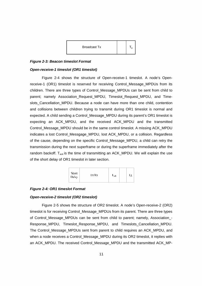
Figure 2-3 shows the format of beacon timeslot. A node transmits its
Beacon_MPDU in its beacon timeslot. The Beacon_MPDU is a node’s primary method
of announcing its presence to other nodes. Since the beacon is a broadcast message,
no ACK_MPDU is expected. Each node is required to transmit its beacon once per
superframe. Because of hardware differences, clock synchronization is not exact.
Differences in timekeeping can cause nodes to have small differences in the boundaries
of timeslots. To compensate for these differences, EasyMap MAC protocol defines a
fixed guard interval, denoted Tg. If a node is scheduled to listen or receive a packet in
timeslot i, then the node must begin listening Tg before the beginning of timeslot i.
Similarly, any transmissions in a timeslot must be completed Tg before the end of that
timeslot.
11
Figure 2-3: Beacon timeslot Format
Open-receive-1 timeslot (OR1 timeslot)
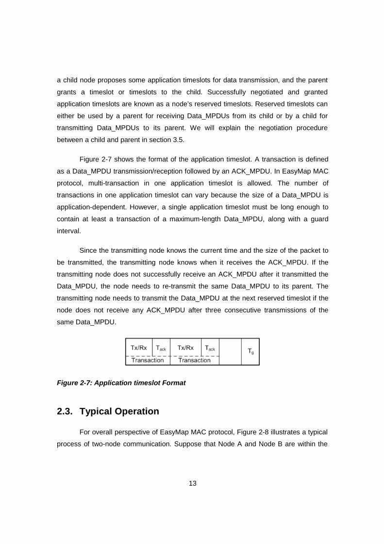
Figure 2-4 shows the structure of Open-receive-1 timeslot. A node’s Open-
receive-1 (OR1) timeslot is reserved for receiving Control_Message_MPDUs from its
children. There are three types of Control_Message_MPDUs can be sent from child to
parent; namely Association_Request_MPDU, Timeslot_Request_MPDU, and Time-
slots_Cancellation_MPDU. Because a node can have more than one child, contention
and collisions between children trying to transmit during OR1 timeslot is normal and
expected. A child sending a Control_Message_MPDU during its parent’s OR1 timeslot is
expecting an ACK_MPDU, and the received ACK_MPDU and the transmitted
Control_Message_MPDU should be in the same control timeslot. A missing ACK_MPDU
indicates a lost Control_Messgage_MPDU, lost ACK_MPDU, or a collision. Regardless
of the cause, depending on the specific Control_Message_MPDU, a child can retry the
transmission during the next superframe or during the superframe immediately after the
random backoff. Tack is the time of transmitting an ACK_MPDU. We will explain the use
of the short delay of OR1 timeslot in later section.
Figure 2-4: OR1 timeslot Format
Open-receive-2 timeslot (OR2 timeslot)
Figure 2-5 shows the structure of OR2 timeslot. A node’s Open-receive-2 (OR2)
timeslot is for receiving Control_Message_MPDUs from its parent. There are three types
of Control_Message_MPDUs can be sent from child to parent; namely, Association_-
Response_MPDU, Timeslot_Response_MPDU, and Timeslots_Cancellation_MPDU.
The Control_Message_MPDUs sent from parent to child requires an ACK_MPDU, and
when a node receives a Control_Message_MPDU during its OR2 timeslot, it replies with
an ACK_MPDU. The received Control_Message_MPDU and the transmitted ACK_MP-

12
DU should be in the same control timeslot. Because each node has only one parent,
collisions and contention are not expected during the node’s OR2 timeslot. Because the
root node does not have parent, it does not have OR2 timeslot. Except the root node, all
the other nodes are required to be awake during their OR2 timeslots.
Figure 2-5: OR2 timeslot Format
Application Section
All application data transmission will take place during the application section.
The length of an application section is 7 seconds. There are 224 timeslots (each 31.25
ms long) in the application section, and the timeslots are numbered from 295 to 518,
following the consecutive numbering of the control section. The 518th timeslot is the final
timeslot of the superframe. The timeslots in the application section are referred to
application timeslots.
Figure 2-6: Structure of Application Section
Application Timeslots
The application timeslots for a node are used for transmitting Data_MPDUs to its
parent or receiving Data_MPDUs from its child. A node needs the permission from its
parent if the node wants to reserve the application timeslot for transmitting data packets
to its parent. Otherwise the node cannot use the application timeslot for transmission. If
a node wants to reserve an application timeslot, it needs to perform a negotiation
process, and the negotiation is authorized by its parent. During the negotiation process,
13
a child node proposes some application timeslots for data transmission, and the parent
grants a timeslot or timeslots to the child. Successfully negotiated and granted
application timeslots are known as a node’s reserved timeslots. Reserved timeslots can
either be used by a parent for receiving Data_MPDUs from its child or by a child for
transmitting Data_MPDUs to its parent. We will explain the negotiation procedure
between a child and parent in section 3.5.
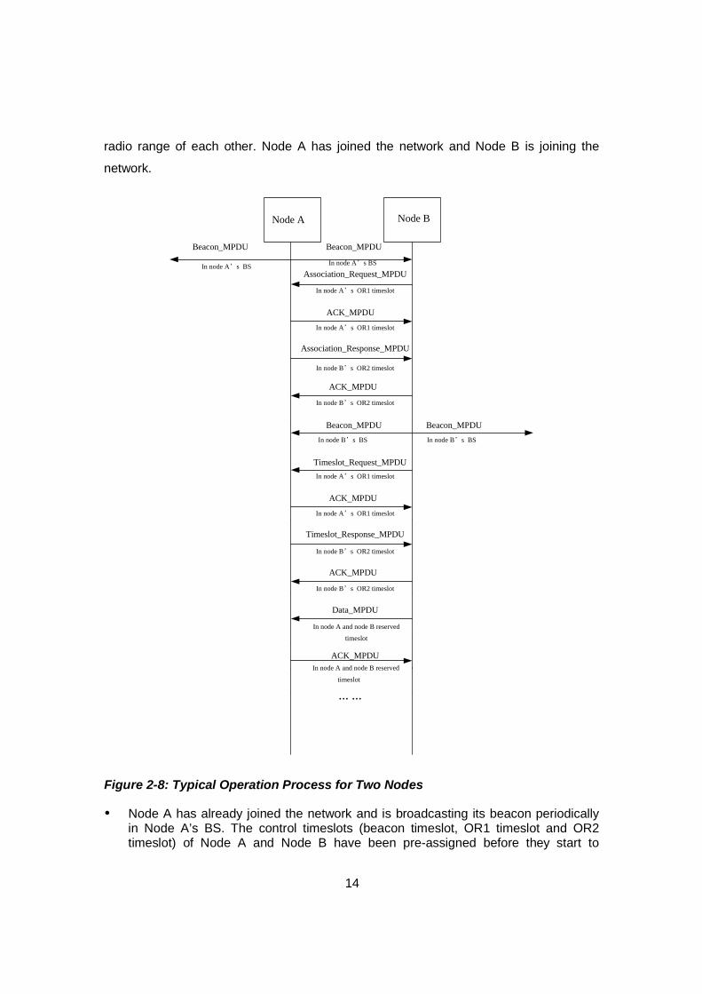
Figure 2-7 shows the format of the application timeslot. A transaction is defined
as a Data_MPDU transmission/reception followed by an ACK_MPDU. In EasyMap MAC
protocol, multi-transaction in one application timeslot is allowed. The number of
transactions in one application timeslot can vary because the size of a Data_MPDU is
application-dependent. However, a single application timeslot must be long enough to
contain at least a transaction of a maximum-length Data_MPDU, along with a guard
interval.
Since the transmitting node knows the current time and the size of the packet to
be transmitted, the transmitting node knows when it receives the ACK_MPDU. If the
transmitting node does not successfully receive an ACK_MPDU after it transmitted the
Data_MPDU, the node needs to re-transmit the same Data_MPDU to its parent. The
transmitting node needs to transmit the Data_MPDU at the next reserved timeslot if the
node does not receive any ACK_MPDU after three consecutive transmissions of the
same Data_MPDU.
Figure 2-7: Application timeslot Format
2.3. Typical Operation
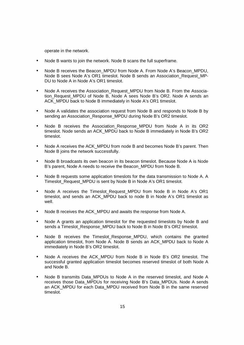
For overall perspective of EasyMap MAC protocol, Figure 2-8 illustrates a typical
process of two-node communication. Suppose that Node A and Node B are within the
14
radio range of each other. Node A has joined the network and Node B is joining the
network.
Node A Node B
Association_Request_MPDU
In node A’s OR1 timeslot
ACK_MPDU
In node B’s OR2 timeslot
Beacon_MPDU
In node A’s BSIn node A’s BS
Data_MPDU
In node A and node B reserved
timeslot
In node A and node B reserved
timeslot
… …
Beacon_MPDU
In node A’s OR1 timeslot
Association_Response_MPDU
ACK_MPDU
In node B’s OR2 timeslot
Beacon_MPDU
In node B’s BS
Beacon_MPDU
In node B’s BS
Timeslot_Request_MPDU
In node A’s OR1 timeslot
ACK_MPDU
In node A’s OR1 timeslot
Timeslot_Response_MPDU
In node B’s OR2 timeslot
ACK_MPDU
In node B’s OR2 timeslot
ACK_MPDU
Figure 2-8: Typical Operation Process for Two Nodes
Ÿ Node A has already joined the network and is broadcasting its beacon periodically in Node A’s BS. The control timeslots (beacon timeslot, OR1 timeslot and OR2 timeslot) of Node A and Node B have been pre-assigned before they start to
15
operate in the network.
Ÿ Node B wants to join the network. Node B scans the full superframe.
Ÿ Node B receives the Beacon_MPDU from Node A. From Node A’s Beacon_MPDU, Node B sees Node A’s OR1 timeslot. Node B sends an Association_Request_MP-DU to Node A in Node A’s OR1 timeslot.
Ÿ Node A receives the Association_Request_MPDU from Node B. From the Associa-tion_Request_MPDU of Node B, Node A sees Node B’s OR2. Node A sends an ACK_MPDU back to Node B immediately in Node A’s OR1 timeslot.
Ÿ Node A validates the association request from Node B and responds to Node B by sending an Association_Response_MPDU during Node B’s OR2 timeslot.
Ÿ Node B receives the Association_Response_MPDU from Node A in its OR2 timeslot. Node sends an ACK_MPDU back to Node B immediately in Node B’s OR2 timeslot.
Ÿ Node A receives the ACK_MPDU from node B and becomes Node B’s parent. Then Node B joins the network successfully.
Ÿ Node B broadcasts its own beacon in its beacon timeslot. Because Node A is Node B’s parent, Node A needs to receive the Beacon_MPDU from Node B.
Ÿ Node B requests some application timeslots for the data transmission to Node A. A Timeslot_Request_MPDU is sent by Node B in Node A’s OR1 timeslot.
Ÿ Node A receives the Timeslot_Request_MPDU from Node B in Node A’s OR1 timeslot, and sends an ACK_MPDU back to node B in Node A’s OR1 timeslot as well.
Ÿ Node B receives the ACK_MPDU and awaits the response from Node A.
Ÿ Node A grants an application timeslot for the requested timeslots by Node B and sends a Timeslot_Response_MPDU back to Node B in Node B’s OR2 timeslot.
Ÿ Node B receives the Timeslot_Response_MPDU, which contains the granted application timeslot, from Node A. Node B sends an ACK_MPDU back to Node A immediately in Node B’s OR2 timeslot.
Ÿ Node A receives the ACK_MPDU from Node B in Node B’s OR2 timeslot. The successful granted application timeslot becomes reserved timeslot of both Node A and Node B.
Ÿ Node B transmits Data_MPDUs to Node A in the reserved timeslot, and Node A receives those Data_MPDUs for receiving Node B’s Data_MPDUs. Node A sends an ACK_MPDU for each Data_MPDU received from Node B in the same reserved timeslot.
16
3. Protocol Description in Detail
3.1. Neighborhood Map
3.1.1. Neighborhood Map Overview
The neighborhood map (NM) describes a node’s current perception of
application timeslot assignments in its neighborhood. If a node (either joined the network
or not) can hear a Beacon_MPDU from another node, these two nodes are neighbors of
each other although they do not have parent-child relation. Basically, the nodes are
neighbors if the nodes are within the radio range of each other.
The neighborhood map (NM) is an array of integers, with one integer
corresponding to each timeslot in the application section. The index has four values, 3
(11), 2 (10), 1 (01) and 0 (00). All the indexes of neighborhood map should be initialized
to 0 before a node starts to operate in networks. A notation NMA represents the NM of
node A. That is, node A’s neighborhood map is denoted by NMA. NMA(i) represents the
value of timeslot i of node A’s neighborhood map. Those indexes in the NM are called
assignment indexes. Each assignment index value has a different meaning in EasyMap
MAC protocol. The node updates its own neighborhood map by changing those
assignment indexes. Figure 3-1 shows a scenario for illustrating the assignment indexes.

17
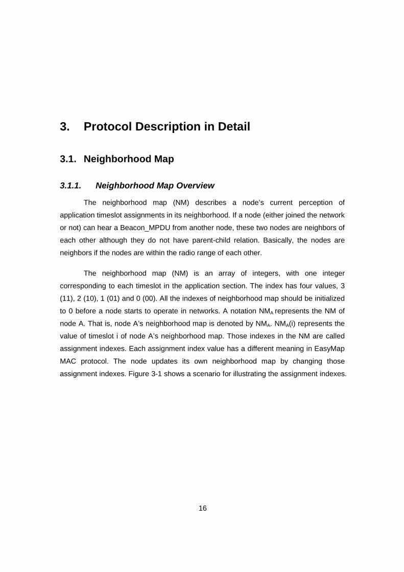
Figure 3-1: A Simple Example for illustrating the Assignment Indexes
Assignment index = 3: NMA(i) = 3 indicates that timeslot i is being used as node
A’s own reserved timeslot for transmitting Data_MPDUs to its parent.
Assignment index = 2: NMA(i) = 2 indicates that timeslot i is being used as node
A’s own reserved timeslot for receiving Data_MPDU from its child.
Assignment index = 1: NMA(i) = 1 indicates that timeslot i is being used by one
of Node A’s neighbors, say node B, as node B’s reserved timeslot for receiving or
transmitting Data_MPDUs. Specifically, at timeslot i, node A cannot communicate with
any node in its neighborhood. This is because the communication between node A and
any node in node A’s neighborhood would cause a collision with node B. Thus, node A
can neither propose timeslot i nor grant timeslot i.
Assignment index = 0: NMA(i) = 0 indicates that none of Node A’s neighbors
has been assigned with timeslot i as a reserved timeslot, and hence Node A can either
propose timeslot i or grant timeslot i.
The neighborhood map field is in the Beacon_MPDU, and it accounts for 56
Bytes. Figure 3-2 shows the format of neighborhood map.

18
Figure 3-2: Neighborhood Map Format
3.1.2. Neighborhood Map Update Rules
In EasyMap MAC, timeslot assignment is dynamic, and as such, the
neighborhood map (NM) must be updated and maintained to reflect the changing
timeslot assignments of its neighbors’. Each node is required to store and update its own
neighborhood map. During normal network operations, a node updates its neighborhood
map according to different update rules.、
Rules of Updating in Response to Receiving a Beacon_MPDU (Update Rule 1)
Each node keeps its own neighborhood map, and the neighborhood map guides
the node when and what to do in each application timeslot. Recall that a node, say node
B, wakes up and transmits Data_MPDU to its parent (e.g., node A) if the assignment
index of a timeslot i is 3 in its NM. Node B wakes up and receives Data_MPDU from its
child (e.g., node C) if the assignment index of a timeslot i is 2 in its NM. The node
receives its neighbors’ Beacon_MPDUs periodically. A node can receive the
Beacon_MPDU from three types of neighbor, which are the node’s neighbors, but they
don’t have parent-child relation, the node’s parent, and the node’s child. Thus, three
types of update rules in response to receiving a Beacon_MPDU are defined.
Node A Receiving a Beacon_MPDU from a Neighbor that is neither node A’s parent nor its child (update rule 1.1)
This section presents the rule by which a node updates its NM in response to
receiving a Beacon_MPDU from a neighbor that is neither the node’s parent nor its child.
This rule is denoted as rule 1.1. Suppose node A and node B are neighbors but not in
parent-child relation. NMA and NMB represent the neighborhood map of node A and
node B, respectively. Now, node A is receiving node B’s Beacon_MPDU. Node B’s
neighborhood map that another node (e.g., node A) receives is denoted to rNMB. If a
node (e.g., node A) successfully receives node B’s NMA (an error-free reception),
19
rNMB = NMB (3.1)
Upon receiving the neighborhood map from node B, each assignment index in
the neighborhood map of node A should be updated as the following:
NMA(i) : = max [ t (rNMB (i)), NMA (i) ], i = 295, 296,...,517, 518 (3.2)
where the function t( ) is defined as t(3) = 1, t(2) = 1, t(1) = 0, t(0) = 0.
The updated neighborhood map NMA consists of the updated assignment
indexes (NMA (i), i = 295, 296,…,517, 518).
All the assignment indexes of all the application timeslots should be updated
according to neighborhood update rule 1.1. To explain the neighborhood map update
rule 1.1 more clearly, the following example illustrates the assignment index update
process for a specific timeslot i. The following paragraphs illustrate the procedure of the
assignment index update process. Also see the scenario in Figure 3-3 and Figure 3-4.
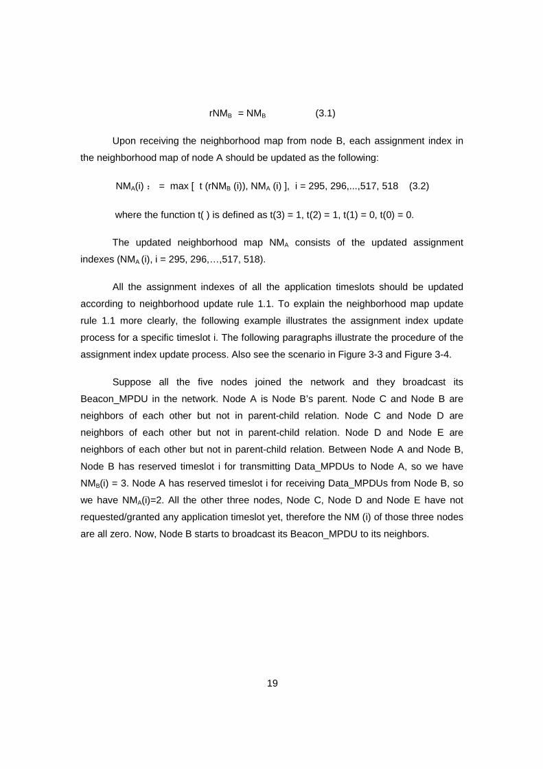
Suppose all the five nodes joined the network and they broadcast its
Beacon_MPDU in the network. Node A is Node B’s parent. Node C and Node B are
neighbors of each other but not in parent-child relation. Node C and Node D are
neighbors of each other but not in parent-child relation. Node D and Node E are
neighbors of each other but not in parent-child relation. Between Node A and Node B,
Node B has reserved timeslot i for transmitting Data_MPDUs to Node A, so we have
NMB(i) = 3. Node A has reserved timeslot i for receiving Data_MPDUs from Node B, so
we have NMA(i)=2. All the other three nodes, Node C, Node D and Node E have not
requested/granted any application timeslot yet, therefore the NM (i) of those three nodes
are all zero. Now, Node B starts to broadcast its Beacon_MPDU to its neighbors.
20
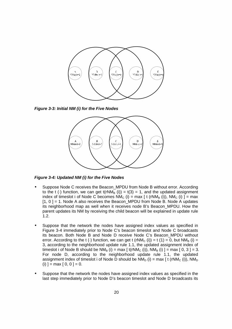
Figure 3-3: Initial NM (i) for the Five Nodes
Figure 3-4: Updated NM (i) for the Five Nodes
Ÿ Suppose Node C receives the Beacon_MPDU from Node B without error. According to the t (·) function, we can get t(rNMB (i)) = t(3) = 1, and the updated assignment index of timeslot i of Node C becomes NMC (i) = max [ t (rNMB (i)), NMC (i) ] = max [1, 0 ] = 1. Node A also receives the Beacon_MPDU from Node B. Node A updates its neighborhood map as well when it receives node B’s Beacon_MPDU. How the parent updates its NM by receiving the child beacon will be explained in update rule 1.2.
Ÿ Suppose that the network the nodes have assigned index values as specified in Figure 3-4 immediately prior to Node C’s beacon timeslot and Node C broadcasts its beacon. Both Node B and Node D receive Node C’s Beacon_MPDU without error. According to the t (·) function, we can get t (rNMC (i)) = t (1) = 0, but NMB (i) = 3, according to the neighborhood update rule 1.1, the updated assignment index of timeslot i of Node B should be NMB (i) = max [ t(rNMC (i)), NMB (i) ] = max [ 0, 3 ] = 3. For node D, according to the neighborhood update rule 1.1, the updated assignment index of timeslot i of Node D should be NMD (i) = max [ t (rNMC (i)), NMD (i) ] = max [ 0, 0 ] = 0.
Ÿ Suppose that the network the nodes have assigned index values as specified in the last step immediately prior to Node D’s beacon timeslot and Node D broadcasts its
21
beacon. Both Node C and Node E receive the Beacon_MPDU from Node D without error. According to the t (·) function, we can get t (rNMD (i)) = t (0) = 0, but NMC(i) = 1; according to the neighborhood update rule 1.1, the updated assignment index of timeslot i of node C should be NMC (i) = max [ t (rNMD (i)), NMC (i) ] = max [ 0, 1 ] = 1. On the other hand, for Node E, according to the neighborhood update rules 1.1, the updated assignment index of timeslot i of Node E should be NME (i) = max [ t (rNMD (i)), NME (i) ] = max [ 0, 0 ] = 0.
Figure 3-4 shows the final updated NM (i) of the five nodes.
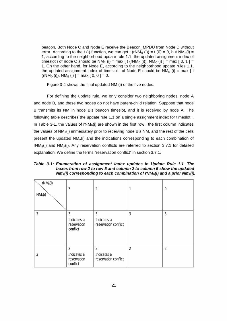
For defining the update rule, we only consider two neighboring nodes, node A
and node B, and these two nodes do not have parent-child relation. Suppose that node
B transmits its NM in node B’s beacon timeslot, and it is received by node A. The
following table describes the update rule 1.1 on a single assignment index for timeslot i.
In Table 3-1, the values of rNMB(i) are shown in the first row , the first column indicates
the values of NMA(i) immediately prior to receiving node B’s NM, and the rest of the cells
present the updated NMA(i) and the indications corresponding to each combination of
rNMB(i) and NMA(i). Any reservation conflicts are referred to section 3.7.1 for detailed
explanation. We define the terms “reservation conflict” in section 3.7.1.
Table 3-1: Enumeration of assignment index updates in Update Rule 1.1. The boxes from row 2 to row 5 and column 2 to column 5 show the updated NMA(i) corresponding to each combination of rNMB(i) and a prior NMA(i).
rNMB(i) NMA(i)
3
2
1
0
3 3 Indicates a reservation conflict
3 Indicates a reservation conflict
3 3
2
2 Indicates a reservation conflict
2 Indicates a reservation conflict
2 2
22
1 1 1 1 1
0 1 1 0 0
Node A Receiving from its Parent a Beacon_MPDU (update rule 1.2)
This section presents the rule by which a node updates its NM in response to
receiving a Beacon_MPDU from its parent. Suppose that a child, say node A, receives
the beacon from its parent, say node B. Node A needs to update its NM in response to
receiving node B’s beacon. This rule, which we denote as rule 1.2, is similar to rule 1.1
for the most part. In Table 3-2, the sign “*” in the cells indicates the different updated
assignment indexes between update rule 1.1 and update rule 1.2.
Now we consider two neighboring nodes, node A and node B, which is node A’s
parent. Suppose that node B transmits its NM in node B’s beacon timeslot and it is
received by node A successfully (an error-free reception). The following table describes
the update rule 1.2 on a single assignment index for timeslot i. In the table, the values of
rNMB(i) are shown in the first row, the first column indicates the values of NMA(i)
immediately prior to receiving node B’s NM, and the rest of the cells present the updated
NMA(i) corresponding to each combination of rNMB(i) and a prior NMA(i). Any reservation
conflicts are referred to section 3.7.1 for detailed explanation. A reservation
inconsistency means a child reserves a timeslot for transmitting Data_MPDU to its
parent, but its parent does not reserve the same timeslot for receiving Data_MPDU from
its child. In EasyMap MAC, two cases can result in the reservation inconsistency. These
two cases are referred to the update rule 2.2 and section 3.6.2, respectively.
Table 3-2: Enumeration of assignment index updates in Update Rule 1.2. The boxes from row 2 to row 5 and column 2 to column 5 show the updated NMA(i) corresponding to each combination of rNMB(i) and a prior NMA(i).
rNMB(i) NMA(i)
3 2 1 0

23
3 *Never happens if rNMB(i) is received error free. 3 1
*3 Indicates a normal communication between a child and a parent.
*0 Indicates a reservation inconsistency
*0 Indicates a reservation inconsistency
2 2 Indicates a reservation conflict
2 Indicates a reservation conflict
2 2
1 1 1 1 1
0 1 1 0 0
Node A Receiving from its child a Beacon_MPDU (update rule 1.3)
This section presents the rule by which a node updates its NM in response to
receiving a Beacon_MPDU from its child. Suppose that a parent, say node A, receives a
beacon from its child, say node B. Node A needs to update its NM in response to
receiving node B’s beacon. Table 3-3 presents this update rule. This rule, which we
denote as rule 1.3, is similar to rule 1.1 for the most part. In Table 3-3, the sign “*” in the
cells indicates the different updated assignment indexes between update rule 1.1 and
update rule 1.3.
For defining the update rule, we consider two neighboring nodes, node A and
node B. In this illustration, node B is node A’s child. Suppose that node B transmits its
NM in node B’s beacon timeslot, and it is received by node A successfully (an error-free
reception). Table 3-3 describes rule 1.3 on a single assignment index for timeslot i. In
the table, the values of rNMB(i) are shown in the first row. The first column indicates the
values of NMA(i) immediately prior to receiving node B’s NM. The rest of the cells
present the updated NMA(i) and the also what is indicated by the combination of rNMB(i)
and a prior NMA(i). Any reservation conflicts and are referred to section 3.7.1 for detailed
explanation 1 This combination never happens as long as the beacon MPDU arrives error-free; if this
combination happens, most likely, it indicates the wireless channel added bit error to the beacon MPDU.
24
Table 3-3: Enumeration of assignment index updates in Update Rule 1.3. The box from row 2 and colum2 shows the updated NMA(i) corresponding to each combination of rNMB(i) and a prior NMA(i).
rNMB(i) NMA(i)
3 2 1 0
3 *Never happens or 3 2
*3 Indicates a reservation conflict
3 3
2 *2 Indicates a normal communication between a child and a parent.
2 Indicates a reservation conflict
2 2
1 1 1 1 1
0 *0 Indicates a reservation inconsistency
1 0 0
Rules of Updating in Response to Receiving a Non – Beacon_MPDU (Update Rule 2)
There are also some occasions in which a node immediately updates its own NM
after the reception of a non-Beacon_MPDU from its parent or child.
Node A Receiving from its parent a Timeslot_Response_MPDU (update rule 2.1)
This section presents the rule by which a node updates its NM in response to
receiving a Timeslot_Response_MPDU from its parent. This rule is denoted as update
rule 2.1. Recall that a node needs the permission from the parent to use the application
timeslot for transmission. The child sends a Timeslot_Request_MPDU, containing the
proposed timeslot, say timeslot i, to the parent, and the parent grants the application
timeslot i. After receiving the timeslot response from the parent, the child needs to
2 This combination never happens as long as the beacon MPDU arrives error-free; if this
combination happens, most likely, it indicates the wireless channel added bit error to the beacon MPDU.
25
update its neighborhood map. The updated assignment index of the newly granted
timeslot for the child should be set to 3 in its own NM. Suppose a child, say node A,
already sent a Timeslot_Request_MPDU, containing the proposed timeslot, say timeslot
i, to its parent, say node B. Node B grants timeslot i to node A, and node B sends a
Timeslot_Response_MPDU to node A. Node A updates its neighborhood map
immediately in response to receiving the Timeslot_Response_MPDU, which contains
the granted timeslot i, from node B. Finally, NMA (i) = 0 is updated to NMA (i) = 3.
Node A Receiving from its child an ACK_MPDU (update rule 2.2)
This section presents the rule by which a node updates its neighborhood map in
response to receiving an ACK_MPDU from its child after it sent a Timeslot_Response_-
MPDU to its child. This rule is denoted as update rule 2.2. A parent updates its own NM
in response to receiving an ACK_MPDU from its child if it sent a Timeslot_Respon-
se_MPDU to its child before receiving the ACK_MPDU. Specifically, a parent, say node
A, does not update its neighborhood map right after sending the Timeslot_Respon-
se_MPDU, which contains the information of the granted application timeslot, say
timeslot i, to its child, say node B. This is because node A wants to make sure that node
B successfully receives the Timeslot_Response_MPDU and reserves the granted
timeslot i by receiving the ACK_MPDU from node B. Node A would assume that node B
does not receive the Timeslot_Response_MPDU, and node B does not reserve timeslot
i if node A does not receive an ACK_MPDU from node B after it sent a Timeslot_Res-
ponse_MPDU to node B. However, if node A receives the ACK_MPDU from node B,
node A updates its own NM. The updated assignment index of the newly granted
timeslot i of node A should be set to 2 in node A’s own NM. Node A will use timeslot i for
receiving Data_MPDU from node B.
However, update rule 2.2 can create the reservation inconsistency between a
parent and child when the ACK_MPDU is lost. Specifically, if a child node, say node A,
successfully receives the Timeslot_Response_MPDU from its parent, say node B, and
node A updates its NM by changing the assignment index of the newly granted timeslot,
say timeslot i. Node A needs to send an ACK_MPDU back to node B. But sometimes
the ACK_MPDU can be lost due to some reasons (e.g., low-quality link), and thus node
B cannot receive the ACK_MPDU from node A. Node B will not update its NM, and NMB
26
(i) = 0 because node B assumes node A does not receive the Timeslot_Respon-
se_MPDU. Thus, NMA (i) = 3 and NMB (i) = 0 creates the reservation inconsistence
between node A and node B, which results in the packets loss at timeslot i because
node A is transmitting Data_MPDU to node B but node B is sleeping. To stop
transmitting packets in timeslot i, node A must notice the reservation inconsistency
problem, and stop transmitting Data_MPDU to node B as quickly as possible. According
to the update rule 1.2, node A can easily detect the reservation inconsistency because
NMA (i) = 3 and NMB (i) = 0. Node B needs to cancel timeslot i itself by changing the
assignment index of timeslot i from NMA (i) = 3 to NMA (i) = 0, and thus the problem is
resolved. For the parent, node B does not need to update its NM because node A can
fix the problem by itself.
Node A Receiving a Timeslot_Cancellation_MPDU from its child (update rule 2.3)
This section presents the rule by which a parent updates its neighborhood map in
response to receiving a Timeslot_Cancellation_MPDU from its child. This rule is denoted
as update rule 2.3. Suppose a node, say nod A, needs to immediately update its
neighborhood map in response to receiving a Timeslot_Cancellation_MPDU from its
child, say node B. The updated assignment index of the cancelled timeslot, say timeslot i,
should be set to 0 in node A’s neighborhood map. When node A receives a
Timeslot_Cancellation_MPDU from node B, node A should update its neighborhood map
immediately by changing the assignment index of timeslot i from NMA (i) = 2 to NMA (i) =
0.
The Rule of Updating after Transmitting a Timeslot_Cancellation_MPDU (Update Rule 3)
Node A Transmitting a Timeslot_Cancellation_MPDU to its parent (update rule 3.1)
This section presents the rule by which a child updates its NM after transmitting
a Timeslot_Cancellation_MPDU to its parent. This rule is denoted as update rule 3.1.
Suppose a node, say node A, needs to immediately update its neighborhood map after
transmitting a Timeslot_Cancellation_MPDU to its parent, say node B. The updated
assignment index of the cancelled timeslot, say timeslot i, should be set to 0 in node A’s
neighborhood map after transmitting a Timeslot_Cancellation_MPDU to node B. Node A

27
should update its neighborhood map immediately by changing the assignment index of
timeslot i from NMA (i) = 3 to NMA (i) = 0.
3.1.3. Spatial Timeslot Reuse
Recall that neighborhood map presents the availability of the application
timeslots, and also allows the spatial timeslots reuse. As indicated by the assignment
index definitions (as described in section 3.1.1), the application timeslot is available to a
node for reservation if that application timeslot has assignment index of 0 in the node’s
own NM. If an application timeslot, say timeslot i, has be assigned to a node either for
transmission or reception, the assignment index of timeslot i of the node must be greater
than 1. To let the application timeslots be spatially reusable, the function t(·) in the
update rules is designed so that the assignment index can be 0 for a node farther apart
from a node to which the timeslot is assigned. Therefore, the application timeslot can
also be assigned to the other nodes.
Figure 3-4 provides an illustration. Timeslot i has been reserved by Node A and
Node B for their reception and transmission, respectively. According to the definitions of
the assignment indexes, timeslot i is reusable for Node D and Node E because NMD (i) =
0 and NME (i) = 0. Thus, the application timeslots can be spatially re-used by nodes.
3.2. Pre-assignment Formulas and Wakeup Schedule for Control Timeslots
Each node will be pre-assigned a node ID before it operates in the network. The
node ID determines a node’s control timeslots according to the formula = to be explained
in section 3.2.1. A node receives its neighbors’ node IDs from the Beacon_MPDUs, but
a node can also see its neighbors’ node IDs from other MPDUs (e.g., Association_Re-
quest_MPDU).
28
3.2.1. Pre-assignment Formulas
Given that the pre-assigned node ID to each node, the control timeslots of each
node are pre-assigned. Unlike the application timeslots, control timeslots are not
spatially reusable. In other words, each node has its three unique control timeslots.
The pre-assigned control timeslots can be, for example, in accordance with the
following formulas.
B.S (Beacon timeslot) = 3 * n + 1; (3.3)
OR1 (Open – receive 1) timeslot = 3 * n + 2; (3.4)
OR2 (Open – receive 2) timeslot = 3 * n + 3; (3.5)
Where n is the node ID and the node ID can be 0, 1, … , 97
For example, before operating in the network, a node A has been pre-assigned a
node ID 20. According to the pre-assignment formulas (3.3) to (3.5), node A’s BS, OR1
timeslot, and OR2 timeslot are slot 61, 62, and 63, respectively.
3.2.2. Wakeup Schedule in Control Section
A node wakes up and sleeps in the application section according to its
neighborhood map. In the control section, the node wakes up and sleeps according to
its own node ID and the node IDs of its neighbors. A node, say node B, needs to scan
the full superframe to receive all the Beacon_MPDUs (including neighbors’ NMs and
node IDs) from its neighbors when it is joining the network. According to the pre-
assignment formulas (3.3) to (3.5), node B not only wakes up in its own control timeslots
(node B’s BS, OR1 timeslot, and OR2 timeslot), it also optionally wakes up in their
neighbors’ control timeslots. For example, node B wakes up in its parent’s BS and OR1
timeslot, but it sleeps in its parent’s OR2 timeslot.
If a node, say node B, has joined the network. Node has its parent, child, and a
neighbor which does not have parent-child relation with node B. Node B needs to wake
up in certain control timeslots to communicate with all its neighbors. The following table
29
and paragraph show the wakeup schedule of node B and its neighbors in the control
section.
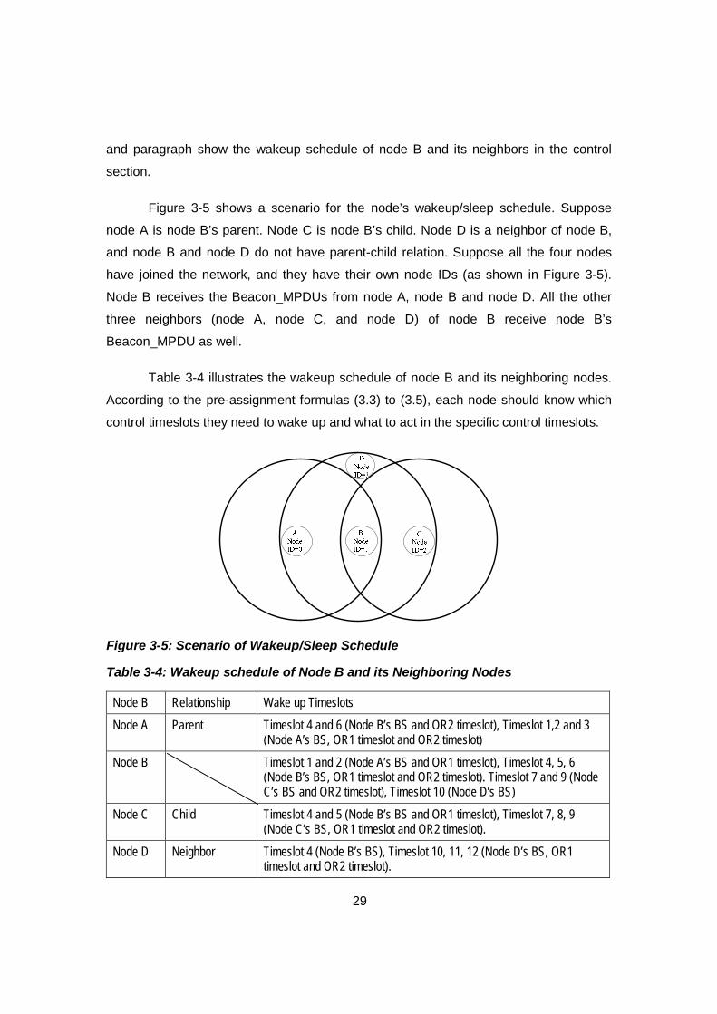
Figure 3-5 shows a scenario for the node’s wakeup/sleep schedule. Suppose
node A is node B’s parent. Node C is node B’s child. Node D is a neighbor of node B,
and node B and node D do not have parent-child relation. Suppose all the four nodes
have joined the network, and they have their own node IDs (as shown in Figure 3-5).
Node B receives the Beacon_MPDUs from node A, node B and node D. All the other
three neighbors (node A, node C, and node D) of node B receive node B’s
Beacon_MPDU as well.
Table 3-4 illustrates the wakeup schedule of node B and its neighboring nodes.
According to the pre-assignment formulas (3.3) to (3.5), each node should know which
control timeslots they need to wake up and what to act in the specific control timeslots.
Figure 3-5: Scenario of Wakeup/Sleep Schedule
Table 3-4: Wakeup schedule of Node B and its Neighboring Nodes
Node B Relationship Wake up Timeslots
Node A Parent Timeslot 4 and 6 (Node B’s BS and OR2 timeslot), Timeslot 1,2 and 3 (Node A’s BS, OR1 timeslot and OR2 timeslot)
Node B Timeslot 1 and 2 (Node A’s BS and OR1 timeslot), Timeslot 4, 5, 6 (Node B’s BS, OR1 timeslot and OR2 timeslot). Timeslot 7 and 9 (Node C’s BS and OR2 timeslot), Timeslot 10 (Node D’s BS)
Node C Child Timeslot 4 and 5 (Node B’s BS and OR1 timeslot), Timeslot 7, 8, 9 (Node C’s BS, OR1 timeslot and OR2 timeslot).
Node D Neighbor Timeslot 4 (Node B’s BS), Timeslot 10, 11, 12 (Node D’s BS, OR1 timeslot and OR2 timeslot).

30
Ÿ Node B and Node A: Because node A is node B’s parent, node B needs to wake up at node A’ beacon timeslot (timeslot 1) to receive node A’s beacon. Node B sends its request MPDU (e.g., Timeslot_Request_MPDU) at node A’s OR1 timeslot (timeslot 2). Node A needs to wake up at node B’s beacon timeslot (timeslot 4) to receive node B’s beacon. Node A sends the response (e.g., Timeslot_Respon-se_MPDU) back to node B in node B’s OR2 timeslot (timeslot 6).
Ÿ Node B and Node C: Because node C is node B’ child, node B needs to wake up to receive node C’s beacon at node C’s beacon timeslot (timeslot 7) and send the response MPDU (e.g., Timeslot_Response_MPDU) to node C at node C’s OR2 timeslot (timeslot 9). Node C needs to wake up to receive node B’s beacon at node B’s BS timeslot (timeslot 4) and send the request MPDU (e.g., Timeslot_Re-quest_MPDU) to node B at node B’s OR1 timeslot (timeslot 5).
Ÿ Node B and Node D: Because node D and node B do not have parent-child relation. Node B needs to wake up to receive node D’s Beacon_MPDU at node D’s beacon timeslot (timeslot 10). Node D needs to wake up to receive node B’s Beacon_MP-DU at node B’s BS timeslot (timeslot 4).
3.3. Network Table and Dead Node Detection
3.3.1. Network Table (NT)
Recall that only up to 98 nodes can work in the system, and even a smaller
number of nodes will be working in the network if some nodes die. The dead nodes
cannot conduct normal communication in the network due to specific reasons such as
the expired battery or RF problems. As a result, the data supposed to be collected by
the root node cannot be sensed by the dead nodes, and thus some information would
be lost due to the dead nodes. The dead nodes have to be detected as quickly as
possible. In EasyMap MAC protocol, network table is introduced to help detect the dead
nodes in the network.
The Network table (NT) is an array of integers, with one integer
corresponding to each node’s node ID, and there are up to 98 integers (from 0 to 97,
corresponding to 98 nodes) in the NT. The indexes of those integers in the NT are called
pre-assignment indexes. All the pre-assignment indexes are initialized to 0 before the
first node is installed to the network. Recall that each node would be assigned with a
node ID before operating in the network. The pre-assignment index of the node ID

31
should update to 1 in the NT once the node ID has been assigned to a node. For
example, a node ID with a value 4 has been assigned to a node. The third integer in the
NT should be updated to 1, which means node ID 4 has been assigned to a node. Only
the root node keeps the network table. According the network table, the health of the
nodes in the network can be presented.
3.3.2. Dead Node Detection
The network table helps the dead node detection in the network. The payload of
a Data_MPDU may contain the node ID of the source node. Ideally, the root node is
supposed to receive all the Data_MPDUs from all the other nodes in the network. Hence,
a node would be detected to be dead if the root node does not receive any Data_MPDU
from a node (e.g., node B) for a long time (e.g., one hour). The nodes with pre-
assignment indexes of 1 in NT are detected to be dead if the root node does not receive
any Data_MPDUs from those nodes for a long time. If a dead node has been detected,
the installers can either fix the problem of that dead node and keep the pre-assignment
index 1 of that node in the network table, or just release the node ID of the dead node
and set the pre-assignment index to 0 in the network table.
3.4. Joining Procedure
3.4.1. Step 1: Scan the Full Superframe
When a node B wants to join the EasyMap network, it initializes its NM to all
zeros, and then performs at least one superframe length scan. During the full
superframe scan, node B receives all its neighbors’ beacons, which contain the
neighbors’ NMs and node IDs. Node B updates its NMB whenever node B receives a
Beacon_MPDU from one of its neighbors according to the NM update rule 1.1. In
addition, when a new neighbor is first discovered by receiving the new neighbor’s arrival
beacon, node B needs to record its new neighbor’s node ID. This is because node B
needs to wake up at the certain control timeslots of its neighbors.

32
One of the node B’s neighbors becomes the parent of node B after a full
superframe scan. There are different policies by which a joining node chooses its parent.
A proposed policy called first-beacon policy illustrates how node B chooses its parent. In
the scanning process, the joining node receives all the Beacon_MPDUs from its
neighbors. However, the joining node only chooses one of its neighbors to be its parent.
If a joining node, say node B, receives the first Beacon_MPDU from a node (e.g., node
A), node B will choose node A as its parent.
3.4.2. Step 2: Join the Network
After the scan process, node B needs to send an Association_Request_MPDU to
its parent, say node A, at node A’s OR1 timeslot. Node B awaits an ACK_MPDU from
node A. Node A receives the Association_Request_MPDU from node B, sees node B’s
node ID from the Association_Request_MPDU, and sends an ACK_MPDU back to node
B immediately at its OR1 timeslot. Node B might need to rejoin node A if node B does
not receive an ACK_MPDU after it sends the Association_Request_MPDU to Node A.
Otherwise node B awaits a reply at its OR2 timeslot. During node B’s OR2 timeslot,
node A should make a decision if node B can be its child. Node A sends a negative reply
if node A denies node B’s association request or a positive reply if node B can be its
child. Node B becomes node A’s child after node A sends a positive reply to node B at
node B’ OR2 timeslot. If node B receives the positive reply from node A, it sends an
ACK_MPDU back to node A immediately at its OR2 timeslot. Node B has to join the
other node (e.g., node G) if node B receives a negative reply from node A. After node B
sends the ACK_MPDU back to node A, node B assumes the joining process succeed
and starts to broadcast its Beacon_MPDU at its BS timeslot since the next superframe.
Node A receives the ACK_MPDU from node B at node B’s OR2 timeslot and needs to
listen to node B’s Beacon_MPDU at node B’s BS timeslot since the next superframe.
3.5. Application Timeslot Negotiation Procedure
After a node joins the network, in order to transmit Data_MPDUs to its parent,
the node should request application timeslots from its parent for transmission. The
nodes propose available timeslots to its parent. The proposed application timeslots must

33
have an assignment index of 0 in the node’s own neighborhood map. Before an
application timeslot can be used, permission must be granted by the parent.
3.5.1. Proposed timeslots selection
If a node, say node B wants to transmit data to its parent, it must request an
application timeslot or application timeslots for data transmission. Firstly, node B should
check its own NMB to identify the timeslots with assignment indexes of 0, and select
some number of proposed timeslots. For example, a node, say node B sends the
Timeslot_Request_MPDU, which contains the information of which application timeslots
are being proposed, to its parent, say node A, at the parent’s (node A’s) OR1 timeslot,
and awaits an ACK_MPDU from node A. Upon receiving node B’s
Timeslot_Request_MPDU, node A sends an ACK_MPDU back to node B at node A’s
OR1 timeslot. Node B receives the ACK_MPDU from node A at node A’s OR1, and
awaits for node A’s response at node B’s OR2 timeslot. If node B does not receive an
ACK_MPDU from node A after it sends the request message, node B has to request the
timeslot again during the next superframe or during the superframe immediately after
the random backoff.
3.5.2. Parent validation and response
Upon receiving the Timeslot_Request_MPDU from node B, node A compares
the proposed timeslots with its own NMA and select only the timeslots whose
assignment index is 0 in node A’s NM. Among these timeslots, node A decides which
timeslots to grant to node B. Node A can grant any or none of the proposed timeslots.
Then, node A sends the Timeslot_Response_MPDU, which contains the information of
which application timeslots are granted, to node B, and awaits an ACK_MPDU from
node B.
3.5.3. Child update and usage
Upon receiving the response that contains the information of which time slots are
granted from node A. Node B sends an ACK_MPDU back to node A, and update its own
34
NMB according to the neighborhood update rule 2.1. After that, node B can use the
newly granted timeslots for transmission.
3.5.4. Parent update and usage
Upon the reception of the ACK_MPDU from node B, any granted timeslots are
now reserved (reserved timeslots for both node A and node B) between node A and
node B. Node A updates its own NMA according to the neighborhood update rule 2.2.
After that, node A can use those reserved timeslots for receiving Data_MPDUs from
node B.
There is no restriction on the amount of timeslot negotiations that a child can
initiate. Basically, a node reserves different numbers of reserved timeslots at different
traffic loads. A node always needs to reserve enough timeslots for transmitting the data
MPDUs to its parent. Thus, when the node cannot transmit the data MPDUs to its parent
due to the excessive traffic, the node needs to send a Timeslot_Request MPDU, which
contains the proposed timeslot, to its parent. However, EasyMap MAC protocol does not
define a specific timeslot reservation policy. Numbers of proposed policies can be
defined individually. The definition of the timeslot reservation policy is out of the scope of
this paper.
3.6. Timeslot Reservation Cancellation
3.6.1. Child Cancellation
In EasyMap MAC protocol, children are responsible for requesting the reserved
timeslots as needed and for cancelling reservations if necessary. For example, when the
child finds that there is a reservation conflict with its neighbor, the child must cancel the
conflicting timeslot reservations. In such cases, the child sends a Timeslot_Cancell-
ation_MPDU, which contains the list of reserved timeslots to be cancelled, to its parent
in its parent’s OR1 timeslot. Once the cancellation message is sent, the child assumes
the cancellation succeeded, and no ACK_MPDU is expected from its parent. The child
then updates its neighborhood map according to the update rule 3 - That is, the child
35
updates its neighborhood map by changing assignment indexes of the timeslots to be
canceled from 3 to 0. Once the parent receives the Timeslot_Cancellation_MPDU from
its child, no ACK is sent back by the parent. The parent’s neighborhood map is updated
according to the update rule 2.3 - That is, the parent update its neighborhood map by
changing assignment indexes of the timeslots to be cancelled from 2 to 0.
If the Timeslot_Cancellation_MPDU sent by the child is lost, the parent will not
cancel the reservation of the timeslots that the child intends to release, but the child will
assume that the reservation of those timeslots are cancelled. However, the parent will
eventually cancel those reservations through other mechanisms of the protocol. Section
3.6.2 explains how the parent can cancel the reserved timeslots although the
Timeslot_Cancellation_MPDU from its child is lost.
3.6.2. Parent Cancellation
In some instances the parent also needs to cancel the reserved timeslots. For
example, similar to the child cancellation, when the parent finds that there is a
reservation conflict with its neighbor, the parent must cancel the conflicting timeslot
reservations. Also, when the parent does not receive any Data_MPDU from its child in a
reserved timeslot i for some particular number (e.g., two) of consecutive superframes,
the parent assumes either its child does not need timeslot i or a Timeslot_Cancell-
ation_MPDU from its child has been sent and lost. In such cases, the parent needs to
initiate cancelling timeslot i. In EasyMap, for the parent to initiate cancellation of timeslot
i’s reservation, the parent just changes the assignment index of timeslot i from 2 to 0.
Once its child receives the parent’s beacon, the child will cancel timeslot i as well if the
assignment inconsistency between the parent and child occurs. Recall update rule 1.2,
which dictates that the child needs to update its neighborhood map by changing the
assignment index of timeslot i from 3 to 0 if the assignment index of timeslot i of its
parent is 0. Then, both the parent and the child cancelled timeslot i.
36
3.7. Collisions and Resolutions
EasyMap MAC protocol works well in terms of solving hidden node problem and
of avoiding collisions, but some collisions are still unavoidable. This section presents two
types of collision, which are the collision at a node’s OR1 timeslot and the collision at the
reserved timeslot. This section also introduces the methods of recovering from those
unavoidable collisions.
3.7.1. Collisions
Collisions in a node’s OR1 timeslot
Because a node, say node A, can receive multiple requests at its OR1 timeslot,
and those request MPDUs can collide at the node A’s OR1 timeslot. In Figure 3-6, two
different scenarios are shown to illustrate how the collision occurs at node A’s OR1
timeslot.

37
Figure 3-6: Collision in OR1: Scenario One
Figure 3-7: Collision in OR1: Scenario Two
Figure 3-6 shows the first scenario of collision in node A’s OR1 timeslot.
Suppose only node A has joined the network, node B and node C have not joined the
network yet. Node B and node C are node A’s neighbors. Node B and node C are with
the radio range of each other. Both node B and node C are joining the network. Now,
node B is sending an Association_Request_MPDU to node A, and at the same time
node C is sending the same request to node A. The collision occurs at node A at node
A’s OR1 timeslot because the two Control_Message_MPDUs from node B and node C
collide with each other. As a result, node A cannot send the response back to node B
and node C. Node B and node C cannot join network. In this kind of physical positions of
the nodes, because node B and node C can hear each other, the collision can be easily
avoided by using carrier sensing.
38
Carrier sensing reduces the probability of collision, but it does not eliminate
collisions. For example, in the scenario illustrated in Figure 3-7, only node A has joined
the network. Node B and node C have not joined the network yet. Node A and node C
are within the radio range of each other. Node B and node C are within the radio range
of each other. Node B and node C cannot hear each other. Now, node B is sending an
Association_Request_MPDU to node A, and at the same time node C is sending an
Association_Request_MPDU to node A as well, the collision occurs at node A in node
A’s OR1. As a result, node A cannot send the response back to node B and node C.
Node B and node C cannot join network. In this scenario, carrier sensing does not help
because in this kind of physical positions of the nodes, node B and node C cannot hear
each other. The collision is not avoidable, and thus we use the exponential backoff to
resolve the collision.
The examples above only illustrate a collision of Association_Request_MPDUs.
Other Control_Message_MPDUs can result in packet collision at the receiving node’s
OR1 timeslot as well. For example, a node, say node B, that has already joined the
network, and a joining node, say node C; Node B and node C can send a
Timeslot_Request_MPDU and a Association_Request_MPDU, respectively, to their
common parent, say node A, at the same time. Then, a packet collision occurs at node
A’s OR1 timeslot. Also, two nodes that have already joined the network, say node B and
node C, can send a Timeslot_Request_MPDU to their common parent, say node A, at
the same time. A packet collision occurs at node A’s OR1 timeslot.
Collisions in Reserved Timeslots
Although EasyMap MAC solves the hidden node problem to a great extent, it
cannot be eliminated, and there are still some occasions that can result in collisions in
the reserved timeslots. Generally speaking, collision happens in the reserved timeslots
when two or more neighboring nodes reserved a single application timeslot for reception
or transmission. More specifically, the only one reason that can make the collisions
happen is the reservation conflict. We define a reservation conflict as when the two
neighbors have the wrong perception of its neighbor’s current assignment index in their
neighborhood map. Then, they reserve the same application timeslot for transmission or
reception. The two neighboring nodes use the wireless channel at the same time, and
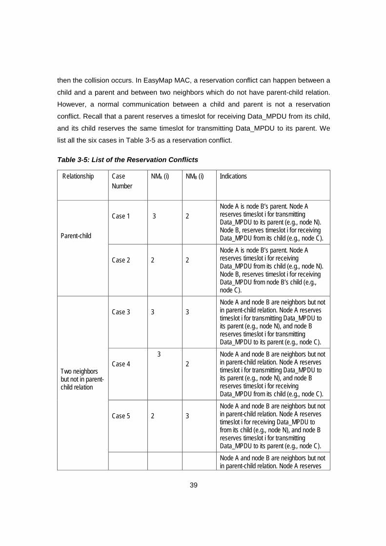
39
then the collision occurs. In EasyMap MAC, a reservation conflict can happen between a
child and a parent and between two neighbors which do not have parent-child relation.
However, a normal communication between a child and parent is not a reservation
conflict. Recall that a parent reserves a timeslot for receiving Data_MPDU from its child,
and its child reserves the same timeslot for transmitting Data_MPDU to its parent. We
list all the six cases in Table 3-5 as a reservation conflict.
Table 3-5: List of the Reservation Conflicts
Relationship Case Number
NMA (i) NMB (i) Indications
Case 1
3
2
Node A is node B’s parent. Node A reserves timeslot i for transmitting Data_MPDU to its parent (e.g., node N). Node B, reserves timeslot i for receiving Data_MPDU from its child (e.g., node C).
Parent-child
Case 2
2
2
Node A is node B’s parent. Node A reserves timeslot i for receiving Data_MPDU from its child (e.g., node N). Node B, reserves timeslot i for receiving Data_MPDU from node B’s child (e.g., node C).
Case 3
3
3
Node A and node B are neighbors but not in parent-child relation. Node A reserves timeslot i for transmitting Data_MPDU to its parent (e.g., node N), and node B reserves timeslot i for transmitting Data_MPDU to its parent (e.g., node C).
Case 4
3 2
Node A and node B are neighbors but not in parent-child relation. Node A reserves timeslot i for transmitting Data_MPDU to its parent (e.g., node N), and node B reserves timeslot i for receiving Data_MPDU from its child (e.g., node C).
Case 5
2
3
Node A and node B are neighbors but not in parent-child relation. Node A reserves timeslot i for receiving Data_MPDU to from its child (e.g., node N), and node B reserves timeslot i for transmitting Data_MPDU to its parent (e.g., node C).
Two neighbors but not in parent-child relation
Node A and node B are neighbors but not in parent-child relation. Node A reserves
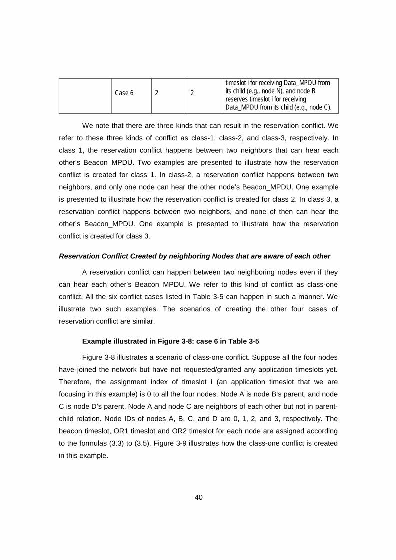
40
Case 6
2
2
timeslot i for receiving Data_MPDU from its child (e.g., node N), and node B reserves timeslot i for receiving Data_MPDU from its child (e.g., node C).
We note that there are three kinds that can result in the reservation conflict. We
refer to these three kinds of conflict as class-1, class-2, and class-3, respectively. In
class 1, the reservation conflict happens between two neighbors that can hear each
other’s Beacon_MPDU. Two examples are presented to illustrate how the reservation
conflict is created for class 1. In class-2, a reservation conflict happens between two
neighbors, and only one node can hear the other node’s Beacon_MPDU. One example
is presented to illustrate how the reservation conflict is created for class 2. In class 3, a
reservation conflict happens between two neighbors, and none of then can hear the
other’s Beacon_MPDU. One example is presented to illustrate how the reservation
conflict is created for class 3.
Reservation Conflict Created by neighboring Nodes that are aware of each other
A reservation conflict can happen between two neighboring nodes even if they
can hear each other’s Beacon_MPDU. We refer to this kind of conflict as class-one
conflict. All the six conflict cases listed in Table 3-5 can happen in such a manner. We
illustrate two such examples. The scenarios of creating the other four cases of
reservation conflict are similar.
Example illustrated in Figure 3-8: case 6 in Table 3-5
Figure 3-8 illustrates a scenario of class-one conflict. Suppose all the four nodes
have joined the network but have not requested/granted any application timeslots yet.
Therefore, the assignment index of timeslot i (an application timeslot that we are
focusing in this example) is 0 to all the four nodes. Node A is node B’s parent, and node
C is node D’s parent. Node A and node C are neighbors of each other but not in parent-
child relation. Node IDs of nodes A, B, C, and D are 0, 1, 2, and 3, respectively. The
beacon timeslot, OR1 timeslot and OR2 timeslot for each node are assigned according
to the formulas (3.3) to (3.5). Figure 3-9 illustrates how the class-one conflict is created
in this example.

41
Figure 3-8: a Scenario of class-one conflict
Figure 3-9: A Class-one conflict creation Procedure
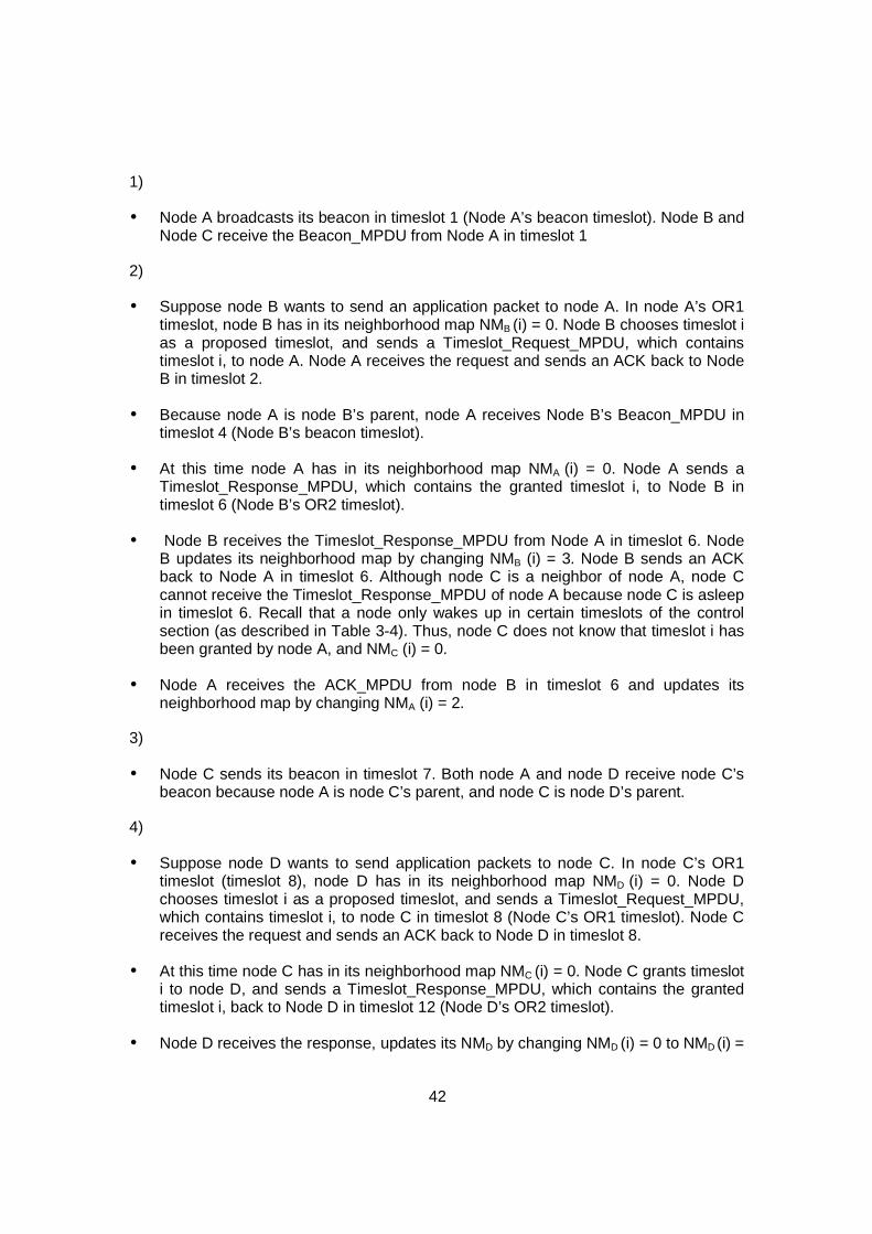
42
1)
Ÿ Node A broadcasts its beacon in timeslot 1 (Node A’s beacon timeslot). Node B and Node C receive the Beacon_MPDU from Node A in timeslot 1
2)
Ÿ Suppose node B wants to send an application packet to node A. In node A’s OR1 timeslot, node B has in its neighborhood map NMB (i) = 0. Node B chooses timeslot i as a proposed timeslot, and sends a Timeslot_Request_MPDU, which contains timeslot i, to node A. Node A receives the request and sends an ACK back to Node B in timeslot 2.
Ÿ Because node A is node B’s parent, node A receives Node B’s Beacon_MPDU in timeslot 4 (Node B’s beacon timeslot).
Ÿ At this time node A has in its neighborhood map NMA (i) = 0. Node A sends a Timeslot_Response_MPDU, which contains the granted timeslot i, to Node B in timeslot 6 (Node B’s OR2 timeslot).
Ÿ Node B receives the Timeslot_Response_MPDU from Node A in timeslot 6. Node B updates its neighborhood map by changing NMB (i) = 3. Node B sends an ACK back to Node A in timeslot 6. Although node C is a neighbor of node A, node C cannot receive the Timeslot_Response_MPDU of node A because node C is asleep in timeslot 6. Recall that a node only wakes up in certain timeslots of the control section (as described in Table 3-4). Thus, node C does not know that timeslot i has been granted by node A, and NMC (i) = 0.
Ÿ Node A receives the ACK_MPDU from node B in timeslot 6 and updates its neighborhood map by changing NMA (i) = 2.
3)
Ÿ Node C sends its beacon in timeslot 7. Both node A and node D receive node C’s beacon because node A is node C’s parent, and node C is node D’s parent.
4)
Ÿ Suppose node D wants to send application packets to node C. In node C’s OR1 timeslot (timeslot 8), node D has in its neighborhood map NMD (i) = 0. Node D chooses timeslot i as a proposed timeslot, and sends a Timeslot_Request_MPDU, which contains timeslot i, to node C in timeslot 8 (Node C’s OR1 timeslot). Node C receives the request and sends an ACK back to Node D in timeslot 8.
Ÿ At this time node C has in its neighborhood map NMC (i) = 0. Node C grants timeslot i to node D, and sends a Timeslot_Response_MPDU, which contains the granted timeslot i, back to Node D in timeslot 12 (Node D’s OR2 timeslot).
Ÿ Node D receives the response, updates its NMD by changing NMD (i) = 0 to NMD (i) =
43
3, and sends an ACK_MPDU back to Node C in the same timeslot (timeslot 12). Although node A is a neighbor of node C, node A cannot receive the Timeslot_Response_MPDU from node C because node A is asleep in timeslot 12. Recall that a node only wakes up in certain timeslots of the control section (as described in Table 3-4). Thus, node A does not know that timeslot i has been granted by Node C.
Ÿ Node C receives the ACK MDPU of node D and updates its NMC by changing NMC
(i) = 0 to NMC (i) = 2.
Ÿ Figure 3-10 shows that the reservation conflict happens in timeslot i between the two neighbors, node A and node C. Node B transmits Data_MPDUs to Node A in timeslot i, and Node D transmits Data_MPDUs to Node C in timeslot i as well. Because node A and node C each needs to send an ACK_MPDU back to their child for each reception of Data_MPDU, an ACK_MPDU and a Data_MPDU can create collision at node A or node C. For example, Node A is receiving a Data_MPDU from Node B, and at the same time Node C is sending an ACK_MPDU to Node D. Since node A can hear Node C, the collision occurs at node A (as illustrated in Figure 3-10).
5) This collision occurs because of the reservation conflict between nodes A and C. In the case of this example, this conflict is resolved in the following superframe through detection of conflict and reservation cancellation.
Ÿ Immediately prior to node A’s beacon timeslot (timeslot 1) of the subsequent superframe, node C has in its neighborhood map NMC (i) = 2. Node C receives node A’s beacon which contains the assignment index NMA (i) = 2. Because node A and node C are not in parent-child relation, according to neighborhood update rule 1.1, node C detects a conflict of timeslot i, and node C needs to cancel timeslot i.
Ÿ Recall the parent cancellation process presented in section 3.6.2, node C needs to initiate the cancellation of timeslot i. Node C just changes the assignment index of timeslot i to 0.
Ÿ Node D receives its parent, node C’s beacon in node C’s beacon timeslot (timeslot 7). According the received neighborhood map of node C, node D updates its neighborhood map by changing the assignment index of timeslot i to 0 because node C detects an assignment inconsistency of timeslot i.
Ÿ The reservation conflict of timeslot i between node C and node A has been resolved because node C stops using timeslot i for reception.
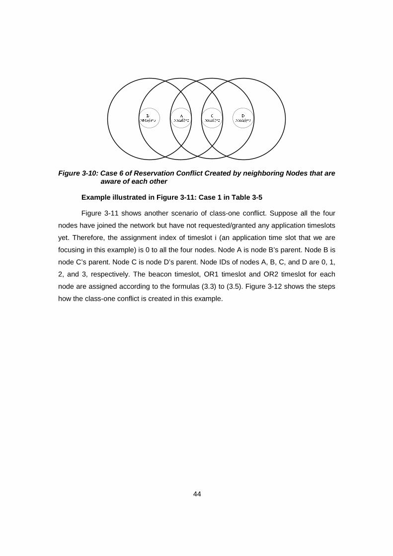
44
Figure 3-10: Case 6 of Reservation Conflict Created by neighboring Nodes that are aware of each other
Example illustrated in Figure 3-11: Case 1 in Table 3-5
Figure 3-11 shows another scenario of class-one conflict. Suppose all the four
nodes have joined the network but have not requested/granted any application timeslots
yet. Therefore, the assignment index of timeslot i (an application time slot that we are
focusing in this example) is 0 to all the four nodes. Node A is node B’s parent. Node B is
node C’s parent. Node C is node D’s parent. Node IDs of nodes A, B, C, and D are 0, 1,
2, and 3, respectively. The beacon timeslot, OR1 timeslot and OR2 timeslot for each
node are assigned according to the formulas (3.3) to (3.5). Figure 3-12 shows the steps
how the class-one conflict is created in this example.

45
Figure 3-11: Another Scenario of Class-one Conflict
Timeslot 1
Timeslot 2
Timeslot 3
Timeslot 4
Timeslot 5
Timeslot 6
Timeslot 7
Timeslot 8
Timeslot 9
Timeslot 10
Timeslot 11
Timeslot 12
Node A’s Beacon timeslot
Node A’s OR1 timeslot
Node A’s OR2 timeslot
Node B’s Beacon timeslot
Node B’s OR1 timeslot
Node B’s OR2 timeslot
Node C’s Beacon timeslot
Node C’s OR1 timeslot
Node C’s OR2 timeslot
Node D’s Beacon timeslot
Node D’s OR1 timeslot
Node D’s OR2 timeslot
Node A’s Beacon
Node A Node B Node C Node D
Timeslot_Request_
ACK
Timeslot_Response
ACK
Node C’s Beacon
Node C’s Beacon
Timeslot_Request
ACK
Timeslot_Response
ACK
… …
Timeslot i
Reserved timeslot for
Transmitting data to node A
Timeslot i
Reserved timeslot for
Receiving data from node B
Timeslot i
Reserved timeslot for
Receiving data from node D
Timeslot i
Reserved timeslot for
Transmitting data to node C
… … … … … …
Data DataData
collision
Node B’s Beacon
Node B’s Beacon
ACK
Figure 3-12: Another Class-one Conflict Creation Procedure
1)
46
Ÿ Node A broadcasts its beacon in timeslot 1.
Ÿ Because node B is node A’s child, node B receives Beacon_MPDU from node A in timeslot 1.
2)
Ÿ Suppose node B wants to send application packets to node A. In node A’s OR1 timeslot, node B has in its neighborhood map NMB (i) = 0. Node B chooses timeslot i as a proposed timeslot, and sends a Timeslot_Request_MPDU, which contains timeslot i, to node A in timeslot 2 (node A’s OR1 timeslot). Node A receives the request and sends an ACK_MPDU back to node B in timeslot 2.
Ÿ Node B sends its Beacon_MPDU in timeslot 4. Node A and node C receive node B’s Beacon_MPDU in timeslot 4 (node B’s beacon timeslot) because node A is node B’s parent, and node C is node B’s child.
Ÿ At this time node A has in its neighborhood map NMA (i) = 0. Node A grants timeslot i to Node B. Node A sends a response, which contains the granted timeslot i, back to node B in timeslot 6 (Node B’s OR2 timeslot). Node B receives the response, updates its NMB by changing NMB (i) = 0 to NMB (i) = 3 and sends an ACK back to Node A in the same timeslot. Node A receives the ACK_MPDU and updates its NMA by changing NMA (i) = 0 to NMA (i) = 2. Although node C is node B’s neighbor, node C does not know that node B has reserved timeslot i because node C was asleep when node B was doing negotiation procedure with node A.
3)
Ÿ Node C sends its beacon in timeslot 7. Node B and node D receive Beacon_MPDU from node C in timeslot 7 because node B is node C’s parent, and node D is node C’s child.
4)
Ÿ Suppose node D wants to send application packets to node C. In node C’s OR1 timeslot (timeslot 8), node D has in its neighborhood map NMD (i) = 0. Node D chooses timeslot i as a proposed timeslot, and sends a Timeslot_Request_MPDU, which contains timeslot i, to node C in timeslot 8 (Node C’s OR1 timeslot). Node C receives the request and sends an ACK back to node D in timeslot 12.
Ÿ At this time node C has in its neighborhood map NMC (i) = 0. Node C grants timeslot i to node D. Node C sends a response, which contains the granted timeslot i, back to node D in timeslot 12 (Node D’s OR2 timeslot). Node D receives the response, updates its NMD by changing NMD (i) = 0 to NMD (i) = 3 and sends an ACK_MPDU back to Node C in the same timeslot. Node C receives the ACK and updates its NMC by changing NMC (i) = 0 to NMC (i) = 2.
Ÿ Figure 3-13 shows that the reservation conflict happens in timeslot i between two neighbors, node B and node C. Node B transmits Data_MPDUs to node A in
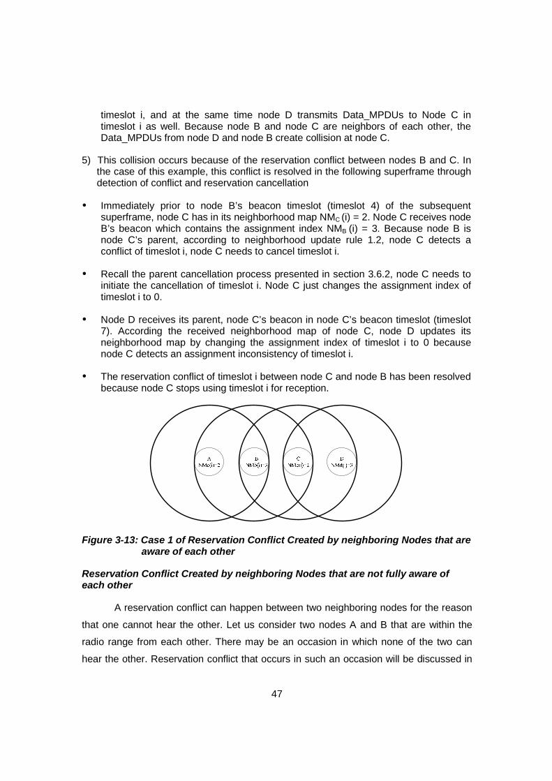
47
timeslot i, and at the same time node D transmits Data_MPDUs to Node C in timeslot i as well. Because node B and node C are neighbors of each other, the Data_MPDUs from node D and node B create collision at node C.
5) This collision occurs because of the reservation conflict between nodes B and C. In the case of this example, this conflict is resolved in the following superframe through detection of conflict and reservation cancellation
Ÿ Immediately prior to node B’s beacon timeslot (timeslot 4) of the subsequent superframe, node C has in its neighborhood map NMC (i) = 2. Node C receives node B’s beacon which contains the assignment index NMB (i) = 3. Because node B is node C’s parent, according to neighborhood update rule 1.2, node C detects a conflict of timeslot i, node C needs to cancel timeslot i.
Ÿ Recall the parent cancellation process presented in section 3.6.2, node C needs to initiate the cancellation of timeslot i. Node C just changes the assignment index of timeslot i to 0.
Ÿ Node D receives its parent, node C’s beacon in node C’s beacon timeslot (timeslot 7). According the received neighborhood map of node C, node D updates its neighborhood map by changing the assignment index of timeslot i to 0 because node C detects an assignment inconsistency of timeslot i.
Ÿ The reservation conflict of timeslot i between node C and node B has been resolved because node C stops using timeslot i for reception.
Figure 3-13: Case 1 of Reservation Conflict Created by neighboring Nodes that are aware of each other
Reservation Conflict Created by neighboring Nodes that are not fully aware of each other
A reservation conflict can happen between two neighboring nodes for the reason
that one cannot hear the other. Let us consider two nodes A and B that are within the
radio range from each other. There may be an occasion in which none of the two can
hear the other. Reservation conflict that occurs in such an occasion will be discussed in

48
later section. In this section, we discuss the case in which only one node can hear the
other. We refer to this kind of conflict as class-two conflict. Without loss of generality, let
us assume that node B recognizes node A as its neighbor but node B does not
recognize node A. That is, node B can hear node A’s beacon but node A cannot hear
node B’s beacon. For example, recall that node A performs a full superframe scan to
receive all its neighbors’ beacons when it is joining the network. In the scanning process,
node A recognizes its neighbors by receiving its neighbors’ beacons, and node A knows
which control timeslots it needs to wake up. However, node A is not able to be aware of
its new neighbor, node B, after node A joins the network because node B had not been
turned on when node A was scanning the full superframe. After node B joins the network,
node B broadcasts its beacon. Although node B is node A’s neighbor, node A does not
listen to node B’s beacon because node A does not know node B as its neighbor. The
reservation conflict can happen between node A and node B because node A does not
have the perception of node B’s timeslot assignments. Four of the six conflict cases
listed in Table 3-5 can happen in such a manner. We illustrate one such example. The
scenarios of creating the other three cases of reservation conflict are similar.
Example illustrated in Figure 3-14: case 4 in Table 3-5
Figure 3-14 shows a scenario of class-two conflict. Suppose node A, node B,
and node D have joined the network but have not granted/requested any application
timeslot. Node C is joining the network. Therefore, the assignment index of timeslot i (an
application timeslot that we are focusing in this example) is 0 to all the four nodes. Node
B is node D’s parent. Node IDs of nodes A, B, C, and D are 0, 1, 2, and 3, respectively.
The beacon timeslot, OR1 timeslot and OR2 timeslot for each node are assigned
according to the formulas (3.3) to (3.5). Figure 3-15 illustrates how the class-two conflict
happens after node C joins the network.
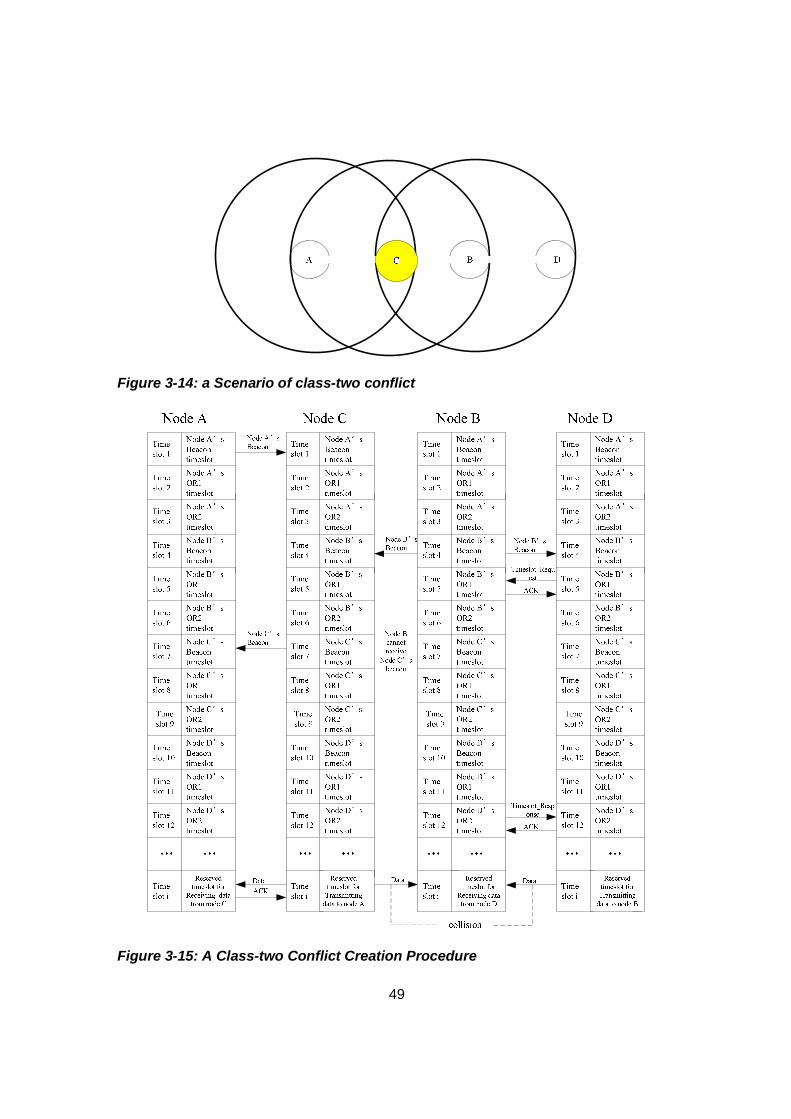
49
Figure 3-14: a Scenario of class-two conflict
Figure 3-15: A Class-two Conflict Creation Procedure

50
1)
Ÿ Node C wants to join the network. Node C performs a full superframe scan.
Ÿ Node C receives node A’s beacon in timeslot 1. In accordance with the first-beacon policy (as described in joining procedure in section 3.4), node C joins node A as its parent after it finishes the scanning process.
Ÿ In the scanning process, node C also receives node B’s beacon in timeslot 4 (node B’s beacon timeslot). After the full superframe scan, node C is aware of two neighbors, node A and node B. Node C joins node A as its parent. Node B is a neighbor of node C, but they are not in parent-child relation. Node A becomes node C’s parent, thus node A knows node C as its neighbor. Node A wakes up in node C’s beacon timeslot and OR2 timeslot (as described in Table 3-4). But node B does not know node C as its neighbor because node B only recognized its neighbors when node B was scanning the whole superframe in the joining procedure (as described in section 3.4).
2)
Ÿ After node C joined the network, suppose that node C wants to send application packets to node A. In node A’s OR1 timeslot, node C has in its neighborhood map NMC(i) = 0. Node C selects timeslot i as a proposed timeslot, and node C sends a Timeslot_Request_MPDU, which contains timeslot i, to node A in timeslot 2 (node A’s OR1 timeslot). Node A receives the request and sends an ACK back to node C in timeslot 2.
Ÿ At this time node A has in its neighborhood map NMA (i) = 0. Node A sends a Timeslot_Response_MPDU, which contains the granted timeslot i, to node C in timeslot 9 (node C’s OR2 timeslot). Node C receives the response and sends an ACK back to node A. Node C updates its neighborhood map by changing the NMC (i) = 0 to NMC (i) = 3.
Ÿ Node A receives the ACK from node C in timeslot 9, and updates its neighborhood map by changing the NMA (i) = 0 to NMA (i) = 2.
3)
Ÿ After a couple of superframes (e.g., 3 superframes later), suppose that node D wants to send application packets to node B. In node B’s OR1 timeslot, node D has in its neighborhood map NMD (i) = 0. .Node D chooses timeslot i as a proposed timeslot, and node D sends a Timeslot_Request_MPDU, which contains timeslot i, to node B in timeslot 5 (node B’s OR1 timeslot). Node B receives the request from node D and sends an ACK back to node D in timeslot 5.
Ÿ Although timeslot i has been assigned to node C for transmission, node B assumes timeslot i is available because node C is a new neighbor of node B, and node B cannot receive node C’s beacon. Node B sends a Timeslot_Response_MPDU, which contains the granted timeslot i, to node D in timeslot 12 (node D’s OR2

51
timeslot)..Node D receives the response and sends an ACK back to node B in timeslot 12. Node D updates its neighborhood map by changing the NMD (i) = 0 to NMD (i) = 3.
Ÿ Node B receives the ACK from node D in timeslot 12, and updates its neighborhood map by changing the NMB (i) = 0 to NMB (i) = 2.
4)
Ÿ From Figure 3-16 we can see that node C is using timeslot i for transmission, and node B is using timeslot i for reception. When node B is receiving a Data_MPDU form node D, at the same time node B can hear the Data_MPDU of node C, the collision occurs at node B.
5) This collision occurs because of the reservation conflict between nodes B and C. In the case of this example, this conflict is resolved in the following superframe through detection of conflict and reservation cancellation
Ÿ Immediately prior to node B’s beacon timeslot (timeslot 4) of the subsequent superframe, say superframe f, node C has in its neighborhood map NMC (i) = 3. Node C receives node B’s beacon which contains the assignment index NMB (i) = 2. Because node B and node C are not parent-child relation, according to the neighborhood update rule 1.1, node C detects a conflict of timeslot i, node C needs to cancel timeslot i.
Ÿ Recall the child cancellation process presented in section 3.6.1, node C needs to send a Timeslot_Cancellation_MPDU, which contains timeslot i as a cancelling timeslot, to node A in node A’s OR1 timeslot (timeslot 2) of superframe f+1. After node C sends the Timeslot_Cancellation_MPDU to node A in timeslot 2 of superframe f+1, node C updates its neighborhood map by changing NMC (i) = 3 to NMC (i) = 0.
Ÿ Node A receives the Timeslot_Cancellation_MPDU, which contains the cancelling timeslot i, from node C in node A’s OR1 of superframe f+1. Node A updates its neighborhood map by changing NMA (i) = 2 to NMA (i) = 0.
Ÿ The reservation conflict of timeslot i between node C and node B has been resolved because node C stops using timeslot i for reception.
The class-two conflict can be resolved through detection of conflict and
reservation cancellation but the conflict can happen repeatedly. In above example, after
the conflict of timeslot i is resolved by node C, suppose node C reserves another
timeslot j. Because node B cannot receive node C’s beacon, node B might reserve
timeslot j as well, and thus the class-two conflict occurs again. To prevent the class-two
conflicts happening repeatedly, we introduce an additional protocol function, which we
call ‘periodic full control section scan’. We describe the process of the periodic full
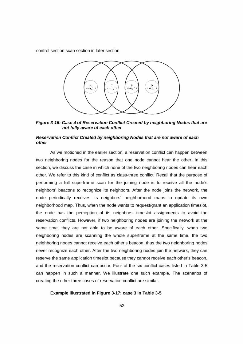
52
control section scan section in later section.
Figure 3-16: Case 4 of Reservation Conflict Created by neighboring Nodes that are not fully aware of each other
Reservation Conflict Created by neighboring Nodes that are not aware of each other
As we motioned in the earlier section, a reservation conflict can happen between
two neighboring nodes for the reason that one node cannot hear the other. In this
section, we discuss the case in which none of the two neighboring nodes can hear each
other. We refer to this kind of conflict as class-three conflict. Recall that the purpose of
performing a full superframe scan for the joining node is to receive all the node’s
neighbors’ beacons to recognize its neighbors. After the node joins the network, the
node periodically receives its neighbors’ neighborhood maps to update its own
neighborhood map. Thus, when the node wants to request/grant an application timeslot,
the node has the perception of its neighbors’ timeslot assignments to avoid the
reservation conflicts. However, if two neighboring nodes are joining the network at the
same time, they are not able to be aware of each other. Specifically, when two
neighboring nodes are scanning the whole superframe at the same time, the two
neighboring nodes cannot receive each other’s beacon, thus the two neighboring nodes
never recognize each other. After the two neighboring nodes join the network, they can
reserve the same application timeslot because they cannot receive each other’s beacon,
and the reservation conflict can occur. Four of the six conflict cases listed in Table 3-5
can happen in such a manner. We illustrate one such example. The scenarios of
creating the other three cases of reservation conflict are similar.
Example illustrated in Figure 3-17: case 3 in Table 3-5
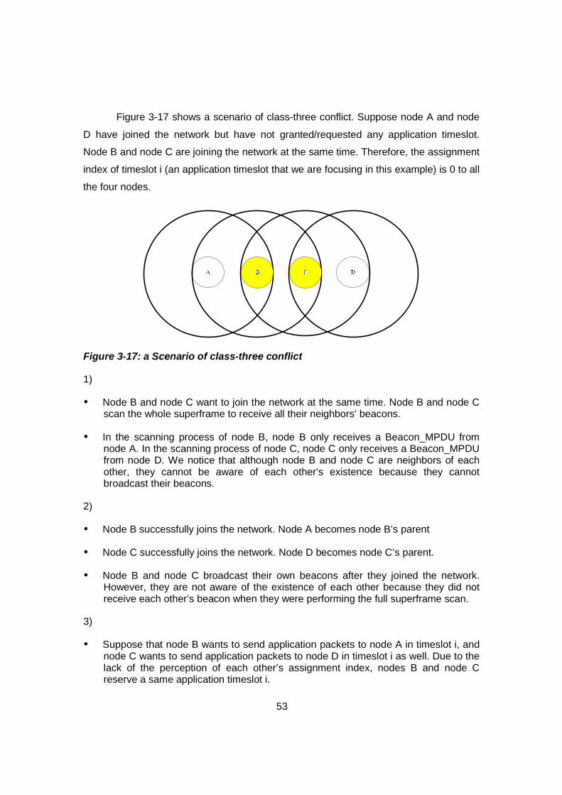
53
Figure 3-17 shows a scenario of class-three conflict. Suppose node A and node
D have joined the network but have not granted/requested any application timeslot.
Node B and node C are joining the network at the same time. Therefore, the assignment
index of timeslot i (an application timeslot that we are focusing in this example) is 0 to all
the four nodes.
Figure 3-17: a Scenario of class-three conflict
1)
Ÿ Node B and node C want to join the network at the same time. Node B and node C scan the whole superframe to receive all their neighbors’ beacons.
Ÿ In the scanning process of node B, node B only receives a Beacon_MPDU from node A. In the scanning process of node C, node C only receives a Beacon_MPDU from node D. We notice that although node B and node C are neighbors of each other, they cannot be aware of each other’s existence because they cannot broadcast their beacons.
2)
Ÿ Node B successfully joins the network. Node A becomes node B’s parent
Ÿ Node C successfully joins the network. Node D becomes node C’s parent.
Ÿ Node B and node C broadcast their own beacons after they joined the network. However, they are not aware of the existence of each other because they did not receive each other’s beacon when they were performing the full superframe scan.
3)
Ÿ Suppose that node B wants to send application packets to node A in timeslot i, and node C wants to send application packets to node D in timeslot i as well. Due to the lack of the perception of each other’s assignment index, nodes B and node C reserve a same application timeslot i.
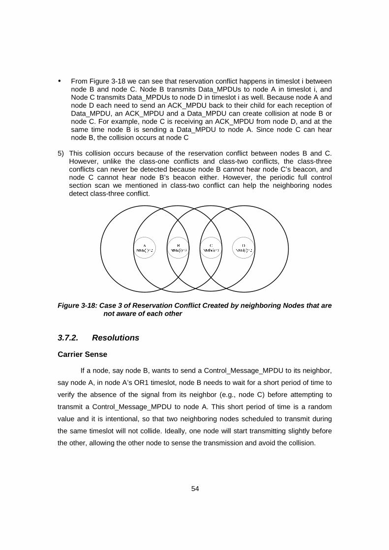
54
Ÿ From Figure 3-18 we can see that reservation conflict happens in timeslot i between node B and node C. Node B transmits Data_MPDUs to node A in timeslot i, and Node C transmits Data_MPDUs to node D in timeslot i as well. Because node A and node D each need to send an ACK_MPDU back to their child for each reception of Data_MPDU, an ACK_MPDU and a Data_MPDU can create collision at node B or node C. For example, node C is receiving an ACK_MPDU from node D, and at the same time node B is sending a Data_MPDU to node A. Since node C can hear node B, the collision occurs at node C
5) This collision occurs because of the reservation conflict between nodes B and C. However, unlike the class-one conflicts and class-two conflicts, the class-three conflicts can never be detected because node B cannot hear node C’s beacon, and node C cannot hear node B’s beacon either. However, the periodic full control section scan we mentioned in class-two conflict can help the neighboring nodes detect class-three conflict.
Figure 3-18: Case 3 of Reservation Conflict Created by neighboring Nodes that are not aware of each other
3.7.2. Resolutions
Carrier Sense
If a node, say node B, wants to send a Control_Message_MPDU to its neighbor,
say node A, in node A’s OR1 timeslot, node B needs to wait for a short period of time to
verify the absence of the signal from its neighbor (e.g., node C) before attempting to
transmit a Control_Message_MPDU to node A. This short period of time is a random
value and it is intentional, so that two neighboring nodes scheduled to transmit during
the same timeslot will not collide. Ideally, one node will start transmitting slightly before
the other, allowing the other node to sense the transmission and avoid the collision.
55
If a node senses a busy channel, then the node cancels the transmission and
may optionally try again at the next superframe (if necessary). A backoff is not required
because before transmitting at the next superframe, the node will perform the carrier
sense again and there is no harm in not backing off.
Exponential Backoff
Carrier sensing will not help avoid the collision happening in the second scenario
of the collision in node’s OR1 timeslot. Thus, we use exponential backoff to detect and
resolve the collision.
The basic idea is that if a node, say node B does not receive an ACK_MPDU
from the receiving node, say node A, after node B sends a Control_Message_MPDU to
node A. Node B will assume that the collision occurs at node A, although there might be
not the collision at node A. For example, the Control_Message_MPDU sent by node B is
lost or the ACK_MPDU sent by node A is lost. Node B may attempt to retry after
executing a binary exponential backoff. The maximum backoff duration is an operational
parameter, but it is important to note that the backoffs occur over superframes, and the
collision resolution process may take several minutes.
Resolution for the class-one/class two conflicts、
The class-one and class-two conflicts can be resolved by detection of conflict
and reservation cancellation. A node, say node B, can detect the conflict by receiving the
newer neighborhood maps from its neighbors in the following superframe. According to
the neighborhood update rules 1.1-1.3, when node B is receiving its neighbors’ beacons,
node B can detect if there is any conflict by checking its own assignment indexes and its
neighbors’ assignment indexes. If node B detects a conflicting timeslot, node B needs to
perform a cancellation process to cancel the conflicting timeslot (as described in section
3.6). After node B cancels the conflicting timeslot, the reservation conflict is resolved
because node B stops using the conflicting timeslot for transmission or reception.
Periodic Full Control Section Scan
“Periodic full control section scan” is a node’s activity of waking up for the full
control section periodically to update the perception of its neighbors. In a full control
56
section scanning process, a node can be aware of one or some new neighbors.
Because a node does not know when a new neighboring node joins the network, the
node needs to perform the full control section scan periodically. The periodic full control
section scan can prevent the class-two conflicts happening repeatedly, it also helps the
neighboring nodes detect the class-three conflicts.
The class-two conflicts can be resolved without the periodic full control section
scan, but the periodic full control section scan can prevent the class-two conflicts
happening repeatedly. Recall the example of Figure 3-14, although node C can resolve
the conflict by detecting the conflict of timeslot i and cancelling timeslot i, the conflict can
happen again if node B reserves another timeslot (e.g., timeslot j) that has been
assigned to node C. However, when node B is performing the full control section scan,
node B can receive node C’s beacon, and node B recognizes node C as its new
neighbor. Thus, by receiving node C’s beacon, node B has the perception of node C’s
timeslot assignments, and node B will not request/grant the timeslot that has been
assigned to node C. The class-two conflicts will not occur again between node B and
node C.
The class-three conflicts cannot be detected without the full control section scan
because none of the two neighboring nodes can hear each other’s beacon. Recall the
example of Figure 3-17, node C and node B can never hear each other’s beacon, thus
the conflict can never be detected. However, if node B and node C perform a full control
section scan, node B and node C become aware of each other and they can receive
each other’s beacon. From the received beacon of each other, node B and node C can
detect the conflict according to the neighborhood update rule 1.1. After a node (either
node B or node C) detects timeslot i as a conflicting timeslot, the node needs to cancel
the conflicting timeslot. Thus, not only can the periodic full control section scan prevent
the class-two conflicts, but also detect the class-three conflicts.
The frequency of performing a full control section scan has not been defined yet.
However, this parameter should not be concerned too much in EasyMap MAC because
the scanning node only needs to be awake for the entire control section. The control
section only lasts for one second rather than the entire superframe. Thus, performing a
full control section scan will not increase the duty cycle too much. Besides, the scanning
57
node can still receive and transmit Data_MPDUs in the application section. The
throughput should not be affected at all.
3.8. Dead Lock and Unlock Process
In EasyMap MAC, an application timeslot deadlock is when an application
timeslot, say timeslot i, cannot be assigned to a node, say node B, even none of node
B’s neighbor is using timeslot i for transmission or reception. Specifically, an application
timeslot, say timeslot i, is reserved between a parent, say node A, and a child, say node
B, during the negotiation process. The assignment index of timeslot i becomes 3 for the
child and 2 for the parent. However, a neighboring node of node A, say node C, also
becomes aware of the successful reservation by listening to node A’s beacon, thus the
assignment of timeslot i becomes 1 for node C. Recall that reserved timeslot i can also
be cancelled by either node A or node B due to a specific reason. After timeslot i is
cancelled by node A and node B, the assignment index of the cancelled timeslot i
becomes 0 for both node A and node B. Because of the neighborhood map update rules,
there is no provision for resetting an assignment index to zero other than as a part of the
negotiation procedure. The assignment index of timeslot i for node C cannot reset back
to zero, and the timeslot i cannot be assigned to node C forever. Eventually all nodes will
run out of free application timeslots because of the application timeslot deadlocks.
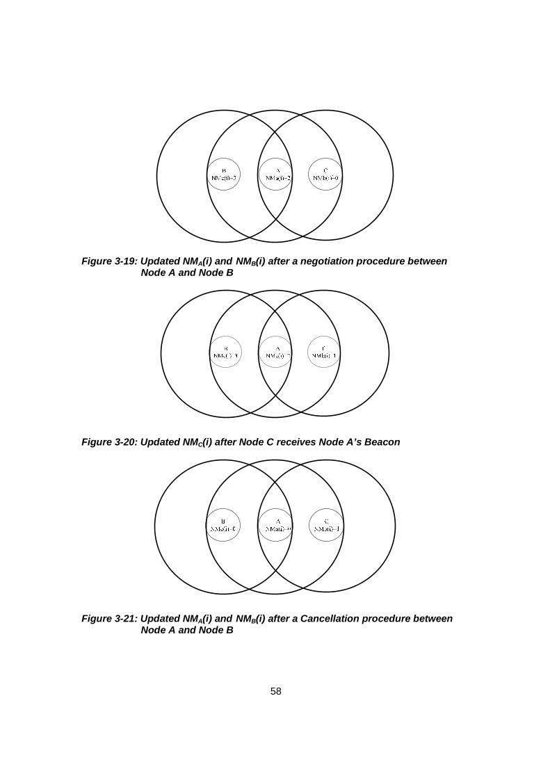
58
Figure 3-19: Updated NMA(i) and NMB(i) after a negotiation procedure between Node A and Node B
Figure 3-20: Updated NMC(i) after Node C receives Node A’s Beacon
Figure 3-21: Updated NMA(i) and NMB(i) after a Cancellation procedure between Node A and Node B
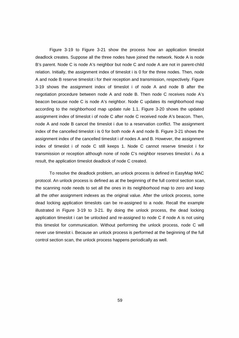
59
Figure 3-19 to Figure 3-21 show the process how an application timeslot
deadlock creates. Suppose all the three nodes have joined the network. Node A is node
B’s parent. Node C is node A’s neighbor but node C and node A are not in parent-child
relation. Initially, the assignment index of timeslot i is 0 for the three nodes. Then, node
A and node B reserve timeslot i for their reception and transmission, respectively. Figure
3-19 shows the assignment index of timeslot i of node A and node B after the
negotiation procedure between node A and node B. Then node C receives node A’s
beacon because node C is node A’s neighbor. Node C updates its neighborhood map
according to the neighborhood map update rule 1.1. Figure 3-20 shows the updated
assignment index of timeslot i of node C after node C received node A’s beacon. Then,
node A and node B cancel the timeslot i due to a reservation conflict. The assignment
index of the cancelled timeslot i is 0 for both node A and node B. Figure 3-21 shows the
assignment index of the cancelled timeslot i of nodes A and B. However, the assignment
index of timeslot i of node C still keeps 1. Node C cannot reserve timeslot i for
transmission or reception although none of node C’s neighbor reserves timeslot i. As a
result, the application timeslot deadlock of node C created.
To resolve the deadlock problem, an unlock process is defined in EasyMap MAC
protocol. An unlock process is defined as at the beginning of the full control section scan,
the scanning node needs to set all the ones in its neighborhood map to zero and keep
all the other assignment indexes as the original value. After the unlock process, some
dead locking application timeslots can be re-assigned to a node. Recall the example
illustrated in Figure 3-19 to 3-21. By doing the unlock process, the dead locking
application timeslot i can be unlocked and re-assigned to node C if node A is not using
this timeslot for communication. Without performing the unlock process, node C will
never use timeslot i. Because an unlock process is performed at the beginning of the full
control section scan, the unlock process happens periodically as well.

60
4. Evaluation
This chapter provides two sets of simulation results and their analysis. In the first
set of simulations, we compare the performance of IEEE 802.15.4 and EasyMap MAC
protocols in similar environments. We use packet delivery ratio as the performance
metric. The simulation results show the packet delivery ratios of IEEE 802.15.4 and
EasyMap MAC protocol at different traffic loads (from light to heavy). In the second set
of simulations, we focus on the performances of EasyMap MAC for a particular
application; namely, a Bridge Health Monitoring system.
4.1. Comparison between IEEE 802.15.4 and EasyMap MAC
In the first set of simulations, our objective is to compare the packet delivery ratio
(or, 1 minus packet drop probability)3 and the duty cycle of IEEE 802.15.4 and EasyMap
MAC protocol at different traffic loads. As the duty cycle and the packet delivery ratio will
have tradeoffs, our objective is to compare the packet delivery ratio of EasyMap with that
of IEEE 802.15.4 associated with the similar duty cycle at the same traffic load. We use
different traffic loads (from light to heavy) to test the performance of the packet delivery
ratio for IEEE 802.15.4 and EasyMap MAC protocol.
Recall that for IEEE 802.15.4, the duty cycle can be set by configuring two
parameters − BO (Beacon Order) and SO (Superframe Order). For EasyMap MAC
protocol, the duty cycle cannot be pre-set because the timeslot reservation decisions are
distributed, and each node dynamically makes timeslot reservations through negotiation
with its neighbors in response to the traffic condition of the node in accordance with its
time slot reservation policy. In fact, the timeslot reservation policy is not a part of the
3 We examine the system in which there is no retransmission of packets dropped due to
buffer overflow.
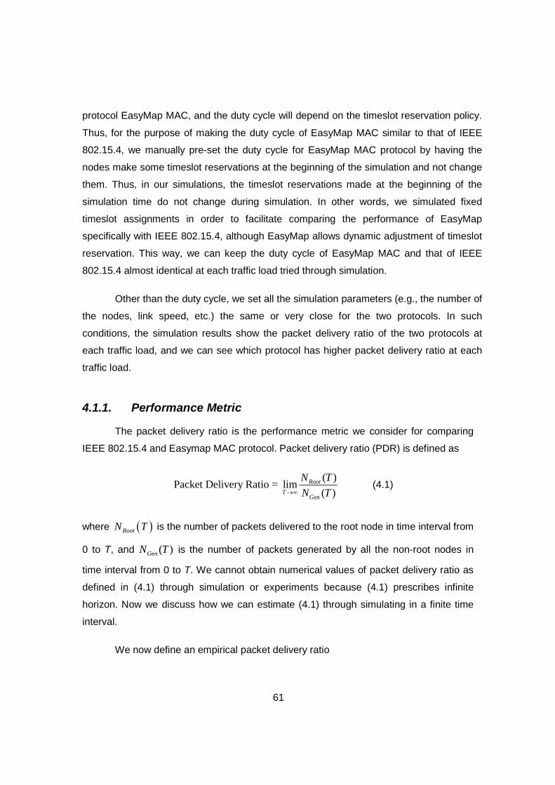
61
protocol EasyMap MAC, and the duty cycle will depend on the timeslot reservation policy.
Thus, for the purpose of making the duty cycle of EasyMap MAC similar to that of IEEE
802.15.4, we manually pre-set the duty cycle for EasyMap MAC protocol by having the
nodes make some timeslot reservations at the beginning of the simulation and not change
them. Thus, in our simulations, the timeslot reservations made at the beginning of the
simulation time do not change during simulation. In other words, we simulated fixed
timeslot assignments in order to facilitate comparing the performance of EasyMap
specifically with IEEE 802.15.4, although EasyMap allows dynamic adjustment of timeslot
reservation. This way, we can keep the duty cycle of EasyMap MAC and that of IEEE
802.15.4 almost identical at each traffic load tried through simulation.
Other than the duty cycle, we set all the simulation parameters (e.g., the number of
the nodes, link speed, etc.) the same or very close for the two protocols. In such
conditions, the simulation results show the packet delivery ratio of the two protocols at
each traffic load, and we can see which protocol has higher packet delivery ratio at each
traffic load.
4.1.1. Performance Metric
The packet delivery ratio is the performance metric we consider for comparing
IEEE 802.15.4 and Easymap MAC protocol. Packet delivery ratio (PDR) is defined as
en
( )Packet Delivery Ratio = lim
( )Root
TG
N TN T®¥
(4.1)
where ( )RootN T is the number of packets delivered to the root node in time interval from
0 to T, and e ( )G nN T is the number of packets generated by all the non-root nodes in
time interval from 0 to T. We cannot obtain numerical values of packet delivery ratio as
defined in (4.1) through simulation or experiments because (4.1) prescribes infinite
horizon. Now we discuss how we can estimate (4.1) through simulating in a finite time
interval.
We now define an empirical packet delivery ratio

62
( ) ( )( ) ( )en
Packet Delivery Ratio for Simulations PDRS Root
G Buffer
N T
N T N T=
- (4.2)
which can be obtained from simulation to estimate packet delivery ratio (4.1). In
(4.2) T is the length of our simulation duration. ( )RootN T is the number of packets
delivered to the root node in time interval from 0 to T. e ( )G nN T is the number of packets
generated by all the non-root nodes in time interval from 0 to T. ( )BufferN T is the number
of packets still in the buffer when simulation duration fires, and we subtract ( )BufferN T
from e ( )G nN T because some data packets can be still in the buffer at the end of
simulation for a finite length of time T. We do not really know whether or not those data
packets in the buffer will be delivered to the root node successfully.
However, if T is not sufficiently long, even (4.2) is not an accurate estimation of
(4.1) because the buffers are all empty at the beginning of simulations. In Appendix C,
we discuss the method we used to estimate (4.1) reasonably well in relatively short
simulation time.
4.1.2. Simulation Setup
Simulation Tool and Modules
To perform our comparison of the packet delivery ratio between IEEE 802.15.4
and EasyMap MAC protocol, we conduct our performance simulations on NS2 (Network
Simulator 2) [17] [18]. For IEEE 802.15.4, we modified the original IEEE 802.15.4
module [19] available in NS2. The original NS 802.15.4 module does not support multi-
hop topologies as IEEE 802.15.4 does not define a beacon scheduling mechanism for
multi-hop topologies. Thus we cannot simulate the original NS 802.15.4 module for a
multi-hop topology. To evaluate the performance of IEEE 802.15.4 on a multi-hop
topology, we first designed a beacon scheduling mechanism for IEEE 802.15.4. The
beacon scheduling mechanism is specially designed for the linear topology presented in
Figure 4-1, and it may not support other IEEE 802.15.4 multi-hop topologies. Then, we
integrated the beacon scheduling mechanism with the original module of IEEE 802.15.4.
That way, we can simulate the modified IEEE 802.15.4 module for the multi-hop

63
topology. The beacon mechanism we designed is presented in Appendix B. To evaluate
the performance of EasyMap MAC protocol, we developed our own EasyMap MAC
module on NS2, and we present the results of EasyMap MAC by simulating the
EasyMap MAC module.
Simulation Configurations
To see the performance of packet delivery ratio of IEEE 802.15.4 and EasyMap
MAC protocol at different traffic loads, we simulate seven different traffic loads for both
two protocols. The nodes generate data packets at seven traffic loads, which are 0.5
packet/s, 0.6 packet/s, 0.7packet/s, 0,8 packet/s, 0.9 packet/s, 1.0 packet/s and 2.0
packets/s. The traffic type is periodic. For example, if we set the exogenous traffic
generated at a node to l packet/s, then a packet arrives at the node periodically at every
1/l second. We set the buffer size of each node to 100 data packets, and each data
packet has length 25bytes. In terms of the routing rule, in the linear physical topology
illustrated in Fig. 4.1, all the data packets from a non-root node must be transmitted to
its parent, and then forwarded to the upstream. In our simulations, the physical
transmission rate is 250 kb/s.
We use seven traffic loads to evaluate the performance of EasyMap MAC and
IEEE 802.15.4. At each traffic load, 10 independent simulations are performed for both
the modified IEEE 802.15.4 module and EasyMap MAC module. Each independent
simulation lasts for 3600seconds. The results presented in section 4.1.3 are averaged
over all the ten different simulations.
We consider a linear physical topology, which is illustrated in Figure 4-1. The
physical network topology consists of 9 nodes − one root node and the eight non-root
nodes. We assume that the root node (node 0 in Figure 4-1) is mains powered, so the
network can operate, with the root node being always awake. The non-root nodes (node
1 through node 8 in Figure 4-1) operate with a duty cycle for power management.

64
1 0 2 3 8 7 6 5 4
Figure 4-1: A Linear Network Topology of the first set of simulations
IEEE 802.15.4 specifies the typical operating range is from 10 meters to 75
meters [20]. In this set of simulations, we suppose that the nodes operate with a radio
range of 10 meters. In Figure 4-1, we set the distance between any two neighboring
nodes to be slightly less than but close to 10 meters so that the node can only receive
its neighbors’ packet. We assume that the node (e.g., node 1) can receive its (e.g., node
1’s) neighbors’ packet (node 0’s ACK or node 2’s data packet) without any error (error-
free reception).
As for the duty cycle, recall that the duty cycle of IEEE 802.15.4 is determined by
BO (Beacon Order) and SO (Superframe Order). We calculated the Beacon Interval (BI)
and the Superframe Duration (SD) by using formula (4.3) and (4.4), respectively.
The Beacon Interval of IEEE 802.15.4 is defined as
*2BOBI aBaseSuperframeDuration symbols= (4.3)
where IEEE 802.15.4 defines aBaseSuperframeDuration to be 960 symbol durations [1,
p.159]. BO stands for the Beacon Order, which specifies the length of the beacon
interval. IEEE 802.15.4 specifies that we can choose any integer from [0, 14] as the BO.
In our simulations, we choose 9 as the Beacon Order.
The Superframe Duration of IEEE 802.15.4 is defined as
*2SOSD aBaseSuperframeDuration symbols= (4.4)
where SO stands for the Superframe Order, which specifies the length of the
superframe duration. IEEE 802.15.4 specifies that we can choose any integer from

65
[0,BO] as the SO. We set the SO to 5 in the simulations. Thus, the corresponding duty
cycle, SD/BI, is 6.25%.
We also pre-set the duty cycle of EasyMap MAC protocol by having the nodes
make some timeslot reservations at the beginning of the simulations and not change
them. The duty cycle we pre-set for EasyMap MAC is very similar to that of IEEE
802.15.4. We assume that node 0 is mains powered and that the duty cycle of node 0 is
100%. The duty cycle of EasyMap MAC protocol can be calculated as the average duty
cycle of the nodes (node 1 through node 8). We denote by Duty(i) the duty cycle of node
i,i=1,…,8. Then, we have
( )
_ _ _ __ _
Duty i
Control timeslot Length NC Application timeslot Length NALength of Superframe
=´ + ´ (4.5)
where the Control_timeslot_Length denotes the length of the control timeslot,
Application_timeslot_Length represents the length of the application timeslot, NA
denotes the number of application timeslots at which the node is awake in the
superframe, and NC denotes the number of control timeslots at which the node is awake
in the superframe. The Length_of_Superframe denotes the length of the superframe in
EasyMap MAC.
We set the length of the control timeslot to 3.38ms, the length of the application
timeslot to 31.25ms, and the length of the superframe to 8s.
In the example of Figure 4-1, NC is 5 for node 8. Node 8 needs to wake up at its
own three control timeslots, which are node 8’s Beacon timeslot, OR1 timeslot, and OR2
timeslot. Node 8 also needs to wake up at its parent’s (node 7’s) two control timeslots,
which are node 7’s Beacon timeslot and OR1 timeslot.
Each node except the nodes at the ends (node 0 and node 8) needs to wake up
at seven control timeslots; that is, each of them has value NC = 7. Specifically, the node
wakes up at its own three control timeslots, which are the node’s Beacon timeslot, OR1
timeslot, and OR2 timeslot. The node needs to wake up at its parent’s two control
timeslots, which are the parent’s Beacon timeslot and OR1 timeslot. The node also
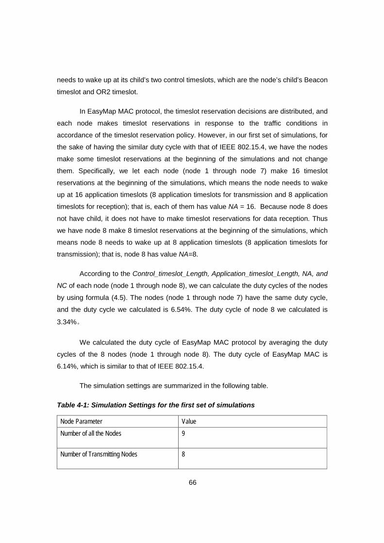
66
needs to wake up at its child’s two control timeslots, which are the node’s child’s Beacon
timeslot and OR2 timeslot.
In EasyMap MAC protocol, the timeslot reservation decisions are distributed, and
each node makes timeslot reservations in response to the traffic conditions in
accordance of the timeslot reservation policy. However, in our first set of simulations, for
the sake of having the similar duty cycle with that of IEEE 802.15.4, we have the nodes
make some timeslot reservations at the beginning of the simulations and not change
them. Specifically, we let each node (node 1 through node 7) make 16 timeslot
reservations at the beginning of the simulations, which means the node needs to wake
up at 16 application timeslots (8 application timeslots for transmission and 8 application
timeslots for reception); that is, each of them has value NA = 16. Because node 8 does
not have child, it does not have to make timeslot reservations for data reception. Thus
we have node 8 make 8 timeslot reservations at the beginning of the simulations, which
means node 8 needs to wake up at 8 application timeslots (8 application timeslots for
transmission); that is, node 8 has value NA=8.
According to the Control_timeslot_Length, Application_timeslot_Length, NA, and
NC of each node (node 1 through node 8), we can calculate the duty cycles of the nodes
by using formula (4.5). The nodes (node 1 through node 7) have the same duty cycle,
and the duty cycle we calculated is 6.54%. The duty cycle of node 8 we calculated is
3.34%。
We calculated the duty cycle of EasyMap MAC protocol by averaging the duty
cycles of the 8 nodes (node 1 through node 8). The duty cycle of EasyMap MAC is
6.14%, which is similar to that of IEEE 802.15.4.
The simulation settings are summarized in the following table.
Table 4-1: Simulation Settings for the first set of simulations
Node Parameter Value
Number of all the Nodes 9
Number of Transmitting Nodes 8

67
Node Physical Topology Linear
Traffic Type Periodic
Exogenous Traffic Load at each node=1,…,8 (packet(s)/second)
0.5, 0.6, 0.7, 0.8, 0.9,1.0,2.0
Packet Size (byte) 25
Radio Range (m) 10
Distance between Two Neighboring Nodes (m)
Slightly less than 10
Buffer Size (packets) 100
SO/BO of node 0 (IEEE 802.15.4) 9/9
SO/BO of the nodes (node 1 through node 8) (IEEE 802.15.4)
5/9
Duty Cycle of IEEE 802.15.4 6.25%
Duty Cycle of Easy MAC 6.14%
Simulation Duration (second) 3600
4.1.3. Simulation Results and Analysis
Figure 4-2 shows the packet delivery ratio of IEEE 802.15.4 at different traffic
loads. Figure 4-2 indicates that for the traffic loads lighter than 0.9 packet/second, the
packet delivery ratios are very high − almost 100%. Figure 4-2 indicates that IEEE
802.15.4 operates very well when the traffic loads are lighter than 0.9packet/second in
our simulation configurations. Then, we simply found that the packet delivery ratio starts
to drop when the traffic load increases to 0.9 packet/second. When the traffic load is 0.9
packet/second, the packet delivery ratio does not drop too much, and it still stays around
96%. After that, with the increase of the traffic load to 1.0 packet/second, the packet
delivery ratio drops about 9%. About 87% data packets are successfully delivered to the
root node in our simulation configurations. Finally, it is easily to point out that over 50%

68
packets are not successfully delivered to the root node when the traffic load is 2.0
packets/second.
Figure 4-2: the Packet delivery ratios of 802.15.4 at the Different Traffic Loads
We also simulated the EasyMap MAC module. The simulation results of
EasyMap MAC are quite different from that of IEEE 802.15.4. For EasyMap MAC,
except for the data packets left in the buffer at the end of the simulation, all the data
packets generated by the non-root nodes were delivered to the root node at all the
seven traffic loads. The NS (Network Simulator) provides the number of packets
dropped due to buffer overflow, and in our EasyMap MAC simulations the number of
dropped packets was zero for all simulation experiments. The packet delivery ratios of
EasyMap MAC are 100% at all the seven traffic loads in our simulations.
When the traffic load is less than 0.9 packet/s, the delivery ratios of IEEE
802.15.4 and EasyMap MAC protocol are very close. Both IEEE 802.15.4 and EasyMap
MAC can operate with very high packet delivery ratio in our simulation configurations.
When the traffic load is 1.0 packet/second, EasyMap MAC protocol keeps a packet
delivery ratio of 100% but the packet delivery ratio of IEEE 802.15.4 decreases to 87%.
When the traffic load is 2.0 packet/second, the packet delivery ratio of IEEE 802.15.4 is
less than 50% but the packet delivery ratio of EasyMap MAC is still 100%.
We simulated seven different traffic loads for IEEE 802.15.4 and EasyMap MAC
protocol in the similar environments. EasyMap MAC protocol has higher packet delivery
ratio than that of IEEE 802.15.4 at all the seven traffic loads in our simulations.
69
4.2. Performances Test of EasyMap MAC on a Bridge Health Monitoring System
In this section, we focus on testing the performances of EasyMap MAC protocol
for a particular network system; namely, a Bridge Health Monitoring System. We used a
particular timeslot reservation policy we designed for the simulations. We focus on three
performance metrics of EasyMap MAC, which are the number of packet drops, packet
delivery ratio, and duty cycle.
4.2.1. Timeslot Reservation Policy Used
In the first set of simulations, to fairly compare EasyMap MAC protocol with IEEE
802.15.4, we pre-set the duty cycle of EasyMap MAC protocol. However, to test the
performances of EasyMap MAC protocol for a Bridge Health Monitoring system, we
consider a dynamic packet reservation policy, which is a natural combination with
EasyMap MAC. The packet reservation policy consists of two parts − the policy that
governs when a node sends a new timeslot reservation request to its parent and the
policy that governs how a node respond to its child’s request for new timeslot
reservation. Different timeslot reservation policies may present different performances of
EasyMap MAC protocol but we only focus on testing the performances of EasyMap
MAC protocol that employs our policy. We leave as future study the design and analysis
of other policies.
In designing our reservation policy, we assume that the traffic load is relatively
low and thus nodes will have sufficient transmission speed (the number of timeslots per
unit time) to forward the data traffic. We also assume that the length of an application
data packet is smaller than or equal to 5% of the buffer size. Let us denote by Q(i,t) the
percentage of available buffer space in node i’s buffer at time t and by U(i,t) the
occupied buffer space in node i’s buffer at time t. If node i has buffer size Buf, we
have ( , )( , ) 100
Buf U i tQ i t
Buf-
= ´ . If Q (B,t ) is lower than 5%, node B, makes one more
timeslot reservation for transmission. When node B requires one more timeslot
reservation, node B sends a Timeslot_Request_MPDU, which contains the list of the
proposed timeslots (e.g., timeslot i, timeslot j,…, timeslot k), to its parent, say node A.
70
Node A decides whether or not to grant an application timeslot to node B. If ( ),Q A t ,
where t is the time when the Timeslot_Request_MPDU is received, is lower than 5%,
node A sends a Timeslot_Response_MPDU that does not contain any granted timeslot,
to node B − that is, the parent does not grant any new timeslot because the parent’s
buffer is almost full. Node B might have to send another Timeslot_Response_MPDU to
node A in the next superframe. If ( ),Q A t is not lower than 5%, node A compares the
proposed timeslots with its own NMA and only select the timeslots whose assignment
index is 0 in node A’s neighborhood map. Among these timeslots, node A randomly
selects only one timeslot (e.g., timeslot i) as the granted timeslot in our policy adopted
for simulation. Then, node A sends a Timeslot_Response_MPDU, which contains the
granted timeslot (e.g., timeslot i), to node B. Then, node B receives the
Timeslot_Response_MPDU, which contains the granted timeslot (e.g., timeslot i) from
node A. Node A and node B successfully made a common timeslot reservation. Node A
has made one timeslot reservation for reception, and node B has made one timeslot
reservation for transmission. We also designed the reservation policy so that nodes
cannot make timeslot reservations for transmission in two consecutive superframes.
Specifically, a node, say node B, is not allowed to make the timeslot reservation for
transmission in the subsequent superframe if node B just made one timeslot reservation
for transmission in the current superframe.
In this simple policy designed for our simulation, a node does not cancel the
timeslots reserved for its transmission, even if the node’s queue length is reduced below
95% of the buffer size. In other words, the number of timeslots reserved for simulation
never decreases. Because the incoming traffic pattern is deterministic (due to periodic
arrivals of exogenous traffic), eventually each node keeps increasing the number of
timeslots it reserves to the point where there will be no more buffer overflow.
4.2.2. Simulation Setup
Simulation Tool and Simulation Module
In our second set of the simulations, which are being presented in this section,
we also conduct our simulations with NS2. Recall that we simulated the EasyMap MAC
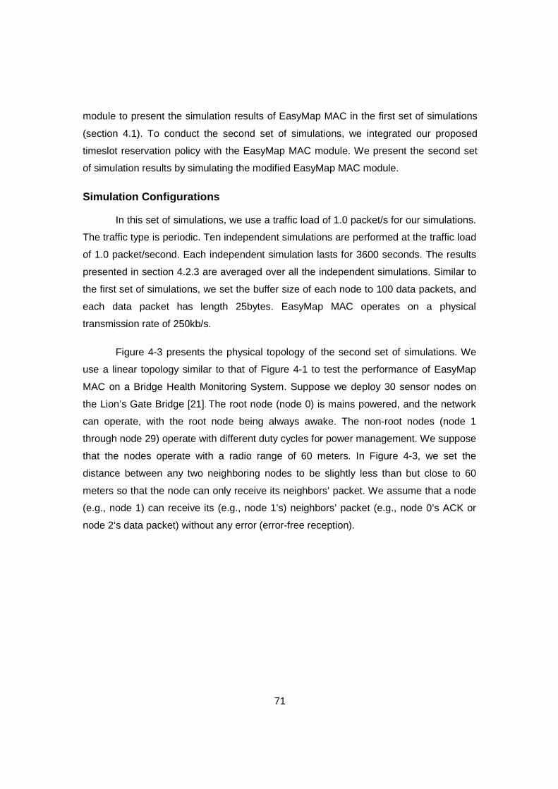
71
module to present the simulation results of EasyMap MAC in the first set of simulations
(section 4.1). To conduct the second set of simulations, we integrated our proposed
timeslot reservation policy with the EasyMap MAC module. We present the second set
of simulation results by simulating the modified EasyMap MAC module.
Simulation Configurations
In this set of simulations, we use a traffic load of 1.0 packet/s for our simulations.
The traffic type is periodic. Ten independent simulations are performed at the traffic load
of 1.0 packet/second. Each independent simulation lasts for 3600 seconds. The results
presented in section 4.2.3 are averaged over all the independent simulations. Similar to
the first set of simulations, we set the buffer size of each node to 100 data packets, and
each data packet has length 25bytes. EasyMap MAC operates on a physical
transmission rate of 250kb/s.
Figure 4-3 presents the physical topology of the second set of simulations. We
use a linear topology similar to that of Figure 4-1 to test the performance of EasyMap
MAC on a Bridge Health Monitoring System. Suppose we deploy 30 sensor nodes on
the Lion’s Gate Bridge [21]. The root node (node 0) is mains powered, and the network
can operate, with the root node being always awake. The non-root nodes (node 1
through node 29) operate with different duty cycles for power management. We suppose
that the nodes operate with a radio range of 60 meters. In Figure 4-3, we set the
distance between any two neighboring nodes to be slightly less than but close to 60
meters so that the node can only receive its neighbors’ packet. We assume that a node
(e.g., node 1) can receive its (e.g., node 1’s) neighbors’ packet (e.g., node 0’s ACK or
node 2’s data packet) without any error (error-free reception).
72
1 0 2 3 29 28 27
Figure 4-3: Linear Topology of the second set of simulations
The simulation settings of the second set of simulations are summarized in the following table.
Table 4-2: Simulation Settings for the second set of simulations
Node Parameter Value
Number of all the Nodes 30
Number of Transmitting Nodes 29
Node Physical Topology Linear
Radio Range 60
Distance between Two Neighboring Nodes(m) Slightly less than 60
Traffic Type Periodic
Exogenous Traffic Load at each node =1,…,29 (packet/second)
1.0
Packet Size (byte) 25
Buffer Size (packets) 100
Total Simulation Duration (second) (SD) 3600
4.2.3. Performance Metrics
In this set of simulations, we present three performance metrics. We will present
the packet delivery ratio, the duty cycle of EasyMap MAC. In addition we present the
number of packet drops.
73
Number of Packet Drops and Packet Delivery Ratio
As in the second set of simulations, we will consider the packet delivery ratio. In
addition, we will consider the number of packet drops in more detail because dynamic
nature of the timeslot reservation policy makes the queue length fluctuation more
unpredictable. In the example of Figure 4-3, we assume that the nodes can receive their
neighbors’ packet without error. The packet drops happen because of the buffer overflow
in our simulations.
As for the packet delivery ratio, as long as the source traffic arrival is periodic and
there is enough timeslots available in each link to handle the traffic, the packet delivery
ratio will be 100%, averaged over the infinite time horizon. The reason is that the
timeslot reservation policy presented in section 4.2.1 will not have any buffer overflows
after some operation time in such deterministic source data generation. Therefore, the
focus of our simulation experimentation will be the amount of data loss due to packet
drops at the early part of operations. In other words, the system will have 0-packet drop
when reaching the steady state and our focus packet loss rate until the system reaches
the steady state. Therefore, we do not discard the first initial transient period for
obtaining the more accurate simulation results. This is a main difference of our
simulation in this section from the simulations presented in section 4.1.
Duty Cycle
Similar to the first set of simulations, the duty cycle of the second set of
simulations is the average duty cycle of the nodes (node 1 through node 29 in Figure 4-
3). However, the duty cycles of the nodes are not pre-set in the second set of
simulations, and we do not have the nodes make any timeslot reservation timeslot at the
beginning of the simulations. Each node dynamically makes timeslot reservations in
response to the traffic conditions of the node in accordance with our timeslot reservation
policy. Recall that node 0 is mains powered, the duty cycle of node 0 is 100%. We use
formula (4.5) to calculate the duty cycles of the nodes (node 1 through node 29 in Figure
4-3) in our second set of simulations. We need to know the NC and NA of each node for
calculating the duty cycle. Similar to the first set of simulations, each node (through node
1 to node 28) wakes up at seven control timeslots, and node 29 wake up at 5 control
timeslots. However, the value of NA of each node (node 1 through node 29) will change
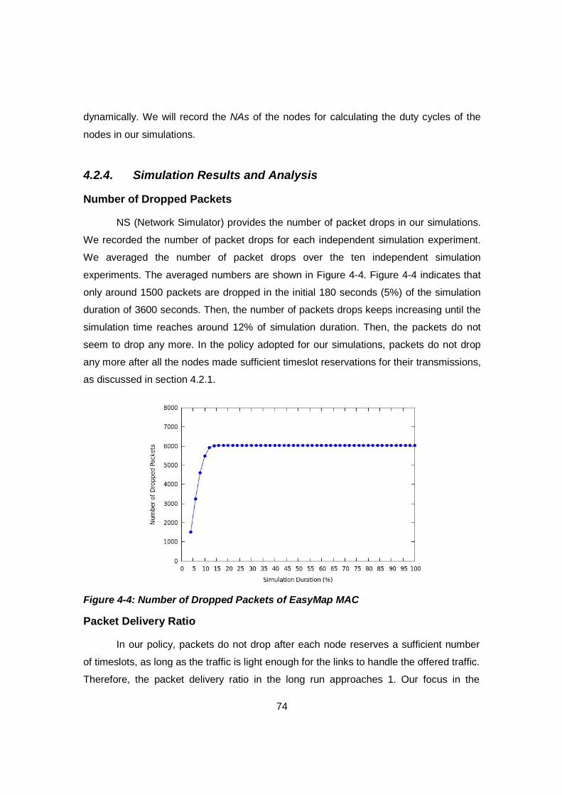
74
dynamically. We will record the NAs of the nodes for calculating the duty cycles of the
nodes in our simulations.
4.2.4. Simulation Results and Analysis
Number of Dropped Packets
NS (Network Simulator) provides the number of packet drops in our simulations.
We recorded the number of packet drops for each independent simulation experiment.
We averaged the number of packet drops over the ten independent simulation
experiments. The averaged numbers are shown in Figure 4-4. Figure 4-4 indicates that
only around 1500 packets are dropped in the initial 180 seconds (5%) of the simulation
duration of 3600 seconds. Then, the number of packets drops keeps increasing until the
simulation time reaches around 12% of simulation duration. Then, the packets do not
seem to drop any more. In the policy adopted for our simulations, packets do not drop
any more after all the nodes made sufficient timeslot reservations for their transmissions,
as discussed in section 4.2.1.
Figure 4-4: Number of Dropped Packets of EasyMap MAC
Packet Delivery Ratio
In our policy, packets do not drop after each node reserves a sufficient number
of timeslots, as long as the traffic is light enough for the links to handle the offered traffic.
Therefore, the packet delivery ratio in the long run approaches 1. Our focus in the
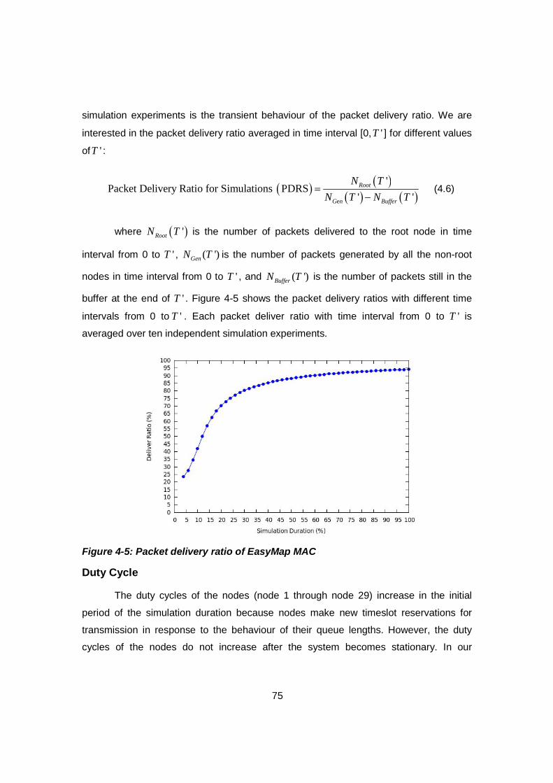
75
simulation experiments is the transient behaviour of the packet delivery ratio. We are
interested in the packet delivery ratio averaged in time interval [0, 'T ] for different values
of 'T :
( ) ( )( ) ( )e
'Packet Delivery Ratio for Simulations PDRS
' 'Root
G n Buffer
N T
N T N T=
- (4.6)
where ( )'RootN T is the number of packets delivered to the root node in time
interval from 0 to 'T , ( ')GenN T is the number of packets generated by all the non-root
nodes in time interval from 0 to 'T , and ( ')BufferN T is the number of packets still in the
buffer at the end of 'T . Figure 4-5 shows the packet delivery ratios with different time
intervals from 0 to 'T . Each packet deliver ratio with time interval from 0 to 'T is
averaged over ten independent simulation experiments.
Figure 4-5: Packet delivery ratio of EasyMap MAC
Duty Cycle
The duty cycles of the nodes (node 1 through node 29) increase in the initial
period of the simulation duration because nodes make new timeslot reservations for
transmission in response to the behaviour of their queue lengths. However, the duty
cycles of the nodes do not increase after the system becomes stationary. In our
76
simulation the system becomes stationary at around 432 seconds of the simulation time.
We present the duty cycles of the nodes after the system becomes stationary.
The duty cycle of EasyMap MAC is the averaged value over ten independent
simulation experiments. For each independent simulation experiment, we recorded the
nodes’ NAs after 432 seconds of the simulation time. Then, according to formula (4.5),
we calculated the duty cycle of each node (node 1 through node 29 in Figure 4-3). We
calculated the duty cycle of each independent simulation experiment by averaging the
duty cycles of the nodes. Finally, we calculated the averaged duty cycle over ten
independent simulation experiments, which is 6.86%. EasyMap MAC can operate with
very low duty cycle, thereby achieving low-energy consumption.
77
5. Conclusion and Future Work
5.1. Conclusions
We designed our own MAC protocol, EasyMap MAC. Two core ideas of
EasyMap are the node ID and the neighborhood map, and with them EasyMap solves
the hidden node problem and achieves very low duty cycle.
EasyMap defines a new format of the superframes. A superframe consists of the
control section and the application section. The control section consists of the control
timeslots, and the application section consists of the application timeslots. Due to this
separation, a control message never collides with an application message, which greatly
diminishes the chance of message collisions. The length of EasyMap control timeslots is
shorter than that of the application timeslots. This differentiation of the timeslot lengths
increases network efficiency and enables the network to decrease the duty cycle. For
the simulation results presented in this thesis, the length of the control timeslots was set
about 10 times shorter than that of the application timeslots. This way, the nodes can
save much of the wakeup time, especially for the dense networks.
We implemented the EasyMap MAC protocol onto NS-2 and compared the
performance of the packet delivery ratio with IEEE 802.15.4. The simulation results
show that EasyMap protocol completely outperforms IEEE 802.15.4 in terms of the
packet delivery ratio in the similar environments. We also tested EasyMap MAC protocol
that employs our timeslot reservation policy. The simulation results show that EasyMap
MAC system becomes stationary in a very early in the simulation duration. The packet
delivery ratio approaches 1 when the simulation ends. In our simulations, the duty cycle
of EasyMap MAC is only about 6.8%. The simulation results indicate that the EasyMap
MAC protocol is a reliable and energy-efficient MAC protocol.
78
5.2. Future Work
Our current simulation only considers an exactly linear physical topology. We do
not know the performance of EasyMap MAC when the physical topology is more
complicated. The collisions might occur more frequently in the dense networks. Thus, to
understand the performances of EasyMap MAC comprehensively, more simulations
based on different topologies are required.
The control timeslot pre-assignment constrains the scalability of the network.
EasyMap MAC protocol tends to work for small or medium wireless sensor networks.
EasyMap MAC protocol might have to be modified for a wireless sensor networks much
larger than the one we simulated.
We defined the first-beacon policy for the joining node in the association
procedure. A better joining policy might be designed to allow the joining node to join the
network more efficiently.
EasyMap MAC is a single-directional transmission protocol. The data flow is
always from the child to the parent. However, sometimes downstream traffic is required,
which is the data packets required to be transmitted by the parent to the child. EasyMap
MAC with the downstream traffic has not been designed yet.

79
References
[1] IEEE Standard 802.15.4-2006, Part 15.4: Wireless Medium Access Control (MAC) and Physical Layer (PHY) Specifications for Low-Rate Wireless Personal Area Networks (WPANs), 2006
[2] V. P. Rao, “The Simulative Investigation of Zigbee/IEEE 802.15.4”, Master Thesis, Dresden University of Technology, Dresden, Germany, 2005.
[3] A. Koubaa, A. Cunha, M. Alves, “A time division beacon scheduling mechanism for IEEE 802.15.4/ZigBee cluster-tree wireless sensor networks,” in Proceedings of 19th Euromicro Conference on Real-Time Systems (ECRTS), 2007.
[4] U. Pešovic, J. Mohorko, K. Benkic, Z. Cucej, “Effect of hidden nodes in IEEE 802.15.4/ZigBee Wireless Sensor Networks”, 17th Telecommunications forum TELFOR, 2009.
[5] G. Anastasi, M. Conti, M. D. Francesco, “A Comprehensive Analysis of the MAC Unreliability Problem in IEEE 802.15. 4 Wireless Sensor Networks," IEEE Transactions on Industrial Informatics, vol. 7, no. 1, pp. 52–65, 2011.
[6] A. Koubaa, M. Alves, E. Tovar, “A Comprehensive Simulation Study of Slotted CSMA/CA for IEEE 802.15.4 Wireless Sensor Networks”, in Proceedings of IEEE Intern-ational Workshop on Factory Communication Systems (WFCS’06), 2006.
[7] B. Nefzi, Y.-Q. Song, A. Koubaa, M. Alves, “Improving the IEEE 802.15.4 Slotted CSMA/CA MAC for Time-Critical Events in Wireless Sensor Networks”, in Proceedings of the 5th International Workshop on Real-Time Networks (RTN’06), 2006.
[8] Bluetooth Special Interest Group (SIG), “Bluetooth Specification Version 4.0 [Vol 0]”, 2010,
[9] Available: http://blog.laptopmag.com/just-what-is-bluetooth-4-0-anyway.
[10] Available: http://www.onworld.com/html/newsresearch.htm
[11] Y. Wei, H. John, E. Deborah, “An Energy-Efficient MAC Protocol for W-ireless Sensor Networks”, in Proceedings of Twenty-First Annual Joint Conference of the IEEE Computer and Communications Societies (INFOCOM), 2002.
[12] T. Dam, K. Langendoen, “An Adaptive Energy-Efficient MAC Protocol for Wireless S-ensor Networks”, in Proceedings of the first ACM Conference on Embedded Networked Sensor Systems (SenSys), 2003.
[13] E. Seyedin, D.C. Lee, S. Yang, E. Lee, D. Boone, M. Steiner-Jovic, “Powermesh medium access control protocol”, in Proceedings of the 5th International Conference on Signal Processing and Communication Systems (ICSPCS), 2011.

80
[14] E. Seyedin, “NapMap Protocol”, Master Thesis, Simon Fraser University, British Columbia, Canada, 2012.
[15] N. Rhee, A. Warrier, M. Aia, “ZMAC: A Hybrid MAC for Wireless Sensor Networks”, in Proceedings of the 3rd ACM Conference on Embedded Networked Sensor Systems, 2005.
[16] J. Polastre, J. Hill, D. Culler, “Versatile low power media access for wireless sensor networks”, in Proceedings of the 2nd international conference on Embedded networked sensor systems, 2004.
[17] Network Simulator NS2. Available: http://www.isu.edu/nsnam/ns
[18] K. Fall, K. Varadhan, “The NS Manual”, VINT Project, 2005.
[19] J. Zheng, M. J. Lee, “A Comprehensive Performance Study of IEEE 802.15.4”, in IEEE Press Book, 2004.
[20] Available: http://en.wikipedia.org/wiki/ZigBee
[21] Available: http://en.wikipedia.org/wiki/Lions_Gate_Bridge

81
Appendices

82
Appendix A.
Recall that IEEE 802.15.4 does not define the beacon period scheduling mechanism for multi-hop topologies. Thus, the linear physical network topology of Figre 4-1 can not be formed thorugh standard IEEE 802.15.4 mechanisms alone. To comapre IEEE 802.15.4 and EasyMap MAC protocl in such linear topology, we proposed a staggered beacon period schediuling mechanism for IEEE 802.15.4. Figure A-1 illustrates the staggered beacon period sheduling for the three nodes of Figure 4-1, Node 1, Node 2, and Node 3. The active periods of the nodes (node 1 through node 8 in Figure 4-1) have the same length (same SO for the nodes), but the active periods of the nodes are not fully overlapping. Similarly, the BIs of the nodes have the same length (same BO for the nodes) as well, and the BIs of the nodes are not fully overlapping. In this mechanism, a node, say node 1, not only wakes up during its active period, but also wakes up at its parent’s (node 0’s) beacon timeslot for receiving node 0’s beacon. When a node is joining the network, the joining node can only receive one node’s beacon within its radio range in the physical topology in Figure 4-1. For example, when Node 1 is joining the network, it only receives the beacon from Node 0. After Node 1 joins the network, Node 0 becomes Node 1’s parent. Then, Node 1 broadcasts its beacon right after receving the beacon of Node 0. Node 1 broadcasts its beacon at Node 1’s beacon timeslot after it joins the network. Node 0 receives Node 1’s beacon and simply discards it because the parent does not receive the child’s beacon in this mechanism. Similarly, when Node 2 is joining the network, Node 2 only receives the beacon of Node 1. After Node 2 joins the network, Node 2 broadcasts its beacon right after receiving Node 1’s beacon. This way, the linear network topology of Figure 4-1 can be formed in a wireless network of IEEE 802.15.4 with the staggered beacon scheduling mechanism.
Node 0’s beacon timeslot Node 1’s beacon timeslot
Node 2’s beacon timeslot Node 3’s beacon timeslot
Figure A-1: Staggered Beacon Period Scheduling Mechanism
83
Appendix B.
Nodes’ buffers are empty at the beginning of the simulations, and thus the packets generated in the early part of the simulation have lower probability to be dropped due to buffer overflow. To present more accurate simulation results, we discard the initial transient period of the simulation duration for analyzing the simulation results. The packet drop ratios can guide us as to know when we consider the system has reached steady state.
We define an empirical packet drop ratio averaged over interval [0, ''T ] from a simulation as:
( ) ( )( ) ( )
''PDRRS ''
'' ''Drop
Gen Buffer
N TT
N T N T=
- (B.1)
( )''DropN T is the number of packet drops due to buffer overflow in time interval from 0 to ''T .
( '')GenN T is the number of packets generated by all the non-root nodes (node 1 through node 8
in Figure 4-1) in time interval from 0 to ''T . ( '')BufferN T is the number of packets generated in
the time interval from 0 to ''T but still in the buffer at time ''T .The packet drop ratio,
( )PDRRS ''T is relatively low in the early part of the simulation duration (i.e., for small ''T )
because of the initially empty buffers. As the simulation time goes on, the packet drop ratio keeps increasing, and it eventually becomes almost steady. For example, Figure B-1 shows the packet drop ratio plotted against ''T for the traffic load of 0.9 packet/second in IEEE 802.15.4.
To have an accurate estimation of formula (4.1), we avoid taking into account the packet behaviours in what we consider the transient period, which is the interval of time before the packet drop ratio is considered to have reached a plateau. We denote PT as the time at which
the packet drop ratio is considered to have reached a plateau. From the graph of the packet drop ratio plotted against ''T , we can choose a value of PT . We only use the period after PT for
calculating the packet delivery ratio. We will refer to this as Adjusted Packet Delivery Ratio (APDR), and the mathematical formula for this is
Adjusted Packet Delivery Ratio, (APDR) = ( ) ( )( ) ( ) ( ) ( )en ( )
Root Root P
G Gen P Buffer Buffer P
N T N T
N T N T N T N T
-- - -
(B.2)
where ( )Root PN T is the number of packets delivered to the root node in time interval from 0 to
PT , ( )enG PN T is the number of packets generated by the non-root nodes in time interval from 0
to PT . ( )Buffer PN T is the number of packets generated by the non-root nodes in time interval from
0 to PT but still in the buffer when simulation ends.
We note that PT can be different for different traffic loads, and even for the same traffic load,
PT can be different in different protocols. For EasyMap MAC protocol, we did not see any packet
drop for all the seven traffic loads in the first set of simulations − that is, the packet drop ratio is 0
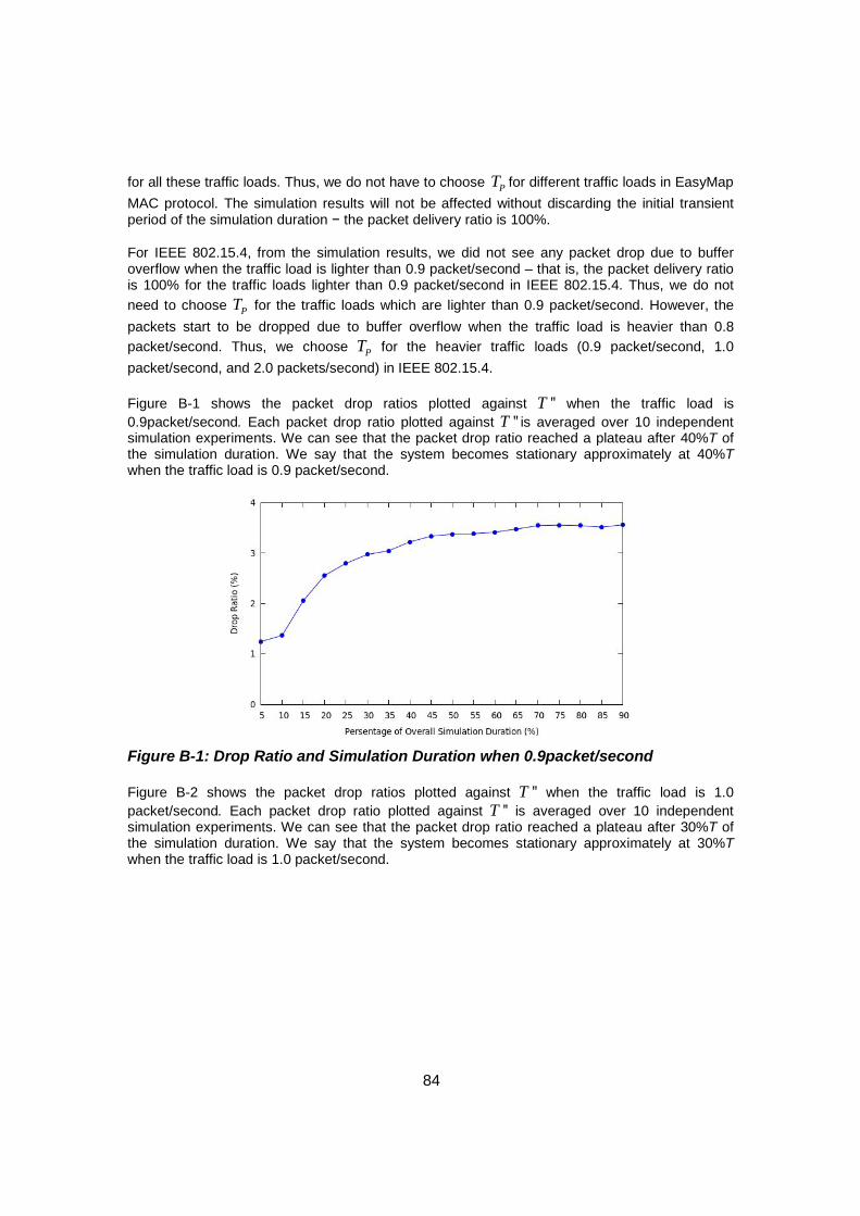
84
for all these traffic loads. Thus, we do not have to choose PT for different traffic loads in EasyMap
MAC protocol. The simulation results will not be affected without discarding the initial transient period of the simulation duration − the packet delivery ratio is 100%.
For IEEE 802.15.4, from the simulation results, we did not see any packet drop due to buffer overflow when the traffic load is lighter than 0.9 packet/second – that is, the packet delivery ratio is 100% for the traffic loads lighter than 0.9 packet/second in IEEE 802.15.4. Thus, we do not need to choose PT for the traffic loads which are lighter than 0.9 packet/second. However, the
packets start to be dropped due to buffer overflow when the traffic load is heavier than 0.8 packet/second. Thus, we choose PT for the heavier traffic loads (0.9 packet/second, 1.0
packet/second, and 2.0 packets/second) in IEEE 802.15.4.
Figure B-1 shows the packet drop ratios plotted against ''T when the traffic load is 0.9packet/second. Each packet drop ratio plotted against ''T is averaged over 10 independent simulation experiments. We can see that the packet drop ratio reached a plateau after 40%T of the simulation duration. We say that the system becomes stationary approximately at 40%T when the traffic load is 0.9 packet/second.
Figure B-1: Drop Ratio and Simulation Duration when 0.9packet/second
Figure B-2 shows the packet drop ratios plotted against ''T when the traffic load is 1.0 packet/second. Each packet drop ratio plotted against ''T is averaged over 10 independent simulation experiments. We can see that the packet drop ratio reached a plateau after 30%T of the simulation duration. We say that the system becomes stationary approximately at 30%T when the traffic load is 1.0 packet/second.
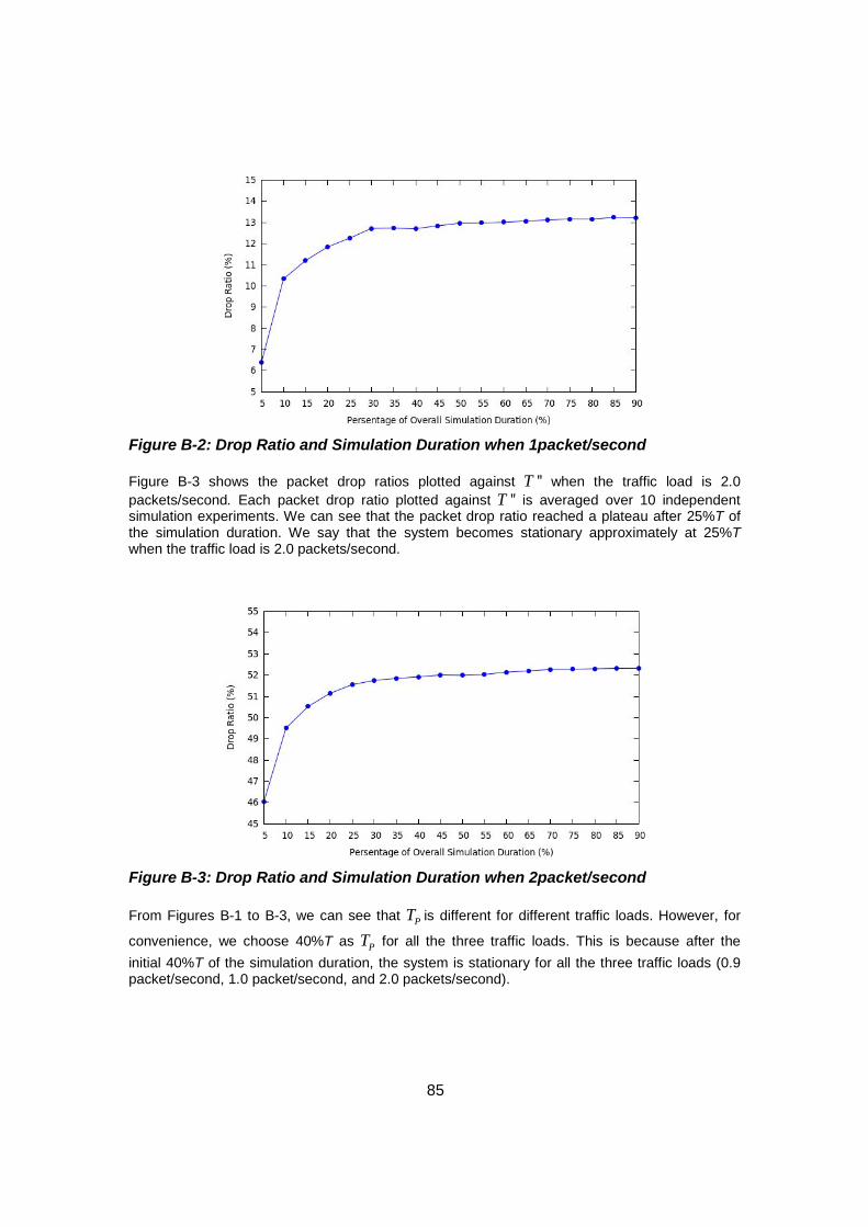
85
Figure B-2: Drop Ratio and Simulation Duration when 1packet/second
Figure B-3 shows the packet drop ratios plotted against ''T when the traffic load is 2.0 packets/second. Each packet drop ratio plotted against ''T is averaged over 10 independent simulation experiments. We can see that the packet drop ratio reached a plateau after 25%T of the simulation duration. We say that the system becomes stationary approximately at 25%T when the traffic load is 2.0 packets/second.
Figure B-3: Drop Ratio and Simulation Duration when 2packet/second
From Figures B-1 to B-3, we can see that PT is different for different traffic loads. However, for
convenience, we choose 40%T as PT for all the three traffic loads. This is because after the
initial 40%T of the simulation duration, the system is stationary for all the three traffic loads (0.9 packet/second, 1.0 packet/second, and 2.0 packets/second).


