

Emission Rates of Intermodal Rail/Road and Road-onlyTransportation in Europe: A Comprehensive Simulation Study
Arne Heinold∗, Frank MeiselSchool of Economics and Business, Kiel University, Kiel, Germany
Abstract
Intermodal rail/road transportation combines advantages of both modes of transport and is often
seen as an effective approach for reducing the environmental impact of freight transportation. This
is because it is often expected that rail transportation emits less greenhouse gases than road trans-
portation. However, the actual emissions of both modes of transport depend on various factors
like vehicle type, traction type, fuel emission factors, payload utilization, slope profile or traffic
conditions. Still, comprehensive experimental results for estimating emission rates from heavy
and voluminous goods in large-scale transportation systems are hardly available so far. This study
describes an intermodal rail/road network model that covers the majority of European countries.
Using this network model, we estimate emission rates with a mesoscopic model within and be-
tween the considered countries by conducting a large scale simulation of road-only transports and
intermodal transports. We show that there are high variations of emission rates for both road-only
transportation and intermodal rail/road transportation over the different transport relations in Eu-
rope. We found that intermodal routing is more eco-friendly than road-only routing for more than
90% of the simulated shipments. Again, this value varies strongly among country pairs.
Keywords: emission rates, european rail/road network, intermodal transportation, simulation,
mesoscopic model
∗Corresponding author.Email addresses: [email protected] (Arne Heinold), [email protected]
(Frank Meisel)
September 5, 2018

1. Introduction
In 2015, a total of 4,452 million tons of anthropogenic CO2 equivalent greenhouse gases were
emitted in the European Union (EU), see Eurostat (2018b). Around 20% of these emissions re-
sulted from transportation (Eurostat, 2018b), where road transportation is the dominant mode in
the freight sector. For example, 75.3% of the total inland freight ton-kilometers (ton-km) in the
EU were transported by truck, 18.3% by train and 6.4% by inland waterways in 2015 (Eurostat,
2018a). Recent research and political initiatives that seek for a reduction of the human-made en-
vironmental impact therefore also focus on emissions from transportation, see e.g. McKinnon
et al. (2012), Psaraftis and Kontovas (2016), or DIN EN 16258 (2012). The amount of greenhouse
gases (GHG) emitted per ton-km are used as a typical measure for the environmental impact of
freight transportation. Although greenhouse gases subsume various substances like carbon diox-
ide, methane, nitrous oxide, hydrofluorocarbons, perfluorocarbons and sulphur hexafluoride, their
global warming potential can be expressed as carbon dioxide equivalents (CO2e) and, therefore,
the amount of CO2e per ton-km is considered a valid indicator of the environmental performance
of freight transportation. Shifting freight from road to rail is often seen as an effective option to
improve this measure (e.g. Dekker et al., 2012, McKinnon et al., 2012). Thereby, an objective
comparison of transport options requires to consider well-to-wheel emissions that include not just
the actual emissions of the transport operation (so called tank-to-wheel emissions) but also the
emissions caused by producing and providing the fuel or energy to the vehicle (so called well-to-
tank emissions), see Hoffrichter et al. (2012), Moro and Lonza (2017).
Research in the field of environmental transportation focusses on the development of eco-
oriented routing and transport flow models (e.g. Bauer et al., 2010; Behnke and Kirschstein, 2017;
Bektas and Laporte, 2011; Ehmke et al., 2016; Rudi et al., 2016). Such studies usually consider
emission rates obtained from emission estimation models or they use aggregated empirical rates
reported in the literature. Experimental results in such papers typically refer to artificial networks
or to relatively small real networks that cover a specific region. A comprehensive overview of
emission rates that are observed in large-scale transportation systems like the European rail/road
system is not provided by these studies. With our paper, we fill this gap and provide a systematic
2

and broad overview of emission rates from intermodal rail/road and road-only transportation in
Europe. More precisely, we analyze intra- and inter-country freight shipments for 27 European
countries. We conduct a comprehensive simulation study that respects country specific attributes
like the electrification and density of the rail network and geographical characteristics. To this end,
we (i) collect data of an intermodal rail network across the considered countries, based on the cor-
ridors from the Trans-European Transport Network policy (TEN-T), see European Commission
(2018), (ii) adapt a suitable emission estimation model for rail and road transportation and (iii)
present results from an extensive simulation study that covers numerous experimental settings.
We focus on relatively large shipments of several truck loads of heavy and voluminous goods, as
these are candidates for rail transportation. Next to the differentiation between heavy and volumi-
nous goods, we analyze the impact of further vehicle characteristics, shipment characteristics, and
route characteristics such as traction type, electric emission factors, cargo size, gradient or traffic
conditions. To estimate emissions, we adapt the mesoscopic model from Kirschstein and Meisel
(2015). This model can capture both road and rail transportation and allows us to test the relevance
of the previously mentioned parameters for the European transport system. We also contribute to
the improvement of this estimation model by presenting an alternative way of approximating the
gradient of a route. With these contributions, we present a broad and holistic overview of inter-
modal rail/road emission rates for European countries. The results of this study can be used to
further facilitate research in areas where emission rates serve as an input to environmentally ori-
ented decision problems, such as location planning or routing problems. They might also be used
for companies to benchmark their environmental performance. In addition, the derived model of
the European rail and road network can be used for follow-up research in the field of intermodal
transportation.
The paper is organized as follows. Section 2 formally describes the intermodal rail/road net-
work and the used data. Section 3 briefly reviews literature on emission estimation models and
provides details about the mesoscopic estimation model. Section 4 describes the simulation set-
tings and Section 5 presents the obtained results. Section 6 concludes this paper. The paper is
supplemented by an extensive appendix that provides look-up tables for emission rates of road,
rail and intermodal rail/road transportation for all country combinations and simulation settings
3

considered in this study.
2. Modelling the European Rail/Road Network
2.1. Multilayer Network Structure for Intermodal Transportation
Intermodal networks can be formally modelled as multilayer networks (e.g. Southworth and
Peterson, 2000). An example of such network models is the Geospatial Intermodal Freight Trans-
portation (GIFT) model for the United States that is also implemented as a web-tool (WebGIFT,
2018). This model covers various modes (rail, road, water) and enables the exploration of tradeoffs
between cost, time and environmental measures. A description of the model and case studies can
be found in Hawker et al. (2010), Winebrake et al. (2008) and Comer et al. (2010). For our study,
we define here a rail/road network G(N , E), where nodes N = N rail ∪ N trans ∪ N road ∪ N cust
and edges E ⊂ N × N form four interconnected layers with subgraphs Grail, Gtrans, Groad and
Gcust, see Figure 1. Nodes on these four layers are: (i) customer nodes N cust that are origins and
destinations of shipments, (ii) nodes N road that belong to the road layer, (iii) nodes N trans that
enable freight transshipment between the road and rail mode, and (iv) nodes N rail that belong to
the rail layer.
(a) road-only routing as solid lines
1
2 6
3
45
7 10 13 14
19
9
23
8
1615
25
20
2421
22
17 18
11
12
G𝑟𝑎𝑖𝑙
G𝑡𝑟𝑎𝑛𝑠
G𝑟𝑜𝑎𝑑
G𝑐𝑢𝑠𝑡
(b) intermodal routing as solid lines
1
2 6
3
45
7 10 13 14
19
9
23
8
1615
25
20
2421
22
17 18
11
12
G𝑟𝑎𝑖𝑙
G𝑡𝑟𝑎𝑛𝑠
G𝑟𝑜𝑎𝑑
G𝑐𝑢𝑠𝑡
Figure 1: Exemplary routings through an intermodal multilayer network.
The railway network Grail(N rail, Erail) within the uppermost layer is an incomplete network
described by nodes N rail (nodes 19 to 25 in the example) and edge set Erail ⊂ N rail ×N rail. The4

transshipment network Gtrans(N trans, E trans) represents the operational transshipment processes
and consists of nodes N trans (nodes 17 and 18 in the example) and an empty set E trans = ∅
as there are no edges between transshipment nodes. The road network Groad(N road, Eroad) is an
incomplete network described by nodes N road (nodes 7 to 16 in the example) and edge set Eroad ⊂
N road × N road. The bottom layer states the customer network Gcust(N cust, Eroad) and consists of
all customer nodes N cust (nodes 1 to 6 in the example) and an empty set Eroad as customers
are only connected with each other via the road network. The additional cross-layer edge sets
E trans−rail ⊂ N rail × N trans , E trans−road ⊂ N trans × N road and Ecust−road ⊂ N cust × N road
connect subgraphs Grail, Gtrans, Groad and Gcust. Railway nodes that qualify for transshipment to
the road mode (nodes 19 and 23 in the example) are linked via dedicated transshipment nodes
(nodes 17 and 18 in the example) to dedicated road nodes (nodes 9 and 16 in the example). Note
that each node in N rail and N road is linked to at most one node in N trans and that each node in
N cust is linked to exactly one node in N road.
We denote by (i, j) ∈ E the edge that connects node i ∈ N and node j ∈ N . We consider
asymmetric edge weights because edge characteristics (like gradient iα and distance d introduced
later in Section 3) might differ between edges (i, j) ∈ E and (j, i) ∈ E in a real-world infrastruc-
ture network. Eventually, shipments from an origin i ∈ N cust to a destination j ∈ N cust may use
a road-only routing (Figure 1a) or an intermodal routing (Figure 1b). The road-only routing uses
merely the two bottom layers whereas the intermodal routing uses all four layers. In other words,
we assume that customers do not have direct access to the rail network, although this could be
included in the model without difficulty.
2.2. Network Data for the European Rail and Road Network
We instantiate the theoretical network model from Section 2.1 to represent the rail/road net-
work of the current EU member states, excluding the island states Cyprus, Ireland and Malta but
including the non-EU member states Norway and Switzerland.
The railway network Grail orients along the core corridors of the TEN-T policy. The use of
TEN-T core corridors comes for several reasons: (i) the corridors define all relevant infrastructural
elements, (ii) they also define rail line specific restrictions (e.g. a lack of electrification) and (iii)
5

it can be assumed that all core corridors are relevant for intermodal freight transportation. The set
of railway nodes N rail is derived from respective terminals in the TENtec Interactive Map (2018).
All these nodes qualify for rail/road transshipment. TEN-T contains at most one terminal for most
of the cities. For cities with more than one terminal, we included only the most central one in
our network. This results for example in 14 transshipments nodes for Spain and 4 transshipment
nodes for Austria, see Table 1. Concerning railway edges Erail, we only consider existing tracks as
country transshipment rail line emission customercountry code nodes electrified not electrified coefficient nodes
[-] [-] [km] [km] [gCO2e/kWh] [-]
Austria AUT 4 1,103 66 322 226Belgium BEL 7 838 0 261 83Bulgaria BGR 4 1,114 0 618 297Croatia HRV 2 378 0 487 153Czech Republic CZE 6 1,216 75 657 212Denmark DNK 2 343 121 364 116Estonia EST 1 56 216 878 116Finland FIN 5 520 0 207 384France FRA 16 4,513 0 100 1,500Germany DEU 26 5,176 524 599 956Greece GRC 2 435 408 732 353Hungary HUN 2 1,276 0 383 248Italy ITA 22 3,919 0 413 806Latvia LVA 2 45 374 1,110 170Lithuania LTU 3 95 493 370 172Luxembourg LUX 1 40 0 508 7Netherlands NLD 9 585 0 555 92Norway NOR 1 169 0 9 528Poland POL 9 3,686 100 937 839Portugal PRT 5 1,064 0 372 251Romania ROU 9 1,494 112 449 630Slovakia SVK 2 663 0 412 132Slovenia SVN 2 397 109 309 55Spain ESP 14 3,911 1,349 321 1,370Sweden SWE 5 1,374 0 45 661Switzerland CHE 1 509 0 29 108United Kingdom GBR 9 1,227 494 593 663∑
171 36,147 4,439 11,128
Table 1: Descriptive network data for 27 European countries.
derived from Raildar (2018). We supplement the rail network by auxiliary nodes that split some of
the edges into two or more parts. This is to represent different edge characteristics, such as traction
type or country borders. To increase the network connectivity, we include the projected ’Tallinn-6
Helsinki Tunnel’ between Helsinki (Finland) and Tallinn (Estonia), the planned ’Fehmarn Belt
Tunnel’ between Puttgarden (Germany) and Rødby (Denmark), the train ferry that connects Sicily
with mainland Italy and the train ferry that connects Rostock (Germany) with Trelleborg (Sweden),
see European Parliament (2017), European Commission (2015), BluFerries (2018) and StenaLine
(2018). The traction type of the locomotive on each railway track (either diesel or electric) is
derived from information of the TEN-T Compliance Maps (2014). In total, Grail includes 40,586
kilometers of rail tracks, of which 36,147 kilometers are electrified (89%) and 4,439 kilometers
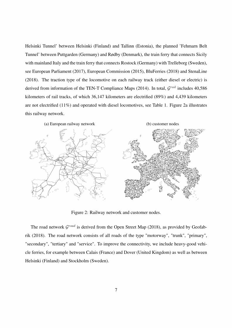
are not electrified (11%) and operated with diesel locomotives, see Table 1. Figure 2a illustrates
this railway network.
(a) European railway network (b) customer nodes
Figure 2: Railway network and customer nodes.
The road network Groad is derived from the Open Street Map (2018), as provided by Geofab-
rik (2018). The road network consists of all roads of the type "motorway", "trunk", "primary",
"secondary", "tertiary" and "service". To improve the connectivity, we include heavy-good vehi-
cle ferries, for example between Calais (France) and Dover (United Kingdom) as well as between
Helsinki (Finland) and Stockholm (Sweden).
7
3. Emission Estimation for Road and Rail Transportation
3.1. Literature Review
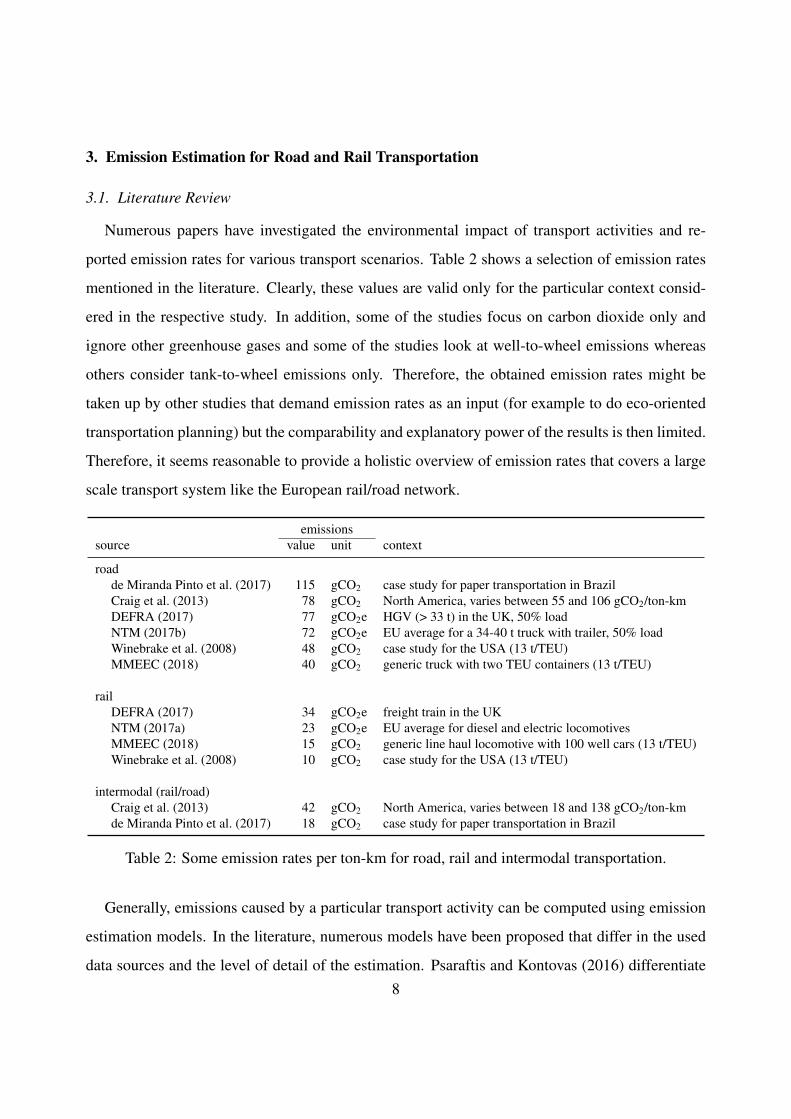
Numerous papers have investigated the environmental impact of transport activities and re-
ported emission rates for various transport scenarios. Table 2 shows a selection of emission rates
mentioned in the literature. Clearly, these values are valid only for the particular context consid-
ered in the respective study. In addition, some of the studies focus on carbon dioxide only and
ignore other greenhouse gases and some of the studies look at well-to-wheel emissions whereas
others consider tank-to-wheel emissions only. Therefore, the obtained emission rates might be
taken up by other studies that demand emission rates as an input (for example to do eco-oriented
transportation planning) but the comparability and explanatory power of the results is then limited.
Therefore, it seems reasonable to provide a holistic overview of emission rates that covers a large
scale transport system like the European rail/road network.
emissionssource value unit context
roadde Miranda Pinto et al. (2017) 115 gCO2 case study for paper transportation in BrazilCraig et al. (2013) 78 gCO2 North America, varies between 55 and 106 gCO2/ton-kmDEFRA (2017) 77 gCO2e HGV (> 33 t) in the UK, 50% loadNTM (2017b) 72 gCO2e EU average for a 34-40 t truck with trailer, 50% loadWinebrake et al. (2008) 48 gCO2 case study for the USA (13 t/TEU)MMEEC (2018) 40 gCO2 generic truck with two TEU containers (13 t/TEU)
railDEFRA (2017) 34 gCO2e freight train in the UKNTM (2017a) 23 gCO2e EU average for diesel and electric locomotivesMMEEC (2018) 15 gCO2 generic line haul locomotive with 100 well cars (13 t/TEU)Winebrake et al. (2008) 10 gCO2 case study for the USA (13 t/TEU)
intermodal (rail/road)Craig et al. (2013) 42 gCO2 North America, varies between 18 and 138 gCO2/ton-kmde Miranda Pinto et al. (2017) 18 gCO2 case study for paper transportation in Brazil
Table 2: Some emission rates per ton-km for road, rail and intermodal transportation.
Generally, emissions caused by a particular transport activity can be computed using emission
estimation models. In the literature, numerous models have been proposed that differ in the used
data sources and the level of detail of the estimation. Psaraftis and Kontovas (2016) differentiate8

between top-down (or fuel-based) and bottom-up (or activity-based) methods. Top-down methods
use the actual fuel consumption or estimate the fuel consumption of an already conducted trans-
port. Emission factors for the respective fuel type are then used to quantify the GHG emissions.
In contrast, bottom-up methods exploit relevant parameters of the transport activity (used vehi-
cle type, distance, etc.) and estimate emissions with the help of look-up values. Another way to
classify emission models is to differentiate between microscopic and macroscopic models (Scora
and Barth, 2006). Microscopic models estimate emissions as precisely as possible by considering
detailed physics of the moving vehicle, such as air resistance and rolling resistance. Macroscopic
models are less precise and use, similar to bottom-up methods, empirical data to estimate emis-
sions. Macroscopic models usually combine trip specific information, such as road profile and
average speed, with vehicle specific information, such as tare weight and fuel type.
A large number of emission estimation models is designed either for road or for rail freight
transportation. An overview of models for road transportation is provided by Demir et al. (2011).
A popular model in this field is the Comprehensive Modal Emissions Model (CMEM) from Scora
and Barth (2006). A popular model for rail transportation is the ARTEMIS (Assessment and Relia-
bility of Transport Emission Models and Inventory Systems) model from Lindgreen and Sorenson
(2005b). Both models follow the microscopic idea and derive emissions from a very detailed es-
timation of fuel or energy demands. Emission estimation models that cover both road and rail
transportation often follow a macroscopic approach. The EcoTransIT World Initiative (2016) de-
veloped the EcoTransIT model that covers all major transportation modes (road, rail, water, air).
Another macroscopic model for road and rail is the MEET (Methodologies for Estimating Air Pol-
lutant Emissions from Transport) model from Hickman et al. (1999). The authors derive emission
functions and parameters from real-world experiments for various vehicle types. Kirschstein and
Meisel (2015) propose a mesoscopic model for road and rail transportation that combines the most
relevant factors from microscopic models with empirical data from macroscopic models. The au-
thors follow the physical base model from Ross (1997), which derives the required energy from
factors like speed, weight, grade or acceleration. The relevance of these factors has been discussed
in several other studies, such as Hickman et al. (1999) or Stead (1999). From the energy demand,
the mesoscopic model deducts the amount of emitted greenhouse gases through emission factors.
9

This procedure is similar to other emission estimation models, such as the model from DeLuchi
(1991) or the GREET model from Wang (1999). Like Hickman et al. (1999) and others, the
mesoscopic model supports trip specific acceleration profiles and thus allows for a consideration
of various traffic conditions, like urban traffic and highway traffic. Kirschstein and Meisel (2015)
show that this differentiation can have a significant impact on emission rates. Like all other models
that cover road and rail, also the mesoscopic model can be used for an environmental assessment
of intermodal rail/road transports. For the purpose of our study, the mesoscopic model describes a
good trade-off between the required input data and the accuracy of estimated emissions. The next
two subsections describe the methodology of the mesoscopic model for road transportation and
for rail transportation.
3.2. Estimating Emissions from Road Transportation
The mesoscopic model derives emissions for road transportation by estimating the fuel demand
of a transport operation. Equation (1) represents the main formula for computing GHG emissions
and Table 3 shows the adopted notation. The formula first estimates the energy demand Wtruck
for moving the truck, taking into account the distance d of a considered trip, the gradient i of the
route, the total weight m (including payload mpayload and tare weight mtare), the average number of
acceleration processes per kilometer nacc and the average speed v of the expected traffic conditions.
For details of the corresponding computation, we refer to Kirschstein and Meisel (2015).
GHGtruck =(
Wtruck(d, i, m, nacc, v) · rfull − ridle
εt(v) · pvehicle+ ridle · d
v
)· k (1)
Formula (1) weights Wtruck to convert the energy demand into a fuel demand by taking into
account the transmission efficiency of the truck εt(v), which depends on the average speed v, the
maximal power of the engine pvehicle and the fuel consumption rate if the truck is idle ridle or at full
power rfull. The calculation requires further truck and fuel type specific parameters, namely the
front surface A of the truck, the air resistance coefficient cair, the rolling resistance coefficient croll
and the energy coefficient p for diesel fuel. Corresponding values are also listed in Table 3. All
values belong to a 40 t diesel truck, which is the vehicle type considered for road transportation
throughout our study. Eventually, Formula (1) multiplies the fuel demand with a well-to-wheel10

notation value unit description
trip specificWtruck
∗ kWh required energy to move the truckd ∗ km distancei ∗ % gradientm ∗ t total weightmpayload ∗ t payloadnacc ∗ - average number of accelerations per kmv ∗ km/h average speed
truck and fuel type specificmtare 14 t tare weight of the truckεt(v) ~0.88 - transmission efficiencypvehicle 300 kW maximal power of the engineridle 3 l/h fuel consumption rate if truck is idlerfull 68.7 l/h fuel consumption rate if truck is at full powerA 9 m2 front surface area of the truckcair 0.6 - air resistance coefficientcroll 0.006 - rolling resistance coefficientp 0.0811 l/kWh well-to-wheel energy coefficient (diesel)k 3.15 kgCO2e/l well-to-wheel emission coefficient (diesel)
∗ computed from other parameters or varied in the simulation
Table 3: Notation of the mesoscopic model for road transportation.
emission coefficient k to convert the amount of diesel into an amount of CO2e.
One of the parameters that needs to be provided to the mesoscopic model is the gradient i of
the route. This gradient is then used to calculate the power to overcome the difference in altitude,
which becomes part of the total energy to move the truck Wtruck. For a path that connects some
origin location with some destination location, an intuitive way to calculate this gradient i is to
compare the altitude of the origin with the altitude of the destination. However, this approach can
result in the same gradient value for two paths with very different slope profiles, see Figure 3. The
path from A to B in Figure 3a goes through a hilly terrain with partially steep gradients whereas
the path from C to D in Figure 3b goes through a terrain with a modest but constant gradient.
Since the altitude of origins A and C, the altitude of destinations B and D and the distance d =
50 km are identical, the simple origin-destination altitude difference leads to the same gradient for
both routes and, thus, presumes an identical energy demand for both routes.
11

(a) terrain with a volatile slope profile
Alpha gradient (in %)
0 1.100
0.1 1.040
0.2 0.980
0.3 0.920
0.4 0.860
0.5 0.800
0.6 0.740
0.7 0.680
0.8 0.620
0.9 0.560
1 0.500
EXPORT SEITE 5 (path a)
0
50
100
150
200
250
300
350
hei
ght
[m]
distance [km]
z1 z2 z3 z4 z50
A
50
B
(b) terrain with a constant slope profile
Alpha gradient (in %)
0 0.500
0.1 0.500
0.2 0.500
0.3 0.500
0.4 0.500
0.5 0.500
0.6 0.500
0.7 0.500
0.8 0.500
0.9 0.500
1 0.500
EXPORT SEITE 7 (path b)
0
50
100
150
200
250
300
350
hei
ght
[m]
distance [km]
z1 z2 z3 z4 z50
C
50
D
Figure 3: Two routes with different slope profiles.
To resolve this issue, we introduce the concept of the adjusted gradient iα, where we differen-
tiate between positive and negative slopes. For this, we split the path, which is of total distance d,
into n equally sized segments. We refer to the ith segment as zi and denote by alt(z1i ) the altitude
of the starting point of segment zi and by alt(z2i ) the altitude of the ending point of segment zi.
Furthermore, we compute by uzi= max{alt(z2
i ) − alt(z1i ), 0} the positive altitude difference in
segment zi and by vzi= max{alt(z1
i ) − alt(z2i ), 0} the negative altitude difference in segment zi.
The calculation of the adjusted gradient iα is shown in Formula (2) where 0 ≤ α ≤ 1 is a preset
weight.
iα = 1d
·∑zi
(uzi− α · vzi
) (2)
The idea behind iα is to fully account for positive slopes (uzi) and to (partially) subtract negative
slopes (vzi). Note that negative slopes reduce the energy required to overcome other physical
forces, such as rolling resistance or air resistance, and thus reduces the total energy demand (Ross,
1997). In addition, new technologies enable energy recoveries from negative slopes, such as the
deceleration energy of trains. However, the original gradient i assumes that energy from negative
slopes can be recovered totally. This might even lead to situations where energy recovered from
negative slopes exceeds all other energy demands and results in a negative overall energy demand,
which is definitely unrealistic. With the introduction of α we can control to what extent this energy
is recovered. In case α = 0 only positive slopes are considered for the calculation of the adjusted
gradient and downhill segments are treated like segments with flat terrain. In other words, α = 0
means that no energy is recovered from negative slopes at all. With a value of α > 0 energy from
12

negative slopes is partially recovered. The extreme case of α = 1 represents a full recovery of
energy from negative slopes, identical to the original gradient i. In Table 4 we show iα for the
examples from Figure 3 and for α ∈ [0, 0.2, . . . , 1]. The adjusted gradient in Figure 3a increases
with lower values of α, because the negative slopes are gradually ignored. For the reversed path
that goes from B to A this leads to a change in the sign of iα. In Figure 3b, no segment of the
path going from C to D has a negative altitude difference (vzi= 0, ∀ i = 1, . . . , n), which makes
iα independent of the value of α. Respectively, for the reversed path that goes from D to C, all
segments have a negative altitude difference (vzi> 0, ∀ i = 1, . . . , n) and iα decreases with higher
values of α.
Figure 3a Figure 3b
α A → B B → A C → D D → C
0.0 1.10 0.60 0.50 0.000.2 0.98 0.38 0.50 -0.100.4 0.86 0.16 0.50 -0.200.6 0.74 -0.06 0.50 -0.300.8 0.62 -0.28 0.50 -0.401.0 0.50 -0.50 0.50 -0.50
Table 4: Adjusted gradients iα (in %) for the paths from Figure 3.
3.3. Estimating Emissions from Rail Transportation
For rail freight transportation, the mesoscopic model differentiates between diesel and electric
trains. Still, the main idea for both types of power supply is to estimate the energy demand Wtrain
for moving the train and, then, either directly derive the emissions from this amount of energy
(electric train) or use an energy coefficient p to first convert the energy demand into a fuel demand
(diesel train). Formula (3) shows the calculation that is common for both types of power supply.
Table 5 lists the corresponding notation.
GHGtrain = Wtrain(d, i, m, ncar, nacc, v)ε
· p · k (3)
The energy demand Wtrain is computed from distance d, gradient i, total weight m, number of
rail cars ncar, number of accelerations per kilometer nacc and average speed v. Here d, i, nacc and v
13
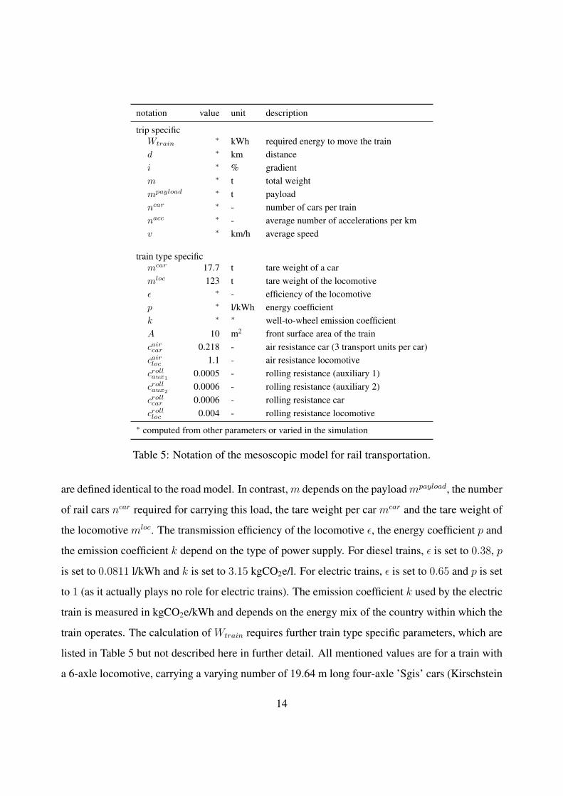
notation value unit description
trip specificWtrain
∗ kWh required energy to move the traind ∗ km distancei ∗ % gradientm ∗ t total weightmpayload ∗ t payloadncar ∗ - number of cars per trainnacc ∗ - average number of accelerations per kmv ∗ km/h average speed
train type specificmcar 17.7 t tare weight of a carmloc 123 t tare weight of the locomotiveε ∗ - efficiency of the locomotivep ∗ l/kWh energy coefficientk ∗ ∗ well-to-wheel emission coefficientA 10 m2 front surface area of the traincair
car 0.218 - air resistance car (3 transport units per car)cair
loc 1.1 - air resistance locomotivecroll
aux10.0005 - rolling resistance (auxiliary 1)
crollaux2
0.0006 - rolling resistance (auxiliary 2)croll
car 0.0006 - rolling resistance carcroll
loc 0.004 - rolling resistance locomotive∗ computed from other parameters or varied in the simulation
Table 5: Notation of the mesoscopic model for rail transportation.
are defined identical to the road model. In contrast, m depends on the payload mpayload, the number
of rail cars ncar required for carrying this load, the tare weight per car mcar and the tare weight of
the locomotive mloc. The transmission efficiency of the locomotive ε, the energy coefficient p and
the emission coefficient k depend on the type of power supply. For diesel trains, ε is set to 0.38, p
is set to 0.0811 l/kWh and k is set to 3.15 kgCO2e/l. For electric trains, ε is set to 0.65 and p is set
to 1 (as it actually plays no role for electric trains). The emission coefficient k used by the electric
train is measured in kgCO2e/kWh and depends on the energy mix of the country within which the
train operates. The calculation of Wtrain requires further train type specific parameters, which are
listed in Table 5 but not described here in further detail. All mentioned values are for a train with
a 6-axle locomotive, carrying a varying number of 19.64 m long four-axle ’Sgis’ cars (Kirschstein
14

and Meisel, 2015, Lindgreen and Sorenson, 2005a,b). These cars can carry at most three 20-foot
containers or a total of 62 tons.
4. Simulation Settings
Our simulation study aims at estimating emission rates for shipments within and between the
considered European countries. Section 4.1 describes the creation of shipments and their routing in
the network. Section 4.2 describes the specification of trip specific parameters for the mesoscopic
model and derives an appropriate number of shipments to simulate per country pair. Finally,
Section 4.3 describes different configurations that are later explored by experiments in Section 5.
4.1. Generation of Shipments and Routing
We generate shipments within and between 27 European countries. We denote by C the set
of these countries. Given a country pair (c1, c2), with c1 ∈ C and c2 ∈ C, we generate a set of
shipments Sc1,c2 for this transport relation. In case of c1 = c2 these shipments have their origin
and destination in the same country whereas in case of c1 6= c2 shipments have their origin and
destination in different countries.
Each shipment s ∈ Sc1,c2 is defined by its payload ls (in tons), its origin location os and its
destination location ds. For the payload ls, we first draw a random shipment size ts ∈ [6, 7, . . . , 24]
of transport units (TU). Each such unit corresponds to a 20-ft equivalent container unit or a similar
load device. Accordingly, the lowest shipment size of 6 transport units refers to 3 full truck loads
or 2 full rail cars whereas the largest shipment size of 24 transport units refers to 12 full trucks or 8
full rail cars. We then assume a gross weight of 11 t per transport unit for heavy goods and 6 t per
transport unit for voluminous goods, which leads to the payload ls of shipment s. For the origin
os and the destination ds, we first preprocess a set of candidate customer node N custi per country
i ∈ C, with N cust = ⋃i∈C N cust
i . Node locations are drawn uniformly from latitude/longitude
values that belong to the country, where we exclude locations that are not connected to the road
network Groad (for example small islands). The number of candidate locations per country is
proportional to the land area of this country. For France, which is the largest country in C, we
draw 1,500 random locations. For each other country, the number of candidate locations derives
15

from its land area in comparison to France. For example, the land area of Latvia is 11.3% of the
area of France and we thus generate 170 customer nodes in Latvia. We exclude locations with a
latitude north of 63◦ North, as these are sparsely populated areas in Norway, Sweden or Finland.
Figure 2b illustrates the nodes N cust and Table 1 shows the number of customer nodes |N custi |
per country. For a particular shipment s ∈ Sc1,c2 , we draw the origin os from set N custc1 and the
destination ds from set N custc2 .
For each shipment s ∈ Sc1,c2 , we compare two possible routings: road-only (RO) and inter-
modal (IM). For RO, shipment s goes from os to ds solely through the road network Groad. For
IM, shipment s goes from os to a transshipment node hos ∈ N trans in the origin area via Groad, uses
the rail network Grail for rail transportation to a transshipment node hds ∈ N trans in the destination
area and finally goes from hds to ds via Groad. We select ho
s as the closest transshipment node to os
and hds as the closest transshipment node to ds, where ho
s is not necessarily within the same country
as os and hds is not necessarily within the same country as ds. The IM routing of shipment s is
therefore os → hos via road, ho
s → hds via rail and hd
s → ds via road. For short distance shipments,
this might lead to a selection of the same transshipment node hos = hd
s . In this case, the routing
does actually not involve a rail transportation and we merely consider road-only transportation
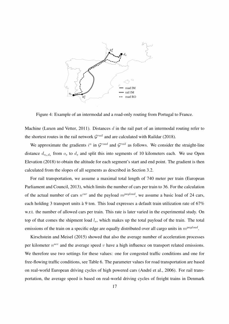
for such shipments. Figure 4 shows the RO and the IM routing for an exemplary shipment from
Portugal to France. In the figure, the solid lines present the pre- and post-haulage os → hos and
hds → ds in the road mode, the two parallel solid lines represent the rail transportation ho
s → hds
and the dashed line corresponds to the direct road transportation os → ds.
4.2. Specification of Emission Model Parameters
We now specify the trip specific parameters distance d, gradient i, payload mpayload, number
of rail cars ncar, average number of acceleration processes per kilometer nacc and average speed
v for a shipment s. We suppress here the shipment subscript s for reasons of readability. Further-
more, we specify the emission coefficient k for electric trains and derive an appropriate number of
shipments to simulate for each pair of countries.
Distances d in the road-only mode and in the pre- and post-haulage of intermodal routings refer
to the fastest routes in the road network Groad and are calculated with the Open Source Routing
16
Show ID
Origin
Destination
Hub Origin
Hub Destination
Nr.
1
2
3
4
5
6
7
8
9
10
11
12
13
14
15
16
17
18
19
20
21
22
23
24
25
26
27
28
29
30
31
32
33
34
35
36
37
38
39
40
41
42
road IM
rail IM
road RO𝑜𝑠
ℎ𝑠𝑑
𝑑𝑠
ℎ𝑠𝑜
Figure 4: Example of an intermodal and a road-only routing from Portugal to France.
Machine (Luxen and Vetter, 2011). Distances d in the rail part of an intermodal routing refer to
the shortest routes in the rail network Grail and are calculated with Raildar (2018).
We approximate the gradients iα in Groad and Grail as follows. We consider the straight-line
distance dos,ds from os to ds and split this into segments of 10 kilometers each. We use Open
Elevation (2018) to obtain the altitude for each segment’s start and end point. The gradient is then
calculated from the slopes of all segments as described in Section 3.2.
For rail transportation, we assume a maximal total length of 740 meter per train (European
Parliament and Council, 2013), which limits the number of cars per train to 36. For the calculation
of the actual number of cars ncar and the payload mpayload, we assume a basic load of 24 cars,
each holding 3 transport units à 9 ton. This load expresses a default train utilization rate of 67%
w.r.t. the number of allowed cars per train. This rate is later varied in the experimental study. On
top of that comes the shipment load ls, which makes up the total payload of the train. The total
emissions of the train on a specific edge are equally distributed over all cargo units in mpayload.
Kirschstein and Meisel (2015) showed that also the average number of acceleration processes
per kilometer nacc and the average speed v have a high influence on transport related emissions.
We therefore use two settings for these values: one for congested traffic conditions and one for
free-flowing traffic conditions, see Table 6. The parameter values for road transportation are based
on real-world European driving cycles of high powered cars (André et al., 2006). For rail trans-
portation, the average speed is based on real-world driving cycles of freight trains in Denmark
17

(Lindgreen and Sorenson, 2005b). The average number of acceleration processes is set to 1 per
100 km for free-flowing traffic conditions and to 1 per 10 km for congested traffic conditions. Note
that the average travel speed for rail transportation is rather high for congested traffic conditions.
This reflects the freight trains’ stop-and-go behavior, which is characterized by an acceleration to
full speed between the stops.
road rail
congested free-flowing congested free-flowing
average speed v [km/h] 40 80 70 80average accelerations nacc [per km] 2.5 0.12 0.1 0.01
Table 6: Traffic conditions for road and rail transportation.
For the well-to-wheel emission coefficient k for electric trains on edges Erail that belong to
country ci ∈ C, we use the energy mix of this particular country as reported in Moro and Lonza
(2017), see Table 1. Finally, if ferry transportation is part of the routing, we use an emission rate
of 51.35 gCO2e/ton-km for this leg, see DEFRA (2017).
Having discussed the generation and routing of shipments, as well as the emission model pa-
rameters, we can now identify the number of shipments that needs to be simulated for a country
pair (c1, c2) to obtain a valid estimate of the average emission rate. We derive this number from
an analysis of the convergence index (Jung et al., 2004). The convergence index compares the
deviation between the average rate observed after n ∈ [1, 2, . . . , N ] simulated shipments with
the average rate observed after simulating a total of N shipments. For this purpose, we simulate
N = 2000 heavy goods shipments for country pairs (POL, PRT) and (FRA, FRA). For the first
country pair, we expect similar routings for major parts of the journey and thus low variations in
the rates. For the second country pair, we expect a high share of pre- and post carriages of variable
length and thus higher variations in the rates. Figure 5 illustrates the observed convergence of
emission rates. The rates are higher for road only transportation than for intermodal transportation
but converge in both cases quickly to the final rate observed after N = 2000 simulated shipments.
For example, the intermodal emission rates for shipments within France are 20.06 gCO2e/ton-km
after simulating 500 shipments and 20.13 gCO2e/ton-km after simulating 2000 shipments. For
18

shipments between Poland and Portugal the rate is 16.64 gCO2e/ton-km after 500 shipments and
16.62 gCO2e/ton-km after 2000 shipments. From this analysis, we deduct that 500 shipments pro-
duce valid average emission rates and, therefore, we simulate |Sc1,c2| = 500 shipments for each
country pair (c1, c2).
Export Seite 2
0
10
20
30
40
50
60
70
0 250 500 750 1000 1250 1500 1750 2000
emis
sio
n r
ate
[gC
O2e/
ton
-km
]
number of shipments [-]
(POL, PRT) (FRA, FRA)
road-only
intermodal
Figure 5: Convergence of emission rates for country pairs (POL, PRT) and (FRA, FRA).
4.3. Definition of Simulation Configurations
We conduct our simulation study to calculate average emission rates for various relevant trans-
port situations. We consider varied parameters for shipments (cargo type, size), varied parameters
for the emission model (traffic conditions, gradient calculation) and miscellaneous settings of addi-
tional parameters (train utilization rates, empty return trips, a green power scenario and emissions
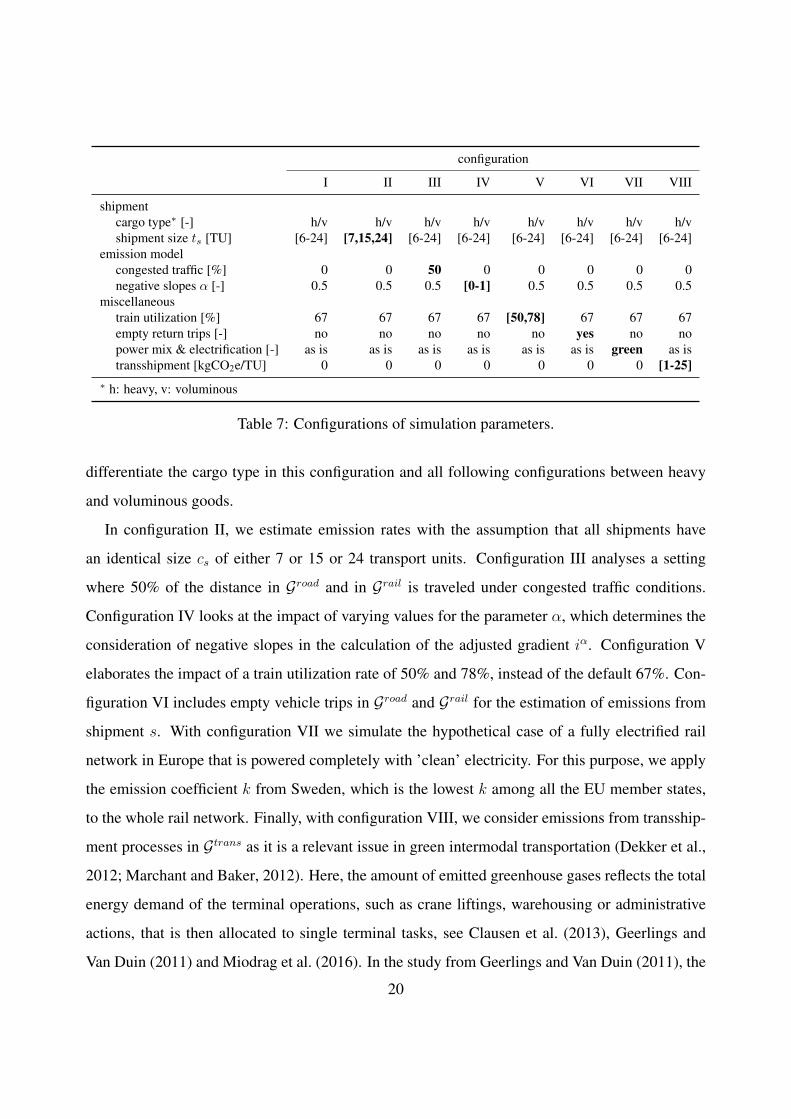
from transshipment operations). Table 7 provides an overview of all simulation settings. The de-
fault setting, configuration I, estimates emission rates with random shipment sizes between 6 and
24 transport units (TU), free-flowing traffic conditions, a value of α = 0.5 for computing the ad-
justed gradient, a train utilization rate of 67%, no empty return trips, the country specific electric
power mixes, the current degree of rail line electrification and no emissions from transshipment
operations. Since we expect that the cargo weight has a major impact on the emission rates, we19
configuration
I II III IV V VI VII VIII
shipmentcargo type∗ [-] h/v h/v h/v h/v h/v h/v h/v h/vshipment size ts [TU] [6-24] [7,15,24] [6-24] [6-24] [6-24] [6-24] [6-24] [6-24]
emission modelcongested traffic [%] 0 0 50 0 0 0 0 0negative slopes α [-] 0.5 0.5 0.5 [0-1] 0.5 0.5 0.5 0.5
miscellaneoustrain utilization [%] 67 67 67 67 [50,78] 67 67 67empty return trips [-] no no no no no yes no nopower mix & electrification [-] as is as is as is as is as is as is green as istransshipment [kgCO2e/TU] 0 0 0 0 0 0 0 [1-25]
∗ h: heavy, v: voluminous
Table 7: Configurations of simulation parameters.
differentiate the cargo type in this configuration and all following configurations between heavy
and voluminous goods.
In configuration II, we estimate emission rates with the assumption that all shipments have
an identical size cs of either 7 or 15 or 24 transport units. Configuration III analyses a setting
where 50% of the distance in Groad and in Grail is traveled under congested traffic conditions.
Configuration IV looks at the impact of varying values for the parameter α, which determines the
consideration of negative slopes in the calculation of the adjusted gradient iα. Configuration V
elaborates the impact of a train utilization rate of 50% and 78%, instead of the default 67%. Con-
figuration VI includes empty vehicle trips in Groad and Grail for the estimation of emissions from
shipment s. With configuration VII we simulate the hypothetical case of a fully electrified rail
network in Europe that is powered completely with ’clean’ electricity. For this purpose, we apply
the emission coefficient k from Sweden, which is the lowest k among all the EU member states,
to the whole rail network. Finally, with configuration VIII, we consider emissions from transship-
ment processes in Gtrans as it is a relevant issue in green intermodal transportation (Dekker et al.,
2012; Marchant and Baker, 2012). Here, the amount of emitted greenhouse gases reflects the total
energy demand of the terminal operations, such as crane liftings, warehousing or administrative
actions, that is then allocated to single terminal tasks, see Clausen et al. (2013), Geerlings and
Van Duin (2011) and Miodrag et al. (2016). In the study from Geerlings and Van Duin (2011), the
20

authors estimate values of 14 and 23 kgCO2 per container for two sea-rail transshipment terminals
in the Port of Rotterdam and elaborate that terminal layout is important for an accurate estimation.
An estimation of transshipment emissions for a 40-foot container in Clausen et al. (2013) yields 6
kgCO2e for a transshipment from sea to land and 12 kgCO2e for a transshipment between rail and
road. Since rail-road freight terminals can differ substantially in their layout, see Ballis and Golias
(2002), we simulate in configuration VIII values between 1 and 25 kgCO2e per transport unit and
per rail/road transshipment operation. With 27 countries considered in our study, 500 shipments
per country pair, and a differentiation between heavy and voluminous goods, we simulate a total
of 729,000 shipments for each of the eight configurations.
5. Results
Our results comprise estimated well-to-wheel emission rates in gCO2e/ton-km for 729 country
pairs. Emission rates reported for a country pair (c1, c2) are averages over the shipments s ∈ Sc1,c2 .
For the notation of the country pairs we use the country codes as reported in Table 1. We discuss in
the following the results of selected country pairs only and refer to the Appendix A for a complete
overview of all obtained results. A comprehensive summary of the results is shown in Table 8.
Details of the results for configuration I and II are described in Section 5.1. Section 5.2 provides
insights into the mesoscopic emission estimation model, including results from configurations III
and IV. Finally, Section 5.3 presents results from configurations V, VI, VII and VIII.
emission rates for heavy goods [gCO2e/ton-km] emission rates for voluminous goods [gCO2e/ton-km]
config. road (RO) intermodal (IM) rail section IM-share∗ road (RO) intermodal (IM) rail section IM-share∗
I 56.8 23.8 18.1 92.7 86.7 29.2 19.4 94.9II [55.5-60.7] [23.1-24.9] [17.6-18.7] [92.7-93.1] [84.3-93.6] [28.9-30.2] [19.3-19.4] [94.8-95.3]III 64.8 25.7 19.0 93.5 95.6 31.2 20.2 95.2IV [48.8-64.9] [17.7-30.0] [12.5-23.8] [89.6-94.6] [75.9-97.4] [22.5-36.0] [13.5-25.3] [93.8-95.7]V 56.8 [23.6-24.3] [17.9-18.7] [92.3-92.8] 86.7 [28.8-30.1] [19.0-20.4] [94.7-95.0]VI 92.6 32.3 21.9 94.7 152.2 44.7 26.4 95.7VII 56.8 10.1 2.2 96.9 86.7 14.5 2.3 97.0VIII 56.8 [23.8-26.6] 18.1 [89.1-92.7] 86.7 [29.2-34.4] 19.4 [91.7-94.9]∗ intermodal share (IM-share) in %, see Section 5.1
Table 8: Aggregated results for simulation configurations I to VIII.
21

5.1. General Findings
In this section, we look at the spread of emission rates for the 729 country pairs under configu-
ration I. We analyze emission rates from heavy and voluminous goods and we compare rates from
road-only routing with rates from intermodal routing. Furthermore, we analyze the impact of the
shipment size using configuration II.
A comparison of the emission rates across all country pairs shows that there is a wide spread
of emission rates. Figure 6 shows the relative frequency of emission rates from heavy shipments
(Figure 6a) and voluminous shipments (Figure 6b) over all 729 country pairs. In general, inter-
modal routing (black bars) leads to lower average rates than road-only routing (grey bars), which
confirms the advantage of rail transportation with respect to eco-friendliness. This finding is in
line with other studies like those in Table 2. From our extensive simulation, we observe that emis-
sion rates from IM routings are on average 58% below rates from RO routings for heavy goods.
For voluminous goods this measure is 66%. Emission rates for IM routings of both heavy and vo-
luminous goods are mostly within a range of 15 to 45 gCO2e/ton-km. For RO routings, emissions
for heavy goods are mostly between 50 to 70 gCO2e/ton-km and for voluminous goods between
80 to 100 gCO2e/ton-km. The distribution of RO emissions is positively skewed at rates of about
50 for heavy shipments and about 80 gCO2e/ton-km for voluminous shipments, see Figure 6. This
is because the gradient of a route is a major driver of RO emissions, where all country pairs with
negligible altitude differences get close to these lower bounds. In contrast, for IM shipments,
many more relevant drivers exist (traction type, power mix, etc.) which affects a more symmetric
distribution of emission rates.
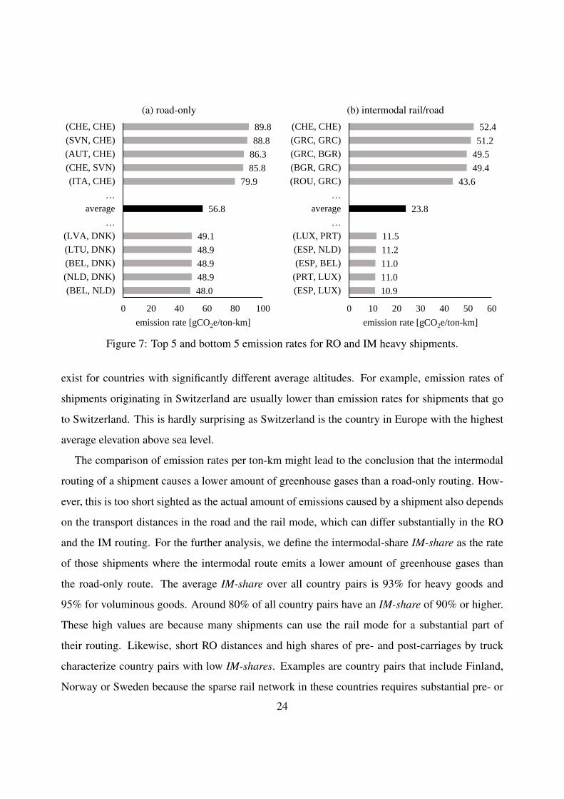
Figure 7 shows the average and extreme emission rates from RO and IM routings of heavy
goods under configuration I. The analysis shows that the extreme values for RO routing result
from geographical characteristics, such as mountains. Routes with high emission rates pass the
Alps, the highest mountain range in Europe, and routes with low emission rates typically involve
flat terrain, as is found in Denmark, the Netherlands, Belgium, etc.. In contrast, extreme values
from IM routing result from the characteristics of a country’s rail system, such as the share of
electrification or the used power mix. High emissions are found for Greece, where just about
half of the rail lines are electrified in combination with an unfavorable emission coefficient (see22

(a) heavy shipments
0
2
4
6
8
10
12
0 15 30 45 60 75 90 105 120 135
rela
tiv
e fr
equ
ency
[%
]
emission rate [gCO2e/ton-km]
intermodal
road-only
(b) voluminous shipments
0
2
4
6
8
10
12
0 15 30 45 60 75 90 105 120 135
rela
tiv
e fr
equ
ency
[%
]
emission rate [gCO2e/ton-km]
intermodal
road-only
Figure 6: Relative frequency of emission rates.
Table 1) that results from using lignite (brown coal) as a major source of energy (Public Power
Corporation S.A., 2016). Low emissions are found for routes where substantial parts of the rail
transportation goes through France, such as (PRT, LUX) or (ESP, BEL), as most of the rail network
is electrified in combination with a low CO2e-emission coefficient (see Table 1) that results from
using nuclear power as a major source of energy (Réseau de Transport d’Électricité, 2017). The
spread of emission rates for heavy RO transportation is between 48.0 and 89.8 gCO2e/ton-km with
an average of 56.8 gCO2e/ton-km. For heavy IM transportation, the spread is between 10.9 and
52.4 gCO2e/ton-km with an average of 23.8 gCO2e/ton-km. These observations indicate that the
use of a single average emission rate for a large area like Europe can lead to large errors in the
estimation of emissions for a particular transport relation or a particular shipment.
The emission rates from shipments with voluminous goods are higher than the emission rates
from shipments with heavy goods, see Table 8. For example, the average rate over all country pairs
from RO routing is 56.8 gCO2e/ton-km for heavy goods and 86.7 gCO2e/ton-km for voluminous
goods. For IM routing, the rate is 23.8 gCO2e/ton-km for heavy goods and 29.2 gCO2e/ton-km for
voluminous goods. This finding shows that emission rates from road-only and intermodal routing
are both sensitive to additional weight. This motivates presenting separate emission rates for heavy
goods and for voluminous goods in all considered simulation configurations. We furthermore
observe that the direction of a route can have an impact, i.e. that the results for country pair
(c1, c2) and country pair (c2, c1) are not necessarily identical. However, such differences primarily
23
(a) road-only
48.0
48.9
48.9
48.9
49.1
56.8
79.9
85.8
86.3
88.8
89.8
0 20 40 60 80 100
(BEL, NLD)
(NLD, DNK)
(BEL, DNK)
(LTU, DNK)
(LVA, DNK)
…
average
…
(ITA, CHE)
(CHE, SVN)
(AUT, CHE)
(SVN, CHE)
(CHE, CHE)
emission rate [gCO2e/ton-km]
(b) intermodal rail/road
10.9
11.0
11.0
11.2
11.5
23.8
43.6
49.4
49.5
51.2
52.4
0 10 20 30 40 50 60
(ESP, LUX)
(PRT, LUX)
(ESP, BEL)
(ESP, NLD)
(LUX, PRT)
…
average
…
(ROU, GRC)
(BGR, GRC)
(GRC, BGR)
(GRC, GRC)
(CHE, CHE)
emission rate [gCO2e/ton-km]
Figure 7: Top 5 and bottom 5 emission rates for RO and IM heavy shipments.
exist for countries with significantly different average altitudes. For example, emission rates of
shipments originating in Switzerland are usually lower than emission rates for shipments that go
to Switzerland. This is hardly surprising as Switzerland is the country in Europe with the highest
average elevation above sea level.
The comparison of emission rates per ton-km might lead to the conclusion that the intermodal
routing of a shipment causes a lower amount of greenhouse gases than a road-only routing. How-
ever, this is too short sighted as the actual amount of emissions caused by a shipment also depends
on the transport distances in the road and the rail mode, which can differ substantially in the RO
and the IM routing. For the further analysis, we define the intermodal-share IM-share as the rate
of those shipments where the intermodal route emits a lower amount of greenhouse gases than
the road-only route. The average IM-share over all country pairs is 93% for heavy goods and
95% for voluminous goods. Around 80% of all country pairs have an IM-share of 90% or higher.
These high values are because many shipments can use the rail mode for a substantial part of
their routing. Likewise, short RO distances and high shares of pre- and post-carriages by truck
characterize country pairs with low IM-shares. Examples are country pairs that include Finland,
Norway or Sweden because the sparse rail network in these countries requires substantial pre- or
24

post-carriages by truck. The IM-share is also low for country pairs with low electrification of
the rail network or with high emission coefficients. For example, the IM-share for (GRC, BGR)
is 48% for shipments with heavy goods and 79% for shipments with voluminous goods. This is
because only half of the rail lines in Greece are electrified and both countries Greece and Bulgaria
have a power mix with high emission coefficients, see Table 1.
The size ts of a shipment s influences the number of trucks required, respectively the number of
rail cars in the IM routing. Figure 8 shows the average rates across all country pairs for shipments
with random sizes (configuration I) and fixed sizes of 7 or 15 or 24 transport units (configuration
II). The results show that the shipment size has only a small impact on the observed emission
rates in RO routings. Since we consider quite large shipments of multiple transport units in all
experiments, road-only emissions do not differ between even numbers of transport units and the
only variance results from shipments with an uneven number of transport units. In this case,
the relative impact of the emissions of the single half-filled truck depreciates with larger shipment
size and the average emission rates tend towards the emission rates with even numbers of transport
units. The impact of the shipment size is even lower in IM routings. The marginal emissions of an
additional transport unit are very low, which is because of the high tare weight of trains and their
substantial base utilization of 67%.
93.6
60.7
30.224.9
88.6
57.9
29.423.9
84.3
55.5
28.923.1
86.7
56.8
29.223.8
0
20
40
60
80
100
emis
sio
n r
ate
[gC
O2e/
ton-k
m]
7 15 24 rand. 7 15 24 rand. 7 15 24 rand. 7 15 24 rand.
voluminous heavy voluminous heavy
road-only intermodal
Figure 8: Emission rates from fixed shipment sizes (grey bars) and random sizes (black bars).
25
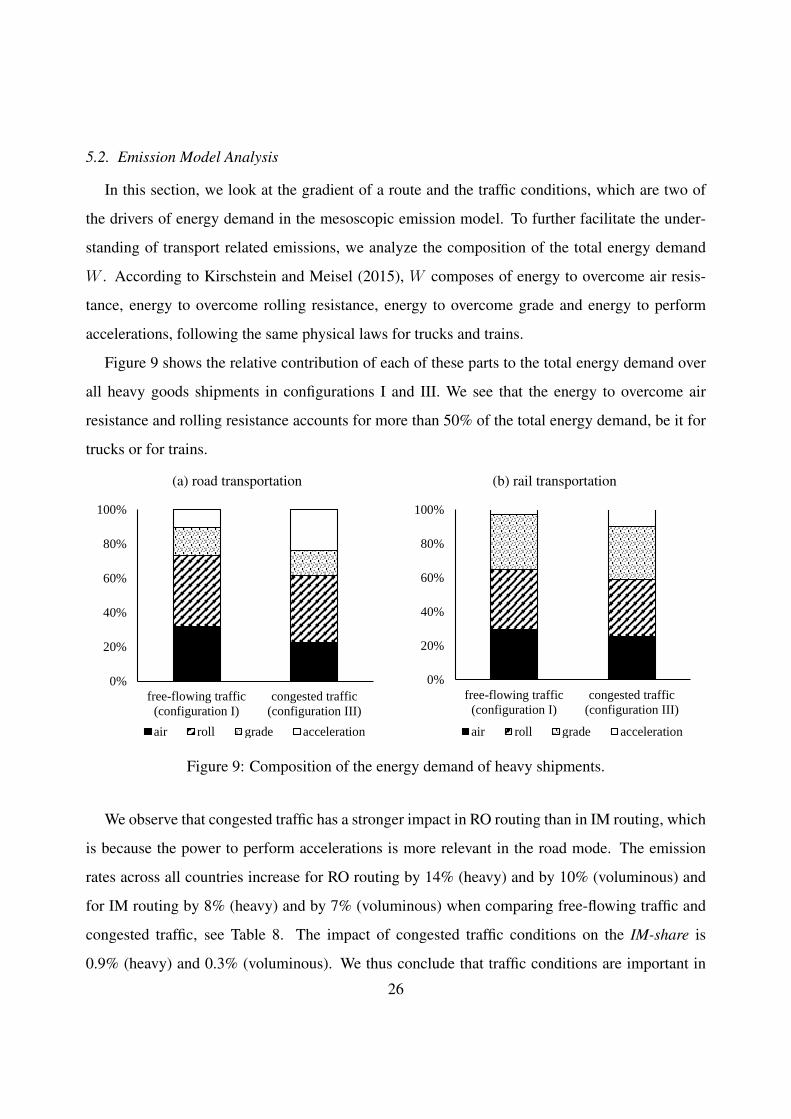
5.2. Emission Model Analysis
In this section, we look at the gradient of a route and the traffic conditions, which are two of
the drivers of energy demand in the mesoscopic emission model. To further facilitate the under-
standing of transport related emissions, we analyze the composition of the total energy demand
W . According to Kirschstein and Meisel (2015), W composes of energy to overcome air resis-
tance, energy to overcome rolling resistance, energy to overcome grade and energy to perform
accelerations, following the same physical laws for trucks and trains.
Figure 9 shows the relative contribution of each of these parts to the total energy demand over
all heavy goods shipments in configurations I and III. We see that the energy to overcome air
resistance and rolling resistance accounts for more than 50% of the total energy demand, be it for
trucks or for trains.
(a) road transportation
0%
20%
40%
60%
80%
100%
free-flowing traffic
(configuration I)
congested traffic
(configuration III)
air roll grade acceleration
(b) rail transportation
0%
20%
40%
60%
80%
100%
free-flowing traffic
(configuration I)
congested traffic
(configuration III)
air roll grade acceleration
Figure 9: Composition of the energy demand of heavy shipments.
We observe that congested traffic has a stronger impact in RO routing than in IM routing, which
is because the power to perform accelerations is more relevant in the road mode. The emission
rates across all countries increase for RO routing by 14% (heavy) and by 10% (voluminous) and
for IM routing by 8% (heavy) and by 7% (voluminous) when comparing free-flowing traffic and
congested traffic, see Table 8. The impact of congested traffic conditions on the IM-share is
0.9% (heavy) and 0.3% (voluminous). We thus conclude that traffic conditions are important in
26

estimating the height of emissions for a specific transport relation but they hardly determine which
routing (RO or IM) is more eco-friendly.
With configuration IV, we look at the influence of considering energy from negative slopes
through the average adjusted gradient iα. For α = 0, the adjusted gradient considers no energy
from negative slopes at all. For α = 1, where all energy from negative slopes is recovered, iα
reflects the simple origin-destination altitude difference and is identical to gradient i. For these
extreme values, the average emission rate for heavy shipments over all country pairs is 17.7 (α =
1) and 30.0 (α = 0) for IM routings whereas it is 48.8 (α = 1) and 64.9 (α = 0) for RO routings.
This supports the observation from Figure 9 where the relative energy demand to overcome grade
is higher for rail transportation than for road transportation. Clearly, these results vary among
country pairs. Figure 10 shows individual rates for six exemplary country pairs where shipments
originate in the Netherlands with values of α being set to 0, 0.2, . . . 1. All country pairs have a
similar emission rate for the case α = 1, although their geographical characteristics are quite
different. Shipments to Denmark, Estonia and Poland do not pass significant elevations, while
shipments to Portugal, Bulgaria and Italy have to go through mountain ranges. Emission rates that
are calculated with α = 1 do not reflect these differences, whereas for lower values of α we see a
clear spread in the emission rates that reflects these geographical characteristics. We thus conclude
that the adjusted gradient iα can better capture the characteristics of the diverse transport relations.
40
50
60
70
80
0 0.2 0.4 0.5 0.6 0.8 1
emis
sio
n r
ate
[gC
O2e/
ton-k
m]
downhill slope weight α [-]
(NLD, ITA)
(NLD, BGR)
(NLD, PRT)
(NLD, POL)
(NLD, EST)
(NLD, DNK)
Figure 10: Exemplary emission rates of heavy goods from configuration IV.
27
5.3. Further Configurations
This section looks at the impact of varying train utilization (configuration V), empty returns
trips (configuration VI), a fully electrified railway network (configuration VII) and emissions from
transshipment operations (configuration VIII). For these configurations, we focus on discussing
the aggregated results from Table 8. While configuration I assumes a train utilization rate of
67%, configuration V addresses utilization rates of 50% and 78%. We observe that a higher train
utilization rate, expressed through a larger number of transport units and rail cars for the basic
load, causes less marginal greenhouse gases from shipment load ls and thus reduces the emission
rate of shipment s. Likewise, a lower train utilization rate allocates more greenhouse gases to s.
However, the absolute change is very low such that the average rate for heavy goods in IM routings
varies between 23.6 for a train utilization of 78% and 24.3 gCO2e/ton-km for a utilization of 50%.
For voluminous goods the rate varies between 28.8 and 30.1 gCO2e/ton-km. Since there is hardly
any impact on the IM emission rate, there is also hardly any change on the IM-share.
The European Norm DIN EN 16258 (2012) states that emissions from transportation should
also include vehicle operations from empty trips. Our results so far completely ignored empty
trips. With configuration VI, we now consider this and assume empty vehicle return trips for all
shipments. For this, we consider for a shipment s a corresponding shipment s′ with os′ = ds and
ds′ = os and load ls′ = 0. The IM routing for the return trip s′ of shipment s is then ds to hds via
road, hds to ho
s via rail and hos to os via road. As expected, the consideration of empty return trips
leads to a strong increase in the average emission rates of the freight shipments. The rate across
all country pairs increases for RO routing by 63% (heavy) and by 75% (voluminous) and for IM
routing by 36% (heavy) and by 53% (voluminous), respectively. Despite of this, we only observe
a small increase in the IM-share by 2.0% (heavy) and 0.8% (voluminous), see Table 8.
With configuration VII, we analyze the scenario of a fully electrified railway network. Further-
more, we apply a low emission coefficient of k = 45 gCO2e/kWh to the whole network. This
coefficient stems from Sweden, which is the EU member state with the lowest k. As expected,
the emission rates from freight transportation on rail sections decrease for nearly all country pairs
with an average reduction of around 88%, see Table 8. This also leads to increasing IM-shares.
Since the majority of country pairs already have high IM-shares in the base setting (configuration28

I) we see an increase of this measure of merely 4.2% for heavy goods and 2.1% for voluminous
goods in configuration VII. Still, for some country pairs, we observe a much stronger impact of
the green and fully electrified rail system. This is the case for countries that currently have high
electric emission coefficients, like Latvia, Poland or Estonia. With a total of 438 billion ton-km of
rail freight transport in the EU in 2016 (Eurostat, 2018c) and an average reduction of rail emission
by 88% in a completely green rail network, the total amount of anthropogenic CO2e emissions
could be reduced by approximately 7.25 million tons.
Finally, in configuration VIII, we consider emissions released during transshipment processes
in the intermodal routing. Each of these routings includes two transshipment operations (one from
road to rail and one from rail to road) where we assume an identical emission rate per transship-
ment operation. We varied this rate in the range 1 to 25 kgCO2e per transshipped transport unit.
Figure 11 shows the average IM-share across all countries depending on the emission rate per
transshipment operation. Surprisingly, we only observe a very small and constant decrease of
about 0.1% per kgCO2e added to the transshipment emission rate. However, we observe that the
impact on the intermodal emission rates can be high for some country pairs. Here, the distance be-
tween shipments is the most important driver. This is because the emissions from transshipmentsExport: page 3
80
85
90
95
100
0 5 10 15 20 25
IM-s
har
e [%
]
emission rate per transshipment operation [kgCO2e/TU]
heavy voluminous
linear regression (voluminous):
y = -0.1289x + 94.996
R² = 0.9993
linear regression (heavy):
y = -0.1429x + 92.72
R² = 0.9995
Figure 11: IM-share depending on the emission rate per transshipment operation.
29
(a) difference per country pair (heavy goods)
0.82
0.82
0.84
0.84
0.90
2.87
12.86
12.99
13.71
18.14
19.72
0 5 10 15 20 25
(PRT, GRC)
(GRC, PRT)
(FIN, PRT)
(PRT, FIN)
(EST, PRT)
...
average
...
(NLD, BEL)
(BEL, LUX)
(SVN, SVN)
(NLD, NLD)
(BEL, BEL)
Δ emission rate [gCO2e/ton-km]
(b) difference dependent on the average distance
0
5
10
15
20
0 1000 2000 3000 4000
Δem
issi
on r
ate
[gC
O2e/
ton-k
m]
average distance [km]
heavy
voluminous
Figure 12: Change of IM emissions rates for transshipment emissions of 25 kgCO2e/TU.
are a fixed amount per shipment, which leads to a depreciation of these emissions with increasing
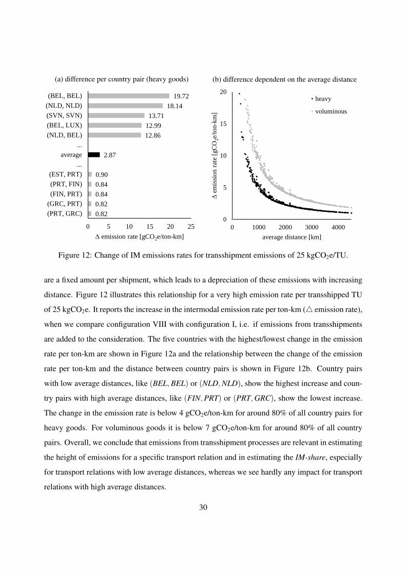
distance. Figure 12 illustrates this relationship for a very high emission rate per transshipped TU
of 25 kgCO2e. It reports the increase in the intermodal emission rate per ton-km (4 emission rate),
when we compare configuration VIII with configuration I, i.e. if emissions from transshipments
are added to the consideration. The five countries with the highest/lowest change in the emission
rate per ton-km are shown in Figure 12a and the relationship between the change of the emission
rate per ton-km and the distance between country pairs is shown in Figure 12b. Country pairs
with low average distances, like (BEL, BEL) or (NLD, NLD), show the highest increase and coun-
try pairs with high average distances, like (FIN, PRT) or (PRT, GRC), show the lowest increase.
The change in the emission rate is below 4 gCO2e/ton-km for around 80% of all country pairs for
heavy goods. For voluminous goods it is below 7 gCO2e/ton-km for around 80% of all country
pairs. Overall, we conclude that emissions from transshipment processes are relevant in estimating
the height of emissions for a specific transport relation and in estimating the IM-share, especially
for transport relations with low average distances, whereas we see hardly any impact for transport
relations with high average distances.
30
6. Conclusion
In this paper, we have calculated emission rates of intermodal rail/road and road-only trans-
portation of large cargo shipments in Europe. We have described the intermodal rail/road network,
the various data sources and the results from a comprehensive simulation study. We found that
the average emission rate across all country pairs from road-only routing is 57 gCO2e/ton-km for
heavy goods and 87 gCO2e/ton-km for voluminous goods. For intermodal routing, we determined
rates of 24 gCO2e/ton-km for heavy goods and 29 gCO2e/ton-km for voluminous goods. How-
ever, there are high variations. Rates for road transportation range from 48 to 131 gCO2e/ton-km
over the considered 729 country pairs. Rates for intermodal transportation range from 11 to 72
gCO2e/ton-km. The highest emission rates are observed for transports that go through the Alps.
Furthermore, we found that intermodal routings emit less greenhouse gases than road-only rout-
ings for over 90% of the simulated shipments. Again, this value varies among country pairs and
is significantly lower for countries with many non-electrified rail tracks and high emission coeffi-
cients for their electricity. In our study, we have identified emission factors that quantify the value
of road-only and intermodal emission rates and thus determine which routing is more eco-friendly.
Some of these factors are of geographical or physical nature, such as gradient of the route or ve-
hicle size, and thus rather hard or even impossible to change by decision makers from industry.
Other factors, like average speed or the share of electrified rail lines, are set by transport operators
or public authorities and thus could be addressed by policies that target a reduction of greenhouse
gases from freight transportation.
Overall, our results indicate that the use of a single average emission rate for a large area like
Europe can lead to substantial errors in the estimation of emissions for individual shipments or
particular transport relations. The appendix of this study therefore provides look-up tables for
all country pairs and shows the respective emission rates from road, rail and intermodal rail/road
transportation as well as the IM-share for all considered scenarios. Future research should put a
scope on smaller shipments and the impact of freight consolidation. It is also of interest to identify
realistic values for the gradient parameter α and to validate our emission estimates through real-
work experiment. Finally, we see the in-depth consideration of emissions from transshipment
31

processes as another field of research for gaining deeper insights into the drivers of eco-friendly
freight transportation.
Acknowledgments
This research was supported by the German Research Foundation (DFG) under reference ME3586/1-1. We thank two anonymous reviewers for their valuable comments which helped to im-prove the manuscript considerably.
Appendix A. Supplementary data
Supplementary data associated with this article can be found in the online version of this article andon the website of our department (https://www.scm.bwl.uni-kiel.de/de/forschung/research-data).
Bibliography
André, M., Joumard, R., Vidon, R., Tassel, P., Perret, P., 2006. Real-world european driving cycles, for measuringpollutant emissions from high-and low-powered cars. Atmospheric Environment 40 (31), 5944–5953.
Ballis, A., Golias, J., 2002. Comparative evaluation of existing and innovative rail–road freight transport terminals.Transportation Research Part A: Policy and Practice 36 (7), 593–611.
Bauer, J., Bektas, T., Crainic, T. G., 2010. Minimizing greenhouse gas emissions in intermodal freight transport: anapplication to rail service design. Journal of the Operational Research Society 61 (3), 530–542.
Behnke, M., Kirschstein, T., 2017. The impact of path selection on GHG emissions in city logistics. TransportationResearch Part E: Logistics and Transportation Review 106, 320–336.
Bektas, T., Laporte, G., 2011. The pollution-routing problem. Transportation Research Part B: Methodological 45 (8),1232–1250.
BluFerries, 2018. BluFerries: Gruppo Ferrovie Dello Stato Italiane. http://www.bluferries.it/laflotta.html (visited on25.07.2018).
Clausen, U., Kaffka, J., Döring, L., Ebel, G., 2013. Container based calculation of greenhouse gas emissions - Amethod to determine emissions of container handlings in container terminals. General Proceedings of the 13thWorld Conference on Transport Research (WCTR).
Comer, B., Corbett, J. J., Hawker, J. S., Korfmacher, K., Lee, E. E., Prokop, C., Winebrake, J. J., 2010. Marine vesselsas substitutes for heavy-duty trucks in great lakes freight transportation. Journal of the Air & Waste ManagementAssociation 60 (7), 884–890.
Craig, A. J., Blanco, E. E., Sheffi, Y., 2013. Estimating the CO2 intensity of intermodal freight transportation. Trans-portation Research Part D: Transport and Environment 22, 49–53.
de Miranda Pinto, J. T., Mistage, O., Bilotta, P., Helmers, E., 2017. Road-rail intermodal freight transport as a strategyfor climate change mitigation. Environmental Development 25, 100–110.
DEFRA, 2017. Department for Environment, Food and Rural Affairs. Greenhouse Gas Reporting: Conversion Factors2017. https://www.gov.uk/government/publications/greenhouse-gas-reporting-conversion-factors-2017 (visited on25.07.2018).
Dekker, R., Bloemhof, J., Mallidis, I., 2012. Operations Research for green logistics - An overview of aspects, issues,contributions and challenges. European Journal of Operational Research 219 (3), 671–679.
DeLuchi, M. A., 1991. Emissions of greenhouse gases from the use of transportation fuels and electricity. Tech. rep.,Argonne National Lab.
32

Demir, E., Bektas, T., Laporte, G., 2011. A comparative analysis of several vehicle emission models for road freighttransportation. Transportation Research Part D: Transport and Environment 16 (5), 347–357.
DIN EN 16258, 2012. Methodology for calculation and declaration of energy consumption and GHG emissions oftransport services (freight and passengers). European Committee for Standardization.
EcoTransIT World Initiative, 2016. EcoTransIT: Ecological Transport Information Tool for Worldwide Transports,Methodology and Data (30.06.2016). http://www.ecotransit.org/download/ETW_Methodology_Background_Report_2016.pdf (visited on 25.07.2018).
Ehmke, J. F., Campbell, A. M., Thomas, B. W., 2016. Data-driven approaches for emissions-minimized paths in urbanareas. Computers & Operations Research 67, 34–47.
European Commission, 2015. State aid: Commission approves public financing of Fehmarn Belt fixed rail-road link.http://europa.eu/rapid/press-release_IP-15-5433_en.htm (visited on 25.07.2018).
European Commission, 2018. About TEN-T. http://ec.europa.eu/transport/infrastructure/tentec/tentec-portal/site/en/abouttent.htm (visited on 25.07.2018).
European Parliament, 2017. Parliamentary Questions: Tallinn-Helsinki tunnel. http://www.europarl.europa.eu/sides/getDoc.do?type=WQ&reference=E-2017-004271&language=EN (visited on 25.07.2018).
European Parliament and Council, 2013. Regulation (EU) No 1315/2013 of the European Parliament and the Coun-cil of 11 December 2013 on Union guidelines for the development of the trans-European transport network andrepealing Decision No 661/2010/EU. http://data.europa.eu/eli/reg/2013/1315/oj (visited on 25.07.2018).
Eurostat, 2018a. Freight transport statistics - modal split. http://ec.europa.eu/eurostat/statistics-explained/index.php/Freight_transport_statistics_-_modal_split (visited on 25.07.2018).
Eurostat, 2018b. Greenhouse gas emissions by source sector. http://ec.europa.eu/eurostat/statistics-explained/index.php?title=Greenhouse_gas_emission_statistics (visited on 25.07.2018).
Eurostat, 2018c. Railway freight transport statistics. http://ec.europa.eu/eurostat/statistics-explained/index.php?title=Railway_freight_transport_statistics (visited on 25.07.2018).
Geerlings, H., Van Duin, R., 2011. A new method for assessing CO2-emissions from container terminals: a promisingapproach applied in Rotterdam. Journal of Cleaner Production 19 (6-7), 657–666.
Geofabrik, 2018. OpenStreetMap Data Extracts. http://download.geofabrik.de/ (visited on 25.07.2018).Hawker, J. S., Comer, B., Corbett, J. J., Ghosh, A., Korfmacher, K., Lee, E. E., Li, B., Prokop, C., Winebrake,
J. J., 2010. An integrated model to study environmental, economic, and energy trade-offs in intermodal freighttransportation. 5th International Congress on Environmental Modelling and Software. Ottawa. Canada.
Hickman, J., Hassel, D., Joumard, R., Samaras, Z., Sorenson, S., 1999. Methodology for calculating transport emis-sions and energy consumption. https://trimis.ec.europa.eu/sites/default/files/project/documents/meet.pdf (visitedon 25.07.2018).
Hoffrichter, A., Miller, A. R., Hillmansen, S., Roberts, C., 2012. Well-to-wheel analysis for electric, diesel andhydrogen traction for railways. Transportation Research Part D: Transport and Environment 17 (1), 28–34.
Jung, J. Y., Blau, G., Pekny, J. F., Reklaitis, G. V., Eversdyk, D., 2004. A simulation based optimization approach tosupply chain management under demand uncertainty. Computers & chemical engineering 28 (10), 2087–2106.
Kirschstein, T., Meisel, F., 2015. GHG-emission models for assessing the eco-friendliness of road and rail freighttransports. Transportation Research Part B: Methodological 73, 13–33.
Lindgreen, E. B. G., Sorenson, S. C., 2005a. Driving resistance from railroad trains. Tech. rep., Technical Universityof Denmark. Department of Mechanical Engineering.
Lindgreen, E. B. G., Sorenson, S. C., 2005b. Simulation of energy consumption and emissions from rail traffic. Tech.rep., Technical University of Denmark. Department of Mechanical Engineering.
Luxen, D., Vetter, C., 2011. Real-time routing with OpenStreetMap data. In: Proceedings of the 19th ACM SIGSPA-TIAL International Conference on Advances in Geographic Information Systems. GIS ’11. ACM, New York, NY,USA, pp. 513–516.
Marchant, C., Baker, P., 2012. Reducing the environmental impact of warehousing. In: McKinnon, A., Browne, M.,Whiteing, A. (Eds.), Green logistics: Improving the environmental sustainability of logistics, 2nd Edition. KoganPage Limited London, Ch. 8, pp. 175–202.
McKinnon, A., Browne, M., Whiteing, A., 2012. Green logistics: Improving the environmental sustainability oflogistics, 2nd Edition. Kogan Page Publishers.
33

Miodrag, Z., Kaffka, J., Clausen, U., Munsel, L., Drost, S., 2016. Assessment of emissions caused by logisticshandling operations in multimodal-terminals. Transportation Research Procedia 14, 2754–2761.
MMEEC, 2018. Multi-Modal Energy and Emissions Calculator (MMEEC). Rochester Institute of Technology andUniversity of Delaware. http://clarke.main.ad.rit.edu/LECDM/EmissionsCalc/ (visited on 25.07.2018).
Moro, A., Lonza, L., 2017. Electricity carbon intensity in European Member States: Impacts on GHG emissionsof electric vehicles. Transportation Research Part D: Transport and Environment. in press (corrected proof). doi:https://doi.org/10.1016/j.trd.2017.07.012.
NTM, 2017a. Network For Transport Measures: Rail cargo transport baselines 2017. https://www.transportmeasures.org/en/wiki/evaluation-transport-suppliers/rail-cargo-transport-baselines-2017/ (visited on 25.07.2018).
NTM, 2017b. Network For Transport Measures: Road cargo transport baselines 2017. https://www.transportmeasures.org/en/wiki/evaluation-transport-suppliers/road-transport-baselines-2017/ (visited on 25.07.2018).
Open Elevation, 2018. Open Elevation: A free and open-source elevation API. https://www.open-elevation.com (vis-ited on 25.07.2018).
Open Street Map, 2018. OpenStreetMap is the free wiki world map. https://www.openstreetmap.org (visited on25.07.2018).
Psaraftis, H. N., Kontovas, C. A., 2016. Transportation Emissions: Some Basics. In: Green Transportation Logistics.Springer, pp. 41–79.
Public Power Corporation S.A., 2016. Annual Report: January 1st, 2016 - December 31st, 2016. https://www.dei.gr/Documents2/ANNUAL%20REPORT/AR-2016/Annual_Report_2016_EN_WEB.pdf (visited on 25.07.2018).
Raildar, 2018. raildar.fr. http://raildar.fr/osrm/osrm.html (visited on 25.07.2018).Ross, M., 1997. Fuel efficiency and the physics of automobiles. Contemporary Physics 38 (6), 381–394.Réseau de Transport d’Électricité, 2017. RTE Open Data platform: Annual French electricity production (TWh) by
branch (2017). https://opendata.rte-france.com/explore/dataset/prod_par_filiere/table/?sort=-annee&refine.annee=2017 (visited on 25.07.2018).
Rudi, A., Fröhling, M., Zimmer, K., Schultmann, F., 2016. Freight transportation planning considering carbon emis-sions and in-transit holding costs: a capacitated multi-commodity network flow model. EURO Journal on Trans-portation and Logistics 5 (2), 123–160.
Scora, G., Barth, M., 2006. Comprehensive modal emissions model (CMEM), version 3.01 (Users guide). Centre forEnvironmental Research and Technology. University of California, Riverside.
Southworth, F., Peterson, B. E., 2000. Intermodal and international freight network modeling. Transportation ResearchPart C: Emerging Technologies 8 (1), 147–166.
Stead, D., 1999. Relationships between transport emissions and travel patterns in Britain. Transport Policy 6 (4), 247– 258.
StenaLine, 2018. StenaLineFreight / Routes and Ports / Trelleborg-Rostock. https://www.stenalinefreight.com/Routes-and-ports/trelleborg-rostock (visited on 25.07.2018).
TEN-T Compliance Maps, 2014. TEN-T Compliance Maps. TENtec Reporting. European Commission. https://ec.europa.eu/transport/themes/infrastructure/downloads_en (visited on 25.07.2018).
TENtec Interactive Map, 2018. TENtec Interactive Map Viewer. http://ec.europa.eu/transport/infrastructure/tentec/tentec-portal/map/maps.html (visited on 25.07.2018).
Wang, M. Q., 1999. Greet 1.5-transportation fuel-cycle model-vol. 1: methodology, development, use, and results.Tech. rep., Argonne National Lab., IL (US).
WebGIFT, 2018. Online Application of the Geospatial Intermodal Freight Transportation (GIFT) model. RochesterInstitute of Technology and University of Delaware. http://clarke.main.ad.rit.edu/LECDM/Webgift/ (visited on25.07.2018).
Winebrake, J. J., Corbett, J. J., Falzarano, A., Hawker, J. S., Korfmacher, K., Ketha, S., Zilora, S., 2008. Assessingenergy, environmental, and economic tradeoffs in intermodal freight transportation. Journal of the Air & WasteManagement Association 58 (8), 1004–1013.
34


