

Energy-efficient Optimization ofRailway Operation
An Algorithm Based on Kronecker Algebra
DISSERTATION
zur Erlangung des akademischen Grades
Doktor der technischen Wissenschaften
eingereicht von
Dipl.-Ing. Mark Volcic, BScMatrikelnummer 0425294
an derFakultät für Informatik der Technischen Universität Wien
Betreuung:Ao. Univ. Prof. Dipl.-Ing. Dr.techn. Johann BliebergerPriv. Doz. Dipl.-Ing. Dr.techn. Andreas Schöbel
Diese Dissertation haben begutachtet:
(Ao. Univ. Prof. Dipl.-Ing.Dr.techn. Johann Blieberger)
(Prof. Dr.-Ing. habil. JürgenSiegmann)
Wien, 29.12.2014(Dipl.-Ing. Mark Volcic, BSc)
Technische Universität WienA-1040 Wien � Karlsplatz 13 � Tel. +43-1-58801-0 � www.tuwien.ac.at


Energy-efficient Optimization ofRailway Operation
An Algorithm Based on Kronecker Algebra
DISSERTATION
submitted in partial fulfillment of the requirements for the degree of
Doktor der technischen Wissenschaften
by
Dipl.-Ing. Mark Volcic, BScRegistration Number 0425294
to the Faculty of Informaticsat the Vienna University of Technology
Advisor:Ao. Univ. Prof. Dipl.-Ing. Dr.techn. Johann BliebergerPriv. Doz. Dipl.-Ing. Dr.techn. Andreas Schöbel
The dissertation has been reviewed by:
(Ao. Univ. Prof. Dipl.-Ing.Dr.techn. Johann Blieberger)
(Prof. Dr.-Ing. habil. JürgenSiegmann)
Wien, 29.12.2014(Dipl.-Ing. Mark Volcic, BSc)
Technische Universität WienA-1040 Wien � Karlsplatz 13 � Tel. +43-1-58801-0 � www.tuwien.ac.at

Erklärung zur Verfassung der Arbeit
Dipl.-Ing. Mark Volcic, BScErich-Fried-Weg 1/6/606, 1220 Wien
Hiermit erkläre ich, dass ich diese Arbeit selbständig verfasst habe, dass ich die verwende-ten Quellen und Hilfsmittel vollständig angegeben habe und dass ich die Stellen der Arbeit -einschließlich Tabellen, Karten und Abbildungen -, die anderen Werken oder dem Internet imWortlaut oder dem Sinn nach entnommen sind, auf jeden Fall unter Angabe der Quelle als Ent-lehnung kenntlich gemacht habe.
(Ort, Datum) (Unterschrift Verfasser)
i


Acknowledgments
I want to thank Ao.Univ.Prof. Dipl.-Ing. Dr.techn. Johann Blieberger and Priv.Doz. Dipl.-Ing.Dr.techn. Andreas Schöbel from Vienna University of Technology for their great support in theresearch project EcoRailNet and for supporting my PhD-thesis. Next, I want to thank Prof. Dr.-Ing. habil. Jürgen Siegmann from the Technische Universität Berlin for his attendance to do theassessment of my thesis.
Furthermore, I want to thank the Austrian Ministry of Transport, Innovation and Technology(bmvit) and the Austrian Research Promotion Agency (FFG) for sponsoring the project EcoRail-Net in the frame of the program New Energy 2020 (Project-ID: 834586), which was the basisfor this thesis.
Last but not least, I want to say thank you to my family for the patience and the great supportin my educational, occupational, and private way.
iii


Abstract
In general, a railway system consists of several trains which use a large infrastructure. In suchcomplex systems it is very difficult for the train driver and the dispatcher to find a solution whereeach train will arrive at its destination in time and the energy consumption is minimal. To ensurethe requirement of a safe system, few operations are done by automated systems. Often there isless consideration on the energy consumption resulting in a high potential for saving traction en-ergy. This potential can be divided into two parts. On one hand each single trip can be optimizedby using an optimal driving strategy, where the demand of traction energy is minimal. On theother hand, the complete railway system is analyzed. In the latter case the schedule, delays, andrestriction on the tracks are taken into account for the calculation of an optimal solution. Theoptimization of such a system must satisfy important criteria, such as safety, punctuality andpassenger comfort. Based on these restrictions, the optimization algorithm determines an over-all solution where the energy consumption is as small as possible. The results of the algorithmcan be used to support train drivers and dispatchers.
The first part of the algorithm consists of finding an optimal solution for a single journey,which consists of four driving types, namely acceleration-phase, speed-hold-phase, coasting-phase, and braking-phase. The second part of the algorithm is the optimization of the completesystem by applying the so-called Kronecker Algebra and the single-trip optimization.
Kronecker Algebra consists of Kronecker Sum and Kronecker Product and is used to createa matrix, which contains all possible movements of the trains within the system. Each train hasa route for its journey which consists of a sequence of track sections. This information is givenas matrix and used as input for the algorithm. Each track section is modeled by a semaphoreand given as a matrix, too. Kronecker Sum calculates all possible interleavings of the trains, butonly if they do not use the same track sections. If several trains use a common track section,Kronecker Product is used to ensure that the access on each section is done sequentially. Inparticular a train can enter a section only if it has been released by another train. The result ofthe application of Kronecker Algebra is again a matrix, which can be represented by a graph.The optimal driving strategy for each train is given as a distance-speed-diagram.
This model is used to determine and to avoid conflicts (e.g. deadlocks or headway-conflicts).All conflict-free solutions are calculated and as a result, the best solution in terms of energyconsumption is given.
v

Kurzfassung
Ein Eisenbahnnetz besteht im Allgemeinen aus einer umfangreichen Infrastruktur, auf der eineVielzahl an Zügen verkehrt. In einem derart komplexen System ist es für den einzelnen Trieb-fahrzeugführer oder Disponenten schwierig, die jeweils richtige Entscheidung für den optimalenBetriebsablauf zu treffen. Zur Gewährleistung der Sicherheit wird ein Großteil des Betriebs auto-matisiert durchgeführt. Allerdings wird in Dispositionsentscheidungen der Energiebedarf nichtoder nur am Rande berücksichtigt, wodurch sich ein großes Potential zur Einsparung ergibt, dasauf zwei Ebenen aufgeteilt werden kann. Zum Einen kann jede einzelne Zugfahrt optimiert wer-den, um das Fahrziel mit möglichst wenig Energiebedarf zu erreichen. Zum Anderen muss dasGesamtsystem betrachtet werden und aufgrund des aktuellen Fahrplans, etwaiger Verspätungenoder auch aufgrund von gesperrten oder nur eingeschränkt nutzbaren Abschnitten eine opti-male Strategie zur Minimierung des Energiebedarfs entwickelt werden. Diese beiden Ebenenzur Optimierung müssen sich allerdings wichtigen Kriterien, wie zum Beispiel der Sicherheit,der Pünktlichkeit und auch dem Fahrkomfort unterordnen. Basierend auf diesen Anforderun-gen berechnet der Optimierungsalgorithmus eine Gesamtlösung mit möglichst geringem Ener-giebedarf. Dem Disponenten bzw. dem Triebfahrzeugführer können somit Informationen zumoptimierten Gesamtsystem bzw. zur optimalen Einzelfahrt zur Verfügung gestellt werden.
Der erste Teil des Algorithmus besteht aus der Optimierung der Einzelfahrten, dessen Ergeb-nis sich aus den Fahrtypen Beschleunigung, Halten der Geschwindigkeit, Ausrollen und Bremsenzusammensetzt. Der zweite Teil optimiert das Gesamtsystem, bei der die sogenannte Kronecker-Algebra und die Einzelfahrt-Optimierung zur Anwendung kommen.
Die Kronecker-Algebra besteht aus der Kronecker-Summe und dem Kronecker-Produkt unddient dazu, eine Matrix zu erzeugen, die alle Zugbewegungen im System beinhaltet. Für dieBerechnung werden die Routen der Züge als Abfolge von Streckenabschnitten in einer quadrati-schen Matrix dargestellt. Die Abschnitte selbst werden als Semaphore modelliert und ebenfallsin Matrizen bereitgestellt. Die Kronecker-Summe berechnet alle möglichen Verschachtelungender beteiligten Züge, sofern diese keinen Streckenabschnitt gemeinsam nutzen. Andernfalls kön-nen über das Kronecker-Produkt alle Varianten berechnet werden, in denen mehrere Züge einengemeinsamen Abschnitt befahren. In diesem Fall wird sichergestellt, dass der Zugriff sequen-tiell erfolgt. Das bedeutet, dass ein Zug einen Abschnitt erst dann befahren darf, wenn er voneinem anderen Zug freigegeben wurde. Die Anwendung dieser mathematischen Operationenerzeugt als Ergebnis wiederum Matrizen, die zur Visualisierung der Ergebnisse in Form vonGraphen dargestellt werden können. Die optimale Fahrkurve der einzelnen Züge wird als Weg-Geschwindigkeit-Diagramm zur Verfügung gestellt.
vii

Die Verwendung dieses mathematischen Modells erlaubt es, Konflikte (z.B. Deadlocks, Auf-laufen) zu erkennen und diese nicht mehr als potentielle Lösungen zur Verfügung zu stellen. Fürdie verbleibenden Zugbewegungen wird mittels der zuvor erwähnten Einzelfahrtoptimierung derEnergiebedarf errechnet und anschließend die optimale Strategie zur Verfügung gestellt.
Contents
1 Introduction 11.1 Prerequisites to the algorithm . . . . . . . . . . . . . . . . . . . . . . . . . . . 11.2 Outline and state-of-the-art . . . . . . . . . . . . . . . . . . . . . . . . . . . . 21.3 Contents of this thesis . . . . . . . . . . . . . . . . . . . . . . . . . . . . . . . 4
2 Train model 72.1 Traction force . . . . . . . . . . . . . . . . . . . . . . . . . . . . . . . . . . . 82.2 Braking force . . . . . . . . . . . . . . . . . . . . . . . . . . . . . . . . . . . 92.3 Resistance . . . . . . . . . . . . . . . . . . . . . . . . . . . . . . . . . . . . . 102.4 Train Dynamics . . . . . . . . . . . . . . . . . . . . . . . . . . . . . . . . . . 162.5 Energy consumption . . . . . . . . . . . . . . . . . . . . . . . . . . . . . . . 182.6 Implementation of the train model . . . . . . . . . . . . . . . . . . . . . . . . 19
3 Single trip optimization 233.1 Introduction . . . . . . . . . . . . . . . . . . . . . . . . . . . . . . . . . . . . 233.2 Simple Algorithm . . . . . . . . . . . . . . . . . . . . . . . . . . . . . . . . . 253.3 Multi-regime algorithm . . . . . . . . . . . . . . . . . . . . . . . . . . . . . . 343.4 Algorithm-Parameters . . . . . . . . . . . . . . . . . . . . . . . . . . . . . . . 393.5 Optimal Driving Strategy . . . . . . . . . . . . . . . . . . . . . . . . . . . . . 403.6 Further Examples . . . . . . . . . . . . . . . . . . . . . . . . . . . . . . . . . 45
4 Kronecker Algebra 554.1 Introduction to Kronecker Algebra . . . . . . . . . . . . . . . . . . . . . . . . 554.2 Modeling synchronization . . . . . . . . . . . . . . . . . . . . . . . . . . . . 564.3 Generating interleavings . . . . . . . . . . . . . . . . . . . . . . . . . . . . . 584.4 System Model . . . . . . . . . . . . . . . . . . . . . . . . . . . . . . . . . . . 614.5 Node types . . . . . . . . . . . . . . . . . . . . . . . . . . . . . . . . . . . . 634.6 Alternative routes . . . . . . . . . . . . . . . . . . . . . . . . . . . . . . . . . 674.7 Properties of the resulting matrix . . . . . . . . . . . . . . . . . . . . . . . . . 684.8 Lazy Implementation of Kronecker Algebra . . . . . . . . . . . . . . . . . . . 684.9 Extensions of the model . . . . . . . . . . . . . . . . . . . . . . . . . . . . . . 68
5 System optimization 71
ix
5.1 Kronecker Algebra based system analysis . . . . . . . . . . . . . . . . . . . . 735.2 Graph reduction . . . . . . . . . . . . . . . . . . . . . . . . . . . . . . . . . . 755.3 Determine all possible routes . . . . . . . . . . . . . . . . . . . . . . . . . . . 905.4 Finding the optimal driving strategy . . . . . . . . . . . . . . . . . . . . . . . 91
6 Extensions of the model 1096.1 Extension of the schedule . . . . . . . . . . . . . . . . . . . . . . . . . . . . . 1096.2 Train-priorities . . . . . . . . . . . . . . . . . . . . . . . . . . . . . . . . . . 1096.3 Hard- and software-coupling . . . . . . . . . . . . . . . . . . . . . . . . . . . 1106.4 Automated train control . . . . . . . . . . . . . . . . . . . . . . . . . . . . . . 110
7 Conclusion and prospect 111
Bibliography 113
x
List of Figures
2.1 vF -Diagram of ÖBB 4124 (Bombardier Talent, Example 2.1) [27] . . . . . . . . . 82.2 vB-Diagram of ÖBB 4124 (Bombardier Talent, Example 2.2) [26] . . . . . . . . . 9
3.1 Gradient (Example 3.1) . . . . . . . . . . . . . . . . . . . . . . . . . . . . . . . . 273.2 Driving strategy (Example 3.1) . . . . . . . . . . . . . . . . . . . . . . . . . . . . 283.3 Distance-time diagram (Example 3.1) . . . . . . . . . . . . . . . . . . . . . . . . 293.4 Energy consumption (Example 3.1) . . . . . . . . . . . . . . . . . . . . . . . . . 293.5 Interim result after the first step (Example 3.1) . . . . . . . . . . . . . . . . . . . . 323.6 Interim result after the second step (Example 3.1) . . . . . . . . . . . . . . . . . . 333.7 Interim result after the third step (Example 3.1) . . . . . . . . . . . . . . . . . . . 333.8 Interim result after the 30th step (Example 3.1) . . . . . . . . . . . . . . . . . . . 343.9 Optimal driving strategy (Example 3.1) . . . . . . . . . . . . . . . . . . . . . . . 343.10 Energy demand for the optimal driving strategy (Example 3.1) . . . . . . . . . . . 353.11 Distance-time diagram for the optimal driving strategy (Example 3.1) . . . . . . . 353.12 Optimal driving strategy with multiple regimes (Example 3.3) . . . . . . . . . . . 383.13 Optimal driving strategy with merged regimes (Example 3.4) . . . . . . . . . . . . 393.14 Optimal driving strategy with multiple regimes (Example 3.5) . . . . . . . . . . . 393.15 Resulting driving strategy with one regime (Example 3.6) . . . . . . . . . . . . . . 413.16 Resulting driving strategy with 16 regimes (Example 3.6) . . . . . . . . . . . . . . 423.17 Resulting driving strategy with one regime (Example 3.7) . . . . . . . . . . . . . . 443.18 Resulting driving strategy with 16 regimes (Example 3.7) . . . . . . . . . . . . . . 443.19 Resulting driving strategy (Example 3.8) . . . . . . . . . . . . . . . . . . . . . . . 463.20 Resulting driving strategy (Example 3.9) . . . . . . . . . . . . . . . . . . . . . . . 473.21 Resulting driving strategy (Example 3.10) . . . . . . . . . . . . . . . . . . . . . . 483.22 Resulting driving strategy (Example 3.11) . . . . . . . . . . . . . . . . . . . . . . 493.23 Resulting driving strategy (Example 3.12) . . . . . . . . . . . . . . . . . . . . . . 503.24 Resulting driving strategy (Example 3.13) . . . . . . . . . . . . . . . . . . . . . . 513.25 Driving strategy for Example 3.14 . . . . . . . . . . . . . . . . . . . . . . . . . . 53
4.1 C, D, C ⊕D (Example 4.3) . . . . . . . . . . . . . . . . . . . . . . . . . . . . . 594.2 (C ⊕D)⊗ S (Example 4.4) . . . . . . . . . . . . . . . . . . . . . . . . . . . . . 604.3
(⊕tj=1Rj
)⊗ (⊕r
i=1 Ti) (Example 4.5) . . . . . . . . . . . . . . . . . . . . . . 634.4 Railway system (Example 4.10) . . . . . . . . . . . . . . . . . . . . . . . . . . . 654.5 Resulting graph (Example 4.10) . . . . . . . . . . . . . . . . . . . . . . . . . . . 66
xi
4.6 Resulting graph (Example 4.11) . . . . . . . . . . . . . . . . . . . . . . . . . . . 67
5.1 Railway System . . . . . . . . . . . . . . . . . . . . . . . . . . . . . . . . . . . . 725.2 Routes of train T1, T2, and T3 . . . . . . . . . . . . . . . . . . . . . . . . . . . . . 735.3 Resulting graph (Part I) . . . . . . . . . . . . . . . . . . . . . . . . . . . . . . . . 765.4 Hash-function . . . . . . . . . . . . . . . . . . . . . . . . . . . . . . . . . . . . . 775.5 Resulting graph (Part II) . . . . . . . . . . . . . . . . . . . . . . . . . . . . . . . 795.6 Synchronizing nodes (Example 5.2) . . . . . . . . . . . . . . . . . . . . . . . . . 835.7 Leader synchronizing nodes (Example 5.2) . . . . . . . . . . . . . . . . . . . . . 835.8 Resulting graph (Part III) . . . . . . . . . . . . . . . . . . . . . . . . . . . . . . . 845.9 Resulting graph (Part IV) . . . . . . . . . . . . . . . . . . . . . . . . . . . . . . . 875.10 Blocking Time of a Block Section [62, 64] . . . . . . . . . . . . . . . . . . . . . . 925.11 Blocking Time Stairway [62, 64] . . . . . . . . . . . . . . . . . . . . . . . . . . . 935.12 Optimal driving strategy (Example 5.8) . . . . . . . . . . . . . . . . . . . . . . . 1035.13 Distance-Time diagram (Example 5.8) . . . . . . . . . . . . . . . . . . . . . . . . 1035.14 Optimal driving strategy (Example 5.9) . . . . . . . . . . . . . . . . . . . . . . . 1045.15 Distance-Time diagram (Example 5.9) . . . . . . . . . . . . . . . . . . . . . . . . 1045.16 Optimal driving strategy (Example 5.10) . . . . . . . . . . . . . . . . . . . . . . . 1065.17 Distance-Time diagram (Example 5.10) . . . . . . . . . . . . . . . . . . . . . . . 106
xii
List of Tables
2.1 Resistance . . . . . . . . . . . . . . . . . . . . . . . . . . . . . . . . . . . . . . . 102.2 Traction resistance . . . . . . . . . . . . . . . . . . . . . . . . . . . . . . . . . . 102.3 Rolling resistance . . . . . . . . . . . . . . . . . . . . . . . . . . . . . . . . . . . 112.4 Rolling resistance of the traction vehicle . . . . . . . . . . . . . . . . . . . . . . . 122.5 Rolling resistance of person-wagons. . . . . . . . . . . . . . . . . . . . . . . . . . 122.6 Rolling resistance of freight-wagons. . . . . . . . . . . . . . . . . . . . . . . . . . 132.7 Tunnel resistance . . . . . . . . . . . . . . . . . . . . . . . . . . . . . . . . . . . 132.8 Distance resistance . . . . . . . . . . . . . . . . . . . . . . . . . . . . . . . . . . 142.9 Gradient resistance . . . . . . . . . . . . . . . . . . . . . . . . . . . . . . . . . . 142.10 Curve resistance . . . . . . . . . . . . . . . . . . . . . . . . . . . . . . . . . . . . 152.11 Acceleration resistance . . . . . . . . . . . . . . . . . . . . . . . . . . . . . . . . 152.12 Calculation of the speed value . . . . . . . . . . . . . . . . . . . . . . . . . . . . 182.13 Energy consumption . . . . . . . . . . . . . . . . . . . . . . . . . . . . . . . . . 19
3.1 Example . . . . . . . . . . . . . . . . . . . . . . . . . . . . . . . . . . . . . . . . 273.2 Resulting positions of Example 3.1 . . . . . . . . . . . . . . . . . . . . . . . . . . 283.3 Train and algorithm parameters (Example 3.6) . . . . . . . . . . . . . . . . . . . . 413.4 Resulting values (Example 3.8) . . . . . . . . . . . . . . . . . . . . . . . . . . . . 423.5 Track inclination (Example 3.7) . . . . . . . . . . . . . . . . . . . . . . . . . . . 433.6 Track inclination (Example 3.8) . . . . . . . . . . . . . . . . . . . . . . . . . . . 453.7 Train, track, and algorithm parameters (Example 3.8) . . . . . . . . . . . . . . . . 463.8 Resulting values (Example 3.8) . . . . . . . . . . . . . . . . . . . . . . . . . . . . 463.9 Resulting values (Example 3.9) . . . . . . . . . . . . . . . . . . . . . . . . . . . . 473.10 Resulting values (Example 3.10) . . . . . . . . . . . . . . . . . . . . . . . . . . . 483.11 Resulting values (Example 3.11) . . . . . . . . . . . . . . . . . . . . . . . . . . . 493.12 Resulting values (Example 3.12) . . . . . . . . . . . . . . . . . . . . . . . . . . . 503.13 Resulting values (Example 3.13) . . . . . . . . . . . . . . . . . . . . . . . . . . . 513.14 Resulting energy consumption (Example 3.8 – 3.13) . . . . . . . . . . . . . . . . . 513.15 Train and algorithm parameters (Example 3.14) . . . . . . . . . . . . . . . . . . . 523.16 Schedule of Example 3.14 . . . . . . . . . . . . . . . . . . . . . . . . . . . . . . 523.17 Results of Example 3.14 . . . . . . . . . . . . . . . . . . . . . . . . . . . . . . . 54
4.1 Interleavings of C and D (Example 4.3) . . . . . . . . . . . . . . . . . . . . . . . 604.2 Node types and their illustration . . . . . . . . . . . . . . . . . . . . . . . . . . . 64
xiii

5.1 Track sections of railway system (Figure 5.1) . . . . . . . . . . . . . . . . . . . . 725.2 Number of nodes after part II of the reduction algorithm . . . . . . . . . . . . . . 805.3 Number of nodes after part III of the reduction algorithm . . . . . . . . . . . . . . 855.4 Time values for synchronization . . . . . . . . . . . . . . . . . . . . . . . . . . . 955.5 Schedule for T1, T2, and T3 (Example 5.8) . . . . . . . . . . . . . . . . . . . . . . 1005.6 v for R2 (Example 5.8) . . . . . . . . . . . . . . . . . . . . . . . . . . . . . . . . 1015.7 v for R3 (Example 5.8) . . . . . . . . . . . . . . . . . . . . . . . . . . . . . . . . 1015.8 Track inclination (Example 5.8) . . . . . . . . . . . . . . . . . . . . . . . . . . . 1015.9 Train and algorithm parameters (Example 5.8) . . . . . . . . . . . . . . . . . . . . 1025.10 Schedule for T1, T2, and T3 (Example 5.9) . . . . . . . . . . . . . . . . . . . . . . 1025.11 Schedule for T1, T2, and T3 (Example 5.9) . . . . . . . . . . . . . . . . . . . . . . 1055.12 Schedule for T1, T2, and T3 (Example 5.9) . . . . . . . . . . . . . . . . . . . . . . 1055.13 Energy consumption (Examples 5.8 – 5.10) . . . . . . . . . . . . . . . . . . . . . 107
xiv

CHAPTER 1Introduction
For each railway company it is a formidable challenge to provide a well-performing railwaynetwork in several aspects like punctuality, passenger comfort or energy demand. Due to thegreat amount of trains, track sections, railway station, and so on, humans cannot overview andhandle such complex systems. Therefore automation systems may adopt some tasks and helpthe user to find good strategies and act in a safe way. One of such challenges is to find optimaldriving strategies for each train within the railway system. If the train driver knows the trackexactly, he might find a good driving strategy in terms of energy demand, but it may not be thebest one. Algorithms on fast computers can calculate an optimal driving strategy very fast andthis information can be given to the train driver or to an automated driving system. For largesystems, where several trains use the same track sections, the problem is more complex, becausethere must be a synchronization between the trains to guarantee that a train enters a track sectiononly, if it is not occupied by another train. The sequence of entering and leaving track sectionsdepends on the planned travel time and the energy consumption when finding a solution withminimal energy consumption. Finding the best solution is a complex task and needs a lot ofcomputing power. Thus it is impossible for humans to find the best strategy in real-time withoutthe support of automation systems.
1.1 Prerequisites to the algorithm
This thesis describes an algorithm to calculate the optimal driving strategy in terms of energydemand for several trains within a railway network. The development of the algorithm was donewithin the so called EcoRailNet-project, an Austrian research project. The project partners wereÖsterreichische Bundesbahnen (ÖBB), THALES Austria, and Vienna University of Technology(Institute of Computer Aided Automation). Based on several practical restrictions from ÖBB,an algorithm was designed and implemented to optimize a railway system. These restrictionsare:
1
• Safety: The algorithm must be safe in a way that not more than one train can be withina track section. Further track restrictions (e.g. maximum allowed track speed) and trainrestrictions (e.g. maximum train speed) must be taken into account.
• Punctuality: The trains must leave and arrive in time.
• Driving comfort: The calculated speed profile must be easy to follow by the train driverand the passenger comfort must not be affected in an unpleasant way (e.g. lots of accel-erating and braking phases within one trip). In addition, it must be possible to define aspeed-step-size (e.g. 5-km/h-steps) due to the restrictions of the cruise control.
• Energy efficient driving: The overall energy consumption of all trains must be as small aspossible in strict accordance of the previous restrictions.
1.2 Outline and state-of-the-art
Based on these restrictions an algorithm was developed. Basically, it is divided into two parts:
1. Single trip optimization: This part of the algorithm calculates the optimal driving strategyfor a single train on a track with no influence on other trains. Several train and trackparameters are included in the calculation of the driving strategy.
Brüger et al. [6] give an overview of the physical train model and running time estima-tion, including methods for solving the corresponding equations. The model presented inChapter 3 does not solve differential equation in this way – the optimal driving strategy isdetermined by a meta model to find the optimal driving speed and types.
Albrecht [2] introduces methods for finding the optimal driving strategies for a train, con-sisting of an acceleration phase, a cruising phase, coasting and a braking phase but onlyfor tracks with constant inclination. Chapter 3 will show methods for arbitrary track incli-nation.
Howlett et al. explain techniques for finding optimal driving strategies in several scientificpapers (cf. [1,13,32–35]). These methods will create speed profiles with several variationsof driving types (cf. Chapter 3) within a single trip and thus, they are not feasible for thedemand of a comfortable driving strategy for the driver and the passengers.
In [29] and [49] an algorithm for determining the optimal driving strategy is presented,too, again with several variations of driving types. In addition, the demand of the speed-step-size (cf. Section 3.2) cannot be satisfied.
The same is valid for [23], [24], and [41] which present algorithms under the assumptionthat the train is handled as a mathematical point with unit mass.
In [59], three different methods for finding energy-efficient driving strategies are pre-sented. Summing up it can be said that each method has at least one disadvantage (e.g.calculation time, ease of implementation).
2
Desprez and Djellab [18] present an algorithm which is similar to the algorithm in Chapter3 but not practical due to the lack of the possibility to choose the speed-step-size and theminimum travel time for each driving type (cf. Sections 3.2 and 3.4).
Schöbel et al. [72] present a method for reducing the energy consumption by optimizingthe station dwell time. Due to the reduced hold speed the energy consumption can bereduced by approximately 1 %. This method does not consider a coasting phase whichbrings another potential for energy savings.
Summing up it can be said that several optimization algorithms do not consider a numberof practical aspects like speed-step-size, minimal travel time for each driving type, trackinclination, real train length and mass, or the computation time (cf. [4,8,14,21,47,48,82,84]). Thus, the algorithm presented in Chapter 3 is the first for practical applications dueto its low computation time and the number of parameters for practical usage.
2. System optimization: The second part of the algorithm is based on the so-called Kro-necker Algebra. The application of the mathematical model calculates all possible move-ments of all trains within the railway system and creates matrices as results which can berepresented by graphs. This graph can be reduced to the relevant nodes, so called synchro-nizing nodes which are used to guarantee that trains can enter a track section only if it isnot occupied by another train. Based on the physical train model, the energy consumptionof all possible movements of the trains is calculated and the best result is determined.
In [53,60,61,70,71] the potential for energy savings by using computer-based train controlis shown. The presented methods try to avoid conflicts and thus, additional stops withinthe trip (cf. [51]). In addition, the potential energy savings in the Lötschberg Base Tunnelare given. A similar approach is used in the system optimization (Chapter 5).
In [39] some methods for conflict resolutions (Dispatching Based on Asynchronous Sim-ulation and Dispatching Based on Synchronous Simulation) are explained, which may bepossible for small railway networks but they do not scale up. In addition, extended stops,extra stops, and increasing running time are mentioned. The optimization algorithm inChapter 5 does not consider these possibilities, because it tries to find a solution withoutchanging the dispatching parameters.
The method in [69] uses graph theory to model the railway infrastructure on a microscopicand macroscopic level. A similar model is used in Chapter 4.
Siefer [73] gives an overview of simulations and explains the advantages of this methodin railway systems. In contrast to common simulation tools, the model in this thesiscalculates all possible routes and chooses the best one in terms of safety, punctuality,and energy consumption.
In [16] Banker’s algorithm [20] has been modified such that it can be used for deadlockanalysis in railway systems. Due to the fact that the native algorithm was designed forcomputer systems, it is not well-suited for the application in railway systems. It mightbe the case that the usage of a track section is prohibited although it can be used withoutthe danger of deadlocks. In contrast to the model in Chapter 4, [16] models both tracksections and switches as resources.
3
Zarnay [83] uses a colored Petri net model and Banker’s algorithm to avoid deadlocks.Due to the previously mentioned restrictions of Banker’s algorithm, it turned out that itcannot handle a large number of trains and track sections.
In [22] a colored Petri net model is explained to guarantee safeness and deadlock-freedombut it is not clear how this approach can be extended to find optimal solutions.
In [52] an operations research approach is presented to determine deadlocks in railwaysystems.
Pachl [63,65] shows two methods for deadlock analysis which deliver false positives. Thesame restriction applies to the approach presented in [50], [55], and [66].
Fuchsberger [25] presents the train routing problem and the pulsed train scheduling prob-lem in a main station area but it is unclear how the model performs for regions with lesstracks and switches or if the model is scalable for larger areas.
Several scientific papers from Switzerland (cf. [9–12]) present new approaches to generateconflict-free train schedules. The basic idea is that the railway network is divided into so-called compensation zones and condensation zones. This segmentation is done due tothe assumption that there is a high traffic density at railway stations and a low trafficdensity between them. Around the railway stations, predefined speed profiles are usedto ensure punctuality. Between these nodes optimized speed profiles are generated toreduce the energy consumption. As a result the complexity of the system could be reducedand the driving strategy must not be calculated for the complete railway system. Majordisadvantages of the model are that the calculated speed profiles could be more realistic,and that some travel time might be lost due to the predefined profiles. The model was nottested for larger railway networks. Other approaches use conflict-graphs, precomputedblocking-stairways, or a framework to generate periodic timetables respectively.
Jaekel and Albrecht [40] present a model based on non-linear programming for train pathenvelope determination, including a case study from Sweden. The optimization was donein MATLAB with a predefined toolbox but the calculation time was too high for the usagein real-time systems on online-calculations within train operation.
1.3 Contents of this thesis
The thesis is divided into the following parts:
• Chapter 2 describes the train model. In particular, several formulas and a description ofthe traction force, the braking force, and the resistance values are given. At the end of thechapter, some important details about the implementation of the train model are shown.The model is used for the optimization strategies, presented in the succeeding chapters.
• Chapter 3 describes the single trip optimization. The driving strategy of a single trainis calculated, based on the schedule of the train, the given track, and the physical trainmodel, including several configuration parameters.
4

• Chapter 4 gives an overview and some theoretical background on Kronecker Algebra,a mathematical model using matrices to calculate all possible movements of the trainswithin a railway network, including feasible deadlocks.
• Chapter 5 describes the Kronecker Algebra based system optimization, including the re-duction of the resulting graph, the calculation of all possible routes of the trains and thedetermination of the optimal driving strategy of each involved train.
• Chapter 6 shows some extensions of the model.
• Chapter 7 contains the conclusion of the work and a prospect.
To illustrate the theoretical elaboration, several examples are given in the following chapters.
The implementation of the train model, the operations of Kronecker Algebra, and the algo-rithms to calculate the optimal driving strategy for a single train and to determine the optimalsolution for the overall system is done in Ada. This programming language offers a number offeatures for complex implementations and real-time systems, e.g. object-oriented programming,protected objects, generics, and a good support for the implementation of concurrent tasks andthus, the parallelism of several computation steps of the whole system which can reduce thecomputation time.
5

CHAPTER 2Train model
This chapter describes the physical model of the train in detail. In particular, on one handformulas to calculate the behavior of the train on the track, and on the other hand formulas tocalculate the energy demand are given. A similar physical model is implemented in severalsimulation tools, but for integrity it is explained here in detail. Most of the given formulas arebased on [6] and [15] and modified as they are used in OpenTrack [36, 37].
The algorithms in Chapter 3 and 5 use this model to calculate the movements of the trainsand to calculate the energy consumption.
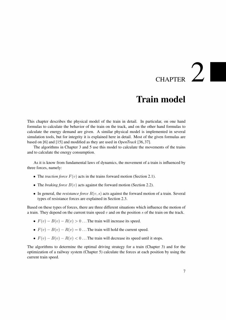
As it is know from fundamental laws of dynamics, the movement of a train is influenced bythree forces, namely:
• The traction force F (v) acts in the trains forward motion (Section 2.1).
• The braking force B(v) acts against the forward motion (Section 2.2).
• In general, the resistance force R(v, s) acts against the forward motion of a train. Severaltypes of resistance forces are explained in Section 2.3.
Based on these types of forces, there are three different situations which influence the motion ofa train. They depend on the current train speed v and on the position s of the train on the track.
• F (v)−B(v)−R(v) > 0 . . . The train will increase its speed.
• F (v)−B(v)−R(v) = 0 . . . The train will hold the current speed.
• F (v)−B(v)−R(v) < 0 . . . The train will decrease its speed until it stops.
The algorithms to determine the optimal driving strategy for a train (Chapter 3) and for theoptimization of a railway system (Chapter 5) calculate the forces at each position by using thecurrent train speed.
7

2.1 Traction force
The traction force of a traction vehicle is given as a table with two columns – the first one is thespeed v in km/h and the second one the corresponding force on the wheels F (v) in kN. Thus,for each speed value v a corresponding traction force value F (v) is defined.
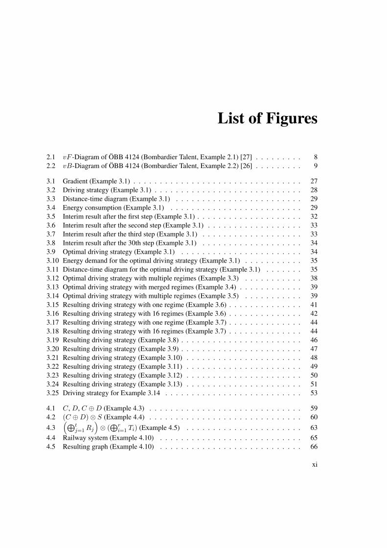
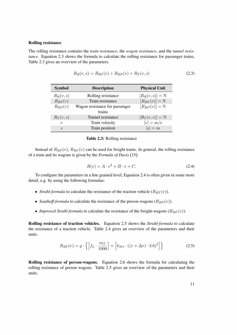
Example 2.1. Figure 2.1 shows the velocity–traction-force diagram of the ÖBB 4124 (Bom-bardier Talent) [27]. The maximum traction effort of the train is located between 0 km/h and47 km/h and is 110.00 kN.
Between 47 km/h and the maximum speed of the train (v = 140 km/h, F (v) = 32.37 kN),there is a nearly continuous traction effort which is inversely proportional to the correspondingspeed value. Thus, the traction force decreases with higher speed values and as a consequencethe acceleration will decrease, too. This effect will be increased by several resistance valueswhich will be explained in section 2.3.
0 20 40 60 80 100 120 1400
10
20
30
40
50
60
70
80
90
100
110
120
Velocity v [km/h]
Trac
tion
forc
eF
(v)
[kN
]
Figure 2.1: vF -Diagram of ÖBB 4124 (Bombardier Talent, Example 2.1) [27]
8

2.2 Braking force
Similarly to the traction force, the braking force is also given as a table with the speed value v inkm/h in the first column and the braking force B(v) in kN in the second one. Again, for eachspeed value v a corresponding braking force B(v) is defined.
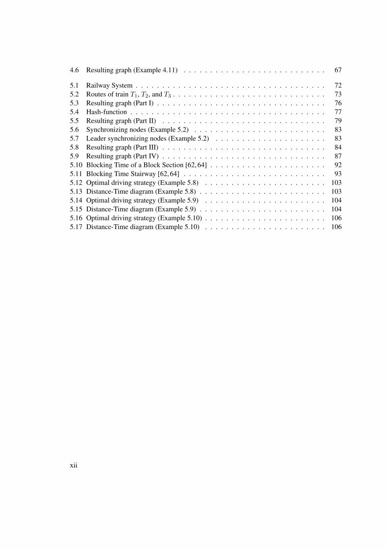
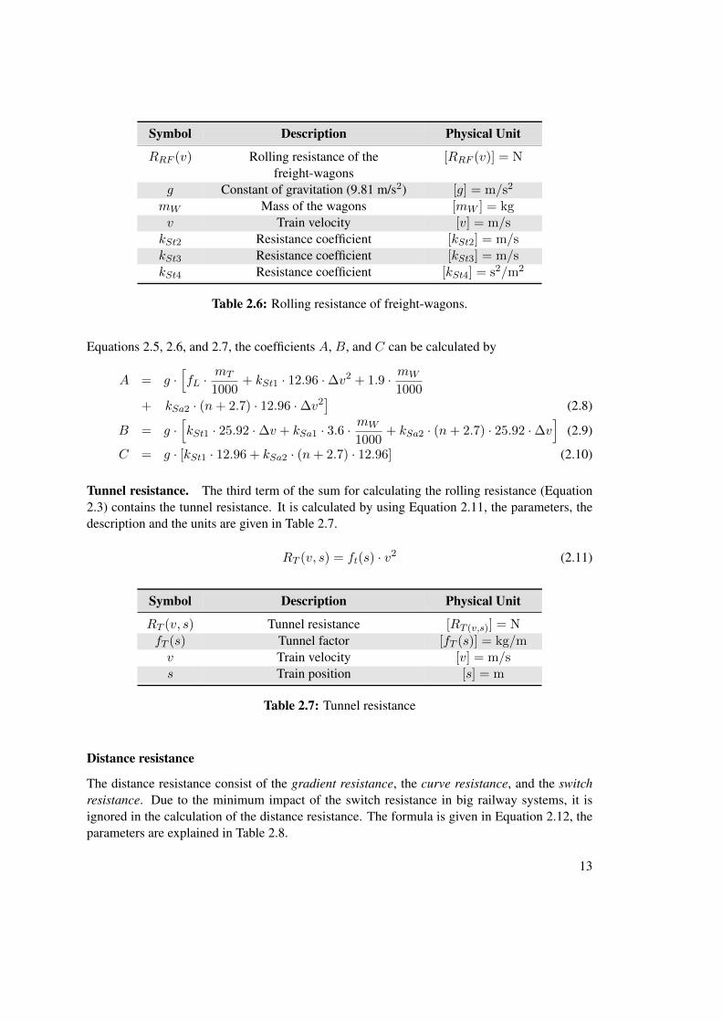
Example 2.2. The velocity–braking-force diagram of ÖBB 4124 (Bombardier Talent) [26] isshown in Figure 2.2. The maximum braking force is located between 0 km/h and 80 km/h andis 80 kN.
Between 80 km/h and the maximum speed of the train (v = 140 km/h, B(v) = 45 kN),there is a decreasing braking power, again inversely proportional to the corresponding speedvalue.
0 20 40 60 80 100 120 1400
10
20
30
40
50
60
70
80
Velocity v [km/h]
Bra
king
forc
eB
(v)
[kN
]
Figure 2.2: vB-Diagram of ÖBB 4124 (Bombardier Talent, Example 2.2) [26]
9
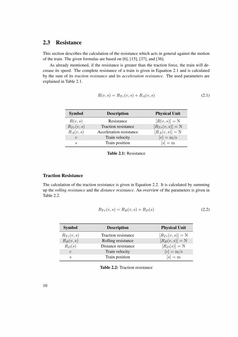
2.3 Resistance
This section describes the calculation of the resistance which acts in general against the motionof the train. The given formulas are based on [6], [15], [37], and [36].
As already mentioned, if the resistance is greater than the traction force, the train will de-crease its speed. The complete resistance of a train is given in Equation 2.1 and is calculatedby the sum of its traction resistance and its acceleration resistance. The used parameters areexplained in Table 2.1.
R(v, s) = RTr(v, s) +RA(v, s) (2.1)
Symbol Description Physical Unit
R(v, s) Resistance [R(v, s)] = NRTr(v, s) Traction resistance [RTr(v, s)] = NRA(v, s) Acceleration resistance [RA(v, s)] = N
v Train velocity [v] = m/ss Train position [s] = m
Table 2.1: Resistance
Traction Resistance
The calculation of the traction resistance is given in Equation 2.2. It is calculated by summingup the rolling resistance and the distance resistance. An overview of the parameters is given inTable 2.2.
RTr(v, s) = RR(v, s) +RD(s) (2.2)
Symbol Description Physical Unit
RTr(v, s) Traction resistance [RTr(v, s)] = NRR(v, s) Rolling resistance [RR(v, s)] = NRD(s) Distance resistance [RD(s)] = Nv Train velocity [v] = m/ss Train position [s] = m
Table 2.2: Traction resistance
10
Rolling resistance
The rolling resistance contains the train resistance, the wagon resistance, and the tunnel resis-tance. Equation 2.3 shows the formula to calculate the rolling resistance for passenger trains,Table 2.3 gives an overview of the parameters.
RR(v, s) = RRT (v) +RRP (v) +RT (v, s) (2.3)
Symbol Description Physical Unit
RR(v, s) Rolling resistance [RR(v, s)] = NRRT (v) Train resistance [RRT (v)] = NRRP (v) Wagon resistance for passenger
trains[RRP (v)] = N
RT (v, s) Tunnel resistance [RT (v, s)] = Nv Train velocity [v] = m/ss Train position [s] = m
Table 2.3: Rolling resistance
Instead of RRP (v), RRF (v) can be used for freight trains. In general, the rolling resistanceof a train and its wagons is given by the Formula of Davis [15]:
R(v) = A · v2 +B · v + C. (2.4)
To configure the parameters in a fine grained level, Equation 2.4 is often given in some moredetail, e.g. by using the following formulas:
• Strahl-formula to calculate the resistance of the traction vehicle (RRT (v)).
• Sauthoff-formula to calculate the resistance of the person-wagons (RRP (v)).
• Improved Strahl-formula to calculate the resistance of the freight-wagons (RRF (v)).
Rolling resistance of traction vehicles. Equation 2.5 shows the Strahl-formula to calculatethe resistance of a traction vehicle. Table 2.4 gives an overview of the parameters and theirunits.
RRT (v) = g ·{[fL ·
mT
1000
]+[kSt1 · ((v + ∆v) · 3.6)2
]}(2.5)
Rolling resistance of person-wagons. Equation 2.6 shows the formula for calculating therolling resistance of person wagons. Table 2.5 gives an overview of the parameters and theirunits.
11

Symbol Description Physical Unit
RRT (v) Rolling resistance of the tractionvehicle
[RRT (v)] = N
g Constant of gravitation (9.81 m/s2) [g] = m/s2
mT Mass of the traction vehicle [mT ] = kgv Train velocity [v] = m/s
∆v Supplement wind speed [∆v] = m/sfL Resistance factor [fL] = 1kSt1 Resistance coefficient [kSt1] = kg ·s2/m2
Table 2.4: Rolling resistance of the traction vehicle
RRP (v) = g ·{[
1.9 · mW
1000
]+[kSa1 · v · 3.6 ·
mW
1000
]+[kSa2 · (n+ 2.7) · ((v + ∆v) · 3.6)2
]} (2.6)
Symbol Description Physical Unit
RRP (v) Rolling resistance of theperson-wagons
[RRP (v)] = N
g Constant of gravitation [g] = m/s2
mW Mass of the wagons [mW ] = kgn Number of wagons [n] = 1v Train velocity [v] = m/s
∆v Supplement wind speed [∆v] = m/skSa1 Resistance coefficient [kSa1] = s/mkSa2 Resistance coefficient [kSa2] = kg·s2/m2
Table 2.5: Rolling resistance of person-wagons.
Rolling resistance of freight-wagons. Equation 2.7 shows the formula for calculating therolling resistance of freight wagons. Table 2.6 gives an overview of the parameters and theirunits.
RRF (v) = g · m
1000·[2.2− kSt2
v · 3.6 + kSt3+ kSt4 · (v · 3.6)2
](2.7)
As already mentioned (Equation 2.4), the resistance of the traction vehicle and the wagonsis often given by the Formula of Davis. Based on Equation 2.4, by summing up all terms of
12
Symbol Description Physical Unit
RRF (v) Rolling resistance of thefreight-wagons
[RRF (v)] = N
g Constant of gravitation (9.81 m/s2) [g] = m/s2
mW Mass of the wagons [mW ] = kgv Train velocity [v] = m/skSt2 Resistance coefficient [kSt2] = m/skSt3 Resistance coefficient [kSt3] = m/skSt4 Resistance coefficient [kSt4] = s2/m2
Table 2.6: Rolling resistance of freight-wagons.
Equations 2.5, 2.6, and 2.7, the coefficients A, B, and C can be calculated by
A = g ·[fL ·
mT
1000+ kSt1 · 12.96 ·∆v2 + 1.9 · mW
1000+ kSa2 · (n+ 2.7) · 12.96 ·∆v2
](2.8)
B = g ·[kSt1 · 25.92 ·∆v + kSa1 · 3.6 ·
mW
1000+ kSa2 · (n+ 2.7) · 25.92 ·∆v
](2.9)
C = g · [kSt1 · 12.96 + kSa2 · (n+ 2.7) · 12.96] (2.10)
Tunnel resistance. The third term of the sum for calculating the rolling resistance (Equation2.3) contains the tunnel resistance. It is calculated by using Equation 2.11, the parameters, thedescription and the units are given in Table 2.7.
RT (v, s) = ft(s) · v2 (2.11)
Symbol Description Physical Unit
RT (v, s) Tunnel resistance [RT (v,s)] = N
fT (s) Tunnel factor [fT (s)] = kg/mv Train velocity [v] = m/ss Train position [s] = m
Table 2.7: Tunnel resistance
Distance resistance
The distance resistance consist of the gradient resistance, the curve resistance, and the switchresistance. Due to the minimum impact of the switch resistance in big railway systems, it isignored in the calculation of the distance resistance. The formula is given in Equation 2.12, theparameters are explained in Table 2.8.
13

RD(s) = RG(s) +RC(s) +RS(s) (2.12)
Symbol Description Physical Unit
RD(s) Distance resistance [RD(s)] = NRG(s) Gradient resistance [RG(s)] = NRC(s) Curve resistance [RC(s)] = NRS(s) Switch resistance [RS(s)] = Ns Train position [s] = m
Table 2.8: Distance resistance
Gradient resistance. The gradient resistance is calculated by
RG(s) = m · g · sin (α(s)) (2.13)
For small inclination α(s), sinα(s) can be substituted by tan (α(s)):
RG(s) = m · g · tan (α(s)) = m · g · I(s)
1000(2.14)
The used parameters are explained in Table 2.9.
Symbol Description Physical Unit
RG(s) Gradient resistance [RG(s)] = Nα(s) Inclination at position s [α(s)] =◦
g Constant of gravitation (9.81 m/s2) [g] = m/s2
m Complete mass of the train(mT +mW )
[m] = kg
I(s) Track Gradient at position s [I(s)] = hs Train position [s] = m
Table 2.9: Gradient resistance
Curve resistance. The curve resistance for a curve radius r ≥ 300 m is calculated by
RC(s) =6.3
r(s)− 55·m (2.15)
and for r(s) < 300 m by
RC(s) =4.91
r(s)− 30·m. (2.16)
The parameters are explained in Table 2.10.
14
Symbol Description Physical Unit
RC(s) Curve resistance [RC(s)] = Nr(s) Curve radius [r(s)] = mm Complete mass of the train
(mT +mW )[m] = kg
s Train position [s] = m
Table 2.10: Curve resistance
Acceleration Resistance
While the train is accelerating or decelerating, the so called acceleration resistance acts on thetrain (Equation 2.17).
RA(v, s) = m · a(v, s) · (1 + 0.01 · ρ) (2.17)
The parameters of Equation 2.17 are explained in Table 2.11.
Symbol Description Physical Unit
RA(v, s) Acceleration resistance [RA(v, s)] = Nm Complete mass of the train
(mT +mW )[m] = kg
a(v, s) Acceleration [a(v, s)] = m/s2
ρ Rotating mass factor [ρ] = 1v Train velocity [v] = m/ss Train position [s] = m
Table 2.11: Acceleration resistance
As a result, the complete resistance for a person train is calculated by
R(v, s) = RRT (v) +RRP (v) +RT (v, s) +RG(s) +RC(s) +RS(s) +RA(v, s) (2.18)
and for a freight train by
R(v, s) = RRT (v) +RRF (v) +RT (v, s) +RG(s) +RC(s) +RS(s) +RA(v, s) (2.19)
and by using the Formula of Davis
R(v, s) = A · v2 +B · v + C +RT (v, s) +RG(s) +RC(s) +RS(s) +RA(v, s) (2.20)
whereby A, B, and C depends on the train type (passenger or freight train) and its charac-teristics.
15
2.4 Train Dynamics
This section describes the calculation of the acceleration value a(v, s) for a train accelerating,braking, and coasting. Additionally, formulas for speed-holding and the calculation of the cur-rent speed value and the travel time of a train are given. The formulas are based on the equationsof the previous section (Equations 2.1 - 2.20). To calculate the motion of a train, it is neces-sary to know the traction force F (v), the braking force B(v) and the resistance values R(v, s).Based on these parameters, it can be determined if the train accelerates, holds its speed, or de-celerates. In the following, it is assumed that for both, traction force and braking force, themaximum force will be used. This approach is used typically in the field and has mathematicaland physical reasons.
Acceleration
Assuming that the driver will use maximum traction force (F (v) > 0 N) – and thus no brakingforce (B(v) = 0 N) – the acceleration value for passenger trains is be calculated by:
a(v, s) =F (v)− (RRT (v) +RRP (v) +RT (v, s))− (RG(s) +RC(s) +RS(s))
m · (1 + 0.01 · ρ)(2.21)
As already mentioned, the resistance parameters depend on various factors, e.g. the trainmass, the current speed, or the inclination of the track. Based on Equation 2.21, the followingthree different kinds of situations can happen:
• The train will increase its speed if
F (v) > RRT (v) +RRP (v) +RRP (v) +RG(s) +RC(s) +RS(s).
• The train will hold its speed if
F (v) = RRT (v) +RRP (v) +RRP (v) +RG(s) +RC(s) +RS(s).
• The train will decrease its speed if
F (v) < RRT (v) +RRP (v) +RRP (v) +RG(s) +RC(s) +RS(s).
Deceleration
Assuming that the driver will use the maximum braking power (B(v) > 0 N) – and thus notraction force is available (F (v) = 0 N) – the deceleration value for passenger trains is calculatedby:
a(v, s) = −[B(v) +RRT (v) +RRP (v) +RT (v) +RG(s) +RC(s) +RS(s)
m · (1 + 0.01 · ρ)
](2.22)
Similar to the acceleration, again three different kinds of situation can occur:
16
• The train will decrease its speed if
B(v) > RRT (v) +RRP (v) +RRP (v) +RG(s) +RC(s) +RS(s).
• The train will hold its speed if
B(v) = RRT (v) +RRP (v) +RRP (v) +RG(s) +RC(s) +RS(s).
• The train will increase its speed if
B(v) < RRT (v) +RRP (v) +RRP (v) +RG(s) +RC(s) +RS(s).
Coasting
Assuming that the train driver neither uses its traction force nor its acceleration force. As aconsequence, the train is in its so-called coasting phase. In that case only the resistance valuesinfluence the motion of the train. Equation 2.23 shows the formula for calculating the accelera-tion value of a passenger train.
a(v, s) = −[RRT (v) +RRP (v) +RT (v) +RG(s) +RC(s) +RS(s)
m · (1 + 0.01 · ρ)
](2.23)
Again, three different situation can happen, based on the resistance parameters:
• The train will decrease its speed
−RG(s) < RRT (v) +RRP (v) +RT (v) +RC(s) +RS(s)
• The train will hold its speed
−RG(s) = RRT (v) +RRP (v) +RT (v) +RC(s) +RS(s)
• The train will increase its speed if
−RG(s) > RRT (v) +RRP (v) +RT (v) +RC(s) +RS(s)
Speed-holding
To hold the current speed value the parameters acting in the direction of the trains motion andthe parameters against the motion must be in equality:
F (v)−B(v)− (RRT (v) +RRP (v) +RRP (v))− (RG(s) +RC(s) +RS(s)) = 0. (2.24)
17

Symbol Description Physical Unit
s Travel distance [s] = ms0 Starting position [s0] = mt Travel time [t] = s
a(v0, s0) Acceleration value [a(v0, s0)] = m/s2
v0 Starting speed value [v0] = m/s
Table 2.12: Calculation of the speed value
Calculation of the speed value
After the calculation of the acceleration value for a given speed and a given position, the speedvalue of the next position can be determined by
s = s0 + v0 · t+1
2· a(v0, s0) · t2. (2.25)
where v0 is the current speed and ans s0 the current position. The parameters of Equation 2.25are explained in Table 2.12.
Calculation of the travel time
If a starting position s0, the driving distance d, the initial speed v0, and the acceleration valuea are known, the required travel time t and the speed value v for a driving distance d can becalculated by
v = v0 + ∆v = v0 + a(v0, s0) · t. (2.26)
These formulas can be used for a train accelerating (a(v0, s0) > 0 m/s2), decelerating(a(v0, s0) < 0 m/s2), and speed holding (a(v0, s0) = 0 m/s2). By using the numerical in-tegration with a step size of s = 1 m, the resulting speed v and travel time t after distance d canbe calculated.
2.5 Energy consumption
As it is know from fundamental physical laws (cf. [2]) the overall energy consumption can becalculated by integrating the resulting force F (v, s) = F (v)−B(v)−R(v, s) over the covereddistance s:
E(s) =
∫F (v, s)ds (2.27)
Parameters of Equation 2.27 are explained in Table 2.13.By using numerical integration with a step size of 1 m the following three kinds of situations
are possible:
18
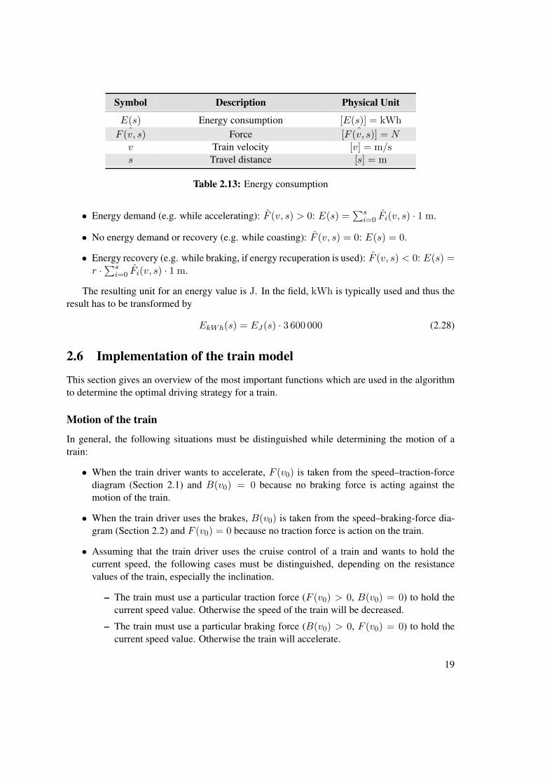
Symbol Description Physical Unit
E(s) Energy consumption [E(s)] = kWhˆF (v, s) Force [ ˆF (v, s)] = Nv Train velocity [v] = m/ss Travel distance [s] = m
Table 2.13: Energy consumption
• Energy demand (e.g. while accelerating): F (v, s) > 0: E(s) =∑s
i=0 Fi(v, s) · 1 m.
• No energy demand or recovery (e.g. while coasting): F (v, s) = 0: E(s) = 0.
• Energy recovery (e.g. while braking, if energy recuperation is used): F (v, s) < 0: E(s) =r ·∑s
i=0 Fi(v, s) · 1 m.
The resulting unit for an energy value is J. In the field, kWh is typically used and thus theresult has to be transformed by
EkWh(s) = EJ(s) · 3 600 000 (2.28)
2.6 Implementation of the train model
This section gives an overview of the most important functions which are used in the algorithmto determine the optimal driving strategy for a train.
Motion of the train
In general, the following situations must be distinguished while determining the motion of atrain:
• When the train driver wants to accelerate, F (v0) is taken from the speed–traction-forcediagram (Section 2.1) and B(v0) = 0 because no braking force is acting against themotion of the train.
• When the train driver uses the brakes, B(v0) is taken from the speed–braking-force dia-gram (Section 2.2) and F (v0) = 0 because no traction force is action on the train.
• Assuming that the train driver uses the cruise control of a train and wants to hold thecurrent speed, the following cases must be distinguished, depending on the resistancevalues of the train, especially the inclination.
– The train must use a particular traction force (F (v0) > 0, B(v0) = 0) to hold thecurrent speed value. Otherwise the speed of the train will be decreased.
– The train must use a particular braking force (B(v0) > 0, F (v0) = 0) to hold thecurrent speed value. Otherwise the train will accelerate.
19

– No additional force will be applied to the motion of the train (F (v0) = 0, B(v0) =0).
Algorithm 2.1: trainMotion (Calculate the motion of a train)input : v0,s0,t0,e0output: v, s, t, e
1 a← getAcceleration(v0, s0);2 (v, t, s)← calcSpeed(v0, t0, s0, a);3 e← e0 + calcEnergy(v, s);4 return (v, t, s, e);
Depending on the above restrictions Algorithm 2.1 calculates the motion of the train. Inparticular, the resulting speed value v, the resulting travel time t and the new position s aredetermined by assuming that the train starts at position s0 with a given speed value v0 at a giveninstant of time t0 and drives exactly 1 m. Based on the current speed value, the position, theapplied traction force F (v0) and braking force B(v0) the acceleration value a and the energyconsumption e for the trip are calculated.
Example 2.3. Assume that a train starts at a railway station at position s0 = 1 000 m withv0 = 0 km/h and accelerates until position s1 = 1 400 m is reached. The train starts itsjourney at t0 = 0 s. Now Algorithm 2.1 is used in a loop.
Algorithm 2.2: Algorithm of Example 2.31 v0 ← 0 km/h;2 s0 ← 1 000 m;3 s1 ← 1 400 m;4 t0 ← 0 s;5 e0 ← 0 kWh;
6 s← s0;7 v ← v0;8 t← t0;9 e← e0;
10 while s < s1 do11 (v, s, t, e)← trainMotion(v, s, t, e);12 end
By applying Algorithm 2.2 the train finally reaches position s = s1. The speed value v holdsthe speed at this position, t contains the travel time and e the energy consumption.
Determining the speed change of a train
As already mentioned the acceleration of deceleration and thus the train speed depends on sev-eral parameters, in particular on the traction force F (v0), the braking force B(v0) and the resis-
20
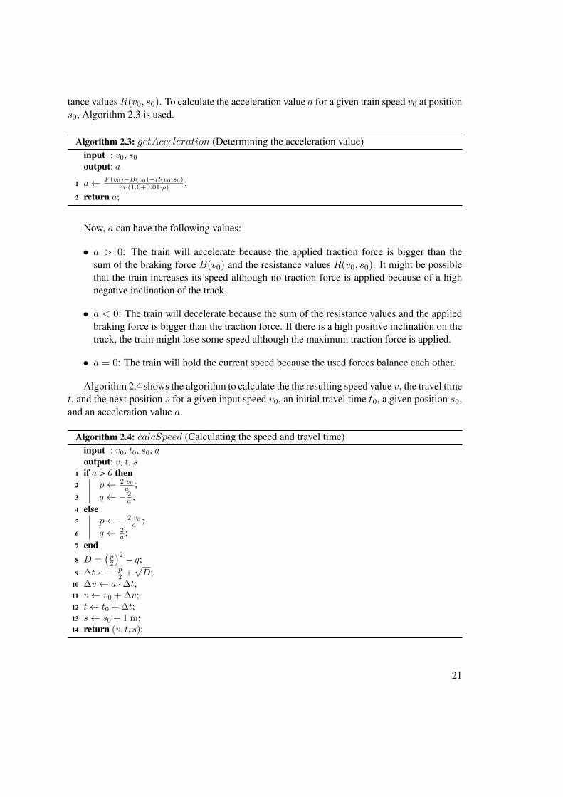
tance valuesR(v0, s0). To calculate the acceleration value a for a given train speed v0 at positions0, Algorithm 2.3 is used.
Algorithm 2.3: getAcceleration (Determining the acceleration value)input : v0, s0output: a
1 a← F (v0)−B(v0)−R(v0,s0)m·(1.0+0.01·ρ) ;
2 return a;
Now, a can have the following values:
• a > 0: The train will accelerate because the applied traction force is bigger than thesum of the braking force B(v0) and the resistance values R(v0, s0). It might be possiblethat the train increases its speed although no traction force is applied because of a highnegative inclination of the track.
• a < 0: The train will decelerate because the sum of the resistance values and the appliedbraking force is bigger than the traction force. If there is a high positive inclination on thetrack, the train might lose some speed although the maximum traction force is applied.
• a = 0: The train will hold the current speed because the used forces balance each other.
Algorithm 2.4 shows the algorithm to calculate the the resulting speed value v, the travel timet, and the next position s for a given input speed v0, an initial travel time t0, a given position s0,and an acceleration value a.
Algorithm 2.4: calcSpeed (Calculating the speed and travel time)input : v0, t0, s0, aoutput: v, t, s
1 if a > 0 then2 p← 2·v0
a ;3 q ← − 2
a ;4 else5 p← − 2·v0
a ;6 q ← 2
a ;7 end8 D =
(p2
)2 − q;9 ∆t← −p2 +
√D;
10 ∆v ← a ·∆t;11 v ← v0 + ∆v;12 t← t0 + ∆t;13 s← s0 + 1 m;14 return (v, t, s);
21

Calculating the energy consumption
Equation 2.27 from Section 2.5 is used to calculate the energy consumption of a train. Algo-rithm 2.5 describes the algorithm for the calculation, where getResistance(v, a, s) calculatesthe complete resistance as described in Section 2.3.
Algorithm 2.5: calcEnergy (Calculate the energy consumption of a train)input : v, soutput: e
1 r ← getResistance(v, s);2 e← e+ r · 3 000 000;3 return e;
Now, the train model is explained in detail and an overview about the implementation isgiven. The next chapter explains the algorithm to find the optimal driving strategy of a train,based on the restrictions of this chapter.
Further examples showing the impact of the train parameters and the track parameters aregiven in Section 3.6.
22
CHAPTER 3Single trip optimization
3.1 Introduction
As already discussed in several scientific publications, there exist a lot of algorithms to find theoptimal driving strategy for the journey of a single train, which cannot be used for real-time-applications, because of practical restrictions (e.g. Chapter 1) like computation time, passengercomfort or drive-ability.
In general, the optimal driving strategy depends on various factors of influence, e.g.
• the gradient of the track and speed restrictions,
• the length and weight of the train,
• the scheduled travel time,
• traction power and braking capability,
• recuperation behavior, and
• various resistance parameters.
It is know from several publications (cf. [2, 46]) that the optimal driving strategy for a train,which starts at a given position ss and drives within a given travel time t on a specified track toreach its destination (final position) sf , may contain the following driving modes in exactly thisorder:
1. Acceleration-phase. The train starts its acceleration-phase with maximum traction forceat the start position ss with a given starting speed vs (e.g. 0 km/h at a railway station)and accelerates until the hold speed vh and the hold position sh are reached. The resultingtravel time for this phase is ta.
23

2. Speed-hold-phase. The train starts its speed-hold-phase at the hold position sh with holdspeed vh and drives with constant speed until the coasting position sc is reached. Thespeed value at this position is called coasting speed vc and is equal to vh. The travel timefor the hold phase is th.
3. Coasting-phase. The coasting-phase starts at the coasting position sc and ends at thebraking position sb. During this phase, the train will not use its traction or braking force.It will just roll until the braking position is reached. The travel time of this phase is tc.
4. Braking-phase. The braking-phase starts at the braking position sb and ends at the finalposition sf . The speed decreases from vb to vf (e.g. to 0 km/h at a commercial stopwhich can be station or stop). The required travel time for the braking-phase is tb.
The speed values above are limited by the maximum train speed and the track speed limit.Usually, the start position ss, the corresponding speed vs, the final position sf , and the finalspeed value vf of a trip are known. Thus the challenge is to determine the other three tuples(sh, vh), (sc, vc), (sb, vb) with respect to the following restriction:
• A train Tk must reach its destination within the planned travel time tk�
.
• The driving-comfort for passengers (e.g. there should be a minimum of transitions be-tween the driving types) and the driver (e.g. each driving type should last at least a givenduration in seconds) must be ensured .
• The energy consumption must be minimal. It is calculated by e = ed − er where e is theenergy consumption, ed is the energy demand, and er is the energy recovery of the trip.
• The result must be available as fast as possible to use the algorithm for online-systems.
Definition 3.1 (Maximum train speed). The maximum speed of train k, based on the train char-acteristics (Chapter 2), is denoted by vk.
Definition 3.2 (Maximum allowed track speed). The maximum allowed speed on track sectioni is denoted by vi.
Definition 3.3 (Maximum speed). The maximum allowed speed v is defined as v = min(vk, vi
).
Definition 3.4 (Regime). A part of the track with constant maximum speed is called a regime.
As a consequence, a track with constant track speed consists of exactly one regime. Thedefinition of regime can be extended:
Definition 3.5 (Regime (extended)). A part of the track with constant maximum and no (signif-icant) gradient changes is called a regime.
The following sections describe the algorithm to find the optimal driving strategy for a singletrain with no interaction to other trains. The explanation starts with a track, consisting of a singleregime and will be extended to a multi-regime optimization.
24

3.2 Simple Algorithm
This section describes the algorithm to find the optimal driving strategy for a train with a givenmaximum speed along the complete track and thus, with only one regime, based on the previ-ously mentioned restrictions. A train k starts at a railway station with vs = 0 km/h and shouldarrive at another railway station after the planned travel time tk
�. Thus, vf = 0 km/h.
The following algorithm is very efficient in terms of calculation time and can be adjusted byseveral parameters. The first part of the algorithm consists of finding a driving strategy consistingof
• acceleration-phase,
• speed-hold-phase, and
• braking-phase.
To get a valid driving strategy the following equation must be fulfilled:
tk�≈ tka + tkh + tkb (3.1)
In general, it is hard to find a driving strategy where the left side of Equation 3.1 conformsexactly the planned travel time. Thus, a result is valid, if it is within a slight time interval aroundtk�
and for this reason the ≈-operator is used.Due to the fact that the speed values at the beginning vs and at the end vf of the journey
are known and assuming that the maximum force is used for the acceleration and braking-phase,only the hold speed vh must be determined. This is done by using a binary search algorithm.
Algorithm
Algorithm 3.1 determines the driving strategy and works as follows:
• If the planned travel time tk�
for train k is less than the shortest travel time (maybe alsorunning time), no solution can be found.
• Otherwise, the algorithm loops until an appropriate solution (tk�≈ tka + tkh + tkb ) is found:
– Calculate a new hold speed vh = v+v2 , where v is the lower boundary speed value1
and v is the upper boundary speed value.
– The train starts at sh and accelerates until the hold speed vh is reached.
– Calculate the braking position for vh2.
– Hold the current speed, starting at the hold position sh until the braking position sbis reached.
1v is set to a value slightly greater than 0 km/h initially.2When the train starts braking at the braking position (with maximum braking force), it will decrease its speed
until it stops at the final position.
25

– Brake until the final position sf is reached.
– Calculate the complete travel time t.
– If an appropriate solution (tk�≈ tka + tkh + tkb ) is found, calculate the energy con-
sumption for this driving strategy.
– If no solution is found, the upper boundary speed value or the lower boundary speedvalue is changed:
∗ v = vh, if t < tk�
∗ v = vh, if t > tk�
Algorithm 3.1: calcHoldSpeed (Algorithm to calculate the hold speed)input : ss, sf , tk
�, v
output: sh, sb, vh, vb, e
1 not_finished← true;2 v← 0;
3 while not_finished do4 vh ← (v + v) / 2;
5 (sh,ta,ea)← Accelerate(ss,vh);6 (sb,tb)← GetBrakingPosition(sf vh);7 (th,eh)← SpeedHold(sh,sb,vh);8 (tb,eb)← Brake(sb,sf);
9 t← ta +th +tb;
10 if t ≈ tk�
then11 not_finished← false;12 e← ea +eh +eb;13 vb← vh;14 else15 if t < tk
�then
16 v← vh;17 else18 v← vh;19 end20 end
21 return (sh,sb,vh,vb,e);22 end
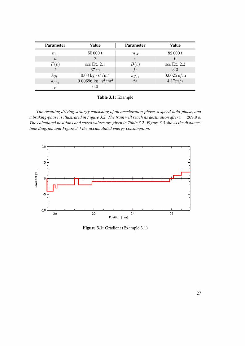
Example 3.1. In the following example, the hold-strategy for a single train is calculated. Itsjourney starts at ss = 19 584 m and ends at sf = 26 955 m. The planned travel time istk�
= 270 s. The train-specific parameters can be found in Table 3.1 and the track gradientis illustrated in Figure 3.1.
26
Parameter Value Parameter Value
mT 55 000 t mW 82 000 tn 2 r 0
F (v) see Ex. 2.1 B(v) see Ex. 2.2l 67 m fL 3.3
kSt1 0.03 kg · s2/m2 kSa1 0.0025 s/mkSa2 0.00696 kg · s2/m2 ∆v 4.17m/sρ 6.0
Table 3.1: Example
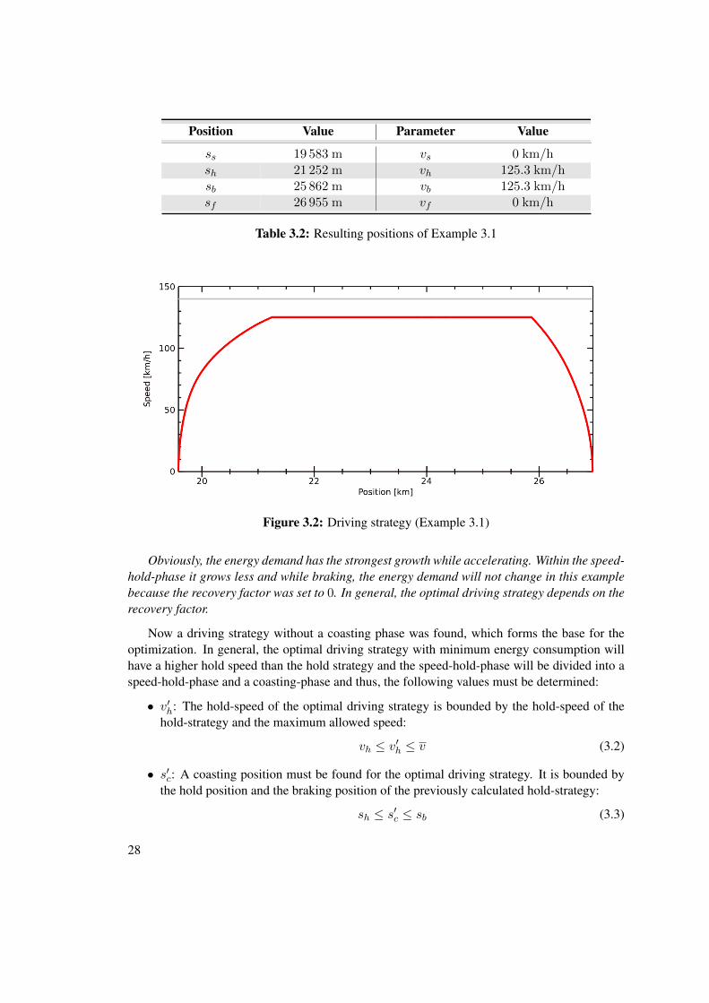
The resulting driving strategy consisting of an acceleration-phase, a speed-hold-phase, anda braking-phase is illustrated in Figure 3.2. The train will reach its destination after t = 269.9 s.The calculated positions and speed values are given in Table 3.2. Figure 3.3 shows the distance-time diagram and Figure 3.4 the accumulated energy consumption.
Figure 3.1: Gradient (Example 3.1)
27
Position Value Parameter Value
ss 19 583 m vs 0 km/hsh 21 252 m vh 125.3 km/hsb 25 862 m vb 125.3 km/hsf 26 955 m vf 0 km/h
Table 3.2: Resulting positions of Example 3.1
Figure 3.2: Driving strategy (Example 3.1)
Obviously, the energy demand has the strongest growth while accelerating. Within the speed-hold-phase it grows less and while braking, the energy demand will not change in this examplebecause the recovery factor was set to 0. In general, the optimal driving strategy depends on therecovery factor.
Now a driving strategy without a coasting phase was found, which forms the base for theoptimization. In general, the optimal driving strategy with minimum energy consumption willhave a higher hold speed than the hold strategy and the speed-hold-phase will be divided into aspeed-hold-phase and a coasting-phase and thus, the following values must be determined:
• v′h: The hold-speed of the optimal driving strategy is bounded by the hold-speed of thehold-strategy and the maximum allowed speed:
vh ≤ v′h ≤ v (3.2)
• s′c: A coasting position must be found for the optimal driving strategy. It is bounded bythe hold position and the braking position of the previously calculated hold-strategy:
sh ≤ s′c ≤ sb (3.3)
28

Figure 3.3: Distance-time diagram (Example 3.1)
Figure 3.4: Energy consumption (Example 3.1)
• Based on these two values, the other speed values and positions will be determined.
As a result, the challenge is to find the hold-speed v′h and the coasting position s′c in a way that theenergy consumption is as small as possible. Assuming that vh = 80 km/h and v = 140 km/h,the hold-speed for the optimal driving strategy will be 80 km/h ≤ v′h ≤ 140 km/h. Due to thegradient values, it is not possible to use a binary search algorithm to find the best speed value andthus, every value in this range might be the best solution. Due to restrictions on the calculation
29

time, a parameter to the algorithm is introduced to adjust the step size within the range: v+. As aresult, the following hold-speed values will be used for the determination of the optimal drivingstrategy:
vh, vh + v+, vh + 2 · v+, vh + 3 · v+ . . . v
When using v+ = 5 km/h, the following hold-speed values will be used for further calcu-lations:
80 km/h, 85 km/h, 90 km/h, 95 km/h, 100 km/h, 105 km/h, 110 km/h,115 km/h, 120 km/h, 125 km/h, 130 km/h, 135 km/h, 140 km/h
Due to the fact that some cruise control systems of the trains can be adjusted only in 5-km/h-steps, this parameter can be used to set-up the algorithm in a way that the computedresults can be used in practice. Based on this parameter, the hold speed must be adjusted in away that it is a whole-number multiple of the v+ and less or equal to the calculated value fromthe hold-strategy:
vh ≤ x · v+ (3.4)
with
x =
⌊vhv+
⌋(3.5)
and thus, the following speed-values will be used for the determination of the optimal drivingstrategy:
vh, vh + v+, vh + 2 · v+, vh + 3 · v+, . . . , v
Assuming that the previously calculated hold speed is vh = 63.56 km/h and v+ = 10 km/h,the modified hold-speed is set to vh = 60 km/h.
Similar to this parameter, a second parameter is available to set-up the granularity for findingthe optimal coasting position: s+. Here, too, the position cannot be found by a binary searchalgorithm because of the track gradient. Assume a hold position sh = 1 000 m and a brakingposition sb = 5 000 m. As a consequence, there is a range of 4 000 m to find the coastingposition. By using s+, designated positions are used for the calculation of the driving strategy:
sh, sh + s+, sh + 2 · s+, sh + 3 · s+, . . . , sb
With decreasing v+ and decreasing s+ the algorithm will find better results in terms ofenergy consumption, but the execution time will increase. For online-systems, it is important tofind a good trade-off between a good result, the execution time, and the practical feasibility.
Algorithm
As already mentioned the hold-strategy forms the basis for the optimization. Initially the mini-mum energy consumption is set to e = ∞. The algorithm starts by calculating the accelerationcurve, starting with the initial speed vs until vh is reached (see Equation 3.4). Next, the brakingcurve for this speed value is calculated in a way that the train arrives at its final position withits final speed vf . If the final position is a stop (e.g. at a railway station), the final speed is set
30
to vf = 0 km/h. The coasting position is set to the braking position and the train will hold itsspeed value until the coasting position is reached. As a result the first calculated driving strat-egy contains the acceleration phase, the speed-hold phase and the braking phase. Based on thefollowing equations, the travel time t and energy consumption e are calculated.
t = ta + th + tc + tb (3.6)
e = ea + eh + ec + eb (3.7)
If the following equations are valid, a new driving strategy with a minimum in terms of energyconsumption has been found:
t ≈ tk�
(3.8)
e < e (3.9)
If a new solution is found, the so far minimum energy consumption will be set to e = e. Next,the coasting position will be decreased by s+ and thus the new driving strategy starts with theacceleration-phase until the maximum speed value is reached, then there is the speed-hold-phaseuntil the coasting position is reached, followed by a coasting-phase until the braking curve isreached. Finally the train will brake until it reaches its the final position. Again, if Equations 3.8and 3.9 are valid, a new minimum is found.
The coasting position is again decreased by s+ and the calculated values are checked. Thisprocedure is repeated until at least one of the following termination conditions are valid:
• The coasting position is equal to the hold position (Equation 3.10) and thus the drivingstrategy contains the acceleration-phase, the coasting-phase, and the braking-phase. Nofurther decrease of the coasting position is possible.
sc = sh (3.10)
• The calculated travel time for the driving strategy is greater than the planned travel time(Equation 3.11). All further driving strategies with the same maximum speed value willhave a higher travel time, because the hold phase decreases and the coasting phase in-creases. This assumption is valid only if the train decelerates or holds its speed whilecoasting.
tk > tk�
(3.11)
• The speed value after the coasting phase is smaller than the final speed (Equation 3.12).This means that the train will not be able to reach its destination with the defined finalspeed value. For instance, a train would stop at the track before it reaches the railwaystation.
vc ≤ vf (3.12)
When there are no further valid solutions for the given hold speed, it is increased by v+, thebraking curve for the new speed is calculated and the braking position is determined. Then theprocedure to find a new solution for the coasting positions starts. The algorithm is finished, if
31
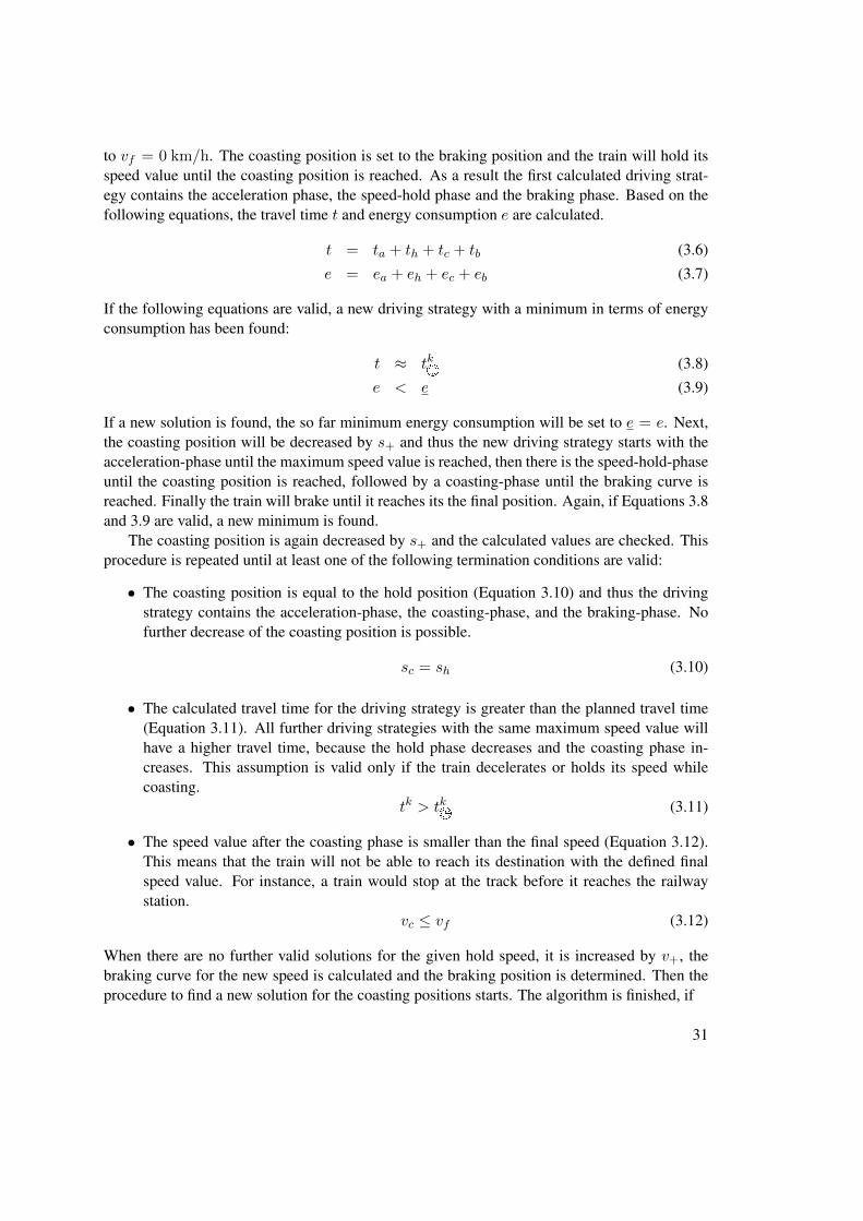
Figure 3.5: Interim result after the first step (Example 3.1)
• the maximum allowed speed is reached (vh = v) and the coasting position cannot befurther decreased (sc = sh) or
• the maximum allowed speed is not reached (vh < v), but the calculated travel time isgreater than the planned travel time (tk > tk
�) and the coasting position cannot be further
decreased (sc = sh).
An optimal driving strategy is found if appropriate speed values and positions are found bythe algorithm. Otherwise, either the planned travel time tk
�cannot be achieved or the algorithm
parameters must be adjusted to a finer grain (e.g. v+ = 5 km/h instead of v+ = 20 km/h ors+ = 10 m instead of s+ = 1000 m).
To avoid several calculations of the acceleration curve and the braking curve, the calculationis done only once and stored in an array, including the energy consumption and the travel timefor each positions. Thus, the required travel time and energy consumption can be reused fordifferent driving strategies. A similar approach is employed for the speed-hold-phase, with therestriction that the calculation must be done for each hold speed, but only once. As a result,the travel time and the energy consumption, again, can be reused for each combination of thespeed-hold-phase and the coasting phase.
Figures 3.5–3.8 show the interim result for Example 3.1 after the first, the second, the third,and the thirtieth step of the algorithm, when using s+ = 100 m. Figures 3.9, 3.10, and 3.11show the results of the optimal driving strategy, where the red line illustrates the hold strategyand the blue one the optimal driving strategy. The results show the distance-speed diagram, theaccumulated energy consumption, and the distance-time diagram.
32

Algorithm 3.2 describes the algorithm to find the optimal driving strategy.
Figure 3.6: Interim result after the second step (Example 3.1)
Figure 3.7: Interim result after the third step (Example 3.1)
Example 3.2. In this example, a train using the hold-strategy consumes 42.386 kWh and whenusing the optimal driving strategy, it consumes 37.908 kWh. In comparison to the hold strategy,the optimal driving strategy will save 4.478 kWh, which is about 11.8 %.
33
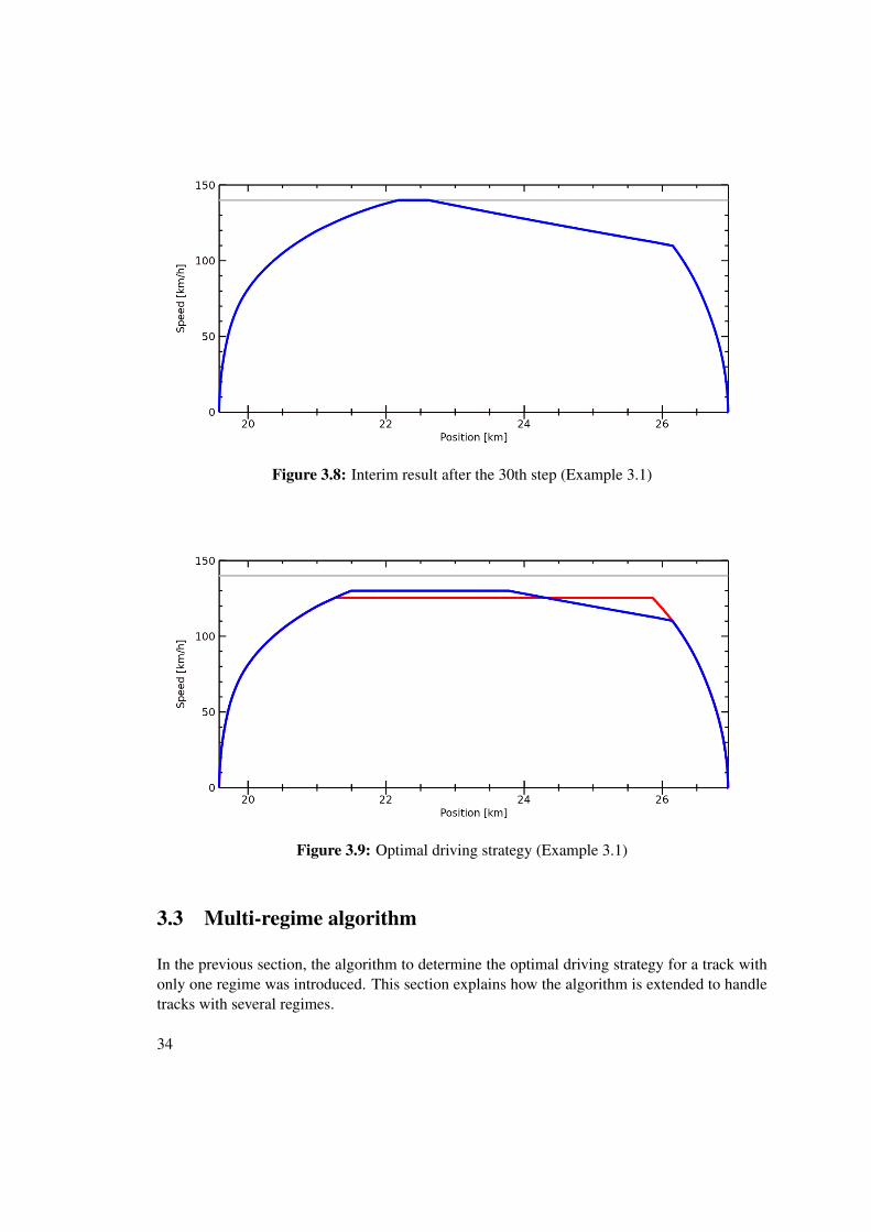
Figure 3.8: Interim result after the 30th step (Example 3.1)
Figure 3.9: Optimal driving strategy (Example 3.1)
3.3 Multi-regime algorithm
In the previous section, the algorithm to determine the optimal driving strategy for a track withonly one regime was introduced. This section explains how the algorithm is extended to handletracks with several regimes.
34
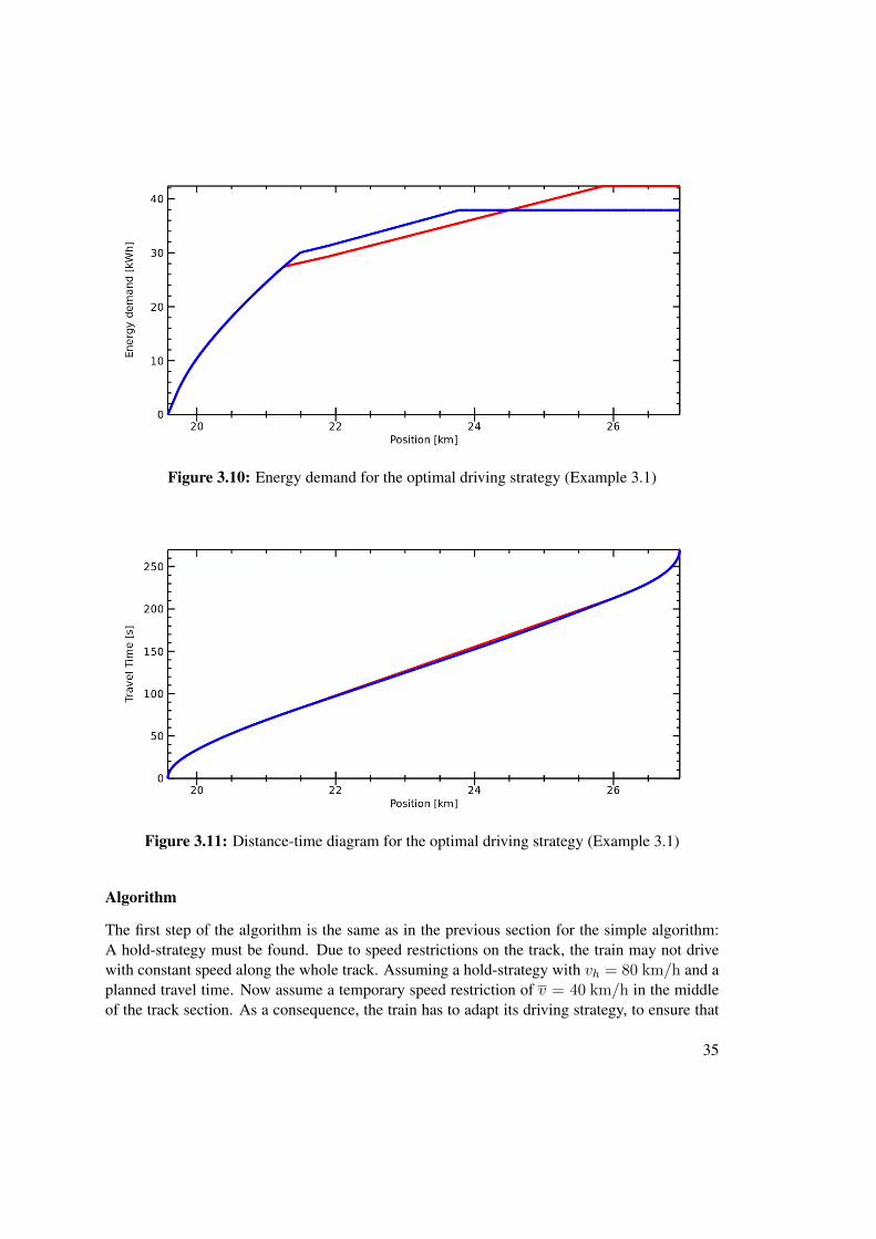
Figure 3.10: Energy demand for the optimal driving strategy (Example 3.1)
Figure 3.11: Distance-time diagram for the optimal driving strategy (Example 3.1)
Algorithm
The first step of the algorithm is the same as in the previous section for the simple algorithm:A hold-strategy must be found. Due to speed restrictions on the track, the train may not drivewith constant speed along the whole track. Assuming a hold-strategy with vh = 80 km/h and aplanned travel time. Now assume a temporary speed restriction of v = 40 km/h in the middleof the track section. As a consequence, the train has to adapt its driving strategy, to ensure that
35

Algorithm 3.2: OptimalDrivingStrategy (Algorithm to find the optimal driving strat-egy)
input : ss, sf , tk�
, voutput: sh, sc, sb, vh, vc, vb, ec
1 not_finished← true;2 vh ← v;3 e←∞;
4 while not_finished do5 (sh,ta,ea)← Accelerate(ss,vh);6 (sb,tb)← GetBrakingPosition(sf vh);7 sc ←sh;
8 not_finished_coast← true;
9 while not_finished_coast do10 (th,eh)← SpeedHold(sh,sc,vh);11 (tc)← Coast(sc,sb,vc);
12 if t >tk�
and sc =sb then13 not_finished← false;14 not_finished_coast← false;15 else16 if sc = sh or vc = 0 or t >tk
�then
17 not_finished_coast← false;18 else19 t← ta +th +tc +tb;20 e← ea +eh +eb;21 if t ≈ tk
�and e <e then
22 e← e;23 end24 sc ←sc-s+;25 if sc < sh then26 sc ←sh;27 end28 end29 end30 end31 vh ←vh-v+;32 if vh =0 then33 not_finished←false;34 end35 end
the maximum speed of 40 km/h would not be exceeded.In general, for each change of the maximum allowed track speed, a new regime is introduced.
The algorithm to determine the hold-strategy is based on the algorithm of Section 3.2, with someslight modifications:
36
• The maximum allowed speed must be determined for each regime.
• The overall travel time is the sum of the travel time values of each regime.
As a consequence, each regime may consist of acceleration-phase, speed-hold-phase, coasting-phase, and braking-phase and consists of the following values, which will be used for determin-ing of the optimal driving strategy and for determining of the overall result (Chapter 5).
Definition 3.6 (Planned travel time). The planned travel time for regime i is denoted by ti�
.
Definition 3.7 (Output speed). The speed value when leaving track section i is called outputspeed, denoted by v i→. The highest and lowest possible output speed values (with respect to theplanned travel time t
i�) when leaving a track section i are v i→ and v i→, respectively.
Definition 3.8 (Input speed). The speed value when entering track section i is called input speed,denoted by v→ i . The highest and lowest possible input speed values (with respect to the plannedtravel time t
i�) when entering a track section i are denoted by v→ i and v→ i , respectively.
Obviously v→ i = v i-1→ for all 1 < i ≤ n, where n is the number of track sections3. The firsttrack section of a track or sub-track, starting at a railway station has an input speed value of0 km/h and the last section of a journey, ending at a station has an output speed of 0 km/h.
After the hold-strategy is calculated, the optimal driving strategy is determined for eachregime based on the values defined above. In particular, the optimal driving strategy for thefirst regime will be calculated by using v→1 as input speed, v1→ as output speed, and t
1�as
planned travel time. The driving strategy of each regime may be optimized separately, when thehold speed vh of a regime is greater than the input speed of the subsequent regime.
Example 3.3. In this example, the train data from the previous section are used (Table 3.1). Theplanned travel time is modified to guarantee that the train can arrive at its destination in time.The track data are nearly the same, except a temporary speed restriction of 90 km/h, starting atposition 23 000 m and ending at 23 500 m. As a result, the train cannot drive along the wholetrack with constant speed. Due to the speed restriction the track is divided into three regimes.The resulting driving strategy for this example is illustrated in Figure 3.12.
Speed restrictions, which don’t have an effect on the hold-strategy are ignored. In particular,the regimes will be merged. The maximum allowed speed for the new regime is the minimumof the maximum allowed speed values of the merged regimes:
vi...j = min (vi, vi+1, . . . , vj) (3.13)
3Track section i is the successor of section i− 1 on the route.
37
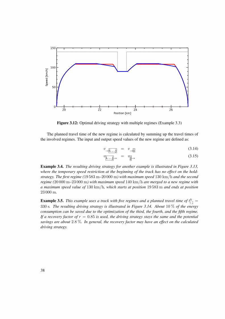
Figure 3.12: Optimal driving strategy with multiple regimes (Example 3.3)
The planned travel time of the new regime is calculated by summing up the travel times ofthe involved regimes. The input and output speed values of the new regime are defined as:
v→ i. . . j = v→ i (3.14)
v i. . . j→ = v j→ (3.15)
Example 3.4. The resulting driving strategy for another example is illustrated in Figure 3.13,where the temporary speed restriction at the beginning of the track has no effect on the hold-strategy. The first regime (19 583 m–20 000 m) with maximum speed 130 km/h and the secondregime (20 000 m–23 000 m) with maximum speed 140 km/h are merged to a new regime witha maximum speed value of 130 km/h, which starts at position 19 583 m and ends at position23 000 m.
Example 3.5. This example uses a track with five regimes and a planned travel time of tk�
=
330 s. The resulting driving strategy is illustrated in Figure 3.14. About 10 % of the energyconsumption can be saved due to the optimization of the third, the fourth, and the fifth regime.If a recovery factor of r = 0.85 is used, the driving strategy stays the same and the potentialsavings are about 2.8 %. In general, the recovery factor may have an effect on the calculateddriving strategy.
38

Figure 3.13: Optimal driving strategy with merged regimes (Example 3.4)
Figure 3.14: Optimal driving strategy with multiple regimes (Example 3.5)
3.4 Algorithm-Parameters
As already mentioned, there are several parameters to configure the algorithm:
• Accuracy vs. computation time: There exist two parameters v+ and s+ which can be usedto configure the accuracy of the results. As a consequence, the computation time dependson these parameters.
39
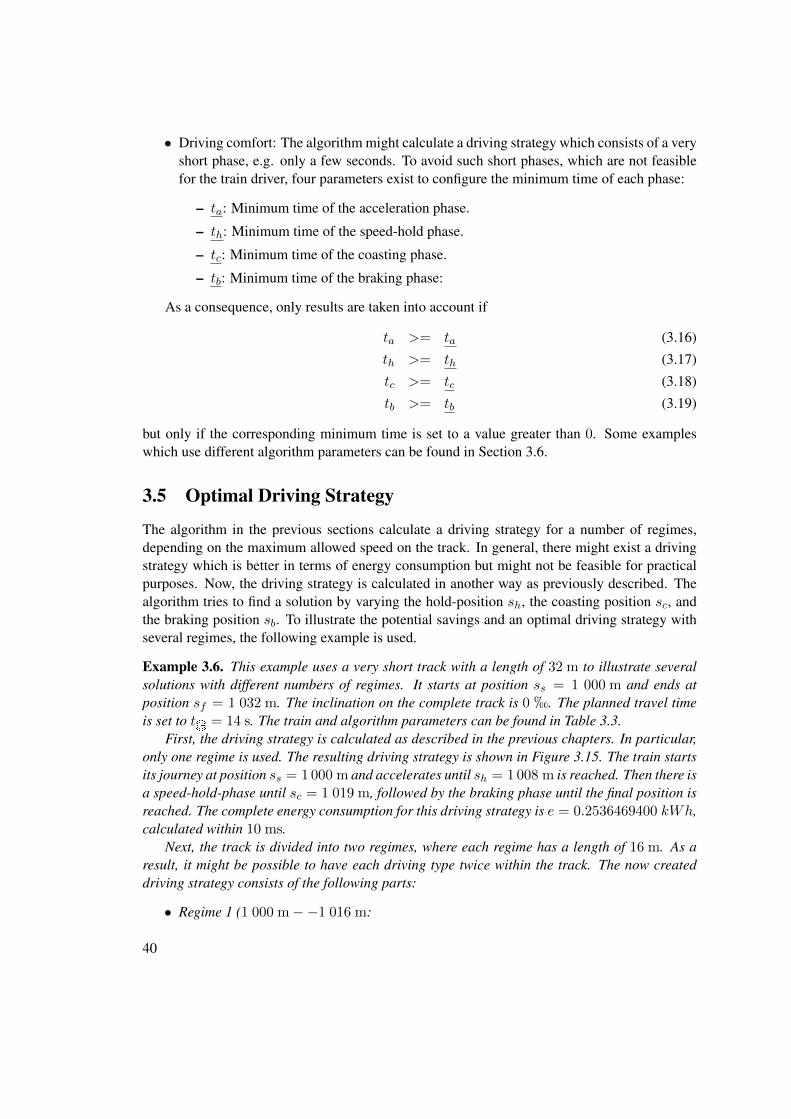
• Driving comfort: The algorithm might calculate a driving strategy which consists of a veryshort phase, e.g. only a few seconds. To avoid such short phases, which are not feasiblefor the train driver, four parameters exist to configure the minimum time of each phase:
– ta: Minimum time of the acceleration phase.
– th: Minimum time of the speed-hold phase.
– tc: Minimum time of the coasting phase.
– tb: Minimum time of the braking phase:
As a consequence, only results are taken into account if
ta >= ta (3.16)
th >= th (3.17)
tc >= tc (3.18)
tb >= tb (3.19)
but only if the corresponding minimum time is set to a value greater than 0. Some exampleswhich use different algorithm parameters can be found in Section 3.6.
3.5 Optimal Driving Strategy
The algorithm in the previous sections calculate a driving strategy for a number of regimes,depending on the maximum allowed speed on the track. In general, there might exist a drivingstrategy which is better in terms of energy consumption but might not be feasible for practicalpurposes. Now, the driving strategy is calculated in another way as previously described. Thealgorithm tries to find a solution by varying the hold-position sh, the coasting position sc, andthe braking position sb. To illustrate the potential savings and an optimal driving strategy withseveral regimes, the following example is used.
Example 3.6. This example uses a very short track with a length of 32 m to illustrate severalsolutions with different numbers of regimes. It starts at position ss = 1 000 m and ends atposition sf = 1 032 m. The inclination on the complete track is 0 h. The planned travel timeis set to t
�= 14 s. The train and algorithm parameters can be found in Table 3.3.
First, the driving strategy is calculated as described in the previous chapters. In particular,only one regime is used. The resulting driving strategy is shown in Figure 3.15. The train startsits journey at position ss = 1 000 m and accelerates until sh = 1 008 m is reached. Then there isa speed-hold-phase until sc = 1 019 m, followed by the braking phase until the final position isreached. The complete energy consumption for this driving strategy is e = 0.2536469400 kWh,calculated within 10 ms.
Next, the track is divided into two regimes, where each regime has a length of 16 m. As aresult, it might be possible to have each driving type twice within the track. The now createddriving strategy consists of the following parts:
• Regime 1 (1 000 m−−1 016 m:
40

Parameter Value Parameter Value
mT 46 000 t mW 74 000 tn 2 r 0.00
F (v) see Ex. 2.1 B(v) see Ex. 2.2l 67 m fL 3.3
kSt1 0.03 kg · s2/m2 kSa1 0.0025 s/mkSa2 0.00696 kg · s2/m2 ∆v 4.17 m/sρ 6 s+ 1 m
Table 3.3: Train and algorithm parameters (Example 3.6)
1.00 1.01 1.02 1.030
5
10
15
20
Position [km]
Spe
ed [k
m/h
]
Figure 3.15: Resulting driving strategy with one regime (Example 3.6)
– Accelerating to 1 007 m.
– Coasting to 1 016 m.
• Regime 2 (1 016 m−−1 032 m:
– Hold the current speed to 1 018 m.
– Coasting to 1 021 m.
– Braking to 1 032 m.
As a consequence, the speed-hold-phase and the coasting phase from the driving strategyin Figure 3.15 is divided into a coasting phase, followed by a speed-hold phase and again a
41
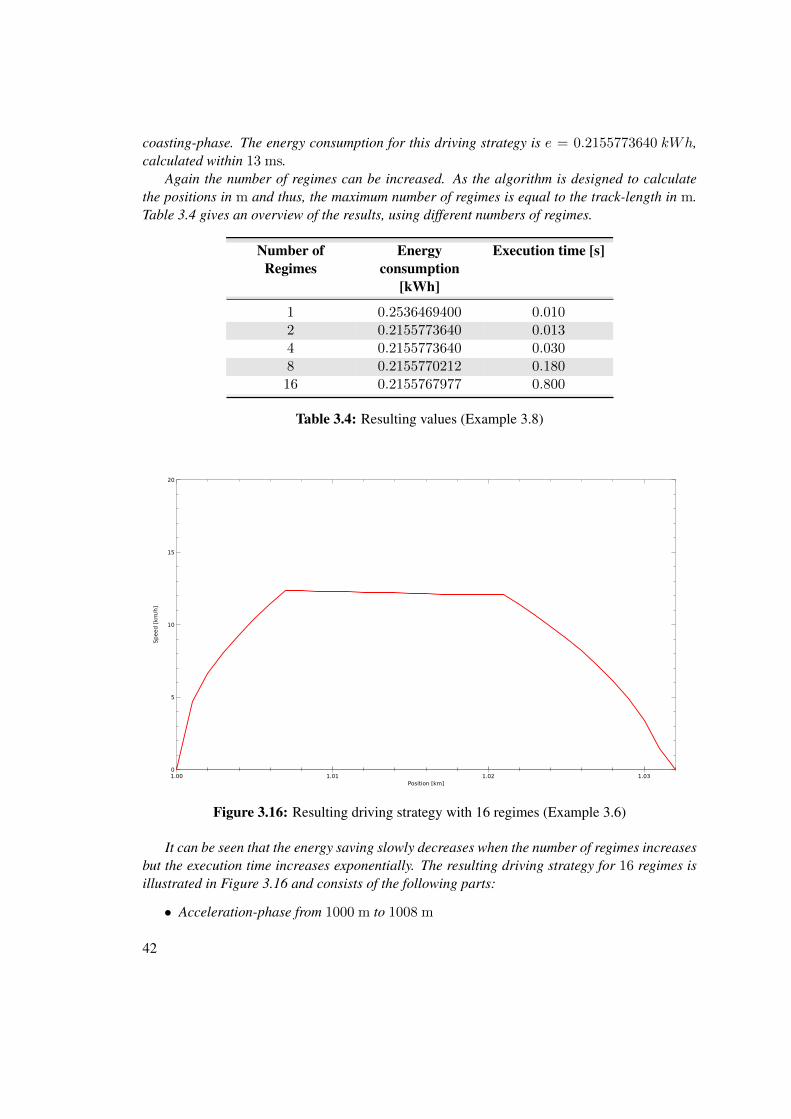
coasting-phase. The energy consumption for this driving strategy is e = 0.2155773640 kWh,calculated within 13 ms.
Again the number of regimes can be increased. As the algorithm is designed to calculatethe positions in m and thus, the maximum number of regimes is equal to the track-length in m.Table 3.4 gives an overview of the results, using different numbers of regimes.
Number ofRegimes
Energyconsumption
[kWh]
Execution time [s]
1 0.2536469400 0.0102 0.2155773640 0.0134 0.2155773640 0.0308 0.2155770212 0.18016 0.2155767977 0.800
Table 3.4: Resulting values (Example 3.8)
1.00 1.01 1.02 1.030
5
10
15
20
Position [km]
Speed [
km/h
]
Figure 3.16: Resulting driving strategy with 16 regimes (Example 3.6)
It can be seen that the energy saving slowly decreases when the number of regimes increasesbut the execution time increases exponentially. The resulting driving strategy for 16 regimes isillustrated in Figure 3.16 and consists of the following parts:
• Acceleration-phase from 1000 m to 1008 m
42

• Coasting-phase from 1008 m to 1019 m
• Speed-hold-phase from 1019 m to 1020 m
• Coasting-phase from 1020 m to 1021 m
• Speed-hold-phase from 1021 m to 1022 m
• Braking-phase from 1022 m to 1032 m
Example 3.7. To illustrate the behavior of the algorithm and the potential of saving trac-tion energy this example will use several changes of the track inclination, given in Table 3.5.The resulting driving strategy for 1 regime and for 16 regimes are illustrated in Figure 3.17and 3.18, respectively. The traction energy can be decreased from 0.1686721295 kWh to0.1487099230 kWh, which conforms a saving of about 11.8 %.
From [m] To [m] Grad. [h] From [m] To [m] Grad. [h]
1 000 1 002 4 1 002 1 004 81 004 1 006 −6 1 006 1 008 71 008 1 010 6 1 010 1 012 −81 012 1 014 10 1 014 1 016 61 016 1 018 0 1 018 1 020 −41 020 1 022 −3 1 022 1 024 31 024 1 026 7 1 026 1 028 −41 028 1 030 2 1 030 032 −5
Table 3.5: Track inclination (Example 3.7)
A driving strategy like that in the previous examples is definitely not feasible in the field dueto the high number of changes of the driving type. In general, for tracks with much inclinationchanges, a driving strategy with several regimes can save more traction energy than on a trackwith constant gradient.
Due to the computation time and the driving and passenger comfort, the algorithm fromthe previous sections will be used further on. The algorithm of this section is given only fortheoretical reasons.
43
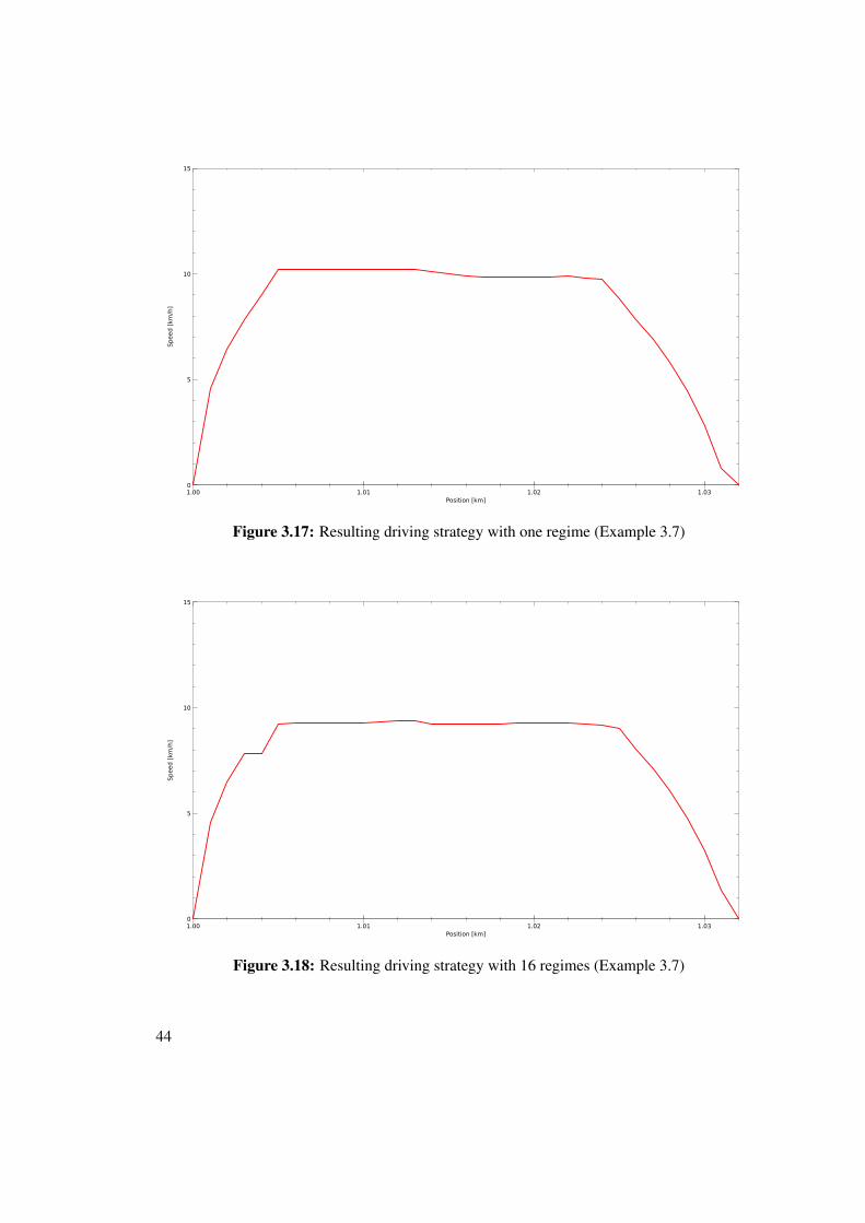
1.00 1.01 1.02 1.030
5
10
15
Position [km]
Speed [
km/h
]
Figure 3.17: Resulting driving strategy with one regime (Example 3.7)
1.00 1.01 1.02 1.030
5
10
15
Position [km]
Speed [
km/h
]
Figure 3.18: Resulting driving strategy with 16 regimes (Example 3.7)
44
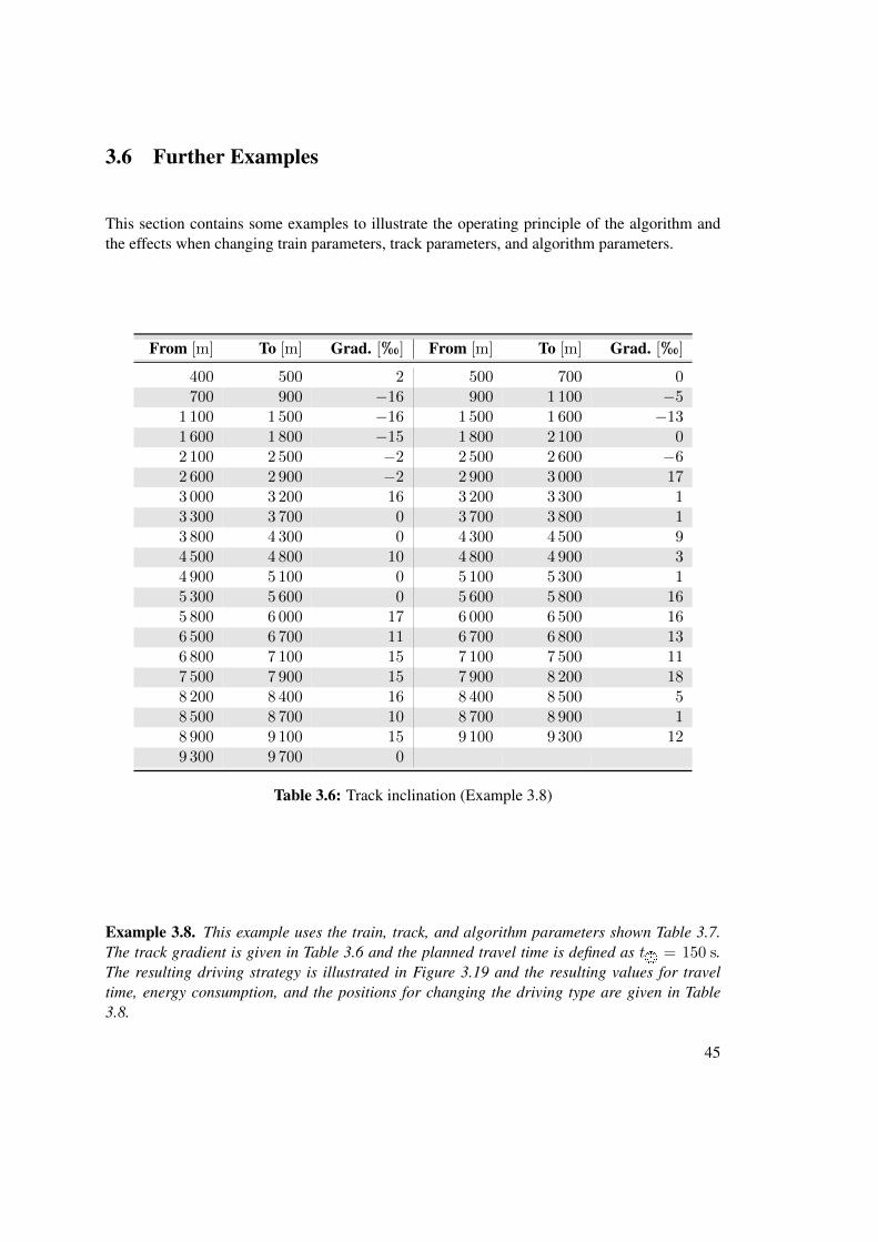
3.6 Further Examples
This section contains some examples to illustrate the operating principle of the algorithm andthe effects when changing train parameters, track parameters, and algorithm parameters.
From [m] To [m] Grad. [h] From [m] To [m] Grad. [h]
400 500 2 500 700 0700 900 −16 900 1 100 −5
1 100 1 500 −16 1 500 1 600 −131 600 1 800 −15 1 800 2 100 02 100 2 500 −2 2 500 2 600 −62 600 2 900 −2 2 900 3 000 173 000 3 200 16 3 200 3 300 13 300 3 700 0 3 700 3 800 13 800 4 300 0 4 300 4 500 94 500 4 800 10 4 800 4 900 34 900 5 100 0 5 100 5 300 15 300 5 600 0 5 600 5 800 165 800 6 000 17 6 000 6 500 166 500 6 700 11 6 700 6 800 136 800 7 100 15 7 100 7 500 117 500 7 900 15 7 900 8 200 188 200 8 400 16 8 400 8 500 58 500 8 700 10 8 700 8 900 18 900 9 100 15 9 100 9 300 129 300 9 700 0
Table 3.6: Track inclination (Example 3.8)
Example 3.8. This example uses the train, track, and algorithm parameters shown Table 3.7.The track gradient is given in Table 3.6 and the planned travel time is defined as t
�= 150 s.
The resulting driving strategy is illustrated in Figure 3.19 and the resulting values for traveltime, energy consumption, and the positions for changing the driving type are given in Table3.8.
45
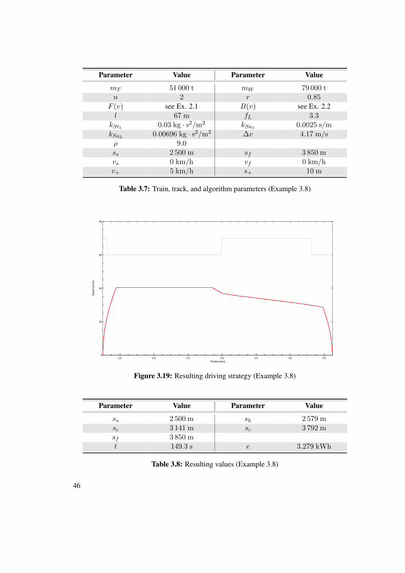
Parameter Value Parameter Value
mT 51 000 t mW 79 000 tn 2 r 0.85
F (v) see Ex. 2.1 B(v) see Ex. 2.2l 67 m fL 3.3
kSt1 0.03 kg · s2/m2 kSa1 0.0025 s/mkSa2 0.00696 kg · s2/m2 ∆v 4.17 m/sρ 9.0ss 2 500 m sf 3 850 mvs 0 km/h vf 0 km/hv+ 5 km/h s+ 10 m
Table 3.7: Train, track, and algorithm parameters (Example 3.8)
2.6 2.8 3.0 3.2 3.4 3.6 3.80
20
40
60
80
Position [km]
Spe
ed [k
m/h
]
Figure 3.19: Resulting driving strategy (Example 3.8)
Parameter Value Parameter Value
ss 2 500 m sh 2 579 msc 3 141 m sc 3 792 msf 3 850 mt 149.3 s e 3.279 kWh
Table 3.8: Resulting values (Example 3.8)
46
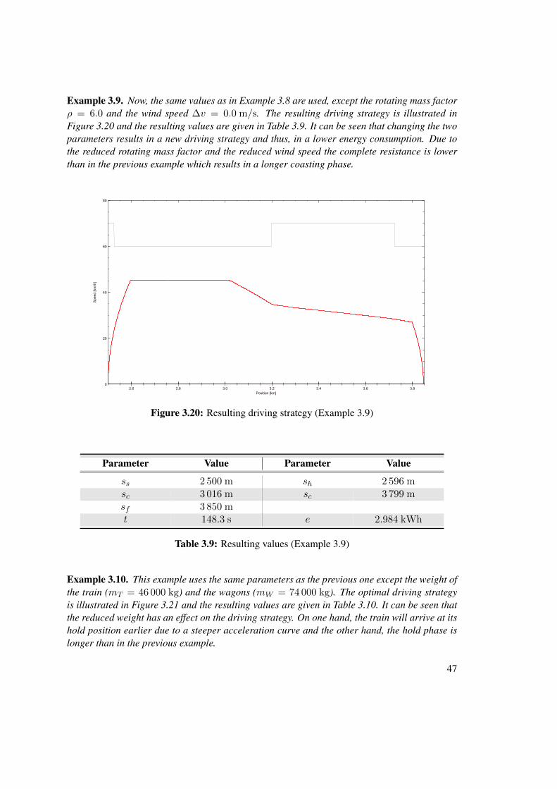
Example 3.9. Now, the same values as in Example 3.8 are used, except the rotating mass factorρ = 6.0 and the wind speed ∆v = 0.0 m/s. The resulting driving strategy is illustrated inFigure 3.20 and the resulting values are given in Table 3.9. It can be seen that changing the twoparameters results in a new driving strategy and thus, in a lower energy consumption. Due tothe reduced rotating mass factor and the reduced wind speed the complete resistance is lowerthan in the previous example which results in a longer coasting phase.
2.6 2.8 3.0 3.2 3.4 3.6 3.80
20
40
60
80
Position [km]
Spe
ed [k
m/h
]
Figure 3.20: Resulting driving strategy (Example 3.9)
Parameter Value Parameter Value
ss 2 500 m sh 2 596 msc 3 016 m sc 3 799 msf 3 850 mt 148.3 s e 2.984 kWh
Table 3.9: Resulting values (Example 3.9)
Example 3.10. This example uses the same parameters as the previous one except the weight ofthe train (mT = 46 000 kg) and the wagons (mW = 74 000 kg). The optimal driving strategyis illustrated in Figure 3.21 and the resulting values are given in Table 3.10. It can be seen thatthe reduced weight has an effect on the driving strategy. On one hand, the train will arrive at itshold position earlier due to a steeper acceleration curve and the other hand, the hold phase islonger than in the previous example.
47
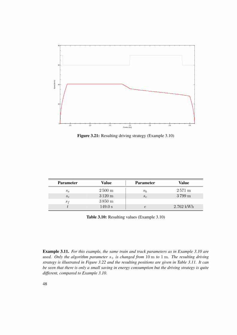
2.6 2.8 3.0 3.2 3.4 3.6 3.80
20
40
60
80
Position [km]
Spe
ed [k
m/h
]
Figure 3.21: Resulting driving strategy (Example 3.10)
Parameter Value Parameter Value
ss 2 500 m sh 2 571 msc 3 120 m sc 3 799 msf 3 850 mt 149.0 s e 2.762 kWh
Table 3.10: Resulting values (Example 3.10)
Example 3.11. For this example, the same train and track parameters as in Example 3.10 areused. Only the algorithm parameter s+ is changed from 10 m to 1 m. The resulting drivingstrategy is illustrated in Figure 3.22 and the resulting positions are given in Table 3.11. It canbe seen that there is only a small saving in energy consumption but the driving strategy is quitedifferent, compared to Example 3.10.
48

2.6 2.8 3.0 3.2 3.4 3.6 3.80
20
40
60
80
Position [km]
Spe
ed [k
m/h
]
Figure 3.22: Resulting driving strategy (Example 3.11)
Parameter Value Parameter Value
ss 2 500 m sh 2 589 msc 3 008 m sc 3 805 msf 3 850 mt 148.6 s e 2.712 kWh
Table 3.11: Resulting values (Example 3.11)
Example 3.12. The next example uses the same parameters as Example 3.10 but now the recov-ery factor is set to r = 0.0. As a result the energy consumption is much higher and the drivingstrategy is quite different (Figure 3.23, Table 3.12).
49

2.6 2.8 3.0 3.2 3.4 3.6 3.80
20
40
60
80
Position [km]
Spe
ed [k
m/h
]
Figure 3.23: Resulting driving strategy (Example 3.12)
Parameter Value Parameter Value
ss 2 500 m sh 2 610 msc 2 898 m sc 3 809 msf 3 850 mt 148.9 s e 3.525 kWh
Table 3.12: Resulting values (Example 3.12)
Example 3.13. This example shows the impact of changing the minimum time of the speed-holdphase to th = 30 s. As a consequence, the speed-hold phase will be longer (th ≈ 33 s) than inthe previous example (th ≈ 20 s) and as a consequence, the energy consumption is increased(Figure 3.24, Table 3.13).
50
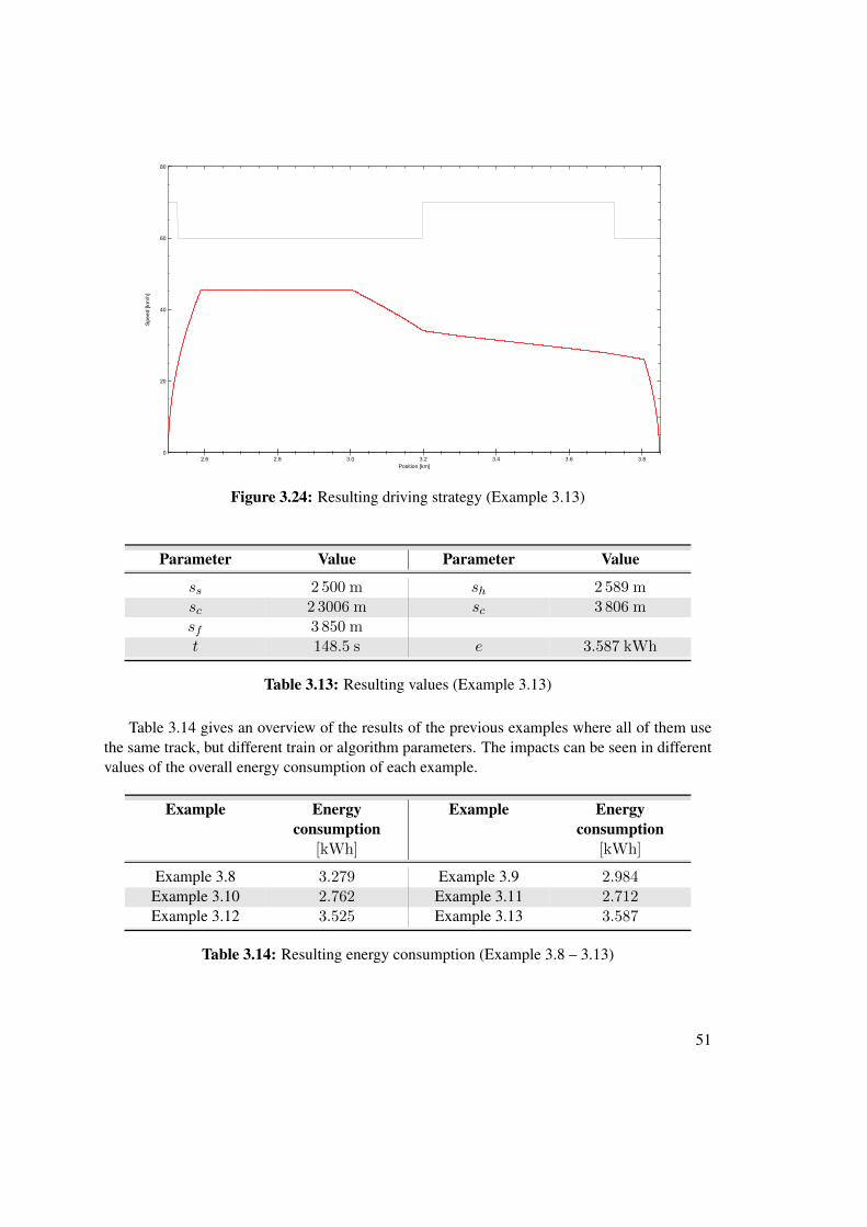
2.6 2.8 3.0 3.2 3.4 3.6 3.80
20
40
60
80
Position [km]
Spe
ed [k
m/h
]
Figure 3.24: Resulting driving strategy (Example 3.13)
Parameter Value Parameter Value
ss 2 500 m sh 2 589 msc 2 3006 m sc 3 806 msf 3 850 mt 148.5 s e 3.587 kWh
Table 3.13: Resulting values (Example 3.13)
Table 3.14 gives an overview of the results of the previous examples where all of them usethe same track, but different train or algorithm parameters. The impacts can be seen in differentvalues of the overall energy consumption of each example.
Example Energyconsumption
[kWh]
Example Energyconsumption
[kWh]
Example 3.8 3.279 Example 3.9 2.984Example 3.10 2.762 Example 3.11 2.712Example 3.12 3.525 Example 3.13 3.587
Table 3.14: Resulting energy consumption (Example 3.8 – 3.13)
51

Example 3.14. This example shows the results of calculating the optimal driving strategy for theÖBB S45 from Wien Breitensee to Wien Heiligenstadt. For the maximum allowed track speedand for the inclination, data from [28] are used. The train characteristics and the algorithmparameters can be found in Table 3.15. The schedule is given in Table 3.16.
Parameter Value Parameter Value
mT 51 000 t mW 79 000 tn 2 r 0.85
F (v) see Ex. 2.1 B(v) see Ex. 2.2l 67 m fL 3.3
kSt1 0.03 kg · s2/m2 kSa1 0.0025 s/mkSa2 0.00696 kg · s2/m2 ∆v 0.00 m/sρ 6.0v+ 5 km/h s+ 1 m
Table 3.15: Train and algorithm parameters (Example 3.14)
Railway station Arrival Departure Travel time
Wien Breitensee 12:05:30Wien Ottakring 12:07:30 12:08:00 00:02:00Wien Hernals 12:10:00 12:10:30 00:02:00Wien Gersthof 12:12:30 12:13:00 00:02:00
Wien Krottenbachstrasse 12:15:30 12:16:00 00:02:30Wien Oberdöbling 12:17:00 12:17:30 00:01:00Wien Heiligenstadt 12:20:30 00:03:00
Table 3.16: Schedule of Example 3.14
The complete journey has an overall energy consumption of e = 1.175 kWh, due to lowdriving speeds and the track inclination. Figure 3.25 shows the resulting driving strategy. Table3.17 gives an overview about the results, consisting of the following columns:
• Driving type (Acceleration phase, speed-Hold phase, Coasting phase, Braking phase)
• Start position [m] of the current driving type.
• Final position [m] of the current driving type.
• Speed [km/h] at the start position of the current driving type.
• Speed [km/h] at the final position of the current driving type.
• Accumulated energy consumption [kWh] at the end of the current driving type.
52
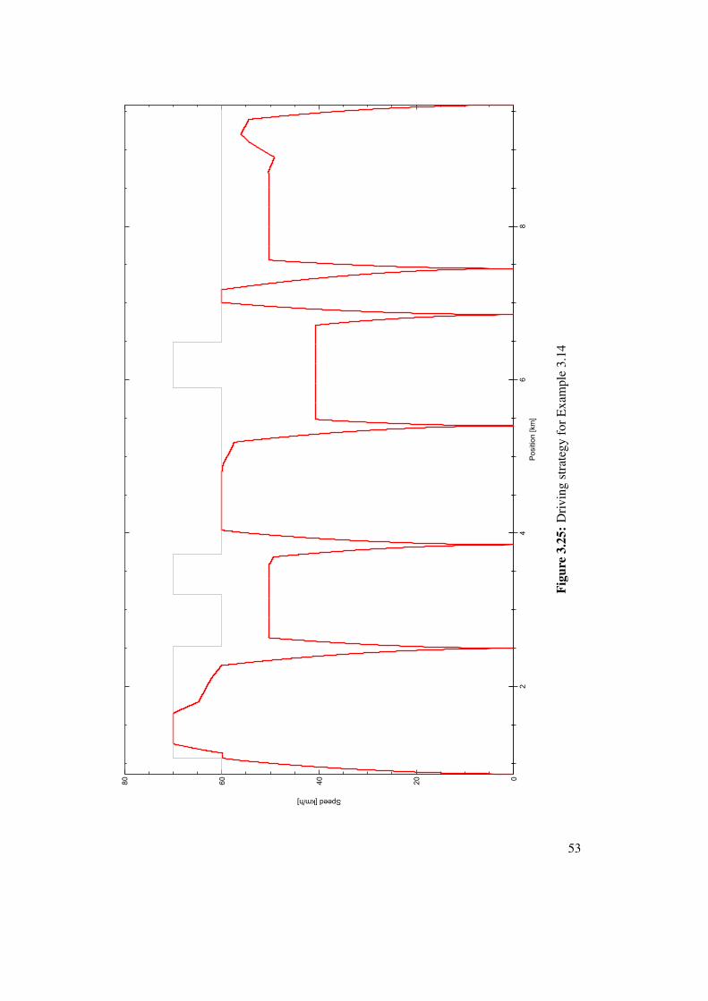
24
68
020406080
Pos
ition
[km
]
Speed [km/h]
Figu
re3.
25:D
rivin
gst
rate
gyfo
rExa
mpl
e3.
14
53
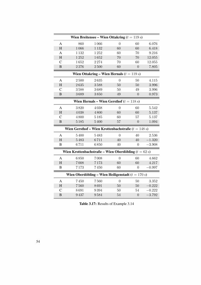
Wien Breitensee – Wien Ottakring (t = 119 s)
A 860 1 066 0 60 6.076H 1 066 1 132 60 60 6.418A 1 132 1 252 60 70 9.216H 1 252 1 652 70 70 12.055C 1 652 2 274 70 60 12.055B 2 276 2 500 60 0 7.805
Wien Ottakring – Wien Hernals (t = 119 s)
A 2 500 2 635 0 50 4.115H 2 635 3 588 50 50 3.996C 3 588 3 689 50 49 3.996B 3 689 3 850 49 0 0.973
Wien Hernals – Wien Gersthof (t = 118 s)
A 3 820 4 038 0 60 5.542H 4 038 4 800 60 60 5.137C 4 800 5 185 60 57 5.137B 5 185 5 400 57 0 1.094
Wien Gersthof – Wien Krottenbachstraße (t = 148 s)
A 5 400 5 483 0 40 2.536H 5 483 6 711 40 40 −1.320B 6 711 6 850 40 0 −3.908
Wien Krottenbachstraße – Wien Oberdöbling (t = 62 s)
A 6 850 7 008 0 60 4.662H 7 008 7 173 60 60 4.217B 7 173 7 450 60 0 −0.997
Wien Oberdöbling – Wien Heiligenstadt (t = 170 s)
A 7 450 7 560 0 50 3.352H 7 560 8 691 50 50 −0.222C 8 691 9 394 50 54 −0.222B 9 437 9 584 54 0 −3.792
Table 3.17: Results of Example 3.14
54

CHAPTER 4Kronecker Algebra
Kronecker Algebra consists of Kronecker Sum and Kronecker Product [56]. This chapter de-scribes the mathematical background, the application of Kronecker Algebra in railway opera-tion, and the representation of routes, track sections, and the behavior of the complete system.
4.1 Introduction to Kronecker Algebra
Kronecker Algebra was introduced to model concurrent systems (cf. [56]), in particular for com-puter systems consisting of several threads which access shared memory. The model was modi-fied for the usage in railway systems (cf. [58, 76–81]). A short overview of several applicationslike travel time analysis or energy awareness are given at the end of this chapter.
Kronecker Sum and Kronecker Product are simple matrix operations, which can be used tomodel synchronization of shared resources and generate interleavings. In the following, bothoperations will be defined. The used matrices will be out of M = {M = (mi,j)|mi,j ∈ L}and only matrices M ∈ M will be used furthermore. Let o(M) refer to the order of matrixM ∈M1. Further on n-by-n zero matrices Zn = (zi,j), where ∀i, j : zi,j = 0 will be used.
In computer science, the access to a shared memory by several threads must be synchronizedand for this reason Kronecker Algebra is applied. In contrast to computer science, trains areused instead of threads and track sections instead of shared memory for railway systems. Theaccess to the resource is modeled by semaphores in the sense of computer science (cf. [19]). Asa result, a train can enter a track section only if it is not occupied by another train.
The application of Kronecker Algebra allows finding conflicts (e.g. headway-conflicts, dead-locks). The resulting graph shows all possible movements of the trains and based on this graph,a conflict-free situation can be found (if it is possible, due to the given timetable). Further details
1A k-by-k matrix is known as square matrix of order k.
55

can be found in the description of the optimization algorithm in Chapter 5. Other approaches tryto find a conflict-free situation by adding the trains successively into the time-distance diagram(cf. [39], Introduction in Chapter 1). That will be possible only for small railway systems with asmall amount of trains.
Representation
As already mentioned, Kronecker Algebra is a mathematical model which can be used to cal-culate a matrix describing a complete railway system. Directed graphs are used to represent themovements of the trains and the operations on track sections. Each train is assigned at least oneroute consisting of at least one track section. A track section can be part of several routes. As aresult the routes describe the movement of the trains and can be represented as graphs, too. Eachgraph can be represented by its adjacency matrix which will be used as input for the calculations.
Assume that the edges in the graphs are labeled by elements of a semiring. Definitions andproperties can be found in [44, 56]. The semiring consists of a set of labels L containing thefollowing semaphore calls (cf. [19]):
• pi denotes entering or reserving track section i, in particular Tj .pi means that train j wantsto enter track section i.
• vi denotes leaving or releasing track section i, in particular Tj .vi means that train j willleave track section i.
A railroad system consists of several trains and track sections which are represented by graphsand their adjacency matrices. In general, binary semaphores are used to represent the operationson track sections, whereas each track section is modeled by its own semaphore. If an operationalstandard allows entry into an occupied block (permissive driving), this approach can deal withthis issue as well by fine-scaling the track section or by using counting semaphores instead ofbinary semaphores. Each edge in the graphs is labeled by l ∈ L. If there exists an edge labeled afrom node i to node j, then the corresponding adjacency matrix M has mi,j = a. If there existsno edge between two nodes, then mi,j = 0.
Definition 4.1 (System model). The system model consists of the tuple 〈T ,S,L〉, where T andS refer to the set of graph adjacency matrices describing the train routes and the track sections,respectively. The labels in T ∈ T and S ∈ S are elements of L.
A directed labeled graphG = 〈V,E, ne〉 consists of a set of labeled nodes V , a set of labeleddirected edges E ⊆ V × V , and an entry node ne. The previously mentioned set V and E areout of 〈T ,S,L〉. A detailed description of the representation can be found in [56].
4.2 Modeling synchronization
Definition 4.2 (Kronecker Product [56]). Given am-by-nmatrixA and a p-by-q matrixB, theirKronecker Product denoted by A⊗B is a mp-by-nq block matrix defined by
56
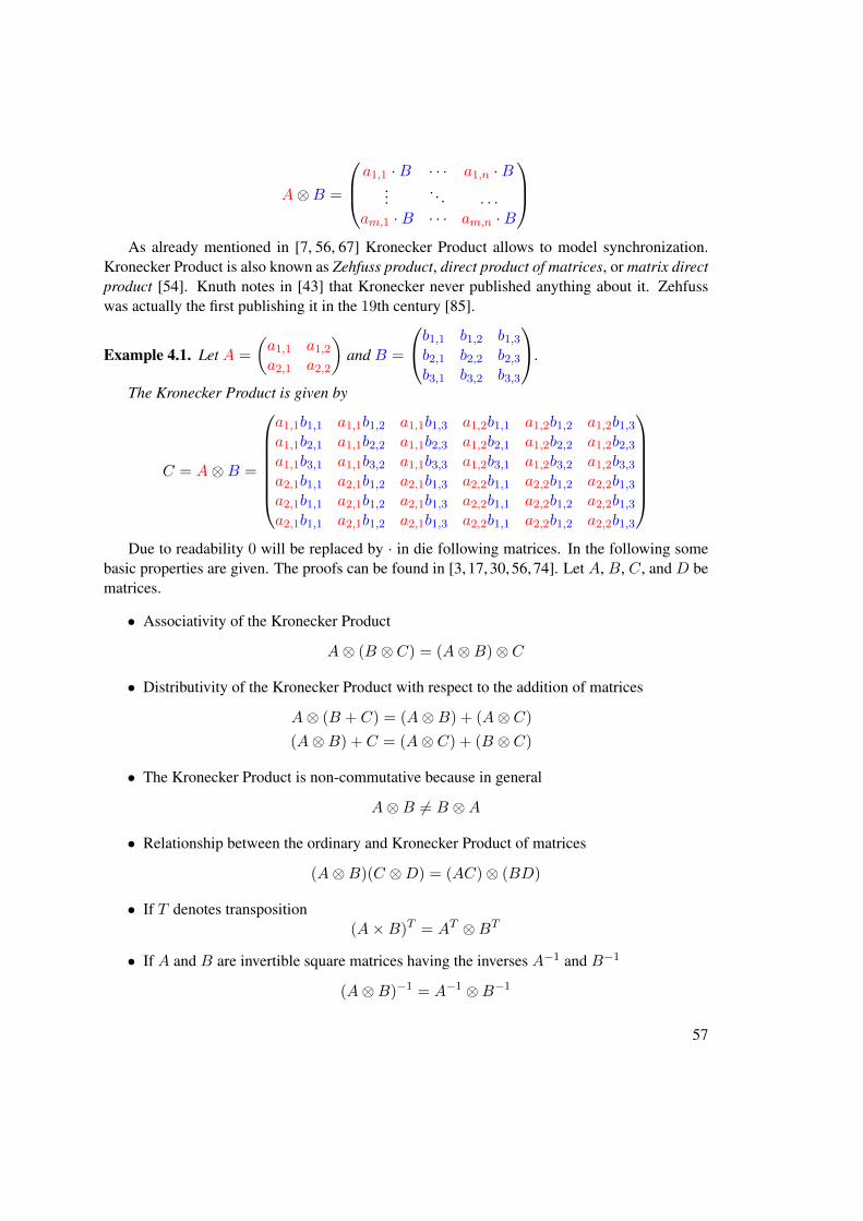
A⊗B =
a1,1 ·B · · · a1,n ·B...
. . . . . .am,1 ·B · · · am,n ·B
As already mentioned in [7, 56, 67] Kronecker Product allows to model synchronization.
Kronecker Product is also known as Zehfuss product, direct product of matrices, or matrix directproduct [54]. Knuth notes in [43] that Kronecker never published anything about it. Zehfusswas actually the first publishing it in the 19th century [85].
Example 4.1. Let A =
(a1,1 a1,2a2,1 a2,2
)and B =
b1,1 b1,2 b1,3b2,1 b2,2 b2,3b3,1 b3,2 b3,3
.
The Kronecker Product is given by
C = A⊗B =
a1,1b1,1 a1,1b1,2 a1,1b1,3 a1,2b1,1 a1,2b1,2 a1,2b1,3a1,1b2,1 a1,1b2,2 a1,1b2,3 a1,2b2,1 a1,2b2,2 a1,2b2,3a1,1b3,1 a1,1b3,2 a1,1b3,3 a1,2b3,1 a1,2b3,2 a1,2b3,3a2,1b1,1 a2,1b1,2 a2,1b1,3 a2,2b1,1 a2,2b1,2 a2,2b1,3a2,1b1,1 a2,1b1,2 a2,1b1,3 a2,2b1,1 a2,2b1,2 a2,2b1,3a2,1b1,1 a2,1b1,2 a2,1b1,3 a2,2b1,1 a2,2b1,2 a2,2b1,3
Due to readability 0 will be replaced by · in die following matrices. In the following some
basic properties are given. The proofs can be found in [3, 17, 30, 56, 74]. Let A, B, C, and D bematrices.
• Associativity of the Kronecker Product
A⊗ (B ⊗ C) = (A⊗B)⊗ C
• Distributivity of the Kronecker Product with respect to the addition of matrices
A⊗ (B + C) = (A⊗B) + (A⊗ C)
(A⊗B) + C = (A⊗ C) + (B ⊗ C)
• The Kronecker Product is non-commutative because in general
A⊗B 6= B ⊗A
• Relationship between the ordinary and Kronecker Product of matrices
(A⊗B)(C ⊗D) = (AC)⊗ (BD)
• If T denotes transposition(A×B)T = AT ⊗BT
• If A and B are invertible square matrices having the inverses A−1 and B−1
(A⊗B)−1 = A−1 ⊗B−1
57

4.3 Generating interleavings
Definition 4.3 (Kronecker Sum [30, 45, 56, 68]). Given a matrix A of order m and a matrix Bof order n, their Kronecker sum denoted by A⊕B is a matrix of order mn defined by
A⊕B = A⊗ In + Im ⊗B (4.1)
where Im and In denote the identity matrices2 of order m and n, respectively.
In general, Kronecker Sum calculates the Cartesian product graph of two graphs adjacencymatrices (cf. [38, 43, 56]).
Example 4.2. Let A =
(a1,1 a1,2a2,1 a2,2
)and B =
b1,1 b1,2 b1,3b2,1 b2,2 b2,3b3,1 b3,2 b3,3
.
The Kronecker Sum is given by
C = A⊕B= A⊗ I3 + I2 ⊗B
=
(a1,1 a1,2a2,1 a2,2
)⊗
1 · ·· 1 ·· · 1
+
(1 ·· 1
)⊗
b1,1 b1,2 b1,3b2,1 b2,2 b2,3b3,1 b3,2 b3,3
=
a1,1 · · a1,2 · ·· a1,1 · · a1,2 ·· · a1,1 · · a1,2a2,1 · · a2,2 · ·· a2,1 · · a2,2 ·· · a2,1 · · a2,2
+
b1,1 b1,2 b1,3 · · ·b2,1 b2,2 b2,3 · · ·b3,1 b3,2 b3,3 · · ·· · · b1,1 b1,2 b1,3· · · b2,1 b2,2 b2,3· · · b3,1 b3,2 b3,3
=
a1,1 + b1,1 b1,2 b1,3 a1,2 · ·b2,1 a1,1 + b2,2 b2,3 · a1,2 ·b3,1 b3,2 a1,1 + b3,3 · · a1,2a2,1 · · a2,2 + b1,1 b1,2 b1,3· a2,1 · b2,1 a2,2 + b2,2 b2,3· · a2,1 b3,1 b3,2 a2,2 + b3,3
In the following some basic properties of Kronecker Sum are given. Their proofs can be
found in [45, 56, 68].
• Let the matrices A and C have order m and B and D have order n. Then
(A⊕B) + (C ⊕D) = (A+ C)⊕ (B +D)
is called Mixed Sum Rule.
2The identity matrix In is a n-by-n square-matrix with ones on the main diagonal and zeros elsewhere
58
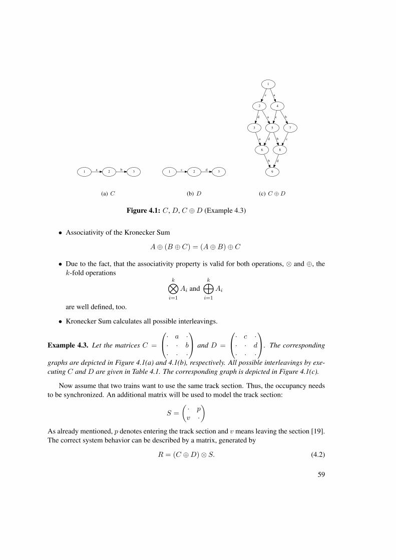
1 2a 3b
(a) C
1 2c 3d
(b) D
1
2
c
4
a
3
d
5
a c
7
b
6
a d
8
b c
9
b d
(c) C ⊕D
Figure 4.1: C, D, C ⊕D (Example 4.3)
• Associativity of the Kronecker Sum
A⊕ (B ⊕ C) = (A⊕B)⊕ C
• Due to the fact, that the associativity property is valid for both operations, ⊗ and ⊕, thek-fold operations
k⊗i=1
Ai andk⊕
i=1
Ai
are well defined, too.
• Kronecker Sum calculates all possible interleavings.
Example 4.3. Let the matrices C =
· a ·· · b· · ·
and D =
· c ·· · d· · ·
. The corresponding
graphs are depicted in Figure 4.1(a) and 4.1(b), respectively. All possible interleavings by exe-cuting C and D are given in Table 4.1. The corresponding graph is depicted in Figure 4.1(c).
Now assume that two trains want to use the same track section. Thus, the occupancy needsto be synchronized. An additional matrix will be used to model the track section:
S =
(· pv ·
)As already mentioned, p denotes entering the track section and v means leaving the section [19].The correct system behavior can be described by a matrix, generated by
R = (C ⊕D)⊗ S. (4.2)
59
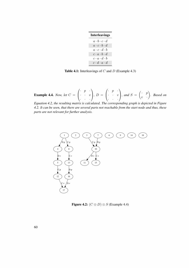
Interleavings
a · b · c · da · c · b · da · c · d · bc · a · b · dc · a · d · bc · d · a · d
Table 4.1: Interleavings of C and D (Example 4.3)
Example 4.4. Now, let C =
· p ·· · v· · ·
, D =
· p ·· · v· · ·
, and S =
(· pv ·
). Based on
Equation 4.2, the resulting matrix is calculated. The corresponding graph is depicted in Figure4.2. It can be seen, that there are several parts not reachable from the start node and thus, theseparts are not relevant for further analysis.
1
4
D.p
8
C.p
5
D.v
12
C.p
17
C.v
13
C.v
16
D.p
D.v
2 3
10
C.p
11
D.v
15
C.v
7
D.p
6 9 14 18
Figure 4.2: (C ⊕D)⊗ S (Example 4.4)
60

4.4 System Model
In general, a railway system consists of a set of trains L = {Lj |1 ≤ j ≤ t}. Each train Lj has arouteRj , which is a sequence of track sections, whereas each track section is modeled by matrix
Ti =
(· pivi ·
). (4.3)
The set of routes is denoted by R = {Rj |1 ≤ j ≤ t}. The complete system can be described by
S =
t⊕j=1
Rj
⊗( r⊕i=1
Ti
). (4.4)
Example 4.5. Assuming the same system as in Example 4.4, but now with the railway specificnotation. It contains two trains, namely L1 and L2. Both trains want to enter track section 1.Thus, the routes will be as follows.
R1 =
· p1 ·· · v1· · ·
R2 =
· p1 ·· · v1· · ·
Track section 1 is modeled by
S1 =
(· p1v1 ·
)Based on Equation 4.4,
⊕tj=1Rj and
⊕ri=1 Ti are calculated:
t⊕j=1
Rj = R1 ⊕R2
= R1 ⊗ I3 + I3 ⊗R2
=
· · · R1.p1 · · · · ·· · · · R1.p1 · · · ·· · · · · R1.p1 · · ·· · · · · · R1.v1 · ·· · · · · · · R1.v1 ·· · · · · · · · R1.v1· · · · · · · · ·· · · · · · · · ·· · · · · · · · ·
61
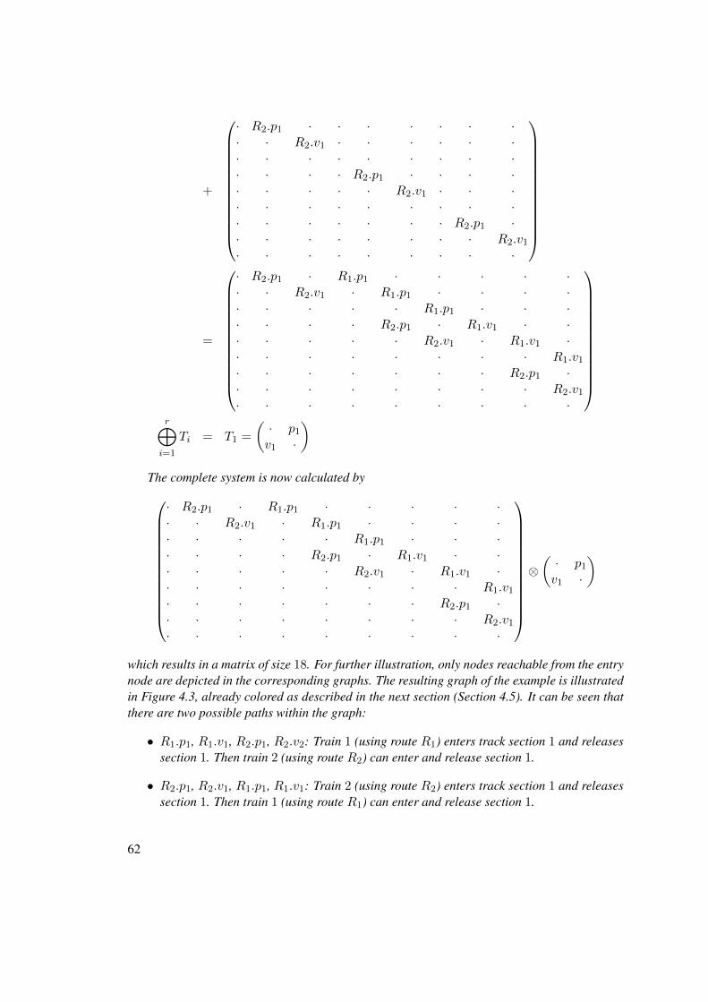
+
· R2.p1 · · · · · · ·· · R2.v1 · · · · · ·· · · · · · · · ·· · · · R2.p1 · · · ·· · · · · R2.v1 · · ·· · · · · · · · ·· · · · · · · R2.p1 ·· · · · · · · · R2.v1· · · · · · · · ·
=
· R2.p1 · R1.p1 · · · · ·· · R2.v1 · R1.p1 · · · ·· · · · · R1.p1 · · ·· · · · R2.p1 · R1.v1 · ·· · · · · R2.v1 · R1.v1 ·· · · · · · · · R1.v1· · · · · · · R2.p1 ·· · · · · · · · R2.v1· · · · · · · · ·
r⊕
i=1
Ti = T1 =
(· p1v1 ·
)The complete system is now calculated by
· R2.p1 · R1.p1 · · · · ·· · R2.v1 · R1.p1 · · · ·· · · · · R1.p1 · · ·· · · · R2.p1 · R1.v1 · ·· · · · · R2.v1 · R1.v1 ·· · · · · · · · R1.v1· · · · · · · R2.p1 ·· · · · · · · · R2.v1· · · · · · · · ·
⊗(· p1v1 ·
)
which results in a matrix of size 18. For further illustration, only nodes reachable from the entrynode are depicted in the corresponding graphs. The resulting graph of the example is illustratedin Figure 4.3, already colored as described in the next section (Section 4.5). It can be seen thatthere are two possible paths within the graph:
• R1.p1, R1.v1, R2.p1, R2.v2: Train 1 (using route R1) enters track section 1 and releasessection 1. Then train 2 (using route R2) can enter and release section 1.
• R2.p1, R2.v1, R1.p1, R1.v1: Train 2 (using route R2) enters track section 1 and releasessection 1. Then train 1 (using route R1) can enter and release section 1.
62
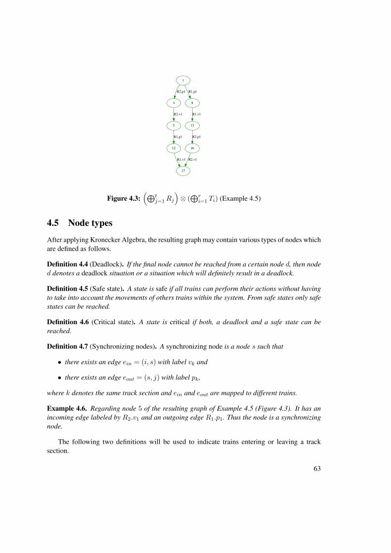
1
4
R2.p1
8
R1.p1
5
R2.v1
13
R1.v1
12
R1.p1
17
R1.v1
16
R2.p1
R2.v1
Figure 4.3:(⊕t
j=1Rj
)⊗ (⊕r
i=1 Ti) (Example 4.5)
4.5 Node types
After applying Kronecker Algebra, the resulting graph may contain various types of nodes whichare defined as follows.
Definition 4.4 (Deadlock). If the final node cannot be reached from a certain node d, then noded denotes a deadlock situation or a situation which will definitely result in a deadlock.
Definition 4.5 (Safe state). A state is safe if all trains can perform their actions without havingto take into account the movements of others trains within the system. From safe states only safestates can be reached.
Definition 4.6 (Critical state). A state is critical if both, a deadlock and a safe state can bereached.
Definition 4.7 (Synchronizing nodes). A synchronizing node is a node s such that
• there exists an edge ein = (i, s) with label vk and
• there exists an edge eout = (s, j) with label pk,
where k denotes the same track section and ein and eout are mapped to different trains.
Example 4.6. Regarding node 5 of the resulting graph of Example 4.5 (Figure 4.3). It has anincoming edge labeled by R2.v1 and an outgoing edge R1.p1. Thus the node is a synchronizingnode.
The following two definitions will be used to indicate trains entering or leaving a tracksection.
63
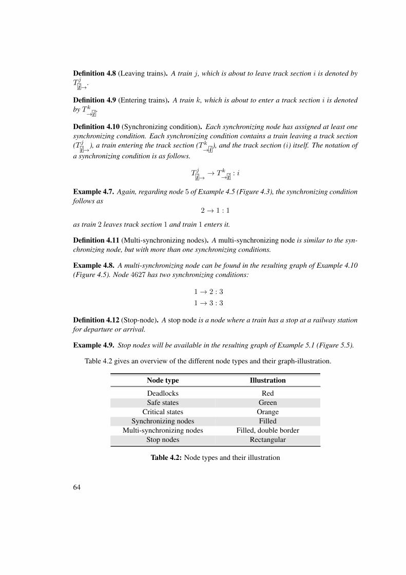
Definition 4.8 (Leaving trains). A train j, which is about to leave track section i is denoted byT j
i→.
Definition 4.9 (Entering trains). A train k, which is about to enter a track section i is denotedby T k
→ i .
Definition 4.10 (Synchronizing condition). Each synchronizing node has assigned at least onesynchronizing condition. Each synchronizing condition contains a train leaving a track section(T j
i→), a train entering the track section (T k→ i ), and the track section (i) itself. The notation of
a synchronizing condition is as follows.
T j
i→ → T k→ i : i
Example 4.7. Again, regarding node 5 of Example 4.5 (Figure 4.3), the synchronizing conditionfollows as
2→ 1 : 1
as train 2 leaves track section 1 and train 1 enters it.
Definition 4.11 (Multi-synchronizing nodes). A multi-synchronizing node is similar to the syn-chronizing node, but with more than one synchronizing conditions.
Example 4.8. A multi-synchronizing node can be found in the resulting graph of Example 4.10(Figure 4.5). Node 4627 has two synchronizing conditions:
1→ 2 : 3
1→ 3 : 3
Definition 4.12 (Stop-node). A stop node is a node where a train has a stop at a railway stationfor departure or arrival.
Example 4.9. Stop nodes will be available in the resulting graph of Example 5.1 (Figure 5.5).
Table 4.2 gives an overview of the different node types and their graph-illustration.
Node type Illustration
Deadlocks RedSafe states Green
Critical states OrangeSynchronizing nodes Filled
Multi-synchronizing nodes Filled, double borderStop nodes Rectangular
Table 4.2: Node types and their illustration
64
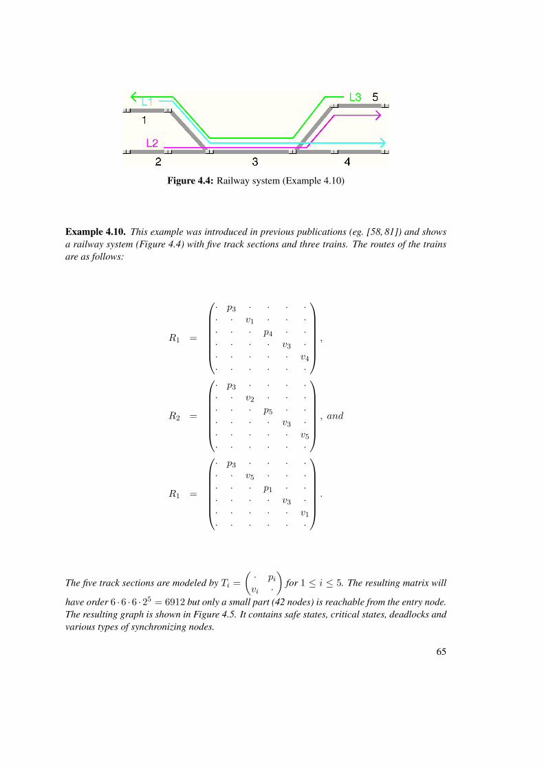
Figure 4.4: Railway system (Example 4.10)
Example 4.10. This example was introduced in previous publications (eg. [58, 81]) and showsa railway system (Figure 4.4) with five track sections and three trains. The routes of the trainsare as follows:
R1 =
· p3 · · · ·· · v1 · · ·· · · p4 · ·· · · · v3 ·· · · · · v4· · · · · ·
,
R2 =
· p3 · · · ·· · v2 · · ·· · · p5 · ·· · · · v3 ·· · · · · v5· · · · · ·
, and
R1 =
· p3 · · · ·· · v5 · · ·· · · p1 · ·· · · · v3 ·· · · · · v1· · · · · ·
.
The five track sections are modeled by Ti =
(· pivi ·
)for 1 ≤ i ≤ 5. The resulting matrix will
have order 6 ·6 ·6 ·25 = 6912 but only a small part (42 nodes) is reachable from the entry node.The resulting graph is shown in Figure 4.5. It contains safe states, critical states, deadlocks andvarious types of synchronizing nodes.
65

1
37
Z3.p3
197
Z2.p3
1157
Z1.p3
70
Z3.v5
397
Z2.v2
2325
Z1.v1
3479
Z1.p4
4627
Z1.v3
5777
Z1.v4
4823
Z2.p3
4663
Z3.p3
5973
Z2.p3
5813
Z3.p3Z1.v4
5023
Z2.v2 Z1.v4
4696
Z3.v5
6173
Z2.v2Z1.v4
5846
Z3.v5
5862
Z3.p1
5890
Z3.v3
5938
Z3.v1
6086
Z2.p3
6134
Z2.p3Z3.v1
6286
Z2.v2
6334
Z2.v2
6525
Z2.p5
6713
Z2.v3
6906
Z2.v5
Z3.v1
6477
Z2.p5
Z3.v1
6665
Z2.v3
Z3.v1
6858
Z2.v5
Z3.v1
Z1.v4
4712
Z3.p1
Z1.v4
4740
Z3.v3
Z1.v4
4936
Z2.p3
4788
Z3.v1
Z1.v4
4984
Z3.v1
5136
Z2.v2 Z1.v4Z2.p3
Z1.v4
5184
Z2.v2Z1.v4Z3.v1
5327
Z2.p5
Z1.v4
5375
Z2.p5
Z1.v4
5563
Z2.v3
Z1.v4
5756
Z2.v5
Z1.v4Z3.v1
5515
Z2.v3
Z1.v4Z3.v1
5708
Z2.v5
Z1.v4Z3.v1
Z1.v4
Figure 4.5: Resulting graph (Example 4.10)
66
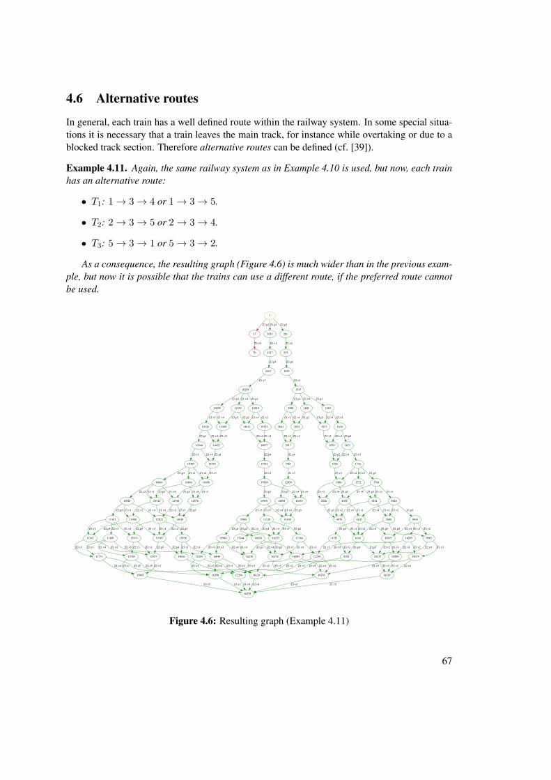
4.6 Alternative routes
In general, each train has a well defined route within the railway system. In some special situa-tions it is necessary that a train leaves the main track, for instance while overtaking or due to ablocked track section. Therefore alternative routes can be defined (cf. [39]).
Example 4.11. Again, the same railway system as in Example 4.10 is used, but now, each trainhas an alternative route:
• T1: 1→ 3→ 4 or 1→ 3→ 5.
• T2: 2→ 3→ 5 or 2→ 3→ 4.
• T3: 5→ 3→ 1 or 5→ 3→ 2.
As a consequence, the resulting graph (Figure 4.6) is much wider than in the previous exam-ple, but now it is possible that the trains can use a different route, if the preferred route cannotbe used.
1
37
Z3.p3
2053
Z1.p3
261
Z2.p3
70
Z3.v5
4117
Z1.v1
525
Z2.v2
6167
Z1.p4
10259
Z1.v3
10295
Z3.p3
10519
Z2.p3
14353
Z1.v4
14389
Z1.v4
10328
Z3.v5
10783
Z2.v2
14613
Z1.v4Z3.p3 Z2.p3
14422
Z3.v5Z1.v4
10344
Z3.p1
14877
Z1.v4Z2.v2
15391
Z2.p4
14438
Z3.p1
14498
Z3.v3
14578
Z3.v1
14758
Z2.p3
14838
Z2.p3Z3.v1
15022
Z2.v2
15102
Z2.v2
15536
Z2.p4
15277
Z2.p5 Z3.v1
15616
Z3.v1
16044
Z2.v3
15357
Z3.v1
15785
Z2.v3 Z2.p4Z2.p5
16124
Z2.v3 Z3.v1
16298
Z2.v4
15865
Z2.v3Z2.v5Z3.v1
16378
Z2.v4
15899
Z2.v3
16153
Z2.v4
15935
Z3.p3
Z3.v1Z2.v5
Z1.v4
10404
Z3.v3
Z1.v4
10664
Z2.p3
10484
Z3.v1
Z1.v4
10928
Z2.v2
10744
Z3.v1 Z1.v4Z2.p3
Z1.v4
11183
Z2.p5
11008
Z3.v1 Z1.v4Z2.v2
Z1.v4
11263
Z3.v1
11691
Z2.v3 Z1.v4Z2.p5
Z1.v4
11771
Z2.v3 Z1.v4Z3.v1
12204
Z2.v5
Z1.v4
12284
Z2.v5
Z1.v4
Z1.v4 Z3.v1
1039
Z2.p4
1547
Z2.v3
1583
Z3.p3
3599
Z1.p3
1801
Z2.v4
1616
Z3.v5
1837
Z2.v4
3853
Z2.v4
5663
Z1.v1 Z3.p3Z1.p3
1870
Z2.v4
1672
Z3.p2Z3.v5
1926
Z3.p2 Z2.v4
1732
Z3.v3
1986
Z3.v3
4038
Z1.p3
2026
Z3.v2
6102
Z1.v1
4078
Z3.v2Z1.p3
10197
Z1.p5
8152
Z1.p4
6142
Z3.v2Z1.v1
10237
Z3.v2
14289
Z1.v3
12244
Z1.v3
8192
Z3.v2 Z1.p5Z1.p4
14329
Z1.v3 Z3.v2
16338
Z1.v5
Z1.v5
Z2.v4
3784
Z1.p3
1772
Z3.v2
Z3.v2
Z2.v4
3824
Z3.v2
5848
Z1.v1Z2.v4 Z1.p3
Z2.v4
5888
Z1.v1Z2.v4 Z3.v2
9943
Z1.p5
Z2.v4
9983
Z1.p5
Z2.v4
14075
Z1.v3
Z2.v4 Z3.v2
14035
Z1.v3
Z1.v5 Z2.v4
Z2.v4 Z3.v2
16084
Z1.v5
Z3.v2 Z1.v4Z1.v3Z3.v2 Z2.v4
5917
Z1.v1Z2.v4
7967
Z1.p4
12059
Z1.v3
12095
Z3.p3 Z1.v4
16189
Z1.v4
12128
Z3.v5 Z3.p3
16222
Z3.v5Z1.v4
12144
Z3.p1
12184
Z3.p2
16278
Z3.p2
16238
Z3.p1
Z3.v3Z3.v3
Z3.v3 Z1.v4 Z3.v3Z1.v4
Z2.v4
15968
Z3.v5
Z2.v4
16024
Z3.p2
15984
Z3.p1
Z3.v3Z2.v4Z3.v3 Z2.v4
Figure 4.6: Resulting graph (Example 4.11)
67

4.7 Properties of the resulting matrix
As already proved in [56], the number of edges after the application of Kronecker Sum isO(mn)3. Thus, the number of edges is linear in the order of the resulting adjacency matrix.The number of nodes is bounded from above by nk, where k is the number of trains within therailway system and the route of each train consists of n nodes. Based on Lemma 7 of [56], theresulting matrix, describing the complete railway system, is sparse. This enables the applicationof memory saving data structures and efficient algorithms (e.g. by using adjacency lists, whichare linear in the number of nodes). In the worst case, however, the number of nodes increasesexponentially in the number of trains [56].
Further information about the efficient implementation of the matrix operations and the lazyimplementation of Kronecker Algebra are given in [56] and are not further explained here.
4.8 Lazy Implementation of Kronecker Algebra
The resulting graph after applying Kronecker Algebra contains unreachable parts due to syn-chronization (cf. [56]). For railway systems with lots of synchronizations, the reachable partsmay be very small. This observations motivates the lazy implementation (cf. [31]) describedin [56].
Choosing a lazy implementation for the matrix operations ensures that, when extracting thereachable parts of the underlying graph, the overall effort is reduced to exactly these parts. Bystarting from the graph’s start node and calculating all reachable successors the lazy implemen-tation exactly does this. Thus, for example, if the resulting graph’s size is linear in terms of theinvolved trains, only linear effort will be necessary to generate the graph. Further informationof the implementation can be found in [56].
4.9 Extensions of the model
Travel time analysis
As introduced in [81] the model can be extended to calculate the travel time for each train withinthe railway system. This is based on [57], which is concerned with the Timing Analysis ofConcurrent Programs.
For the travel time analysis each node is assigned a variable and an equation is setup based onthe predecessor. The variable contains a vector where each component of the vector correspondsto a train. The equations are used to calculate the travel time. Additionally, each edge is assigneda travel time value which is used in the equations to calculate the complete travel time for eachtrain. Definitions and examples can be found in [57, 76–78, 80, 81].
3Assuming the corresponding matrices have order m and n, respectively
68

Energy awareness
The model can be extended to use shared resources which can be used by more than one trainsimultaneously. Counting semaphores [19] can be used to model discrete power resources. Inparticular, the available energy is quantized into standardized packages, e.g. 1 MWh. A powerstation or substation produces an amount of energy packages. Trains can reserve a well definedamount of these packages when entering a track section. After leaving a track section, thepackages are released and thus, available for other trains. This model was introduced in [76]and can be used to find deadlocks and to minimize energy demand. Examples can be foundin [76, 77, 79, 80].
Extra-long trains
In the previous examples it was assumed that the length of a train is less than the length ofa track section and thus, the train reserves only two track sections simultaneously. For extra-long trains which are much longer than a track section, several track sections must be reservedsimultaneously. An example for handling such trains can be found in [79] and [76].
69

CHAPTER 5System optimization
Chapter 3 describes the optimization of the driving strategy of a single train. If there are moretrains within a railway network, each train might influence other trains. For instance, a trainwants to enter a track section, which is occupied by another train. In this case, the train has towait until the track section is released.
This chapter describes the optimization of the complete railway system, based on KroneckerAlgebra (Chapter 4) and the single trip optimization (Chapter 3). The algorithm to get the opti-mized behavior in term of energy consumption of all trains within a railway system is explainedin the following sections and consists of several parts:
• Kronecker Algebra based system analysis
• Graph reduction
• Determine all possible routes
• Finding the optimal driving strategy
The explanation of the algorithm will be supported by the following example.
Example 5.1. The railway system is illustrated in Figure 5.1. Each track of the railway systemis divided into track sections and each section has a unique number 1. The example in Figure5.1 consists of seven track sections. The unique number, the start position, and the end positionof each track section are given in Table 5.1.
1The red numbers in Figure 5.1 denote the unique number of the track section. The borders of each track sectionare marked by blue lines.
71

Figure 5.1: Railway System
TrackSection
Start Position[m]
End Position[m]
1 1 000 5 0002 5 000 9 0003 9 000 14 0004 9 000 14 0005 9 000 12 0006 12 000 14 0007 14 000 18 000
Table 5.1: Track sections of railway system (Figure 5.1)
There are three trains within the railway system with the following routes2:
• Train 1 (T1): 1 → 2 → 5 → 6 → 7. Train T1 starts at position 1 000 m at track section1, has a stop at position 12 000 m at the end of section 5 and will finish its journey atposition 18 000 m at track section 7.
• Train 2 (T2): 1→ 2→ 3→ 7. Train T2 starts at position 1 000 m at track section 1 andfinishes its journey at position 18 000 m at section 7 without any further stop.
• Train 3 (T3): 7→ 4→ 2→ 1. The third train (T3) starts its journey at position 18 000 m(section 7) and stops at position 1 000 m at track section 1.
Obviously, the three trains have to use some common track sections (1, 2, and 7). For therailway application it has to be ensured that a track section is occupied by one train only andthus the allocation of the track sections must be analyzed and their access synchronized, toguarantee that there is no overlapping of their blocking-time. This approach will be explainedin the following subsections.
2A route of a train consists of several track sections. A track section can be part of several routes.
72
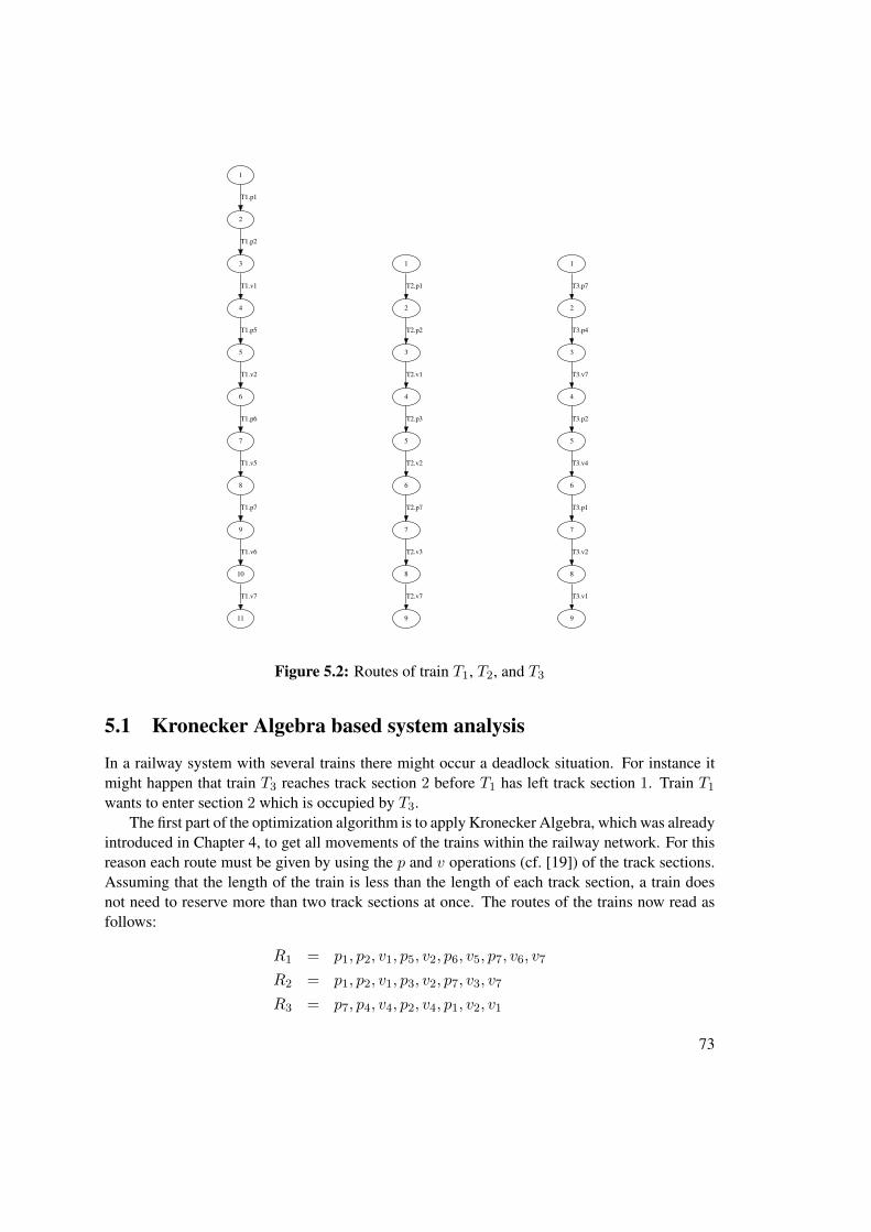
1
2
T1.p1
3
T1.p2
4
T1.v1
5
T1.p5
6
T1.v2
7
T1.p6
8
T1.v5
9
T1.p7
10
T1.v6
11
T1.v7
1
2
T2.p1
3
T2.p2
4
T2.v1
5
T2.p3
6
T2.v2
7
T2.p7
8
T2.v3
9
T2.v7
1
2
T3.p7
3
T3.p4
4
T3.v7
5
T3.p2
6
T3.v4
7
T3.p1
8
T3.v2
9
T3.v1
Figure 5.2: Routes of train T1, T2, and T3
5.1 Kronecker Algebra based system analysis
In a railway system with several trains there might occur a deadlock situation. For instance itmight happen that train T3 reaches track section 2 before T1 has left track section 1. Train T1wants to enter section 2 which is occupied by T3.
The first part of the optimization algorithm is to apply Kronecker Algebra, which was alreadyintroduced in Chapter 4, to get all movements of the trains within the railway network. For thisreason each route must be given by using the p and v operations (cf. [19]) of the track sections.Assuming that the length of the train is less than the length of each track section, a train doesnot need to reserve more than two track sections at once. The routes of the trains now read asfollows:
R1 = p1, p2, v1, p5, v2, p6, v5, p7, v6, v7
R2 = p1, p2, v1, p3, v2, p7, v3, v7
R3 = p7, p4, v4, p2, v4, p1, v2, v1
73
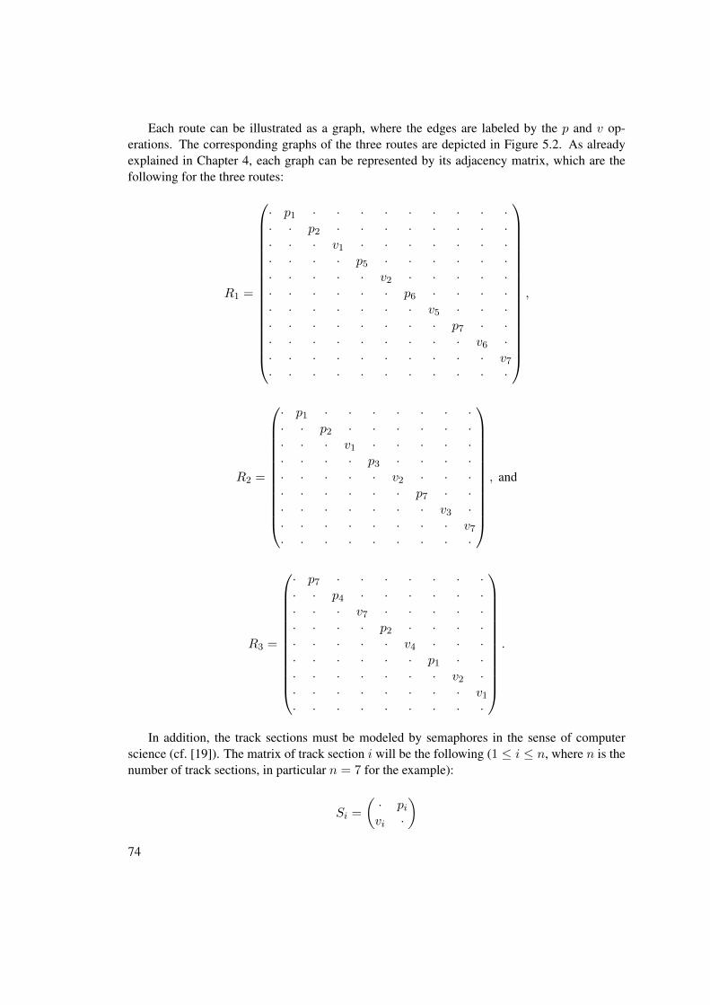
Each route can be illustrated as a graph, where the edges are labeled by the p and v op-erations. The corresponding graphs of the three routes are depicted in Figure 5.2. As alreadyexplained in Chapter 4, each graph can be represented by its adjacency matrix, which are thefollowing for the three routes:
R1 =
· p1 · · · · · · · · ·· · p2 · · · · · · · ·· · · v1 · · · · · · ·· · · · p5 · · · · · ·· · · · · v2 · · · · ·· · · · · · p6 · · · ·· · · · · · · v5 · · ·· · · · · · · · p7 · ·· · · · · · · · · v6 ·· · · · · · · · · · v7· · · · · · · · · · ·
,
R2 =
· p1 · · · · · · ·· · p2 · · · · · ·· · · v1 · · · · ·· · · · p3 · · · ·· · · · · v2 · · ·· · · · · · p7 · ·· · · · · · · v3 ·· · · · · · · · v7· · · · · · · · ·
, and
R3 =
· p7 · · · · · · ·· · p4 · · · · · ·· · · v7 · · · · ·· · · · p2 · · · ·· · · · · v4 · · ·· · · · · · p1 · ·· · · · · · · v2 ·· · · · · · · · v1· · · · · · · · ·
.
In addition, the track sections must be modeled by semaphores in the sense of computerscience (cf. [19]). The matrix of track section i will be the following (1 ≤ i ≤ n, where n is thenumber of track sections, in particular n = 7 for the example):
Si =
(· pivi ·
)74

By applying Kronecker Algebra, a matrix of size 19 200 is created and thus there exist 19 200states. The resulting matrix consists of all possible train movements, including deadlocks. It willbe reduced to the relevant nodes in the following section.
5.2 Graph reduction
The resulting graph after the application of Kronecker Algebra can be reduced to the relevantsynchronizing nodes. The algorithm is designed to run on multi-core CPUs. There are severalrunning tasks, where each task has a unique id, which is a positive integer. The maximumnumber of tasks can be adjusted in the algorithm settings. The graph reduction consists of thefollowing four steps, which are described afterwards:
1. Determine the graph nodes.
2. Find the synchronizing nodes.
3. Check the synchronizing nodes.
4. Find a path between the synchronizing nodes.
Each part is designed to run on multi-core CPUs. Most of the operations are done solelywithin the task. If access to shared memory is unavoidable, it is guarded by protected objects(cf. [5, 75]), which are part of the Ada programming language. After the execution of the tasks,relevant data is copied from the local memory of the tasks to the global program memory.
Part I: Determine the graph nodes
As already mentioned the resulting graph is represented by a matrix. The first step of the graphreduction is to find all nodes, which are reachable from the entry node3. This is done by abreadth-first search, where each reachable node is added to a task-local set of nodes. Afterall nodes are examined, each task copies its data to a global set of nodes. As a result, a graphconsisting of nodes reachable from the entry node remains. In this resulting graph, there might beall types of nodes available, including deadlocks which will be eliminated in the next step. Theremight exist nodes within the resulting graph which are not reachable from the entry node. Thesenodes do not show up because of this reduction procedure. As a consequence, all remainingnodes represent possible states in the railway system and all edges represent train movements,respectively.
The resulting matrix after the application of Kronecker Algebra for the example has size19 200 and thus 19 200 possible states. Due to the reduction the resulting graph is scaled downto 499 nodes which is illustrated in Figure 5.3. It contains red nodes (deadlocks), green nodes(save states), and orange nodes. The entry node has node id 1 and the final node 113 921.
3A node uj is reachable from ui, if there exists a path from ui to uj
75

1 130T3
.p7
1043
3
T1.p
1
1217
T2.p
1
266T3
.p4
1056
2
T1.p
1
1346
T2.p
1T3
.p7
2083
3
T1.p
2T3
.p7
2401T2
.p2
393T3
.v7
1069
8
T1.p
1
1482
T2.p
1T3
.p4
2096
2
T1.p
2T3
.p4
2530
T2.p
2
1082
5
T1.p
1
1609
T2.p
1
553T3
.p2
T3.v
7
2109
8
T1.p
2T3
.v7
2666
T2.p
2T3
.p4 31
266T1
.v1
3618T2
.v1
T3.p
4
1098
5
T3.p
2
2122
5
T1.p
2
1769
T3.p
2
2793
T2.p
2T1
.p1
T2.p
1
673T3
.v4
1110
5
T3.v
4
3152
9
T1.v
1
1889
T3.v
4
3881
T2.v
1T1
.p1
T2.p
1
865T3
.p1
4190
1T1.p
5
3274
5
T2.p
1
T3.v
7 3140
2
T1.v
1T3
.p4
4163
8
T1.p
5
3248
2T2.p
1
T3.v
7
4177
4
T1.p
5
3261
8
T2.p
1
4299
0T2.p
1
5211
0
T1.v
2T3
.v7
T1.p
5T3
.v7
5332
6
T1.v
2
4311
7
T3.v
7T2
.p1
5223
7
T3.v
7
6248
0
T1.p
6T2
.p1
T1.v
2
5451
0
T2.p
2
5345
3
T3.v
7 6369
6
T1.p
6T1
.v2
5559
8
T2.v
1
6488
0
T1.p
6
5463
7
T3.v
7T2
.p2
6382
3
T1.p
6
5361
3
T3.p
2T2
.p2
T3.v
7
7406
0
T1.v
5
T2.p
1
6260
7
T1.p
6
5239
7
T3.p
2T2
.p1
T3.v
7
7284
4
T1.v
5
T1.p
5
5676
6
T2.p
3
5572
5
T3.v
7
6596
8
T1.p
6T2
.v1
6500
7
T3.v
7
7524
4
T1.v
5T2
.v1
T1.p
6
5788
6
T2.v
2
5689
3
T3.v
7
6713
6
T1.p
6T2
.p3
6609
5
T1.p
6T2
.p3
T3.v
7
7633
2
T1.v
5
5801
3T3.v
7
6825
6
T1.p
6T2
.v2
6726
3
T1.p
6T2
.v2
T3.v
7
7750
0
T1.v
5
T2.v
1
7537
1
T1.v
5T3
.v7
T2.v
1
6838
3
T1.p
6
5916
6
T2.p
7
5817
3
T3.p
2T3
.v7
7862
0
T1.v
5
T2.p
3
7645
9
T1.v
5
T2.v
2
7762
7
T1.v
5T2
.p3
8682
8
T1.p
7
6953
6
T2.p
7
6854
3
T3.p
2
7874
7
T1.v
5T2
.v2
8799
6
T1.p
7
6969
6
T3.p
2
7067
2
T2.v
3
7990
0
T1.v
5T2
.p7
6866
3
T3.v
4
7890
7
T1.v
5T2
.p7
T3.p
2
8911
6
T1.p
7
6981
6
T3.v
4
7083
2T2.v
3
8006
0
T1.v
5T3
.p2
7182
3
T2.v
7
8103
6
T1.v
5T3
.p2
T2.v
3
7095
2T2.v
3
8018
0
T1.v
5
7000
8
T3.p
1T3
.v4
7198
3
T2.v
7
8119
6
T1.v
5T3
.v4
T2.v
3
T2.p
7
7902
7
T1.v
5
6885
5
T3.p
1T2
.p7
T3.v
4
8927
6
T1.p
7
7210
3
T2.v
7
8131
6
T1.v
5
7114
4
T3.p
1T2
.v3
8037
2
T3.p
1T2
.v3
T1.v
5
7010
4
T3.v
2
T3.p
2
8218
7
T1.v
5T2
.v7
T3.p
2
T3.v
4
8234
7
T1.v
5T3
.p2
9255
6
T1.p
7
7229
5
T3.p
1
8246
7
T1.v
5T3
.v4
9271
6
T1.p
7
8265
9
T1.v
5
7239
1
T3.v
2T3
.p1
9283
6
T1.p
7
9302
8
T1.p
7
8275
5
T3.v
2T1
.v5
7245
5
T3.v
1
T2.v
7T3
.v4
T2.v
7
8150
8
T3.p
1
T2.v
7
8160
4
T3.v
2
T2.p
7
7921
9
T3.p
1
8939
6
T1.p
7T2
.p7
T1.v
5
6895
1
T3.v
2
T2.p
7
8958
8
T1.p
7
7931
5
T3.v
2
9976
2
T1.v
6T3
.p1
T1.v
5T2
.p7
6901
5
T3.v
1
T2.p
2
6398
3
T3.p
2
7418
7
T1.v
5T1
.p6
5373
3
T3.v
4
6410
3
T3.v
4
7434
7
T1.v
5T3
.p2
T2.p
2
8455
6
T1.p
7
7446
7
T1.v
5T3
.v4
8471
6
T1.p
7
8483
6
T1.p
7
9520
2
T1.v
6
T2.v
1
8574
0
T1.p
7
T2.v
1
9610
6
T1.v
6
T1.p
6
T1.p
6
5932
6
T3.p
2
6030
2
T2.v
3T1
.p6
T2.p
7
5829
3
T3.v
4
T1.p
6
5944
6
T3.v
4
6046
2
T2.v
3T1
.p6
T3.p
2
6145
3
T2.v
7
T1.p
6
6058
2T2.v
3
5963
8
T3.p
1T1
.p6
T3.v
4
6161
3T2.v
7
T2.p
1
6276
7
T3.p
2
7297
1
T1.v
5T2
.p1
T1.p
6
5251
7
T3.v
4
T2.p
1
6288
7
T3.v
4
7313
1
T1.v
5T2
.p1
T3.p
2 8334
0T1.p
7
T2.p
1
7325
1
T1.v
5
6307
9
T3.p
1T2
.p1
T3.v
4
8350
0
T1.p
7
T2.p
1
7344
3
T3.p
1
8362
0
T1.p
7T1
.v5
6317
5
T3.v
2
8381
2
T1.p
7
7353
9
T3.v
2T2
.p1
9398
6
T1.v
6T3
.p1
T1.v
5
6323
9
T3.v
1
T1.p
6T2
.p7
5848
5
T3.p
1
9312
4
T3.v
2
1033
94
T1.v
6T1
.p7
8281
9
T3.v
1
9318
8
T3.v
1
1034
90
T1.v
6T3
.v2
1137
61
T1.v
7 1035
54
T1.v
6T3
.v1
1138
57
T1.v
7
9417
8
T3.p
1T2
.p1
1043
53
T1.v
7
8390
8
T3.v
2T1
.v6
8397
2
T3.v
1
9427
4
T1.v
6T3
.v2
1045
45
T1.v
7
8518
8
T2.p
1
9433
8
T1.v
6T3
.v1
1046
41T1.v
7
1405
0
T1.p
1
4786
T2.p
3
3754
T3.p
4T3
.v7
T2.v
1
T3.v
7T2
.p3
T3.v
7T2
.v2
T3.v
7T2
.p1
T1.p
7
T1.p
7
7360
3
T3.v
1
T1.p
7
7481
9
T2.p
1
T3.p
1
1032
02
T1.v
6
T3.p
1
1135
69
T1.v
7
T2.p
1T1
.p6
5270
9
T3.p
1
T2.p
3
9719
4
T1.v
6
9836
2
T1.v
6T2
.v2
1075
61
T1.v
7T2
.p3
1087
29
T2.p
3
9948
2
T2.v
2T1
.v7
9964
2
T3.p
2
1098
49
T1.v
7T2
.v2
T1.v
6T3
.p2
9370
6
T1.v
6T2
.p1
T3.p
2
9386
6T3.p
2
1040
73
T1.v
7
9492
2
T2.p
1T2
.p2
T1.v
6T3
.p2
T3.v
4T1
.v6
T2.p
1
T3.v
4
9508
2
T2.p
1
1042
33
T1.v
7
1052
89
T2.p
1T3
.p2
T3.p
2T2
.p2
T1.v
7
T1.v
5
6445
5
T2.p
1
T3.p
2
1029
22
T1.v
6
T3.v
4
1030
82
T1.v
6
1132
89
T1.v
7T3
.p2
1134
49T3.p
2T3
.v4
T1.v
7T2
.v7
8166
8T3.v
1
T2.v
7
1521
8
T2.p
3
1418
6
T3.p
4T1
.p1
5906
T2.v
2
4922
T3.p
4T2
.p3
T3.v
7T1
.p1
T1.v
5
T1.p
6
6173
3
T2.v
7
6077
4
T3.p
1T1
.p6
T3.v
4
T1.p
6
6192
5
T3.p
1
T3.p
4
4285
4
T2.p
1
5197
4
T1.v
2T3
.p4
T1.p
5
T3.p
4
5319
0
T1.v
2T3
.p4
T2.p
1
6234
4
T1.p
6
1535
4
T3.p
4
1633
8
T2.v
2
6042
T3.p
4T1
.p1
5049
T3.v
7T1
.p1
T2.v
2
T1.p
6
5280
5
T3.v
2
T1.p
6
5286
9
T3.v
1
T1.p
6
5408
5
T2.p
1
T1.p
6
5526
9
T2.p
2
T1.p
6
6202
1
T3.v
2
T1.p
6
6208
5
T3.v
1
T1.p
6
T3.v
4T1
.v6
T3.v
4
1054
49
T1.v
7
1055
69
T1.v
7T3
.v4
T2.v
7T1
.v5
7124
0
T3.v
2
T2.v
7T1
.v5
7130
4
T3.v
1
T1.v
5T2
.v7
T3.v
4T1
.v6
T3.v
4
1100
09
T1.v
7
1101
29
T1.v
7
9995
4
T3.p
1
1111
62
T2.p
7T3
.v4
1112
82
T3.v
4
1122
98
T2.v
3T2
.p7
1103
21
T3.p
1
1124
18
T2.v
3
1114
74
T3.p
1T3
.v4
T2.v
7
1126
10T3.p
1T2
.v7
1115
70
T3.v
2T2
.v3
1116
34
T3.v
1
1127
06
T2.v
3T3
.v2
T2.v
7
1127
70T2.v
3T2
.v7
T3.v
1
T2.p
7
1104
17
T3.v
2
T2.p
7
1104
81
T3.v
1
T2.p
7
T1.v
7
1000
50
T3.v
2
T1.v
7
1001
14
T3.v
1
T1.v
7
T3.p
7
3489
T2.v
1
T2.v
7T1
.p6
6087
0
T3.v
2
T2.v
7T1
.p6
6093
4
T3.v
1
T2.v
7T1
.p6
T3.p
7
3113
7
T1.v
1
6563
9
T2.p
2T1
.v5
T1.p
6
5635
7
T2.v
1
7600
3
T1.v
5 6672
7
T2.v
1T2
.p2
T1.p
7
8637
2
T1.p
7
7709
1
T2.v
1T2
.p2
9555
4
T1.v
6
9673
8
T1.v
6
8746
0
T2.v
1T2
.p2
1059
21T1.v
7
9782
6
T2.v
1
1071
05
T1.v
7T2
.p2
1081
93
T1.v
7
9899
4
T2.p
3T2
.v1
1093
61
T2.p
3
T2.v
2
T1.v
6
8862
8
T2.p
3
T2.v
2T1
.v7
T1.p
7
7825
9
T2.p
3
T2.v
1
1064
73
T1.v
7T3
.p2
T2.p
2
T2.v
1
T3.p
2
1110
02
T2.p
7
T3.p
2
1121
38
T2.v
3
T2.v
7T3
.p2
T2.v
3
8046
8
T3.v
2
T2.v
3
8053
2
T3.v
1
T2.v
3
T1.v
6
8968
4
T3.v
2
T1.v
6
8974
8
T3.v
1
T1.v
6
T1.v
6T2
.v2
T2.p
2T3
.v7
T3.v
7
T1.p
6T3
.p2
T2.p
1
1047
05T1.v
7
T2.p
1
T2.p
7T1
.p7
7937
9
T3.v
1
T2.p
7T1
.p7
T2.p
1T3
.v4
T2.p
1T3
.p1
T1.v
5
6789
5
T2.p
3
1431
3
T1.p
1T2
.p3
T3.v
7T2
.p3
1548
1
T2.p
3T1
.p1
6169
T2.v
2
1660
1
T2.v
2T1
.p1
7322
T2.p
7
6329
T3.p
2
T3.v
7
1647
4
T2.v
2
T3.v
7
2687
4
T1.p
2
1676
1
T3.p
2
2700
1
T1.p
2
1775
4
T2.p
7
1791
4
T2.p
7
1688
1
T3.v
4
2815
4
T2.p
7
3730
5
T1.v
1T3
.p2
T1.p
2
1889
0
T2.v
3
1803
4
T3.v
4
1905
0
T2.v
3
3845
8
T1.v
1
2929
0
T2.v
3T1
.p2
2004
1
T2.v
7T3
.p2
3959
4
T2.v
3
4883
0
T1.p
5T1
.v1
3044
1T2.v
7
T2.p
7
4767
7
T1.p
5
4996
6
T1.p
5
4074
5
T2.v
7T1
.v2
T2.v
3
T1.v
2
5111
7
T2.v
7T1
.p5
T1.v
2
T1.v
2T2
.p7
T1.p
1
7482
T3.p
2
8458
T2.v
3T1
.p1
T2.p
7
6449
T3.v
4
T1.p
1
7602
T3.v
4
8618T2
.v3
T2.p
7
6641
T3.p
1T1
.p1
7794
T3.p
1T1
.p1
8738
T2.v
3T3
.v4
9769
T2.v
7T1
.p1
8930
T2.v
3
7890
T3.v
2
1917
0
T2.v
3T3
.p1
9889
T2.v
7T1
.p1
1008
1
T2.v
7
9026
T3.v
2T3
.p1
2032
1
T1.p
1T2
.v7
1017
7
T3.v
2T2
.v7
9090
T3.v
1
1024
1
T3.v
1
1952
2
T1.p
1T2
.v7
T2.v
3
7954
T3.v
1
T2.v
3
1838
6
T1.p
1
2878
6
T1.p
2T2
.v3
T2.p
7
6737
T3.v
2T2
.p7
T2.p
7
6801
T3.v
1
T2.p
7
1723
3T1.p
1
T2.p
7
2763
3T1.p
2
T1.p
1T3
.p2
9609
T2.v
7
T1.p
1T3
.p2
2020
1
T3.p
2T1
.p2
T3.v
4T1
.p1
2992
2
T2.v
3
3909
0
T1.v
1
2067
3
T2.v
7T1
.p2
3107
3
T1.p
2T2
.v7
4022
6
T1.v
1
4137
7
T1.v
1
5174
9
T1.p
5
T2.v
7
5059
8
T1.p
5
T1.v
2
T3.v
4T1
.v1
T2.p
7
3793
7
T1.v
1
T3.v
4T2
.v7
T1.v
2T2
.v7
T3.v
4
T3.p
1
1139
21
T1.v
7
T1.p
1
T2.v
3T1
.v5
7016
8
T3.v
1
T2.v
3T1
.v5
T3.v
7T1
.p1
T1.p
7T2
.v2
T3.p
7
1392
1
T1.p
1
4657T2
.p3
T2.v
3
4946
2
T1.p
5
T3.p
7
4150
9
T1.p
5
3235
3
T2.p
1
T3.p
7
4272
5
T2.p
1
5184
5
T1.v
2T3
.p7
T1.p
5
T3.p
7
5306
1
T1.v
2
5424
5
T2.p
2T3
.p7
6343
1
T1.p
6
5533
3
T2.v
1
6461
5
T1.p
6
5437
4
T3.p
7T3
.p4
T2.p
2
6356
0
T1.p
6T2
.p2
T3.p
7
7379
5
T1.v
5
6570
3
T1.p
6
5650
1
T2.p
3
5546
2
T3.p
7
6474
4
T3.p
7T2
.v1
7497
9
T1.v
5T3
.p4
T1.p
6T2
.v1
T3.p
4
6583
2
T2.v
1
7510
8
T1.v
5T3
.p7
7606
7
T1.v
5
6687
1
T2.p
3T2
.v1
T3.p
7
8534
8T1.p
7
T3.p
4 7619
6
T1.v
5
6700
0
T2.p
3
7723
5
T2.p
3T3
.p7
8643
6
T1.p
7T1
.v5
T3.p
7
6799
1
T2.v
2
8760
4T1.p
7
7835
5
T2.v
2
7736
4
T3.p
7T3
.p4
T2.p
3
9680
2
T1.v
6T2
.p3
9797
0
T2.p
3
1071
69T1.v
7
8872
4
T2.v
2T1
.v6
9909
0
T1.v
6
1083
37T1.v
7T2
.v2
1094
57
T2.v
2
1084
66
T3.p
7T1
.v7
T1.p
7
7848
4
T3.p
7
7950
8
T2.p
7T3
.p4
T2.v
2
T3.p
4T2
.p2
7392
4
T1.v
5
T3.p
4T2
.p2
T3.p
4T2
.v1
T3.p
4T1
.v5
6812
0
T2.v
2T1
.v5
T3.p
7
6914
4
T2.p
7
T1.p
6
5762
1
T2.v
2
5663
0
T3.p
7T3
.p4
T1.p
6T2
.p3
T1.p
6 5775
0
T3.p
7
5877
4
T2.p
7T3
.p4
T1.p
6T2
.v2
T3.p
4T1
.p6
5991
0
T2.v
3T1
.p6
T3.p
4T1
.v5
T3.p
4
1095
86
T3.p
7
1106
10T2.p
7
1097
22
T3.p
4
1117
46
T2.v
3
1128
97
T2.v
7
1130
26T3.p
7
T3.v
7
8064
4
T2.v
3
8179
5
T2.v
7
8192
4
T3.p
7
9216
4
T1.p
7
8206
0T3.p
4
1025
30
T1.v
6
T1.v
7T3
.v7
T1.p
6
5752
5
T2.p
3
T1.p
6
5864
5
T2.v
2
T1.v
5T2
.v2
T1.p
6
5979
8
T2.p
7
T1.v
5T2
.p7
T2.v
3T1
.p6
T3.v
2
T3.v
1
T3.v
2
T3.v
1
T3.p
4T2
.p1
7270
8T1.v
5
T3.p
4T2
.p1
T3.v
7
3717
8
T1.v
1
T3.v
7
4755
0
T1.p
5
T1.v
2T3
.v7
T1.p
6T2
.v3
5973
4
T3.v
2
T2.v
3T1
.p6
T3.v
1
T2.v
2
1086
02
T3.p
4
1131
62
T3.p
4
T3.p
4
2673
8
T1.p
2
T3.p
7T2
.p1
6221
5
T1.p
6
T2.p
1T3
.p7
7257
9
T1.v
5
T3.p
4
3704
2
T1.v
1
T2.v
7
T2.p
7
4830
9
T1.p
5
T2.p
3
1072
98T3.p
7
T2.p
3
1074
34T3.p
4
T3.p
4
4741
4
T1.p
5
T3.v
7T2
.p3
T3.v
7T2
.v2
T2.v
3T1
.v2
T3.v
7
961T3
.v2
1025T3
.v1
1145
7
T1.p
1
2241
T2.p
1
2185
7T1.p
2
3425
T2.p
2
3216
1
T1.v
1
4513
T2.v
1
4253
3
T1.p
5
3337
7T2.p
1
5681
T2.p
3
1494
5
T1.p
1
T2.v
2
1611
3
T1.p
1T2
.p3
T2.v
2
T2.v
1
9571
4
T1.v
6
T2.v
1
1060
81
T1.v
7
T1.v
2T2
.p7
T1.v
2
4374
9
T2.p
1T1
.p5
T1.v
2
T2.p
2T3
.p7 84
164
T1.p
7
T2.p
2
9453
0
T1.v
6
T2.p
2
1048
97
T1.v
7
T2.p
2
1050
26T3.p
7
T2.v
1
1062
10
T3.p
7T2
.p2
1051
62
T3.p
4
T2.v
1
1063
46
T3.p
4T3
.v7
T2.p
2
T3.v
7T2
.v1
T3.p
7
1508
9
T2.p
3T3
.p7
T1.p
1
5777
T2.v
2
T3.p
7
1620
9
T2.v
2
T3.p
7
2660
9T1.p
2
1736
2
T2.p
7
T3.p
7
3691
3
T1.v
1
2776
2
T2.p
7T1
.p2
1849
8
T2.v
3
T3.p
7
4728
5
T1.p
5
3806
6
T2.p
7T1
.v1
2889
8
T2.v
3
T1.v
2T3
.p7
4843
8
T2.p
7T1
.p5
3920
2
T2.v
3
T1.v
2T3
.p4
T1.v
2
4957
4
T2.v
3T1
.p5
4035
3
T2.v
7
T1.p
2
1964
9
T2.v
7
T1.v
1
3004
9
T2.v
7T1
.p2
1977
8
T3.p
7
T1.v
1
3017
8
T3.p
7
5072
5
T2.v
7T1
.v2
T1.p
5
4048
2
T3.p
7
6106
1
T1.v
2
5085
4
T3.p
7T2
.v7
7028
0
T1.p
6
6119
0T3.p
7
7143
1
T1.p
6T1
.v2
5099
0
T3.p
4
6132
6
T3.p
4
7156
0
T1.p
6T1
.v5
T3.p
7
T1.p
5
4061
8
T3.p
4
T1.v
5T2
.v7
T3.v
7T1
.v2
T3.v
7
7169
6
T1.p
6
T3.v
7T1
.v5
T1.v
5T3
.p4
T1.p
2
1991
4
T3.p
4
T1.v
1
3031
4
T3.p
4T3
.v7
T1.p
2
T3.v
7T1
.v1 T3
.v7
T1.p
5
T1.v
5T2
.v3
T3.p
7T2
.p1
8294
8
T1.p
7
T2.p
1
9331
4
T1.v
6
T2.p
1
1036
81
T1.v
7
T2.p
1
1038
10
T3.p
7
T2.p
1
1039
46T3.p
4
T3.v
7T2
.p1
T3.p
7T1
.p1
6930T2
.p7
T1.p
1
8066
T2.v
3
T1.p
1
9217
T2.v
7
T1.p
1
9346
T3.p
7
T1.p
6T2
.p7
5858
1
T3.v
2
T1.p
6T3
.v1
T2.p
7
T1.p
1
9482
T3.p
4
T3.v
7T1
.p1
Figure 5.3: Resulting graph (Part I)
76

Algorithm
The algorithm starts by adding the start node to the node-queue of a particular task. Basedon the node-id (nid), a hash-function calculates the id of the task, where the computations aredone. The hash-function is used to guarantee the optimal distribution of the nodes to the runningtasks. Immediately afterwards all tasks will start their execution and run until all task queues areempty. The tasks will use so called Barriers (cf. [5, 75]) from the Ada programming languageto guarantee that all tasks simultaneously check their queues. If the tasks are not synchronizedit might happen that a task checks its queue before another task will enqueue a new node. Asa result, the task will stop its execution although its queue is not empty. To avoid that a nodeis examined several times, it is added to a set of nodes after its first examination. When atask takes a new node from its queue, it only examines the node, if it was not examined yet.Lock-free queues are used in each task to avoid additional synchronization and thus, to increaseperformance. Each task will execute the following until the termination condition is valid:
• Fetch the next node from the queue, if it is not empty.
• If the node was not examined yet, it is added to the set of nodes and its successors will beadded to the corresponding node-queues, calculated by the hash-function.
φ
Ti Tj
node-id task-id
Figure 5.4: Hash-function
The node-ids are evenly distributed over all available tasks by the hash-function (cf. [42]).Another advantage using the hash-function is that a particular node-id is assigned to the sametask every time. Thus all information of this node can be stored at the tasks internal memoryand does not need to be shared with other tasks, which eliminates the risk of race conditions andadditional blocking time due to further synchronization. Figure 5.4 illustrates the functionalityof the hash-function φ. Equation 5.1 shows the calculation of the task-id based on a given node-id, where tid is the calculated id of the task, nid is the given node-id, and ntask contains thenumber of available tasks. The description of the algorithm can be found in Algorithm 5.1.
tid = nid ·
[nid ·
√5− 1
2− bnid ·
√5− 1
2c
]mod (ntask + 1) (5.1)
Part II: Find the synchronizing nodes
The goal of the second part of the graph reduction is to eliminate all deadlock-nodes. Thereexists no path from the deadlock-nodes to the final node (cf. [56, 57]). Therefore, the graph
77
Algorithm 5.1: Determine the graph nodes1 not_finished:= true;
2 while not_finished do
3 while task_queue.Not_Empty do
4 node:= task_queue.Dequeue;
5 if node 6∈ task_nodes then
6 task_nodes:= task_nodes ∪ node;
7 foreach successor of node.Successors do8 task_queue.Enqueue(successor);9 end
10 end11 end
12 if AllQueuesEmpty then13 not_finished:=false;14 end15 end
is traversed bottom-up from the final node to the entry node. Similar to the first part of thealgorithm, each reachable node is added to a set of nodes and its predecessors are added to thequeues of the running tasks, whereby the task-id is again calculated by the hash-function. Asa consequence, the deadlock-nodes are not reachable from the final node and thus not added tothe set of nodes. In addition, all synchronizing nodes and stop nodes are determined and savedin separate maps.
Algorithm
Initially, the final node is added to the corresponding task-queue (calculated by the hash-function).Afterwards all available tasks will start their execution, which consists of the following steps.
• Fetch the next node from the queue, if it is not empty.
• If the node was not examined yet, it is added to the set of nodes and its predecessors willbe added to the corresponding node-queues, calculated by the hash-function.
Additionally each node is examined if it is a stop-node or a synchronizing-node:
• If the node was found in the previous part of the algorithm and it was not examined yet, itis added to the set of visited nodes.
• If the node is a synchronizing node, it is added to the set of synchronizing nodes and tothe queue of synchronizing nodes, which is used in the next part of the algorithm
• If the node is a stop node, it is added to the set of stop nodes and to the queue of synchro-nizing nodes.
78
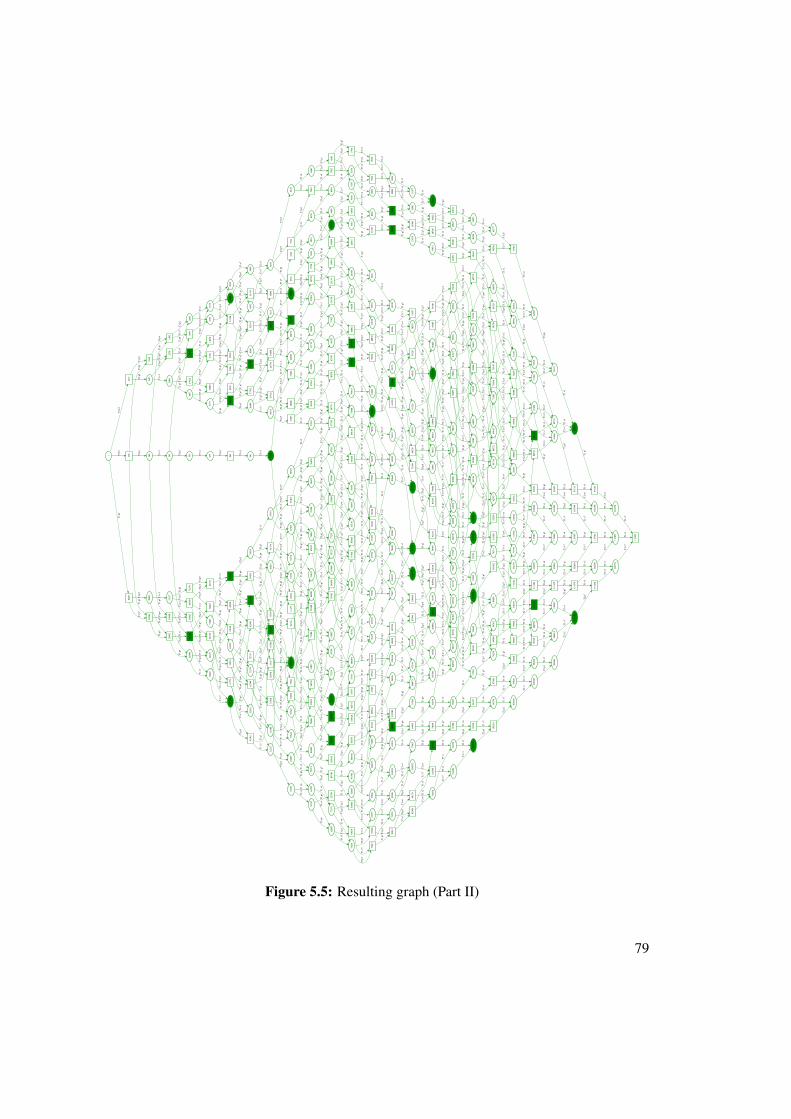
530
61
634
31T1.p
6
542
45
T2.p
2
531
90
T3.p
7
646
15
T2.p
2
635
60
T3.p
7
737
95
T1.v
5T1
.p6
543
74
T3.p
7
553
33
T2.v
1T1
.p6
T2.p
2
533
26
T3.p
4
315
29
419
01
T1.p
5
327
45
T2.p
1
431
17
T2.p
1
522
37T1.v
2T1
.p5
369
13
472
85
T1.p
5
380
66
T2.p
7
370
42
T3.p
7
474
14
T3.p
7
576
21T1.v
2
484
38
T2.p
7T1
.p5
392
02
T2.v
3T1
.p5
371
78
T3.p
4
1
104
33
T1.p
1
121
7
T2.p
1
130T3
.p7
208
33T1.p
2
105
62T3.p
7
240
1
T2.p
2
134
6
T3.p
7T1
.p1
T2.p
1
266T3
.p4
384
58
488
30
T1.p
5
395
94
T2.v
3
591
66
T1.v
2
499
66
T2.v
3T1
.p5
407
45T2.v
7
722
95
826
59
T1.v
5
723
91
T3.v
2
827
55
T3.v
2
930
28
T1.p
7T1
.v5
724
55
T3.v
1
693
0
173
62T1.p
1
806
6
T2.v
3
184
98
T2.v
3
277
62
T1.p
2T1
.p1
921
7
T2.v
7
753
71 857
40
T1.p
7
764
59
T2.v
1
868
28
T2.v
1
961
06
T1.v
6T1
.p7
776
27
T2.p
3
792
19
895
88
T1.p
7
803
72
T2.p
7
793
15
T3.v
2
896
84
T3.v
2
999
54
T1.v
6
804
68
T3.v
2
815
08
T2.v
3T1
.p7
T2.p
7
793
79T3.v
1
616
9
166
01
T1.p
1
732
2
T2.p
7
632
9
T3.p
2
177
54
T2.p
7
270
01T1.p
2T1
.p1
748
2
T3.p
2
845
8
T2.v
3T2
.p7
644
9
T3.v
4
749
79
T1.v
5
657
03
T2.v
1
647
44T3.p
7
751
08
T3.p
7
760
67
T2.v
1
853
48
T1.p
7
658
32T3.p
7T1
.v5
668
71
T2.p
3T2
.v1
T1.v
5
648
80
T3.p
4
630
79
734
43
T1.v
5
631
75
T3.v
2
735
39
T3.v
2
838
12
T1.p
7T1
.v5
632
39
T3.v
1
607
74
711
44
T1.p
6
619
25
T2.v
7
608
70
T3.v
2
T2.v
7
712
40
T3.v
2T1
.v5
T1.p
6
620
21T3.v
2T1
.p6
T2.v
7
609
34
T3.v
1
112
298
113
449
T2.v
7
112
418
T3.v
4
113
569
T3.v
4T2
.v7
112
610
T3.p
1
700
08
T1.v
5T2
.v3
701
04T3.v
2
T1.v
5T2
.v3
701
68T3.v
1
103
082
T1.v
7
103
202
T3.v
4
T1.v
7
103
394
T3.p
1
388
1 143
13
T1.p
1
504
9
T2.p
3
154
81T2.p
3T2
.v2
T1.p
1
108
466
109
586
T2.v
2
108
602
T3.p
4 109
722
T3.p
4T2
.v2
108
729
T3.v
7
546
37
650
07
T1.p
6
557
25
T2.v
1
T1.v
5
660
95
T2.v
1T1
.p6
568
93
T2.p
3
584
85
688
55
T1.p
6
596
38
T2.p
7
585
81T3.v
2
T1.v
5T2
.p7
689
51T3.v
2T2
.v3
T1.p
6
597
34
T3.v
2T1
.p6
T2.p
7
586
45T3.v
1
110
009
111
162
T2.p
7
110
129
T3.v
4
T2.v
3
111
282
T3.v
4T2
.p7
110
321
T3.p
1
288
98
T1.p
2
196
49
T2.v
7 300
49
T2.v
7T1
.v1
T1.p
2
197
78
T3.p
7
465
7
150
89
T1.p
1
577
7
T2.v
2
478
6
T3.p
7
162
09
T2.v
2
152
18
T3.p
7T2
.p7
T1.p
1
590
6
T3.p
7T1
.p1
T2.v
2
492
2
T3.p
4
715
60
819
24
T1.v
5
716
96
T3.p
4
820
60
T3.p
4T1
.v5
718
23
T3.v
7
113
857
113
921
T3.v
1
784
84
786
20
T3.p
4
787
47T3.v
7
200
41
304
41
T1.p
2
T1.v
1
938
66
104
233
T1.v
7
939
86T3.v
4
104
353
T3.v
4T1
.v7
941
78T3.p
1
534
53T1.v
2
T2.p
2
638
23
T1.p
6
623
44
727
08T1.v
5T2
.p1
624
80
T3.p
4
739
24
T2.p
1
728
44
T3.p
4T2
.p2
T1.v
5
636
96
T3.p
4T1
.v5
T2.p
1
626
07
T3.v
7
323
53 427
25T1.p
5
324
82
T3.p
7
T1.v
2
428
54
T3.p
7T1
.p5
326
18
T3.p
4
104
641
104
705
T3.v
1
105
921
T2.p
1
403
53
T1.v
1
301
78
T3.p
7
404
82
T3.p
7
507
25
T1.p
5T1
.v1
303
14
T3.p
4
108
25
212
25
T1.p
2
T1.v
1
T2.p
7
266
09
T1.p
2
163
38
T3.p
7
T1.v
1T2
.p7
267
38
T3.p
7T1
.p2
164
74
T3.p
4
823
47
927
16T1.p
7
824
67
T3.v
4
T1.v
6
928
36
T3.v
4T3
.p1
T1.p
7
761
96
773
64
T2.p
3
763
32
T3.p
4
T2.v
2
775
00T3.p
4T3
.v7
T2.p
3
111
570
112
706
T2.v
3
111
634
T3.v
1
T2.v
7
112
770
T3.v
1T2
.v3
281
54
T1.p
2
188
90
T2.v
3
T1.v
1
292
90
T2.v
3T2
.v7
T1.p
2
T1.v
1T2
.v7
311
37T1.v
1
209
62
T3.p
7
T2.p
1
312
66
T3.p
7
415
09
T1.p
5T1
.v1
210
98T3.p
4
160
9
279
3
T2.p
2
T2.v
1
892
76 996
42
T1.v
6
893
96
T3.v
4
T1.v
7
997
62
T3.v
4T3
.p1
T1.v
6
577
50
681
20
T1.p
6
578
86
T3.p
4
T1.v
5
682
56T3.p
4T1
.p6
580
13T3.v
7
931
24
103
490
T1.v
6 931
88T3.v
1
T1.v
7
103
554
T3.v
1T1
.v6
731
31 835
00
T1.p
7
732
51
T3.v
4
T1.v
6
836
20
T3.v
4T3
.p1
T1.p
7
T1.v
1T2
.v3
139
21
T2.p
3
140
50
T3.p
7
T2.p
3
141
86
T3.p
4
100
050
110
417
T1.v
7
100
114
T3.v
1
T2.p
7
110
481
T3.v
1T1
.v7
100
81
101
77T3.v
2
102
41
T3.v
1
800
60
811
96T2.v
3
801
80
T3.v
4
T2.v
7
813
16
T3.v
4T3
.p1
T2.v
3
708
32
T1.v
5
719
83T2.v
7
709
52
T3.v
4
T1.v
5
721
03
T3.v
4T3
.p1
T1.v
5T2
.v7
T2.p
7
373
05
T1.v
1
T2.p
7
476
77
T1.p
5
839
08
942
74
T1.v
6
839
72
T3.v
1 T1.v
7
943
38
T3.v
1T1
.v6
851
88
T2.p
1
106
210
107
298
T2.v
1
106
346
T3.p
4
T2.p
3
107
434
T3.p
4T2
.v1
106
473
T3.v
7
816
04
T2.v
7
816
68T3.v
1
T1.p
7
828
19
T3.v
1T2
.v7
616
13
T1.p
6
617
33
T3.v
4
T3.p
1T1
.p6
554
62
T1.p
6
566
30
T2.p
3
555
98
T3.p
4
T1.v
5
670
00
T2.p
3
659
68
T3.p
4T2
.v2
T1.p
6
567
66
T3.p
4T3
.v7
T1.p
6T2
.p3
348
9T2.v
1
253
0
T3.p
7
T2.p
3T1
.p1
361
8
T3.p
7T2
.v1
266
6
T3.p
4
865
961T3
.v2
102
5
T3.v
1
T1.v
5T2
.v2
671
36
T3.p
4
T1.v
5T2
.v2
672
63T3.v
7
508
54
611
90
T1.v
2
509
90
T3.p
4
T1.p
6
613
26
T3.p
4T1
.v2
511
17
T3.v
7
T2.p
2
740
60
T3.p
4
T2.v
1
752
44T3.p
4T2
.p2
741
87T3.v
7
T2.v
2
685
43
789
07
T1.v
5
696
96
T2.p
7
686
63
T3.v
4
T1.p
7T2
.p7
790
27
T3.v
4T1
.v5
T2.v
3
698
16
T3.v
4T3
.p1
T1.v
5T2
.p7
779
4
893
0
T2.v
3
789
0
T3.v
2
T2.v
7
902
6
T3.v
2T2
.v3
795
4
T3.v
1
523
97
627
67T1.p
6
525
17
T3.v
4 T1.v
5
628
87
T3.v
4T1
.p6
527
09
T3.p
1
T1.v
5
T1.v
6
897
48
T3.v
1T2
.v3
805
32
T3.v
1T1
.p7
T2.p
7
416
38
519
74T1.v
2T2
.p1
417
74
T3.p
4
T2.p
1T1
.p6
521
10
T3.p
4T1
.v2
429
90
T3.p
4T3
.v7
T1.v
2T2
.p1
593
26
T1.p
6
604
62
T2.v
3
594
46
T3.v
4
T1.p
6T2
.v7
605
82
T3.v
4T3
.p1
T1.p
6T2
.v3
T1.p
7
736
03
T3.v
1T1
.v5
644
55
T2.p
1
934
6
T1.p
1
948
2
T3.p
4
T1.p
2
199
14
T3.p
4T1
.p1
960
9
T3.v
7
113
162
113
289
T3.v
7
T3.p
2
T2.v
7T1
.v5
713
04
T3.v
1T1
.p6
620
85
T3.v
1T1
.p6
T2.v
7
107
105
T2.p
2
T1.v
5T2
.v3
T2.v
7
T1.p
6T2
.v1
545
10
T3.p
4T3
.v7
T1.p
6T2
.p2
T1.p
2
106
98T3.p
4T2
.p2
148
2
T3.p
4T1
.p1
T2.p
1
393T3
.v7
T1.v
2
475
50
T3.p
4T3
.v7
T1.p
5
103
946
105
162
T2.p
1
104
073
T3.v
7
T2.p
2
105
289
T3.v
7T3
.p2
T2.p
1
T1.v
5T2
.p7
690
15T3.v
1T2
.v3
T1.p
6
597
98
T3.v
1T1
.p6
T2.p
7
T1.v
7
113
761
T3.p
1T3
.v2
T2.v
7T2
.p7
T3.v
7T2
.v1
T1.v
5
T1.v
7
955
54
T2.p
1T1
.v6
863
72
T2.p
2
T1.p
7T3
.v2
T1.v
7
861
8
976
9
T2.v
7
873
8
T3.v
4
988
9
T3.v
4T3
.p1
T2.v
7
T2.v
3
111
474
T3.p
1T3
.v2
T2.p
7
978
26
108
193
T1.v
7
989
94
T2.p
3 109
361
T2.p
3T2
.v2
T1.v
7
T2.v
2
104
545T3
.p1
T3.v
2T1
.v7
T2.v
2
153
54
T3.p
4T1
.p1
604
2
T3.p
4T3
.v7
T1.p
1T2
.v2
T1.v
6T2
.v3
109
849
T3.v
7T2
.v2
T2.v
3
760
2
T3.v
4T2
.p7
664
1
T3.p
1
821
87
T3.v
7T3
.p2
T1.v
5
206
73
T1.p
1
T1.p
7
748
19
T2.p
1T1
.v5
656
39
T2.p
2T3
.p2
891
16
T1.p
7
799
00
T2.p
7
T1.v
5T2
.v7
T1.p
6T1
.v6
T3.p
1
T3.v
7T1
.p5
T1.p
5
406
18
T3.p
4T3
.v7
T1.v
1
T1.v
1
268
74
T3.p
4T3
.v7
T1.p
2
T2.p
1
729
71
T3.v
7T1
.v5
T2.p
2T3
.v7
T3.p
2T1
.v5
T2.p
1
770
91
874
60
T1.p
7
782
59
T2.p
3
T1.v
6
886
28
T2.p
3T2
.v2
T1.p
7T1
.v7
T3.p
1
114
57
T1.p
1
224
1
T2.p
1
T1.v
6T2
.v2
T1.v
6T3
.p1
T1.v
7
967
38
T2.p
2
T2.v
1T1
.v7
T2.p
1T1
.p5
314
02
T3.p
4T3
.v7
T1.v
1
T2.v
7
909
0
T3.v
1
183
86
T1.p
1T2
.v3
T1.v
5T2
.p7
T2.v
3T1
.p6
T2.v
2T3
.v7
T2.v
7T3
.p1
T3.p
1T1
.v5
T3.v
7T2
.p3
T1.v
5
683
83T3.v
7T1
.p6
T2.p
7
581
73
T3.p
2
T2.v
1
563
57
667
27
T1.p
6
575
25
T2.p
3
T1.v
5
678
95
T2.p
3T2
.v2
T1.p
6T3
.p1
T1.p
7T2
.p7
T3.p
1T1
.v5
T2.v
3
T1.v
5T2
.v2
T2.p
3T1
.p1
375
4
T3.p
4T3
.v7
T2.v
1
T2.p
3
107
561
T3.v
7T2
.v1
T3.p
1T1
.v5
T1.p
6
528
05
T3.v
2
T1.p
7
760
03
T2.p
2
T2.v
1T1
.p7
517
49
T1.v
2
T1.v
5T2
.p3
T3.v
7T2
.v2
T1.p
6T3
.v7
T3.p
1T1
.p6
T2.v
7
T1.v
5T2
.v2
T3.v
7T2
.v1
T2.p
2
845
56
T1.p
7
T1.p
6
614
53
T3.v
7T1
.v2
402
26
505
98
T1.p
5
413
77
T2.v
7
T1.v
2T2
.v7
T1.p
5
425
33
528
69
T1.v
2
437
49
T2.p
1
T1.p
6
540
85
T2.p
1T1
.v2
111
746
112
897
T2.v
7
113
026
T3.p
7
310
73
T1.p
2
T2.v
1T1
.v6
494
62
T1.v
2T2
.v3
T1.p
6T2
.p1
T3.v
7T3
.v7
T1.v
2
102
530
T1.v
7
T3.v
7T1
.p2
T1.p
1T3
.p2
T1.p
6
552
69
T2.p
2
T2.v
1T1
.p6
218
57
T1.p
2
342
5
T2.p
2
379
37
483
09
T1.p
5
390
90
T2.p
7
T1.v
2T2
.p7
T2.v
3T1
.p5
T2.p
2
109
457
T3.p
7 110
610
T2.p
7
T2.v
3
195
22
T2.v
3
287
86
T1.p
2T2
.v7
T1.p
1
933
14
103
681
T1.v
7
945
30
T2.p
1
104
897
T2.p
1
103
810
T3.p
7T1
.v7
957
14
T2.p
2
T3.v
7T2
.v1
T1.p
6
T3.v
7T1
.p2
T3.v
7T2
.p2
T1.p
1T2
.p1
553T3
.p2
T1.v
2T3
.v7
111
002
T3.p
2
112
138
T2.v
3
T3.p
2T2
.v7
T2.v
1T1
.v5
925
56
T3.p
2
102
922
T1.v
6
T3.p
2T1
.v7
107
169
T3.p
7
108
337
T2.p
3
T3.p
7T2
.v2
T3.p
1
994
82
T3.p
2T1
.v7
T3.p
2T2
.p7
817
95
T3.p
7
921
64
T1.p
7
T1.v
6
833
40
T3.p
2
937
06T1.v
6T2
.p1
T3.p
2T1
.v7
949
22
T2.p
1T2
.p2
T1.v
6
887
24
990
90
T1.v
6
T1.v
7
810
36
T3.p
2T2
.v7
T3.p
2T1
.p7
725
79
T3.p
7
829
48
T1.p
7T2
.p1
T1.v
6
841
64
T2.p
1T2
.p2
T3.p
7T1
.p7
T3.p
1T2
.v3
T2.p
7
673
7
T3.v
2
T2.v
7
299
22
T1.p
2
T1.v
1T2
.v7
568
1
161
13
T1.p
1
680
1
T2.v
2
172
33T2.v
2T2
.p7
T1.p
1
971
94
T1.v
7
983
62
T2.p
3
T2.p
3T1
.v7
T2.v
2
702
80
806
44
T1.v
5
714
31
T2.v
7
T2.v
7T3
.p7
T1.v
5
795
08 T2.v
3
979
70
T1.v
7T2
.v2
T3.v
7T2
.v2
T3.v
7T1
.p1
864
36
968
02
T1.v
6
876
04
T2.p
3
T1.v
7T2
.p3
T2.v
2T1
.v6
T3.p
2T1
.v6
T3.p
2T2
.v3
610
61
T3.p
7T1
.p6
333
77
T1.p
5
T1.v
1
106
081
T2.p
2
105
026
T3.p
7
T3.p
7T2
.v1
T2.p
2T3
.p4
T2.p
7
276
33
T1.p
2
T1.v
1T2
.p7
T3.p
2T2
.p1
T1.p
7T2
.p2
T1.v
5
679
91
T3.p
7
783
55
T1.v
5
691
44
T2.p
7
T3.p
7T1
.p7
T2.p
7T2
.v3
T1.v
5
603
02
T3.p
2
706
72
T1.p
6T2
.v7
T3.p
2T2
.v7
T1.v
5T3
.p2
T1.p
6
518
45
T2.p
1T3
.p7 622
15
T1.p
6
T2.p
1T3
.p7
T1.v
5
T1.p
5T3
.v7
T3.v
7T1
.v1
321
61
T1.v
1
T1.p
5T2
.p1
695
36
T3.p
2T1
.v5
T2.v
3
T1.v
6
879
96
T2.p
3T2
.v2
T1.p
7
T1.v
6T2
.v2
587
74
T1.p
6
599
10
T2.v
3
T1.p
6T2
.v7
T1.v
1T2
.v3
149
45
T2.p
3
772
35
T3.p
7T1
.p7
T2.v
2
T3.v
7T1
.p5
T2.p
1
T1.v
7T2
.p2
T1.v
7T2
.v1
T3.v
2
T3.p
7T1
.p7
T2.p
3T3
.p7
T2.v
2T1
.v5
T3.p
2T1
.v5
T2.p
7T3
.p2
T2.v
3T1
.p6
T1.p
6T2
.p7
582
93T3.v
4
T1.v
6T2
.p2
T2.v
1T1
.v6
451
3
T2.v
1
T2.p
3T1
.p1
T3.v
2T2
.v3
T1.v
5T2
.p3
T2.v
2T1
.p6
495
74 T1.v
2T2
.v7
T3.p
7T1
.v2
T2.v
1T1
.v7
T3.v
7T2
.p3
T1.p
1
T3.v
2
565
01
T3.p
7T1
.p6
T2.v
2
T3.p
7T1
.p6
T2.p
7
T2.v
7T1
.v2
T1.p
5
T2.p
1T3
.p2
T1.p
6T1
.p1
T3.p
7
T1.v
2T2
.v3
T3.v
2T1
.v6
T2.p
1T3
.p7
T1.v
2
T3.v
2T1
.v7
T2.v
7T1
.p5
T3.v
2T1
.v6
T2.p
7T1
.v2
673T3
.v4
T2.v
7T3
.v2
T1.p
1T3
.p2
T2.v
7
T1.p
6T3
.p7
T2.p
3
T1.p
6T3
.v1
T2.p
7T3
.v1
T3.p
1T1
.p6
T2.p
7
T3.p
1
T3.p
4
T3.p
4T2
.p1
Figure 5.5: Resulting graph (Part II)
79
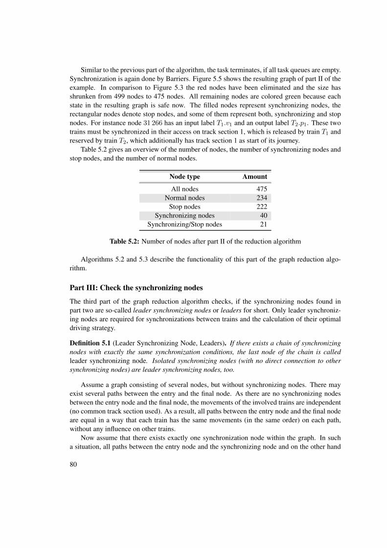
Similar to the previous part of the algorithm, the task terminates, if all task queues are empty.Synchronization is again done by Barriers. Figure 5.5 shows the resulting graph of part II of theexample. In comparison to Figure 5.3 the red nodes have been eliminated and the size hasshrunken from 499 nodes to 475 nodes. All remaining nodes are colored green because eachstate in the resulting graph is safe now. The filled nodes represent synchronizing nodes, therectangular nodes denote stop nodes, and some of them represent both, synchronizing and stopnodes. For instance node 31 266 has an input label T1.v1 and an output label T2.p1. These twotrains must be synchronized in their access on track section 1, which is released by train T1 andreserved by train T2, which additionally has track section 1 as start of its journey.
Table 5.2 gives an overview of the number of nodes, the number of synchronizing nodes andstop nodes, and the number of normal nodes.
Node type Amount
All nodes 475Normal nodes 234
Stop nodes 222Synchronizing nodes 40
Synchronizing/Stop nodes 21
Table 5.2: Number of nodes after part II of the reduction algorithm
Algorithms 5.2 and 5.3 describe the functionality of this part of the graph reduction algo-rithm.
Part III: Check the synchronizing nodes
The third part of the graph reduction algorithm checks, if the synchronizing nodes found inpart two are so-called leader synchronizing nodes or leaders for short. Only leader synchroniz-ing nodes are required for synchronizations between trains and the calculation of their optimaldriving strategy.
Definition 5.1 (Leader Synchronizing Node, Leaders). If there exists a chain of synchronizingnodes with exactly the same synchronization conditions, the last node of the chain is calledleader synchronizing node. Isolated synchronizing nodes (with no direct connection to othersynchronizing nodes) are leader synchronizing nodes, too.
Assume a graph consisting of several nodes, but without synchronizing nodes. There mayexist several paths between the entry and the final node. As there are no synchronizing nodesbetween the entry node and the final node, the movements of the involved trains are independent(no common track section used). As a result, all paths between the entry node and the final nodeare equal in a way that each train has the same movements (in the same order) on each path,without any influence on other trains.
Now assume that there exists exactly one synchronization node within the graph. In sucha situation, all paths between the entry node and the synchronizing node and on the other hand
80
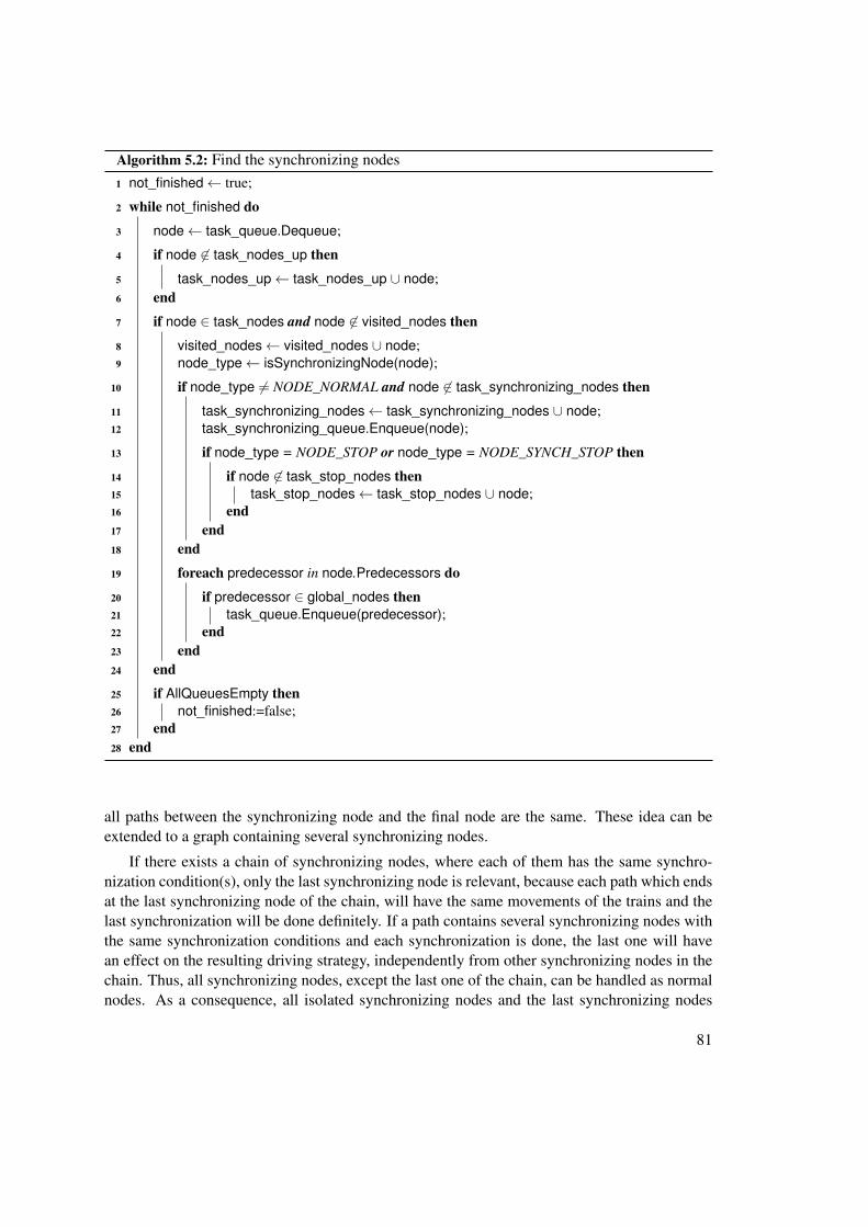
Algorithm 5.2: Find the synchronizing nodes1 not_finished← true;
2 while not_finished do
3 node← task_queue.Dequeue;
4 if node 6∈ task_nodes_up then
5 task_nodes_up← task_nodes_up ∪ node;6 end
7 if node ∈ task_nodes and node 6∈ visited_nodes then
8 visited_nodes← visited_nodes ∪ node;9 node_type← isSynchronizingNode(node);
10 if node_type 6= NODE_NORMAL and node 6∈ task_synchronizing_nodes then
11 task_synchronizing_nodes← task_synchronizing_nodes ∪ node;12 task_synchronizing_queue.Enqueue(node);
13 if node_type = NODE_STOP or node_type = NODE_SYNCH_STOP then
14 if node 6∈ task_stop_nodes then15 task_stop_nodes← task_stop_nodes ∪ node;16 end17 end18 end
19 foreach predecessor in node.Predecessors do
20 if predecessor ∈ global_nodes then21 task_queue.Enqueue(predecessor);22 end23 end24 end
25 if AllQueuesEmpty then26 not_finished:=false;27 end28 end
all paths between the synchronizing node and the final node are the same. These idea can beextended to a graph containing several synchronizing nodes.
If there exists a chain of synchronizing nodes, where each of them has the same synchro-nization condition(s), only the last synchronizing node is relevant, because each path which endsat the last synchronizing node of the chain, will have the same movements of the trains and thelast synchronization will be done definitely. If a path contains several synchronizing nodes withthe same synchronization conditions and each synchronization is done, the last one will havean effect on the resulting driving strategy, independently from other synchronizing nodes in thechain. Thus, all synchronizing nodes, except the last one of the chain, can be handled as normalnodes. As a consequence, all isolated synchronizing nodes and the last synchronizing nodes
81

Algorithm 5.3: Check the synchronizing nodes: isSynchronizingNode1 result← NODE_NORMAL;
2 foreach predecessor in node.Predecessors do
3 if node ∈ global_nodes then
4 if node.t_departure > 0 then5 result← NODE_STOP;6 end7 end8 end
9 foreach successor in node.Successors do
10 if successor ∈ global_nodes then
11 label_successor← EdgeLabelSection(node,successor);
12 if label_successor = p then
13 foreach predecessor in node.Predecessors do
14 if predecessor ∈ global_nodes then
15 label_predecessor← EdgeLabelSection(predecessor,node);
16 if label_predecessor = v then
17 if label_successor = label_predecessor then
18 if result = NODE_STOP then19 result← NODE_SYNCH_STOP;20 else21 result← NODE_SYNCH;22 end
23 CreateSynchronizationCondition;24 end25 end26 end27 end28 end29 end30 end
of a chain will be handled as leaders, the others will be handled as non-synchronizing nodes.The entry node and the final node are generally handled as synchronizing nodes, in particular asleader synchronizing nodes. As stop nodes are a special kind of synchronizing nodes, this partof the algorithm is applied in the same way for both synchronizing nodes and stop nodes. Dueto simplification only the term synchronizing nodes will be used in the explanation.
Example 5.2. Figure 5.6 shows an example with three synchronizing nodes, namely node 5, 8,and 11. Train n and train m are involved in the synchronization on track section k. The threementioned synchronizing nodes form a chain, where each node of them has the same synchro-
82
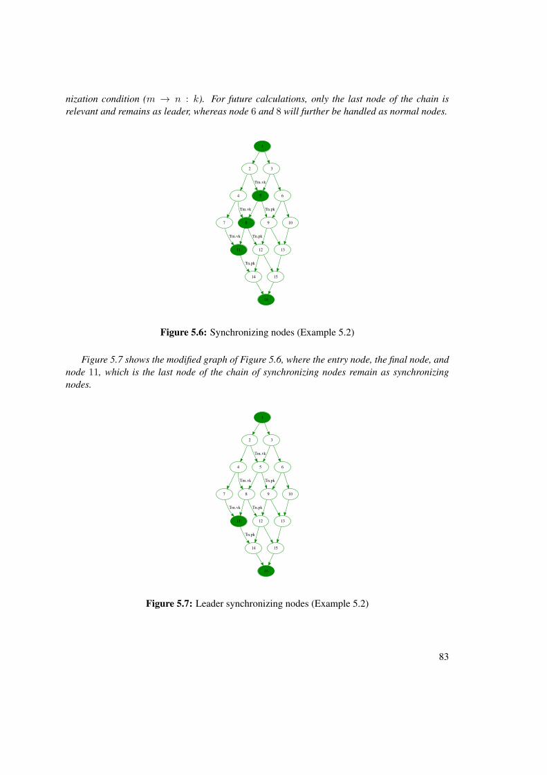
nization condition (m → n : k). For future calculations, only the last node of the chain isrelevant and remains as leader, whereas node 6 and 8 will further be handled as normal nodes.
1
2 3
4 5
Tm.vk
6
7 8
Tm.vk
9
Tn.pk
10
11
Tm.vk
12
Tn.pk
13
14
Tn.pk
15
16
Figure 5.6: Synchronizing nodes (Example 5.2)
Figure 5.7 shows the modified graph of Figure 5.6, where the entry node, the final node, andnode 11, which is the last node of the chain of synchronizing nodes remain as synchronizingnodes.
1
2 3
4 5
Tm.vk
6
7 8
Tm.vk
9
Tn.pk
10
11
Tm.vk
12
Tn.pk
13
14
Tn.pk
15
16
Figure 5.7: Leader synchronizing nodes (Example 5.2)
83
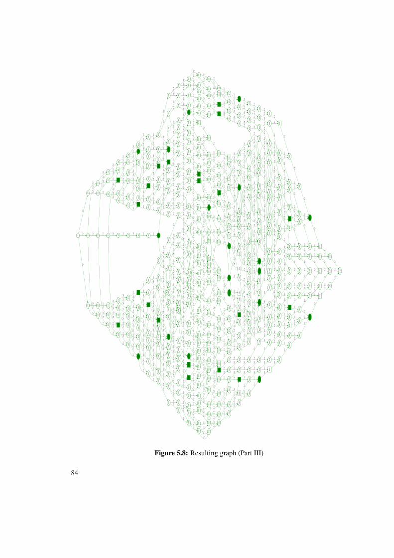
530
61
634
31T1.
p6
542
45
T2.
p2
531
90
T3.
p7
646
15
T2.
p2
635
60
T3.
p7
737
95
T1.
v5T
1.p6
543
74
T3.
p7
553
33
T2.
v1T
1.p6
T2.
p2
533
26
T3.
p4
315
29
419
01
T1.
p5
327
45
T2.
p1
431
17
T2.
p1
522
37T1.
v2T
1.p5
369
13
472
85
T1.
p5
380
66
T2.
p7
370
42
T3.
p7
474
14
T3.
p7
576
21T1.
v2
484
38
T2.
p7T
1.p5
392
02
T2.
v3T
1.p5
371
78
T3.
p4
1
104
33
T1.
p1
121
7
T2.
p1
130T
3.p7
208
33T1.
p2
105
62T3.
p7
240
1
T2.
p2
134
6
T3.
p7T
1.p1
T2.
p1
266T
3.p4
384
58
488
30
T1.
p5
395
94T2.
v3
591
66
T1.
v2
499
66
T2.
v3T
1.p5
407
45
T2.
v7
722
95
826
59
T1.
v5
723
91
T3.
v2
827
55
T3.
v2
930
28
T1.
p7T
1.v5
724
55
T3.
v1
693
0
173
62T1.
p1
806
6
T2.
v3
184
98
T2.
v3
277
62
T1.
p2T
1.p1
921
7
T2.
v7
753
71
857
40T1.
p7
764
59
T2.
v1
868
28
T2.
v1
961
06
T1.
v6T
1.p7
776
27
T2.
p3
792
19
895
88
T1.
p7
803
72
T2.
p7
793
15
T3.
v2
896
84
T3.
v2
999
54
T1.
v6
804
68
T3.
v2
815
08
T2.
v3T
1.p7
T2.
p7
793
79
T3.
v1
616
9
166
01
T1.
p1
732
2
T2.
p7
632
9
T3.
p2
177
54
T2.
p7
270
01
T1.
p2T
1.p1
748
2
T3.
p2
845
8
T2.
v3T
2.p7
644
9
T3.
v4
749
79
T1.
v5
657
03
T2.
v1
647
44T3.
p7
751
08
T3.
p7
760
67T2.
v1
853
48
T1.
p7
658
32T3.
p7T
1.v5
668
71
T2.
p3T
2.v1
T1.
v5
648
80
T3.
p4
630
79
734
43
T1.
v5
631
75
T3.
v2
735
39
T3.
v2
838
12
T1.
p7T
1.v5
632
39
T3.
v1
607
74
711
44
T1.
p6
619
25
T2.
v7
608
70
T3.
v2
T2.
v7
712
40
T3.
v2T
1.v5
T1.
p6
620
21T3.
v2T
1.p6
T2.
v7
609
34
T3.
v1
112
298
113
449
T2.
v7
112
418
T3.
v4
113
569
T3.
v4T
2.v7
112
610
T3.
p1
700
08
T1.
v5T
2.v3
701
04T3.
v2
T1.
v5T
2.v3
701
68T3.
v1
103
082
T1.
v7
103
202
T3.
v4
T1.
v7
103
394
T3.
p1
388
1 143
13
T1.
p1
504
9
T2.
p3
154
81T2.
p3T
2.v2
T1.
p1
108
466
109
586
T2.
v2
108
602
T3.
p4
109
722
T3.
p4T
2.v2
108
729
T3.
v7
546
37
650
07
T1.
p6
557
25
T2.
v1
T1.
v5
660
95
T2.
v1T
1.p6
568
93
T2.
p3
584
85
688
55
T1.
p6
596
38
T2.
p7
585
81
T3.
v2
T1.
v5T
2.p7
689
51T3.
v2T
2.v3
T1.
p6
597
34
T3.
v2T
1.p6
T2.
p7
586
45T3.
v1
110
009
111
162
T2.
p7
110
129
T3.
v4
T2.
v3
111
282
T3.
v4T
2.p7
110
321
T3.
p1
288
98T1.
p2
196
49
T2.
v7
300
49
T2.
v7T
1.v1
T1.
p2
197
78
T3.
p7
465
7
150
89
T1.
p1
577
7
T2.
v2
478
6
T3.
p7
162
09
T2.
v2
152
18
T3.
p7T
2.p7
T1.
p1
590
6
T3.
p7T
1.p1
T2.
v2
492
2
T3.
p4
715
60
819
24
T1.
v5
716
96
T3.
p4
820
60
T3.
p4T
1.v5
718
23
T3.
v7
113
857
113
921
T3.
v1
784
84
786
20
T3.
p4
787
47T3.
v7
200
41
304
41
T1.
p2
T1.
v1
938
66
104
233
T1.
v7
939
86T3.
v4
104
353
T3.
v4T
1.v7
941
78T3.
p1
534
53T1.
v2
T2.
p2
638
23
T1.
p6
623
44
727
08T1.
v5T
2.p1
624
80
T3.
p4
739
24
T2.
p1
728
44
T3.
p4T
2.p2
T1.
v5
636
96
T3.
p4T
1.v5
T2.
p1
626
07
T3.
v7
323
53 427
25T1.
p5
324
82
T3.
p7
T1.
v2
428
54
T3.
p7T
1.p5
326
18
T3.
p4
104
641
104
705
T3.
v1
105
921
T2.
p1
403
53
T1.
v1
301
78
T3.
p7
404
82
T3.
p7
507
25
T1.
p5T
1.v1
303
14
T3.
p4
108
25
212
25
T1.
p2
T1.
v1
T2.
p7
266
09
T1.
p2
163
38
T3.
p7
T1.
v1T
2.p7
267
38
T3.
p7T
1.p2
164
74
T3.
p4
823
47
927
16T1.
p7
824
67
T3.
v4
T1.
v6
928
36
T3.
v4T
3.p1
T1.
p7
761
96
773
64
T2.
p3
763
32
T3.
p4
T2.
v2
775
00T3.
p4T
3.v7
T2.
p3
111
570
112
706
T2.
v3
111
634
T3.
v1
T2.
v7
112
770
T3.
v1T
2.v3
281
54
T1.
p2
188
90
T2.
v3
T1.
v1
292
90
T2.
v3T
2.v7
T1.
p2
T1.
v1T
2.v7
311
37T1.
v1
209
62
T3.
p7
T2.
p1
312
66
T3.
p7
415
09
T1.
p5T
1.v1
210
98T3.
p4
160
9
279
3
T2.
p2
T2.
v1
892
76
996
42
T1.
v6
893
96
T3.
v4
T1.
v7
997
62
T3.
v4T
3.p1
T1.
v6
577
50
681
20
T1.
p6
578
86
T3.
p4
T1.
v5
682
56T3.
p4T
1.p6
580
13T3.
v7
931
24
103
490
T1.
v6
931
88T3.
v1
T1.
v7
103
554
T3.
v1T
1.v6
731
31 835
00
T1.
p7
732
51
T3.
v4
T1.
v6
836
20
T3.
v4T
3.p1
T1.
p7
T1.
v1T
2.v3
139
21
T2.
p3
140
50
T3.
p7
T2.
p3
141
86
T3.
p4
100
050
110
417
T1.
v7
100
114
T3.
v1
T2.
p7
110
481
T3.
v1T
1.v7
100
81
101
77
T3.
v2
102
41
T3.
v1
800
60
811
96T2.
v3
801
80
T3.
v4
T2.
v7
813
16
T3.
v4T
3.p1
T2.
v3
708
32
T1.
v5
719
83T2.
v7
709
52
T3.
v4
T1.
v5
721
03
T3.
v4T
3.p1
T1.
v5T
2.v7
T2.
p7
373
05
T1.
v1
T2.
p7
476
77
T1.
p5
839
08
942
74
T1.
v6
839
72
T3.
v1 T1.
v7
943
38
T3.
v1T
1.v6
851
88
T2.
p1
106
210
107
298
T2.
v1
106
346
T3.
p4
T2.
p3
107
434
T3.
p4T
2.v1
106
473
T3.
v7
816
04
T2.
v7
816
68
T3.
v1
T1.
p7
828
19
T3.
v1T
2.v7
616
13
T1.
p6
617
33
T3.
v4
T3.
p1T
1.p6
554
62
T1.
p6
566
30
T2.
p3
555
98
T3.
p4
T1.
v5
670
00
T2.
p3
659
68
T3.
p4T
2.v2
T1.
p6
567
66
T3.
p4T
3.v7
T1.
p6T
2.p3
348
9T2.
v1
253
0
T3.
p7
T2.
p3T
1.p1
361
8
T3.
p7T
2.v1
266
6
T3.
p4
865
961T
3.v2
102
5
T3.
v1
T1.
v5T
2.v2
671
36
T3.
p4
T1.
v5T
2.v2
672
63T3.
v7
508
54
611
90
T1.
v2
509
90
T3.
p4
T1.
p6
613
26
T3.
p4T
1.v2
511
17
T3.
v7
T2.
p2
740
60
T3.
p4
T2.
v1
752
44T3.
p4T
2.p2
741
87T3.
v7
T2.
v2
685
43
789
07
T1.
v5
696
96
T2.
p7
686
63
T3.
v4
T1.
p7T
2.p7
790
27
T3.
v4T
1.v5
T2.
v3
698
16
T3.
v4T
3.p1
T1.
v5T
2.p7
779
4
893
0
T2.
v3
789
0
T3.
v2
T2.
v7
902
6
T3.
v2T
2.v3
795
4
T3.
v1
523
97
627
67T1.
p6
525
17
T3.
v4 T1.
v5
628
87
T3.
v4T
1.p6
527
09
T3.
p1
T1.
v5
T1.
v6
897
48T3.
v1T
2.v3
805
32
T3.
v1T
1.p7
T2.
p7
416
38
519
74T1.
v2T
2.p1
417
74
T3.
p4
T2.
p1T
1.p6
521
10
T3.
p4T
1.v2
429
90
T3.
p4T
3.v7
T1.
v2T
2.p1
593
26
T1.
p6
604
62
T2.
v3
594
46
T3.
v4
T1.
p6T
2.v7
605
82
T3.
v4T
3.p1
T1.
p6T
2.v3
T1.
p7
736
03
T3.
v1T
1.v5
644
55
T2.
p1
934
6
T1.
p1
948
2
T3.
p4
T1.
p2
199
14
T3.
p4T
1.p1
960
9
T3.
v7
113
162
113
289
T3.
v7
T3.
p2
T2.
v7T
1.v5
713
04
T3.
v1T
1.p6
620
85
T3.
v1T
1.p6
T2.
v7
107
105
T2.
p2
T1.
v5T
2.v3
T2.
v7
T1.
p6T
2.v1
545
10
T3.
p4T
3.v7
T1.
p6T
2.p2
T1.
p2
106
98T3.
p4T
2.p2
148
2
T3.
p4T
1.p1
T2.
p1
393T
3.v7
T1.
v2
475
50
T3.
p4T
3.v7
T1.
p5
103
946
105
162
T2.
p1
104
073
T3.
v7
T2.
p2
105
289
T3.
v7T
3.p2
T2.
p1
T1.
v5T
2.p7
690
15T3.
v1T
2.v3
T1.
p6
597
98
T3.
v1T
1.p6
T2.
p7
T1.
v7
113
761
T3.
p1T
3.v2
T2.
v7T
2.p7
T3.
v7T
2.v1
T1.
v5
T1.
v7
955
54
T2.
p1T
1.v6
863
72
T2.
p2
T1.
p7T
3.v2
T1.
v7
861
8
976
9
T2.
v7
873
8
T3.
v4
988
9
T3.
v4T
3.p1
T2.
v7
T2.
v3
111
474
T3.
p1T
3.v2
T2.
p7
978
26
108
193
T1.
v7
989
94
T2.
p3 109
361
T2.
p3T
2.v2
T1.
v7
T2.
v2
104
545
T3.
p1T
3.v2
T1.
v7
T2.
v2
153
54
T3.
p4T
1.p1
604
2
T3.
p4T
3.v7
T1.
p1T
2.v2
T1.
v6T
2.v3
109
849
T3.
v7T
2.v2
T2.
v3
760
2
T3.
v4T
2.p7
664
1
T3.
p1
821
87
T3.
v7T
3.p2
T1.
v5
206
73
T1.
p1
T1.
p7
748
19
T2.
p1T
1.v5
656
39
T2.
p2T
3.p2
891
16
T1.
p7
799
00
T2.
p7
T1.
v5T
2.v7
T1.
p6T
1.v6
T3.
p1
T3.
v7T
1.p5
T1.
p5
406
18
T3.
p4T
3.v7
T1.
v1
T1.
v1
268
74
T3.
p4T
3.v7
T1.
p2
T2.
p1
729
71
T3.
v7T
1.v5
T2.
p2T
3.v7
T3.
p2T
1.v5
T2.
p1
770
91
874
60T1.
p7
782
59
T2.
p3
T1.
v6
886
28
T2.
p3T
2.v2
T1.
p7T
1.v7
T3.
p1
114
57
T1.
p1
224
1
T2.
p1
T1.
v6T
2.v2
T1.
v6T
3.p1
T1.
v7
967
38
T2.
p2
T2.
v1T
1.v7
T2.
p1T
1.p5
314
02
T3.
p4T
3.v7
T1.
v1
T2.
v7
909
0
T3.
v1
183
86
T1.
p1T
2.v3
T1.
v5T
2.p7
T2.
v3T
1.p6
T2.
v2T
3.v7
T2.
v7T
3.p1
T3.
p1T
1.v5
T3.
v7T
2.p3
T1.
v5
683
83T3.
v7T
1.p6
T2.
p7
581
73
T3.
p2
T2.
v1
563
57
667
27
T1.
p6
575
25
T2.
p3
T1.
v5
678
95
T2.
p3T
2.v2
T1.
p6T
3.p1
T1.
p7T
2.p7
T3.
p1T
1.v5
T2.
v3
T1.
v5T
2.v2
T2.
p3T
1.p1
375
4
T3.
p4T
3.v7
T2.
v1
T2.
p3
107
561
T3.
v7T
2.v1
T3.
p1T
1.v5
T1.
p6
528
05
T3.
v2
T1.
p7
760
03
T2.
p2
T2.
v1T
1.p7
517
49
T1.
v2
T1.
v5T
2.p3
T3.
v7T
2.v2
T1.
p6T
3.v7
T3.
p1T
1.p6
T2.
v7
T1.
v5T
2.v2
T3.
v7T
2.v1
T2.
p2
845
56
T1.
p7
T1.
p6
614
53
T3.
v7T
1.v2
402
26
505
98
T1.
p5
413
77
T2.
v7
T1.
v2T
2.v7
T1.
p5
425
33
528
69
T1.
v2
437
49
T2.
p1
T1.
p6
540
85
T2.
p1T
1.v2
111
746
112
897
T2.
v7
113
026
T3.
p7
310
73
T1.
p2
T2.
v1T
1.v6
494
62
T1.
v2T
2.v3
T1.
p6T
2.p1
T3.
v7T
3.v7
T1.
v2
102
530
T1.
v7
T3.
v7T
1.p2
T1.
p1T
3.p2
T1.
p6
552
69
T2.
p2
T2.
v1T
1.p6
218
57
T1.
p2
342
5
T2.
p2
379
37
483
09
T1.
p5
390
90
T2.
p7
T1.
v2T
2.p7
T2.
v3T
1.p5
T2.
p2
109
457
T3.
p7 110
610
T2.
p7
T2.
v3
195
22
T2.
v3
287
86
T1.
p2T
2.v7
T1.
p1
933
14
103
681
T1.
v7
945
30
T2.
p1
104
897
T2.
p1
103
810
T3.
p7T
1.v7
957
14
T2.
p2
T3.
v7T
2.v1
T1.
p6
T3.
v7T
1.p2
T3.
v7T
2.p2
T1.
p1T
2.p1
553T
3.p2
T1.
v2T
3.v7
111
002
T3.
p2
112
138T
2.v3
T3.
p2T
2.v7
T2.
v1T
1.v5
925
56
T3.
p2
102
922
T1.
v6
T3.
p2T
1.v7
107
169
T3.
p7
108
337
T2.
p3
T3.
p7T
2.v2
T3.
p1
994
82
T3.
p2T
1.v7
T3.
p2T
2.p7
817
95
T3.
p7
921
64
T1.
p7
T1.
v6
833
40
T3.
p2
937
06T1.
v6T
2.p1
T3.
p2T
1.v7
949
22
T2.
p1T
2.p2
T1.
v6
887
24
990
90
T1.
v6
T1.
v7
810
36
T3.
p2T
2.v7
T3.
p2T
1.p7
725
79
T3.
p7
829
48
T1.
p7T
2.p1
T1.
v6
841
64
T2.
p1T
2.p2
T3.
p7T
1.p7
T3.
p1T
2.v3
T2.
p7
673
7
T3.
v2
T2.
v7
299
22
T1.
p2
T1.
v1T
2.v7
568
1
161
13
T1.
p1
680
1
T2.
v2
172
33
T2.
v2T
2.p7
T1.
p1
971
94
T1.
v7
983
62
T2.
p3
T2.
p3T
1.v7
T2.
v2
702
80
806
44
T1.
v5
714
31T2.
v7
T2.
v7T
3.p7
T1.
v5
795
08 T2.
v3
979
70
T1.
v7T
2.v2
T3.
v7T
2.v2
T3.
v7T
1.p1
864
36
968
02
T1.
v6
876
04
T2.
p3
T1.
v7T
2.p3
T2.
v2T
1.v6
T3.
p2T
1.v6
T3.
p2T
2.v3
610
61
T3.
p7T
1.p6
333
77
T1.
p5
T1.
v1
106
081
T2.
p2
105
026
T3.
p7
T3.
p7T
2.v1
T2.
p2T
3.p4
T2.
p7
276
33
T1.
p2
T1.
v1T
2.p7
T3.
p2T
2.p1
T1.
p7T
2.p2
T1.
v5
679
91
T3.
p7
783
55
T1.
v5
691
44
T2.
p7
T3.
p7T
1.p7
T2.
p7T
2.v3
T1.
v5
603
02
T3.
p2
706
72
T1.
p6T
2.v7
T3.
p2T
2.v7
T1.
v5T
3.p2
T1.
p6
518
45
T2.
p1T
3.p7 6
2215
T1.
p6
T2.
p1T
3.p7
T1.
v5
T1.
p5T
3.v7
T3.
v7T
1.v1
321
61
T1.
v1
T1.
p5T
2.p1
695
36
T3.
p2T
1.v5
T2.
v3
T1.
v6
879
96
T2.
p3T
2.v2
T1.
p7
T1.
v6T
2.v2
587
74
T1.
p6
599
10
T2.
v3
T1.
p6T
2.v7
T1.
v1T
2.v3
149
45
T2.
p3
772
35
T3.
p7T
1.p7
T2.
v2
T3.
v7T
1.p5
T2.
p1
T1.
v7T
2.p2
T1.
v7T
2.v1
T3.
v2
T3.
p7T
1.p7
T2.
p3T
3.p7
T2.
v2T
1.v5
T3.
p2T
1.v5
T2.
p7T
3.p2
T2.
v3T
1.p6
T1.
p6T
2.p7
582
93T3.
v4
T1.
v6T
2.p2 T
2.v1
T1.
v6
451
3
T2.
v1
T2.
p3T
1.p1
T3.
v2T
2.v3
T1.
v5T
2.p3
T2.
v2T
1.p6
495
74
T1.
v2T
2.v7
T3.
p7T
1.v2
T2.
v1T
1.v7
T3.
v7T
2.p3
T1.
p1
T3.
v2
565
01
T3.
p7T
1.p6
T2.
v2
T3.
p7T
1.p6
T2.
p7
T2.
v7T
1.v2
T1.
p5
T2.
p1T
3.p2
T1.
p6T
1.p1
T3.
p7
T1.
v2T
2.v3
T3.
v2T
1.v6
T2.
p1T
3.p7
T1.
v2
T3.
v2T
1.v7
T2.
v7T
1.p5
T3.
v2T
1.v6
T2.
p7T
1.v2
673T
3.v4
T2.
v7T
3.v2
T1.
p1T
3.p2
T2.
v7
T1.
p6T
3.p7
T2.
p3
T1.
p6T
3.v1
T2.
p7T
3.v1
T3.
p1T
1.p6
T2.
p7
T3.
p1
T3.
p4
T3.
p4T
2.p1
Figure 5.8: Resulting graph (Part III)
84
After executing this part of the algorithm, the relevant nodes for further calculations aredetermined, which consist of the start node, the leader synchronizing nodes, and the final node.The description of the algorithm can be found in Algorithms 5.4 and 5.5.
The resulting graph of the example (Figure 5.1) after determining the leader synchronizingnodes is illustrated in Figure 5.8.
Node type Amount(II)
Amount(III)
All nodes 475 475Normal nodes 234 407
Stop nodes 222 49Synchronizing nodes 40 40
Synchronizing/Stop nodes 21 21
Table 5.3: Number of nodes after part III of the reduction algorithm
The number of nodes has been changed and a comparison to the previous part of the algo-rithm is shown in Table 5.3. It can be seen that the number of stop nodes has decreased from222 to 49 nodes. In this example the number of synchronizing nodes remains the same but ingeneral, it might shrink enormously. Due to the fact that only the synchronizing nodes and thestop nodes are of interest for further computations, this step reduces the complexity for the lastpart of the reduction algorithm.
Algorithm 5.4: Check the synchronizing nodes1 while task_synchronizing_queue.Not_Empty do2 node← task_synchronizing_queue.Enqueue;3 if isRealSynchronizingNode(node) then4 real_synchronizing_nodes← real_synchronizing_nodes ∪ node;5 end6 end
Part IV: Find a path between the synchronizing nodes
In the previous parts of the algorithm, the graph was reduced and the leader synchronizing nodeswere computed. The last step is to find paths between these nodes with the restriction that eachincoming and outgoing edge, being part of the synchronization, must be used. The algorithmworks as follows:
• The graph is traversed bottom-up from the final node to the entry node by taking nodesfrom the task-local queue. At each node, the node itself, the last visited leader synchro-nizing node, and the visited track sections in between the nodes are added to a task-localqueue. The id of the task is again calculated by the hash function.
85
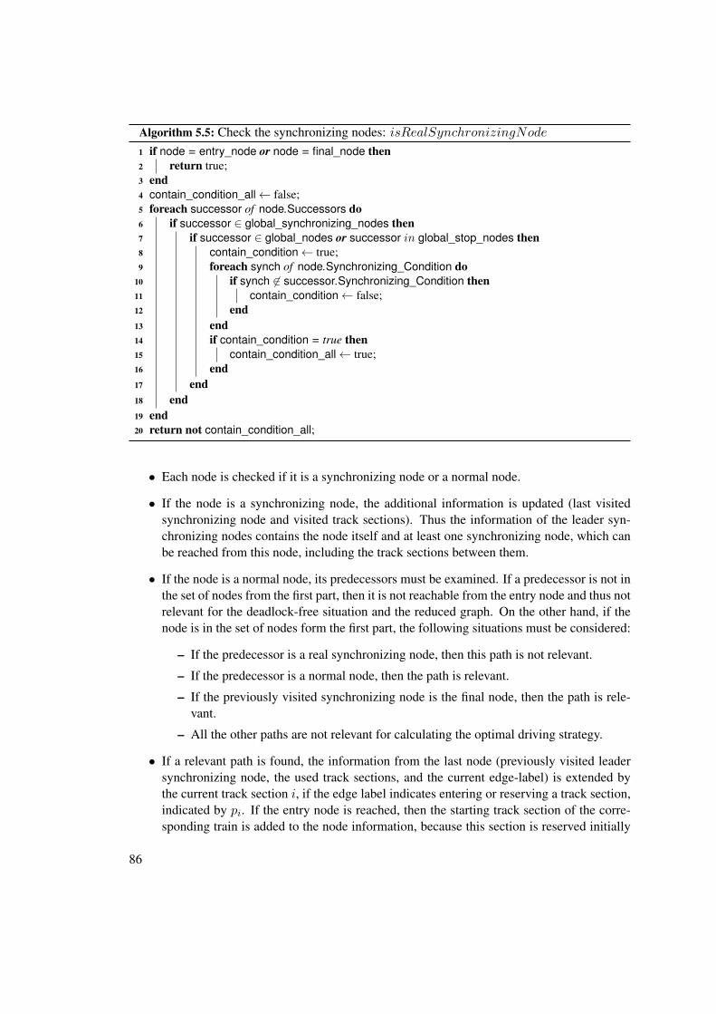
Algorithm 5.5: Check the synchronizing nodes: isRealSynchronizingNode1 if node = entry_node or node = final_node then2 return true;3 end4 contain_condition_all← false;5 foreach successor of node.Successors do6 if successor ∈ global_synchronizing_nodes then7 if successor ∈ global_nodes or successor in global_stop_nodes then8 contain_condition← true;9 foreach synch of node.Synchronizing_Condition do
10 if synch 6∈ successor.Synchronizing_Condition then11 contain_condition← false;12 end13 end14 if contain_condition = true then15 contain_condition_all← true;16 end17 end18 end19 end20 return not contain_condition_all;
• Each node is checked if it is a synchronizing node or a normal node.
• If the node is a synchronizing node, the additional information is updated (last visitedsynchronizing node and visited track sections). Thus the information of the leader syn-chronizing nodes contains the node itself and at least one synchronizing node, which canbe reached from this node, including the track sections between them.
• If the node is a normal node, its predecessors must be examined. If a predecessor is not inthe set of nodes from the first part, then it is not reachable from the entry node and thus notrelevant for the deadlock-free situation and the reduced graph. On the other hand, if thenode is in the set of nodes form the first part, the following situations must be considered:
– If the predecessor is a real synchronizing node, then this path is not relevant.
– If the predecessor is a normal node, then the path is relevant.
– If the previously visited synchronizing node is the final node, then the path is rele-vant.
– All the other paths are not relevant for calculating the optimal driving strategy.
• If a relevant path is found, the information from the last node (previously visited leadersynchronizing node, the used track sections, and the current edge-label) is extended bythe current track section i, if the edge label indicates entering or reserving a track section,indicated by pi. If the entry node is reached, then the starting track section of the corre-sponding train is added to the node information, because this section is reserved initially
86

and thus has no p-operation in the graph. Finally, the node itself and its node informationare added to the queue.
79542/1/18000
3->1:1/1000/5000
102413->1:1/1000/5000
T1: T2: T3:
805322/1/18000
T1: 1,2,5,6T2: T3:
206731/1/1000
T1: 1T2: T3:
828192->1:7/14000/18000
T1: T2: T3:
1
530611->2:2/5000/9000
2/1/1000
T1: 1,2,5T2: 1T3:
162091/1/1000
2->1:2/5000/9000
T1: 1T2: 1,2,3
T3:
36182->1:1/1000/5000
3/2/18000
T1: T2: 1,2T3: 7
312661->2:1/1000/5000
3/2/18000
T1: 1,2T2:
T3: 7
16092/1/1000
T1: T2: 1
T3: 7,4
108251/1/1000
T1: 1T2:
T3: 7,4
8653/2/1000
T1: T2:
T3: 7,4,2,1
887241/1/18000
T1: 6,7T2: 2,3
T3:
795082/1/18000
T1: 6T2: 2,3,7
T3:
1048971->3:7/14000/18000
2/1/1000
T1: 6,7T2: T3:
531901->2:2/5000/9000
3/2/180002/1/1000
T1: T2: T3: 7
580131->3:2/5000/90002->3:2/5000/9000
3->2:7/14000/18000
T1: T2: 2,3T3: 7,4
741872/1/1000
3->1:7/14000/18000
T1: 6T2:
T3: 7,4
T1: 2,5,6,7T2: T3:
T1: 2,5,6T2: 7T3:
163381/1/1000
2->1:2/5000/90003/2/18000
T1: T2: T3: 7
196491/1/1000
2->3:7/14000/18000
T1: T2: 7T3:
38812->1:1/1000/5000
T1: T2: T3: 4
T1: 1T2: 3T3:
T1: 5T2: 1T3:
315291->2:1/1000/5000
T1: T2:
T3: 4
T1: T2: 2T3:
T1: 2T2: T3:
10253->2:1/1000/50003->1:1/1000/5000
T1: T2: T3:
T1: T2: 3,7T3: 2,1
172331/1/1000
2->1:2/5000/9000
T1: 1T2: 3
T3: 2,1
100813/2/1000
T1: T2: 3,7T3: 2,1
166011/1/1000
2->3:2/5000/90003->2:7/14000/180002->1:2/5000/9000
T1: 1T2: 3T3:
T1: 2,5,6T2: 7T3:
T1: T2: 7T3:
897481/1/18000
T1: 2,5,6,7T2: T3:
T1: T2: T3:
200411/1/1000
T1: T2: 7T3:
476771/1/12000
3->2:7/14000/18000
T1: 2,5T2: T3:
1094571->3:7/14000/180001->2:7/14000/18000
T1: T2: T3:
817952->3:7/14000/180002->1:7/14000/18000
T1: T2: T3:
T1: T2: 2,3
T3:
1052892/1/1000
T1: T2:
T3: 7,4
784843/2/18000
T1: 6T2: 2,3
T3:
533261->2:2/5000/9000
2/1/1000
T1: T2: T3: 4
591661->3:2/5000/9000
2/1/18000
T1: T2: 7T3:
787472->3:2/5000/9000
3->2:7/14000/180003->1:7/14000/18000
T1: 6T2: T3:
T1: T2: 2,3
T3:
T1: 7T2: T3:
437491/1/120002/1/1000
540851->2:2/5000/9000
2/1/1000
T1: T2: T3:
T1: 6T2: 2,3,7
T3:
T1: 6,7T2: 2,3
T3:
1059212/1/1000
T1: 6,7T2: T3:
T1: 5T2: 1
T3: 2,1
839721/1/18000
3->2:1/1000/5000
T1: 5,6,7T2:
T3: 2,1
431171/1/120002/1/1000
T1: 5T2: 1T3:
1045453/2/1000
T1: 5,6,7T2:
T3: 2,1
T1: T2: 1,2,3
T3:
1047053->2:1/1000/5000
T1: T2: T3:
534531->3:2/5000/90001->2:2/5000/9000
2/1/1000
T1: T2: T3:
T1: T2: T3:
T1: T2: 2,3
T3:
T1: 6T2: T3:
T1: 6T2:
T3: 2,1
614531->3:2/5000/9000
T1: T2: T3:
T1: T2: 7
T3: 2,1
821872->1:7/14000/180003->1:7/14000/18000
T1: T2: 7T3:
891161/1/18000
2->3:2/5000/9000
T1: 7T2: T3:
T1: 2,5,6T2: T3:
164741/1/1000
2->1:2/5000/9000
T1: T2: T3: 4
T1: T2:
T3: 7,4
507251/1/12000
2->3:7/14000/18000
T1: 2,5T2: T3:
22412/1/1000
45132->1:1/1000/5000
T1: T2: 2T3:
T1: T2: 3,7
T3:
T1: 1T2: 3T3:
T1: T2:
T3: 4
114571/1/1000
321611->2:1/1000/5000
T1: 2T2: T3:
T1: 5T2: 1T3:
T1: 5,6,7T2: T3:
517491/1/12000
T1: 2,5T2: T3:
T1: 6T2: T3:
921641/1/18000
1128971->3:7/14000/180002->3:7/14000/18000
T1: T2: T3:
1130263/2/18000
T1: T2:
T3: 7
511171/1/12000
T1: 2,5T2: T3:
T1: T2: T3:
T1: T2: 7T3:
826592->1:7/14000/18000
3/2/1000
1137613/2/1000
T1: 7T2: T3:
T1: T2: T3:
113921
T1: T2: T3:
931881/1/18000
T1: 7T2: T3:
T1: T2:
T3: 4,2,1
1104811->2:7/14000/18000
T1: T2: T3:
1116342/1/18000
T1: T2: 7T3:
T1: 7T2: T3:
819243/2/18000
T1: T2: T3: 7
T1: T2:
T3: 4
T1: T2:
T3: 2,1
1106102/1/18000
T1: T2: T3:
1103211->2:7/14000/18000
3/2/1000
T1: T2: 7T3:
T1: T2: T3:
T1: T2: T3:
T1: T2: 7T3:
1095863/2/18000
T1: T2:
T3: 7
1098492->3:2/5000/9000
3->2:7/14000/180001->2:7/14000/18000
T1: T2: 2,3
T3:
T1: T2: T3: 4
T1: T2: T3:
T1: T2: 1T3:
T1: T2: 2,3
T3:
T1: T2:
T3: 2,1
T1: T2: T3:
T1: 6T2: T3:
T1: 6T2: T3:
T1: T2:
T3: 7,4
T1: T2: 1T3:
T1: 1T2: T3:
T1: T2: T3:
T1: T2:
T3: 2,1
T1: T2: T3:
T1: T2: T3:
Figure 5.9: Resulting graph (Part IV)
87
When the resulting graph is created, it contains only the entry node, the leader synchronizingnodes, and the final node. Algorithm 5.6 shows the functionality of the fourth part of the graphreduction algorithm.
The reduced graph of the example is illustrated in Figure 5.9 and contains 70 nodes (49 stopnodes, 40 synchronizing nodes, 21 synchronizing/stop nodes, start node and final node). Nodesare labeled with their node-id and the synchronization conditions. Edges are labeled by the usedtrack sections between two nodes.
Example 5.3. Node 109849 in Figure 5.9 is a multi-synchronizing node with the followingsynchronization conditions:
• 2 → 3 : 2. Additionally, the start position and the final position of track section 2 aregiven:
– Track section 2 starts at position 5 000 m for train T2.
– Track section 2 ends at position 9 000 m for train T2.
– Train T3 is driving in the opposite direction and thus, the start and end position ofthe track section are inverted.
• 3→ 2 : 7 with boundaries of track section 7: 14 000 m and 18 000 m.
• 1→ 2 : 7 with the same boundaries of the track section as before.
Example 5.4. Node 89116 in Figure 5.9 is a stop-node for train T1 and a synchronizing node,too:
• 1/1/18000 indicates that train T1 has a stop at position 18 000 m which is the end of itsjourney.
• Additionally, there is a synchronization at track section 2 between train T2 and T3.
Example 5.5. The label between node 74187 and 78747 contains the following:
• T1 :. No track section is passed by train T1 between these two nodes of the graph.
• T2 : 2, 3. Train T2 passes track section 2 and 3.
• T3 :. No track section is passed by train T3.
Due to the reduction algorithm, only synchronizing nodes remain in the graph. For a betterreadability, the remaining nodes are not filled in Figure 5.9 as defined in Section 4.5.
88
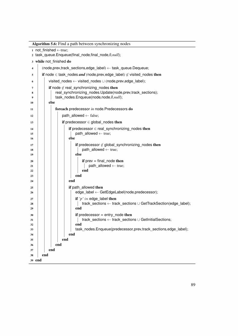
Algorithm 5.6: Find a path between synchronizing nodes1 not_finished←true;2 task_queue.Enqueue(final_node,final_node,∅,null);
3 while not_finished do
4 (node,prev,track_sections,edge_label)← task_queue.Dequeue;
5 if node ∈ task_nodes and (node,prev,edge_label) 6∈ visited_nodes then
6 visited_nodes← visited_nodes ∪ (node,prev,edge_label);
7 if node 6∈ real_synchronizing_nodes then8 real_synchronizing_nodes.Update(node,prev,track_sections);9 task_nodes.Enqueue(node,node,∅,null);
10 else
11 foreach predecessor in node.Predecessors do
12 path_allowed← false;
13 if predecessor ∈ global_nodes then
14 if predecessor ∈ real_synchronizing_nodes then15 path_allowed← true;16 else
17 if predecessor 6∈ global_synchronizing_nodes then18 path_allowed← true;19 else
20 if prev = final_node then21 path_allowed← true;22 end23 end24 end
25 if path_allowed then26 edge_label← GetEdgeLabel(node,predecessor);
27 if ’p’ in edge_label then28 track_sections← track_sections ∪ GetTrackSection(edge_label);29 end
30 if predecessor = entry_node then31 track_sections← track_sections ∪ GetInitialSections;32 end33 task_nodes.Enqueue(predecessor,prev,track_sections,edge_label);34 end35 end36 end37 end38 end39 end
89
5.3 Determine all possible routes
After the graph is reduced as described in Section 5.2, it remains to calculate all possible routesfor each train. If trains have more than one possible route on their journey there exists severalcombinations of the routes:
R =
n∏i=0
ri (5.2)
where R is the number of combinations, n is the number of trains, and ri is the number ofroutes for train i. There may exist some combinations which lead to deadlock situations. Thesecombinations of routes must not be considered for the overall result. In the previous sectionthe graph was created, deadlocks were eliminated, and the graph was reduced to the relevantnodes. So the resulting graph is the basis for further calculations without deadlocks. To find allpossible combinations of the routes of all trains within the railway system, the reduced graphis traversed top-down, using a depth-first search algorithm. When the final node is reached, aroute is found and the passed track sections of each train are added to a set of routes. Each routecontains at least the entry node and the final node. Between these two nodes, there might be stopnodes, if the train has stops at railway stations or synchronizing nodes, if there is the demand ofa synchronization on track sections between trains.
Due to the result of the application of Kronecker Algebra, there might be several pathsbetween two synchronizing nodes with the same track sections. To ensure that each synchro-nization is done, all synchronizing and stop nodes, which are found while traversing the graphmust be saved in a set for a particular route. Each combination of routes has its own set with aunique id, which is created by the track sections of the involved routes.
Assume that there is a railway system, including two trains Tn and Tm and the track sectionsa, b, c, and d. Each train can use two routes to reach their destination:
• Tn: a→ b→ d and a→ c→ d
• Tm: d→ b→ a and d→ c→ a
Based on equation 5.2, there exist four combinations of the routes.
• a→ b→ d and d→ b→ a
• a→ b→ d and d→ c→ a
• a→ c→ d and d→ b→ a
• a→ c→ d and d→ c→ a
Obviously, the first and the fourth item above will result in a deadlock and thus only thesecond and third train will be available for the calculation of the optimal driving strategies.
90
5.4 Finding the optimal driving strategy
In the previous section all possible routes were determined. The last step of the algorithm con-sists of finding the optimal solution in terms of energy. It is necessary to calculate the energyconsumption for each route. A route might be partitioned into sub-tracks by stop nodes. Twotypes of sub-tracks can be distinguished:
• Sub-tracks without synchronization
• Sub-tracks with synchronization
Sub-tracks without synchronization
A sub-track of a particular route of a train does not contain the demand of a synchronizationif there exists no synchronization node between two stop nodes. As a result the train can driveundisturbed along its route and its driving strategy can be calculated as described in Chapter 3(single trip optimization).
Sub-tracks with synchronization
If there exists at least one synchronization node within a sub-track, the calculation of the optimaldriving strategy is more complex than the single trip optimization. The following restrictionswill be used in this chapter:
• Trains are denoted by T and a particular train j by T j .
• In general, travel time values are denoted by t and for a particular train j by tj . If thetime value is related to a track section i, a subscript is used: ti and tji for train j on tracksection i, respectively. To indicate the minimum travel time an underline is used, e.g. theminimum travel time for train j on track section i is denoted by tji . For the maximumtravel time an overline is used, e.g. the maximum travel time for train j on track section iis denoted by tji .
• In general, the entering of track sections (e.g. section i) is denoted by→ i (as subscript)and the leaving of section i by i →, respectively.
By using the notions above, the following definitions for trains are given:
Definition 5.2 (Leaving trains). A train j, which is about to leave track section i is denoted byT j
i→.
Definition 5.3 (Entering trains). A train k, which is about to enter a track section i is denotedby T k
→ i .
In addition, some instants of time, which are used in the synchronization between trains mustbe defined:
91
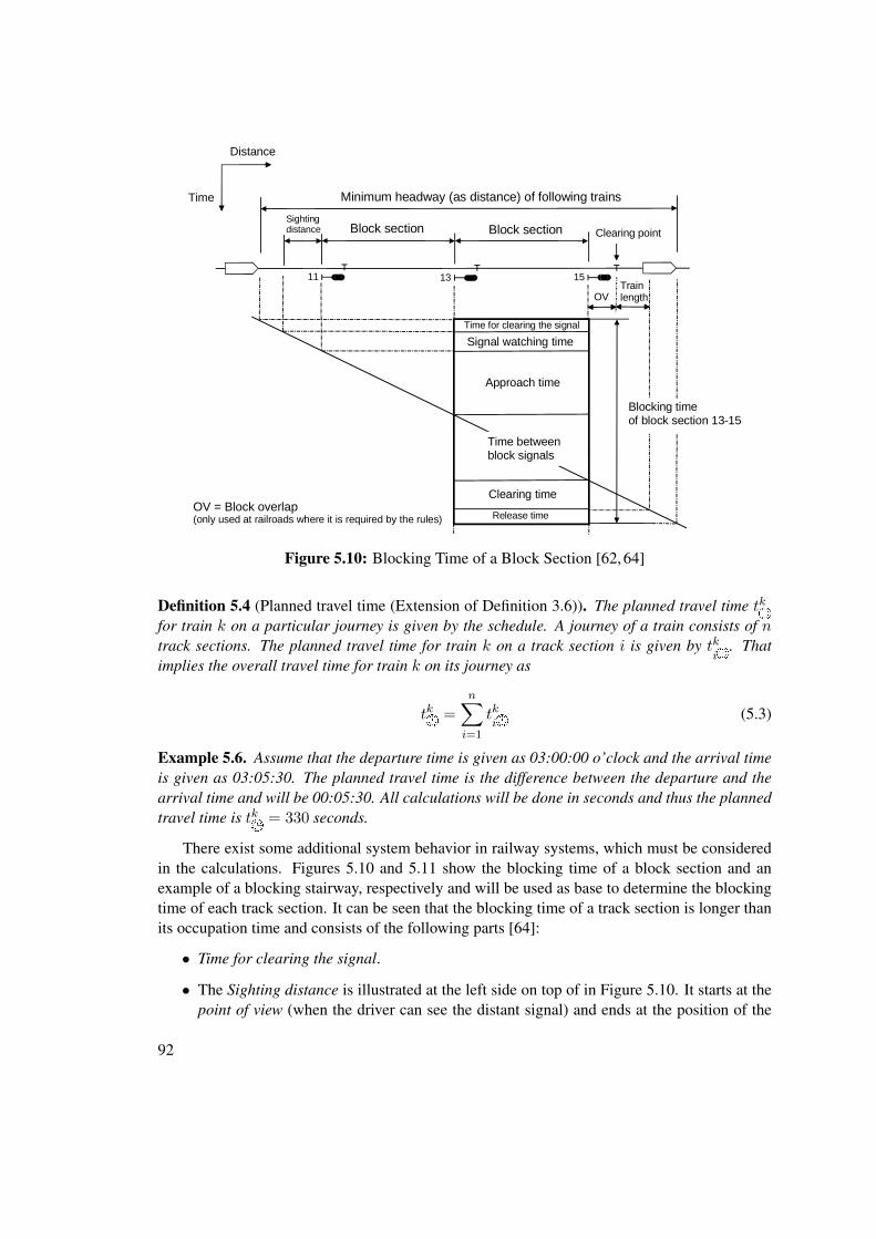
Block section
11 13
Clearing point
Minimum headway (as distance) of following trains
Trainlength
Sightingdistance
Blocking timeof block section 13-15
Approach time
Signal watching time
Time for clearing the signal
Clearing time
Release time
Time betweenblock signals
15
Block section
Time
Distance
OV
OV = Block overlap(only used at railroads where it is required by the rules)
Figure 5.10: Blocking Time of a Block Section [62, 64]
Definition 5.4 (Planned travel time (Extension of Definition 3.6)). The planned travel time tk�
for train k on a particular journey is given by the schedule. A journey of a train consists of ntrack sections. The planned travel time for train k on a track section i is given by tk
i�. That
implies the overall travel time for train k on its journey as
tk�
=n∑
i=1
tki�
(5.3)
Example 5.6. Assume that the departure time is given as 03:00:00 o’clock and the arrival timeis given as 03:05:30. The planned travel time is the difference between the departure and thearrival time and will be 00:05:30. All calculations will be done in seconds and thus the plannedtravel time is tk
�= 330 seconds.
There exist some additional system behavior in railway systems, which must be consideredin the calculations. Figures 5.10 and 5.11 show the blocking time of a block section and anexample of a blocking stairway, respectively and will be used as base to determine the blockingtime of each track section. It can be seen that the blocking time of a track section is longer thanits occupation time and consists of the following parts [64]:
• Time for clearing the signal.
• The Sighting distance is illustrated at the left side on top of in Figure 5.10. It starts at thepoint of view (when the driver can see the distant signal) and ends at the position of the
92

Time
Distance
Figure 5.11: Blocking Time Stairway [62, 64]
distant signal. The time from seeing the signal until the train passes it, is called Signalwatching time.
• The Approach Time gives the complete time while the train is between the distant signaland the beginning of the section.
• The time while the train is within the track section is called Time between block signals.
• The time between leaving a track section and completely passing a clearing point (e.g. allaxis passed an axle counter) is called Clearing time.
• In the end an additional offset is needed for releasing the track section (Release time).
As a result a track section will be blocked some given time for clearing the signal before thetrain arrives the point of view and released some additional release time after the complete trainhas passed the clearing point (e.g. an axle counter). The following definitions are based on theseassumptions and will be used for synchronization of trains using a common track section.
Definition 5.5 (Blocking and releasing a track section). A track section i is blocked by a train kat tk→ i and released at tki→. It follows that the complete blocking time tki of a track section i by
train k istki = tki→ − t
k→ i (5.4)
Definition 5.6 (Earliest release time). The earliest instant of time for train j to release a tracksection i is denoted by tji→. This value is calculated in accordance to the schedule and indicates
93
the earliest instant of time when a train releases a track section, assuming that it arrives at itsdestination within the planned travel time.
Definition 5.7 (Latest release time). The latest instant of time for train j to release a tracksection i is denoted by tji→. This value is calculated in accordance to the schedule and indicatesthe latest instant of time when a train releases a track section, assuming that it arrives at itsdestination within the planned travel time.
Definition 5.8 (Earliest reservation time). The earliest instant of time for train k to reserve atrack section i is denoted by tk
→ i . This value is calculated in accordance to the schedule andindicates the earliest instant of time when a train reserves a track section, assuming that itarrives at its destination within the planned travel time.
Definition 5.9 (Latest reservation time). The latest instant of time for train k to reserve a tracksection i is denoted by tk→ i . This values is calculated in accordance to the schedule and indicatesthe latest instant of time when a train reserves a track section, assuming that it arrives at itsdestination within the planned travel time.
In contrast to the release and reservation time values which are calculated at the point ofview or at the axle counter, regarding the time for clearing the signal and the release time, thefollowing definition for the input and output speed values, which are needed for the calculationof the driving strategy, are defined at the beginning and the end of a track section, respectively.
Definition 5.10 (Output speed (Extension of Definition 3.7)). The speed value of train j whenleaving track section i is called output speed, denoted by vij→. The highest and lowest output
speed values of train j when leaving a track section i while satisfying the schedule are vij→ and
vij→, respectively.
Definition 5.11 (Input speed (Extension of Definition 3.8)). The speed value of train j whenentering track section i is called input speed, denoted by vi
→ j . The highest and lowest input
speed values of train j when entering a track section i while satisfying the schedule are denotedby vi
→ j and vi→ j , respectively.
Obviously, vj→ i = vji-1→ for all 1 < i ≤ n, where n is the number of track sections4. The
first track section of a track or sub-track, starting at a railway station has an input speed valueof 0 km/h and the last section of a journey, ending at a station has an output speed of 0 km/h.If the calculation starts while the train is driving along its journey, its current speed is used asinput parameter of the calculation.
Definition 5.12 (Track section start and end position). A track section is bounded by its startposition s|i and its end position si|.
4Track section i is the successor of section i− 1 on the route.
94

Based on the definitions 5.5–5.9, the following equations must be valid to ensure that thetrain will arrive at its destination in time:
tji→ ≤ tj
i→ ≤ tj
i→ (5.5)
tk→ i ≤ t
k
→ i ≤ tk
→ i (5.6)
Synchronizing of trains
As already mentioned, trains must be synchronized if they want to use the same track section.In particular, a train can enter a track section only if it was already released by the other train.
Example 5.7. Assume that there are two trains, namely Tj and Tk, which want to use tracksection i. Based on the schedule the time values (in seconds) in Table 5.4 are calculated.
Tj Tk Tk′
tj→ i = 100 tk
→ i = 400 tk′
→ i = 320
tj
→ i = 150 tk
→ i = 450 tk′
→ i = 330
tji→ = 300 tki→ = 600 tk′
i→ = 520
tj
i→ = 350 tk
i→ = 650 tk′
i→ = 530
Table 5.4: Time values for synchronization
Track section i is blocked by train Tj in the worst case from 100 s to 350 s. As train Tk willenter track section i at the earliest after 400 s, no synchronization is needed between these twotrains. Now, assume train Tk′ is used instead of Tk. Now, there is an overlap between the twoinstants of time of train Tj for leaving the section and Tk′ entering the track section. As a resultTj must have left track section i at the latest after 330 s. Otherwise train Tk′ will not be in timeat its destination.
The algorithm is designed to find all solutions where all conflicts are avoided and the trainsarrive at their destination within the planned travel time. Now assume that train Tk wants to entera track section, which is blocked by Tj . Based on these assumptions the following equation mustbe valid for Tk
tk→ i > tji→ (5.7)
and on the other hand for Tjtj
i→ < tk
→ i (5.8)
The set S contains all trains which are part of the synchronization. Based on the aboverestrictions, the previously defined instants of time must be slightly modified:
tk∗→ i = max
j∈S, j 6=k
(tk→ i , t
j
i→
)(5.9)
tj∗i→ = max
j∈S, j 6=k
(tk
→ i , tj
i→
)(5.10)
95
tk
→ i and tji→ remain unchanged:
tk∗→ i = t
k
→ i (5.11)
tj∗i→ = tji→ (5.12)
For each synchronization between train j and k on track section i, these four time values(tk∗→ i , tk∗→ i , tj∗i→, tj∗i→) are relevant. Only solutions where no overlap between the instants of
time for entering and leaving a track section are allowed to be taken into account for finding theoptimal solution in terms of minimal energy consumption. Before analyzing the synchronizingnodes, these time values are computed for every pair of trains involved in a synchronizationcondition.
Analysis of synchronizing nodes
The next step is to analyze the synchronizing nodes of each route. Three types of routes can bedistinguished:
• No synchronization between trains is needed.
• No synchronization between trains is possible.
• Synchronization between trains is needed.
No synchronization needed. There are several situations where no synchronization betweentrains is needed:
• A track section is used by a single train.
• A track section i is used by more than one train, but there is no overlap of the blockingtime of a leaving train j and an entering train k, written as
tk∗→ i > t
j∗i→ (5.13)
If no synchronization is needed, the corresponding synchronization condition is removedfrom the synchronizing node. If all synchronization conditions are removed from a node, thenode itself is removed from the route. Due to the schedule it might be possible that all syn-chronizing nodes are removed from a route and thus, only the entry node and the final nodewill remain and the optimal driving strategy is calculated by the single trip optimization fromChapter 3.
No synchronization possible. A synchronization between two trains on a particular track sec-tion i is not possible if the following equation is valid:
tj∗i→ > tk∗→ i (5.14)
96
If a synchronization is not possible, then at least one train would not be able to reach its des-tination within the planned travel time. As the algorithm considers only results with a punctualarrival at each destination for the calculation of the driving strategies, the route is not taken intoaccount for the overall result.
Synchronization is needed. If the following conditions are valid, a synchronization on tracksection i between the leaving train j and the entering train k is possible and the node and itssynchronization condition will remain unchanged:
tk∗→ i ≤ t
k∗→ i (5.15)
tj∗i→ ≤ tj∗i→ (5.16)
tk∗→ i ≤ t
j∗i→ (5.17)
There are several situations, which may occur after the instants of time are calculated andtheir relations are analyzed:
• If all routes are removed, it is not possible that the trains will reach their destinations intime. Possible solutions are adaptation of the time table or reassignment of the routes (e.g.a train might use an alternative route).
• If all routes consist of the entry node and the final node only, there will be no influencebetween all trains within the railway network and thus the optimal driving strategy foreach train can be calculated independently from each other.
• For all routes consisting of at least one synchronizing node, the optimal driving strategyis calculated as described in the following section.
Determining the optimal driving strategy
Each node within the resulting routes must be analyzed. For this reason the nodes put in as-cending order by their node ids. As a result, the positions which are part of the synchronizationconditions are also ordered correctly. The stop nodes divide the complete complete track intosub-tracks. Due to the synchronization nodes, the sub-tracks are divided into several parts.
If a train is involved in a synchronization condition, the node, in particular the track sectionfrom the synchronization condition is relevant for the train. Based on the Definitions 5.6–5.11,the relevant time and speed values for the corresponding track section are calculated and savedin a vector together with the synchronization position. For a train entering a track section thestart position of the track is used as synchronization position and for a leaving train, the endposition is used, respectively. For each route and within the route for each train a separate vectoris used to save the data. This procedure is repeated for each node of the route until the final nodeis reached. If available, the next route is analyzed in the same way. If all routes and their nodesare analyzed, the optimal driving strategies can be calculated.
97
The determination of the optimal driving strategy is done for each route and in each routefor each train. So the calculation starts with the first train of the first route. Due to the fact thatthe complete track is split up into several parts and each part can have several output speed val-ues, in combination with several travel time values, a recursive algorithm will calculate severaldriving strategies for the overall result. The algorithm calculates the optimal driving strategybetween two positions, taken from the vector. The input speed of the current calculation is basedon the previous calculation, in other words, the input speed is the output speed of the previouscalculation. The output speed can vary between the minimum and maximum output speed value(see Definitions 5.10). The travel time is again based on the previous calculation and can varybetween the minimum and maximum travel time values (see Definition 5.6–5.9). The algorithmfrom Chapter 3 calculates the optimal driving strategy for the given input parameters. If a solu-tion is found, the calculated output values are taken as input parameters for the next part. Thisprocedure is repeated until the last element of the vector is reached. Then the calculation for thenext train within the system starts and when all computations of all trains are finished, the sameprocedure is done for the next route.
The instant of time for entering a track section is the sum of the travel time of each previouslypassed track section
∑i−1j=1 ∆tkj , the instant of time for leaving the section is bounded by tj∗i→
and tj∗i→. As a consequence, the following equation must be valid for the travel time on tracksection i:
tk∗i→ −i−1∑j=1
∆tkj ≤ tki ≤ tk∗i→ −
i−1∑j=1
∆tkj (5.18)
and thus
∆tki = tk∗i→ −i−1∑j=1
∆tkj (5.19)
∆tki = t
k∗i→ −
i−1∑j=1
∆tkj (5.20)
The travel time of a train k on track section i is bounded by ∆tki and ∆tki .
Assuming ∆tki = 180 s and ∆tki = 210 s, the best result in terms of energy consumption
may be between these two values. Due to restrictions on the calculation time, it might not bepossible or efficient to calculate the optimal driving strategy for each travel time value betweenthese values, e.g. for 180 s, 181 s, 182 s and so on. There exits an algorithm parameter to adjustthe time offset between two travel time values ∆t+ in seconds. Thus the algorithm will calculatethe optimal driving strategy for
∆tki ,∆tki + ∆t+,∆t
ki + 2 ·∆t+,∆tki + 3 ·∆t+ . . .∆tki .
As already mentioned, an input and output speed exists for each track section. The inputspeed is fixed, as it is equal to the output speed of the previous section (vj
→ i = vji-1→). To
98

find the optimal driving strategy, the output speed of each part of the track may be between theminimum and maximum output speed value. Thus the algorithm will use several speed valuesbetween these borders. The step size of these speed values can be adjusted by the algorithmparameter ∆v+ in km/h. As a result, the output speed for the calculation of the driving strategyfor train j on track section i is
vij→, vi
j→ + ∆v+, vi
j→ + 2 ·∆v+, vij→ + 3 ·∆v+ . . . vij→.
To sum up the functionality of the algorithm, the calculation of the overall result works asfollows:
• Start at the first route.
– Start at the first train with the following recursive algorithm.
∗ Start at the first part of the track with a given input speed (e.g. 0 km/h, whenstarting at a railway station).
∗ Calculate the driving strategies for all combinations of possible travel times andoutput speed values and use the calculated values as input for the next part.
∗ Repeat until the last position of the route is reached.
– Repeat until the driving strategies for all trains have been calculated.
• Repeat until all routes have been analyzed.
Thus, the algorithm calculates various driving strategies for each train. The last step ofthe optimization algorithm is to find the best solution in terms of energy consumption. Forthis reason all combinations of the results of the involved trains must be analyzed. As thereare several instants of time for entering and leaving a track section, an overlap between a trainentering and another one leaving a track section may occur. Such results are not valid and mustbe discarded from the set of results. Consequently, the results must be checked, if they fulfill thefollowing restrictions:
• Each train is within its schedule.
• A track section can be used only if it is not occupied by another train. In other words, traink can enter a track section i only, after it was released by another train j: tk∗
→ i ≥ tj∗i→ foreach track section i, where train j and k are involved in the synchronization.
• E → min, where E is the complete energy consumption of all trains.
The algorithm to determine the optimal driving strategy is designed to run on multi-coreCPUs. The calculation of the energy demand for each driving strategy (with different travel timeand output speed values) can be easily parallelized, as the calculations are independent fromeach other.
It can be easily seen, that the execution time of the algorithm grows exponentially in thenumber of track sections. However, the model behaves well for practical situations, e.g. a smallnumber of trains (two in almost all cases) and a small number of track sections or for systemswith less synchronizations between trains.
99
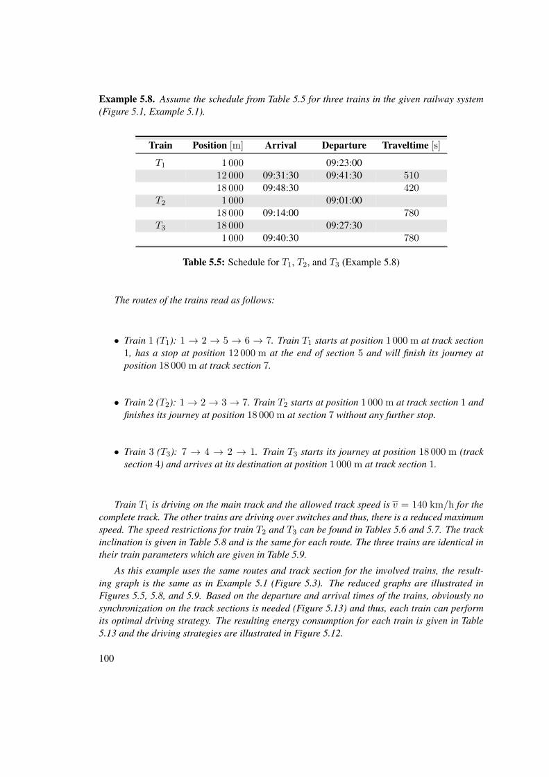
Example 5.8. Assume the schedule from Table 5.5 for three trains in the given railway system(Figure 5.1, Example 5.1).
Train Position [m] Arrival Departure Traveltime [s]
T1 1 000 09:23:0012 000 09:31:30 09:41:30 51018 000 09:48:30 420
T2 1 000 09:01:0018 000 09:14:00 780
T3 18 000 09:27:301 000 09:40:30 780
Table 5.5: Schedule for T1, T2, and T3 (Example 5.8)
The routes of the trains read as follows:
• Train 1 (T1): 1 → 2 → 5 → 6 → 7. Train T1 starts at position 1 000 m at track section1, has a stop at position 12 000 m at the end of section 5 and will finish its journey atposition 18 000 m at track section 7.
• Train 2 (T2): 1→ 2→ 3→ 7. Train T2 starts at position 1 000 m at track section 1 andfinishes its journey at position 18 000 m at section 7 without any further stop.
• Train 3 (T3): 7 → 4 → 2 → 1. Train T3 starts its journey at position 18 000 m (tracksection 4) and arrives at its destination at position 1 000 m at track section 1.
Train T1 is driving on the main track and the allowed track speed is v = 140 km/h for thecomplete track. The other trains are driving over switches and thus, there is a reduced maximumspeed. The speed restrictions for train T2 and T3 can be found in Tables 5.6 and 5.7. The trackinclination is given in Table 5.8 and is the same for each route. The three trains are identical intheir train parameters which are given in Table 5.9.
As this example uses the same routes and track section for the involved trains, the result-ing graph is the same as in Example 5.1 (Figure 5.3). The reduced graphs are illustrated inFigures 5.5, 5.8, and 5.9. Based on the departure and arrival times of the trains, obviously nosynchronization on the track sections is needed (Figure 5.13) and thus, each train can performits optimal driving strategy. The resulting energy consumption for each train is given in Table5.13 and the driving strategies are illustrated in Figure 5.12.
100
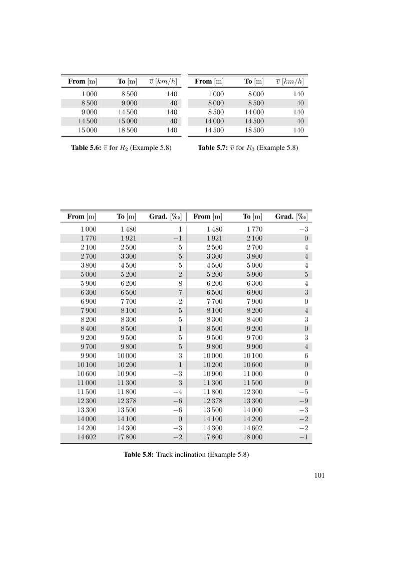
From [m] To [m] v [km/h]
1 000 8 500 1408 500 9 000 409 000 14 500 140
14 500 15 000 4015 000 18 500 140
Table 5.6: v for R2 (Example 5.8)
From [m] To [m] v [km/h]
1 000 8 000 1408 000 8 500 408 500 14 000 140
14 000 14 500 4014 500 18 500 140
Table 5.7: v for R3 (Example 5.8)
From [m] To [m] Grad. [h] From [m] To [m] Grad. [h]
1 000 1 480 1 1 480 1 770 −31 770 1 921 −1 1 921 2 100 02 100 2 500 5 2 500 2 700 42 700 3 300 5 3 300 3 800 43 800 4 500 5 4 500 5 000 45 000 5 200 2 5 200 5 900 55 900 6 200 8 6 200 6 300 46 300 6 500 7 6 500 6 900 36 900 7 700 2 7 700 7 900 07 900 8 100 5 8 100 8 200 48 200 8 300 5 8 300 8 400 38 400 8 500 1 8 500 9 200 09 200 9 500 5 9 500 9 700 39 700 9 800 5 9 800 9 900 49 900 10 000 3 10 000 10 100 6
10 100 10 200 1 10 200 10 600 010 600 10 900 −3 10 900 11 000 011 000 11 300 3 11 300 11 500 011 500 11 800 −4 11 800 12 300 −512 300 12 378 −6 12 378 13 300 −913 300 13 500 −6 13 500 14 000 −314 000 14 100 0 14 100 14 200 −214 200 14 300 −3 14 300 14 602 −214 602 17 800 −2 17 800 18 000 −1
Table 5.8: Track inclination (Example 5.8)
101
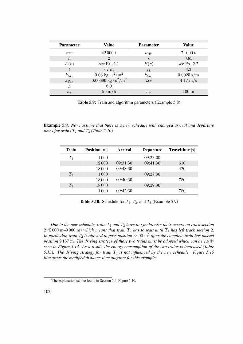
Parameter Value Parameter Value
mT 42 000 t mW 72 000 tn 2 r 0.85
F (v) see Ex. 2.1 B(v) see Ex. 2.2l 67 m fL 3.3
kSt1 0.03 kg · s2/m2 kSa1 0.0025 s/mkSa2 0.00696 kg · s2/m2 ∆v 4.17 m/sρ 6.0v+ 5 km/h s+ 100 m
Table 5.9: Train and algorithm parameters (Example 5.8)
Example 5.9. Now, assume that there is a new schedule with changed arrival and departuretimes for trains T2 and T3 (Table 5.10).
Train Position [m] Arrival Departure Traveltime [s]
T1 1 000 09:23:0012 000 09:31:30 09:41:30 51018 000 09:48:30 420
T2 1 000 09:27:3018 000 09:40:30 780
T3 18 000 09:29:301 000 09:42:30 780
Table 5.10: Schedule for T1, T2, and T3 (Example 5.9)
Due to the new schedule, train T1 and T2 have to synchronize their access on track section2 (5 000 m–9 000 m) which means that train T2 has to wait until T1 has left track section 2.In particular, train T2 is allowed to pass position 3 600 m5 after the complete train has passedposition 9 167 m. The driving strategy of these two trains must be adopted which can be easilyseen in Figure 5.14. As a result, the energy consumption of the two trains is increased (Table5.13). The driving strategy for train T3 is not influenced by the new schedule. Figure 5.15illustrates the modified distance-time diagram for this example.
5The explanation can be found in Section 5.4, Figure 5.10.
102

5 10 150
20
40
60
80
100
120
140
Position [km]
Spe
ed [k
m/h
]
5 10 150
20
40
60
80
100
120
140
Position [km]
Spe
ed [k
m/h
]
5 10 150
20
40
60
80
100
120
140
Position [km]
Spe
ed [k
m/h
]
Figure 5.12: Optimal driving strategy (Example 5.8)
5 10 15
09:10
09:20
09:30
09:40
Position [km]
Figure 5.13: Distance-Time diagram (Example 5.8)
103

5 10 150
20
40
60
80
100
120
140
Position [km]
Spe
ed [k
m/h
]
5 10 150
20
40
60
80
100
120
140
Position [km]
Spe
ed [k
m/h
]
5 10 150
20
40
60
80
100
120
140
Position [km]
Spe
ed [k
m/h
]
Figure 5.14: Optimal driving strategy (Example 5.9)
5 10 15
09:25
09:30
09:35
09:40
09:45
Position [km]
Figure 5.15: Distance-Time diagram (Example 5.9)
Example 5.10. This example, again, will use the same infrastructure. The schedule is modifiedas shown in Table 5.11.
104
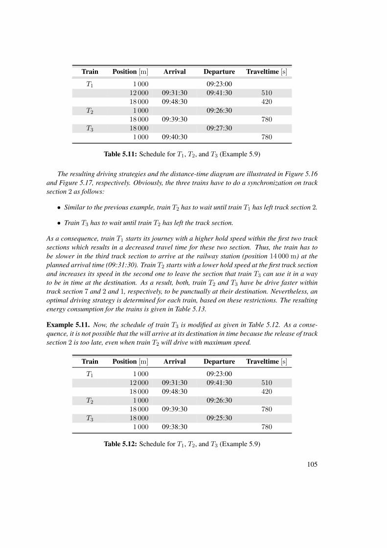
Train Position [m] Arrival Departure Traveltime [s]
T1 1 000 09:23:0012 000 09:31:30 09:41:30 51018 000 09:48:30 420
T2 1 000 09:26:3018 000 09:39:30 780
T3 18 000 09:27:301 000 09:40:30 780
Table 5.11: Schedule for T1, T2, and T3 (Example 5.9)
The resulting driving strategies and the distance-time diagram are illustrated in Figure 5.16and Figure 5.17, respectively. Obviously, the three trains have to do a synchronization on tracksection 2 as follows:
• Similar to the previous example, train T2 has to wait until train T1 has left track section 2.
• Train T3 has to wait until train T2 has left the track section.
As a consequence, train T1 starts its journey with a higher hold speed within the first two tracksections which results in a decreased travel time for these two section. Thus, the train has tobe slower in the third track section to arrive at the railway station (position 14 000 m) at theplanned arrival time (09:31:30). Train T2 starts with a lower hold speed at the first track sectionand increases its speed in the second one to leave the section that train T3 can use it in a wayto be in time at the destination. As a result, both, train T2 and T3 have be drive faster withintrack section 7 and 2 and 1, respectively, to be punctually at their destination. Nevertheless, anoptimal driving strategy is determined for each train, based on these restrictions. The resultingenergy consumption for the trains is given in Table 5.13.
Example 5.11. Now, the schedule of train T3 is modified as given in Table 5.12. As a conse-quence, it is not possible that the will arrive at its destination in time because the release of tracksection 2 is too late, even when train T2 will drive with maximum speed.
Train Position [m] Arrival Departure Traveltime [s]
T1 1 000 09:23:0012 000 09:31:30 09:41:30 51018 000 09:48:30 420
T2 1 000 09:26:3018 000 09:39:30 780
T3 18 000 09:25:301 000 09:38:30 780
Table 5.12: Schedule for T1, T2, and T3 (Example 5.9)
105
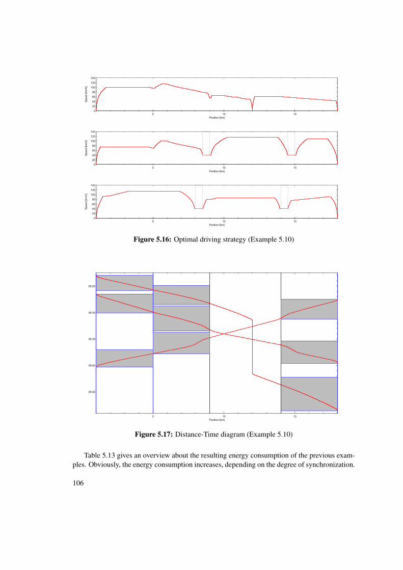
5 10 150
20
40
60
80
100
120
140
Position [km]
Spe
ed [k
m/h
]
5 10 150
20
40
60
80
100
120
140
Position [km]
Spe
ed [k
m/h
]
5 10 150
20
40
60
80
100
120
140
Position [km]
Spe
ed [k
m/h
]
Figure 5.16: Optimal driving strategy (Example 5.10)
5 10 15
09:25
09:30
09:35
09:40
09:45
Position [km]
Figure 5.17: Distance-Time diagram (Example 5.10)
Table 5.13 gives an overview about the resulting energy consumption of the previous exam-ples. Obviously, the energy consumption increases, depending on the degree of synchronization.
106
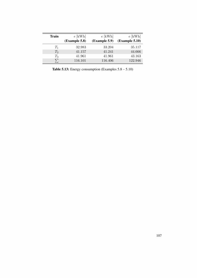
Train e [kWh](Example 5.8)
e [kWh](Example 5.9)
e [kWh](Example 5.10)
T1 32.983 33.204 35.117T2 41.157 41.241 44.666T3 41.961 41.961 43.163∑
116.101 116.406 122.946
Table 5.13: Energy consumption (Examples 5.8 – 5.10)
107

CHAPTER 6Extensions of the model
The presented model can act as base for further development in automation systems for railwaysystems. Some ideas for extending the model are introduced in this section.
6.1 Extension of the schedule
As already mentioned, the algorithm only calculates driving strategies for the trains, if they areall within the planned travel time. A possible extension could be to calculate driving strategiesfor unpunctual trains, too, assuming that the trains will be in time at another railway station. Inparticular, the schedule could be extended for intermediate stops to the end that the train can bein time at a defined final stop (cf. [39]).
Another approach to avoid conflicts on the track could be the modification of the departuretime of the trains. Therefore, the arrival time of the trains will be fixed, but the departure timecan be varied (e.g. the train must leave the railway station between 10:00:00 and 10:00:10). Thismay lead to a new driving strategy with less energy consumption because the train need notbreak and accelerate on the track, due to a blocked track section.
6.2 Train-priorities
The model can be extended by assigning priorities to trains. As a consequence, a train with ahigher priority may be handled in a different way than trains with low priority, e.g. when enteringtrack sections. The introduction of train-priorities may lead to unpunctuality for trains with lowpriority and thus the previous extension may be introduced together with the implementation oftrain-priorities.
109

6.3 Hard- and software-coupling
The algorithm may be coupled with some hardware parts and some dispatching or monitoringsoftware. The advantage would be that some important characteristics of the network can beconsidered in the calculations. In particular:
• The current schedule can be considered. It might be possible that the schedule may bechanged while operating due to delays, new train within the system or other factors thatmay have an influence on the dispatching.
• As the algorithm uses some track information (e.g. maximum allowed speed), it would bean advantage if this information can be updated online.
• If there is an energy bottleneck, some routes within the resulting graph may not be possibledue to a high energy demand. Such routes can be eliminated if the current state of thepower plants can be taken into account.
• Assume that the algorithm is implemented on a central computation unit and calculatesthe driving strategy for each train within the system. If the position of each train is knowexactly at each instant of time in the system, it can be compared with the calculated drivingstrategy. If there is a deviation between these two values, the algorithm must be restartedwith the new position (of each train). As a result, new driving strategies can be found fortrains within the system, depending on the influence of the deviant train.
6.4 Automated train control
Due to the fact that each train driver has a reaction time longer than the reaction time of anymachine, the best results can be achieved when the train control is done automatically, based onthe results of the algorithm. As a result, deviations and thus, new calculations can be avoided.
In general, each coupling to hardware or software modules can improve the correctness andthe performance of the algorithm and its results due to actuality of the used information.
110
CHAPTER 7Conclusion and prospect
This thesis is concerned with the development of an algorithm to determine the optimal drivingstrategy for each train within a railway network which is feasible in the field. Therefore thedependencies between the trains (e.g. for entering and leaving a track section) are analyzed andthe results are used in the calculations for the driving strategies. Due to the fact that there areseveral restrictions regarding the feasibility in the field, the calculated driving strategy is optimalunder these restrictions, but could theoretically be better. There exists a number of parametersto adjust the accuracy and the calculation time of the algorithm.
The algorithm is divided into two parts. The first one uses so-called Kronecker Algebrato determine all possible movements of the trains within the railway network. Conflicts (e.g.deadlocks or headway-conflicts) are found due to this mathematical model using matrices andoperations on them. Based on the results of these operations an optimal driving strategy is calcu-lated in the second part of the algorithm for each involved train under the assumption that eachtrain should arrive at its destination within the schedule and safety aspects are guaranteed. Thebest solution in terms of energy consumption is presented as overall result.
The algorithm uses an implementation of the train model and the track with a comprehensivenumber of adjustable parameters (e.g. train mass, number of wagons, various resistance values)to be near-term to reality. The better the mapping of the real world to the parameters the betterthe calculated result is.
As the algorithm is designed to determine only driving strategies where the trains will arriveat their destination in time, there might exist several situations (e.g. due to delays) where noresult is available. A useful extension of the algorithm might be to calculate driving strategiesfor unpunctual trains, too, as well as the usage of train priorities which could be considered inthe sequence of entering and leaving common used track sections.
111
As already mentioned in previous parts of this thesis, the algorithm is designed to run onmulti-core CPUs. As a result, the calculation time will decrease with a higher number of avail-able CPUs. Due to simplicity of the mathematical operations, the algorithm could be portedto graphic cards with a very high number of processing units which would result in a dramaticreduction of calculation time.
The development of the algorithm was part of the EcoRailNet project in the frame of theprogram New Energy 2020 (Project-ID: 834586). Several parts of the algorithm were tested inthe field with good results and valuable perceptions. Other parts were discussed within meetingsand presented on conferences and appear to be a good base for further development.
112
Bibliography
[1] Amie Albrecht, Phil Howlett, Peter Pudney, and Xuan Vu. Optimal train control: Analysisof a new local optimization principle. In American Control Conference (ACC), pages1928–1933, San Francisco, USA, Jun 2011.
[2] Thomas Albrecht. Energy-Efficient Train Operation. In Ingo A. Hansen, Jörn Pachl, andThomas Albrecht, editors, Railway, Timetable & Traffic: Analysis, Modelling, Simulation,pages 83–105. Eurailpress, 1 edition, 2008.
[3] Richard Bellman. Introduction to Matrix Analysis. Classics in Applied Mathematics.Society for Industrial and Applied Mathematics, 2nd edition, 1997.
[4] Jasna Blaškovic Zavada, Borna Abramovic, and Tomislav Cvek. Energy-efficient drive oftrains. In 22th International Symposium on Electronics in Transport ISEP 2014, Ljubljana,Sovenija, Mar 2014.
[5] Randall L. Brukardt. Ada 2012 Annotated Reference Manual, 2012.
[6] Olaf Brünger and Elias Dahlhaus. Running Time Estimation. In Ingo A. Hansen, JörnPachl, and Thomas Albrecht, editors, Railway, Timetable & Traffic: Analysis, Modelling,Simulation, pages 58–82. Eurailpress, Hamburg,Germany, 1 edition, 2008.
[7] Peter Buchholz and Peter Kemper. Efficient Computation and Representation of LargeReachability Sets for Composed Automata. Discrete Event Dyn. Systems, 12(3):265–286,2002.
[8] Ginautas Bureika, Rimantas Subacius, and Mika Kumara. Research on Energy Efficient ofRolling-Stock Operation. In The 6th International Scientific Conference “TRANSBALTICA2009”, pages 28–32, Apr 2009.
[9] Gabrio Caimi, Fabián A. Chudak, Martin Fuchsberger, Marco Laumanns, and Rico Zen-klusen. A new resource-constrained multicommodity flow model for conflict-free trainrouting and scheduling. Transportation Science, 45(2):212–227, May 2011.
[10] Gabrio Caimi, Martin Fuchsberger, Dan Burkolter, Thomas Herrmann, Raimond Wüst,and Samuel Roos. Conflict-free train scheduling in a compensation zone exploiting thespeed profile. In 3rd International Seminar on Railway Operations Modelling and Analysis(ISROR), Zürich, Switzerland, Feb 2009.
113

[11] Gabrio Caimi, Martin Fuchsberger, Marco Laumanns, and Marco Lüthi. A model pre-dictive control approach for discrete-time rescheduling in complex central railway stationareas. Computers & Operations Research, 39(11):2578–2593, 2012.
[12] Gabrio Caimi, Marco Laumanns, Kaspar Schüpbach, Stefan Wörner, and Martin Fuchs-berger. The periodic service intention as a conceptual frame for generating timetables withpartial periodicity. In Transportation Planning and Technology 34(4), pages 323–339,2011.
[13] Jiaxing Cheng, Yelena Davydova, Phil Howlett, and Peter Pudney. Optimal driving strate-gies for a train journey with non-zero track gradient and speed limits. IMA Journal ofMathematics Applied in Business & Industry, 10(0199921504):89–115, 1999.
[14] Rémy Chevrier, Grégory Marlière, Bogdan Vulturescu, and Joaquin Rodriguez. Multi-objective Evolutionary Algorithm for Speed Tuning Optimization with Energy Saving inRailway: Application and Case Study. In RailRome 2011, Rome, Italy, 2011.
[15] Colin Cole. Longitudinal Train Dynamics. In Simon Iwnicki, editor, Handbook of RailwayVehicle Dynamics, pages 239–278. Taylor & Francis Group, Boca Raton, USA, 2006.
[16] Yong Cui. Simulation-Based Hybrid Model for a Partially-Automatic Dispatching of Rail-way Operation. PhD thesis, Universität Stuttgart, 2010.
[17] Marc Davio. Kronecker Products and Shuffle Algebra. IEEE Trans. Computers, 30(2):116–125, 1981.
[18] Caroline Desprez and Housni Djellab. Traction energy saving by speed profile optimiza-tion. In Compendium of Papers for the Euro Working Group of Transportation, Paris,France, 2012.
[19] Edsger W. Dijkstra. Over Seinpalen. 1965.
[20] Edsger W. Dijkstra. Een algorithme ter voorkoming van de dodelijke omarming. n.d.
[21] Markus Ellinger. Energiesparende Fahrweise unter Berücksichtigung betrieblicher undtechnischer Parameter. Master thesis, Fachhochschule St. Pölten, 2013.
[22] Maria Pia Fanti, Alessandro Giua, and Carla. Seatzu. A deadlock prevention method forrailway networks using monitors for colored petri nets. In Systems, Man and Cybernetics,2003. IEEE International Conference on, volume 2, pages 1866–1873, Oct 2003.
[23] Rüdiger Franke, Markus Meyer, and Peter Terwiesch. Optimal Control of the Driving ofTrains. Automatisierungstechnik Methoden und Anwendungen der Steuerungs-, Regelungs-und Informationstechnik, 50(12):606–613, Dec 2002.
[24] Rüdiger Franke, Peter Terwiesch, and Markus Meyer. An algorithm for the optimal controlof the driving of trains. In Decision and Control, 2000. Proceedings of the 39th IEEEConference on, volume 3, pages 2123–2128, Dec 2000.
114
[25] Martin Fuchsberger. Solving the train scheduling problem in a main station area via aresource constrained space-time integer multi-commodity flow. Master thesis, ETH Zurich,2007.
[26] ÖBB-Produktion GmbH. Velocity-braking-force-diagram, 2014.
[27] ÖBB-Produktion GmbH. Velocity-traction-force-diagram, 2014.
[28] ÖBB-Produktion GmbH. Verzeichnis zulässiger Geschwindigkeiten, 2014.
[29] Iakov M. Golovitcher. Energy efficient control of rail vehicles. In Systems, Man, andCybernetics, 2001 IEEE International Conference on, volume 10, pages 658–663, Tuc-son,USA, 2001.
[30] Alexander Graham. Kronecker Products and Matrix Calculus with Applications. EllisHorwood Ltd., New York, USA, 1981.
[31] Peter Henderson and James H. Morris, Jr. A Lazy Evaluator. In 3rd ACM Symposium onPrinciples of Programming Languages, POPL ’76, pages 95–103, January 1976.
[32] Phil Howlett. Optimal strategies for the control of a train. Automatica, 32(4):519–532, Apr1996.
[33] Phil Howlett. The Optimal Control of a Train. Annals of Operations Research, 98(1-4):65–87, 2000.
[34] Phil Howlett and Peter Pudney. Energy-Efficient Train Control. Advances in IndustrialControl. Springer London, 1995.
[35] Phil Howlett, Peter Pudney, and Xuan Vu. Local energy minimization in optimal traincontrol. Automatica, 45(11):2692–2698, Sep 2009.
[36] Daniel Hürlimann. Opentrack railway technology. Website http://www.opentrack.at. Visited: 2014-11-25.
[37] Daniel Hürlimann. OpenTrack Manual, 2013.
[38] Wilfried Imrich, Sandi Klavzar, and Douglas F. Rall. Topics in Graph Theory: Graphs andTheir Cartesian Product. A K Peters Ltd, 2008.
[39] Jürgen Jacobs. Rescheduling. In Ingo A. Hansen, Jörn Pachl, and Thomas Albrecht,editors, Railway, Timetable & Traffic: Analysis, Modelling, Simulation, pages 182–191.Eurailpress, Hamburg,Germany, 1 edition, 2008.
[40] Birgit Jaekel and Thomas Albrecht. Interfacing conflict resolution and driver advisory sys-tems in railway operation. In Proceedings of the 3rd International Conference on Modelsand Technologies for Intelligent Transportation Systems (MT-ITS), pages 333–343, Dres-den, Germany, Dec 2013.
115

[41] Eugene Khmelnitsky. On an Optimal Control Problem of Train Operation. IEEE TRANS-ACTIONS ON AUTOMATIC CONTROL, 45(7):1257–1266, July 2000.
[42] Donald E. Knuth. The Art of Computer Programming, Volume 3: Sorting and Searching.Pearson Education, 1998.
[43] Donald E. Knuth. Combinatorial Algorithms, volume 4A of The Art of Computer Pro-gramming. Addison-Wesley, 2011.
[44] Werner Kuich and Arto K. Salomaa. Semirings, Automata, Languages. EATCS Mono-graphs on Theoretical Computer Science. Springer-Verlag GmbH, 1986.
[45] Gerhard Küster. On the Hurwitz Product of Formal Power Series and Automata. Theor.Comput. Sci., 83(2):261–273, 1991.
[46] D.H. Lee, Ian P. Milroy, and K. Tyler. Application of Pontryagin’s Maximum Principle tothe Semi-automatic Control of Rail Vehicles. In Proceedings of the Second Conference onControl Engineering, pages 233–236, Newcastle, Australia, 1982. Institution of EngineersAustralia.
[47] Liang Li, Wei Dong, Yindong Ji, and Zengke Zhang. A minimal-energy driving strategyfor high-speed electric train. Journal of Control Theory and Applications, 10(3):280–286,Aug 2012.
[48] Ulrich Linder. Optimierung von Fahrweisen im spurgeführten Verkehr und deren Umset-zung. PhD thesis, Technische Universität Berlin, 2004.
[49] Rongfang (Rachel) Liu and Iakov M. Golovitcher. Energy-efficient operation of rail vehi-cles. Transportation Research Part A: Policy and Practice, 37(10):917–932, Jul 2003.
[50] Quan Lu, Maged Dessouky, and Robert C. Leachman. Modeling train movements throughcomplex rail networks. ACM Trans. Model. Comput. Simul., 14(1):48–75, Jan 2004.
[51] Marco Lüthi. Evaluation of energy saving strategies in heavily used rail networks by im-plementing an integrated real-time rescheduling system. In Eduardo Pilo, editor, PowerSupply, Energy Management, and Catenary Problems, pages 75–86. WIT Press, 2010.
[52] Ullrich Martin. Verfahren zur Bewertung von Zug- und Rangierfahrten bei der Disposition.Schriftenreihe. Inst. für Eisenbahnwesen und Verkehrssicherung, 1995.
[53] Farhad Mehta, Farhad Rößiger, and Markus Montigel. Latent energy savings due to theinnovative use of advisory speeds to avoid occupation conflicts. In B. Ning and C.A Breb-bia, editors, Computers in Railways XII: Computer System Design and Operation in Rail-ways and Other Transit Systems (WIT Transactions on the Built Environment), volume 114,pages 99–108. WIT Press, 2010.
[54] Jeff Miller. Earliest Known Uses of Some of the Words of Mathematics, Rev. Aug. 1, 2011.Website: http://jeff560.tripod.com/k.html, 2012. Visited: 2014-11-25.
116

[55] Graham Mills and Peter J Pudney. The effects of deadlock avoidance on rail network ca-pacity and performance. In Proceedings of the 2003 mathematics-in-industry study group,pages 49–63. Australian Mathematical Society, 2008.
[56] Robert Mittermayr and Johann Blieberger. Shared Memory Concurrent System Verifica-tion using Kronecker Algebra. Technical report, Insitute of Computer-Aided Automation,TU Vienna, Austria, Vienna, Austria, Sep 2011.
[57] Robert Mittermayr and Johann Blieberger. Timing Analysis of Concurrent Programs.In Tullio Vardanega, editor, 12th International Workshop on Worst-Case ExecutionTime Analysis, volume 23 of OpenAccess Series in Informatics (OASIcs), pages 59–68,Dagstuhl, Germany, 2012. Schloss Dagstuhl–Leibniz-Zentrum fuer Informatik.
[58] Robert Mittermayr, Johann Blieberger, and Andreas Schöbel. Kronecker Algebra basedDeadlock Analysis for Railway Systems. PROMET-TRAFFIC & TRANSPORTATION,24(5):359–369, 2012.
[59] Masafumi Miyatake and Hideyoshi Ko. Optimization of train speed profile for mini-mum energy consumption. IEEJ Transactions on Electrical and Electronic Engineering,5(3):263–269, Apr 2010.
[60] Markus Montigel. Innovatives Bahnleitsystem optimiert den Zugverkehr im Lötschberg-Basistunnel. Signal + Draht, 6, 2008.
[61] Markus Montigel. Operations control system in the Lötschberg Base Tunnel. EuropeanRail Technology Review, 49:42–44, 2009.
[62] Joern Pachl and Thomas White. Analytical capacity management with blocking times. InTransportation Research Board. 83rd Annual Meeting, Jan 2004.
[63] Jörn Pachl. Steuerlogik für Zuglenkanlagen zum Einsatz unter stochastischen Betriebsbe-dingungen. PhD thesis, TU Braunschweig, 1993.
[64] Jörn Pachl. Timetable Design Principles. In Ingo A. Hansen, Jörn Pachl, and ThomasAlbrecht, editors, Railway, Timetable & Traffic: Analysis, Modelling, Simulation, pages9–42. Eurailpress, Hamburg,Germany, 1 edition, 2008.
[65] Jörn Pachl. Deadlock avoidance in railroad operations simulations. In Textfassung einesVortrages auf dem 90th Annual Meeting des Transportation Research Board in WashingtonDC, pages 23–27, 2011.
[66] E. Petersen and A Taylor. Line block prevention in rail line dispatch. In INFOR Journal,volume 21, pages 46–51, 1983.
[67] Brigitte Plateau. On the Stochastic Structure of Parallelism and Synchronization Modelsfor Distributed Algorithms. In ACM SIGMETRICS, volume 13, pages 147–154, 1985.
117

[68] Brigitte Plateau and Karim Atif. Stochastic Automata Network For Modeling ParallelSystems. IEEE Trans. Software Eng., 17(10):1093–1108, 1991.
[69] Alfons Radtke. Infrastructure Modelling. In Ingo A. Hansen, Jörn Pachl, and ThomasAlbrecht, editors, Railway, Timetable & Traffic: Analysis, Modelling, Simulation, pages43–57. Eurailpress, Hamburg,Germany, 1 edition, 2008.
[70] Xiaolu Rao, Markus Montigel, and Weidmann Ulrich. Railway capacity optimization byintegration of real-time rescheduling and automatic train operation. In IT13.RAIL, Zürich,Switzerland, 2013.
[71] Xiaolu Rao, Markus Montigel, and Ulrich Weidmann. Holistic optimization of train trafficby integration of automatic train operation with centralized train management. In C.A.Brebbia, N. Tomii, J.M. Mera, B Ning, and P. Tzieropoulos, editors, Computers in Rail-ways XIII: Computer System Design and Operation in the Railway and Other Transit Sys-tems (Wit Transactions on the Built Environment), volume 127, pages 39–50. WIT Press,2012.
[72] Andreas Schöbel, Bernhard Rüger, Andrew Nash, Jürgen Zajicek, Martin Turk, and Hart-mut Dannenberg. The potential for saving energy by more precisely calculating stationdwell times on commuter rail service. In 3rd International Seminar on Railway Opera-tions Modelling and Analysis: RailZurich2009 Conference, Zürich, Switzerland, 2009.
[73] Thomas Siefer. Simulation. In Ingo A. Hansen, Jörn Pachl, and Thomas Albrecht, editors,Railway, Timetable & Traffic: Analysis, Modelling, Simulation, pages 155–169. Eurail-press, Hamburg,Germany, 1 edition, 2008.
[74] N.S. Szabó and R.I. Tanaka. Residue arithmetic and its applications to computer technol-ogy. McGraw-Hill series in information processing and computers. McGraw-Hill, 1967.
[75] S. Tucker Taft, Pascal Leroy, Robert A. Duff, Randall L. Brukardt, and Erhard Ploedereder,editors. Ada 2005 Reference Manual. Springer-Verlag, 2006.
[76] Mark Volcic, Johann Blieberger, and Andreas Schöbel. Kronecker algebra and its broadapplications in railway systems. In EURO-ŽEL 2013: Recent Challenges for EuropeanRailways, pages 275–282, Žilina, Slovak Republic, June 2013.
[77] Mark Volcic, Johann Blieberger, and Andreas Schöbel. Kronecker algebra as a frame foroptimisation of railway operation. In 21st International Scientific Conference – TRANS-PORT 2013; Mechanics Transport Communications, volume 11/3, pages 57–63, Sofia,Bulgaria, October 2013.
[78] Mark Volcic, Johann Blieberger, and Andreas Schöbel. Kronecker algebra based modellingof railway operation. In Proceedings of the 3rd International Conference on Models andTechnologies for Intelligent Transportation Systems (MT-ITS), pages 345–356, Dresden,Germany, December 2013.
118
[79] Mark Volcic, Johann Blieberger, and Andreas Schöbel. Kronecker-Algebra und ihre breitgefächerten Anwendungen im Eisenbahnbereich. Signal + Draht, 7+8:15–18, 2014.
[80] Mark Volcic, Johann Blieberger, and Andreas Schöbel. Optimisation of railway operationby application of kronecker algebra. In CETRA 2014, pages 37–42, Split, Croatia, April2014.
[81] Mark Volcic, Johann Blieberger, and Andreas Schoebel. Kronecker Algebra based TravelTime Analysis for Railway Systems. In FORMS/FORMAT 2012 – 9th Symposium onFormal Methods for Automation and Safety in Railway and Automotive Systems, pages273–281, Braunschweig, Germany, Dec 2012.
[82] Xuan Vu. Analysis of necessary conditions for the optimal control of a train. PhD thesis,University of South Australia, Nov 2006.
[83] Michal Žarnay. Solving deadlock states in model of railway station operation usingcoloured petri nets. In Proceedings of Symposium FORMS/FORMAT - Formal Methodsfor Automation and Safety in Railway and Automotive Systems, pages 205–213, Budapest,Hungary, 2008.
[84] Yihui Wang, Bing Ning, Fang Cao, B. De Schutter, and T.J.J. van den Boom. A survey onoptimal trajectory planning for train operations. In Service Operations, Logistics, and In-formatics (SOLI), 2011 IEEE International Conference on, pages 589–594, Beijing,China,Jul 2011.
[85] Johann Georg Zehfuss. Ueber eine gewisse Determinante. Zeitschrift für Mathematik undPhysik, 3:298–301, 1858.
119


