Page 1
1
Energy Efficient Dynamic Resource
Optimization in NOMA System
Haijun Zhang,Senior Member, IEEE, Baobao Wang,
Chunxiao Jiang,Senior Member, IEEE, Keping Long,Senior Member, IEEE,
A. Nallanathan,Fellow, IEEE, Victor C. M. Leung,Fellow, IEEE, and
H. Vincent Poor,Fellow, IEEE
Abstract
Non-orthogonal multiple access (NOMA) with successive interference cancellation (SIC) is a
promising technique for next generation wireless communications. Using NOMA, more than one user
can access the same frequency-time resource simultaneously and multi-user signals can be separated
successfully using SIC. In this paper, resource allocationalgorithms for subchannel assignment and
power allocation for a downlink NOMA network are investigated. Different from the existing works,
here, energy efficient dynamic power allocation in NOMA networks is investigated. This problem is
explored using the Lyapunov optimization method by considering the constraints on minimum user
quality of service (QoS), the maximum transmit power limit.Based on the framework of Lyapunov
Haijun Zhang and Keping Long are with the Beijing Engineering and Technology Research Center for Convergence Networks
and Ubiquitous Services, University of Science and Technology Beijing, Beijing, 100083, China. (e-mail: [email protected] ,
[email protected] ).
Baobao Wang is with the College of Information Science and Technology, Beijing University of Chemical Technology, China
(e-mail: [email protected] ).
Chunxiao Jiang is with Tsinghua Space Center, Tsinghua University, Beijing 100084, P. R. China (e-mail:
[email protected] ).
A. Nallanathan is with the Queen Mary University of London, London, United Kingdom (Email: [email protected] ).
Victor C. M. Leung is with the Department of Electrical and Computer Engineering, The University of British Columbia,
Vancouver, BC, V6T 1Z4, Canada (e-mail: [email protected] ).
H. Vincent Poor is with the Department of Electrical Engineering, Princeton University, Princeton, NJ, USA (e-mail:
[email protected] ).
May 23, 2018 DRAFT
Page 2
2
optimization, the problem of energy efficient optimizationcan be broken down into three subproblems.
Two of which are linear and the rest can be solved by introducing Lagrangian function. The mathematical
analysis and simulation results confirm that the proposed scheme can achieve a significant utility
performance gain and the energy efficiency and delay tradeoff is derived as[O(1/V ),O(V )] with
V as a control parameter under maintaining the queue stability.
Index Terms
NOMA, Lyapunov optimization, power allocation, subchannel assignment
I. INTRODUCTION
In the past decade, orthogonal frequency division multipleaccess (OFDMA) has been widely
studied and has been adopted in 4th generation (4G) mobile communication systems [1], [2].
However, orthogonal channel access in OFDMA is becoming a limiting factor of spectrum
efficiency since each subchannel can only be used by at most one user in each time slot. With
the explosive growth of smart mobile devices and the increasing demands for higher spectral
efficiency, non-orthogonal multiple access (NOMA) has beenproposed to mitigate the consequent
heavy loading at the base station (BS) [3]–[5]. NOMA is a promising technique to realize
the massive connectivity in 5th generation (5G) mobile networks because NOMA can achieve
significant improvement in spectral efficiency with a lower receiver complexity by allowing
multiple users to share the same subchannel in the power domain [6]–[8].
The use of NOMA will result in inter-user interference sincemultiple users will share
the same resources [9]. Successive interference cancellation (SIC) can be applied at the end-
user receivers to mitigate this interference [10]. NOMA canachieve a capacity region that
significantly outperforms orthogonal multiple access schemes by power domain multiplexing
at the transmitter and SIC at the receivers [11]. The outage performance of NOMA was
evaluated in [12], while in [13], the authors investigated the system sum-rate of multiuser
NOMA single-carrier systems as well as proposing a suboptimal power allocation and presenting
a precoder design. Moreover, the authors addressed fairness considerations and posed a max-
min fairness problem for NOMA. In [15], an optimal power allocation strategy for the energy-
efficiency maximization of NOMA in single-carrier systems was investigated. The authors in
[16] investigated the subchannel assignment and power allocation using the difference of convex
May 23, 2018 DRAFT
Page 3
3
programming method. A suboptimal algorithm was proposed tosolve an uplink scheduling
problem with fixed transmission power for uplink NOMA in [17]and a greedy-based algorithm
was proposed to improve the throughput in uplink NOMA in [18]. In [19], a new spectrum
and energy efficient mmWave transmission scheme which integrates the concept of NOMA with
beamspace MIMO was proposed to break the fundamental limit.In [20], a hierarchical power
control solution to improve the spectrum and energy efficiency in NOMA-enabled vehicular
small cell networks was proposed by performing the joint optimization of cell association and
power control. In [21], a novel resource allocation design was investigated for NOMA enhanced
heterogeneous networks. However, the study of energy efficient subchannel assignment and
power allocation in multiple small cells with NOMA under theconstraints of minimum QoS
requirements and cross interference has not been well studied.
On contrary to the typically full buffer assumptions and snapshot-based models, delay is a
key metric to measure the QoS. The congestion performance for delay-tolerant services and the
stochastic and time-varying features of traffic arrivals should be considered in realistic wireless
networks. By utilizing Lyapunov optimization, which is an useful method for handling queue-
aware radio resource allocation problems, [22], [23] considered the impacts of stochastic traffic
arrivals and time-varying channel conditions on the systemperformance to stabilize the queues
of networks when optimizing performance metrics. In [22], the authors applied the framework of
Lyapunov optimization to balance the average throughput and average delay in energy efficient
OFDMA heterogeneous cloud networks. The authors in [23] adopted the Lyapunov optimization
framework in a two-tier OFDMA heterogeneous network under the hybrid access mode to
solve the dynamic optimization problem of resource allocation. In [24], an energy efficient
resource allocation algorithm was proposed to provide fairness among different small cell base
stations(SCBSs) based on the Nash bargaining solution. However, most of the existing works
considered resource allocation using Lyapunov optimization only in OFDMA systems. And to
the best of the authors’ knowledge, energy efficient resource allocation for time-varying NOMA
networks has not been well studied in the previous works.
In this paper, we investigate the subchannel and power allocation respectively in a multiple
downlink NOMA network by considering energy efficiency, quality of service (QoS) require-
ments, power limits, and queue stability. The main contributions of this paper are summarized
as follows:
May 23, 2018 DRAFT
Page 4
4
• Development of a novel energy efficient NOMA network optimization framework: This
framework jointly considers energy efficiency maximization, QoS requirements, queue
stability and power limits in the optimization of NOMA. Moreover, the queue stability, utility
and average queue length performance are studied through both analytical and simulation
results.
• Design of a subchannel assignment algorithm based on matching theory: We model
the subchannel-user matching problem as a two-sided matching process and propose a
subchannel assignment algorithm based on matching method.
• Design of a power allocation algorithm with multiple constraints: We formulate a power
allocation problem for NOMA as a mixed integer programming problem. A minimum QoS
requirement is employed to provide reliable transmission for users. The energy efficiency
optimization problem is decomposed into three subproblemswith time-averaged variables
and instantaneous variables. We solve the three subproblems and propose a power allocation
algorithm using Lyapunov optimization, where the convergence of the proposed algorithm
is also demonstrated via simulations.
II. SYSTEM MODEL AND PROBLEM FORMULATION
A. Basic Notation
As shown in Fig. 1, we consider a time-varying downlink multiple cell NOMA network in
which N SCBSs exist and each SCBS transmits the signals to each set ofmobile users denoted
by U = {1, 2, ..., U}. The available bandwidth is divided by BS into a set of subchannels which
is denoted byN = {1, 2, ..., N}. The NOMA system is assumed to operate in a slotted time
mode with unit time slotst ∈ {0, 1, 2....}, where the time slott refers to the time interval
[t, t + 1). We assume that the BSs have full knowledge of the channel state information and
denote bygk,u,n(t) the channel gain between thekth SCBS and useru on subchanneln at time
slot t. We setak,u,n(t) = 1 when the subchanneln of SCBSk is allocated to useru at time slot
t; otherwise,ak,u,n(t) = 0. [x]+ means the larger one betweenx and zero and denotexT as the
transpose ofx. E {·} denotes the expectation.
May 23, 2018 DRAFT
Page 5
5
1 2 3 N...
Subchannels
UE
UE SCBS
UE
UE
1 2 3 N...
Subchannels
UE
UE SCBS
UE
UE
MBS
MUE
Co-tier interference Cross-tier interference
Fig. 1. The architecture of the NOMA network.
B. System Model
In NOMA, one user can receive signals from the BS through multiple subchannels and one
subchannel can be allocated to multiple users at the same time slot t. Since the userj on
subchanneln causes interference to the other users on the same subchannel, each userj adopts
SIC after receiving the superposed signals to demodulate the target message. As shown in [25],
without constraints on the specific power split, one user’s data can be successfully decoded
by another user whose channel gain is better via superposition coding with SIC. Since useru
with higher channel gain can only decode the signals of useri with worse channel gain, the
interference signals caused by userj whose channel gain is better than useru cannot be decoded
and will be treated as noise. Thus, after SIC, the interference for useru caused by other users
of same SCBSk on the same subchanneln is given by
Ik,u,n(t) =∑
i∈{Sk,n|gk,i,n>gk,u,n}ak,i,n(t)pk,i,n(t)gk,u,n(t) (1)
whereSk,n is the set of users of SCBSk on subchanneln. Modeling this residual interference
as additional AWGN, we can use the Shannon’s capacity formula to write the capacity of user
May 23, 2018 DRAFT
Page 6
6
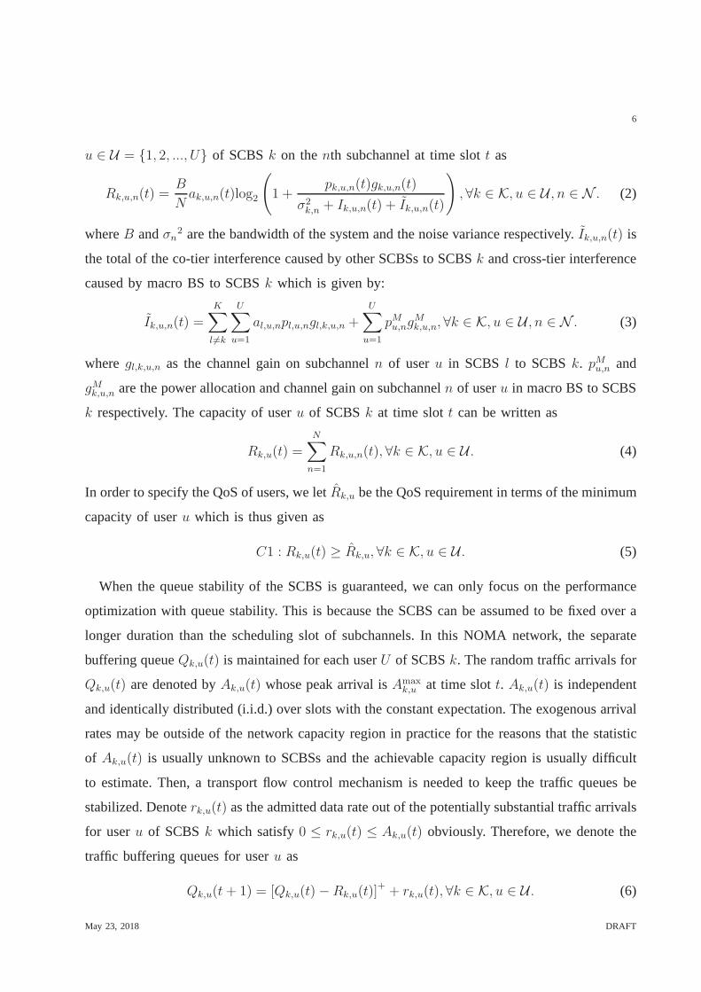
u ∈ U = {1, 2, ..., U} of SCBSk on thenth subchannel at time slott as
Rk,u,n(t) =B
Nak,u,n(t)log2
(1 +
pk,u,n(t)gk,u,n(t)
σ2k,n + Ik,u,n(t) + Ik,u,n(t)
), ∀k ∈ K, u ∈ U , n ∈ N . (2)
whereB andσn2 are the bandwidth of the system and the noise variance respectively. Ik,u,n(t) is
the total of the co-tier interference caused by other SCBSs to SCBSk and cross-tier interference
caused by macro BS to SCBSk which is given by:
Ik,u,n(t) =
K∑
l 6=k
U∑
u=1
al,u,npl,u,ngl,k,u,n +
U∑
u=1
pMu,ngMk,u,n, ∀k ∈ K, u ∈ U , n ∈ N . (3)
wheregl,k,u,n as the channel gain on subchanneln of useru in SCBS l to SCBSk. pMu,n and
gMk,u,n are the power allocation and channel gain on subchanneln of useru in macro BS to SCBS
k respectively. The capacity of useru of SCBSk at time slott can be written as
Rk,u(t) =N∑
n=1
Rk,u,n(t), ∀k ∈ K, u ∈ U . (4)
In order to specify the QoS of users, we letRk,u be the QoS requirement in terms of the minimum
capacity of useru which is thus given as
C1 : Rk,u(t) ≥ Rk,u, ∀k ∈ K, u ∈ U . (5)
When the queue stability of the SCBS is guaranteed, we can only focus on the performance
optimization with queue stability. This is because the SCBScan be assumed to be fixed over a
longer duration than the scheduling slot of subchannels. Inthis NOMA network, the separate
buffering queueQk,u(t) is maintained for each userU of SCBSk. The random traffic arrivals for
Qk,u(t) are denoted byAk,u(t) whose peak arrival isAmaxk,u at time slott. Ak,u(t) is independent
and identically distributed (i.i.d.) over slots with the constant expectation. The exogenous arrival
rates may be outside of the network capacity region in practice for the reasons that the statistic
of Ak,u(t) is usually unknown to SCBSs and the achievable capacity region is usually difficult
to estimate. Then, a transport flow control mechanism is needed to keep the traffic queues be
stabilized. Denoterk,u(t) as the admitted data rate out of the potentially substantialtraffic arrivals
for useru of SCBSk which satisfy0 ≤ rk,u(t) ≤ Ak,u(t) obviously. Therefore, we denote the
traffic buffering queues for useru as
Qk,u(t+ 1) = [Qk,u(t)−Rk,u(t)]+ + rk,u(t), ∀k ∈ K, u ∈ U . (6)
May 23, 2018 DRAFT
Page 7
7
The time averaged throughput in terms of the data arrivals for users in SCBSk is defined as
rk,u = limT→∞
1T
T∑t=0
rk,u(t).
Denote bypk,u(t) andptot(t) the instantaneous power of useru of SCBSk at time slott and
the total power consumption of all the SCBSs at time slott respectively, which can be written
as
pk,u(t) =
N∑
n=1
pk,u,n(t) + pCk (7)
and
ptot(t) =
K∑
k=1
U∑
u=1
pk,u(t) (8)
where pCk accounts for the circuit power of SCBSk. The average and instantaneous power
constraints of useru of SCBSk are denoted byPk,u and Pk,u, which can be written as
pk,u = limt→∞
1
t
t∑
τ=0
pk,u(τ) ≤ Pk,u, ∀k ∈ K, u ∈ U (9)
pk,u(t) ≤ Pk,u, ∀k ∈ K, u ∈ U . (10)
We define the functiongR(·) as the revenue obtained by the throughput which is a non-
decreasing concave utility function. LetηEE denote the energy efficiency (EE) which is defined as
the ratio of the profit brought by the long-term utility of average throughput to the corresponding
long-term total power consumption. It can be written as
ηEE =
K∑k=1
U∑u=1
gR (rk,u)
ptot. (11)
whereptot = limT→∞
1T
T∑t=0
ptot(t).
C. Optimization Problem Formulation
In this subsection, when considering all constraints, the utility function is expressed as
maxP
ηEE =
K∑k=1
U∑u=1
gR(rk,u)
ptot
s.t.C1
C2 : pk,u = limt→∞
1t
t∑τ=0
pk,u(τ) ≤ Pk,u, ∀k ∈ K, u ∈ U
C3 : pk,u(t) ≤ Pk,u, ∀k ∈ K, u ∈ U
C4 : Rk,u = limT→∞
1T
T∑t=0
Rk,u(t) ≥ rk,u, ∀k ∈ K, u ∈ U .
(12)
May 23, 2018 DRAFT
Page 8
8
whereP denotes the power allocation policy and the constraintC1 ensures the QoS of users;
C2 is limit of the maximum average transmit power of useru of SCBSk; C3 is the maximum
instantaneous transmit power of useru of SCBSk; andC4 ensures the stability of useru in
SCBSk. We define the optimal EEηoptEE as
ηoptEE =
K∑k=1
U∑u=1
gR (rk,u(P∗))
ptot(P∗)= max
P
K∑k=1
U∑u=1
gR (rk,u(P))
ptot(P)(13)
whereP∗ denotes the optimal power allocation policy that yieldsηoptEE. We can classify the utility
function in (12) as a nonlinear fractional program. We introduce Theorem 1 as follows.
Theorem 1: The optimal EEηoptEE can be reached if and only if
maxP
K∑k=1
U∑u=1
gR (rk,u(P))− ηoptEEptot(P)
=K∑k=1
U∑u=1
gR (rk,u(P∗))− ηoptEE ptot(P∗) = 0
forK∑k=1
U∑u=1
gR (rk,u(P)) ≥ 0, ptot(P) ≥ 0.
(14)
Proof: Please refer to Appendix A.
According to Theorem 1, an equivalent objective function insubtractive form is existed for the
(non-convex) optimization problem (12) which can be classified as nonlinear fractional program.
Then, the formulation (12) can be rewritten in the more tractable form
maxP
K∑k=1
U∑u=1
gR (rk,u(P))− ηEEptot(P)
s.t.C1, C2, C3, C4.
(15)
III. ENERGY EFFICIENT OPTIMIZATION USING LYAPUNOV OPTIMIZATION
In this section, the subchannel assignment is investigatedin the NOMA network and the
optimization problem in (15) is solved based on Lyapunov optimization.
A. Subchannel Matching
We assume that all the users of BS can transmit on the subchannel n arbitrarily at time slot
t in a NOMA system. Considering the complexity of decoding andthe fairness of users, each
subchannel can only be allocated to at mostDn users and each user can only occupy at most
Du subchannels at the same time. We assume thatN ∗Dn ≥ U ∗ Du. The dynamic matching
May 23, 2018 DRAFT
Page 9
9
between the users and the subchannels of SCBSk is considered as a many-many matching
process between the set ofU users and the set ofN subchannels. Useru is matched with
subchanneln at time slott if ak,u,n(t) = 1. Based on the channel state information, we assume
useru prefers channeln1 over n2 if and only if gk,u,n1> gk,u,n2
. Then, the preference lists of
the users of SCBSk can be denoted by
Pr ef (K,U) = [Pr ef U(1), ...,Pr ef U(u), ...Pr ef U(U)]T (16)
wherePr ef (K,U)(u) is the preference list of useru of SCBSk which is in the descending
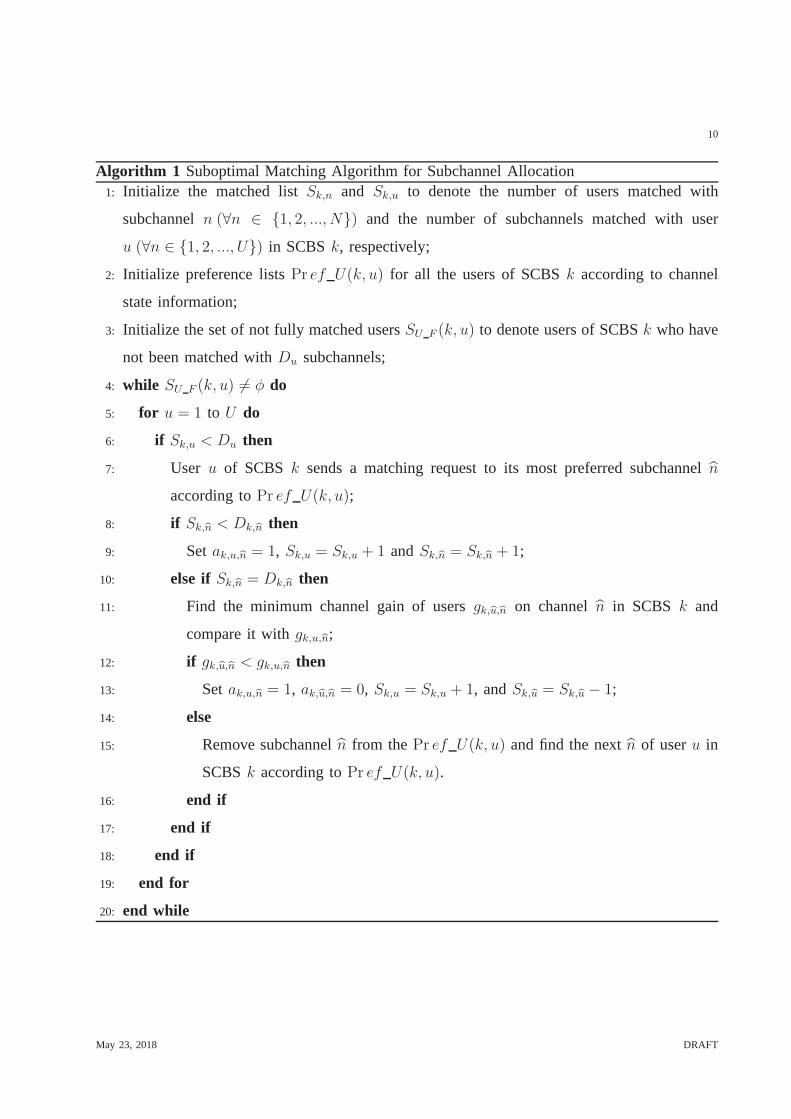
order of channel gains of subchannels. To reduce the complexity, we propose a suboptimal
matching algorithm for subchannel allocation as Algorithm1. For each useru of SCBS k,
the matching request is send to its most preferred subchannel according to its preference list.
Then the preferred subchannel decides whether accept the user or not according to the users’s
channel gain. For each subchanneln, there is at mostDn number of accepted users who has
higher channel gain than the rejected users. The rejected user on subchanneln will remove
the subchanneln from its preference list and its most preferred subchannel is changed. The
matching request is send again until all the users of each SCBS matchedDu subchannels and
the matching is achieved.
B. The Queues of Lyapunov Optimization
BecausegR(rk,u) is related to the time averaged throughput, we define auxiliary variablesγk,u
for the traffic arrival of useru in SCBSk which satisfiesγk,u ≤ rk,u and 0 ≤ γk,u ≤ Amaxk,u .
Therefore, the optimization problem in (15) can be rewritten as
maxP
∑k∈K
∑u∈U
gR(γk,u)− ηEEptot
s.t.C1,C2,C3,C4
C5 : γk,u ≤ rk,u, 0 ≤ γk,u ≤ Amaxk,u
(17)
where γk,u = limT→∞
1T
T∑t=0
γk,u(t) and gR(γk,u)− ηEEptot = limT→∞
1T
T∑t=0
(gR(γk,u(t))− ηEEptot).
The equivalent of problems (15) and (17) can be proved by appendix B. To satisfy the averaged
throughput constraint inC5, we denote byHk,u(t) the virtual queue for useru in SCBSk at
time slot t. We get
Hk,u(t + 1) = [Hk,u(t)− rk,u(t)]+ + γk,u(t), ∀k ∈ K, u ∈ U . (18)
May 23, 2018 DRAFT
Page 10
10
Algorithm 1 Suboptimal Matching Algorithm for Subchannel Allocation1: Initialize the matched listSk,n and Sk,u to denote the number of users matched with
subchanneln (∀n ∈ {1, 2, ..., N}) and the number of subchannels matched with user
u (∀n ∈ {1, 2, ..., U}) in SCBSk, respectively;
2: Initialize preference listsPr ef U(k, u) for all the users of SCBSk according to channel
state information;
3: Initialize the set of not fully matched usersSU F (k, u) to denote users of SCBSk who have
not been matched withDu subchannels;
4: while SU F (k, u) 6= φ do
5: for u = 1 to U do
6: if Sk,u < Du then
7: User u of SCBS k sends a matching request to its most preferred subchanneln
according toPr ef U(k, u);
8: if Sk,n < Dk,n then
9: Setak,u,n = 1, Sk,u = Sk,u + 1 andSk,n = Sk,n + 1;
10: else if Sk,n = Dk,n then
11: Find the minimum channel gain of usersgk,u,n on channeln in SCBS k and
compare it withgk,u,n;
12: if gk,u,n < gk,u,n then
13: Setak,u,n = 1, ak,u,n = 0, Sk,u = Sk,u + 1, andSk,u = Sk,u − 1;
14: else
15: Remove subchanneln from thePr ef U(k, u) and find the nextn of useru in
SCBSk according toPr ef U(k, u).
16: end if
17: end if
18: end if
19: end for
20: end while
May 23, 2018 DRAFT
Page 11
11
Similarly, in order to satisfy the constraintC2, virtual power queues for the useru in SCBS
k are defined. We denoteZk,u(t) as the queue arrival with the transmit powerpk,u(t), and get
Zk,u(t + 1) = [Zk,u(t)− Pk,u]+ + pk,u(t), ∀k ∈ K, u ∈ U . (19)
C. The Formulation of Lyapunov Optimization
DenoteΦ(t) = [Q(t), H(t), Z(t)] as the matrix of all the queues. We define the Lyapunov
function as a scalar metric of queue congestion
L (Φ (t)) =1
2
{K∑
k=1
U∑
u=1
(Qk,u(t)
2 +Hk,u(t)2 + Zk,u(t)
2)}. (20)
We introduce a Lyapunov drift in this subsection for pushingthe Lyapunov function to a lower
congestion state and keep both the actual and virtual queuesstable
∆(Φ(t)) = E {L(Φ(t + 1))− L(Φ(t))} . (21)
According to Lyapunov optimization, by subtractingV E
{∑u∈U
gR(γk,u)− ηEEptot
}from both
sides of (21), we get
∆(Φ (t))− V E
{K∑k=1
U∑u=1
gR (γk,u)− ηEEptot
}
≤ C +K∑k=1
U∑u=1
E {Hk,u(t)γk,u − V gR (γk,u)}
+V E
(ηEE
{K∑k=1
{U∑
u=1
pk,u(t) + pCk
}})
−K∑k=1
U∑u=1
{Hk,u(t)−Qk,u(t)}E {rk,u(t)}−K∑k=1
U∑u=1
Qk,u(t)E {Rk,u(t)}
−K∑k=1
U∑u=1
Zk,u(t)E {Pk,u(t)− pk,u(t)}
(22)
whereV is an arbitrarily positive control parameter which represents the emphasis on utility
maximization compared to queue stability andC is a finite constant that satisfies
C ≥ 12E
{K∑k=1
U∑u=1
(rk,u(t)
2 +Rk,u(t)2)}
+12E
{K∑k=1
U∑u=1
[(rk,u(t)− γk,u(t))
2 + (Pk,u(t)− pk,u(t))2]}.
(23)
May 23, 2018 DRAFT
Page 12
12
1) The solution of virtual variables:The optimal choice ofγu to minimize (22) can be made
by solving
max V gR(γk,u)−Hk,u(t)γk,u
s.t.0 ≤ γk,u ≤ Amaxk,u
(24)
and the solution is
γk,u(t) = min
{V
Hk,u(t), Amax
k,u
}. (25)
2) The solution of actual traffic arrival:In order to minimize (22), the optimal actual traffic
arrival can be achieved by maximizing the expression as follows:
max {Hk,u(t)−Qk,u(t)}E {rk,u(t)}
s.t.0 ≤ rk,u(t) ≤ Ak,u(t).(26)
We get the optimal solution as
rk,u(t) =
Ak,u(t), ifHk,u(t)−Qk,u(t) ≻ 0
0, else.(27)
3) Power allocations:In order to minimize (22), we first obtain the optimal solution of the
virtual variables and the actual traffic arrival, then we canminimize the remaining part of (22)
and denote it as
min
V E
(ηEE
{K∑k=1
{U∑
u=1
pk,u(t) + pCk
}})+
K∑k=1
U∑u=1
Zk,u(t)pk,u(t)
−K∑k=1
U∑u=1
Qk,u(t)E {Rk,u(t)}
= V E
(ηEE
{K∑k=1
{U∑
u=1
N∑n=1
ak,u,n(t)pk,u,n(t)
}+ pCk
})
+K∑k=1
U∑u=1
Zk,u(t)
{N∑
n=1
ak,u,n(t)pk,u,n(t)
}
−K∑k=1
U∑u=1
Qk,u(t)E
{N∑
n=1
Rk,u,n(t)
}.
(28)
Let ωk,u,n(t) = ak,u,n(t)pk,u,n(t), ∀k ∈ K, u ∈ U , n ∈ N ; then we can get
Rk,u,n(t) =B
Nak,u,n(t)log2
1 +
ωk,u,n(t)gk,u,n(t)
ak,u,n(t)(σ2k,n + Ik,u,n(t) + Ik,u,n(t)
)
. (29)
May 23, 2018 DRAFT
Page 13
13
Then, we can rewrite (28) as follows
minV E
(ηEE
{K∑k=1
U∑u=1
pk,u(t)
})−
K∑k=1
{U∑
u=1
Qk,u(t)E {Rk,u(t)}+U∑
u=1
Zk,u(t)pk,u(t)
}
= V E
(ηEE
{K∑k=1
U∑u=1
N∑n=1
ωk,u,n(t)
})+
K∑k=1
U∑u=1
Zk,u(t)
{N∑
n=1
ωk,u,n(t)
}
−K∑k=1
U∑u=1
Qk,u(t)E
{BN
N∑n=1
ak,u,n(t)log2
(1 +
ωk,u,n(t)gk,u,n(t)
ak,u,n(t)(σ2
k,n+Ik,u,n(t)+Ik,u,n(t))
)}(30)
Since (30) is convex, to satisfy the series of constraints, the Lagrange function of the problem
(30) can be expressed by
F (λ, β) = minL(λ, β)
= V E
(ηEE
{K∑k=1
U∑u=1
N∑n=1
ωk,u,n(t)
})+
K∑k=1
U∑u=1
Zk,u(t)
{N∑
n=1
ωk,u,n(t)
}−
K∑k=1
U∑u=1
Qk,u(t)E
{N∑
n=1
BNak,u,n(t)log2
(1 +
ωk,u,n(t)gk,u,n(t)
ak,u,n(t)(σ2
k,n+Ik,u,n(t)+Ik,u,n(t))
)}
+K∑k=1
U∑u=1
λk,u(t)
{N∑
n=1
ωk,u,n(t)− Pk,u
}
+K∑k=1
U∑u=1
βk,u(t)
{Rk,u −
N∑n=1
BNak,u,n(t)log2
(1 +
ωk,u,n(t)gk,u,n(t)
ak,u,n(t)(σ2
k,n+Ik,u,n(t)+Ik,u,n(t))
)},
(31)
where λ , β are the Lagrange multiplier vectors for the constraints in (17). Taking the first
order derivation ofF (λ, β) with respect toωk,u,n(t), we can get the optimal power allocation as
follows
pk,u,n(t) =ωk,u,n(t)
ak,u,n(t)=
BN(Qk,u(t) + βk,u(t))
ln 2(V ηEE + Zk,u(t) + λk,u(t))−
σ2k,n + Ik,u,n(t) + Ik,u,n(t)
gk,u,n(t). (32)
Based on the subgradient method [27], the master dual problem in (32) can be solved by
λl+1k,u=[λl
k,u−εl1(Pk,u −N∑
n=1
ωk,u,n(t))]+
, ∀k ∈ K, u ∈ U ;
βl+1k,u = [βl
k,u − εl2(N∑
n=1
Rk,u,n −Rk,u)]+
, ∀k ∈ K, u ∈ U.
(33)
After the time intervalT , we get the average queue lengthQ, total average capacityRave, average
power consumptionP ave and the average energy efficient EEηaveEE as
Q =1
T
T∑
t=1
K∑
k=1
U∑
u=1
Qk,u(t) (34)
Rave =1
T
T∑
t=1
Utot(t) (35)
May 23, 2018 DRAFT
Page 14
14
Algorithm 2 Lyapunov Optimization based Resource Allocation AlgorithmInitialize theak,u,n(t) using suboptimal Algorithm 1;
2: Initialize pk,u,n(t) using equal power allocation;
Initialize the value ofAmaxk,u andQk,u(t);
4: For each time slot, calculate the auxiliary variablesγk,u(t) for each time slot and admitted
traffic rk,u(t) by solving (25), (27) respectively;
repeat
6: Obtain the optimal allocation of power in the current time slot according to (32);
Update Lagrangian multipliers ofλ, β by solving (33);
8: Solve (12) using the Dinkelbach method in [1] to get the optimal value of ηEE in an
iteration way;
until Convergence or certain stopping criteria is met
10: Calculate the traffic queueQk,u(t) and the virtual queues ofHk,u(t) andZk,u(t) of next time
slot by solving (6), (18), (19) respectively.
P =1
T
T∑
t=1
K∑
k=1
U∑
u=1
pk,u(t) (36)
ηaveEE =1
T
T∑
t=1
ηEE. (37)
The above proposed approach based on Lyapunov optimizationfor solving the EE optimization
problem in (19) can be summarized in Algorithm 2.
D. Complexity Analysis
The complexity of the proposed algorithms is analyzed in this subsection. The worst-case
complexity of proposed suboptimal Algorithm 1 isO(KUN+1/2K⌊U/Dn⌋2) in which the
finding of preference lists isO(KUN). The optimal algorithm of subchannel matching can
only be obtained by searching over all possible combinations of users whose computational
complexity can be approximated asO(K [U !]Du
DnN ). It can be found from the analysis above,
proposed suboptimal subchannel matching Algorithm 1 has a much lower polynomial complexity
than the exhaustive search. In Algorithm 2, the calculationof (32) for each user in each SCBS on
May 23, 2018 DRAFT
Page 15
15
each subchannel entailsKUN operations. Then the complexity of Algorithm 2 isO(TLKUN)
whereL is the number of iterations each time slot. As the complexityof Algorithm 2 increases
with the number of users and the convergence ofEE is influenced by the control parameterV ,
the Algorithm 2 may be practical for a middle-scale realtimenetwork and the value ofV should
be well chosen. Furthermore, cellular users are always distributed in a cluster-way. Therefore,
the cellular users in a cell can be divided into several clusters, and the proposed algorithm can be
used in each cluster. Subchannels are not shared between different clusters. Since the number of
users in each cluster is small, the complexity of the proposed algorithms will be further reduced.
IV. PERFORMANCE ANALYSIS
In this section, we analyze the performance bounds of the proposed Algorithm 2 based on
the Lyapunov optimization.
A. Stability of Queues
In this work, all the actual queuesQk,u(t) and virtual queues ofHk,u(t) andZk,u(t) are mean
rate stable. We assume the expectation ofPtot(t) andUtot(t) are bound by
Pmin ≤ E {Ptot(t)} ≤ Pmax (38)
Rmin ≤ E {Utot(t)} ≤ Rmax (39)
wherePmin, Pmax, Rmin andRmax are finite constants. From the boundedness assumptions, there
is positive constantC satisfying
∆(Φ(t)) ≤ C. (40)
It can be written as
E {L(Φ(t + 1))} − E {L(Φ(t))} ≤ C. (41)
Considering telescoping sums overt ∈ {0, 1, ..., T − 1} in above inequality, we can get
E {L(Φ(T ))} − E {L(Φ(0))} ≤ TC. (42)
Using (20), we can rewrite (42) as
E{Zk,u(T )
2} ≤ 2TC + 2E {L(Φ(0))} . (43)
May 23, 2018 DRAFT
Page 16
16
Given D(|Zk,u(T )|) = E(|Zk,u(T )|2) − [E(|Zk,u(T )|)]
2 ≥ 0, we get E(|Zk,u(T )|2) ≥
[E(|Zk,u(T )|)]2. Thus we get
E(|Zk,u(T )|) ≤√
2TC + 2E {L(Φ(0))}. (44)
Taking the limitT → ∞ and dividingT at the same time, we have
limT→∞
E(|Zk,u(T )|)
T= 0. (45)
Therefore, the queues ofZk,u(T ) are mean rate stable. Similarly, we can also prove the queues
Qk,u(T ) andHk,u(T ) are mean rate stable.
B. The Utility and Average Queue Length Performance
The EE performance and the average queue length performanceobtained by Algorithm 2 is
given in Theorem 2.
Theorem 2: Utilizing the proposed optimization solution,ηEE is bounded by
ηEE ≥ ηoptEE −B
V Pmin
. (46)
The performance of the average network queue length is bounded by
Q ≤B + V (Rmax − ηoptEEPmin)
ε(47)
whereηoptEE is the theoretical maximum achievable utility of all achievable solutions.
Proof: Please refer to Appendix C.
With the consideration ofηEE ≤ ηoptEE, which naturally holds from (13), the bound of EE is
ηoptEE− BV Pmin
≤ ηEE ≤ ηoptEE. Therefore,ηEE can arbitrarily approachηoptEE by setting large enough
V to make BV Pmin
arbitrarily small. The bound of average queue backlogQ increases linearly
in V according to (47). Theorem 2 shows that there exists an[O(1/V ),O(V )] utility-backlog
tradeoff that leads to Little’s Theorem.
V. SIMULATION RESULTS AND DISCUSSION
In this section, simulation results are given to evaluate the performance of the proposed
algorithms. In the considered NOMA network, there areK SCBSs which consistsU users
distributed randomly in a circular with radius of30 m and the SCBSS are distributed randomly
in the circular of MBS whose radius is500 m. The noise power spectral density is−174
May 23, 2018 DRAFT
Page 17
17
dBm/Hz. We consider a normalized bandwidth which isB = 1 Hz. For the simulation, the
maximum average transmit power and the maximum instantaneous transmit power of userU in
SCBSk is set as2.5/U Watts and2.505/U Watts respectively. We assume the circuit power
of useru is 1 Watt. The time intervalT is set as5000 slots which means traffic arrival rates is
15 bps/Hz. We assume that each user can access only one subchannel in the OFDMA scheme.
In Fig. 2, the average queue length versus timet is evaluated under different values of control
parameterV . The user QoS requirement is set asRu = 2 bps/Hz and the maximum number
of matched subchannels of each user isDu = 2 with the maximum number of matched users
of each subchannel isDn = 2. It is shown that, the value of the average queue length increases
with time t and gradually fluctuates around a certain fixed value. And forthe same value oft,
a smaller value ofV leads to a smaller value of average queue length which satisfy with the
Theorem 2. This conclusion can also be obtained in Fig. 9.
0 200 400 600 800 10000
200
400
600
800
1000
1200
1400
1600
1800
2000
time t (slot)
Ave
rage
que
ue le
ngth
(bp
s/H
z)
V=10V=30V=50
Fig. 2. Average queue length versus simulation time length.
Fig. 3 shows the EE performance versus timet with the same constraints of Fig. 2 except
the QoS constraint isRu = 1 bps/Hz instead. It can be observed that the EE performance
will gradually fluctuates around a certain fixed value with the increase oft which illustrates the
convergence of EE with timet. And the larger value ofU lead to smaller convergence ofEE.
May 23, 2018 DRAFT
Page 18
18
0 1000 2000 3000 4000 500034
35
36
37
38
39
40
time t (slot)
Ave
rage
EE
(bi
ts/H
z/Jo
ule)
U=10U=15U=20
Fig. 3. EE performance versus simulation time length.
This is because the need of subchannels will increase with the increase of user number which
lead to the decrease of bandwidth of each subchannel.
As shown in Fig. 4, the EE performance is evaluated with the simulation time slott. In
each time slott, the algorithms in Fig. 4 have the equal total power consumption. That is, the
total power consumption is time varied for each algorithm. With the increase of timet, the
EE will gradually fluctuates around a certain fixed value. From Fig. 4, we observe that the
performance ofV = 100 which is the proposed resource allocation algorithms with the control
parameterV = 100, including subchannel assignment and power allocation, ismuch better than
the algorithm of NOMA-EQ in [16]. This is because the algorithm of NOMA-EQ is limited of
equal power allocation of each subchannel in NOMA system. For different subchannel allocation
schemes, the EE performance using exhaustive search which denoted as NOMA-Opt is better
than using the suboptimal algorithm we proposed.
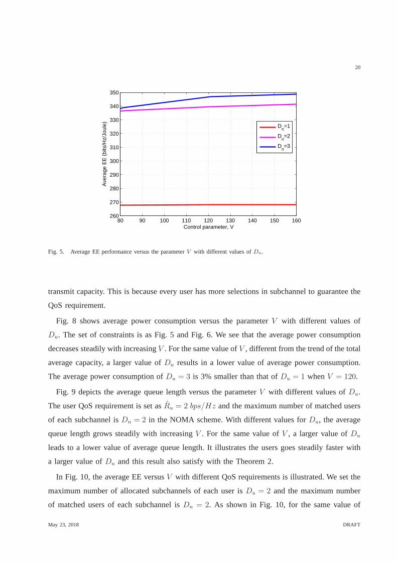
In Fig. 5, the performance of average EE is evaluated versus the parameterV with different
values ofDn which is the number of users matched with each subchannel andDn = 1 represents
it’s in a OFDMA scheme. The user QoS requirement is set asRu = 2 bps/Hz and the maximum
number of matched subchannels of each user isDu = 1. It is shown that, with the increase in
May 23, 2018 DRAFT
Page 19
19
the parameterV , the value of average EE increases and converges to a certainvalue both in
NOMA at the same value ofDu and in OFDMA. It is seen that the average EE in NOMA is
better than the average EE in OFDMA. And for the same value ofV , a larger value ofDn leads
to a larger value of average EE. This is because our proposed algorithm provides more freedom
in the bandwidth allocation of assigned subchannels. For the same set of users under same value
of Du, the more larger of the valuse ofDn is, the bandwidth of each subchannel is more larger.
0 1000 2000 3000 4000 5000 600010.5
11
11.5
12
12.5
13
13.5
14
14.5
15
15.5
time t (slot)
EE
(bi
ts/H
z/Jo
ule)
V=100NOMA−EQNOMA−Opt
Fig. 4. EE performance versus simulation time length with different algorithms.
Fig. 6 shows the performance of average EE versus the parameter V with different values
of Du where the user QoS requirement is set asRu = 2 bps/Hz and the maximum number
of matched users of each subchannel isDn = 2. It is seen that, for arbitrary value ofDu, the
value of average EE Arbitrary increases and converges to a certain value with the increase in the
parameterV . For the same value of parameterV , a larger value ofDu leads to a larger value
of average EE due to the various selection of subchannels.
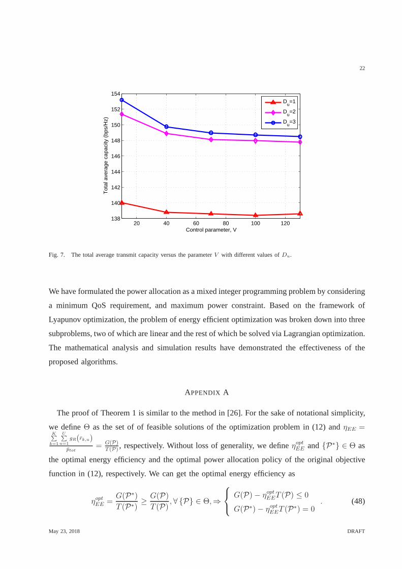
Fig. 7 illustrates the convergence of the total average capacity versus the parameterV with
different values ofDu. Different from the trend of average EE, for the same value ofDu, the
value of the total average transmit capacity decreases and converges to a value with the increase
of V . For the same value ofV , a larger value ofDu results in a larger value of total average
May 23, 2018 DRAFT
Page 20
20
80 90 100 110 120 130 140 150 160260
270
280
290
300
310
320
330
340
350
Control parameter, V
Ave
rage
EE
(bi
ts/H
z/Jo
ule)
Dn=1
Dn=2
Dn=3
Fig. 5. Average EE performance versus the parameterV with different values ofDn.
transmit capacity. This is because every user has more selections in subchannel to guarantee the
QoS requirement.
Fig. 8 shows average power consumption versus the parameterV with different values of
Du. The set of constraints is as Fig. 5 and Fig. 6. We see that the average power consumption
decreases steadily with increasingV . For the same value ofV , different from the trend of the total
average capacity, a larger value ofDu results in a lower value of average power consumption.
The average power consumption ofDu = 3 is 3% smaller than that ofDu = 1 whenV = 120.
Fig. 9 depicts the average queue length versus the parameterV with different values ofDu.
The user QoS requirement is set asRu = 2 bps/Hz and the maximum number of matched users
of each subchannel isDn = 2 in the NOMA scheme. With different values forDu, the average
queue length grows steadily with increasingV . For the same value ofV , a larger value ofDu
leads to a lower value of average queue length. It illustrates the users goes steadily faster with
a larger value ofDu and this result also satisfy with the Theorem 2.
In Fig. 10, the average EE versusV with different QoS requirements is illustrated. We set the
maximum number of allocated subchannels of each user isDu = 2 and the maximum number
of matched users of each subchannel isDn = 2. As shown in Fig. 10, for the same value of
May 23, 2018 DRAFT
Page 21
21
20 40 60 80 100 12028
29
30
31
32
33
34
35
36
Control parameter, V
Ave
rage
EE
(bi
ts/H
z/Jo
ule)
Du=1
Du=2
Du=3
Fig. 6. Average EE performance versus the parameterV with different values ofDu.
V , a larger value of the QoS requirement results in a smaller converged value of average EE.
A smaller value of QoS requirement leads to a larger value of EE due to the fact that a smaller
value of QoS requirement enlarges the feasible region of theoptimizing variable.
Fig. 11 shows the average power consumption versusV with different QoS requirements. The
maximum number of allocated subchannels of each user isDu = 2 and the maximum number
of matched users of each subchannel isDn = 2. As the parameterV increases, average power
consumption continues to decrease. From Fig. 11, we can observe that for the same value ofV ,
a larger value of the QoS requirement results in a larger value of average power consumption.
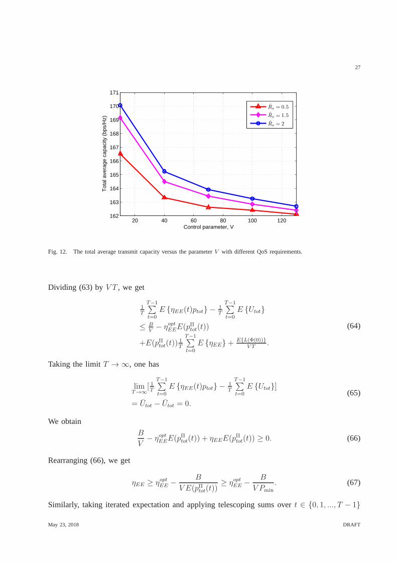
In Fig. 12, the total average transmit capacity is evaluatedversusV with different QoS
requirements. The mean traffic arrival rateα = 15 bps/Hz and has the same constraints of Fig.
11. It can be observed that, the trend of this curve is similarto the average power consumption
curves in Fig. 11. For the same parameterV , a larger value of the QoS requirement results in
a larger value of the total average transmit capacity.
VI. CONCLUSION
We have investigated dynamic resource allocation in downlink NOMA networks. We have
proposed a suboptimal subchannel assignment algorithm based on the two-side matching method.
May 23, 2018 DRAFT
Page 22
22
20 40 60 80 100 120138
140
142
144
146
148
150
152
154
Control parameter, V
Tot
al a
vera
ge c
apac
ity (
bps/
Hz)
D
u=1
Du=2
Du=3
Fig. 7. The total average transmit capacity versus the parameterV with different values ofDu.
We have formulated the power allocation as a mixed integer programming problem by considering
a minimum QoS requirement, and maximum power constraint. Based on the framework of
Lyapunov optimization, the problem of energy efficient optimization was broken down into three
subproblems, two of which are linear and the rest of which be solved via Lagrangian optimization.
The mathematical analysis and simulation results have demonstrated the effectiveness of the
proposed algorithms.
APPENDIX A
The proof of Theorem 1 is similar to the method in [26]. For thesake of notational simplicity,
we defineΘ as the set of of feasible solutions of the optimization problem in (12) andηEE =K∑
k=1
U∑u=1
gR(rk,u)
ptot= G(P)
T (P), respectively. Without loss of generality, we defineηoptEE and{P∗} ∈ Θ as
the optimal energy efficiency and the optimal power allocation policy of the original objective
function in (12), respectively. We can get the optimal energy efficiency as
ηoptEE =G(P∗)
T (P∗)≥
G(P)
T (P), ∀ {P} ∈ Θ,⇒
G(P)− ηoptEET (P) ≤ 0
G(P∗)− ηoptEET (P∗) = 0
. (48)
May 23, 2018 DRAFT
Page 23
23
20 40 60 80 100 1204.1
4.2
4.3
4.4
4.5
4.6
4.7
4.8
4.9
Control parameter, V
Ave
rage
pow
er c
onsu
mpt
ion
(W)
Du=1
Du=2
Du=3
Fig. 8. The average power consumption versus the parameterV with different values ofDu.
Therefore, we can conclude thatmaxp
G(P) − ηoptEET (P) = 0 is achievable by power allocation
policy {P∗} which completes the forward implication.
Then, the converse implication of Theorem 1 is proved as below. SupposeP∗◦ is the optimal
power allocation policy of the equivalent objective function such that
G(P∗◦ )− ηoptEET (P
∗◦ ) = 0 (49)
Then, for any feasible power allocation policy{P} ∈ Θ, we can obtain the following inequality
G(P)− ηoptEET (P) ≤ G(P∗◦ )− ηoptEET (P
∗◦ ) = 0. (50)
The above inequality impliesG(P)
T (P)≤ ηoptEE, ∀ {P} ∈ Θ (51)
andG(P∗
◦ )
T (P∗◦ )
= ηoptEE (52)
It implies the optimal power allocation policy{P∗◦} for the equivalent objective function is also
the optimal resource allocation policy for the original objective function.
May 23, 2018 DRAFT
Page 24
24
20 40 60 80 100 1200
1000
2000
3000
4000
5000
6000
7000
Control parameter, V
Ave
rage
que
ue le
ngth
(bp
s/H
z)
D
u=1
Du=2
Du=3
Fig. 9. The average queue length versus the parameterV with different values ofDu.
APPENDIX B
We denoteY1 and Y2 be the optimal utility of problems (15) and (17), respectively. The
optimal solutions that achieveY1 and Y2 are denoted byX1 and X2, respectively. Since the
utility functions of (15) and (17) are non-decreasing concave function which can be expressed
asU (·), by Jensen’s inequality, we have
U(X2
)≥ U(X2) = Y2 (53)
Due to the the solutionX2 satisfies the constraintC5, we can get
U(X1
)≥ U
(X2
)(54)
Moreover, sinceX2 also satisfies the constraints of the problem (15), then we have
Y1 ≥ U(X1
)≥ Y2 (55)
For X1 is an optimal solution to the problem (15), it also satisfies the constraintsC1− C4. By
choosingX2 = X1 at each slot, then we get
Y2 ≥ U(X2) = U(X1
)= Y1 (56)
Therefore,Y1 = Y2 is proved and we can further conclude the equivalence of the problems (15)
and (17).
May 23, 2018 DRAFT
Page 25
25
20 40 60 80 100 12030
31
32
33
34
35
36
37
38
39
Control parameter, V
Ave
rage
EE
(bi
ts/H
z/Jo
ule)
Ru = 0.5
Ru = 1.5
Ru = 2
Fig. 10. Average EE performance versus the parameterV with different QoS requirements.
APPENDIX C
PROOF OFTHEOREM 2
To prove the bounds on the EE and the average queue length, Lemma 1 is introduced below.
Lemma 1: For arbitrary arrival rates, a randomized stationary control policy Π exists and it
chooses feasible control decision independent of current traffic queues and virtual queues. We
get the following steady state values:
E[rΠu (t)] = r∗u (57)
E[RΠu (t)] ≥ E[rΠu (t)] + ε = r∗u + ε (58)
E[Pu − pΠu (t)] ≤ δ (59)
E[UΠtot(t)] ≥ E[pΠtot(t)](η
optEE − δ). (60)
Proof: The proof of Lemma 1 is similar to one found in [28].
May 23, 2018 DRAFT
Page 26
26
20 40 60 80 100 1204
4.2
4.4
4.6
4.8
5
5.2
5.4
5.6
Control parameter, V
Ave
rage
pow
er c
onsu
mpt
ion
(W)
Ru = 0.5
Ru = 1.5
Ru = 2
Fig. 11. The average power consumption versus the parameterV with different QoS requirements.
Substituting (57)-(60) into (22) and taking a limitδ → 0, we can get
∆(Φ(t))− V E
{∑u∈U
gR(γu)− ηEEptot
}
≤ B − V ηoptEEE(pΠtot(t)) + V ηEEE(pΠtot(t))
−ε∑u∈U
Qu(t).
(61)
For Qu(t) ≥ 0, the inequality (61) can be further simplified to
∆(Φ(t))− V E
{∑u∈U
gR(γu)− ηEEptot
}
≤ B − V ηoptEEE(pΠtot(t))
+V ηEEE(pΠtot(t)).
(62)
Using telescoping sums overt ∈ {0, 1..., T − 1} and taking iterated expectation, we have
E {L(Φ(T ))} − E {L(Φ(0))}
−V E {Utot − ηEE(t)ptot}
≤ T [B − V ηoptEEE(pΠtot(t))}
+V E(pΠtot(t))T−1∑t=0
E {ηEE}.
(63)
May 23, 2018 DRAFT
Page 27
27
20 40 60 80 100 120162
163
164
165
166
167
168
169
170
171
Control parameter, V
Tot
al a
vera
ge c
apac
ity (
bps/
Hz)
Ru = 0.5
Ru = 1.5
Ru = 2
Fig. 12. The total average transmit capacity versus the parameterV with different QoS requirements.
Dividing (63) by V T , we get
1T
T−1∑t=0
E {ηEE(t)ptot} −1T
T−1∑t=0
E {Utot}
≤ BV− ηoptEEE(pΠtot(t))
+E(pΠtot(t))1T
T−1∑t=0
E {ηEE}+E{L(Φ(0))}
V T.
(64)
Taking the limitT → ∞, one has
limT→∞
[ 1T
T−1∑t=0
E {ηEE(t)ptot} −1T
T−1∑t=0
E {Utot}]
= Utot − Utot = 0.
(65)
We obtain
B
V− ηoptEEE(pΠtot(t)) + ηEEE(pΠtot(t)) ≥ 0. (66)
Rearranging (66), we get
ηEE ≥ ηoptEE −B
V E(pΠtot(t))≥ ηoptEE −
B
V Pmin
. (67)
Similarly, taking iterated expectation and applying telescoping sums overt ∈ {0, 1, ..., T − 1}
May 23, 2018 DRAFT
Page 28
28
to (61), we get
E {L(Φ(T ))} − E {L(Φ(0))}
−V E {Utot − ηEE(t)ptot(t)}
≤ T [B − V ηoptEEE(pΠtot(t))]
−εT−1∑t=0
[∑k∈K
∑u∈U
E {Qu(t)}]
+V E(pΠtot(t))T−1∑t=0
E {ηEE}.
(68)
Dividing (68) by εT and taking a limit asT → ∞, we obtain
Q = limT→∞
1T
T−1∑t=0
[∑u∈U
E {Qu(t)}]
≤
B−V ηopt
EEE(pΠtot(t))
ε
+Vε
limT→∞
1T
T−1∑t=0
E {ηEE(t)ptot(t)}
≤B+V (Rmax−η
optEE
Pmin)
ε.
(69)
REFERENCES
[1] D. W. K. Ng, E. S. Lo, and R. Schober, “Energy-efficient resource allocation in multi-cell OFDMA systems with limited
backhaul capacity,”IEEE Trans. Wireless Commun., vol. 11, no. 10, pp. 3618–3631, Sep. 2012.
[2] D. Yuan, J. Joung, C. K. Ho, and S. Sun, “On tractability aspects of optimal resource allocation in OFDMA systems,”
IEEE Trans. Veh. Technol., vol. 62, no. 2, pp. 863–873, Feb. 2013.
[3] Y. Saito, Y. Kishiyama, A. Benjebbour, T. Nakamura, A. Li, and K. Higuchi, “Non-orthogonal multiple Access (NOMA)
for cellular future radio access,”Proc. IEEE 77th Veh. Technol. Conf., vol. 53, no. 3, pp. 1–5, June 2013.
[4] Z. Ding, F. Adachi, and H. V. Poor, “The application of MIMO to non-orthogonal multiple access,”IEEE Trans. Wireless
Commun., vol. 15, no. 11, pp. 537–552, Jan. 2016.
[5] Z. Yang, J. Cui, X. Lei, Z. Ding, P. Fan, and D. Chen, “Impact of factor graph on average sum rate for uplink sparse code
multiple access systems,”IEEE Access, vol. 4, pp. 6585–6590, Jan. 2016.
[6] L. Dai, B. Wang, Y. Yuan, S. Han, C. I, and Z. Wang, “Non-orthogonal multiple access for 5G: Solutions, challenges,
opportunities, and future research trends,”IEEE Commun. Mag., vol. 53, no. 9, pp. 74–81, Sep. 2015.
[7] Z. Wei, J. Yuan, D. W. K. Ng, M. Elkashlan, Z. Ding, “A survey of downlink non-orthogonal multiple access for 5G
wireless communication networks,”ZTE Commun., 2016.
[8] Z. Ding, P. Fan, and H. V. Poor, “Impact of user pairing on 5G nonorthogonal multiple-access downlink transmissions,”
IEEE Trans. Veh. Technol., vol. 65, no. 8, pp. 6010–6023, Aug. 2016.
[9] Z. Ding, M. Peng, and H. V. Poor, “Cooperative non-orthogonal multiple access in 5G systems,”IEEE Commun. Lett.,
vol. 19, no. 8, pp. 1462–1465, Aug. 2015.
[10] K. Higuchi and A. Benjebbour, “Non-orthogonal multiple access (NOMA) with successive interference cancellationfor
future radio access,”IEICE Trans. Commun., vol. 98, no. 3, pp. 403–414, Mar. 2015.
[11] N. Jindal, S. Vishwanath, and A. Goldsmith, “On the duality of Gaussian multiple-access and broadcast channels,”IEEE
Trans. Inf. Theory, vol. 50, no. 5, pp. 768–783, May. 2004.
May 23, 2018 DRAFT
Page 29
29
[12] Z. Ding, Z. Yang, P. Fan, and H. Poor, “On the performanceof non-orthogonal multiple access in 5G systems with
randomly deployed users,”IEEE Signal Process. Lett., vol. 21, no. 12, pp. 1501–1505, Dec. 2014.
[13] M. F. Hanif, Z. Ding, T. Ratnarajah, and G. K. Karagiannidis, “A minorization-maximization method for optimizing sum
rate in the downlink of non-orthogonal multiple access systems,” IEEE Trans. Signal Process., vol. 64, no. 1, pp. 76–88,
Jan. 2016.
[14] S. Timotheou and I. Krikidis, “Fairness for non-orthogonal multiple access in 5G systems,”IEEE Signal Process. Lett.,
vol. 22, no. 10, pp. 1647–1651, Oct. 2015.
[15] Y. Zhang, H. M. Wang, T. X. Zheng, and Q. Yang, “Energy-efficient transmission design in non-orthogonal multiple
access,”IEEE Trans. Veh. Technol., vol. 66, no. 3, pp. 2852–2857, Mar. 2017.
[16] F. Fang, H. Zhang, J. Cheng, and V. C. M. Leung, “Energy-efficient resource allocation for downlink non-orthogonal
multiple access network,”IEEE Trans. Commun., vol. 64, no. 9, pp. 3722–3732, July 2016.
[17] M. Mollanoori and M. Ghaderi, “Uplink scheduling in wireless networks with successive interference cancellation,” IEEE
Trans. Mobile Comput., vol. 13, no. 5, pp. 1132–1144, May 2014.
[18] M. Al-Imari, P. Xiao, M. Imran, and R. Tafazolli, “Uplink non-orthogonal multiple access for 5G wireless networks,” IEEE
ISWCS, pp. 781–785, Aug. 2014.
[19] B. Wang, L. Dai, Z. Wang, N. Ge, and S. Zhou, “Spectrum andenergy-efficient beamspace MIMO-NOMA for millimeter-
wave communications using lens antenna array,”IEEE J. Sel. Areas Commun., vol. 35, no. 10, pp. 2370–2382, July
2017.
[20] L. Qian, Y. Wu, H. Zhou, and X. Shen, “Non-orthogonal multiple access vehicular small cell networks: Architecture and
solution,” IEEE Netw., vol. 31, no. 4, pp. 15–21, Aug. 2017.
[21] J. Zhao, Y. Liu, K. K. Chai, A. Nallanathan, Y. Chen, and Z. Han, “Spectrum allocation and power control for non-
orthogonal multiple access in HetNets,”IEEE Trans. Wireless Commun., vol. 16, no. 9, pp. 5825–5837, Sep. 2017.
[22] J. Li, M. Peng, Y. Yu, and Z. Ding, “Energy-efficient joint congestion control and resource optimization in heterogeneous
cloud radio access networks,”IEEE Trans. Veh. Technol., vol. 65, no. 12, pp. 9873–9887, Dec. 2016.
[23] Y. Yu, M. Peng, J. Li, A. Cheng, and C. Wang, “Resource allocation optimization for hybrid access mode in heterogeneous
networks,” IEEE Wireless Communications and Networking Conference (WCNC), pp. 1243–1248, Mar. 2015.
[24] Q. Chen, G. Yu, R. Yin, A. Maaref, G. Y. Li, and A. Huang, “Energy efficiency optimization in licensed-assisted access,”
IEEE J. Sel. Areas Commun., vol. 34, no. 4, pp. 723–734, Apr. 2016.
[25] L. Lei, D. Yuan, C. K. Ho, S. Sun, “Power and channel allocation for non-orthogonal multiple access in 5G systems:
Tractability and computation,”IEEE Trans. Wireless Commun., vol. 15, no. 12, pp. 8580–8594, Sep. 2016.
[26] W. Dinkelbach, “On nonlinear fractional programming,” Management Science, vol. 13, pp. 492–498, Mar. 1967. Available:
http://www.jstor.org/stable/2627691
[27] S. Boyd and L. Vandenberghe,Convex Optimization. Cambridge University Press, 2004.
[28] Y. Li, M. Sheng, Y. Shi, X. Ma, and W. Jia, “Energy efficiency and delay tradeoff for time-varying and interference-free
wireless networks,”IEEE Trans. Wireless Commun., vol. 13, no. 11, pp. 5921–5931, Nov. 2014.
May 23, 2018 DRAFT