

Diffusion impedance
0 0.5 1Re Z
0
0.5
Im
Z
Erase
August 29, 2001

ER@SE/August 29, 2001 2

Contents
1 Nernst condition 51.1 General diffusion equations . . . . . . . . . . . . . . . . . . . . . 51.2 Semi-infinite diffusion condition . . . . . . . . . . . . . . . . . . . 6
1.2.1 Semi-infinite linear diffusion conditiond = 1, ∆c(∞) = 0 . . . . . . . . . . . . . . . . . . . . . . 6
1.2.2 Semi-infinite radial cylindrical diffusion conditiond = 2, ∆c(∞) = 0 . . . . . . . . . . . . . . . . . . . . . . 7
1.2.3 Semi-infinite spherical diffusion conditiond = 3, ∆c(∞) = 0 . . . . . . . . . . . . . . . . . . . . . . 8
1.3 Bounded diffusion condition (linear diffusion) ∆c(rδ) = 0 . . . . 91.3.1 Randles circuit . . . . . . . . . . . . . . . . . . . . . . . . 91.3.2 Modified bounded diffusion impedance # 1 . . . . . . . . 101.3.3 Modified finite diffusion impedance # 2 . . . . . . . . . . 11
1.4 Radial cylindrical diffusion d = 2 . . . . . . . . . . . . . . . . . . 111.4.1 Finite outside cylinder . . . . . . . . . . . . . . . . . . . . 121.4.2 Infinite outside cylinder . . . . . . . . . . . . . . . . . . . 12
1.5 Spherical diffusion, d = 3 . . . . . . . . . . . . . . . . . . . . . . 121.5.1 Finite outside sphere, reduced impedance # 1 . . . . . . . 121.5.2 Finite outside sphere, reduced impedance # 2 . . . . . . . 131.5.3 Infinite outside sphere . . . . . . . . . . . . . . . . . . . . 13
2 Gerischer and diffusion-reaction impedance 152.1 Gerischer and modified Gerischer impedance . . . . . . . . . . . 15
2.1.1 Gerischer impedance . . . . . . . . . . . . . . . . . . . . . 152.1.2 Modified Gerischer impedance . . . . . . . . . . . . . . . 16
2.2 Diffusion-reaction impedance . . . . . . . . . . . . . . . . . . . . 162.2.1 Reduced impedance #1 . . . . . . . . . . . . . . . . . . . 162.2.2 Reduced impedance #2 . . . . . . . . . . . . . . . . . . . 17
2.3 Appendix . . . . . . . . . . . . . . . . . . . . . . . . . . . . . . . 19
3

ER@SE/August 29, 2001 4

Chapter 1
Mass transfer by diffusion,Nernst boundary condition
1.1 General diffusion equations
From:∂∆c(x, t)
∂t= Dx1−d ∂
∂x
(xd−1 ∂∆c(x, t)
∂x
)
where ∆ denotes a smaller deviation (or excursion) from the initial steady-statevalue, d = 1 corresponds to a planar electrode, d = 2 to a cylindrical electrodeand d = 3 to a spherical electrode [2, 11] (Fig. 1.1), it is obtained using theNernstian boundary condition ∆c(rδ) = 0:
Z∗(u) ∝ ∆J(r0, iu)∆c(r0, iu)
=Id/2−1(
√iuρ)Kd/2−1(
√iu)− Id/2−1(
√iu)Kd/2−1(
√iuρ)
√iu (Id/2(
√iu)Kd/2−1(
√iuρ) + Id/2−1(
√iuρ)Kd/2(
√iu))
where u is a reduced frequency. In(z) gives the modified Bessel function of thefirst kind and order n and Kn(z) gives the modified Bessel function of the secondkind and order n [20]. In(z) and Kn(z) satisfy the differential equation:
−(y(n2 + z2
))+ z y′ + z2 y′′ = 0
r0
r∆
r0 r∆ r∆ r0
Figure 1.1: Planar difusion (left), outside [5] (or convex [9]) diffusion (ρ = rδ/r0 > 1,middle), and central (or concave) diffusion (ρ < 1, right).
5
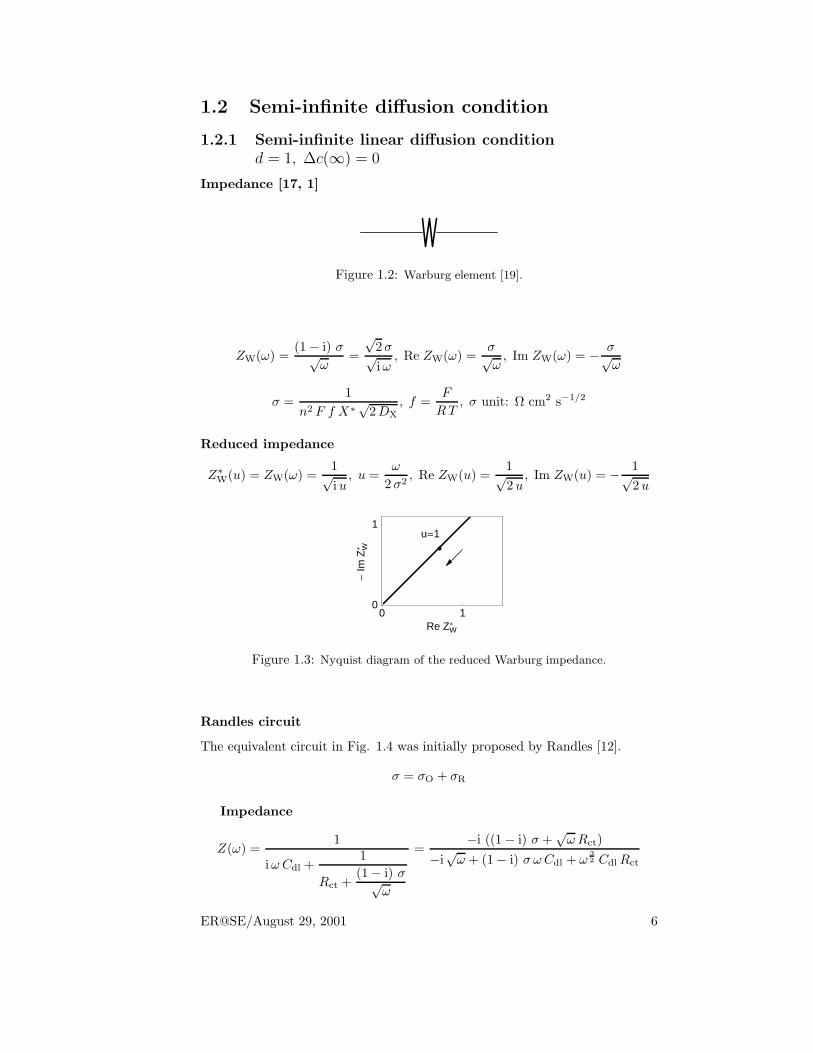
1.2 Semi-infinite diffusion condition
1.2.1 Semi-infinite linear diffusion conditiond = 1, ∆c(∞) = 0
Impedance [17, 1]
Figure 1.2: Warburg element [19].
ZW(ω) =(1− i) σ√
ω=
√2σ√iω
, Re ZW(ω) =σ√ω, Im ZW(ω) = − σ√
ω
σ =1
n2 F f X∗√2DX
, f =F
RT, σ unit: Ω cm2 s−1/2
Reduced impedance
Z∗W(u) = ZW(ω) =
1√iu
, u =ω
2 σ2, Re ZW(u) =
1√2 u
, Im ZW(u) = − 1√2 u
0 1Re ZW
0
1
Im
ZW
u1
Figure 1.3: Nyquist diagram of the reduced Warburg impedance.
Randles circuit
The equivalent circuit in Fig. 1.4 was initially proposed by Randles [12].
σ = σO + σR
Impedance
Z(ω) =1
iω Cdl +1
Rct +(1− i) σ√
ω
=−i ((1− i) σ +
√ωRct)
−i√ω + (1− i) σ ω Cdl + ω
32 Cdl Rct
ER@SE/August 29, 2001 6

Rct
Cdl
Figure 1.4: Randles circuit for semi-infinite linear diffusion.
Re Z(ω) =σ +
√ω Rct
√ω(1 + 2 σ
√ωCdl + 2 σ2 ωCdl
2 + 2 σ ω32 Cdl
2 Rct + ω2 Cdl2 Rct
2)
Im Z(ω) =−σ − 2 σ2
√ω Cdl − 2 σ ω Cdl Rct − ω
32 Cdl Rct
2
√ω(1 + 2 σ
√ωCdl + 2 σ2 ω Cdl
2 + 2 σ ω32 Cdl
2 Rct + ω2 Cdl2 Rct
2)
Reduced impedance
Z∗(u) = Z(u)/Rct =(1 + i) T (i + u)
−T√2 u+ (1 + i) (−1 + T + iu) u
u = τd ω, τd = R2ct/(2 σ2
), T = τd/τf, τf = Rct Cdl
Re Z∗(u) =T 2(−(√
2 (−1 + u))+ 2 u
32
)2√2T u (1− T + u) + 2
√u(T 2 + (−1 + T )2 u+ u3
)
Im Z∗(u) =T(√
2T (−1− u)− 2√u(1− T + u2
))2√2T u (1− T + u) + 2
√u(T 2 + (−1 + T )2 u+ u3
)
limu →0
Re Z∗(u) = 1− 1T
+1√2 u
, limu →0
Im Z∗(u) = − 1√2 u
1.2.2 Semi-infinite radial cylindrical diffusion conditiond = 2, ∆c(∞) = 0
Z∗(u) =K0(
√iu)√
iuK1(√iu)
1.2.3 Semi-infinite spherical diffusion conditiond = 3, ∆c(∞) = 0
(Fig. 1.7)
Z∗(u) =1
1 +√iu
, u = r20 ω/D
Re Z∗(u) =2 +
√2 u
2(1 +
√2 u) , Im Z∗(u) = −
√u√
2(1 +
√2 u+ u
)
ER@SE/August 29, 2001 7

0 1 2 3Re Z
0
1
2
Im
Z
a
0 11T 2 3Re Z
0
1
2
Im
Z
b
Figure 1.5: a: Nyquist diagram of the reduced impedance for the Randles circuit(Fig. 1.4). Semi-infinite linear diffusion. T = 1, 2, 5, 10, 16.4822, 102, 104. Line thick-ness increases with T . One apex for T > 16.4822. The arrows always indicate theincreasing frequency direction. b: Extrapolation of the low frequency limit plotted forT = 5.
0 Π4 2 4Re Z
0
Π41
Im
Z
Figure 1.6: Infinite outside cylindrical reduced impedance. Dot: reduced character-istic angular frequency: uc = 0.542.
1.3 Bounded diffusion condition (linear diffusion)
∆c(rδ) = 0
”Originally derived by Llopis [7], and subsequently re-derived by Sluyters [14]and Yzermans [21], Drosbach and Schultz [3], and Schuhmann [13]” [1].
• IUPAC terminology: bounded diffusion [15]
• Finite-length diffusion with transmissive boundary condition [6, 8]
Z∗Wδ
(u) =tanh
√iu√
iu, u = τd ω, τd = δ2/D, γ =
√2 u
limu→0
Z∗Wδ
(u) = 1, limu→∞
√iuZ∗
Wδ(u) = 1
Re Z∗Wδ
(γ) =sin(γ) + sinh(γ)
γ (cos(γ) + cosh(γ)), Im Z∗
Wδ(γ) =
sin(γ)− sinh(γ)γ (cos(γ) + cosh(γ))
1.3.1 Randles circuit
Impedance
Zf(u) = Rct+Rdtanh
√iu√
iu, Z(u) =
Zf(u)1 + i (u/τd)Cdl Zf(u)
, u = τd ω, τd = δ2/D
ER@SE/August 29, 2001 8

0 0.5 1Re Z
0
0.2
Im
Z uc1
Figure 1.7: Infinite outside spherical reduced impedance. Dot: reduced characteristicangular frequency: uc = 1.
∆
Figure 1.8: Bounded diffusion impedance.
Z(u) =Rct +Rd
tanh√iu√
iu
1 + i (u/τd)Cdl
(Rct +Rd
tanh√iu√
iu
)
Re Zf(γ) = Rct +Rdsin(γ) + sinh(γ)
γ (cos(γ) + cosh(γ)), γ =
√2 u
Im Zf(γ) = Rdsin(γ)− sinh(γ)
γ (cos(γ) + cosh(γ))
Reduced impedance
”The frequency response of the Randles circuit can be described in terms of twotime constants for faradaic (τf) and diffusional (τd) processes” [18].
Z∗(u) =Z(u)
Rct +Rd=
1 +tanh
√iu
ρ√iu(
1 +1ρ
) (1 + iu T + iu
T
ρ
tanh√iu
ρ√iu
)
ρ = Rct/Rd, T = τf/τd, τf = Rct Cdl
1.3.2 Modified bounded diffusion impedance # 1
Nonuniform diffusion in a finite-lenght region [8].√iu replaced by (iu)
α2 , α:
dispersion parameter.
Z∗(u) =tanh (iu)
α2
(iu)α2
, u = τd ω, τd = δ2/D, γ =√2 u, β = 1− α/2
ER@SE/August 29, 2001 9

0 0.5 1Re ZW∆
0
0.5
Im
ZW∆
uc2.541
Figure 1.9: Nyquist diagram of the reduced bounded diffusion impedance.
∆Rct
Cdl
Figure 1.10: Randles circuit for bounded diffusion.
limu→0
Z∗(u) = 1, limu→∞
(iu)α2 Z∗(u) = 1
Re Z∗(γ) =2
α2(sin(π α
4 ) sin(2β γα sin(π α4 )) + cos(π α
4 ) sinh(2β γα cos(π α4 ))
)γα(cos(2β γα sin(π α
4 )) + cosh(2β γα cos(π α4 ))
)Im Z∗(γ) =
2α2(cos(π α
4 ) sin(2β γα sin(π α4 ))− sin(π α
4 ) sinh(2β γα cos(π α4 ))
)γα(cos(2β γα sin(π α
4 )) + cosh(2β γα cos(π α4 ))
)
1.3.3 Modified finite diffusion impedance # 2
Z∗(u) =
(tanh
√iu√
iu
)α
, α : dispersion parameter
u = τd ω, τd = δ2/D, γ =√2 u
limu→0
Z∗(u) = 1, limu→∞
(iu)α2 Z∗(u) = 1
Re Z∗(γ) =2
α2 cos
(arctan
(sin(γ)− sinh(γ)sin(γ) + sinh(γ)
)) (sin(γ)2 + sinh(γ)2
)α2
γα (cos(γ) + cosh(γ))α
Im Z∗(γ) =2
α2 cos
(arctan
(sin(γ)− sinh(γ)sin(γ) + sinh(γ)
)) (sin(γ)2 + sinh(γ)2
)α2
γα (cos(γ) + cosh(γ))α
1.4 Radial cylindrical diffusion d = 2
[5] (Fig. 1.1)
ER@SE/August 29, 2001 10

log T
– 3 – 1 1
og ρ 0
– 2
2
3 1 1log T
2
0
2
logΡ
One apexTwo apex
Figure 1.11: Impedance diagram array and case diagram for the Randles circuit withbounded diffusion (Fig. 1.10).
1.4.1 Finite outside cylinder
Z∗(u) =I0(
√iu ρ)K0(
√iu)− I0(
√iu)K0(
√iu ρ)
Log(ρ)√iu(I1(
√iu)K0(
√iuρ) + I0(
√iu ρ)K1(
√iu))
u = r20 ω/D, ρ = rδ/r0
Fig. 1.15 rectifies erroneous Figs. 7 and 8 in [10].
1.4.2 Infinite outside cylinder
limρ→∞
Z∗(u) =K0(
√iu)√
iuK1(√iu)
cf. Fig. 1.6
1.5 Spherical diffusion, d = 3
[5] (Fig. 1.1)
1.5.1 Finite outside sphere, reduced impedance # 1
(Fig. 1.16)
Z∗(u) =1
(1− 1/ρ)(1 +
√iu coth(
√iu (−1 + ρ))
)
u = r20 ω/D, ρ = rδ/r0
ER@SE/August 29, 2001 11

∆,Α
Figure 1.12: Modified bounded diffusion impedance.
0 0.5 1Re Z
0
0.5
ImZ
0.6 0.8 1Α
2.5
3.5
4.5
u c
2.541
Figure 1.13: Modified bounded diffusion impedance. Change of the Nyquist diagramwith α (α = 0.6, 0.8, 1). Line thickness increases with α. Dots: reduced characteristicangular frequencies: uc = 4.985, 3.272, 2.541, uc decreases with increasing α. Changeof the reduced characteristic angular frequency with α.
1.5.2 Finite outside sphere, reduced impedance # 2
(Fig. 1.17)
Z∗(u) =1 + δ
δ +√iu coth(
√iu)
, u = (rδ − r0)2 ω/D, δ = (rδ − r0)/r0
1.5.3 Infinite outside sphere
(Fig. 1.7)
limρ→∞
Z∗(u) =1
1 +√iu
, u = r20 ω/D
Re Z∗(u) =2 +
√2 u
2(1 +
√2 u) , Im Z∗(u) = −
√u√
2(1 +
√2 u+ u
)cf. Fig. 1.7
ER@SE/August 29, 2001 12
0 0.5 1Re Z
0
0.5
Im
Z
0.6 0.8 1Α
2.5
3.5
u c
2.541
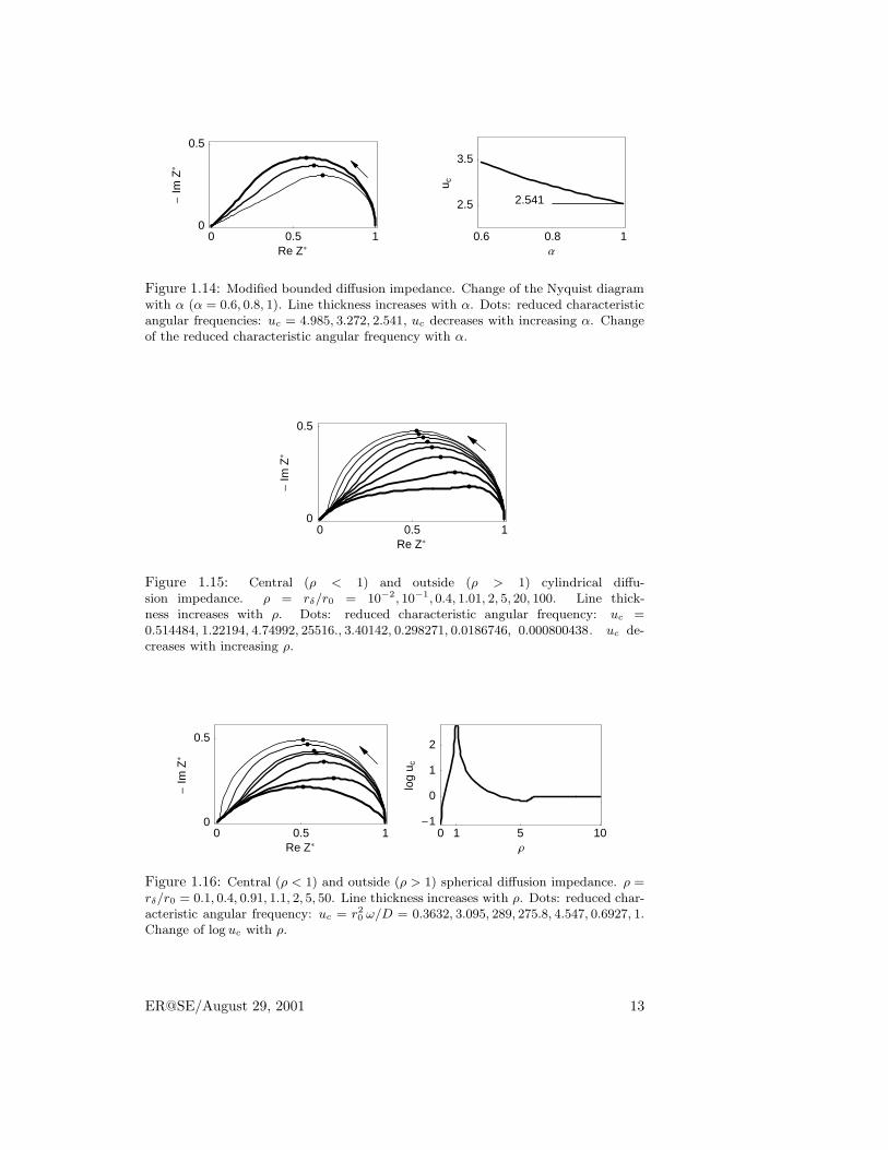
Figure 1.14: Modified bounded diffusion impedance. Change of the Nyquist diagramwith α (α = 0.6, 0.8, 1). Line thickness increases with α. Dots: reduced characteristicangular frequencies: uc = 4.985, 3.272, 2.541, uc decreases with increasing α. Changeof the reduced characteristic angular frequency with α.
0 0.5 1Re Z
0
0.5
Im
Z
Figure 1.15: Central (ρ < 1) and outside (ρ > 1) cylindrical diffu-sion impedance. ρ = rδ/r0 = 10−2, 10−1, 0.4, 1.01, 2, 5, 20, 100. Line thick-ness increases with ρ. Dots: reduced characteristic angular frequency: uc =0.514484, 1.22194, 4.74992, 25516., 3.40142, 0.298271, 0.0186746, 0.000800438. uc de-creases with increasing ρ.
0 0.5 1Re Z
0
0.5
Im
Z
0 1 5 10Ρ
1
0
1
2
log
u c
Figure 1.16: Central (ρ < 1) and outside (ρ > 1) spherical diffusion impedance. ρ =rδ/r0 = 0.1, 0.4, 0.91, 1.1, 2, 5, 50. Line thickness increases with ρ. Dots: reduced char-acteristic angular frequency: uc = r2
0 ω/D = 0.3632, 3.095, 289, 275.8, 4.547, 0.6927, 1.Change of log uc with ρ.
ER@SE/August 29, 2001 13

0 0.5 1Re Z
0
0.5
Im
Z
1 0 5 10∆
1
0
1
2
log
u clog 2.54
Figure 1.17: Central (δ < 0) and outside (δ > 0) spherical diffusion impedance.δ = (rδ − r0)/r0 = −0.99,−0.8,−0.5,−0.1, 0.1, 1, 3, 100. Line thickness in-creases with δ. Dots: reduced characteristic angular frequency: uc = (rδ −r0)
2 ω/D = 0.0299, 0.577, 1.37, 2.32, 2.76, 4.55, 8.33, 104fcylr0rdfcylr0rd, uc increaseswith δ. Change of log uc with δ.
ER@SE/August 29, 2001 14

Chapter 2
Gerischer anddiffusion-reactionimpedance
2.1 Gerischer and modified Gerischer impedance
2.1.1 Gerischer impedance
Z∗G(u) =
1√1 + iu
”In view of the earliest derivation of such an impedance by Gerischer, [4] itseems a good idea to name it the ”Gerischer impedance” ZG [15, 16].
0 0.5 1Re ZG
0
0.5
Im
ZG
uc
3
Figure 2.1: Reduced Gerischer impedance.
limu→0
Z∗G(u) = 1, lim
u→∞
√iuZ∗
G(u) = 1
Re Z∗G(u) =
cos(arctan(u)
2)
(1 + u2)1/4=
√√1 + u−2 + u−1
√2√1 + u−2
√u
Im Z∗G(u) = −
sin(arctan(u)
2)
(1 + u2)1/4= −
√√1 + u−2 − u−1
√2√1 + u−2
√u
15

dIm Z∗G(u)
du=
−2 +√1 + u−2 u
2√2√1 + u−2
√√1 + u−2 − 1
u
√u (1 + u2)
= 0 ⇒ uc =√3
2.1.2 Modified Gerischer impedance
Z∗Gα(u) =
1√1 + (iu)α
0 0.5 1Re ZGΑ
0
0.4
Im
ZGΑ
Figure 2.2: Reduced modified Gerischer impedance. α = 0.5, 0.6, 0.7, 0.8, 0.9, 1. Linethickness increases with α.
Re Z∗Gα(u) =
cos(12arctan(
uα sin(π α2 )
1 + uα cos(π α2 )
))
(1 + u2 α + 2 uα cos(π α
2 )) 1
4
Im Z∗Gα(u) = −
sin(12arctan(
uα sin(π α2 )
1 + uα cos(π α2 )
))
(1 + u2 α + 2 uα cos(π α
2 )) 1
4
0.5 0.75 1Α
2
3
u c
3
0.5 0.75 1Α
0
5
uc 3Αu
c%
Figure 2.3: Change of uc for modified Gerischer impedance (solid line) and change of√3/α with α (dashed line). uc ≈
√3/α for α ∈ [0.53, 1] (|(uc −
√3/α)|/uc < 5%).
2.2 Diffusion-reaction impedance
2.2.1 Reduced impedance #1
Z∗(u) =√λ coth
√λ tanh
√iu+ λ√
iu+ λ
ER@SE/August 29, 2001 16

limu→0
Z∗(u) = 1, limu→∞
√iu+ λZ∗(u) =
√λ coth
√λ
limλ→0
Z∗(u) = Z∗Wδ(u) =
tanh√iu√
iu, lim
λ→∞Z∗(u) = Z∗
G(u/λ) =1√
1 + u/λ
@verifier limite lorsque lambda tend vers l’infini
0 0.5 1Re Z
0
0.5
Im
Z
2 0 2log Λ
0
1
2
3
log
u c
log 2.541
Figure 2.4: Diffusion reaction reduced impedance #1. λ = 10−3, 1, 103. Line thick-ness increases with λ. uc = 2.542, 3.657, 1732. Change of log uc with log λ for diffusionreaction reduced impedance #1. λ → 0 ⇒ uc → 2.54, λ → ∞ ⇒ uc ≈ λ
√3.
Re Z∗(u) =
√λ coth(
√λ)(sinh(2
(u2 + λ2
) 14 cauλ) cauλ + sin(2
(u2 + λ2
) 14 sauλ) sauλ
)(u2 + λ2)
14
(cos(2 (u2 + λ2)
14 sauλ) + cosh(2 (u2 + λ2)
14 cauλ)
)
cauλ = cos(arctan(u
λ)2
), sauλ = sin(arctan(u
λ )2
)
Im Z∗(u) =
√λ coth(
√λ)(sin(2
(u2 + λ2
) 14 sauλ) cauλ − sinh(2
(u2 + λ2
) 14 cauλ) sauλ
)(u2 + λ2)
14
(cos(2 (u2 + λ2)
14 sauλ) + cosh(2 (u2 + λ2)
14 cauλ)
)
2.2.2 Reduced impedance #2
Z∗(u) =
√λ coth
√λ tanh
√(1 + iu) λ√
(1 + iu) λ
limu→0
Z∗(u) = 1, limu→∞
√(1 + iu)λZ∗(u) =
√λ coth
√λ
limλ→0
Z∗(u) = ZWδ(u/λ) =tanh
√iu/λ√
iu/λ, limλ→∞
Z∗(u) = Z∗G(u) =
1√1 + iu
Re Z∗(u) =coth(
√λ)(sinh(2
(1 + u2
) 14√λ cau) cau + sin(2
(1 + u2
) 14√λ sau) sau
)(1 + u2)
14
(cos(2 (1 + u2)
14√λ sau) + cosh(2 (1 + u2)
14√λ cau)
)
cau = cos(arctan(u)
2), sau = sin(
arctan(u)2
)
Im Z∗(u) =coth(
√λ)(sin(2
(1 + u2
) 14√λ sau) cau − sinh(2
(1 + u2
) 14√λ cau) sau
)(1 + u2)
14
(cos(2 (1 + u2)
14√λ sau) + cosh(2 (1 + u2)
14√λ cau)
)
ER@SE/August 29, 2001 17

0 0.5 1Re Z
0
0.5
Im
Z
2 0 2log Λ
0
1
2
3
log
u c
log
3
Figure 2.5: Diffusion reaction reduced impedance #2. λ = 10−4, 1, 103. Line thick-ness increases with λ. uc = 25407, 3.657, 1.732. Change of log uc with log λ for diffusionreaction reduced impedance #1. λ → 0 ⇒ uc ≈ 1/(2.54 λ), λ → ∞ ⇒ uc →
√3.
2.3 Appendix
@ infinite outside cylindrical
ER@SE/August 29, 2001 18

Symbol Name Reduced impedance Impedance diagram
ZW Warburg1√iu
0 1Re ZW
0
1
Im
ZW
u1
ZG Gerischer1√
1 + iu0 0.5 1
Re ZG
0
0.5
Im
ZG
uc
3
ZGα Modified Gerischer1√
1 + (iu)α0 0.5 1
Re ZGΑ
0
0.4
Im
ZGΑ
uc
3 Α
semi-∞ spherical diffusion1
1 +√iu 0 0.5 1
Re Z
0
0.2
Im
Z uc1
ZWδBounded diffusion
tanh√iu√
iu0 0.5 1
Re ZW∆
0
0.5
Im
ZW∆
uc2.541
ER@SE/August 29, 2001 19

ER@SE/August 29, 2001 20

Bibliography
[1] Armstrong, R. D., Bell, M. F., and Metcalfe, A. A. The A.
C. impedance of complex electrcochemical reactions. In Electrochemistry,vol. 6. The Chemical Society, Burlington House, London, 1978, ch. 3,pp. 98–127.
[2] Barral, G., Diard, J.-P., and Montella, C. etude d’un modelede reaction electrochimique d’insertion. I-Resolution pour une commandedynamique a petit signal. Electrochim. Acta 29 (1984), 239–246.
[3] Drossbach, P., and Schultz, J. Electrochim. Acta 11 (1964), 1391.
[4] Gerischer, H. Z. Physik. Chem. (Leipzig) 198 (1951), 286.
[5] Jacobsen, T., and West, K. Diffusion impedance in planar cylindricaland spherical symmetry. Electrochim. Acta 40 (1995), 255–262.
[6] Lasia, A. Electrochemical Impedance Spectroscopy and its Applications.In Modern Aspects of Electrochemistry, vol. 32. Kluwer Academic/PlenumPublishers, 1999, ch. 2, pp. 143–248.
[7] Llopis, J., and Colon, F. In Proceedings of the Eighth Meeting of theC.I.T.C.E. (London, 1958), C.I.T.C.E., Butterworths, p. 144.
[8] Macdonald, J. R. Impedance spectroscopy. Emphasing solid materialsand systems. John Wiley & Sons, 1987.
[9] Mahon, P. J., and Oldham, K. B. Convolutive modelling of electro-chemical processes based on the relationship between the current and thesurface concentration. J. Electroanal. Chem. 464 (1999), 1–13.
[10] Mohamedi, M., Bouteillon, J., and Poignet, J.-C. Electrochemicalimpedance spectroscopy study of indium couples in LiCl-KCl eutectic at450C. Electrochim. Acta 41 (1996), 1495–1504.
[11] Montella, C. EIS study of hydrogen insertion under restricted diffu-sion conditions. I. Two-step insertion reaction. J. Electroanal. Chem. 497(2001), 3–17.
[12] Randles, J. E. Discuss. Faraday Soc. 1 (1947), 11. 1947, a great yearfor equivalent circuits, wine (in France) and men (in France).
[13] Schuhmann, D. Compt. rend. 262 (1966), 1125.
21

[14] Sluyters, J. H. PhD thesis, Utrecht, 1956.
[15] Sluyters-Rehbach, M. Impedance of electrochemical systems:terminology, nomenclature and representation-part i: cells with metal elec-trodes and liqui solution (IUPAC Recommendations 1994). Pure & Appl.Chem. 66 (1994), 11831–1891.
[16] Sluyters-Rehbach, M., and Sluyters, J. H. In Comprehensive Trea-tise of Electrochemistry, B. C. E. Yeager, J. O’M Bockris and S. S. Eds.,Eds., vol. 9. Plenum Press, New York and London, 19??, p. 274.
[17] Sluyters-Rehbach, M., and Sluyters, J. H. Sine wave methods inthe study of electrode processes. In Electroanalytical Chemistry, A. J. Bard,Ed., vol. 4. Marcel Dekker, Inc;, New York, 1970, ch. 1, pp. 1–128.
[18] VanderNoot, T. J. Limitations in the analysis of ac impedance datawith poorly separated faradaic and diffusional processes. J. Electroanal.Chem. 300 (1991), 199–210.
[19] Warburg, E. Uber das Verhalten sogenannter unpolarisierbarerElectroden gegen Wechselstrom. Ann. Phys. Chem. 67 (1899), 493–499.
[20] Wolfram, S. Mathematica Version 3. Cambridge University Press, 1996.
[21] Yzermans, A. B. PhD thesis, Utrecht, 1965.
ER@SE/August 29, 2001 22


