

EXPERIMENTAL STUDY OF A TWO-DOF FIVE
BAR CLOSE-LOOP MECHANISM
A Thesis Submitted to the
College of Graduate Studies and Research
In Partial Fulfillment of the Requirements
for the Degree of Master of Science
in The Department of Mechanical Engineering
University of Saskatchewan
Canada
By
Reza Moazed
©Copyright R. Moazed, August 2006. All rights reserved.

i
PERMISSION TO USE
In presenting this thesis in partial fulfillment of the requirements for a Postgraduate
degree from the University of Saskatchewan, I agree that the Libraries of this University
may make it freely available for inspection. I further agree that permission for copying of
this thesis in any manner, in whole or in part, for scholarly purposes may be granted by
the professor or professors who supervised my thesis work or, in their absence, by the
Head of the Department or the Dean of the College in which this thesis was done. It is
understood that any copying or publication or use of this thesis or parts thereof for
financial gain shall not be allowed without my written permission. It is also understood
that due recognition shall be given to me and to the University of Saskatchewan in any
scholarly use which may be made of any material in my thesis.
Requests for permission to copy or to make other use of material in this thesis in whole or
part should be addressed to:
Head of the Department of Mechanical Engineering
University of Saskatchewan
Saskatoon, Saskatchewan
Canada S7N 5A9

ii
ABSTRACT
This research is to carry out an experimental study to examine and verify the
effectiveness of the control algorithms and strategies developed at the Advanced
Engineering Design Laboratory (AEDL). For this purpose, two objectives are set to be
achieved in this research. The first objective is to develop a generic experiment
environment (test bed) such that different control approaches and algorithms can be
implemented on it. The second objective is to conduct an experimental study on the
examined control algorithms, as applied to the above test bed.
To achieve the first objective, two main test beds, namely, the real-time controllable
(RTC) mechanism and the hybrid machine, have been developed based on a two degree
of freedom (DOF) closed-loop five-bar linkage. The 2-DOF closed-loop mechanism is
employed in this study as it is the simplest of multi-DOF closed-loop mechanisms, and
control approaches and conclusions based on a 2-DOF mechanism are generic and can be
applied to a closed-loop mechanism with a higher number of degrees of freedom. The
RTC mechanism test bed is driven by two servomotors and the hybrid machine is driven
by one servomotor and a traditional CV motor.
To achieve the second objective, an experimental study on different control algorithms
has been conducted. The Proportional Derivative (PD) based control laws, i.e., traditional

iii
PD control, Nonlinear-PD (NPD) control, Evolutionary PD (EPD) control, non-linear PD
learning control (NPD-LC) and Adaptive Evolutionary Switching-PD (AES-PD) are
applied to the RTC mechanism; and as applied to the Hybrid Actuation System (HAS),
the traditional PD control and the SMC control techniques are examined and compared.
In the case of the RTC mechanism, the experiments on the five PD-based control
algorithms, i.e., PD control, NPD control, EPD, NPD-LC, and AES-PD, show that the
NPD controller has better performance than the PD controller in terms of the reduction in
position tracking errors. It is also illustrated by the experiments that iteration learning
control (ILC) techniques can be used to improve the trajectory tracking performance.
However, AES-PD showed to have a faster convergence rate than the other ILC control
laws. Experimental results also show that feedback ILC is more effective than the
feedforward ILC and has a faster convergence rate. In addition, the results of the
comparative study of the traditional PD and the Computed Torque Control (CTC)
technique at both low and high speeds show that at lower speeds, both of these controllers
provide similar results. However, with an increase in speed, the position tracking errors
using the CTC control approach become larger than that of the traditional PD control.
In the case of the hybrid machine, PD control and SMC control are applied to the
mechanism. The results show that for the control of the hybrid machine and the range of
speed used in this experimental study, PD control can result in satisfactory performance.
However, SMC proved to be more effective than PD control.

iv
ACKNOWLEGMENTS
I would like to take this opportunity to express my sincere thanks to my supervisors,
Professor C. Zhang and Professor D. Chen, for their valuable guidance and continuous
encouragement in the whole research as well as the critical review of the manuscript.
I would like to extend my special thanks to the other members of my advisory committee:
Professor M. M. Gupta, Professor R. Fotouhi for their valuable support and constructive
suggestions throughout the course of this project.
I also acknowledge Dr. P. Ouyang, a former graduate student at the AEDL for his
valuable suggestions and advice. I would also like to thank Mr. R.J. Wilson for making
the HAS prototype used in this experimental study, and Mr. D. Bitner for his help with
the experimental set-up of the RTC mechanism.

v
Dedicated to my mom and dad
Dr. Hadi Moazed and MRS. Malikeh Jafar Nejadi

vi
Table of Contents
PERMISSION TO USE………………………………………………………….……….i
ABSTRACT………...…………………………………………………………………….ii
ACKNOWLEDGMENTS………………………………………………………………..iv
TABLE OF CONTENTS…………………………………………………………….......vi
LIST OF TABLES………………………………………………………………………...x
LIST OF FIGURES………………………………………………………………………xi
ACRONYMS…………………………...……………………………………………….xiv
CHAPTER 1 Introduction………………………………1
1.1 Background and motivation…………………………………………………………...1
1.2 Traditional Mechanisms Vs Mechatronic Mechanisms……………………………….3
1.3 Research objectives and scopes……………………………………………………….5
1.4 General Methodology…………………………………………………………………6
1.5 Organization of the thesis……………………………………………………………..8
CHAPTER 2 Literature Review………………………10
2.1 Introduction…………………………………………………………………………..10
2.2 Servo mechanisms and hybrid actuation systems…………………………………....11
2.3 Dynamics of multi-DOF closed-loop mechanisms…………………………………..13
2.4 Control Schemes for Multi-DOF Closed-loop Mechanisms………………………...22
2.4.1 PD based control methods………………………………………………....22
vii
2.4.2 Model based control methods……………………………………………...24
2.5 Previous works developed at the AEDL at the University of Saskatchewan………..25
2.6 Trajectory planning methods………………………………………………………...26
2.7 Summary……………………………………………………………………………..27
CHAPTER 3 Test Beds for Experimental Study
3.1 Introduction…………………………………………………………………………..28
3.2 Two DOF Five Bar Linkage Close-loop Mechanism………………………………..29
3.3 RTC mechanism test bed…………………………………………………………….33
3.4 Hybrid Actuation system test bed……………………………………………………36
3.5 User interface of the test beds………………………………………………………..40
3.6 Position and Velocity measurements………………………………………………...42
3.7 Summary……………………………………………………………………………..43
CHAPTER 4 Control Algorithms……………………..44
4.1 Introduction…………………………………………………………………………..44
4.2 PD and NPD control laws……………………………………………………………45
4.3 Iteration Learning Control (ILC)…………………………………………………….47
4.3.1 Iterative learning…………………………………………………………...47
4.3.2 Evolutionary PD (EPD) control law……………………………………….49
4.3.3 Adaptive Evolutionary Switch Gain PD Control (AES-PD)………………50
4.3.4 Adaptive Nonlinear PD learning control (NPD-LC)………………………52

viii
4.4 Computed Torque Control (CTC) algorithm………………………………………...53
4.5 Summary and Discussion…………………………………………………………….54
CHAPTER 5 EXPERIMENTS AND RESULTS ON THE RTC MECHANISM……………...56
5.1 Introduction…………………………………………………………………………..56
5.2 Trajectory planning for the two servomotors………………………………………...57
5.3 PD and NPD control laws……………………………………………………………59
5.4 EPD control law……………………………………………………………………...65
5.5 NPD-LC control law…………………………………………………………………71
5.6 AES-PD control law…………………………………………………………………76
5.7 Comparison of the PD, NPD, EPD, AES-PD, NPD-LC Control methods…………..82
5.8 Comparison of Feedforward ILC control to Feedback ILC control…………………86
5.9 Comparison of CTC control law to PD control law…………………………………89
5.10 Comments on the experiment………………………………………………………92
5.10.1 Initial position error………………………………………………………92
5.10.2 Sampling period…………………………………………………………..93
5.10.3 Estimations of velocity…………………………………………………...93
5.11 Conclusion………………………………………………………………………….94
CHAPTER 6 EXPERIMENTS AND RESULTS ON THE HAS MECHANISM……………...96
6.1 Introduction…………………………………………………………………………..96

ix
6.2 Dynamic model of the hybrid actuation system……………………………………..97
6.3 Sliding Mode Control (SMC) for nonlinear systems……………………………….100
6.4 Trajectory Planning for the CV and Servomotor…………………………………...104
6.5 Experimental Results of the HAS…………………………………………………..105
6.7 Conclusion………………………………………………………………………….113
Chapter 7 Conclusion and Recommendation………..114
7.1 Overview of the thesis……………………………………………………………...114
7.2 Major Conclusions………………………………………………………………….115
7.3 Future Work………………………………………………………………………...116
References……………………………………………...118

x
LIST OF TABLES
Table 3.1 Parameters of the five-bar mechanism………………………………………...31
Table 5.1 Performance improvement with the EPD control at the low speed case……...69
Table 5.2 Performance improvement with the EPD control at the high speed case……..70
Table 5.3 Performance improvement with the NPD-LC control at the low speed case…75
Table 5.4 Performance improvement with the NPD-LC control at the high speed case ……………………………………………………………………………………………75 Table 5.5 Performance improvement with the AES-PD control at the low speed case….80
Table 5.6 Performance improvement with the AES-PD control at the high speed case ……………………………………………………………………………………………80 Table 5.7: Experimental Results for PD, NPD, EPD, NPD-LC, AES-PD at the low speed case (maximum errors and torques in the actuators)…………………………………….80 Table 5.8: Experimental Results for PD, NPD, EPD, NPD-LC, AES-PD at the high speed case (maximum errors and torques in the actuators)…………………………………….85 Table 5.9 Performance improvement comparison of feedforward ILC and feedback ILC ………………………………………………………………………………………88 Table 6.1 The parameters of the two motors…………………………………………...107

xi
LIST OF FIGURES
Figure 2.1: The structure of a 2 DOF parallel robot……………………………………..15
Figure 3.1: Five-bar linkage mechanism………………………………………………...29
Figure 3.2: Schematic of a five-bar linkage mechanism (Ouyang, 2002)……………….30
Figure 3.3: Individual links of the five-bar mechanism: (a) Link 1, (b) Link 2, (c)Link 3, and (d) Link 4…………………………………………………………………………….31 Figure 3.4: RTC mechanism test bed…………………………………………………….34
Figure 3.5: Control diagram of the RTC mechanism……………………………………35
Figure 3.6: Hybrid actuation system test bed…………………………………………….37
Figure 3.7: Control diagram of the HAS mechanism……………………………………38
Figure 3.8: User Interface developed in C++ in the case of the RTC mechanism………..40
Figure 4.1: Iterative scheme of the iteration learning control algorithm………………...48
Figure 5.1: Experimental results by applying PD and NPD controllers for the low speed case: (a) angle error of Actuator 1 and (b) angle error of Actuator 2……………………61 Figure 5.2: Experimental results by applying PD and NPD controllers for the low speed case: (a) torque of Actuator 1 and (2) torque of Actuator 2……………………………...62 Figure 5.3: Experimental results by applying PD and NPD controllers for the high speed case: (a) angle error of Actuator 1 and (b) angle error of Actuator 2……………………63 Figure 5.4: Experimental results by applying PD and NPD controllers for the high speed case: (a) torque of Actuator 1 and (2) torque of Actuator 2……………………………...64 Figure 5.5: Experimental results by applying EPD controller for the low speed case (Iterations 1 to 3): (a) angle error of Actuator 1 and (b) angle error of Actuator 2……..67

xii
Figure 5.6: Experimental results by applying EPD controller for the low speed case (Iterations 3 to 6): (a) angle error of Actuator 1 and (b) angle error of Actuator 2……..68 Figure 5.7: Experimental results by applying EPD controller for the high case (Iterations 1 to 4): (a) angle error of Actuator 1 and (b) angle error of Actuator 2…………………69 Figure 5.8: Experimental results by applying NPD-LC controller for the low speed case (Iterations 1 to 3): (a) angle error of Actuator 1 and (b) angle error of Actuator 2……..72 Figure 5.9: Experimental results by applying NPD-LC controller for the low speed case (Iterations 3 to 6): (a) angle error of Actuator 1 and (b) angle error of Actuator 2……..73 Figure 5.10: Experimental results by applying NPD-LC controller for the high speed case (Iterations 1 to 4): (a) angle error of Actuator 1 and (b) angle error of Actuator 2……..74 Figure 5.11: Experimental results by applying AES-PD controller for the low speed case (Iterations 1 to 3): (a) angle error of Actuator 1 and (b) angle error of Actuator 2……..77 Figure 5.12: Experimental results by applying AES-PD controller for the low speed case (Iterations 3 to 6): (a) angle error of Actuator 1 and (b) angle error of Actuator 2……..78 Figure 5.13: Experimental results by applying AES-PD controller for the high speed case (Iterations 1 to 4): (a) angle error of Actuator 1 and (b) angle error of Actuator 2……..79 Figure 5.14 Comparison of the trajectory tracking performance with PD-based controllers at the low speed case: (a) angle error of Actuator 1 and (b) angle error of Actuator 2….83 Figure 5.15 Comparison of the trajectory tracking performance with PD-based controllers at the high speed case: (a) angle error of Actuator 1 and (b) angle error of Actuator 2…84 Figure 5.16: Experimental results by applying Feedforward ILC for the low speed case (Iterations 1 to 6): (a) angle error of Actuator 1 and (b) angle error of Actuator 2……..88 Figure 5.17: Experimental results by applying CTC and PD control for the low speed case: (a) angle error of Actuator 1 and (b) angle error of Actuator 2…………………...90 Figure 5.18: Experimental results by applying CTC and PD control for the high speed case: (a) angle error of Actuator 1 and (b) angle error of Actuator 2…………………...91 Figure 6.1: Measured position tracking errors in the motors for the low speed case using PD controller: (a) angle error of Servomotor and (b) angle error of CV motor……….108 Figure 6.2: Measured position tracking errors in the motors for the high speed case using PD controller: (a) angle error of Servomotor and (b) angle error of CV motor……….109

xiii
Figure 6.3: Measured position tracking errors in the motors for the low speed case using SMC: (a) angle error of Servomotor and (b) angle error of CV motor…………………110 Figure 6.4: Measured position tracking errors in the motors for the high speed case using SMC: (a) angle error of Servomotor and (b) angle error of CV motor…………………111

xiv
ACRONYMS
AEDL Advanced engineering design laboratory
CTC Computed torque control
DOF Degree of freedom
EPD Evolutionary PD
NPD Nonlinear PD
PD Proportional derivative
RTC Real-time controllable
CV constant velocity
SMC sliding mode control
ILC Iteration learning control
NPD-LC nonlinear-PD learning control
AES-PD Adaptive evolutionary switching PD control
HAS Hybrid actuation system

1
Chapter 1 Introduction 1.1 Background and motivation Mechanisms can be classified into two main categories based on their structures, namely,
serial and parallel. A serial type mechanism has its links sequentially connected,
constructing an open loop. In general, the first link of the open chain structure originates
from a fixed base and it is subsequently connected to the other links with the last one
having an open end. The end effector is usually mounted to the last link. In contrast with
the open loop structure, the end effector of a close-loop mechanism is linked to the fixed
base by the use of multiple kinematic chains. Normally all the actuators of these
mechanisms are located on or close to the base (Li and Wu, 2004). Closed-loop structure
mechanisms are also sometimes referred to as parallel mechanisms in the literature.
Serial type structures have some inherent disadvantages such as low position accuracy
and mechanical stiffness. For instance, the position accuracy of a serial mechanism with
many links is considerably low, since a small amount of error at each joint is enlarged

2
and accumulated by its subsequent links (Li et al., 2000). As well, the mechanical
stiffness of the open-loop structure is essentially poor considering that each link has to
carry the mass of its subsequent links and their actuators. In comparison to their serial
counterparts, parallel structures have a high stiffness, high motion accuracy and high
load-structure ratio. Due to their advantages over serial structure mechanisms, parallel
structure mechanisms have been receiving increasing interest from both academia and
industries in recent years.
To obtain the same number of degrees of freedom (DOF), a closed-loop structure is far
more complex than an open-loop one, thereby resulting in a more complex dynamic
model in general. It is common knowledge in the field of controls that for the control of a
mechanism with a more complex dynamics a more sophisticated control algorithm is
usually required. Therefore, it is clear that for the control of a parallel mechanism a more
advanced control algorithm is necessary in comparison to the serial structure mechanism.
Due to the complexity of the dynamic model of parallel mechanisms, the control of these
structures is a challenging and difficult task. Numerous control algorithms and methods
are proposed for the control of these structures, including several control algorithms that
have been developed for the control of parallel mechanisms throughout the years in the
Advanced Engineering Design Laboratory (AEDL) at the University of Saskatchewan.
The need of research to generalize these developments and to develop experimental
means in conjunction with the theoretical work is the main motivating factor behind this
study.

3
This study will focus on the experimental work to verify the theoretical works recently
completed in the AEDL. In particular, the test bed developed for the experimental study,
which consists of a 2 degree of freedom (DOF) parallel mechanism will be described; as
well the results of the experiments conducted will be presented and discussed in order to
illustrate and validate the effectiveness of the different control algorithms previously
developed at the AEDL.
1.2 Traditional Mechanisms Vs Mechatronic Mechanisms According to the International Federation for the Promotion of Mechanism and Machine
Science (IFToMM), a mechanism is defined as a set of connected components to perform
a definite motion and force transfer (IFToMM, 1991). Traditionally, a mechanism is
viewed as a structure that has at least one DOF and is driven by one or more constant
velocity motors. These motors are not real-time controllable (RTC) or adjustable and
such a traditional mechanism is termed a non-RTC mechanism.
If a mechanism is driven by real-time controllable (RTC) motors or servomotors, then it
is called an RTC mechanism. Due to the use of servomotors, the RTC mechansim can be
planned and programmed in real-time. RTC mechanisms are also called mechatronic
mechanisms in the literature and in general are multi-degrees of freedom systems. There
are many advantages associated with the use of servomotors in machines as the
mechanism can be used for more diversified purposes due to its programmablitliy.
Robotic applications in which a manipulator produces flexible motions under various
payloads is a good example of this concept (Ouyang, 2002).

4
RTC motors are used in many advanced robots and machine tools. This is due to their
real time controllability which enables them to adapt to different applications without the
need to redesign the mechanical structure of the mechanism. One of the typical
applications of RTC mechanisms is to track motion, in which a trajectory of the end-
effector is desired and given as a function of time and then the mechanism is controlled
such that the end-effector follows the given trajectory. Another typical application of
RTC mechanisms is to track a set of points, in which the motion between any two points
is not of interest. The point-set tracking problem can be viewed as a simplified version of
the trajectory tracking problem, so tracking of a trajectory is generally more demanding
than tracking of a set of points. This thesis concentrates on trajectory tracking. Although
RTC motors can be programmed to follow a desired trajectory, it is important to note that
in the case of non-RTC mechanisms, trajectory generation is a generic design problem.
This problem, however, does not usually involve the time factor, and nor is the feedback
control involved (Klein, 1987; Ouyang, 2002).
It is possible for a mechanism to incorporate both RTC and non-RTC motors for its drive.
In this thesis, a mechanical system where its drive includes two types of motors, a
servomotor and a constant velocity (CV) motor, is referred to as the hybrid actuation
system. Hybrid actuation systems provide a middle ground between the traditional
inflexible machines and the modern flexible robots. These systems will be discussed in
more details in the following chapters.

5
1.3 Research objectives and scopes The research presented in this thesis focuses on experimentally verifying some of the
control algorithms and approaches developed at the AEDL as well as reported in the
literature. In particular, the following research objectives are set to be achieved.
Objective 1: Develop a generic experiment environment (test bed) such that different
control approaches and algorithms can be implemented on it.
It is remarked that a 2 DOF mechanism is used as a generic experiment environment. The
term generic here is used since the 2 DOF closed loop mechanism is the simplest of
multi-DOF closed loop systems and the approaches, methods and conclusions based on a
2 DOF mechanism can all be applied to a structure with a higher number of degrees of
freedom (Wang, 2000).
It is also remarked that the 2 DOF closed loop mechanism is studied under two different
experimental setups. In the first case, the mechanism is driven by two RTC motors (i.e.,
servomotors) and therefore is real time controllable. In the second case, the mechanism is
a hybrid actuation system and is driven by a traditional non-RTC constant speed motor
and a servo motor. It is noted that existing research on hybrid actuation systems usually
employs two servomotors, one of which is used to mimics the behavior of a constant
velocity motor. It is obvious that this is different than the real situation where a CV motor
is in place. This study differs from existing ones in that a CV motor and a servomotor are
used for the hybrid actuation system.

6
Objective 2: Conduct an experimental study on different control algorithms,
including error-based control algorithms, such as proportional derivative (PD), non-
linear PD (NPD), iterative learning methods (ILC), and model-based control
algorithms such as computed torque control (CTC) and Sliding Mode Control (SMC),
as applied to the above test beds.
It is remarked that in this thesis, model based control refers to those control approaches in
which the dynamic model of the plant is employed into their control law. In comparison,
error based control methods refer to those control approaches that are based just on the
errors of the system and do not take the dynamic model of the plant into consideration. At
high speeds, the calculation of the dynamic model poses a challenge due to its heavy
computational time. Therefore, model based control approaches might not result in
satisfactory performance at higher speeds.
To measure the performance trajectory tracking, two indices are used in this study, i.e., (i)
the error between the predefined motion and the actual one and (ii) the peak driving
torque required from the servo motors.
1.4 General Methodology
To achieve Objective 1, a five-bar (closed loop) mechanism with two degrees-of-freedom
is to be designed and developed. The five-bar mechanism has a wide range of

7
applications and its motion control has been intensively investigated (Youcef-Toumi and
Kuo, 1993; Guo et al., 1999; Ghorbel, 1995). It should be noted that the five-bar
mechanism is the typical structure of multi-DOF and closed-loop mechanical systems,
and the results obtained from it would be of generalized implications (Wang, 2000).
It should be noted that with respect to objective 1, two different experimental setups are
developed. The first case is an RTC mechanism driven by two servomotors which is used
to test the effectiveness of different control methods such as the traditional PD control,
NPD control, ILC iterative control techniques and the well known CTC control strategy.
For the second case, a CV motor and a servomotor are used to develop a hybrid actuation
system. This prototype is to be employed to carry out an experimental study of hybrid
actuation machines. A control method known as the sliding mode control will be
implemented on the system. The prototype developed and the results of the experiments
conducted will be discussed in chapters 3 and 5 respectively.
To achieve Objective 2, the generic experiment environment developed will be used to
conduct experiments in order to verify the effectiveness and validity of the control
algorithms mentioned in the objective. Experiments are conducted to test the
effectiveness of the ILC learning control methods proposed at the AEDL. ILC control
used in the previous literature is feedforward or off-line learning control. In this type of
iterative learning control, information for computing the current torque profile does not
come from the present iteration, but from the previous one. ILC control proposed at the
AEDL, however, is an online learning control in that the controlled torque of the current

8
iteration consists of a combination of the current controlled torque (feedback) and also
the torque profile produced in the previous iteration (feedforward). It is expected that the
latter type of ILC control provides more satisfactory results since its torque profile is a
combination of the current and previous iterations. Experiments are conducted to see the
effectiveness of feedforward and feedback ILC and the results are presented in Chapter 5.
It is remarked that for the control of a complex mechanical structure for precise and fast
performance, an advanced controller based on an accurate system dynamic model is
usually desired. In the case of controlling parallel robots, however, the intensive
computation due to the complexity of the dynamic model can result in difficulties in the
physical implementation of the controllers for high-speed performance. Therefore more
complex control methods, such as model based control approaches might not yield
satisfactory results at higher speeds due to heavy computational time. In chapter 5, the
traditional PD control law (i.e., error based control) is compared to the CTC control law
(i.e., model based control) at low and high speeds, to get a measure of the effectiveness of
error based and model based control algorithms at these two operating conditions.
1.5 Organization of the thesis
This thesis consists of seven chapters. In chapter 2, a literature review of the dynamics
and control of the 2 DOF five-bar closed loop mechanism is presented, with a goal to
further analyze and justify the objectives of this thesis.

9
Chapter 3 presents the design and development of the test beds for experiments. In
particular, motor, amplifier, servo drive and controller configuration and specifications
will be discussed in detail; and the design of the test beds will be presented.
In Chapter 4, different control approaches examined in this study will be reviewed and
outlined. These control approaches include proportional derivative (PD), non-linear PD
(NPD), iterative learning methods (ILC), and computed torque control (CTC).
In chapter 5, the results of the experiments conducted on the RTC mechanism will be
presented and analyzed.
In chapter 6, the hybrid actuation system is considered and discussed in details. As well,
sliding mode control for the control of hybrid actuation systems will also be introduced.
The results of the experiments conducted using the hybrid machine test bed and applying
sliding mode control are also presented and discussed in this chapter.
Chapter 7 presents the conclusions drawn from this research, which is followed by
suggestions and recommendations for possible future work.

10
Chapter 2 Literature Review 2.1 Introduction This chapter is to provide a brief review of past and recent developments in the design,
modeling, and control of servo and hybrid mechanisms. The objective is to examine
various approaches that have been developed in this research topic and to identify the
issues involved, thereby justifying the necessity of the present research. Particularly, in
Section 2.2 servo mechanisms and hybrid actuation systems are discussed in detail, and
compared to identify their advantages and disadvantages. In Section 2.3, a dynamic
model of the 2 DOF closed loop mechanism used in this study is introduced and outlined.
In Section 2.4, two types of control which are of interest in this study, i.e., error based
and model based control schemes, are introduced. Section 2.5 presents the previous
relevant works that have been developed at the AEDL. This is followed by section 2.6,
discussing commonly-used approaches for trajectory tracking.

11
2.2 Servo mechanisms and hybrid actuation systems
A machine that is driven by two types of motors, namely, the servomotor and the
constant speed motor is called a hybrid machine. The advantage of this kind of machines
is their high reliability and power. In contrast, machines driven by only constant speed
motors suffer from the lack of task flexibility. Since all motions of non-RTC machines
are recognized in the hardware of the system (as they are not controllable and therefore
lack a control mechanism and a controller), an expensive and time consuming
reconstruction of the hardware is necessary for any modification to the motion of these
machines.
In comparison to the traditional mechanism, machines driven by servomotors are flexible
in operation by reprogramming of the servomotor. For servo mechanisms to achieve and
fulfill new task requirements, only the control program needs to be modified. For this
reason, these types of machines are often referred to as programmable machines in the
literature (Ouyang, 2004). Applications of such machines can be found in packaging
machinery, stamping, and machine tools.
The use of servomotors in machines has also drawbacks. One of these drawbacks is the
low ratio of the payload to the motor power capacity. Also, these machines provide poor
motion precision under high-speed operations. Servomotor-driven mechanisms operate in
a wide range of motion, which may include an extreme acceleration profile. This imposes

12
severe torque requirements on the motors, producing excessive torque variations that will
most likely create significant heat in the motor windings. Certain motor specifications
also constrain the range and speed of reachable output motions. Such characteristics
include the motor’s rated torque and peak power capability (Ouyang, 2002; Li and Wu,
2004). The use of servomotors in combination with the traditional constant speed motors
in closed loop mechanisms can alleviate these problems. The structure of a closed loop
mechanisms allows for the concept of hybrid machine which combines the power of the
traditional non-RTC motors with the programming and real time controllability of
today’s modern servomotors.
A few researchers have worked on the hybrid machine systems. Greenough et al (1995)
developed a hybrid machine system, which consists of a CV motor, a flywheel, and a
servomotor to construct a closed loop 2-DOF mechanism. The mechanism is driven by
the servomotor and the constant speed motor, both of which drive a single output and are
coupled through a 2-DOF mechanism. While the two motors drive the two independent
shafts supplying power to an output member, the trajectory of the servomotor is
controlled with a user specified motion and the CV motor is uncontrollable. In hybrid
machines, the CV motor supplies the mechanism with the majority of the power while the
servomotor acts as a driver providing low modulating torque.
Hybrid machines can also be a combination of several motors and mechanisms. Due to
the lower cost of CV motors in comparison to their servomotor counterparts as well as
their capability of energy recuperation, the use of hybrid machines makes it possible to

13
significantly reduce the operating cost (Tokuz and Jones, 1991; Tokuz 1992; Van de
Straete and De Schutter, 1996).
2.3 Dynamics of multi-DOF closed-loop mechanisms
In order to develop an effective controller for optimal trajectory tracking performance,
the dynamics of a mechanism must first be thoroughly analyzed. In this section the
dynamic model that describes the dynamical behavior of the 2-DOF closed loop
mechanism is introduced. The development of an accurate dynamic model plays a
significant role in the control of a mechanism in several ways. First, a precise dynamic
model is required to predict how a mechanism will react in response to the forces and
torques acting on it. Second, an accurate dynamic model is necessary for the development
of suitable control strategies.
Numerous methods and approaches have been developed in previous works for deriving
the dynamic equations of a mechanism (Thomson, 1993; Codourey, 1998; Ghorbel, 1994
and 1997). Newtonian mechanics and Lagrange’s method are the two most widely used
approaches to derive the dynamic model of mechanisms. The superiority of one approach
over another is solely based on the accuracy and computational efficiency of the model.
Whilst there has been numerous studies on the dynamic modeling of serial structures, but
little work has been done on modeling of parallel mechanisms. (Fitcher, 1986; Raghavan
et al., 1989; Reboulet et al., 1991; Liu et al., 1993; Ghorbel, 1994 and 1997; Gautier et al.,

14
1995; Ghorbel and Srinivasan, 1998). The difficulty in the dynamic modeling of closed-
loop mechanisms is due to the fact that some dependant joints are highly coupled with the
independent joint variables. Hall (1981) developed the dynamic model for a four bar,
single-DOF closed-loop mechanism using Lagrange’s equations of motion. Nguyen and
Cipra (1999) and Wang (2000) developed the dynamic model of a 2 DOF closed loop
planar mechanism following the same approach as in Hall (1981).
Reduced order model analysis method proposed by Ghorbel (1994, 1997) and modified
by Ouyang (2002) is another approach for the dynamic modeling of closed loop
mechanisms. This approach is described in full details in the remainder of this section
and is used to develop the dynamic model of the 2-DOF five-bar closed loop mechanism
used in this study. Ghorbel originally developed the dynamic model of a closed loop 2-
DOF mechanism using the reduced order model method, however, in his study the mass
centers are in-line with the link, meaning the center of mass of each link lies on the axis
of the link, i.e., iδ =0 in Figure 2.1. Ouyang (2002) extended Ghorbel’s method to a more
general situation, with off-line link mass centers. In Ouyang’s study the mass center of
each link in the mechanism is arbitrarily distributed with respect to the link’s reference
coordinate system (see Figure 2.1). The dynamic model developed by Ouyang (2002) is
adopted and used in this study. The development of the model is outlined as follows.
Consider a 2 DOF parallel robot shown in Figure 2.1. im is the mass of the individual
linkages, ir is the distance to the center of mass from the joint of link i , iL is the length
of link i , and iI is the inertia of link i . As mentioned previously, the center of mass of

15
each link is assumed to be offline with an angle iδ for the more general application. The
motion of the 2-DOF closed loop mechanism is governed by Ghorbel 1994, 1997 and
Ouyang, 2002.
Figure 2.1: The structure of a 2 DOF parallel robot
)()(
)(),()(
qqqqq
qgqqqCqqD
σρ
τ
=′′=′
=′+′′+′
(2.1)
where
[ ]Tqqq 21= , [ ]Tqqqqq 4321=′
[ ]Tqqq 21= , [ ]Tqqqqq 4321=′

16
)()()()( qqDqqD T ′′′′=′ ρρ (2.2)
),()()()(),()(),( qqqDqqqqCqqqC TT ′′′′′+′′′′′=′′ ρρρρ (2.3)
)()()( qgqqg T ′′′=′ ρ (2.4)
In equations 2.2 through 2.4, the matrix )(qD ′′ , contains the inertial forces of the free
system, ),( qqC ′′′ represents the Coriolis and centrifugal matrix of the free system, and
)(qG ′′ is the gravity vector of the free system. The determination of
),( ),,( ),( ),,( ),( qqqqgqqCqD ′′′′′′′′′′ ρρ and )(qσ are given as follows (Ghorbel,
1997; Ouyang, 2002).
By means of the Lagrangian method, one has
⎥⎥⎥⎥
⎦
⎤
⎢⎢⎢⎢
⎣
⎡
=′′
4,42,4
3,31,3
4,22,2
3,11,1
0000
0000
)(
dddd
dddd
qD (2.5)
where
3133312
3213
2111,1 ))cos(2( IIqrLrLmrmd ++++++= δ ,
333312
333,1 ))cos(( IqrLrmd +++= δ ,

17
4244422
4224
2222,2 ))cos(2( IIqrLrLmrmd ++++++= δ ,
444422
444,2 ))cos(( IqrLrmd +++= δ ,
3,11,3 dd = ,
32
333,3 Irmd += ,
4,22,4 dd = ,
42
444,4 Irmd +=
⎥⎥⎥⎥
⎦
⎤
⎢⎢⎢⎢
⎣
⎡
−−
++
=′′′
000000
)(000)(0
),(
22
11
42242
31131
qhqh
qqhqhqqhqh
qqC (2.6)
in which
)sin( 33131 qrLmh −= , and
)sin( 44242 qrLmh −=
⎥⎥⎥⎥
⎦
⎤
⎢⎢⎢⎢
⎣
⎡
++++
++++++++++
=′′
)cos()cos(
)cos()cos()()cos()cos()(
)(
44244
33133
44244222422
33133111311
δδ
δδδδ
qqrmqqrm
qqrmqlmrmqqrmqLmrm
gqg (2.7)
where g represents the gravitational acceleration constant.

18
Considering the fact that the 2-DOF five-bar linkage closed loop mechanism is
constructed from two open-chain serial links, one has the following two independent
scleronomic holonomic constraint equations
0)2()1(
)( =⎥⎦
⎤⎢⎣
⎡=′
φφ
φ q (2.8)
where
)cos()cos()cos()cos()1( 42422531311 qqLqLLqqLqL +−−−++=φ (2.9)
)sin()sin()sin()sin()2( 4242231311 qqLqLqqLqL +−−++=φ (2.10)
Note that qq =′)(α , which presents a transformation from [ ]Tqqqqq 4321=′ to
[ ]Tqqq 21= , as shown in the following equation.
qqq =′⎥⎦
⎤⎢⎣
⎡=′
00100001
)(α (2.11)
In the above equation, the vector q′ represents the generalized coordinate vector of the
free system and vector q is the generalized coordinate vector of the constrained system.
Defining the following quantities:
⎥⎦
⎤⎢⎣
⎡′′
=′Δ
)()(
qαφ
ψ , q
qq ′∂∂
=′Δ
′ψψ )(

19
From Equations (2.9), (2.10), and (2.11), )(qq ′′ψ can be expressed as:
⎥⎥⎥⎥
⎦
⎤
⎢⎢⎢⎢
⎣
⎡
=′ ′′′′
′′′′
′
00100001
)4,2()3,2()2,2()1,2()4,1()3,1()2,1()1,1(
)( qqqq
qqqq
q qψψψψψψψψ
ψ (2.12)
where
)sin()sin()1,1( 31311 qqLqLq +−−=′ψ ,
)sin()sin()2,1( 42422 qqLqLq ++=′ψ ,
)sin()3,1( 313 qqLq +−=′ψ ,
)sin()4,1( 424 qqLq +=′ψ ,
)cos()cos()1,2( 31311 qqLqLq ++=′ψ ,
)cos()cos()2,2( 42422 qqLqLq +−−=′ψ ,
)cos()3,2( 313 qqLq +=′ψ , and
)cos()4,2( 424 qqLq +−=′ψ
Using Equation (2.1), )(q′ρ can be expressed as follows:
⎥⎦
⎤⎢⎣
⎡′=
⎥⎥⎥⎥
⎦
⎤
⎢⎢⎢⎢
⎣
⎡
′=′ −′
−′
22
2211 )(
10010000
)()(x
xqq I
oqqq ψψρ (2.13)

20
Since )(q′ρ is related to an inverse matrix, it is not easy to take the time derivative.
However, the following expression for ),( qq ′′ρ can be obtained by pre-multiplying
(2.13) with )(qq ′′ψ and taking the time derivative:
)(),()(),( 1 qqqqqq qq ′′′′−=′′ ′−′ ρψψρ (2.14)
where ),( qqq ′′′ψ can be obtained by differentiating (2.12) with respect to time and can be
written in the following form:
⎥⎥⎥⎥
⎦
⎤
⎢⎢⎢⎢
⎣
⎡
=′′′
00000000
)4,2()3,2()2,2()1,2()4,1()3,1()2,1()1,1(
),(ψψψψψψψψ
ψ qqq (2.15)
where
))(cos()cos()1,1( 31313111 qqqqLqqL ++−−=ψ
))(cos()cos()2,1( 42424222 qqqqLqqL +++=ψ
))(cos()3,1( 31313 qqqqL ++−=ψ
))(cos()4,1( 42424 qqqqL ++=ψ
))(sin()sin()1,2( 31313111 qqqqLqqL ++−−=ψ
))(sin()sin()2,2( 42424222 qqqqLqqL +++=ψ
))(sin()3,2( 31313 qqqqL ++−=ψ , and
))(sin()4,2( 42424 qqqqL ++=ψ

21
To derive the analytical expression for the parameterization )(qq ρ=′ is a difficult and
challenging task and numerical methods are often employed. However, in the case of the
2-DOF five bar linkage closed loop mechanism it is possible to derive this expression
analytically. Given the angles of the two input links 1L and 2L , the angles of the other
two links 3L and 4L can be derived and given by
⎥⎦
⎤⎢⎣
⎡+
⎥⎥⎦
⎤
⎢⎢⎣
⎡ −+±= −−
),(),(
tan),(
),(),(),(tan2
21
211
21
221
221
2211
4 qqAqqB
qqCqqCqqBqqA
q
(2.16)
142421
4242113 )cos(),(
)sin(),(tan q
qqLqqqqLqq
q −⎥⎦
⎤⎢⎣
⎡++++
= −
λμ
(2.17)
),(2),( 21421 qqLqqA λ= ,
),(2),( 21421 qqLqqB μ= ,
221
221
24
2321 ),(),(),( qqqqLLqqC μλ −−−= ,
5112221 )cos()cos(),( LqLqLqq +−=λ ,
)sin()sin(),( 112221 qLqLqq −=μ

22
2.4 Control Schemes for Multi-DOF Closed-loop Mechanisms
Control Schemes play an essential role in the trajectory tracking of robot manipulators.
There are two types of control schemes which are of interest in the present study, i.e., (i)
proportional-derivative (PD) based control and (ii) model based control.
2.4.1 PD based control methods
PD-based control has been widely used in the industry. It has a simple structure, given by
)()( teKteKT dp += (2.18)
where e and e are the vectors representing the errors between the desired and the actual
position and velocity, respectively, pK and dK are the control gains and are given in
terms of positive definite matrices, and T is the applied torque.
The traditional PD controller is a simple linear controller. Due to this, it is still the most
widely used control method for the majority of industrial robots despite the presence of
many advanced control laws. For the control of nonlinear systems, a practical approach
usually involves the design of a linear controller (e.g. the PD controller) based on the
linearization of the system at the operating point.

23
Much work has been done in the design of PD-based control methods and the modified
traditional PD control approaches have been developed (Rugh, 1987; Shahruz and
Schwartz, 1994; Xu et al., 1995; Seraji, 1998; Armstrong and Wade, 2000). The PD
control method with desired gravity compensation proved to provide global and
asymptotic stability for point-set tracking problems (Craig, 1986 and 1988; Kelly, 1997).
Qu (1994) and Chen et al., (2001) have also investigated the global stability of PD-based
control methods for the trajectory tracking of robot manipulators.
The non-linear PD (NPD) control law is one of the modifications to the fixed-gain
traditional PD controller. In this control scheme, the control parameters, i.e., pK and dK ,
are not constant but functions of the errors of the system. For the purposes of force
control applications, Xu et al. (1995) developed a NPD controller, while mentioning that
it is also applicable to position control tasks as well. The non-linear proportional-integral-
derivative (NPID) control scheme is another modification developed by Rugh (1987), in
which the three gains of the controller, i.e, pK , dK , and IK , are functions of the errors.
There are only a very few studies considering the effectiveness of NPD control for the
trajectory tracking of parallel manipulators. Also, it is noted that point-set control of
linear systems has been the primary focus of most of the previous works involving this
control method. This thesis considers the effectiveness of the NPD control method for the
trajectory tracking of a closed-loop mechanism. The details of this control algorithm and
the results as applied to trajectory tracking will be considered in chapters 4 and 5
respectively.

24
2.4.2 Model based control methods
Unlike the PD based control methods which are based solely on the errors of the system,
some other control approaches take the dynamic model of the plant into account, which
are called model based control. In general, the dynamic model of a closed loop
mechanism can be stated as follows
TqqGqqqCqqD =++ ),(),()( (2.19)
The meanings of the terms in the above equation have been discussed in the preceding
section.
On the basis of the model-based control concept, Craig (1986) developed a control
scheme, called the Computed Torque Control (CTC), for the control of robots. This
scheme is summarized as follows:
))(()( eKeKqDGqCqqDT dpd ++++= (2.20)
The toque in the above equation can be broken down into two components. The first
component, GqCqqD d ++)( , evaluated from the system dynamic model, provides the
necessary torque to drive the system along its desired path. This term is the feedforward
part of the control law. The second component, ))(( eKeKqD dp + , is the feedback

25
component and is evaluated from the system errors, which provides an additional torque
to reduce the errors in the trajectory tracking.
It is obvious that the effectiveness of the CTC law strongly depends on the dynamic
model developed for a plant. For precise trajectory tracking performance, an accurate
dynamic model is essentially needed. Since the CTC control law is heavily affected by
the dynamic model, any inaccuracies in this model can result in unsatisfactory
performance. It is also noted that the CTC control law has some inherent disadvantages
that are associated with the torque calculation from the model. This is particularly true for
the case where a closed loop mechanism is running at high speed. For such a case, due to
the high nonlinearity and complexity of the dynamics, considerable computation
resources are necessary which lead to difficulty in physical implementations (Lin and
Chen, 1996).
2.5 Previous works developed at the AEDL at the University of Saskatchewan
In the past several years, a number of control algorithms and methods have been
developed for the control of parallel mechanisms at the AEDL. Mechanisms such as
robot manipulators which operate in a repetitive manner are very common in the industry.
Due to the fact that the desired or reference trajectory is repeated, one may use iteration
learning control (ILC) to improve the tracking performance from iteration to iteration.
For this purpose, at AEDL several iteration learning control approaches, including
adaptive evolutionary switching PD control (AES-PD) and adaptive nonlinear PD

26
learning control (NPD-LC), have been developed (Ouyang et al., 2004). These
approaches are discussed in detail in Chapter 4.
Base on the existing Nonlinear PD control and the computed torque control method, an
evolutionary PD-based (EPD) control method was also proposed at the AEDL. In this
method, the plant dynamics is integrated into the control law by using the measured
torque profiles of the previous run (i.e., iteration). Thus, the controller is capable of
learning from its previous iteration (Ouyang, 2002). This control method, termed as a
type of ILC learning control, will be discussed in more details in Chapter 4.
Much effort has also been put in the modelling and control of hybrid actuation systems in
recent years at the AEDL. As a result, the dynamic model of a hybrid actuation system
driven by a CV motor and a servo motor was developed (Ouyang, 2005), taking the
dynamics of both mechanism and motors used to drive the system into account. As well,
a hybrid controller has been proposed and then validated based on simulations. This
control algorithm will be discussed in more details in Chapter 6.
2.6 Trajectory planning methods
Trajectory planning and tracking of a mechanism can be done in either Cartesian or joint
coordinates (Tondue and Bazaz, 1999; Constantinescu and Croft, 2000; Macfarlane and
Croft, 2001). Lin et al. (1983) introduced a trajectory planning algorithm in which the
trajectory planning is done at the joint level. Based on the initial, intermediate and the

27
final path specifications, Paul (1979) developed a time schedule for the end-effector and
the joint position, velocity, and acceleration. Although it is simple to develop a Cartesian
space trajectory planning for the endeffector, to execute a trajectory in Cartesian space,
the conversion of Cartesian coordinates to joint coordinates in real time is required. This
is due to the fact that the control of a mechanism is performed at the joint level. In this
thesis, the term “trajectory” refers to the joint or actuator trajectory.
2.7 Summary
This chapter is to provide a basis for the remaining chapters by reviewing the significant
developments in this area. The dynamic model outlined in section 2.3 is to be used in the
following chapters for the control of the closed loop mechanism. PD-based control
approaches and model-based control algorithms were introduced in section 2.4 with the
aim to give the reader an introduction to the control algorithms that will later be
discussed in this thesis. Section 2.5 briefly discussed the previous works relevant to this
research that are developed at the AEDL. The effectiveness of the dynamic model and
control algorithms discussed in this chapter has mostly been explored only through
simulations in the previous literature, leaving a lot to be desired in experimental
verification. This study is to meet the need by carrying out an experimental study on the
effectiveness of these control approaches and strategies.

28
Chapter 3 Test Beds for Experimental Study 3.1 Introduction This chapter presents the two main test beds developed for the experimental study in this
thesis, namely, the RTC mechanism and the hybrid machine. In particular, Section 3.2
discusses the five bar 2-DOF closed-loop mechanism in detail. In Section 3.3, the RTC
mechanism test bed is presented. The 2-DOF hybrid machine test bed is presented in
Section 3.4. Section 3.5 discusses the control part of the test beds, including a control
program with its user-interface. The approach for obtaining position and velocity
information used in this study is discussed in Section 3.6. Finally, a summary is given in
Section 3.7.

29
3.2 Two DOF Five Bar Linkage Close-loop Mechanism
A two DOF five-bar linkage closed loop mechanism has been developed for the
experimental study. With reference to research objective 1 defined in Chapter 1, this two
DOF mechanism is planar and the simplest of multi-DOF and closed-loop mechanical
structures. This mechanism is generic in that the results obtained from it would be of
generalized implications. In other words, the control algorithms and strategies applied to
this mechanism can be applied to closed loop mechanisms with a higher number of DOF.
Figure 3.1 shows the design of the five-bar linkage mechanism, which was created by
using SolidWorks® 2005. It is important to note that links 3 and 4 in Figure 3.1 do not
slide with respect to one another. The lengths of links 3 and 4 are adjustable and can be
adjusted to the desired length and then locked with a screw and bolt at that position.
Figure 3.1: Five-bar linkage mechanism
Link 1
Link 3
Link 4
Link 2

30
For the convenience of the following discussion, the schematic diagram of this 2-DOF
mechanism from chapter 2 is repeated in Figure 3.2 with the angles 4 ,0 ∈≠ iiδ .
Figure 3.2: Schematic of a five-bar linkage mechanism (Ouyang, 2002)
The individual linkages of the five-bar mechanism, created by using SolidWorks® 2005,
are shown in Figure 3.3. The parameters of the five-bar linkage are listed in Table 3.1, in
which im is the mass of the individual linkages in kilograms ( )kg , ir the distance to the
center of mass from the joint of link i in meters ( )m , iL the length of link i in
meters ( )m , iI the inertia of link i in 2kgm about the z axis, and iδ the angle to the
center of mass of link i in radians .

31
(a)
(b)
(c)
(d)
Figure 3.3: Individual links of the five-bar mechanism: (a) Link 1, (b) Link 2,
(c)Link 3, and (d) Link 4. Table 3.1 Parameters of the five-bar mechanism
im ir iL iI iδ
Link 1 0.2258 0.0342 0.0894 2100217.0 −× 0 Link 2 0.2623 0.0351 0.0943 2100314.0 −× 0 Link 3 0.4651 0.1243 0.2552 2103105.0 −× 0

32
Link 4 0.7931 0.2454 0.2352 2106713.1 −× 0 The distance between the axes of joints 1 and 2, denoted by L5, is also adjustable. In this
study, it is set to 0.211 m in order to ensure the full rotatability of the mechanism, which
is discussed as follows.
To ensure that the mechanism is fully rotatable, the two input or driving links should be
able to revolve completely around their rotating shafts and also be able to operate
independently of one another. In other words, the motion relationship between the driving
links should depend on the desired trajectory of the end-effector, but not on the
geometrical configuration of the mechanism. Ting and Liu (1991) proposed a theorem for
the full rotatability of closed-loop linkages. Based on this theorem, Ouyang (2002)
described the conditions of full-rotatability for a five-bar linkage mechanism, which is
given in the following.
Conditions:
(1) The inequality equations
nm LLLLL +≤++ 1min2minmax (3.1) and 1min2minmax LLLLL nm ≥≥≥≥

33
where maxL , 2minL , and 1minL are the lengths of the longest and the two shortest links of
the five-bar linkage. mL and nL are the lengths of the other two links.
(2) From the two coupler links, one must be among ( nm LLL ,,max ).
The coupler links are the two links that are attached to the driving links of the mechanism
that connect together and form the closed-loop linkage. These are the links that are not
directly connected to the ground.
The mechanical parameters of the five-bar linkage presented in Table 3.1 were chosen
such that the above conditions are satisfied.
3.3 RTC mechanism test bed
The RTC mechanism test bed consists of the five-bar linkage discussed above, two
servomotors, two amplifiers, and a motion analyzer. The test bed is presented in Figure
3.4 on the following page. The control mechanism of the test bed includes the following
components.
1. Intel Pentium III 600 MHz PC with 256 MB RAM;
2. Galil motion analyzer– DMC 1840 controller with ICM/AMP 1900 interconnect module;

34
3. Two incremental encoder brushless servomotors (SANYO DENKI, P30B06040D, 400W, 1.37 Nm) with servo amplifier (PE2A030, 30A); and
4. Programmable 8255 I/O card;
Figure 3.4: RTC mechanism test bed
The control diagram of the RTC mechanism is shown in Figure 3.5. The sensors are
incremental encoders with a resolution of 8000 pulses per revolution and used to measure
the shaft position of both motors. The measured position is fed back and compared to the
desired input. The difference between the desired position and the measured one is
termed the position error. The velocity information is obtained from the measured
Servomotor 1
Servomotor 2
Link 3
Link 1
Link 4
Link 2

35
positions by using the backwards finite-difference method, which is discussed in Section
3.6. Based on the position error and the velocity information, the computer generates a
voltage signal by using a given control law. This voltage signal is in turn sent to the
GalilTM motion analyzer, the servo amplifiers, and then to the servomotors to generate the
torque required.
Figure 3.5: Control diagram of the RTC mechanism
Desired motion +
System errors
Host Computer
Control Law i.e.
eKeKT dp +=
Galil motion analyzer
Actual Motion
Servomotor Amplifiers
Servomotor 1
Servomotor 2
Encoder
Encoder
1V
2V
Five-bar Linkage
21,VV
1T
2T
22 ,Vθ
11,Vθ
plant
Sensors
Controller Controller Input: Desired motion Controller Output: Voltages, V1 and V2
-

36
3.4 Hybrid Actuation system test bed
The hybrid actuation system (HAS), as shown in Figure 3.6, includes the five-bar linkage
discussed previously, a CV motor, a servomotor, and a frequency controller for the CV
motor. The control mechanism of the test bed consists of the following components.
1. Intel Pentium III 600 MHz PC with 256 MB RAM;
2. Galil motion analyzer– DMC 1840 controller with ICM/AMP 1900 interconnect
module;
3. Incremental encoder brushless servomotor (SANYO DENKI, P30B06040D,
400W, 1.37 Nm) with servo amplifier (PE2A030, 30A); 4. Three phase inverter duty AC induction motor (SD18+, 190 W, 2800 rpm) with a
Mitsubishi frequency controller (FR-A024-S0.4K-EC, 220-240 V, 0.2-400 Hz,
Sinusoidal PWM control system);
5. Incremental shaft encoder attached to the shaft of the CV motor (8000 pulses/rev);
and
6. Programmable 8255 I/O card;

37
Figure 3.6: Hybrid actuation system test bed
In the HAS test bed, the CV motor and the servomotor work together to produce the
torques required to run the five-bar linkage closed-loop mechanism. Specifically, the CV
motor provides the majority of the power required to run the five-bar linkage, whilst the
servomotor works as a low torque-modulating device. Due to the lack of a control
mechanism in the CV motor, closed loop position control of the servomotor is essential
for the system’s controllability. The servomotor has a built-in incremental encoder, whilst
an incremental shaft encoder is attached to the shaft of the CV motor. The function of
these encoders is to simply sense the shaft position of their respective motors. Figure 3.7
shows the basic control system for the HAS test bed.
CV Motor
Frequency Controller for the CV motor
Servomotor Encoder for the CV Motor

38
Figure 3.7: Control diagram of the HAS mechanism
In order for the HAS prototype to achieve the desired motion, an effective control
strategy is required. This control strategy can be divided into two different levels. In the
case of the servomotor, closed-loop position control is compulsory. As mentioned
previously, the encoder measures the output position and this position is then fed back
Plant
Desired motion +
System errors
Intel P3 Computer
Control Law i.e. Sliding Mode Control
Galil motion analyzer
Actual Motion
Servomotor Amplifiers
Servomotor
CV motor
Encoder
Encoder
Variable Frequency Controller
Five-bar Linkage
1V1T
2T2V
21,VV
1θ
22 ,Vθ
Sensors
Controller -Controller input : Desired motion -Controller output : Voltages, V1 and V2
-

39
and compared with the desired input. The difference between the desired position and
actual position is the error, which is used in the control algorithm to update the next input
torque to the system. In comparison to the servomotor, the CV motor lacks a control
mechanism. In other words, open-loop position control is applied to the CV motor. It is
important to realize that the accuracy of the angular displacement of both motors is
essential since the output position of the end-effector depends on the angular positions of
the two input links driven by both motors.
As can be seen in Figure 3.7, the CV motor is connected to a frequency inverter which
adjusts the speed of the motor by means of applying variable frequency. The greater that
the frequency of the inverter is set to, the higher the rotational velocity of the motor will
be. There are two outputs at the shaft of the CV motor. The first one is the mechanical
output or the torque driving the five-bar linkage. The second one is the data feedback
read by an incremental encoder attached to the shaft of the CV motor. The CV motor is
not originally equipped with an encoder, therefore, the incremental encoder is an add-on
later attached to the shaft of this motor. For simplicity and cost, and to be able to use the
same hardware and approach of sending the data feedback to the computer as the
servomotor, the same type of encoder as the servomotor is purchased for the CV motor.
The arrangement of the hardware described above is the basic HAS test bed that will be
used for the purposes of this thesis.

40
3.5 User interface of the test beds
The test beds described in the previous sections require a command source to send a
signal to the motion analyzer for the motors to operate. For this purpose, a user interface
containing this command source is required. Therefore, for the control part of the test
beds, a user interface is developed with in the host computer which contains the specific
control law of interest. The user interface designed for the control of the RTC and the
HAS test beds is developed using the C++ programming language, version 6.0. This user
interface is shown in Figure 3.8.
Figure 3.8: User Interface developed in C++ in the case of the RTC mechanism
User specified trajectories
Ensures communication is established with controller
Control parameters for motors 1 & 2

41
The program code for the user interface is included in Appendix A of this thesis. It
should be noted that the user interface developed for the HAS test bed is very similar to
the one shown in Figure 3.8, with the exception that the user interface in this case can
only accept input trajectories and control parameters for the one servomotor and not the
CV motor.
As can be seen in Figure 3.8, the user interface allows a user to input the desired
trajectories for the two motors connected to the controller. The connect button is used to
establish connection with the controller. If connection with the controller is established,
the other buttons and input boxes of the user interface are enabled. The user must then
specify the desired trajectories for the motors. The trajectories can be either polynomials
of up to the 6th degree or a trigonometric function. The user should first select the type of
trajectory for the motors to follow using the radio buttons, and then input numbers in the
edit boxes corresponding to the desired trajectory.
The user may also input values for the control parameters (i.e., gains) and the run time for
the motors. When the run test button is pressed, the motors will then try to follow the
desired trajectories for a period of time equal to the runtime the user inputs. Afterwards,
the program will graph out the desired trajectories, the errors, the actual trajectories and
the torques on a separate window. These values are also saved into text files for further
analysis.

42
3.6 Position and Velocity measurements
For the purposes of control of the five-bar mechanism, the angular positions and
velocities of Links 1 and 2 are essentially needed. The position of both Links 1 and 2 are
measured by means of incremental encoders. In general, incremental encoders are
available in two basic output types, single channel and quadrature. A single channel
encoder, often called a tachometer, is normally used in a system that rotates in one
direction only. In contrast, a quadrature encoder has dual channels (A and B) to produce
two output signals representing the direction and rotation, respectively. It is known that
the accuracy of encoders depends on their resolution, which is a term used to describe the
cycles per revolution (CPR) for incremental encoders or the total number of unique
positions per revolution for an absolute encoder. Each incremental encoder has a defined
number of cycles that are generated for each full 360 degree revolution. These cycles are
monitored by a counter and converted to counts for position or velocity control. The
encoders used in this study have a resolution of 8000 counts per revolution.
To obtain velocity information from the measurements of angular position, one
straightforward approach is to use the finite-difference method (Kreyzsig, 2002). In this
study, the velocity information is estimated from the position data by using the
backwards finite-difference method. The mathematical expression for the backwards
finite-difference method is given as follows.
txqxqxq
xq iiii Δ
+−=′ −−
2)()(4)(3
)( 21 (3.2)

43
where )( ixq′ is the estimated velocity at the measuring point i, )( ixq , )( 1−ixq , and
)( 2−ixq are the measured positions at the points i, i-1, and i-2, respectively, and tΔ is the
sampling time interval. There are some limitations to using this approach for obtaining
velocity information due to the introduction of noise into the estimations, which will be
discussed in Chapter 5.
3.7 Summary
The test beds of the HAS and the RTC mechanism are presented in this chapter. These
test beds are developed for the experimental study presented in the following chapters of
this thesis. The 2-DOF closed-loop mechanism created is generic in that it is the simplest
of multi-DOF closed-loop mechanisms. In other words, the results collected from the
experimental study of this system are of generalized implications and can be extended to
closed-loop mechanisms with larger number of degrees of freedom. As well, the user
interface developed in C++ for the purposes of this research is introduced. The interface
allows users to define and input the desired trajectories and control parameter. The errors,
actual and desired trajectories and torques are then saved into text files for further
analysis. Incremental encoders are used to measure the angular position of both actuators.
Thereafter, the velocity information is obtained from the position measurements by using
the backwards finite difference method.

44
Chapter 4 Control Algorithms 4.1 Introduction Real time control of robot manipulators, especially in the case of closed-chain
mechanisms, is a difficult and challenging task. The most widely used method for the
control of industrial robots is based on the measurement of joint displacement, so called
joint-space control. In this chapter, different control strategies or algorithms used in this
study are presented. These control algorithms include: the traditional Proportional
Derivative (PD) Control, Nonlinear PD (NPD) control, Computed Torque Control (CTC),
as well as several Iteration Learning Control (ILC) techniques. Sliding Mode Control
(SMC), which is known as a powerful control approach for nonlinear systems with
uncertainty, is also applied to the closed-loop mechanism in this study. This control
approach is, however, only used for the control of the HAS prototype due to the
uncontrollability of the CV motor, which is addressed in Chapter 6.

45
4.2 PD and NPD control laws
For the control of complex systems such as the RTC closed-loop mechanism, PD or NPD
control laws are practically viable. The PD control law has demonstrated its effectiveness
as applied to the position control of robot manipulators (Craig, 1986). For the five-bar
linkage closed-loop mechanism considered in this study, the following PD control
scheme is employed:
)()()( teKteKtT dP += (4.1)
where )(tT is the actuator torque, pK and dK are the proportional and derivative gains,
and )(te and )(te are the error and the rate of change of error, respectively. In general,
both pK and dK are nn× symmetric positive definite matrices if the error, )(te , is a n-
dimension vector. These gains are both fixed and do not change with respect to time.
Studies have shown that a NPD controller can result in superior performance in
comparison to the above fixed-gain PD controller in terms of reduced rise time,
disturbance rejection, improved trajectory tracking accuracy and friction compensation
(Rugh, 1987; Shahruz and Schwartz, 1994). The general expression of the NPD control
law takes the following form:
)()()()()( teKteKtT dP ⋅+⋅= (4.2)

46
where )(⋅pK and )(⋅dK are the time-varying proportional and derivative gains. These
gains depend on the system state and input. In this study, the following nonlinear gain
functions are used, which is adopted from (Ouyang, 2002):
)(
)(
0
0
tKKK
tKKK
dd
pp
×=
×= (4.3)
where ))((sec)( minmax tehKKtK ×−= α , in which masK , minK , and α are user-defined
positive constants.
By using time-varying gain, the NPD control algorithm allows the controller to adapt to
its response through changing its control parameters, i.e., gains. This controller has
numerous advantages over the fixed-gain PD control. As can be seen from equation (4.3),
the non-linear gains of the controller are functions of the errors of the system. Depending
on the magnitude of the errors, the gains of the NPD controller are modified to generate
the torque required to drive the system. When the errors of the system are large, the gains
amplify the errors significantly to achieve a large corrective action. On the other hand,
the gains are automatically decreased as the errors reduce in order to achieve a steady
response without excessive overshoots and large oscillations.

47
4.3 Iteration Learning Control (ILC)
4.3.1 Iterative learning
Mechanisms such as robot manipulators which perform their tasks in a repetitive manner
are very common in the industry. Although the use of the traditional fixed-gain feedback
PD control for the control of these robots is common; however, with the fixed-gain PD
control method it is not always easy to find a suitable control gain. As well, the increase
of the control gains may also cause the oscillation of the required torques which is
harmful to the actuators (Craig, 1988; Qu, 1995; Kerry, 1997). For the control of such
robot manipulators, one may take advantage of iterative learning control (ILC) to
improve the trajectory tracking performance from one iteration to the next (i.e., reduce
the trajectory tracking errors).
ILC takes advantage of performing the same task over a given operation time to
determine its control action. In particular, the torque profile in the current iteration is
determined from the one in the previous iteration based on given learning rules. In the
following, ILC control method is outlined and examined (Arimoto et al., 1984; Kuc et al.,
1991; Chen and Moore, 2002; Tayebi, 2003). In general, ILC control can be written by
the following mathematical expression.
))(),(()()(1 teteTtTtT jjj Δ+=+ (4.4)

48
where )(1 tT j+ is the torque profile of the 1+j iteration, )(tT j is the torque profile of the
jth iteration, and ))(),(( teteT jΔ is the torque generated by the so called “learning rule” of
the control law. The specific learning rule depends on the certain type of ILC control that
is used, as will be discussed in the following sections. The general iterative scheme of the
ILC algorithm is shown in Figure 4.1.
Figure 4.1: Iterative scheme of the iteration learning control algorithm
As can be seen from Figure 4.1, the torque at iteration j+1 is a combination of the torque
profile at iteration j and the torque generated by the learning rule. In the traditional ILC
Torque at iteration j )(tT j
Torque at iteration 1+j )(1 tT j+
+ Learning Rule
Robot Manipulator
+
Robot Manipulator
Learning Rule
Actual Output
Actual Output
Desired Output
Desired Output )(),( tete
)(),( tete
))(),(( teteT jΔ
))(),(( teteT jΔ
+
+ -
-

49
control, information in the current torque profile does not come from the present iteration
but from the previous one, hence the traditional ILC control algorithm is a feedforward or
off-line learning control. In other words, the learning rule in the traditional ILC control
approach is off-line in that it uses errors from the previous iterations to generate the
torques for the present iteration. Even though the measurements from the previous
iteration are important, in real-time or on-line control strategies the information from the
present iteration is much more significant than the previous one. The following sections
will discuss the different ILC control methods used in this study.
4.3.2 Evolutionary PD (EPD) control law
The idea behind the EPD control law is to incorporate the information regarding the plant
dynamics into a PD-based control algorithm. On this basis, Ouyang (2002) proposed the
following formulation of a PD-based control method:
TteKteKtT dP~)()()( ++= (4.5)
where T~ is the torque associated with the plant dynamics. Discretizing the above
equation and then combining with ILC yields:
1−++= ji
jid
jiP
ji TeKeKT (4.6)

50
where i is the discrete time and j has the same meaning as mentioned previously. The
control algorithm starts with iteration 1=j ; where the initial torque, 0iT is zero. Hence,
in the first iteration this control method is reduced to the fixed-gain PD method. This
control algorithm terminates once the desired performance is achieved. In other words, if
the difference between the desired performance and the actual one is smaller than a
prescribed small positive number,ε , the scheme will end.
It is noted that the above EPD control law is different from the PD-based iteration
learning control strategies reported in the literature, which in general have the following
form (Arimoto et al., 1984; Kuc et al., 1991; Chen and Moore, 2002; Tayebi, 2003):
111 −−− ++= ji
jid
jiP
ji TeKeKT (4.7)
In comparison to the EPD control law, this algorithm uses the errors from the previous
iteration rather than the present one, hence it is an offline control approach.
4.3.3 Adaptive Evolutionary Switch Gain PD Control (AES-PD)
The adaptive evolutionary switching PD (AES-PD) control design is based on two
operational modes. These two modes are the single and evolutionary operation modes. In
the first operation mode, the traditional PD control feedback with gain-switching is used
and thus the information from the present operation is utilized. In the evolutionary
operational mode, the information from previous iterations is used with a simple iterative

51
learning control. With these two operational modes, the information from both the current
and previous operations is utilized. The AES-PD control method is outlined as follows
(Ouyang, 2005).
Consider the jth iterative operation of the 5 bar linkage with the two servo motors under
the following control law:
NjtTtekteKtT jjj
djj
pj ,.......,1,0)()()()( 1 =++= − (4.8)
where the control algorithm repeats from iteration 0 to N. The gains of the controller are determined by using the following rule:
)()1(,,.........1,0)(
)(0
0
jBjNjKjK
KjK
dj
d
pjp
>+==
=
ββ
β
(4.9)
In the above equations,
)()()(
)()()(;0)(1
tqtqte
tqtqtetT
jd
j
jd
j
−=
−=
=−
(4.10)
where 0
pK and 0dK are the initial PD control gain matrices, which are diagonal and
positive definite. These matrices are referred to as the initial proportional and derivative
gains. As well, jpK and j
dK are the control gains of the jth iteration. These gains are
obtained by multiplying the initial PD control gains, 0pK and 0
dK , by )( jβ , which is a

52
function of the iteration number. In general, )( jβ is assumed to be greater than one for j =
1, 2, ..., N.
The above control method is a hybrid one in that it combines several control methods and
therefore takes advantages of each of them. The structural design of this control method
has 3 parts. First of all, the control is evolutionary through several generations of
changes. Secondly, the control model consists of two parts, a PD feedback part and a
feedforward part. This allows the use of torque profiles obtained from the present and the
previous iteration. Finally, the gains in the PD feedback law are changed according to the
switching gain principle. Therefore, it can be observed that this control method is a
simple combination of the traditional PD control with gain switching and the traditional
ILC control (Ouyang, 2005).
4.3.4 Adaptive Nonlinear PD learning control (NPD-LC)
NPD-LC is a combination of a nonlinear PD control and an iterative learning structure
which holds both adaptive and on-line learning properties. This type of control can be
developed by following the same strategy that was discussed previously for the adaptive
PD learning control (AES-PD). The major difference between the NPD-LC and AES-PD
control laws is that the control gains are not constant in the NPD-LC controller, but are
functions of error. The NPD-LC algorithm is outlined in the following.
)()()()()()( 1 tTtetKtetKtT jjjd
jjp
j −++= (4.11)
where

53
)(*)(
)(*)(
0
0
tKKtK
tKKtK
ddd
ppp
=
= (4.12)
In the above equations,
))(*(sec)( minmax tehKKtK p α−=
))(*(sec)( minmax tehKKtK d α−=
where masK , minK , and α are user-defined positive constants.
In Eq. (4.11), the term )()()()( tetKtetK jjd
jjp + represents the feedback portion and the
term )(1 tT j− is the feedforward portion of the control algorithm. Hence, NPD-LC method
is an on-line learning control strategy, while the ILC is an off-line learning control.
Consequently, the NPD-LC method is expected to have a faster convergence speed. In
other words, a fewer number of iterations are required using the NPD-LC method in
order to obtain the same or superior trajectory tracking (i.e., a greater reduction in
trajectory tracking errors).
4.4 Computed Torque Control (CTC) algorithm
The CTC control algorithm has been briefly discussed previously in chapter 2. Based on
the dynamic model presented in that chapter, the following CTC control law is applied to
the closed-loop mechanism in this study.

54
)(),())(( qgqqqCeKeKqqDT dpd ′+′′+++′= (4.13)
where dq is the desired acceleration and q is the actual velocity vector. The expressions
for the inertia term, )(qD ′ , the centripetal and centrifugal effects, ),( qqC ′′ , and the
gravitational term, )(qg ′ , have been developed earlier in this thesis (refer to chapter 2).
4.5 Summary and Discussion
Various control laws for the control of the 2-DOF closed-loop RTC mechanism are
presented in this chapter. At first, the traditional fixed-gain PD control law and the NPD
control algorithm are reviewed and outlined. In the NPD control law, the gains are not
constant but adjusted based on the errors of the trajectory tracking. The use of the
traditional PD control is popular due to its simple structure and implementation as well as
its acceptable performance for some applications in robotics. However, the inherent
difference between the nonlinear dynamics behaviour of a manipulator and the linear
regulating behaviour of a PD controller makes these types of control strategies unsuitable
for more complex control applications.
Then, ILC control approaches are examined and outlined. Traditional ILC algorithms are
feedforward or offline learning control strategies. In contrast, the EPD control algorithm
is an online iterative learning control strategy, which incorporates the plant dynamics into
its control law by taking into account the torques from the previous iteration.

55
Next, the CTC control law is discussed. In this control law, the dynamic model of the
plant is essentially required. As a result, the dynamic model plays a significant role in the
performance of the CTC control law. Also, it is noted that, for a complex system, the
dynamic model is usually complicated. In such a case, the CTC control law, sometimes,
prove to be impractical due to the time required for computation. In comparison, the
AES-PD control algorithm does not need the system model, thereby requiring much less
computational time.
Finally, the NPD-LC iterative learning control strategy is examined. This control
incorporates the system dynamics into the control law. Experiments to verify the
effectiveness of the control approaches examined in this chapter are presented in Chapter
5.

56
Chapter 5 EXPERIMENTS AND RESULTS ON THE RTC MECHANISM 5.1 Introduction
This chapter presents an experimental study on the closed-loop RTC mechanism
described previously, by applying the different control approaches reviewed in the
preceding chapter. The objective of this experimental study is to verify and compare the
effectiveness of these control approaches, as applied to the closed-loop RTC mechanism.
In Section 5.2, the trajectories of the two servomotors are presented. Presented in
Sections 5.3 to 5.7 are the experiments and results of applying the PD and NPD control
laws at both low and high speeds, EPD control, NPD-LC control, and AES-PD control,
respectively. In Section 5.7, the results of applying the above five different control laws
are compared with each other, followed by Section 5.8 that compares the effectiveness of
applying feedback ILC control to that of feedforward ILC control. Section 5.9 presents
the results of applying CTC control, as compared to the traditional PD control. In Section

57
5.10, the limitations of the experimental study are discussed. Finally, Section 5.11
provides the conclusions drawn from this chapter.
5.2 Trajectory planning for the two servomotors
As mentioned previously, the trajectory tracking of a mechanism can be performed in
either Cartesian space (i.e., trajectory of the end-effector) or joint space (i.e., trajectory of
the motors). However, regardless of the trajectory tracking approach, since the control of
a mechanism is performed at the joint level, the conversion of the end-effector
coordinates to joint coordinates is essentially required. This thesis is concerned with the
joint or actuator trajectory tracking. For the purposes of this study, the desired trajectories
of the two actuators are planed as functions of time. In particular, this function is a
Hermite polynomial of the fifth degree with continuous bounded conditions for position,
velocity, and acceleration, which is adopted from (Ouyang, 2005). The mathematical
expression of the trajectories for the two actuators are given by, respectively,
))(10156()( 1013
3
4
4
5
5
101dd
ffff
dd qqtt
tt
ttqtq −+−+= (5.1)
))(10156()( 2023
3
4
4
5
5
202dd
ffff
dd qqtt
tt
ttqtq −+−+= (5.2)
where )(1 tq d and )(2 tqd are the desired trajectories of the two servomotors, dq10 , dfq1 , dq20 ,
and dfq2 are the desired initial and final positions of the servomotors, respectively, and

58
ft represents the time period required for the actuators to reach the desired final position.
In this study, the initial positions for the two actuators is set equal to zero, i.e., 010 =dq
and 020 =dq for simplification; and two cases with different operating speeds are
investigated experimentally. In the first case, the RTC mechanism is operated at a lower
speed with
sec4=ft 21π
=dfq ,
2 and 1
π=d
fq (5.3)
Thus, the motor speed is rpm 75.3)44/(60 =×=ω for this case. In the second case, the
mechanism is operated at a higher speed with
sec2=ft π=dfq1 , and π=d
fq2 (5.4)
Thus, the motor speed is rpm 15)22/(60 =×=ω for this case. For convenience, the
first case is also referred to as the low speed case and the second one as the high speed
case in the rest of the chapter.

59
5.3 PD and NPD control laws
For the PD control law, via trial and error, the proportional and derivative gains, pK and
dK , are chosen such that they result in the lowest possible maximum position tracking
errors whilst there is no excessive torque fluctuations in the actuators. The control gains
and parameters of all of the control laws used throughout this thesis are chosen based on
the same criteria. For the PD control law, their values are given as follows for both low
and high speed cases.
The low speed case:
Actuator 1: 1pK = 0.00022, 1dK = 0.00002
Actuator 2: 2pK = 0.00036, 2dK = 0.00004
The high speed case:
Actuator 1: 1pK = 0.00052, 1dK = 0.000052
Actuator 2: 2pK = 0.00048, 2dK = 0.000062
Similar to the PD controller, for the NPD control law, the nonlinear gains of the
controller are selected via trial and error such that the lowest maximum position tracking
errors are obtained. These gains are as follows.
))((sec23)( 111 tealfhtK −= (5.3)
))((sec23)( 222 tealfhtK −=

60
where 1alf and 2alf are user-defined constants. In this study, their values are set as 1.5
and 1.3 for the low speed case, and 4.3 and 3.7 for the high speed case, respectively. In
addition, it is seen from the above equations that, if 1alf and 2alf are set as zeros, both
1K and 2K have a value of 1. In such a case, the NPD controller reduces to a PD
controller. It is also seen that the values of both gains, )(1 tK and )(2 tK , are in the range
from 1 to 3.
The PD and NPD control schemes with the above determined gain values were applied to
the closed-loop RTC mechanism test bed, respectively, in order to track the trajectories
presented in Section 5.2. In the experiments, the angular positions and velocities of both
actuators were measured by using the approaches discussed in Chapter 3, with a sampling
period of 4ms. This sampling period is used for all the PD-based control algorithms
employed in this study. The error or the difference between the measured angular
position and the desired ones were then evaluated. The results are presented in Figure 5.1
for the low speed case, and Figure 5.3 for the high speed case, respectively. In these
figures, the solid lines represent the results of the PD controller and the dashed lines the
results of the NPD controller. Also, in the experiments, the actuator torques are obtained
from the control law by recording the voltage output signal sent to the amplifiers. As the
actuator torque is determined by the voltage signal applied to the actuator, in the study
this voltage signal is used to ‘represent’ the actuator torques. The so-represented torque is
shown in Figure 5.2 for the low speed case, and Figure 5.4 for the high speed case,
respectively.

61
(a)
Note: Solid lines: PD control law; Dotted lines: NPD control law
(b)
Figure 5.1: Experimental results by applying PD and NPD controllers for the low speed
case: (a) angle error of Actuator 1 and (b) angle error of Actuator 2.
-0.005
0.005
0.015
0.025
0.035
0.045
0 0.5 1 1.5 2 2.5 3 3.5 4
Time domain (sec)
Ang
le e
rror
(rad
)
PD
NPD
-0.005
0.005
0.015
0.025
0.035
0.045
0.055
0 0.5 1 1.5 2 2.5 3 3.5 4
Time domain (sec)
Ang
le e
rror
(rad
)
PD
NPD

62
(a)
Note: Solid lines: PD control law; Dotted lines: NPD control law
(b)
Figure 5.2: Experimental results by applying PD and NPD controllers for the low speed
case: (a) voltage applied to Actuator 1 and (2) voltage applied to Actuator 2.
-2.00E-03
3.00E-03
8.00E-03
1.30E-02
1.80E-02
0 0.5 1 1.5 2 2.5 3 3.5 4Time domain (sec)
Vol
tage
(V)
NPD
PD
-2.00E-03
3.00E-03
8.00E-03
1.30E-02
1.80E-02
2.30E-02
0 0.5 1 1.5 2 2.5 3 3.5 4Time domain (sec)
Vol
tage
(V)
PD
NPD

63
(a)
Note: Solid lines: PD control law; Dotted lines: NPD control law
(b)
Figure 5.3: Experimental results by applying PD and NPD controllers for the high speed
case: (a) angle error of Actuator 1 and (b) angle error of Actuator 2.
-0.02
0
0.02
0.04
0.06
0.08
0 0.2 0.4 0.6 0.8 1 1.2 1.4 1.6 1.8 2
Time domain (sec)
Angl
e er
ror (
rad)
PD
NPD
-0.01
0.01
0.03
0.05
0.07
0.09
0 0.2 0.4 0.6 0.8 1 1.2 1.4 1.6 1.8 2Time domain (sec)
Angl
e er
ror (
rad)
PD
NPD

64
(a)
Note: Solid lines: PD control law; Dotted lines: NPD control law (b)
Figure 5.4: Experimental results by applying PD and NPD controllers for the high speed
case: (a) voltage applied to Actuator 1 and (2) voltage applied to Actuator 2.
-2.00E-033.00E-038.00E-031.30E-021.80E-022.30E-022.80E-023.30E-023.80E-02
0 0.2 0.4 0.6 0.8 1 1.2 1.4 1.6 1.8 2
Time domain (sec)
Vol
tage
(V)
PD
NPD
-1.00E-02
0.00E+00
1.00E-02
2.00E-02
3.00E-02
4.00E-02
0 0.5 1 1.5 2
Time domain (sec)
Vol
tage
(V)
PD
NPD

65
From the results shown in Figures 5.1 and 5.3, it is observed that the NPD controller
generally improves the performances in terms of reduction of trajectory tracking errors. It
is interesting to compare Figures 5.1 and 5.3, which leads to the observation that with the
increase of the velocities in the actuators, the position tracking errors will increase as well.
This is expected since as the velocity and acceleration of the mechanism increase, the
bigger effect the inertia forces will have, thus the more likely errors occur in the
trajectory tracking. As well, the sampling period is the same for both the low speed and
high speed cases. With an increase in the velocity of the mechanism, a higher sampling
rate is also required as the controlled torque should also be updated more frequently.
However, with the current system set-up, the 4ms sampling period is the lowest sampling
rate that can be used. Regardless of the operating speed, at both high and low speeds the
NPD controller results in reduced trajectory tracking errors in comparison to the PD
controller. As for the torque profiles shown in Figures 5.2 and 5.4, it is difficult to
comment on the differences between the PD and NPD controllers as they are very similar
to one another in terms of the profile smoothness and the peak torque.
5.4 EPD control law
In the EPD control law, the control gains in each iteration are selected to be the same,
which are given by, for the low speed case,
Actuator 1: 1pK = 0.000022, 1dK = 0.000002
Actuator 2: 2pK = 0.000036, 2dK = 0.000004

66
and for the high speed case:
Actuator 1: 1pK = 0.000052, 1dK = 0.0000052
Actuator 2: 2pK = 0.000048, 2dK = 0.0000062
Using the EPD control method, trajectory tracking performance for each generation was
recorded, as in the experiments presented in the preceding section. Figures 5.5, 5.6, and
5.7 illustrate the performance improvement by using the EPD control law, one generation
by one generation in an evolutionary process.
(a)
Angle error of Actuator 1
-0.02
0.03
0.08
0.13
0.18
0.23
0.28
0.33
0.38
0 0.5 1 1.5 2 2.5 3 3.5 4Time domain (sec)
Ang
le e
rror
(rad
)
IItteerraattiioonn 11
IItteerraattiioonn 22
IItteerraattiioonn 33

67
Figure 5.5: Experimental results by applying EPD controller for the low speed case
(Iterations 1 to 3): (a) angle error of Actuator 1 and (b) angle error of Actuator 2.
(a)
Angle error of Actuator 1
-0.03
-0.02
-0.01
0
0.01
0.02
0.03
0.04
0 0.5 1 1.5 2 2.5 3 3.5 4
Time domain (sec)
Angl
e er
ror (
rad)
IItteerraattiioonn 44
IItteerraattiioonn 55
IItteerraattiioonn 66
Angle error of Actuator 2
-0.06
-0.01
0.04
0.09
0.14
0.19
0.24
0.29
0 0.5 1 1.5 2 2.5 3 3.5 4
Time domain (sec)
Ang
le e
rror
(rad
)
IItteerraattiioonn 11
IItteerraattiioonn 22
IItteerraattiioonn 33
(b)

68
(b)
Figure 5.6: Experimental results by applying EPD controller for the low speed case
(Iterations 3 to 6): (a) angle error of Actuator 1 and (b) angle error of Actuator 2.
(a)
Angle error of Actuator 1
-0.04-0.02
00.020.040.060.08
0.10.120.140.16
0 0.2 0.4 0.6 0.8 1 1.2 1.4 1.6 1.8 2
Time domain (sec)
Ang
le e
rror
(rad
)
IItteerraattiioonn 11
IItteerraattiioonn 22
IItteerraattiioonn 33
IItteerraattiioonn 44
Angle error of Actuator 2
-0.03-0.02-0.01
00.010.020.030.040.05
0 0.5 1 1.5 2 2.5 3 3.5 4
Time domain (sec)
Angl
e er
ror (
rad)
IItteerraattiioonn 66 IItteerraattiioonn 44
IItteerraattiioonn 55

69
(b)
Figure 5.7: Experimental results by applying EPD controller for the high case (Iterations
1 to 4): (a) angle error of Actuator 1 and (b) angle error of Actuator 2.
The experimental results produced at both low and high speeds are also documented in
Tables 5.1 and 5.2, respectively, to give a more clear presentation of the performance
improvement from one iteration to the next (only the maximum values of each
performance index are given). It should be noted that the units of the performance
indexes in all the tables are as follows:
Position error ( ie ): rad; Torque ( iT ): V
Table 5.1 Performance improvement with the EPD control at the low speed case
Generation 1e 2e 1T 2T
Angle error of Actuator 2
-0.08-0.06-0.04-0.02
00.020.040.060.08
0.1
0 0.5 1 1.5 2
Time domain (sec)
Ang
le e
rror
(rad
)IItteerraattiioonn 11
IItteerraattiioonn 33
IItteerraattiioonn 44
IItteerraattiioonn 22

70
Iteration 0.358 0.227 0.022 0.026 1 Iteration 0.164 0.056 0.020 0.023 2 Iteration 0.035 0.045 0.021 0.022 3 Iteration 0.031 0.030 0.022 0.029 4 Iteration 0.022 0.019 0.023 0.027 5 Iteration 0.018 0.016 0.024 0.028 6
Table 5.2 Performance improvement with the EPD control at the high speed case
Generation 1e 2e 1T 2T
Iteration 0.139 0.091 0.038 0.052 1 Iteration 0.086 0.059 0.041 0.047 2 Iteration 0.061 0.050 0.043 0.049 3 Iteration 0.035 0.038 0.040 0.051 4

71
Figures 5.5 through 5.7 show the EPD results from iteration to iteration for actuators 1
and actuator 2, respectively. At low speeds, for the first iteration, the maximum tracking
errors were about 0.358rad and 0.227rad for actuators 1 and 2, respectively. After 6
iterations, the maximum tracking error was about 0.018rad for actuator 1 and 0.016rad
for actuator 2, respectively. From these figures, one can see the trajectory tracking
performance improvement from iteration 1 to iteration 6 at low speeds. The test at high
speed also demonstrated a similar conclusion. At high speeds, for the first iteration, the
maximum tracking errors were 0.139rad and 0.091rad for actuators 1 and 2, respectively.
After 4 iterations, the maximum tracking errors were 0.035rad and 0.038rad for actuators
1 and 2, respectively. The above figures and discussion provide a clear presentation of the
effectiveness of the EPD control law at both high and low speeds.
5.5 NPD-LC control law
Similar to the previous control laws, for the NPD-LC control law study, experiments are
carried out at low and high speeds. As it was discussed in Chapter 4, the control gains are
kept the same for each generation, i.e.,
At the low speed case:
Actuator 1: 000022.01 =pK , 000002.01 =dK , 31max =K , and 5.11 =α
Actuator 2: 000036.02 =pK , 000004.02 =dK , 32max =K ,and 5.12 =α
At the high speed case:
Actuator 1: 000055.01 =pK , 0000052.01 =dK , 31max =K , and 2.31 =α

72
Angle error of Actuator 1
-0.06
-0.01
0.04
0.09
0.14
0.19
0.24
0 0.5 1 1.5 2 2.5 3 3.5 4
Time domain (sec)
Angl
e er
ror (
rad)
IItteerraattiioonn 11
IItteerraattiioonn 22
IItteerraattiioonn 33
Actuator 2: 000048.01 =pK , 0000062.01 =dK , 32max =K , and 2.32 =α
The experiments were conducted from iteration to iteration and the experimental results
produced using this control method are presented in Figures 5.8 through 5.10 and Tables
5.3 and 5.4.
(b)
Figure 5.8: Experimental results by applying NPD-LC controller for the low speed case
(Iterations 1 to 3): (a) angle error of Actuator 1 and (b) angle error of Actuator 2.
Angle error of Actuator 2
-0.06
-0.01
0.04
0.09
0.14
0.19
0.24
0 0.5 1 1.5 2 2.5 3 3.5 4
Time domain (sec)
Angl
e er
ror (
rad) IItteerraattiioonn 11
IItteerraattiioonn 22
IItteerraattiioonn 33
(a)

73
(a)
(b)
Figure 5.9: Experimental results by applying NPD-LC controller for the low speed case
(Iterations 3 to 6): (a) angle error of Actuator 1 and (b) angle error of Actuator 2.
Angle error of Actuator 1
-0.05
-0.04
-0.03
-0.02
-0.01
0
0.01
0.02
0 0.5 1 1.5 2 2.5 3 3.5 4
Time domain (sec)
Angl
e er
ror (
rad)
IItteerraattiioonn 44
IItteerraattiioonn 55
IItteerraattiioonn 66
Angle error of Actuator 2
-0.03
-0.02
-0.01
0
0.01
0.02
0.03
0 0.5 1 1.5 2 2.5 3 3.5 4
Time domain (sec)
Angl
e er
ror (
rad)
IItteerraattiioonn 44
IItteerraattiioonn 66
IItteerraattiioonn 55

74
(a)
(b) Figure 5.10: Experimental results by applying NPD-LC controller for the high speed case
(Iterations 1 to 4): (a) angle error of Actuator 1 and (b) angle error of Actuator 2.
Angle error of Actuator 1
-0.06
-0.04
-0.02
0
0.02
0.04
0.06
0.08
0 0.2 0.4 0.6 0.8 1 1.2 1.4 1.6 1.8 2
Time domain (sec)
Ang
le e
rror
(rad
)IItteerraattiioonn 11
IItteerraattiioonn 22
IItteerraattiioonn 33
IItteerraattiioonn 44
Angle error of Actuator 2
-0.08
-0.03
0.02
0.07
0.12
0.17
0 0.2 0.4 0.6 0.8 1 1.2 1.4 1.6 1.8 2
Time domain (sec)
Angl
e er
ror
(rad
)
IItteerraattiioonn 11
IItteerraattiioonn 33
IItteerraattiioonn 22
IItteerraattiioonn 44

75
Table 5.3 Performance improvement with the NPD-LC control at the low speed case
Generation 1e 2e 1T 2T
Iteration 0.189 0.179 0.020 0.023 1 Iteration 0.068 0.064 0.023 0.021 2 Iteration 0.055 0.031 0.022 0.019 3 Iteration 0.041 0.027 0.022 0.019 4 Iteration 0.020 0.016 0.024 0.020 5 Iteration 0.013 0.013 0.025 0.022 6
Table 5.4 Performance improvement with the NPD-LC control at the high speed case
Generation 1e 2e 1T 2T
Iteration 0.066 0.144 0.042 0.049 1 Iteration 0.048 0.086 0.040 0.052 2 Iteration 0.035 0.049 0.041 0.048 3 Iteration 0.026 0.027 0.043 0.050 4

76
To show the effectiveness of the NPD-LC control method, Figures 5.8 through 5.10
illustrate the performance improvement of trajectory tracking from one iteration to the
next. At low speeds, for the first iteration, the maximum tracking errors were 0.189rad
and 0.179rad for actuators 1 and 2, respectively. After 6 iterations, the maximum tracking
error was about 0.013rad for both actuators. From these figures, it is easy to observe the
trajectory tracking performance improvement from iteration to iteration at low speeds
using the NPD-LC iterative learning control. Similar conclusions can be made about the
test at high speeds. At high speeds, for the first iteration, the maximum tracking errors
were 0.086rad and 0.144rad for actuators 1 and 2, respectively. After 4 iterations, the
maximum tracking errors were 0.026rad and 0.027rad for actuators 1 and 2, respectively.
The above figures and discussion provide a clear presentation of the effectiveness of the
NPD-LC control law at both high and low speeds.
5.6 AES-PD control law
In the experiments for the AES-PD control, the initial PD control gains and the switching
factor,β , are selected as follows:
At the low speed case:
Actuator 1: 000022.01 =pK , 000002.01 =dK , 5.2=β
Actuator 2: 000036.01 =pK , 000004.01 =dK , 5.2=β
At the high speed case:
Actuator 1: 000052.01 =pK , 0000052.01 =dK , 2=β
Actuator 2: 000048.01 =pK , 0000062.01 =dK , 2=β

77
It can be seen that the initial PD control gains of the AES-PD control are selected to be
the same as that of the adaptive NPD-LC control and the EPD control. The reason for this
is to be able to compare the performance improvement and the convergence rate of these
different ILC control techniques. Figures 5.11 through 5.13 and Tables 5.5 and 5.6 show
the experimental results at low and high speeds from iteration to iteration.
(a)
(b)
Figure 5.11: Experimental results by applying AES-PD controller for the low speed case
(Iterations 1 to 3): (a) angle error of Actuator 1 and (b) angle error of Actuator 2.
Angle error of Actuator 1
-0.06
0.04
0.14
0.24
0.34
0.44
0 0.5 1 1.5 2 2.5 3 3.5 4
Time domain (sec)
Ang
le e
rror
(rad
) IItteerraattiioonn 11
IItteerraattiioonn 33 IItteerraattiioonn 22
Angle error of Actuator 2
-0.1-0.05
00.050.1
0.150.2
0.250.3
0 0.5 1 1.5 2 2.5 3 3.5 4
Time domain (sec)
Angl
e er
ror (
rad)
IItteerraattiioonn 11
IItteerraattiioonn 33 IItteerraattiioonn 22

78
(a)
(b)
Figure 5.12: Experimental results by applying AES-PD controller for the low speed case
(Iterations 3 to 6): (a) angle error of Actuator 1 and (b) angle error of Actuator 2.
Angle error of Actuator 2
-0.01
-0.005
0
0.005
0.01
0.015
0 0.5 1 1.5 2 2.5 3 3.5 4
Time domain (sec)
Angl
e er
ror (
rad)
IItteerraattiioonn 44 IItteerraattiioonn 66
IItteerraattiioonn 55
Angle error of Actuator 1
-0.015
-0.005
0.005
0.015
0.025
0.035
0 0.5 1 1.5 2 2.5 3 3.5 4
Time domain (sec)
Angl
e er
ror (
rad)
IItteerraattiioonn 44
IItteerraattiioonn 66
IItteerraattiioonn 55

79
(a)
(b)
Figure 5.13: Experimental results by applying AES-PD controller for the high speed case
(Iterations 1 to 4): (a) angle error of Actuator 1 and (b) angle error of Actuator 2.
Angle error of Actuator 1
-0.04
0.01
0.06
0.11
0.16
0 0.2 0.4 0.6 0.8 1 1.2 1.4 1.6 1.8 2
Time domain (sec)
Ang
le e
rror
(rad
)
IItteerraattiioonn 11
IItteerraattiioonn 33
IItteerraattiioonn 22
IItteerraattiioonn 44
Angle error of Actuator 2
-0.08
-0.03
0.02
0.07
0.12
0 0.2 0.4 0.6 0.8 1 1.2 1.4 1.6 1.8 2
Time domain (sec)
Angl
e er
ror
(rad
)
IItteerraattiioonn 11
IItteerraattiioonn 22
IItteerraattiioonn 33
IItteerraattiioonn 44

80
Table 5.5 Performance improvement with the AES-PD control at the low speed case
Generation 1e 2e 1T 2T
Iteration 0.324 0.278 0.023 0.027 1 Iteration 0.107 0.076 0.021 0.025 2 Iteration 0.045 0.055 0.022 0.022 3 Iteration 0.029 0.012 0.020 0.019 4 Iteration 0.019 0.010 0.021 0.020 5 Iteration 0.009 0.009 0.022 0.020 6
Table 5.6 Performance improvement with the AES-PD control at the high speed case
Generation 1e 2e 1T 2T
Iteration 0.135 0.110 0.054 0.051 1 Iteration 0.034 0.047 0.052 0.052 2 Iteration 0.020 0.032 0.049 0.048 3 Iteration 0.017 0.016 0.050 0.051 4

81
To show the effectiveness of the AES-PD control method, Figures 5.11 through 5.13
illustrate the performance improvement in the position tracking errors. From these results
it is clear how the position tracking errors are reduced from one iteration to the next. At
low speeds, for the first iteration, the maximum tracking errors were 0.324rad and
0.278rad for actuators 1 and 2, respectively. After 6 iterations, the maximum tracking
error was about 0.009rad for both joints 1 and 2. The tests at high speeds also
demonstrated similar conclusions regarding the reduction in errors using the AES-PD
control method. In this case, for the first iteration, the maximum tracking errors were
0.135rad and 0.110rad for actuators 1 and 2, respectively. After 4 iterations, the
maximum tracking errors were 0.017rad and 0.016rad for joints 1 and 2, respectively.
The above figures and discussion provide a clear presentation of the effectiveness of the
AES-PD control law at both high and low speeds.

82
5.7 Comparison of the PD, NPD, EPD, AES-PD, NPD-LC Control methods
In the previous sections of this chapter, PD-based control schemes, including fixed gain
PD control, NPD control, EPD control, NPD-LC control, and AES-PD control, for the
trajectory tracking of the RTC closed loop mechanism are investigated experimentally.
This section is to present a comparison of the experimental results to understand how the
different control laws affect the trajectory tracking performance.
For the purposes of comparison, Figures 5.14 and 5.15 show the trajectory tracking errors
by applying all the 5 aforementioned control algorithms, while Tables 5.7 and 5.8
summarize the maximum errors and torques of the actuators. For the EPD, NPD-LC, and
AES-PD iterative control techniques, the last iteration (i.e., 4th and 6th iteration) of the
learning process is presented for the high and low speed operating cases, respectively.
(a)
-0.02
-0.01
0
0.01
0.02
0.03
0.04
0.05
0 0.5 1 1.5 2 2.5 3 3.5 4
Time domain (sec)
Ang
le e
rror
(rad
)
PPDD ccoonnttrrooll
EEPPDD ccoonnttrrooll
NNPPDD ccoonnttrrooll
NNPPDD--LLCC ccoonnttrrooll
AAEESS--PPDD ccoonnttrrooll

83
(b)
Figure 5.14 Comparison of the trajectory tracking performance with PD-based controllers
at the low speed case: (a) angle error of Actuator 1 and (b) angle error of Actuator 2.
(a)
Angle error of Actuator 2
-0.02
-0.01
0
0.01
0.02
0.03
0.04
0.05
0 0.5 1 1.5 2 2.5 3 3.5 4
Time domain (sec)
Ang
le e
rror
(rad
)
NNPPDD ccoonnttrrooll
EEPPDD ccoonnttrrooll
PPDD ccoonnttrrooll
NNPPDD--LLCC ccoonnttrrooll
AAEESS--PPDD ccoonnttrrooll
Angle error of Actuator 1
-0.04
-0.02
0
0.02
0.04
0.06
0.08
0.1
0 0.5 1 1.5 2
Time domain (sec)
Ang
le e
rror
(rad
)
PPDD ccoonnttrrooll
EEPPDD ccoonnttrrooll
NNPPDD ccoonnttrrooll
AAEESS--PPDD ccoonnttrrooll
NNPPDD--LLCC ccoonnttrrooll

84
(b)
Figure 5.15 Comparison of the trajectory tracking performance with PD-based controllers
at the high speed case: (a) angle error of Actuator 1 and (b) angle error of Actuator 2.
Table 5.7: Experimental Results for PD, NPD, EPD, NPD-LC, AES-PD at the low speed case (maximum errors and torques in the actuators)
1e 2e 1T 2T
PD 0.038 0.043 0.016 0.018 Control NPD 0.025 0.036 0.015 0.018 Control EPD 0.018 0.016 0.024 0.028 Control NPD-LC 0.013 0.013 0.025 0.022 Conrol
Angle error of Actuator 2
-0.04
-0.02
0
0.02
0.04
0.06
0.08
0.1
0 0.5 1 1.5 2
Time domain (sec)
Ang
le e
rror
(rad
)
PPDD ccoonnttrrooll NNPPDD
ccoonnttrrooll
EEPPDD ccoonnttrrooll NNPPDD--LLCC
ccoonnttrrooll
AAEESS--PPDD ccoonnttrrooll

85
AES-PD 0.009 0.009 0.022 0.020 Control Table 5.8: Experimental Results for PD, NPD, EPD, NPD-LC, AES-PD at the high speed
case (maximum errors and torques in the actuators)
1e 2e 1T 2T
PD 0.079 0.081 0.035 0.038 Control NPD 0.058 0.055 0.032 0.028 Control EPD 0.035 0.038 0.040 0.051 Control NPD-LC 0.026 0.027 0.043 0.050 Conrol AES-PD 0.017 0.016 0.050 0.051 Control
From the results shown in Figures 5.14 and 5.15 it is seen that in both high and low
operating speed cases, AES-PD resulted in the lowest trajectory tracking errors, followed
by NPD-LC, EPD, NPD and PD. Also from Tables 5.7 and 5.8 it is seen that in using the
ILC control approaches, there is an increase in the peak actuator torques in comparison to
that of the PD and NPD control methods. Although all ILC control techniques in general
can be used to improve the trajectory tracking of the closed-loop manipulator, NPD-LC
control and AES-PD control proved to have better trajectory tracking performance in
comparison to EPD control. From Tables 5.4 and 5.6, one can observe that the AES-PD
control method has lower position tracking errors after the second iteration compared to

86
those obtained after the third iteration using NPD-LC. The maximum trajectory tracking
errors using AES-PD control after the second iteration are 0.034rad and 0.047rad for
actuators 1 and 2, respectively, while the maximum trajectory tracking errors using NPD-
LC control after the third iteration are 0.035rad and 0.049rad, respectively. Therefore,
generally speaking, the AES-PD control has a faster convergence rate than the NPD-LC
control approach. These finding are in agreement with the simulation results of (Ouyang
2002 and 2005).
5.8 Comparison of Feedforward ILC control to Feedback ILC control
In Chapter 4, the difference between feedforward ILC control and Feedback ILC control
were discussed. In this section, the experimental results of using EPD control, which is a
feedback control technique, are compared to that of the traditional feedforward control
technique. The gains of the feedforward ILC control are selected to be the same as that
of the feedback ILC control and are kept to be the same from one iteration to the next, i.e.,
At low speeds:
Actuator 1: 1pK = 0.000022, 1dK = 0.000002
Actuator 2: 2pK = 0.000036, 2dK = 0.000004
At high speeds:
Actuator 1: 1pK = 0.000052, 1dK = 0.0000052
Actuator 2: 2pK = 0.000048, 2dK = 0.0000062

87
The trajectory tracking performance for each generation using feedforward ILC control is
presented in Figure 5.16 and is recorded and compared to that of feedback ILC control in
Table 5.9. It should be noted that the following symbols are used for the performance
indexes:
Maximum feedforward Position error ( ifwe ): rad;
Maximum feeback Position error ( ifbe ): rad;
(a)
Angle error of Actuator 1
-0.25
-0.15
-0.05
0.05
0.15
0.25
0.35
0.45
0 0.5 1 1.5 2 2.5 3 3.5 4
Time domain (sec)
Ang
le e
rror
(rad
)
IItteerraattiioonn 22
IItteerraattiioonn 33 IItteerraattiioonn 11
IItteerraattiioonn 44
IItteerraattiioonn 55
IItteerraattiioonn 66

88
(b)
Figure 5.16: Experimental results by applying Feedforward ILC for the low speed case
(Iterations 1 to 6): (a) angle error of Actuator 1 and (b) angle error of Actuator 2.
Table 5.9 Performance improvement comparison of feedforward ILC and feedback ILC
Generation fwe1 fwe2 fbe1 fbe2
Iteration 0.361 0.245 0.358 0.227 1 Iteration 0.246 0.194 0.164 0.056 2 Iteration 0.160 0.110 0.035 0.045 3 Iteration 0.145 0.099 0.031 0.030 4
Angle error of Actuator 2
-0.06
-0.01
0.04
0.09
0.14
0.19
0.24
0.29
0 0.5 1 1.5 2 2.5 3 3.5 4
Time domain (sec)
Ang
le e
rror
(rad
)
IItteerraattiioonn 11
IItteerraattiioonn 22
IItteerraattiioonn 33 IItteerraattiioonn 44
IItteerraattiioonn 55
IItteerraattiioonn 66

89
Iteration 0.063 0.062 0.022 0.019 5 Iteration 0.027 0.029 0.018 0.016 6
From Table 5.9, it can be seen that the feedback ILC control has a much faster
convergence rate than the feedforward ILC control. The maximum position errors after
the 3rd iteration of feedback ILC are 0.035rad and 0.045rad for actuators 1 and 2,
respectively. Comparatively, the maximum position errors after the 5th iteration of
feedforward ILC are 0.063rad and 0.062rad for actuators 1 and 2, respectively. It can
easily be observed that the position tracking errors after the third iteration of feedback
ILC are smaller than those of the fifth iteration of feedforward ILC. Such a conclusion is
expected since from a real time control point of view, feedback or online learning control
is much more efficient than feedforward or offline learning control. The experiments at
the high speed operating condition provided similar conclusions.
5.9 Comparison of CTC control law to PD control law
The purpose of this section is to compare the effectiveness of the CTC control law which
is a model based control method to that of the traditional PD control law which is an error
based control approach at low and high speeds. The same PD control gains as the PD
controller in Section 5.3 are chosen for the CTC controller for both operating speeds.
Figures 5.18 and 5.19 illustrate the performance of CTC and PD control approaches at
low and high speeds, respectively. In these figures, the solid lines indicate the results of

90
the PD controller and the dashed lines represent the results of applying the CTC control
law to the closed-loop mechanism. The dynamic model component of the CTC control
law is calculated in real time using the dynamic model developed earlier in Chapter 2.
-0.0050
0.0050.01
0.0150.02
0.0250.03
0.0350.04
0.045
0 0.5 1 1.5 2 2.5 3 3.5 4
Time domain (sec)
Ang
le e
rror
(rad
)
(a)
-0.005
0.005
0.015
0.025
0.035
0.045
0.055
0 0.5 1 1.5 2 2.5 3 3.5 4Time domain (sec)
Ang
le e
rror
(rad
)
(b)
Figure 5.17: Experimental results by applying CTC and PD control for the low speed
case: (a) angle error of Actuator 1 and (b) angle error of Actuator 2.

91
-0.02
0
0.02
0.04
0.06
0.08
0.1
0 0.2 0.4 0.6 0.8 1 1.2 1.4 1.6 1.8 2
Time domain (sec)
Ang
le e
rror
(rad
)
(a)
-0.01
0.01
0.03
0.05
0.07
0.09
0.11
0.13
0.15
0 0.2 0.4 0.6 0.8 1 1.2 1.4 1.6 1.8 2Time domain (sec)
Angl
e er
ror (
rad)
(b)
Figure 5.18: Experimental results by applying CTC and PD control for the high speed
case: (a) angle error of Actuator 1 and (b) angle error of Actuator 2.

92
From Figure 5.17, it can be observed that at the low speed operating conditions, the
maximum position tracking errors using both CTC and PD control approaches are close
to one another. As the speed increases, the position tracking errors in both actuators
increases as well, however, using the CTC control approach a greater increase in the
position tracking errors is observed. Such an observation is expected since the
performance of the CTC control approach is highly dependant on the accuracy of the
dynamic model, with an increase in speed (i.e., less precise calculation of the dynamic
model), the performance of this control approach becomes inferior to that of the
traditional PD control in terms of the trajectory tracking performance.
5.10 Comments on the experiment
The experiments discussed in the previous sections are based on some simplifications.
The results presented are acceptable for the purposes of demonstrating the effectiveness
of the control algorithms examined. As applied to the real situations, however, some
issues need to be further addressed, which are briefly discussed as follows.
5.10.1 Initial position error
The encoders used in this study are only relative position encoders. It is important in the
iteration running mode that the initial position is the same from one iteration to the next.
However, with relative encoders one cannot ensure this condition. This situation results
in some initial position errors when the EPD, NPD-LC and AES-PD iterative learning

93
control techniques are used. The initial position errors in the actuators will affect the
control of the system for the subsequent iterations and further impact the overall
trajectory tracking of the actuators. One solution for this problem is the use an absolute
position encoder.
5.10.2 Sampling period
The accuracy of the sampling period is the second problem in this experimental study. In
the control strategies examined in this thesis, it is desired that the sampling period be the
same from one iteration to the next. However, in reality it is hard to do so due to the
nature of the Windows XP operating system used for data acquisition and processing in
this study. Windows XP is designed to run and manage different tasks at the same time.
The rate at which an application can execute commands depends on the system’s clock
speed and how fast it can retrieve messages from the message queue. The solution to this
problem is the use of a hardware device such as dSPACE, which is able to provide a
more accurate and smaller sampling period (Ouyang, 2005).
5.10.3 Estimations of velocity
For the control methods examined in this study, whether they are model based or error
based control approaches, not only the position information but also the velocity
information is essentially required. In this study, the position information was obtained
from the relative encoders; while the velocity was estimated from the measured position

94
data. Using this approach, only the average velocity is obtained. It is known that a smaller
sampling period can make the so-estimated velocities closer to the true instantaneous
velocity; however, a smaller sampling period also might introduce large noise into the
estimations, thereby degrading the tracking performance of the control approach
examined. The possible solution to this problem is either the use of tachometers to
directly measure the velocity or the use of filters (e.g. low pass filter, Kalman filter) to
improve the velocity estimation from the measured position data.
5.11 Conclusion
In this chapter, PD-based control algorithms are investigated experimentally. In particular,
the traditional PD control, NPD control, and iterative learning control methods were
examined and compared in terms of trajectory tracking performance. The experimental
results show that the AES-PD iterative control technique is superior to the other PD-
based control methods. This conclusion is based on the reduction in the position tracking
errors at both high and low speed operating conditions. The results of the experiments
also show that ILC control techniques are promising control approaches compared to the
PD and NPD control methods. These experimental results are in agreement with the
simulation results reported in the previous literature.
Feedback ILC control and Feedforward ILC control were compared in terms of the
reduction in trajectory tracking errors and also in their convergence rate, and the results
indicate that feedback ILC control is superior to the Feedforward ILC control. In general,

95
Feedback ILC control proved to have a faster convergence rate than the Feedforward ILC
control. Also, the well known CTC control technique (i.e. model based control algorithm)
is compared to the traditional PD control approach (i.e. error based control algorithm). It
is observed that at the lower speed, both of these control approaches provide similar
results. However, as the speed increases, due to the difficulty in the precise calculation of
the dynamic model, the position tracking errors using the CTC control approach become
larger than that of the traditional PD control.

96
Chapter 6
EXPEIMENTS AND RESULTS ON THE HAS MECHANISM 6.1 Introduction
As described in chapter 3, the hybrid actuation system (HAS) test bed is driven by a CV
motor and a servomotor. Previous studies have shown that the traditional PD control and
other PD-based control methods applied to such a system might not yield to satisfactory
performance due to the uncontrollability of the CV motor. Therefore, a more advanced
control approach is needed for the improved trajectory tracking performance of the HAS.
This is addressed in this chapter. Particularly, in Section 6.2 the dynamic model of the
HAS is developed by integrating the dynamic model of the five-bar mechanism
previously introduced in Chapter 2 and the dynamic model of the motors. Sliding Mode
Control (SMC), which is known as an effective control technique for nonlinear systems is
introduced in Section 6.3, as applied to the HAS. Section 6.4 presents the trajectory
planning of the servomotor and the CV motor of the HAS mechanism. The experiments
and results by applying the traditional PD control law and the SMC technique to the HAS
are presented in Section 6.5. Finally, Section 6.6 gives the conclusions drawn from this
chapter.

97
6.2 Dynamic model of the hybrid actuation system
The HAS test bed has 2 DOFs, one of which is controllable. As seen in Figure 3.9 in
Chapter 3, the torque applied to link 1 is produced by a constant velocity motor and the
torque applied to link 2 is produced by a servomotor. In order to be able to apply the
SMC method to the HAS, the dynamic model of the system is essential. For the
development of such a model, the model of the motors is presented in the following, and
then integrated with the dynamic model of the parallel mechanism previously introduced
in Chapter 2.
Consider a load driven by a motor, the dynamics is governed by (Nasar and Unnrewhr,
1979; Pillay and Krishnam, 1989)
rmrmLe JB ωωττ ++= (6.1)
where eτ is the torque generated by the motor, mB the viscous damping coefficient, mJ
is the moment of inertia of the motor, Lτ is the load torque, and rω is the motor’s
angular speed. It is known that the motor torque is proportional to the current going
through the motor, i.e.,
qe ikττ = (6.2)
Rearranging equation (6.1), one has

98
Rearranging equation (6.1) leads to
rmrmLe JB ωωττ +=− (6.3)
From equation (6.3), it is clear that the motor can only start to accelerate if the
electromagnetic torque eτ is larger than the load torque Lτ . At the start-up, the motor is at
rest (i.e., speed is zero) and the left-hand side of (6.3) is greater than the right-hand side,
therefore, the electric machine starts to accelerate. The motor continues to accelerate as
long as this condition is held. When the steady state of the system is reached, the time
derivatives in its dynamic model goe to zero, meaning the CV motor reaches steady state
when rmLe B ωττ =− ; where 0=rω (i.e., acceleration is zero) and the motor operates at
a constant speed.
As mentioned previously, the CV motor is not real-time programmable, implying that its
electromagnetic torque, eτ , is constant throughout its motion. From the above discussion,
one can clearly observe that in order for the CV motor to operate at constant speed, the
load torque Lτ must be constant through out the entire operation time of the CV motor.
However, in the case of the HAS prototype, the load torque Lτ varies periodically,
therefore the speed fluctuation in the CV motor will be present, regardless of the fact that
the machine is driven by the constant speed motor. This is the main reason why the
traditional PD control approaches do not result in satisfactory trajectory tracking
performance in the case of the HAS prototype.
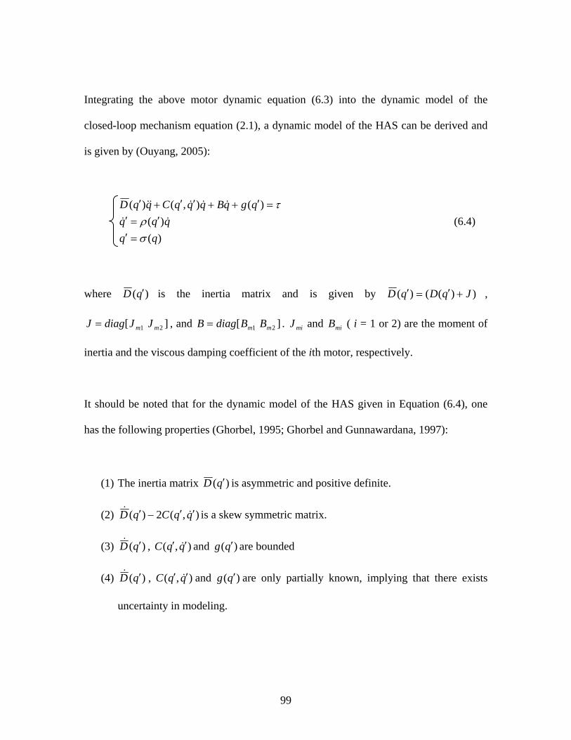
99
Integrating the above motor dynamic equation (6.3) into the dynamic model of the
closed-loop mechanism equation (2.1), a dynamic model of the HAS can be derived and
is given by (Ouyang, 2005):
)()(
)(),()(
qqqqq
qgqBqqqCqqD
σρ
τ
=′′=′
=′++′′+′
(6.4)
where )(qD ′ is the inertia matrix and is given by ))(()( JqDqD +′=′ ,
][ 21 mm JJdiagJ = , and ][ 21 mm BBdiagB = . miJ and miB ( i = 1 or 2) are the moment of
inertia and the viscous damping coefficient of the ith motor, respectively.
It should be noted that for the dynamic model of the HAS given in Equation (6.4), one
has the following properties (Ghorbel, 1995; Ghorbel and Gunnawardana, 1997):
(1) The inertia matrix )(qD ′ is asymmetric and positive definite.
(2) ),(2)( qqCqD ′′−′ is a skew symmetric matrix.
(3) )(qD ′ , ),( qqC ′′ and )(qg ′ are bounded
(4) )(qD ′ , ),( qqC ′′ and )(qg ′ are only partially known, implying that there exists
uncertainty in modeling.

100
Properties 1 and 2 can be proved as follows. Given that both )(qD ′ and J are symmetric
and positive definite (Ghorbel, 1995; Ghorbel and Gunnawardana, 1997), the matrix
))(()( JqDqD +′=′ is also symmetric and positive definite because J does not change in
time and is constant. The term ),(2)( qqCqD ′′−′ = ),(2)( qqCqD ′′−′ is skew (Ghorbel,
1995; Ghorbel and Gunnawardana, 1997; Ouyang 2005).
6.3 Sliding Mode Control (SMC) for nonlinear systems
For the control of nonlinear systems with parameter uncertainties, SMC is known as an
effective control approach. This approach originated in Russia in the late 1960’s and has
since been studied extensively for the control of nonlinear systems with modeling
uncertainties as well as the presence of time varying- parameter fluctuation and external
disturbances (Utkin, 1977; Slotine and Li, 1991; Edwards and Spurgeon, 1998; Ouyang
2005). The goal of this control approach is to constrain the states of the controlled system
to reach a given manifold in the state-space and thereafter slide towards an equilibrium
condition along this manifold (Ouyang, 2005). As applied to the control of the HAS, the
goal is to drive the joint position q to the desired position dq as close as possible, despite
the presence of the speed fluctuation 1q on the CV motor. As did previously, the tracking
errors are defined as the difference between the actual position and the desired one, i.e.,
d
d
qqeqqe
−=−=
(6.5)

101
where Tddd qqq ][ 21= and T
ddd qqq ][ 21= . As mentioned previously, link 1 is
connected to the CV motor, so tq dd ω=1 and ddq ω=1 . For SMC, the following sliding
surface is defined:
ees λ+= (6.6)
where ][ 21 λλλ diag= in which 1λ and 2λ are positive constants (i.e., control gains). In
addition, the following reference states are defined for the SMC:
eqsqqeqsqq
dr
dr
λλ
−=−=−=−=
(6.7)
As discussed in the preceding section, for the SMC control approach, it is assumed that
the dynamic model components, )(qD ′ , ),( qqC ′′ , and )(qg ′ are only partially known.
Let, let )(ˆ qD ′ , ),(ˆ qqC ′′ , and )(ˆ qg ′ denote the estimations of )(qD ′ , ),( qqC ′′ , and
)(qg ′ , respectively. Also let, )()(ˆ)( qDqDqD ′−′=′Δ , ),(),(ˆ),( qqCqqCqqC ′′−′′=′′Δ ,
and )()(ˆ)( qgqgqg ′−′=′Δ . Substituting Equations (6.5)-(6.7) into Equation (6.4), the
dynamic model of the hybrid mechanism in terms of the newly defined signal vector s,
can be written as follows:
⎥⎦
⎤⎢⎣
⎡+−Δ+−+−Δ+−
=+′′+′2222222
1111111),()(sBqBff
sBqBffBssqqCsqD
mm
mm
ττ
(6.8)

102
where
)(ˆ),(ˆ),(ˆ)(ˆ)(ˆ12121112121111 qgqqqcqqqcqqdqqdf rrrr ′+′′+′′+′+′= (6.9)
)(ˆ),(ˆ),(ˆ)(ˆ)(ˆ22221212221212 qgqqqcqqqcqqdqqdf rrrr ′+′′+′′+′+′= (6.10)
)(),()(][ 21 qgqqqCqqDfff rrT ′Δ+′′Δ+′Δ=ΔΔ=Δ (6.11)
For the CV motor it is assumed that the motor torque is constant. If the CV motor is
running at its operating speed, 1λ is equal to 0; and the motor torque is given by
dmB ωτ 11 = (6.12)
Further, the controlled torque for the servomotor is set as (Ouyang, 2005):
rrm assKfqB ττ +−−+= 222222 )sgn( (6.13)
where K is a design parameter, which is a positive constant; and rτ is the designed torque
of the servomotor to compensate for the speed fluctuations in the CV motor. Assume
bii ff Δ<Δ , where bifΔ is a positive constant, giving the boundary of ifΔ . The positive
constant K is chosen such that,
2bfK Δ≥ (6.14)
The designed torque rτ is based on the following switching rule:

103
=rτ 000,/)(
2
22111
=≠Δ+−
sifsifsffs b (6.15)
Furthermore, several remarks are given to the above SMC control law as applied to the
control of the HAS according to (Ouyang, 2005):
Remark 1. From Equation (6.13), it is observed that the torque applied to the
servomotor is not continuous. A smoothing method based on Slotine (1991) is used in
order to eliminate the chattering of the servomotor as follows:
0)/( 222222 >+−−+= φτφτ rrm assKsatfqB , (6.16)
where φ is called the boundary layer and must be greater than 0.
Remark 2. The designed torque for the servomotor in Equation (6.15) is discontinuous as
the sliding surface s is discontinuous. Therefore, Equation (6.15) is modified to eliminate
this chattering as follows:
=rτ 22
2111 )(s
sffs b
+
Δ+−
δ (6.17)
where δ is the boundary layer thickness and is greater than zero (i.e., )0>δ

104
6.4 Trajectory Planning for the CV and Servomotor
In this study, the CV motor is desired to rotate at a constant speed, while the servomotor
is planned in terms of the Hermite polynomial of the fifth degree. It is noted that for the
servomotor, such a planed trajectory results in bounded continuous position, velocity, and
acceleration profiles. The desired trajectories of both motors can be expressed as
ttq dd ω=)(1 (6.18)
))(10156()( 2023
3
4
4
5
5
202dd
ffff
dd qqtt
tt
ttqtq −+−+= (6.19)
where )(1 tq d and )(2 tqd are the desired trajectories of the two motors, dq20 and dfq2 are the
desired initial and final positions of the input link 2 driven by the servomotor,
ft represents the time required to reach the final position from the initial one. Two cases
with different operating speeds are set for experiments. As well for simplification, for
both operating speeds, 0)0(1 =q , 0)0(2 =q . In the experimental results presented in the
following section, the parameter values are set as, respectively:
Case 1:
πω 25.0=d (rad/s), dq20 =0, dfq2 =π , and ft =4s. (6.20)
Case 2:
πω 5.0=d (rad/s), dq20 =0, dfq2 =2π , and ft =4s. (6.21)

105
As can be seen from equations (6.20) and (6.21), the speed in Case 2 has doubled
compared to that of Case 1. For convenience, the first case is referred to as the low speed
case and the second one as the high speed case in the rest of this chapter.
6.5 Experimental Results of the HAS
The traditional PD control and the SMC control law are applied to the HAS mechanism.
The error between the desired motion and the actual motion is used to measure the
performance in this experimental study, as in the case of the RTC mechanism presented
in Chapter 5. The sampling periods for the traditional PD controller and the SMC are 4ms
and 10ms, respectively. The increase in the sampling time of the SMC is mainly due to
additional computational time required for this control law. From experimental
observation, the smallest sampling period attainable for the SMC control is 6ms.
However, since SMC heavily relies on velocity information, this sampling period was
increased to 10ms to obtain a smoother velocity profile.
The control parameters of the PD and SMC control laws are selected via trial and error
based on the criteria that was discussed in Chapter 5. In the case of the PD controller, pK
and pK are given as follows.
The low speed case:
Actuator 1 (servomotor): 00035.01 =pK , 000041.01 =dK
Actuator 2 (CV motor): Not real time controllable, i.e., no control gains

106
The high speed case:
Actuator 1 (servomotor): 00065.01 =pK , 000072.01 =dK
Actuator 2 (CV motor): Not real time controllable, i.e., no control gains
For the SMC control law, the controlled torque for the servomotor is chosen as in
Equation (6.16) with a = 0.00055 and 00045.02 =λ . Three case studies are performed at
the high speed operating condition and 3 are performed at the low speed operating
condition with the following control parameters:
Low Speed:
For Case 1: 5.0=δ , 5000.1=K , and 0000.1=φ
For Case 2: 7.0=δ , 5000.2=K , and 4000.1=φ
For Case 3: 9.0=δ , 0000.3=K , and 8000.1=φ
High Speed:
For Case 1: 5.1=λ , 3000.2=K , and 0000.2=φ
For Case 2: 4.2=λ , 5000.3=K , and 5000.2=φ
For Case 3: 5.2=λ , 4000.3=K , and 4000.2=φ
The physical parameters of the HAS prototype are previously presented in Figures 3.3
through 3.6 in Chapter 3, while the parameters of the two motors are listed in Table 6.1.

107
Table 6.1 The parameters of the two motors
Motor Type J (Kgm2) Bm (Nms)
CV motor 0.75 0.75 Servomotor 0.085 0.085
The position tracking errors or the difference between the measured angular position and
the desired ones are evaluated using the PD and SMC control laws. Figures 6.1 through
6.4 on the following pages illustrate the position tracking errors in the actuators as a
result of applying the PD and SMC controllers to the HAS, respectively. It should be
noted that the results presented for the comparison of the PD and SMC control laws
correspond to the parameters stated for Case 3 of the SMC at both the low and high speed
operating conditions, as these parameters resulted in the lowest position tracking errors in
the servomotor.

108
0
0.01
0.02
0.03
0.04
0.05
0.06
0.07
0 0.5 1 1.5 2 2.5 3 3.5 4
Time domain (sec)
Angl
e er
ror
(rad)
(a)
-0.08
-0.06
-0.04
-0.02
0
0.02
0.04
0.06
0 0.5 1 1.5 2 2.5 3 3.5 4
Time domain (sec)
Angl
e er
ror (
rad)
(b)
Figure 6.1: Measured position tracking errors in the motors for the low speed case using
PD controller: (a) angle error of Servomotor and (b) angle error of CV motor

109
-0.09
-0.07
-0.05
-0.03
-0.01
0.01
0.03
0.05
0.07
0 0.5 1 1.5 2 2.5 3 3.5 4
Time domain (sec)
Angl
e er
ror
(rad)
(a)
-0.1
-0.08
-0.06
-0.04
-0.02
0
0.02
0.04
0.06
0 0.5 1 1.5 2 2.5 3 3.5 4
Time domain (sec)
Angl
e er
ror (
rad)
(b)
Figure 6.2: Measured position tracking errors in the motors for the high speed case using
PD controller: (a) angle error of Servomotor and (b) angle error of CV motor

110
-0.07
-0.06-0.05
-0.04-0.03
-0.02-0.01
00.01
0.020.03
0 0.5 1 1.5 2 2.5 3 3.5 4
Time domain (sec)
Ang
le e
rror
(rad
)
(a)
-0.06-0.05-0.04-0.03-0.02-0.01
00.010.020.030.04
0 0.5 1 1.5 2 2.5 3 3.5 4
Time domain (sec)
Angl
e er
ror (
rad)
(b)
Figure 6.3: Measured position tracking errors in the motors for the low speed case using
SMC: (a) angle error of Servomotor and (b) angle error of CV motor

111
-0.06
-0.04
-0.02
0
0.02
0.04
0.06
0.08
0.1
0 0.5 1 1.5 2 2.5 3 3.5 4
Time domain (sec)
Angl
e er
ror (
rad)
(a)
-0.1
-0.08
-0.06
-0.04
-0.02
0
0.02
0.04
0.06
0 0.5 1 1.5 2 2.5 3 3.5 4
Time domain (sec)
Angl
e er
ror (
rad)
(b) Figure 6.4: Measured position tracking errors in the motors for the high speed case using
SMC: (a) angle error of Servomotor and (b) angle error of CV motor

112
From Figures 6.1 and 6.2, the maximum position tracking errors for the low speed
operating case using PD control are 0.059 rad and 0.072 rad for the servomotor and the
CV motor, respectively; and are 0.086 rad and 0.092 rad for the high speed case. The
results show satisfactory trajectory tracking at these operating speeds by using PD control,
although it was indicated by Ouyang (2005) that this controller is inadequate for such a
mechanism. This can be explained as follows. The maximum speed that the HAS
mechanism is operated at for this experimental study is 15 rpm. At this operating speed
however, the speed fluctuation of the CV motor is not considerably large enough to have
a significant impact on the servomotor. Nonetheless, it is interesting to note from Figure
6.1 that at lower speeds the position errors of the PD controller for the servomotor tend to
converge closer to zero compared to that of the high speed case. From these figures it can
be observed that the PD controller is not as effective at the higher speed case for the HAS.
This is due to the reason that at the higher operating speed scenario, the velocity
fluctuations of the CV motor is also larger, which the PD controller can not compensate
for.
As the speed of the mechanism increases, these velocity fluctuations become too large
and the PD controller becomes unstable. In such operating conditions, a controller such
as SMC that takes into account the velocity fluctuations of the CV motor is necessary for
the control of the HAS. From Figures 6.3 and 6.4, one can observe that the SMC control
law results in satisfactory performance and acceptable errors at both the low and high
speed operating conditions. Particularly, the maximum position tracking errors for the
low speed cases using SMC control are 0.057 rad and 0.052 rad for the servomotor and

113
the CV motor, respectively and are 0.084 rad and 0.089 rad for the high speed case. It
should be noted that at the higher speed operating condition, the position tracking errors
of the SMC control law converge to nearly zero, whilst those of the traditional PD
controller do not. This shows that the SMC controller is more effective than the PD
controller at the higher speed case.
6.6 Conclusion
In this chapter, the complete dynamic model of the HAS prototype including the dynamic
models of the servomotor and the CV motor are introduced. As well, SMC is reviewed
and outlined for the control of nonlinear time-varying systems with parameter
uncertainties. In the experimental study presented in this chapter, the traditional PD
control and the SMC are applied to the HAS. It was observed that at the speed examined
in this experimental study, PD control can result in satisfactory performance. It is also
observed that SMC proved to be more effective than the traditional PD control at higher
speeds. The reason for this is that the SMC control law can compensate for the velocity
fluctuation of the CV motor, whilst the traditional PD controller does not have this
capability. As the velocity fluctuation of the CV motor becomes larger at higher speeds,
the traditional PD controller becomes unstable and may not be adequate for the control of
the HAS.

114
Chapter 7 Conclusion and Recommendation 7.1 Overview of the thesis
RTC mechanisms and hybrid actuation systems are widely used in the industry. Recently,
several control approaches have been developed for the control of both RTC mechanisms
and hybrid actuation systems at the AEDL of the University of Saskatchewan. These
control approaches have proven to be promising through simulation studies, experimental
verification, however, remains to be addressed. This research is to carry out an
experimental study to examine and verify their effectiveness.
One of the major contributions of this research is the development of a generic
experiment environment where various control approaches can be examined and verified
experimentally. Particularly, two test beds, the RTC mechanism and the HAS, were
designed and developed for this purpose.
The other major contribution is the experimental examination and verification of several
control approaches. As applied to the RTC mechanism, the examined control approaches
include the traditional PD control, NPD control, iterative learning control techniques

115
(EPD, NPD-LC, and AES-PD), and the CTC approach. As applied to the HAS, the
traditional PD control and the SMC control technique are examined and compared.
7.2 Major Conclusions
(1) The RTC mechanism and the HAS, developed based on a 2-DOF closed-loop
mechanism is appropriate for the experimental examination and verification of
different control approaches.
(2) The experiments on the five PD-based control algorithms, i.e., PD control, NPD
control, EPD, NPD-LC, and AES-PD, show that the NPD controller has better
performance than the PD controller in terms of the reduction in position tracking
errors. It is also illustrated by the experiments that EPD, NPD-LC, and AES-PD are
all effective for use in situations where the task of the robot involves a repetition of
its trajectory. Moreover, AES-PD control technique was shown to be superior to
both the NPD-LC and the EPD in terms of the reduction in the position tracking
errors from iteration to iteration.
(3) Feedback and feedforward ILC are applied to the RTC mechanism. Experimental
results show that feedback ILC is more effective than the feedforward ILC and has
a faster convergence rate. In addition, the results of the comparative study of the
traditional PD and the CTC control technique at both low and high speeds show that
at lower speeds, both of these controllers provide similar results. However, with an

116
increase in speed, as the accuracy in the calculation of the dynamic model decreases,
the position tracking errors using the CTC control approach become larger than that
of the traditional PD control
(4) The experimental results of the HAS show that for the control of the hybrid
machine for the range of speed used in this experimental study, the traditional PD
control can result in satisfactory performance. However, with an increase in speed,
SMC proved to be more effective. SMC has the capability to cope with the velocity
fluctuation present in the system as a result of the presence of the CV motor. As the
speed increases and thereof a larger velocity fluctuation will be present, the
traditional PD controller can no longer compensate for this velocity fluctuation and
will become unstable. Therefore, at higher speeds a more sophisticated controller
such as SMC is required.
7.3 Future Work
The experiments and results presented in this thesis are based on some simplifications.
The results presented are acceptable for the purposes of demonstrating the validity and
effectiveness of the proposed control algorithms. For applications to the real situations,
however, some issues need to be further addressed, which include the initial position
error, the sampling period, and the estimation of velocity. In particular, for the problem
related to the initial position error, one solution would be to use an absolute position
encoder. As well, to reduce the sampling period for future possible improvement of the

117
control performance, one may use a hardware device such as dSPACE. In addition, for
the estimation of velocity, a low pass filter could be used for possible improvements.
In the experiments presented in this thesis, the motor speed to drive the mechanism was
set up to 15 rpm. With the current settings, the system was found to be inappropriate to
run at speeds higher than this speed due to the presence of the un-balanced forces. To
alleviate this problem, the individual linkages of the five-bar structure should be
redesigned so that the force balancing conditions can be achieved in the mechanism,
thereby possibly further improving the trajectory tracking performance.

118
REFERENCES Armstrong, B., and Wade, B. A., 2000, Nonlinear PID Control with Partial State
Knowledge: Damping without Derivatives, The International Journal of Robotics
Research, Vol.19, No. 8, pp. 715-731.
Arimoto, S., Kawamura, S., and Miyasaki, F., 1984, Bettering operation of robots by
learning, Journal of Robotic Systems, Vol.1, No.2, pp. 123-140.
Chen, Q.J., Chen, H. T., Wang, Y.J., and Woo, P.Y., 2001, Global stability analysis for
some trajectory tracking control schemes of robotic manipulators, Journal of Robotic
Systems, Vol. 18, No. 2, pp. 69-75.
Chen, Y. Q., and Moore, K. L., 2002, An optimal design of PD-type iterative learning
control with monotonic convergence, Proceedings of the 2002 IEEE International
symposium on Intelligent Control, pp. 55-60.
Codourey, A., 1998, dynamic modeling of parallel robots for computed-torque control
implementation, The International Journal of Robot Research, Vol. 17, No. 12, pp. 1325-
1136.

119
Constantinescu, D., and Croft, E.A., 2000, Smooth and time-optimal trajectory planning
for industrial manipulators along specified paths, Journal of Robotic Systems, Vol. 17,
No. 5, pp. 233-249.
Craig, J. J., 1986, Introduction to robotics: mechanics and control. Reading, Addison Wesley, MA.
Craig, J.J., 1988, Adaptive control of mechanical manipulators, Addison-Wesley.
Edwards, C. and Spurgeon, S. K., 1998, Sliding Mode Control Theory and Application,
Taylor & Francis Ltd, Padstow, UK.
Fitcher, E.F., 1986, A Stewart platform based Manipulator: General Theory and Practical
Construction, International Journal of Robotics Research, pp. 157-182.
Gautrier, M., Khalil, P., and Restrepo P., 1995, Identification of the dynamic parameters
of a closed-loop robot, in Proceedings of IEEE International Conference of Robot
Automat, pp. 3045-3050.
Ghorbel, F., 1995 Modeling and PD control of a closed-chain mechanical system,
Proceeding of 34th Conference on Decision & Control, New Orleans, LA, USA, pp. 540
542.
Ghorbel, F., 1997, A validation study of PD control of a closed chain mechanical system,
Proceeding of the 36th Conference on Decision & Control, San Diego, California, USA,

120
Dec., 1997, pp. 1998-2004.
Ghorbel, F., and Gunawardana, R., 1997, A validation study of PD control of a closed
chain mechanical system, Proceeding of the 36th Conference on Decision & Control, San
Diego, California, USA, Dec., 1997, pp. 1998-2004.
Ghorbel, F., and Srinivasan, B., 1998, On the uniform boundedness of the inertia matrix
of serial robot manipulators, Journal of Robotic Systems, Vol. 15, No. 1, pp. 17-28.
Ghorbel, F., Chetelat, O., and Longchamp, R., 1994, A reduced model for constrained
rigid bodies with application to parallel mechanical systems, Proceeding of the 4th IFAC
Symposium on Robot Control, Capri, Italy, pp. 45-50.
Greenough, J. D., Bradshaw, W. K., and Gilmartin, M. J., 1995, Design of hybrid
machines, Proceedings of the 9th World Congress on the Theory of Machines and
Mechanisms, pp. 2501-2505.
Guo, L. S., Zhang, W. J., Li, Y. F., and Li, Q., 1999, Design, Modelling and Control of a
Hybrid Machine, IEEE/ASME Trans on Mechatronics, Vol. 14, pp.324-332.
Hall, Jr., Allen S., 1981. Notes on Mechanism Analysis, Waveland Press, Prospect
Heights, Illinois.

121
IFToMM, 1991, Terminology for the theory of machines and mechanisms, Mechanism
and Machine Theory, Vol. 26, No. 5, pp. 435-439.
Kelly, R., 1997, PD control with desired gravity compensation of robotic manipulators: a
Review, The international Journal of Robotics Research, Vol. 16, No. 5, pp. 660-672.
Kerry, R., 1997, PD control with desired gravity compensation of robotic manipulators: a
review, The International Journal of Robotics Research, Vol.16, No. 5, pp. 660-672.
Klein, B. A. J., 1987, Kinematic optimization of mechanisms, a finite element approach,
Dissertation, Delft University of Technology, the Netherlands.
Kreyszig, E., 2002, Advanced Engineering Math, John Wiley and Sons.
Kuc, T. Y., Nam, K., and Lee, J. S., 1991, An iterative learning control of robot
manipulators, IEEE Trans. on Robotics and Automation, Vol. 7, No. 6, pp. 835-842.
Li, Q., and Wu, F. X., 2004, Control performance improvement of a parallel robot via the
design for control approach, Mechatronics, Vol.14, pp.947-964.
Li, Q., Tso, S. K., Guo, L. S., and Zhang, W. J., 2000, Improving motion tracking of
servomotor-driven closed-loop mechanisms using mass-redistribution, Mechanism and
Machine Theory, Vol. 35, No. 7, pp. 1033-1045.

122
Lin, C.S., Chang P.R., and Luh, J.Y.S., 1983, formulation and optimization of cubic
polynomial joint trajectories for industrial robots, IEEE trans. On Automatic Control, Vol.
AC-28, No. 12, pp. 1066-1074.
Liu, K., Lebret, G., and Lewis, F.L., 1993, Dynamic Analysis and Control of a SP
Manipulator, Journal of Robotic Systems, Vol. 10, No. 5, pp. 629-655.
Macfarlane, S., and Croft, E.A., 2001, Design of jerk bounded trajectories for on-line
industrial robot applications, Proceedings of the 2001 IEEE International Conference on
Robotics and Automation, Seoul, Korea, pp. 979-984.
Nasar, S. A., and Unnewehr, L. E., 1979, Electromechanics and Electric Machines, John
Wiley & Sons, New York.
Nguyen, P., and Cipra, R. J., 1999, Dynamic analysis of five-bar mechanism with
torsional springs using Lagrange’s equation and kinematic coefficients, 1999 ASME
Design Engineering Technical Conferences, DAC-8621, Las Vages, Nevada, USA.
Ouyang, P., 2002, “Force balancing design and trajectory tracking control of real-time
controllable mechanisms”, M.Sc. thesis, University of Saskatchewan.
Ouyang, P., 2005, “Hybrid Intelligent Machine Systems: Design, Modelling and control”,
Ph.D. thesis, University of Saskatchewan.

123
Ouyang, P. R., and Zhang, W. J., 2004, Comparison of PD-based Controllers for Robotic
Manipulators, Proceedings of the ASME Design Engineering Technical Conference, Vol.
2, pp. 23-31.
Ouyang, P. R., Zhang, W. J., and Gupta, M. M., 2004, Adaptive Nonlinear PD Learning
Control for Robot Manipulators, Proceedings of the ASME Design Engineering
Technical Conference, Vol. 2, pp. 357-365.
Ouyang, P. R., Zhang, W. J., and Gupta, M. M., 2004, A Robust PD-type Evolutionary
Learning Control for Nonlinear Time-varying systems, the 2004 IEEE International
Symposium on Intelligent Control, September 1 - 4, Taipei, Taiwan, pp. 90-95.
Paul, R. P., 1979, Manipulator Cartesian path control, IEEE Trans. System, Man, Cybern.,
Vol. SMC-9, Nov., pp. 702-711.
Qu, Z. H., 1994, Global stability of trajectory tracking of robot under PD control,
Dynamics and Control, Vol. 5, No. 1, pp. 59-71.
Qu, Z. H., 1995, Global stability of trajectory tracking of robot under PD control,
Dynamics and Control, Vol. 5, No. 1, pp. 59-71.
Raghavan, M., Waldron, K.J., and Roth, B., 1989, Kinematics of a Hybrid Series-Parallel
Manipulation System, AMSE J. of DMC., Vol.111, pp. 211-221.

124
Reboulet, C., and Berthomieu, T., 1991, Dynamic models of a Six Degree of Freedom
Parallel Manipulators, Proc. Of the Conf. ICAR 91, pp. 377-394.
Rugh, W. J., 1987, Design of nonlinear PID controllers, AIChE Journal, Vol. 33, No. 10,
pp. 1738-1742.
Seraji, H., 1998, Nonlinear and adaptive control of force and compliance in manipulators,
International Journal of Robotics Research, Vol. 17, No. 5, pp. 467-484.
Shahruz, S. M., and Schwartz, A. L., 1994, Design and optimal tuning of nonlinear PI
compensators, Journal of Optimization Theory and Applications, Vol. 83, No. 1, pp. 181-
198.
Slotine, J. E., and Li, W. P., 1991, Applied Nonlinear Control, Prentice Hall, Eaglewood
Cliffs, N. J.
Tayebi, A., 2003, Adaptive iterative learning control for robot manipulators, Proceedings
of the American Control Conference, pp.4518-4523.
Thomson, W. T., 1993, Theory of vibration with Applications, Prentice Hall, Englewood
Cliffs, New Jersey.
Tokuz, L.C. and Jones, J.R., 1991, Programmable modulation of motion using hybrid
machines, Proceedings of ImechE, C414/071, pp.85-91.

125
Tondu, B., and Bazaz S. A., The three-cubic method: an optimal online robot joint
trajectory generator under velocity, acceleration, and wandering constraints, The
International Journal of Robotics Research, Vol. 18, No. 9, pp. 893-901.
Utkin, V. I., 1977, Variable structure systems with sliding modes, IEEE Trans. On
Automatic Control, Vol. 22, No. 2, pp. 212-222.
Wang, Z. H., 2000, “Mechatronic design to real-time controllable mechanical systems:
force balancing and trajectory tracking”, M.Sc. thesis, University of Saskatchewan.
Xu, Y. M., Hollerbach, J. M., and Ma, D. H., 1995, A Nonlinear PD Controller for Force
and Contact transient control, IEEE Control Systems Magazine, Vol. 15, No. 1, pp. 15-21.
Youcef-Toumi, J., and Kuo, A. T. Y., 1993, High-speed trajectory control of a direct
drive manipulator, IEEE Trans. On Robotics and Automation, Vol. 9, pp. 102-108


