

CSE 555: Srihari 0
Non-Parametric Techniques
Generative and Discriminative Methods
Density Estimation
CSE 555: Srihari 1
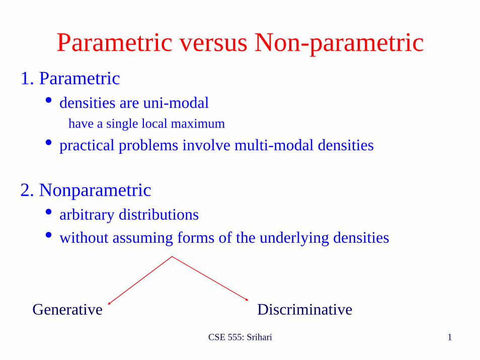
Parametric versus Non-parametric1. Parametric
• densities are uni-modal have a single local maximum
• practical problems involve multi-modal densities
2. Nonparametric• arbitrary distributions • without assuming forms of the underlying densities
Generative Discriminative

CSE 555: Srihari 2
Two types of nonparametric methods
1. Generative:Estimate class-conditional density p(x | ωj )1. Parzen Windows2. kn-nearest neighbor estimation
2. Discriminative:Bypass density estimation and go directly to compute a-posteriori probability P(ωj /x )1. nearest neighbor rule2. k-nearest neighbor rule

CSE 555: Srihari 3
Histograms are the heart of density estimationAn example of a histogram (feature called negative slope)

CSE 555: Srihari 4
More HistogramsEntropy No of black pixels
Exterior contours Interior contours

CSE 555: Srihari 5
Histogram for Horizontal slope Histogram for Positive slope

CSE 555: Srihari 6
Density Estimation
• Basic idea of estimating an unknown pdf:
• Probability P that a vector x will fall in region R is:
• P is a smoothed (or averaged) version of the density function p(x)• We can estimate the smoothed value of p by estimating the probability P
∫ℜ
= (1) 'dx)'x(pP
CSE 555: Srihari 7
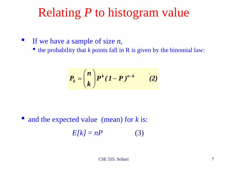
Relating P to histogram value
• If we have a sample of size n, • the probability that k points fall in R is given by the binomial law:
• and the expected value (mean) for k is:
E[k] = nP (3)
(2) )P1(P kn
P knkk
−−⎟⎟⎠
⎞⎜⎜⎝
⎛=

CSE 555: Srihari 8
Binomial Distribution
• This binomial distribution for kpeaks very sharply about the mean
• Therefore, the ratio k/n is a good estimate for the probability P and hence for the density function p
• Especially accurate when n is very large
(2) )P1(P kn
P knkk
−−⎟⎟⎠
⎞⎜⎜⎝
⎛=
nP k ≈

CSE 555: Srihari 9
Space average of p(x)
• If p(x) is continuous and the region R is so small that p does not vary significantly within it, we can write:
• where x is a point within R and • V the volume enclosed by R
(4) )(')'(∫ℜ
≅= VxpdxxpP

CSE 555: Srihari 10
Expression for p(x) from histogram
Combining equations (1), (3) and (4)
∫ℜ
= (1) 'dx)'x(pP
E[k] = nP (3)
(4) )(')'(∫ℜ
≅= VxpdxxpP
yields
Vn/k)x(p ≅

CSE 555: Srihari 11
(2) )P1(P kn
P knkk
−−⎟⎟⎠
⎞⎜⎜⎝
⎛=

CSE 555: Srihari 12
Practical and Theoretical Issues• The fraction is a space averaged value of p(x)
• p(x) is obtained only if V approaches zeroThis is the case where no samples are included in R and our estimate p(x) = 0
• Practically, V cannot be allowed to become small since the number of samples is always limited
• One will have to accept a certain amount of variance in the ratio k/n
Vn/k)x(p ≅
CSE 555: Srihari 13
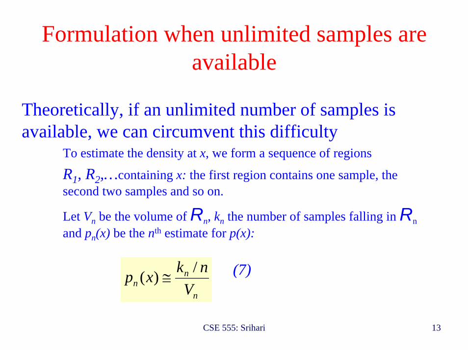
Formulation when unlimited samples are available
Theoretically, if an unlimited number of samples is available, we can circumvent this difficulty
To estimate the density at x, we form a sequence of regions
R1, R2,…containing x: the first region contains one sample, the second two samples and so on.
Let Vn be the volume of Rn, kn the number of samples falling in Rnand pn(x) be the nth estimate for p(x):
(7)n
nn V
nkxp /)( ≅

CSE 555: Srihari 14
Necessary conditions for convergence: pn(x) p(x)
0n/klim )3
klim )2
0Vlim )1
nn
nn
nn
=
∞=
=
∞→
∞→
∞→
n
nn V
nkxp /)( ≅
Two different ways of obtaining sequences of regions that satisfy these conditions:
(a) Shrink an initial region where Vn = 1/√n and show that
This is called “the Parzen-window estimation method”(b) Specify kn as some function of n, such as kn = √n; the volume Vn is
grown until it encloses kn neighbors of x. This is called “the kn-nearest neighbor estimation method”
)x(p)x(pnn ∞→→
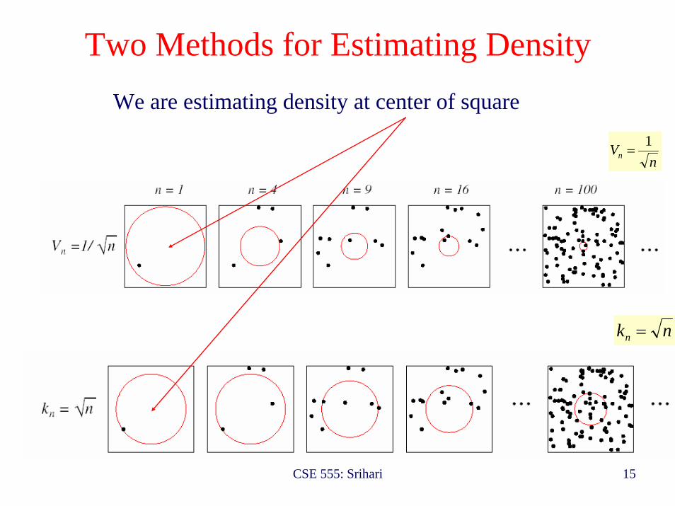
CSE 555: Srihari 15
Two Methods for Estimating DensityWe are estimating density at center of square
Method 1: start with large volume centered at point and shrink it according to nVn
1=
Method 2: start with large volume centered at point and shrink it according to nkn =

CSE 555: Srihari 16
Parzen Window Method• Unit hypercube function
⎪⎩
⎪⎨⎧ =≤
=otherwise 0
d , 1,...j 21u 1
(u)
:function windowfollowing thebe (u)
jϕ
ϕLet 1u
u1
u2
u3
CSE 555: Srihari 17
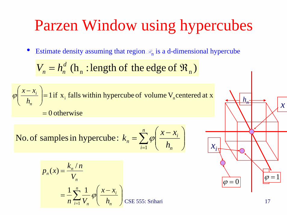
Parzen Window using hypercubes• Estimate density assuming that region Rn is a d-dimensional hypercube
) of edge theoflength :(h nn ℜ= dnn hV
otherwise 0
at x centeredV volumeof hypercube within falls xif 1 ni
=
=⎟⎟⎠
⎞⎜⎜⎝
⎛ −
n
i
hxxϕ hn x
1=ϕ0=ϕ
∑=
⎟⎟⎠
⎞⎜⎜⎝
⎛ −=
n
i n
in h
xxk1
:hypercubein samples of No. ϕ
⎟⎟⎠
⎞⎜⎜⎝
⎛ −=
=
∑= n
in
i n
n
nn
hxx
Vn
Vnkxp
ϕ1
11
/)(
xi
CSE 555: Srihari 18
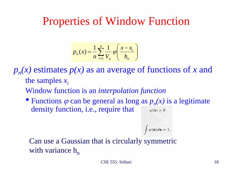
Properties of Window Function
pn(x) estimates p(x) as an average of functions of x and the samples xiWindow function is an interpolation function• Functions ϕ can be general as long as pn(x) is a legitimate
density function, i.e., require that
⎟⎟⎠
⎞⎜⎜⎝
⎛ −= ∑
= n
in
i nn h
xxVn
xp ϕ1
11)(
Can use a Gaussian that is circularly symmetric with variance hn

CSE 555: Srihari 19
Effect of window-width on estimate pn(x))(1)( then 1)(
1i
n
inn
nnn xx
nxp
hx
VxLet −=⎟⎟
⎠
⎞⎜⎜⎝
⎛= ∑
=
δϕδ
Gaussianwindowswithdecreasing widths
Parzen windowestimates usingfive samples
For any hn, distribution isis normalized, i.e.,
Out-of-focus estimate Erratic estimate
CSE 555: Srihari 20
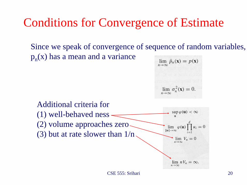
Conditions for Convergence of Estimate
Since we speak of convergence of sequence of random variables,pn(x) has a mean and a variance
Additional criteria for(1) well-behaved ness (2) volume approaches zero (3) but at rate slower than 1/n
CSE 555: Srihari 21
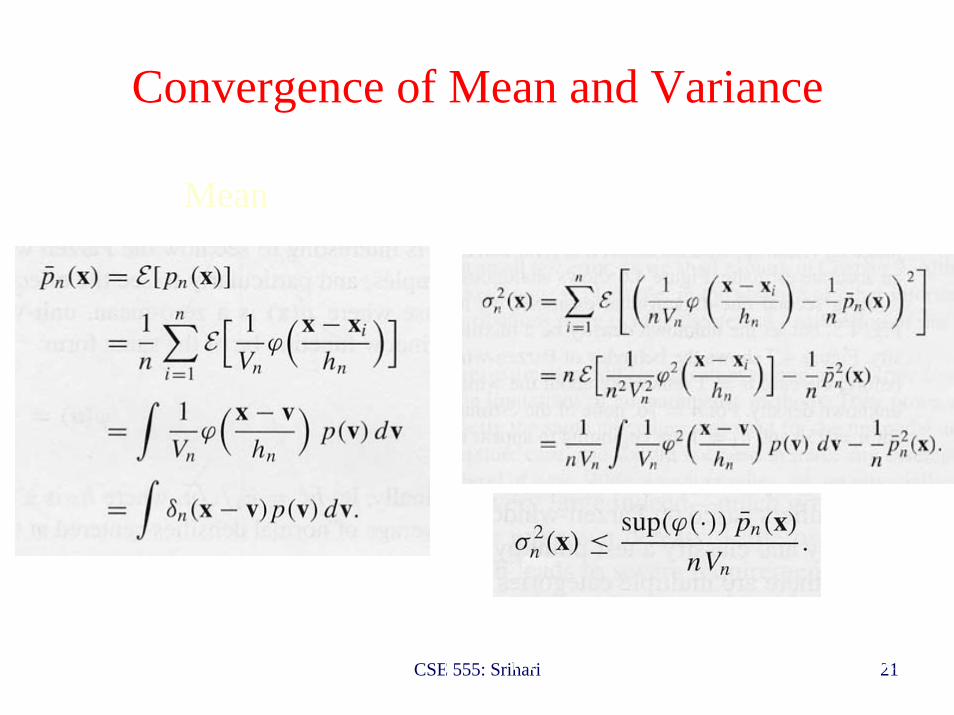
Convergence of Mean and Variance
MeanVariance
Conclusion:expected value of estimate isconvolution of unknowndensity and window function
Conclusion: let Vn=V1/sqrt(n) or V1/ln n etc

CSE 555: Srihari 22
Example of Parzen Window on simple cases
Case where p(x) N(0,1)
is an average of normal densities
centeredat the samples xi.
⎟⎟⎠
⎞⎜⎜⎝
⎛ −= ∑
=
= n
ini
1i nn h
xx h1
n1)x(p ϕ
nhheu nu / and
21)( 1
2/2
== −
πϕ
Contributions of samples clearly observable)1,x(N)xx(e21 )xx()x(p 1
21
2/111 →−=−= −
πϕ
Univariate normal Bivariate normal
CSE 555: Srihari 23
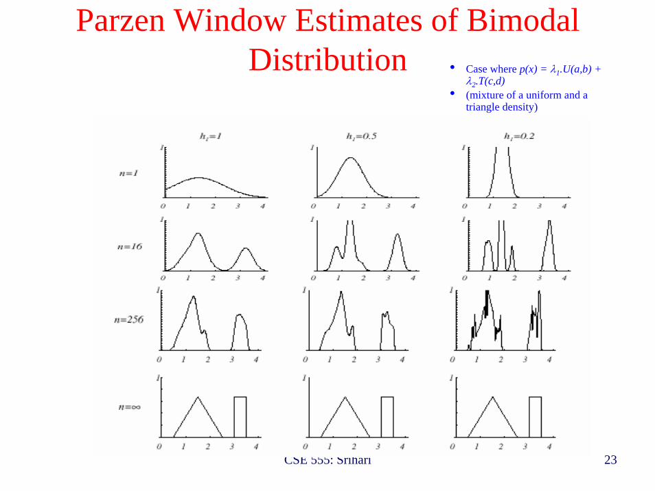
Parzen Window Estimates of Bimodal Distribution
Window widths
No.OfSamples
• Case where p(x) = λ1.U(a,b) + λ2.T(c,d)
• (mixture of a uniform and a triangle density)
As no of samples become large estimates are same with each window width
CSE 555: Srihari 24
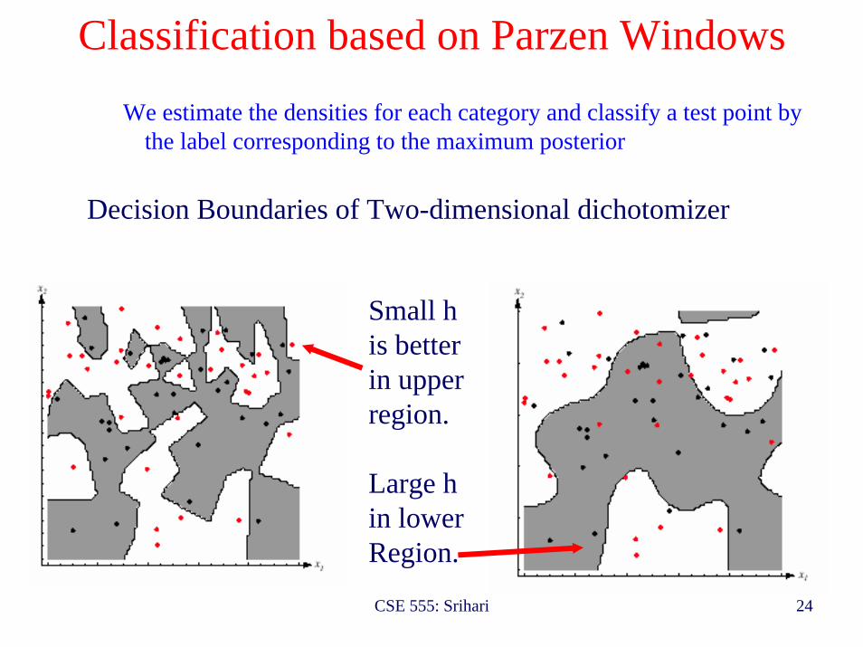
Classification based on Parzen WindowsWe estimate the densities for each category and classify a test point by
the label corresponding to the maximum posterior
Decision Boundaries of Two-dimensional dichotomizerUsing small h Using large h
Small his betterin upperregion.
Large hin lowerRegion.

CSE 555: Srihari 25
Parzen Window Conclusion
• No assumptions made ahead of time regarding distributions
• Same procedure was used for unimodal and bimodal cases• With enough samples assured of convergence
• May need large no of samples however• Also, no data reduction provided which leads to severe
computation and storage requirements• Demand for no of samples grows exponentially with
dimensionality

CSE 555: Srihari 26
Probabilistic Neural Networks
Parzen Window Method can be implemented as an artificial neural network Connections
correspondto class labels ofpatterns
FeatureValuesOf Patterns
WeightVector w

CSE 555: Srihari 27
Probabilistic Neural Networks
Parzen Window Method can be implemented as an artificial neural network
an2
FeatureValuesOf Patterns
WeightVector w
a1c
CSE 555: Srihari 28
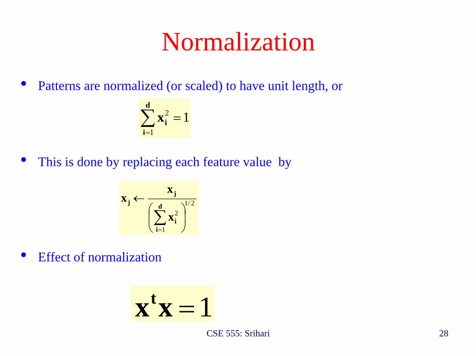
Normalization• Patterns are normalized (or scaled) to have unit length, or
• This is done by replacing each feature value by
• Effect of normalization
11
2 =∑=
d
iix
2/1
1
2 ⎟⎠
⎞⎜⎝
⎛←
∑=
d
ii
jj
x
xx
1=xxt
CSE 555: Srihari 29
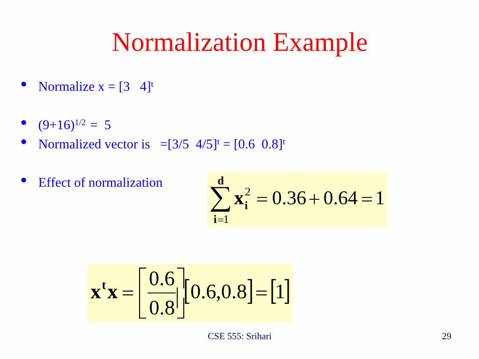
Normalization Example• Normalize x = [3 4]t
• (9+16)1/2 = 5• Normalized vector is =[3/5 4/5]t = [0.6 0.8]t
• Effect of normalization164.036.0
1
2 =+=∑=
d
iix
[ ] [ ]18.0,6.08.06.0
=⎥⎦⎤
⎢⎣⎡=xxt

CSE 555: Srihari 30
Activation Function
Contribution of a sample at xHere we let weights correspondto feature values of sample
( ) ( ) 22/ σαϕ kt
k wxwx
n
k eh
wx −−−⎟⎟⎠
⎞⎜⎜⎝
⎛ −
( ) ( )
2
2
2
/)1(
2/)2(
2/
σ
σ
σ
−
−+−
−−−
=
=k
kt
ktk
t
kt
k
net
wxwwxx
wxwx
e
e
exwnet t
kk =
Simplified form due tonormalization
1== ktk
t wwxx

CSE 555: Srihari 31
PNN Training Algorithm
Only connectionsCorresponding to class labels are set to 1
NormalizeFeature values
Set weights equalto feature values
Over all samples j
Over all features k
The aji correspond to making connections betweenlabeled samples and the corresponding classes
CSE 555: Srihari 32
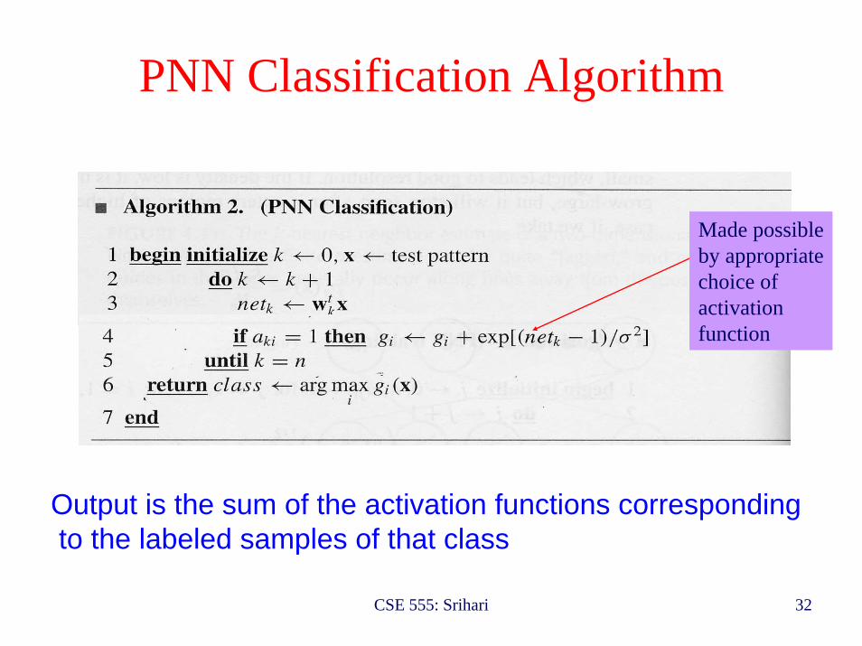
PNN Classification Algorithm
Made possibleby appropriatechoice ofactivationfunction
Output is the sum of the activation functions correspondingto the labeled samples of that class

CSE 555: Srihari 33
..
Parzen/PNN Classifier Stage 1
• Inputs: d normalized features• Weights correspond to feature values of n labeled samples
wij = xij, i=1,.., n; j=1,..,d • Input units are fully connected to n sample units.
.
.
.
Input unit Labeledsampleunits
.
. ..
Wnd
W2d
W11
nkxwnet tkk ,..1; ==
p1
p2
pn
x1
x2
xd
.
.
.

CSE 555: Srihari 34
.
.p1
p2
pn
.
.
.
sample patterns
PNN Stage 2: outputs are sparsely connected
pn
pk...
.
.ω1
ω2
ωc...
Category units
.
.
.
Activation functions (nonlinear functions)
2/)1( σ−knete
CSE 555: Srihari 35
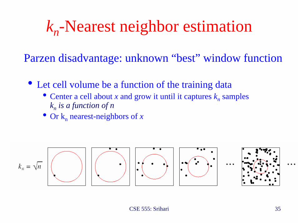
kn-Nearest neighbor estimation
Parzen disadvantage: unknown “best” window function
• Let cell volume be a function of the training data• Center a cell about x and grow it until it captures kn samples
kn is a function of n • Or kn nearest-neighbors of x
n = 1 n = 4 n = 9 n = 16 n = 100
CSE 555: Srihari 36
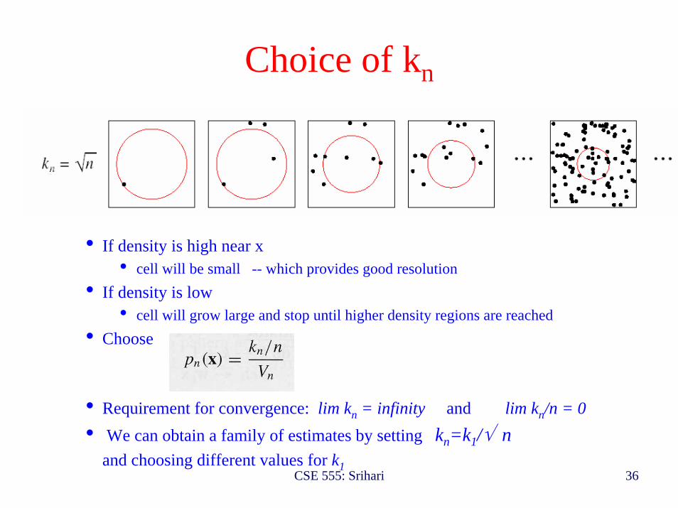
Choice of kn
• If density is high near x• cell will be small -- which provides good resolution
• If density is low• cell will grow large and stop until higher density regions are reached
• Choose
• Requirement for convergence: lim kn = infinity and lim kn/n = 0• We can obtain a family of estimates by setting kn=k1/√ n
and choosing different values for k1
CSE 555: Srihari 37
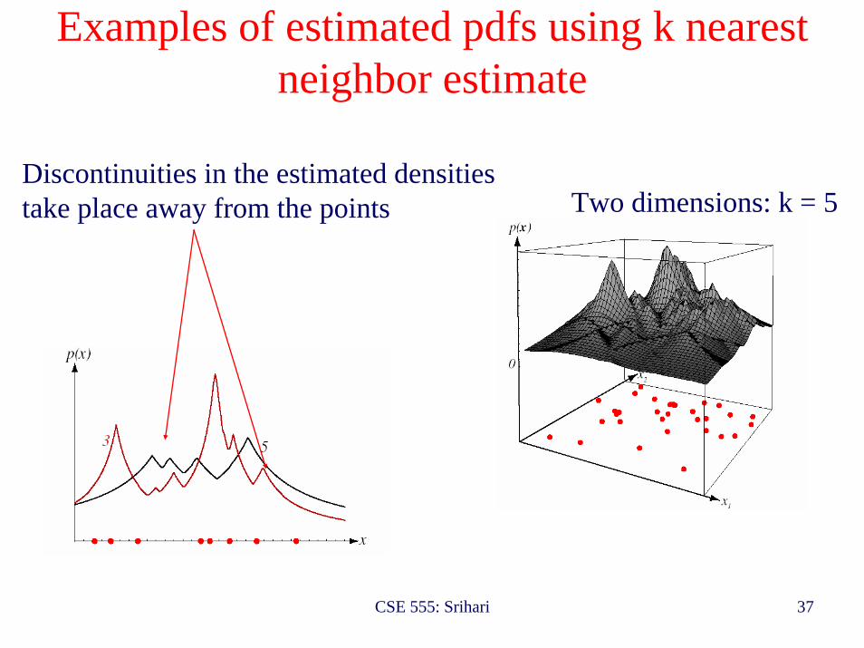
Examples of estimated pdfs using k nearest neighbor estimate
Two dimensions: k = 5
One dimension: k= 3 and 5
Discontinuities in the estimated densities take place away from the points

CSE 555: Srihari 38
Comparison of Parzen and k nnestimates in one-dimension
For k-nearest neighbor estimation using kn = √n = 1the estimate becomes
pn(x) = kn / n.Vn= 1 / V1=1 / 2|x-x1|
Clearly a poor estimate
Whereas Parzen yields:
k-nnestimate
Parzenestimate

CSE 555: Srihari 39
Examples of kn-Nearest-Neighbor EstimationBi-modalGaussian
Spiky estimateswhen there arefew samples

CSE 555: Srihari 40
Estimation of a-posteriori probabilities
kk
xp
xpxP
Vnkxp
ic
jjn
inin
iin
==
=
∑=1
),(
),()/(
/),(
ω
ωω
ωProduct ofclass-conditionaland a posterioriis represented amongsamples
• ki/k is the fraction of the samples within the cell that are labeled ωi
• For minimum error rate, the most frequently represented categorywithin the cell is selected
• If k is large and the cell sufficiently small, the performance will approach the best possible
• Size of the cell can be chosen using either Parzen or kn nearest neighbor


