

Monday28. December 2005
MGA Molecular Genome Analysis -Bioinformatics and Quantitative Modeling
Microarrays: Quality Control, Normalization and Experimental Design
Achim Tresch
Deutsches Krebsforschungszentrum
Molecular Genome Analysis
Bioinformatics/Biostatistics
Heidelberg, INF 580

Monday28. December 2005
MGA Molecular Genome Analysis -Bioinformatics and Quantitative Modeling
Overview• Introduction to microarray technologies• Image Processing:
Spot Identification, Spot/Background quantification, Quality Measures
• Normalization: Scaling, Quantile, Lowess, vsn
• Experimental Design: Comparison of typical Designs
• Affy Issues

Achim Tresch Molecular Genome Analysis
****
*
GeneChip Affymetrix
cDNA microarray
Nylon membrane
Agilent: Long oligo Ink Jet
Illumina Bead Array
CGH
SAGE
Different Technologies for Measuring Gene
Expression
1975: Southern Blotting Technology (Edward Southern)
1991: First high-density Nylon filter Arrays (Lennon, Lehrach)
1995: cDNA-Microarrays (Schena et al.)
1996: Affymetrix Genechip Technology (Lockhart et al.)

Achim Tresch Molecular Genome Analysis
cDNA and Affymetrix (short, 25 bp) Oligo Technologies.Long Oligos (60-75 bp) are used similar to cDNA.

Achim Tresch Molecular Genome Analysis
Biological verification and interpretation
Microarray experiment
Experimental design
Image analysis
Normalization
Biological question (hypothesis-driven or explorative)
TestingEstimation DiscriminationAnalysis
Clustering
Experimental
Cycle
Quality Measurement
Failed
Pass
Pre-processing
To call in the statistician after the experiment is done may be no more than asking him to perform a post-mortem examination: he may be able to say what the experiment died of.
Ronald Fisher

Achim Tresch Molecular Genome Analysis
Preprocessing result: Gene expression Matrix
Gene
mRNA Samples
Gene expression Level for Gen i in mRNA sample j
Log(red intensity / green intensity)
Function (PM, MM) of MAS, dchip or RMA
sample1 sample2 sample3 sample4 sample5 …
1 0.46 0.30 0.80 1.51 0.90 ...2 -0.10 0.49 0.24 0.06 0.46 ...3 0.15 0.74 0.04 0.10 0.20 ...4 -0.45 -1.03 -0.79 -0.56 -0.32 ...5 -0.06 1.06 1.35 1.09 -1.09 ...
Gene expression-Data for G Genes and n Hybridiyations. Genes times Arrays Data-Matrix:

Achim Tresch Molecular Genome Analysis
Data Data (log scale)
Preprocessing result visualization: Scatterplot(s)

Monday28. December 2005
MGA Molecular Genome Analysis -Bioinformatics and Quantitative Modeling
Image Analysis
• Spot identification• Spot quantification• Probe level quality control• Gene level quality control• Array level quality control• Example

Achim Tresch Molecular Genome Analysis
Spot Identification
• The grid structure is provided by the manufacturer or generated individually for custom-made microarrays (e.g. GAL-files)
• The grid is overlaid by hand or automatically onto the image (beware of column/row displacement errors!)
GAL-file contains Clone-IDs and defines their position on the grid
Columns
Row
s
Blocks

Achim Tresch Molecular Genome Analysis
Spot identification
• Individual spots are recognized, size and shape might be adjusted per spot (automatically fine adjustments by hand).
• Additional manual flagging of bad (X) or non-present (NA) spots
poor spot quality good spot quality
Different Spot identification methods: Fixed circles, circles with variable size, arbitrary spot shape (morphological opening)
NA
X

Achim Tresch Molecular Genome Analysis
Histogram of pixel intensities of a single spot
Spot quantification
• The signal of the spots is quantified.
„Donuts“
Mean / Median / Mode / 75% quantile
Achim Tresch Molecular Genome Analysis
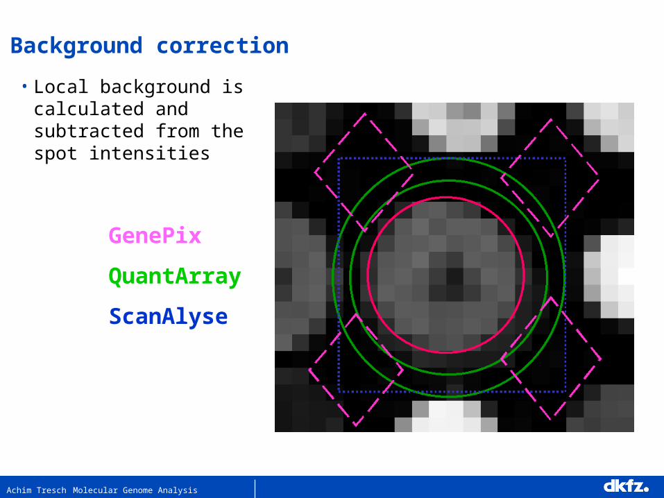
Background correction
• Local background is calculated and subtracted from the spot intensities
GenePix
QuantArray
ScanAlyse
Achim Tresch Molecular Genome Analysis
Quality control: Noise and reliable signal
• Is the signal dominated by noise? Acceptable amount of noise?
• Quantify noise (biol./technical variability)
• Quantify quality of a signal
• Guidelines for reasonable thresholds on the quality of a signal
• Defining strategies for exclusion of probes
• Probe level: quality of the expression measurement of one spot
on one particular array
• Array level: quality of the expression measurement on one
particular glass slide
• Gene level: quality of the expression measurement of one probe
across all arrays

Achim Tresch Molecular Genome Analysis
Probe-level (Individual spots) quality control
• Sources of Variability:• faulty printing, uneven distribution, contamination with debris, poorly
measured spots• Visual inspection:
• hairs, dust, scratches, air bubbles, dark regions, regions with haze• Spot quality measures:
• Brightness: foreground/background ratio• Uniformity: variation in pixel intensities and ratios of intensities within a
spot• Morphology: area, perimeter, circularity.• Spot Size: number of foreground pixels
• Action:• set measurements to NA (missing values)• use weights for measurements to indicate reliability in later analysis.

Achim Tresch Molecular Genome Analysis
Gene g
Gene-level quality control
• Poor hybridization in the reference channel may introduce bias on the fold-change
Arrays 1 ... n

Achim Tresch Molecular Genome Analysis
Gene-level quality control:Poor Hybridization and Printing
• Sources of Variability:
• Some probes will not hybridize well to the target RNA
• Printing problems such that all spots of a given print tip will have poor
quality.
• A well may be of bad quality (contamination, wrong RNA)
• Quality measure: Genes with a consistently low signal in the reference
channel are suspicious: Median of the background adjusted signal < 200*
*or other appropriate choice
• Action: Exclude gene from further analysis

Achim Tresch Molecular Genome Analysis
Gene-level quality control:Probe quality control based on duplicated spots
• Printing different probes that target the same gene or printing multiple copies of the same probe.
• Mean squared difference of log2 ratios between spot r and s:
MSDLR = (xjr – xjs)²/J sum over arrays j = 1, …, J
recommended threshold to assess disagreement: MSDLR > 1
• Disagreement between copies: printing problems, contamination, mislabeling. Not easy if there are only 2 or 3 slides.
Jenssen et al (2002) Nucleic Acid Res, 30: 3235-3244. Theoretical background

Achim Tresch Molecular Genome Analysis
Array-level quality control
• Problems:• array fabrication defect• problem with RNA extraction• failed labeling reaction• poor hybridization conditions• faulty scanner (wrong calibration)
• Quality measures:• Percentage of spots with no signal (~30% exlcuded spots) • Range of intensities• (Av. Foreground)/(Av. Background) > 3 in both channels• Distribution of spot signal area

Achim Tresch Molecular Genome Analysis
Swirl Data
• Experiment to study early development in zebrafish.
• Swirl mutant vs. wild-type zebrafish affecting development of dorsal-ventral
structures
• Two sets of dye-swap experiments.
• Microarray containing 8448 cDNA probes
• 768 control spots (negative, positive, normalization)
• printed using 4x4 print-tips, each grid contains a 22x24 Spot matrix
RR R Console
> library(marray)
> data(swirl)
> ll()
member class mode dimension1 swirl marrayRaw list c(8448,4)

Achim Tresch Molecular Genome Analysis
24 x 22spots per print-tip
MT – RWT - G
MT – GWT - R
Hybr. I
Hybr. II
Swirl Data

Achim Tresch Molecular Genome Analysis
4 x 4 sectors
Sector:24 rows22 columns
8448 spots
Mean signal intensity
Visual inspection
RR R Console
> image(swirl[,1])
81: image of M1 2 3 4
4
3
2
1
-5
-3.9
-2.8
-1.7
-0.56
0.56
1.7
2.8
3.9
5

Achim Tresch Molecular Genome Analysis
81: image of Rb1 2 3 4
4
3
2
1
58
300
540
780
1000
1300
1500
1700
2000
2200
81: image of Rf1 2 3 4
4
3
2
1
160
6800
13000
20000
27000
33000
40000
47000
53000
60000
81: image of Gb1 2 3 4
4
3
2
1
76
100
130
150
180
200
230
250
280
300
81: image of Gf1 2 3 4
4
3
2
1
160
6300
13000
19000
25000
31000
37000
43000
50000
56000
Visual inspection – Foreground and Background intensities
RR R Console
> Gcol <- maPalette( low = "white", high = "green", k = 50)
> Rcol <- maPalette( low = "white", high = "red", k = 50)
> image(swirl[,1] xvar="maRb", col=Rcol)
> image(swirl[,1] xvar="maRf", col=Rcol)
> image(swirl[,1] xvar="maGb", col=Gcol)
> image(swirl[,1] xvar="maRf", col=Gcol)
Achim Tresch Molecular Genome Analysis
200 500 1000 5000 20000 50000
10
02
00
50
01
00
02
00
0
Foreground (red)
Ba
ckg
rou
nd
(R
ed
)
swirl.1.spot
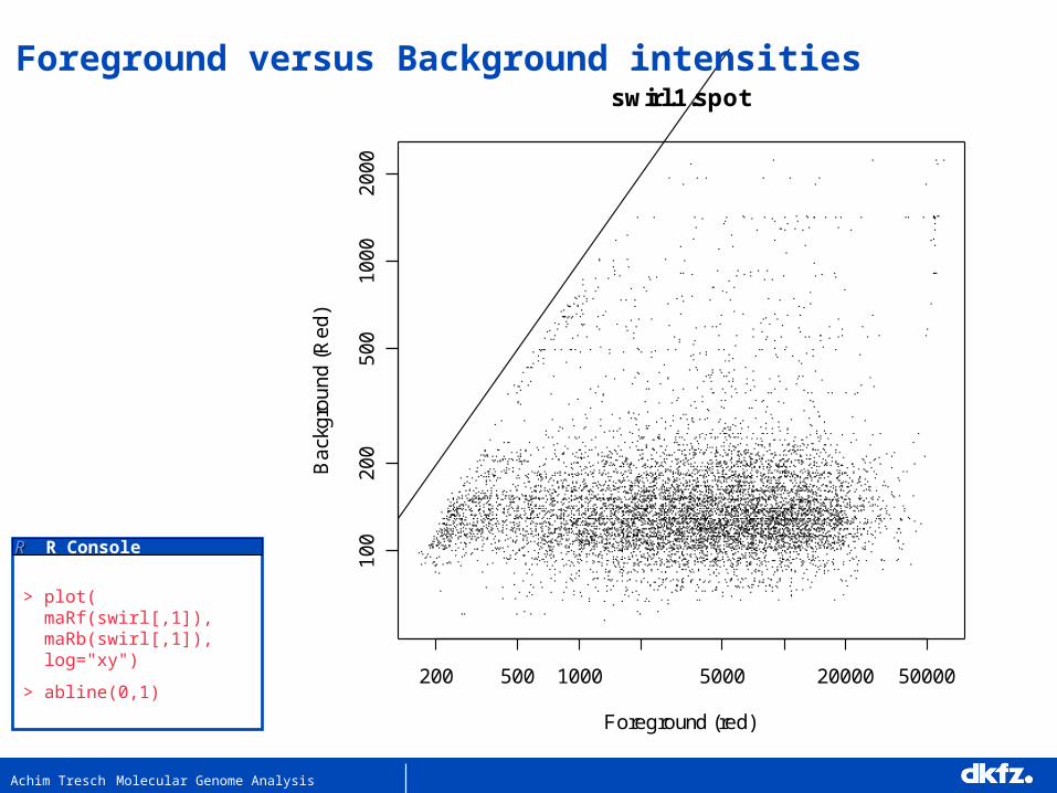
Foreground versus Background intensities
RR R Console
> plot( maRf(swirl[,1]), maRb(swirl[,1]), log="xy")
> abline(0,1)

Monday28. December 2005
MGA Molecular Genome Analysis -Bioinformatics and Quantitative Modeling
Normalization Methods
• Sources of Variation• Scaling Methods• Quantile Normalization• Lo(w)ess Normalization• Variance Stabilization

Achim Tresch Molecular Genome Analysis
Sources of Variation: Bias and Variance
biased unbiased
low noise
high noisex

Achim Tresch Molecular Genome Analysis
Sources of Variation for Microarray-Data
Normalization Error model
Systematic Stochastic• similar effect on many
measurements• corrections can be
estimated from data
• Effects on single spots• random effects that cannot
be estimated, „noise“
Remove bias Quantify variance

Achim Tresch Molecular Genome Analysis
tissue contamination
spot sizehybridization efficiency and specificity
amplification efficiency
stray-/background signal
Sources of Variation for Microarray-Data
Systematic Stochastic
amount of RNA in biopsy
efficiency of: RNA extraction, reverse transcription, labeling, photodetection
DNA support binding
spotting efficiency
reverse transcription efficiency
DNA quality
stray-/background signal RNA degradation
DNA quality
efficiency of: RNA extraction, reverse transcription, labeling, photodetection
stray-/background signal RNA degradation
spotting efficiency
reverse transcription efficiencyDNA support binding
amount of RNA in biopsy
tissue contamination
amplification efficiency
hybridization efficiency and specificityspot size

Achim Tresch Molecular Genome Analysis
Array 2Cy3 Cy5Array 1
Cy3 Cy5
median
Q3=75% Quantile
Q1=25% Quantile
Minimum
Maximum
Displaying Variability of Microarray-Data

Achim Tresch Molecular Genome Analysis
• Identify and remove sources of systematic variation, other than differential expression, in the measured fluorescence intensities.
Aims of normalization:
Enable the estimation of
• True fold changes
• Significance of differential expression
These aims can be adverse! Depending on the further analysis steps, different normalization strategies may be appropriate!

Achim Tresch Molecular Genome Analysis
Normalization via rescaling
81 82 93 94
-20
24
Swirl arrays: pre--normalization
M
boxplots
“Location and scale of different MA measurements should be (approximately) the same.“
• Location and scale are basic statistical concepts for data description:
Location normalization: corrects for spatial or dye bias
Scale normalization: homogenizes the variability across arrays
Normalized log-intensity ratios are given by
Mnorm = (M-location) / scale

Achim Tresch Molecular Genome Analysis
• Location: Robust estimation of a “rescaling” Factor, e.g. based on the median of gene expression values on the chip. The underlying assumption is that the majority of genes and hence the center of the expression values should not change between different measurements. The median is used as a robust measure for the center of a dataset.
• Scale: Use some measure for the variability of the data, e.g.
MAD = MedianAbsoluteDifference = median{ |x1-median|, …, |xn-median| }
( the MAD is a more robust measure of scale than the variance)
→ Median centering: Subtract the median of all expression values of one chip and divide by the MAD.
• Housekeeping genes
• Spiked in control genes
Normalization via rescaling

Achim Tresch Molecular Genome Analysis
(1,1
)
(1,2
)
(1,3
)
(1,4
)
(2,1
)
(2,2
)
(2,3
)
(2,4
)
(3,1
)
(3,2
)
(3,3
)
(3,4
)
(4,1
)
(4,2
)
(4,3
)
(4,4
)
-2-1
01
2
Swirl array 93: pre-norm
PrintTip
M
81 82 93 94
-20
24
Swirl arrays: pre--normalization
M
RR R Console
> boxplot(swirl[, 3], xvar = "maPrintTip", yvar = "maM")
> boxplot(swirl, yvar = "maM")
marray – Swirl Data: Raw data

Achim Tresch Molecular Genome Analysis
(1,1
)
(1,2
)
(1,3
)
(1,4
)
(2,1
)
(2,2
)
(2,3
)
(2,4
)
(3,1
)
(3,2
)
(3,3
)
(3,4
)
(4,1
)
(4,2
)
(4,3
)
(4,4
)
-10
12
3
Swirl array 93: post-norm
PrintTip
Mmarray – Swirl Data: Post Normalization
RR R Console
> swirl.norm <- maNorm(swirl, norm = "p")
> boxplot(swirl.norm[, 3], xvar = "maPrintTip", yvar = "maM")
> boxplot(swirl.norm, yvar = "maM")

Achim Tresch Molecular Genome Analysis
Swirl Data – M values, raw vs preprocessed and rescaled
81: image of M1 2 3 4
4
3
2
1
-5
-3.9
-2.8
-1.7
-0.56
0.56
1.7
2.8
3.9
581: image of M
1 2 3 4
4
3
2
1
-6
-4.7
-3.3
-2
-0.67
0.67
2
3.3
4.7
6
Normalization procedure was not able to remove scratchRR R Console
> image(swirl[,1])
> image(swirl.norm[,1])

Achim Tresch Molecular Genome Analysis
Problems with Median-Centering
Log Green
Log
Red
Scatterplot of log-Signals after Median-centering
A = (Log Green + Log Red) / 2
M =
Log
Red
- Lo
g G
reen
M-A Plot of the same data
Median-Centering is a global Method. It does not adjust for local effects, intensity dependent effects, print-tip effects, etc.
(M for Minus, A for Average)

Achim Tresch Molecular Genome Analysis
Quantile Normalization
QQ-plot
Distribution 1
Distribution 2

Achim Tresch Molecular Genome Analysis
Quantile Normalization
The basic idea of Quantile-Normalization is very simple:
„The Histograms of all Slides are made identical“
Tightens the idea of Median-Centering. Not only the 50%-Quantile is adjusted, but all Quantiles.
Boxplot and QQ-plot after Quantile normalization

Achim Tresch Molecular Genome Analysis
The Algorithm:
• For each array, sort the genes by expression
• Let Mn be the mean value of the nth genes of each array. Replace the values for the nth gene by Mn in each array.
• Do this for all positions n.
Disadvantage: For genes at the extreme ends of the distribution, the expression values of the nth genes have a high variance, so the mean may vary strongly. In general, quantile normalization tends to underestimate expression values at the high end and vice versa at the low end.
Quantile Normalization
Before using quantile normalization, measurement data for each chip should be on the same scale!

Achim Tresch Molecular Genome Analysis
Lo(w)ess Normalization
Assumption: There is an intensity-dependent bias of the fold change,
and hencewhere δj is the “true“ log fold change for gene j. The true fold change distribution is approximately a zero-symmetric normal distribution.
Task: Find f, replace yj by yj - f(xj).
)()(ˆ xfxf x
A = (Log Green + Log Red) / 2
M =
Log
Red
- Lo
g G
reen
f
)(AfM
jjj xfy )(
The idea of local regression is that f can be estimated locally at a point x by a simple (and easy-to-fit) function fx. For each point x, we then estimate f by

Achim Tresch Molecular Genome Analysis
In practice, fx is a polynomial of low order (≤ 2). Which points (and with which weights) are used to estimate fx is determined by a kernel weight function K.
Lo(w)ess Normalization
Taken from Tibshirani et al., „Elements of Statistical Learning“
N
jxjjx
xx
yxxK
tf
x 1
2])[,(argminˆ
, ˆ)(
N
jjxxjjxx
xxx
xyxxK
ttf
xx 1
2
),(
)]()[,(argmin)ˆ,ˆ(
, ˆˆ)(
lowess = LOcally Weighted regrESSion
(default)

Achim Tresch Molecular Genome Analysis
Lo(w)ess Normalization on all Genes vs. Spike-ins
M = log R/G = logR - logG A = ( logR + logG) /2
Positive Controls
(spotted with different concentrations) Negative Controls
Empty Spots
Lowess Curve

Achim Tresch Molecular Genome Analysis
External Controls
From Van de Peppel et al, 2003
Lowess Regression fitted to spike-ins
External Controls
Lowess Regression fitted to all genes
Lo(w)ess Normalization on all Genes vs. Spike-ins

Achim Tresch Molecular Genome Analysis
6 8 10 12 14
-2-1
01
2
Swirl array 93: pre-norm MA-Plot
A
M
(1,1)(2,1)(3,1)(4,1)
(1,2)(2,2)(3,2)(4,2)
(1,3)(2,3)(3,3)(4,3)
(1,4)(2,4)(3,4)(4,4)
6 8 10 12 14
-10
12
3
Swirl array 93: post-norm MA-Plot
AM
(1,1)(2,1)(3,1)(4,1)
(1,2)(2,2)(3,2)(4,2)
(1,3)(2,3)(3,3)(4,3)
(1,4)(2,4)(3,4)(4,4)
Non-parametric smoother: loess, lowess, local regression line, generalizes the concept of moving average.
marray – Swirl Data: Print-tip lowess Normalization
RR R Console
> plot(swirl[, 3], xvar = "maA", yvar = "maM", zvar = "maPrintTip")
> plot(swirl.norm[, 3], xvar = "maA", yvar = "maM", zvar = "maPrintTip")

Achim Tresch Molecular Genome Analysis
Variance Stabilizing Normalization (VSN): model and theory
• Huber et al. (2002) Bioinformatics, 18:S96–S104
• Model for measured probe intensity
Rocke DM, Durbin B (2001) Journal of Computational Biology, 8:557–569
• log-transformation is replaced by a transformation (arcsinh) based on
theoretical grounds.
• Estimation of transformation parameters (location, scale) based on ML
paradigm and numerically solved by a least trimmed sum of squares
regression.
• vsn–normalized data behaves close to the normal distribution

Achim Tresch Molecular Genome Analysis
Variance stabilizing transformations
• Let Xμ , μ є [a,b], be a family of random variables Xμ with expectation value
E(Xμ ) = μ
and variance
Var(Xμ) = v(μ).
v(μ)
v(μ)
Xμ
μ μ
v(μ) (realizations of)
We seek a transformation T: IR→IR such that
Var(T(Xμ)) ≈ const.

Achim Tresch Molecular Genome Analysis
What are variance stabilizing transformations good for?
After variance stabilization with T the data are homoskedastic, i.e.
the variance of the transformed random variables T(Xμ ), μ є [a,b], is
(approximately) constant (the antonym of homosketasticity is heteroskedasticity. Regarding the replicate measurements of the expression of a gene with mean expression μ as realizations of a
random variable Xμ , the Xμ , μ є [a,b], are heteroskedastic).
Homoskedastic data enable the application of more powerful statistical tests. E.g. the requirements for the application of the t-test as a test for differential expression are better fulfilled with transformed, homoskedastic data.
Variance Stabilizing Transformations

Achim Tresch Molecular Genome Analysis
Deduction of the Variance Stabilizing Transformation
Original scale
Tra
nsfo
rme
d sc
ale
y=T(x)
μδ δ
Tangent to the graph T at the point (μ,T(μ))
T(μ)T´(μ)·δ
T´(μ)·δ
A differentiable function T:IR→IR can be approximated linearly in the neighourhood of μ by
T(x) ≈ T(μ) + T´(μ)·(x-μ)

Achim Tresch Molecular Genome Analysis
Hence for given Transformation T we have:
T(Xμ) ≈ T(μ) + T´(μ)·(Xμ -μ)
And we can calculate the variance of T(Xμ) as
Var(T(Xμ )) ≈ Var( T(μ) + T´(μ)·(Xμ -μ) )
= (T´(μ))2 Var(Xμ -μ)
= (T´(μ))2 Var(Xμ )
= (T´(μ))2 v(μ)
Deduction of the Variance Stabilizing Transformation
All that rests is to “whish“ Var(T(Xμ )) to be constant, 1 say, and solve the resulting equation for T.
ttvT
vT
d )(1 )(
)(1 )´(
0
)())´(( ))(( 1 2 vTXTVar
→
→ (modulo an additive constant)

Achim Tresch Molecular Genome Analysis
Determination of v(μ): The Two-Component Error Model
raw scale log scale
“additive” noise
“multiplicative” noise
B. Durbin, D. Rocke, JCB 2001

Achim Tresch Molecular Genome Analysis
The Two-Component Error Model (for one gene)
a constant background Constant for all probes of one array and one colour, varies with array and colour (Cy5/Cy3)
background noise iid for each spot
b constant amplification factor
Constant for all probes of one array and one colour, varies with array and colour (Cy5/Cy3)
random amplification fluctuations
iid for each spot
For small η, both variants are practically equivalent
exp
)1(
baX
baX
μ : “true“ gene expression
Xμ : measured gene expression

Achim Tresch Molecular Genome Analysis
Calculation of the variance stabilizing transformation for different model specifications
),0(~ , ),0(~
)1(22
NN
baX
a) No multiplicative noise (τ =0) :
2 )(
)( )( )(
Var
baVarXVarv
d 1d )(1 )( 0
2
0
tttvT
T is merely a proportional rescaling
Specified error model

Achim Tresch Molecular Genome Analysis
b) No additive noise (σ =0) :
22222 )(
))1(( )( )(
bVarb
baVarXVarv
const´. )log(
const. )log(
d )(1d )(1 )( 11
bb
b
tbtttvT
T is (up to rescaling) the logarithmic transformation
),0(~ , ),0(~
)1(22
NN
baX
Calculation of the variance stabilizing transformation for different model specifications

Achim Tresch Molecular Genome Analysis
c) Unrestricted model :2222 ))1(( )( bbaVarv
arcsinh
d 1d )(1 )( 1
2222
1
ttbttvT
up to rescaling
1xxlog arcsinh(x) 2 Recall:
Calculation of the variance stabilizing transformation for different model specifications

Achim Tresch Molecular Genome Analysis
The „glog“-Transformation
intensity-200 0 200 400 600 800 1000
- - - f(x) = log(x)
——— hσ(x) = arcsinh(x/σ)
)2log( ))log()(arcsinh(x lim
)1log(xarcsinh(x) 2
x
x
x

Achim Tresch Molecular Genome Analysis
The Two-Component Model for the whole Array
iik ika a
ai per-sample offset
ik ~ N(0, bi2s1
2)
“additive noise”
bi per-sample normalization factor
bk sequence-wise probe efficiency
ik ~ N(0,s22)
“multiplicative noise”
exp( )iik k ikb b b
ik ik ik ky a b x measured intensity = offset + gain true abundance
Cave: This model applies only to the unaltered genes, which are supposed to account for at least 50% of all genes. A robust fitting method for the estimation of the parameters ai ,bi ,s1 ,s2 has been developed by W.Huber and A.v.Heydebreck.
The resulting transformation method has been implemented in the R package vsn.

Achim Tresch Molecular Genome Analysis
The „glog“-Transformation
Additive component
Variance:
multiplicative component P. Munson, 2001
D. Rocke & B. Durbin, ISMB 2002
W. Huber et al., ISMB 2002
no transformation log transformed glog transformed

Achim Tresch Molecular Genome Analysis
Evaluation: Effects of different Data TransformationsEvaluation: Effects of different Data Transformationsd
iffere
nce r
ed
-g
reen
rank(average)
Normality of residuals: QQ-plot

Achim Tresch Molecular Genome Analysis
Swirl Data: Lowess versus VSN
RR R Console> plot(maA(swirl.norm[,3]), maM(swirl.norm[,3]), ylim=c(-3,3))
> library(vsn); library(limma);
> A.vsn<-log2(exp(exprs(swirl.vsn[,6])+exprs(swirl.vsn[,5])))/2
> M.vsn<-log2(exp(exprs(swirl.vsn[,6])-exprs(swirl.vsn[,5])))
> plot(A.vsn, M.vsn, ylim=c(-3,3)

Achim Tresch Molecular Genome Analysis
RR R Console
> M.lowess<-maM(swirl.norm)
> M.vsn<-log2(exp(exprs( swirl.vsn[,c(2,4,6,8)])- exprs(swirl.vsn[,c(1,3,5,7)] )))
> par(mfrow=c(2,2))
> plot(M.lowess[,1}, M.vsn[,1], pch=20)
> abline(0,1, col="red")
> plot(M.lowess[,1}, M.vsn[,1], pch=20)
> abline(0,1, col="red")
> plot(M.lowess[,1}, M.vsn[,1], pch=20)
> abline(0,1, col="red")
> plot(M.lowess[,1}, M.vsn[,1], pch=20)
> abline(0,1, col="red")
Swirl: LOWESS versus VSN

Achim Tresch Molecular Genome Analysis
Fold change Estimation: Bias-Variance tradeoff
The traditional log-ratio is replaced by the „glog“-ratio
22
222
21
211log
cxx
cxxh
2
1logx
xq
( c1,c2 parameters estimated by vsn)
estim
ated
log
-foldch
ang
e
signal intensity
The glog-ratio is a so-called shrinkage estimator: In exchange of an increased bias towards zero (relative to the log ratio), the variance of the glog ratio is smaller than that of the log ratio. Such an estimator is particularly useful in the case of low replicate numbers and thus large expected variances.

Achim Tresch Molecular Genome Analysis
Summary
• What makes a good measurement: Precision and Unbiasednes
• Need to normalize.
• Normalization is not something trivial, has many practical and
theoretical implications which need to be considered.
• What is the best way to normalize?
• How dependent is the result of your analysis from the
normalization procedure?
Monday28. December 2005
MGA Molecular Genome Analysis -Bioinformatics and Quantitative Modeling
Experimental Design
• Different levels of Replication• Pooling vs. non Pooling• Different Strategies to pair hybridization Targets on cDNA Arrays• Direct vs. indirect Comparisons

Achim Tresch Molecular Genome Analysis
Two main aspects of array design
Design of the array Allocation of mRNA samples to theslides
Arrayed Library(96 or 384-well plates of bacterial glycerol stocks)
cDNAcDNA “A”Cy5 labeled
cDNA “B”Cy3 labeled
Hybridization
Spot as microarrayon glass slides
affy
MTWT
Achim Tresch Molecular Genome Analysis
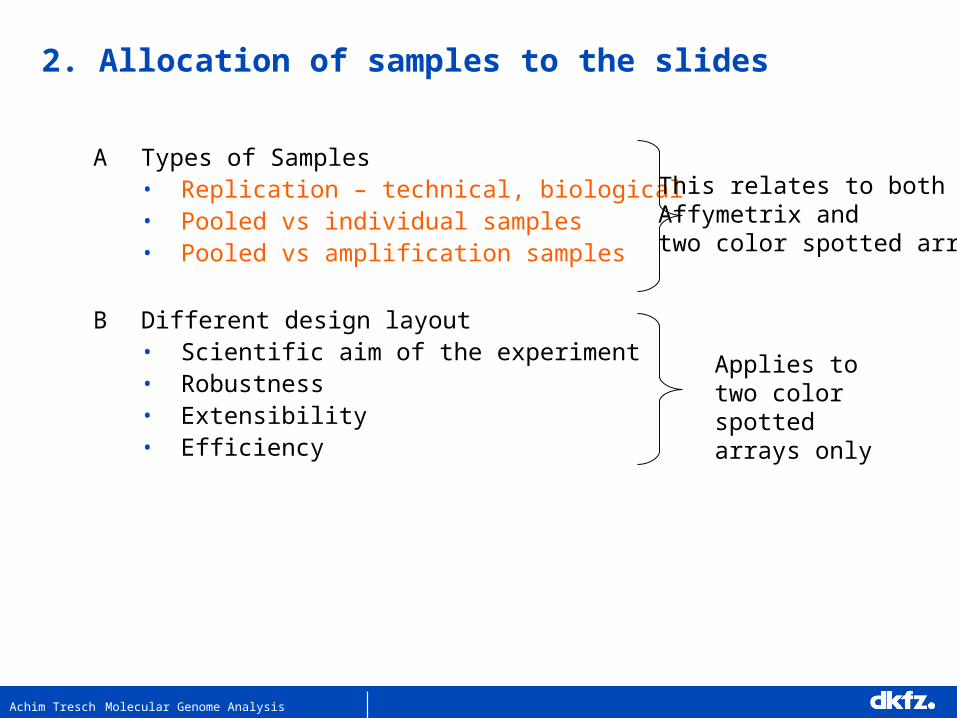
A Types of Samples• Replication – technical, biological• Pooled vs individual samples• Pooled vs amplification samples
B Different design layout • Scientific aim of the experiment• Robustness• Extensibility• Efficiency
2. Allocation of samples to the slides
This relates to bothAffymetrix and two color spotted arrays
Applies to two color spotted arrays only

Achim Tresch Molecular Genome Analysis
Preparing mRNA samples:
Mouse modelDissection of
tissue
RNA Isolation
Amplification
Probelabelling
Hybridization

Achim Tresch Molecular Genome Analysis
Mouse modelDissection of
tissue
RNA Isolation
Amplification
Probelabelling
Hybridization
Biological Replicates
Preparing mRNA samples:

Achim Tresch Molecular Genome Analysis
Mouse modelDissection of
tissue
RNA Isolation
Amplification
Probelabelling
Hybridization
Technical replicates
Preparing mRNA samples:

Achim Tresch Molecular Genome Analysis
Pooling: looking at very small amount of tissues
Mouse modelDissection of
tissue
RNA Isolation
Pooling
Probelabelling
Hybridization

Achim Tresch Molecular Genome Analysis
Design 1
Design 2
Pooled vs Individual samples
Taken from Kendziorski etl al (2003)
Bottleneck: Not enough chips available

Achim Tresch Molecular Genome Analysis
Pooled versus Individual samples
Pooling is seen as “biological averaging”.
Trade off between• Cost of performing a hybridization.• Cost of the mRNA samples.
• Case 1: Cost or mRNA samples << Cost per hybridization
Pooling can assist reducing the number of hybridizations.• Case 2: Cost or mRNA samples >> Cost per hybridization
Hybridize every sample on an individual array to get the maximum amount of information.

Achim Tresch Molecular Genome Analysis
amplification
amplification
Original samples Amplified samples
amplification
amplification
pooling
pooling
Design A
Design B
Amplification vs. Pooling
Bottleneck: Not enough mRNA available

Achim Tresch Molecular Genome Analysis
Pooled vs Amplified samples
• In the cases where we do not have enough material from one biological sample to perform one array (chip) hybridizations, pooling or amplification are necessary.
• Amplification • Introduces more noise.• Non-linear amplification (??), different genes amplified at different rate.• Enables to perform more hybridizations.
• Pooling• Increased effort to obtain sufficiently large number of samples

Achim Tresch Molecular Genome Analysis
A Types of Samples• Replication – technical, biological • Pooled vs individual samples• Pooled vs amplification samples
B Different design layout • Scientific aim of the experiment• Robustness• Extensibility• Efficiency
2. Allocation of samples to the slides
Achim Tresch Molecular Genome Analysis
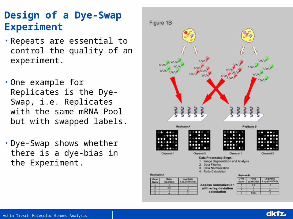
Design of a Dye-Swap Experiment• Repeats are essential to control
the quality of an experiment.
• One example for Replicates is the Dye-Swap, i.e. Replicates with the same mRNA Pool but with swapped labels.
• Dye-Swap shows whether there is a dye-bias in the Experiment.

Achim Tresch Molecular Genome Analysis
Graphical representation
Vertices: mRNA samples;Edges: hybridization;Direction: dye assignment.
Cy3 sample
Cy5 sample

Achim Tresch Molecular Genome Analysis
• The structure of the graph determines which effects can be estimated and
the precision of the estimates.
• Two mRNA samples can be compared only if there is a path joining the
corresponding two vertices.
• The precision of the estimated contrast then depends on the number of
paths joining the two vertices and is inversely related to the length of
the paths.
• Direct comparisons within slides yield more precise estimates than
indirect ones between slides.
Graphical representation

Achim Tresch Molecular Genome Analysis
The simplest design question:Direct versus indirect comparisons
Two samples (A vs B)
e.g. KO vs. WT or mutant vs. WT
A BA
BR
Direct Indirect
2 /2 22
(log (A/B) + log(B/A)) / 2 log (A / R) – log (B / R )
These calculations assume independence of replicates: the reality is not so simple.

Achim Tresch Molecular Genome Analysis
Direct vs Indirect - revisited
A BA
BR
Direct Indirect
y = (a – b) + (a’ – b’)
Var(y/2) = 2 /2 +
y = (a – r) - (b – r’)
Var(y) = 22 - 2
Two samples (A vs B)
e.g. KO vs. WT or mutant vs. WT
2/2 = efficiency ratio (Indirect / Direct) = 1 = 0 efficiency ratio (Indirect / Direct) = 4
= Correlation of replicates

Achim Tresch Molecular Genome Analysis
Experimental results
• 5 sets of experiments with similar structure.
• Compare (Y axis)
Direct) StdErr for aveMmt
Indirect) StdErr for aveMmt – aveMwt
• Theoretical ratio of (A / B) is 1.6
• Experimental observation is 1.1 to 1.4.
SE

Achim Tresch Molecular Genome Analysis
Experimental design• Create highly correlated reference samples to overcome inefficiency in
common reference design.
• Not advocating the use of technical replicates in place of biological replicates for samples of interest.
• Efficiency can be measured in terms of different quantities• number of slides or hybridizations;• units of biological material, e.g. amount of mRNA for one channel.
• In addition to experimental constraints, design decisions should be guided by the knowledge of which effects are of greater interest to the investigator.
E.g. which main effects, which interactions.
• The experimenter should thus decide on the comparisons for which he wants the most precision and these should be made within slides to the extent possible.

Achim Tresch Molecular Genome Analysis
L P
A
w
LPA
w
LPA
22 22
Efficiency rate (Design I(b) / Design II) = 1.5
I (a) Common reference I (b) Common reference II Direct comparison
Number of Slides N = 3 N=6 N=6
mean Variance 2 1 0.67
used Material A = P = L = 1 A = P = L = 2 A = P = L = 2
Experimental design
2 2
2

Achim Tresch Molecular Genome Analysis
Common reference design
• Experiment for which the common reference design is appropriateMeaningful biological control (C) Identify genes that responded differently / similarly across two or more treatments relative to control.
Large scale comparison. To discover tumor subtypes when you have many different tumor samples.
• Advantages:Ease of interpretation.Robustness against failure of microarraysExtensibility - extend current study or to compare the results from current study to other array projects.
T1
Ref
T2 Tn-1 Tn
Achim Tresch Molecular Genome Analysis
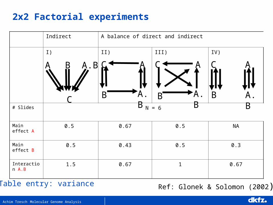
Indirect A balance of direct and indirect
I) II) III) IV)
# Slides N = 6
Main effect A 0.5 0.67 0.5 NA
Main effect B 0.5 0.43 0.5 0.3
Interaction A.B
1.5 0.67 1 0.67
C
A.BBA
B
C
A.B
A
B
C
A.B
A
B
C
A.B
A
Table entry: variance Ref: Glonek & Solomon (2002)
2x2 Factorial experiments
Achim Tresch Molecular Genome Analysis
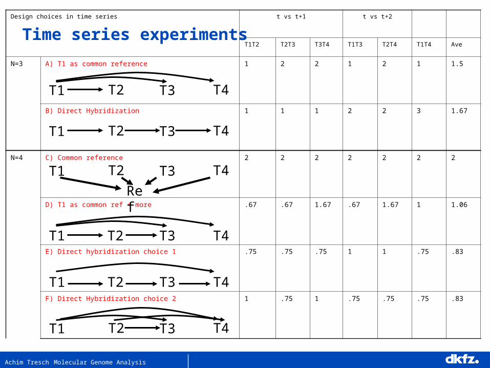
Design choices in time series t vs t+1 t vs t+2
T1T2 T2T3 T3T4 T1T3 T2T4 T1T4 Ave
N=3 A) T1 as common reference 1 2 2 1 2 1 1.5
B) Direct Hybridization 1 1 1 2 2 3 1.67
N=4 C) Common reference 2 2 2 2 2 2 2
D) T1 as common ref + more .67 .67 1.67 .67 1.67 1 1.06
E) Direct hybridization choice 1 .75 .75 .75 1 1 .75 .83
F) Direct Hybridization choice 2 1 .75 1 .75 .75 .75 .83
T2 T3 T4T1
T2 T3 T4T1
Ref
T2 T3 T4T1
T2 T3 T4T1
T2 T3 T4T1
T2 T3 T4T1
Time series experiments

Achim Tresch Molecular Genome Analysis
References
• T. P. Speed and Y. H Yang (2002). Direct versus indirect designs for cDNA microarray experiments. Sankhya : The Indian Journal of Statistics, Vol. 64, Series A, Pt. 3, pp 706-720
• Y.H. Yang and T. P. Speed (2003). Design and analysis of comparative microarray Experiments In T. P Speed (ed) Statistical analysis of gene expression microarray data, Chapman & Hall.
• R. Simon, M. D. Radmacher and K. Dobbin (2002). Design of studies using DNA microarrays. Genetic Epidemiology 23:21-36.
• F. Bretz, J. Landgrebe and E. Brunner (2003). Efficient design and analysis of two color factorial microarray experiments. Biostaistics.
• G. Churchill (2003). Fundamentals of experimental design for cDNA microarrays. Nature genetics review 32:490-495.
• G. Smyth, J. Michaud and H. Scott (2003) Use of within-array replicate spots for assessing differential experssion in microarray experiments. Technical Report In WEHI.
• Glonek, G. F. V., and Solomon, P. J. (2002). Factorial and time course designs for cDNA microarray experiments. Technical Report, Department of Applied Mathematics, University of Adelaide. 10/2002
Monday28. December 2005
MGA Molecular Genome Analysis -Bioinformatics and Quantitative Modeling
Affy Chips:
PM versus MM and
summary information

Achim Tresch Molecular Genome Analysis
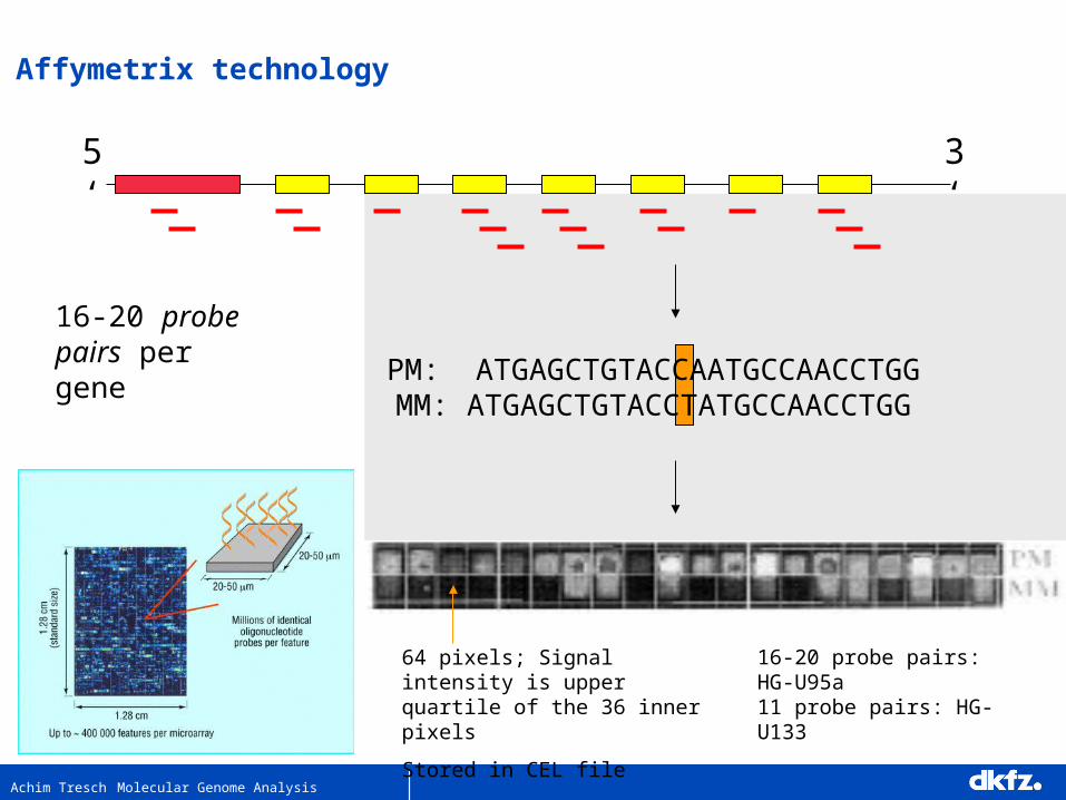
Affymetrix GeneChips: Technical details
24µm24µm
Millions of copies of a specificMillions of copies of a specificoligonucleotide probe oligonucleotide probe synthesized in situ (“grown”)synthesized in situ (“grown”)
Image of Hybridized Probe ArrayImage of Hybridized Probe Array
>200,000 different>200,000 differentcomplementary probes complementary probes
Single stranded, Single stranded, labeled RNA targetlabeled RNA target
Oligonucleotide probeOligonucleotide probe
**
**
*
1.28cm1.28cm
GeneChipGeneChip Probe ArrayProbe ArrayHybridized Probe CellHybridized Probe Cell

Achim Tresch Molecular Genome Analysis
Achim Tresch Molecular Genome Analysis
5‘ 3‘
PM: ATGAGCTGTACCAATGCCAACCTGGMM: ATGAGCTGTACCTATGCCAACCTGG
16-20 probe pairs per gene
16-20 probe pairs: HG-U95a11 probe pairs: HG-U133
64 pixels; Signal intensity is upper quartile of the 36 inner pixels
Stored in CEL file
Affymetrix technology

Achim Tresch Molecular Genome Analysis
Affymetrix expression measures
• PMijg, MMijg = Intensity for perfect match and mismatch
probe j for gene g in chip i.
• i = 1,…, n one to hundreds of chips
• j = 1,…, J usually 16 or 20 probe pairs
• g = 1,…, G 8…20,000 probe sets.
• Tasks:
• calibrate (normalize) the measurements from different chips (samples)
• summarize for each probe set the probe level data, i.e., 20 PM and MM pairs, into a single expression measure.
• compare between chips (samples) for detecting differential expression.

Achim Tresch Molecular Genome Analysis
Low – level -Analysis
• Preprocessing signals: background correction, normalization, PM-
adjustment, summarization.
• Normalization on probe or probe set level?
• Which probes / probe sets used for normalization
• How to treat PM and MM levels?

Achim Tresch Molecular Genome Analysis

Achim Tresch Molecular Genome Analysis

Achim Tresch Molecular Genome Analysis

Achim Tresch Molecular Genome Analysis

Achim Tresch Molecular Genome Analysis
Arguments against the use of d = PM-MM
• Difference is more variable. Is there a gain in bias to compensate for the loss of precision?
• MM detects signal as well as PM
• PM / MM results in a bias.
• Subtraction of MM is not strong enough to remove probe effects, nothing is gained by subtraction

Achim Tresch Molecular Genome Analysis
-2 0 2 4 6 8 10
02
46
81
0
Kontrollpool 1 - transf. Expression
Ko
ntro
llpo
ol 2
- tr
ans
f. E
xpre
ssio
n
MAS5
4 6 8 10 12 14
46
81
01
21
4
Kontrollpool 1 - transf. Expression
Ko
ntro
llpo
ol 2
- tr
ans
f. E
xpre
ssio
n
RMA
Example LPS: Expression Summaries

Achim Tresch Molecular Genome Analysis
How to approach the quantification of gene expression:Three data sets to learn from
• Mouse Data Set (A) 5 MG-U74A GeneChip arrays, 20% of the probe pairs were incorrectly sequenced, measurements read for these probes are entirely due to non-specific binding
• Spike-In Data Set (B) 11 control cRNAs were spiked-in at different concentrations
• Dilution Data Set (C) Human liver tissues were hybridised to HG-U95A in a range of proportions and dilutions.

Achim Tresch Molecular Genome Analysis
Normalization – Baseline Array
Data CRaw PM Raw PM-MM
Normalized PM Normalized PM-MM

Achim Tresch Molecular Genome Analysis
• Graphical tool to evaluate summaries of Affymetrix probe level data.
• Plots and summary statistics
• Comparison of competing expression measures
• Selection of methods suitable for a specific investigation
• Use of benchmark data sets
What makes a good expression measure: leads to good and precise answers to a research question.
AffyComp

Achim Tresch Molecular Genome Analysis
> affycompTable(rma.assessment, mas5.assessment)
RMA MAS.5.0 whatsgood Figure
Median SD 0.08811999 2.920239e-01 0 2
R2 0.99420626 8.890008e-01 1 2
1.25v20 corr 0.93645083 7.297434e-01 1 3
2-fold discrepancy 21.00000000 1.226000e+03 0 3
3-fold discrepancy 0.00000000 3.320000e+02 0 3
Signal detect slope 0.62537111 7.058227e-01 1 4a
Signal detect R2 0.80414899 8.565416e-01 1 4a
Median slope 0.86631340 8.474941e-01 1 4b
AUC (FP<100) 0.82066051 3.557341e-01 1 5a
AFP, call if fc>2 15.84156379 3.108992e+03 0 5a
ATP, call if fc>2 11.97942387 1.281893e+01 16 5a
FC=2, AUC (FP<100) 0.54261364 6.508575e-02 1 5b
FC=2, AFP, call if fc>2 1.00000000 3.072179e+03 0 5b
FC=2, ATP, call if fc>2 1.71428571 3.714286e+00 16 5b
IQR 0.30801579 2.655135e+00 0 6
Obs-intended-fc slope 0.61209902 6.932507e-01 1 6a
Obs-(low)int-fc slope 0.35950904 6.471881e-01 1 6b

Achim Tresch Molecular Genome Analysis
good
badW. Huber
affycomp results (28 Sep 2003)

Achim Tresch Molecular Genome Analysis
Acknowledgements – Slides borrowed from
• Wolfgang Huber
• Ulrich Mansmann
• Terry Speed
• Benedikt Brors
• Anja von Heydebreck
• Tim Beissbarth
• Rainer König

Achim Tresch Molecular Genome Analysis

Monday28. December 2005
MGA Molecular Genome Analysis -Bioinformatics and Quantitative Modeling
Sources of Variation
• Variance and Bias• Different Sources of Variation• Measuring foreground and background signal• Control quality at different levels

Achim Tresch Molecular Genome Analysis
How to create the trapezoid? ROC changing the cutpoint

Achim Tresch Molecular Genome Analysis


