
299 NEW EVIDENCE ON LONG-RUN OUTPUT CONVERGENCE
Journal of Applied Economics. Vol VIII, No. 2 (Nov 2005), 299-319
NEW EVIDENCE ON LONG-RUN OUTPUT CONVERGENCEAMONG LATIN AMERICAN COUNTRIES
MARK J. HOLMES ∗∗∗∗∗
Waikato University Management School
Submitted February 2004; accepted August 2004
This study assesses long-run real per capita output convergence among selected LatinAmerican countries. The empirical investigation, however, is based on an alternativeapproach. Strong convergence is determined on the basis of the first largest principalcomponent, based on income differences with respect to a chosen base country, beingstationary. The qualitative outcome of the test is invariant to the choice of base countryand, compared to alternative multivariate tests for long-run convergence, this methodologyplaces less demands on limited data sets. Using annual data for the period 1960-2000,strong convergence is confirmed for the Central American Common Market. However, anamended version of the test confirms weaker long-run convergence in the case of the LatinAmerican Integration Association countries.
JEL classification codes: F15, O19, O40, O54Key words: output convergence, Latin America, common trends
I. Introduction
In recent years, economists have keenly debated the issue of whether or not
per capita incomes across countries are converging. The neoclassical growth modelpredicts that countries will converge towards their balanced growth paths where
per capita growth is inversely related to the starting level of income per capita.
Early studies by Barro (1991), Barro and Sala-i-Martin (1991,1992), Baumol (1986),Sala-i-Martin (1996) and others that consider convergence across countries, US
states and European regions, argue that in most instances the rate annual rate of
convergence is roughly 2%. This is confirmed by studies such as Mankiw et al.
∗ Department of Economics, Waikato University Management School, Hamilton, New Zealand.Email: [email protected]. I would like to express my gratitude to the co-editorGermán Coloma and three anonymous referees for their very helpful comments. Any remainingerrors are my own.

JOURNAL OF APPLIED ECONOMICS300
(1992) who investigate conditional convergence that allows for population growthand capital accumulation. More recent studies have offered mixed evidence on
this question. For instance, Quah (1996) questions the 2% convergence rate and
argues that convergence will take place within relatively homogenous convergenceclubs. McCoskey (2002) suggests that convergence clubs and regional
homogeneity is probably unresolved with respect to less developed countries
(LDCs) where geographic proximity and cross-national economic interdependencewill cause groups of LDCs to grow or falter as one. As noted by Dobson and
Ramlogan (2002), little is known about the convergence process among LDCs and
the limited range of studies that have considered LDCs have proceeded at a highlyaggregated level (Khan and Kumar 1993) or have focused on convergence within
a particular country (Ferreira 2000, Nagaraj et al. 2000, Choi and Li 2000). The
purpose of this paper is to examine convergence among Latin American countrieswhere we assess the possibility of convergence clubs within LDCs based on
common characteristics regarding international trade arrangements.
The recent study by Dobson and Ramlogan (2002) investigates convergenceamong Latin American countries over the study period 1960-90. They find evidence
of unconditional beta convergence (poor countries growing faster than richer
countries towards a common steady state) but not sigma convergence (distributionof income becoming more equal) across the full study period. However, by looking
at sub-periods, they find that the rates of conditional convergence towards
individual steady states are highest during the 1970s-mid 1980s. In addition tothis, Dobson and Ramlogan conclude that the estimates of convergence may be
sensitive to how GDP is measured.
The question of whether trade liberalization is associated with incomeconvergence remains unresolved both in terms of theory and evidence.1 Using
annual data on real per capita GDP for a total sample of sixteen Latin American
countries,2 this study offers an empirical assessment of whether long-run incomeconvergence among LDCs has been achieved by countries that have participated
in the Latin American Integration Association (LAIA) and Central American
Common Market (CACM). The LAIA was formed in 1980 by Argentina, Bolivia,Brazil, Chile, Colombia, Ecuador, Mexico, Paraguay, Peru, Uruguay, and Venezuela,
1 See, for example, Slaughter (2001) and references therein.
2 The full list of countries includes Argentina, Bolivia, Brazil, Chile, Colombia, Costa Rica,Ecuador, El Salvador, Guatemala, Honduras, Mexico, Nicaragua, Paraguay, Peru, Uruguay andVenezuela.

301 NEW EVIDENCE ON LONG-RUN OUTPUT CONVERGENCE
taking over the duties of the Latin American Free Trade Association (LAFTA),
which had been created in 1960 to establish a common market for its member
nations through progressive tariff reductions until the elimination of tariff barriers
by 1973. In 1969 the deadline was extended until 1980, at which time the plan was
scrapped and the new organization, the LAIA, was created by the Treaty of
Montevideo. It has the more limited goal of encouraging free trade, with no deadline
for the institution of a common market. Economic hardship in Argentina, Brazil,
and many other member nations has made LAIA’s task difficult. The CACM was
created in 1960 by a treaty between Guatemala, Honduras, Nicaragua, El Salvador,
and later Costa Rica. By the mid-1960s the group had made advances toward
economic integration, and by 1970 trade between member nations had increased
more than tenfold over 1960 levels. During the same period, imports doubled and
a common tariff was established for 98% of the trade with non-member countries.
In 1967, it was decided that CACM, together with the Latin American Free Trade
Association, would be the basis for a comprehensive Latin American common
market. However, by the early 1990s little progress toward a Latin American common
market had been made, in part because of internal and internecine strife, and in part
because CACM economies were competitive, not complementary. Nonetheless,
the CACM with a stronger focus on creating a common market than the LAIA, has
been judged more successful at lowering trade barriers than other Latin American
groupings.
While this study is motivated by the desire to throw more light on the issue of
convergence among LDCs, there are further reasons of interest attached to this
study. First, a key contribution is in terms of the methodology employed. The tests
for income convergence are on the basis of whether the largest principal component,
based on benchmark deviations from base country output, is stationary or not.
This methodology, initially advocated by Snell (1996), offers a number of advantages
over existing tests for convergence. Unlike the estimation of bivariate equations,
the outcome of this test for convergence is not critically dependent on the choice
of base country. Also, there are advantages over alternative common trends
methods based on Johansen (1988) and Stock and Watson (1988), which can
suffer from low test power on account of data limitations, as well as principal
components analyses that search for integration using arbitrary methods to
determine the ‘significance’ of given components. Second, the concept of
convergence in the context of the groupings we analyze is important. Essentially,
this study tests the hypothesis that convergence is a phenomenon where experience

JOURNAL OF APPLIED ECONOMICS302
as trading partners or geographical location has the potential to bind economies
together. Given that these agreements have sought to promote integration as part
of their long-term objectives, the absence of convergence would justify the need
for proactive policies to promote growth and reduce income inequalities. If one
finds that the incomes of countries within these groups have converged, then it
becomes more difficult to justify regional development policy in terms of economic
efficiency (Dobson and Ramlogan 2002). Third, the concept of convergence
employed in this study differs from that employed by Barro, Sala-i-Martin and
others. These studies define convergence with respect to poorer countries growing
faster than richer countries towards some (common or individual) steady state.
The notion of convergence employed in this study is based on testing whether per
capita outputs move together over time with no tendency to drift further apart in
the long-run following a deviation from equilibrium.
The paper is organized as follows. The following section briefly considers the
literature on trade liberalization and income convergence. The groupings of
countries used in this study are then outlined. Section III discusses the data and
econometric methodology. This leads to a new categorization of types of real
convergence based on the stationarity of the first largest principal component.
Section IV reports and discusses the results. The evidence suggests that long-run
convergence is strongest among the CACM for whom the first largest principal
component is stationary. On the other hand, the LAIA countries are weakly
convergent. Section V concludes.
II. Trade, convergence and international agreements
The traditional approach to the convergence debate concerns poor countries
catching up with rich ones. In the approaches taken by studies such as Barro
(1991), Barro and Sala-i-Martin (1991,1992), Baumol (1986) and Sala-i-Martin (1996),
a cross-section of growth rates are regressed on income levels and the estimated
coefficient informs on the rate at which poor countries catch up with those richer.
Quah (1996) argues that the conventional analyses miss key aspects of growth
and convergence. Moreover, it is argued that the key issue is what happens to the
cross-sectional distribution of economies, not whether an economy tends towards
its own steady state. Quah therefore considers issues of persistence and
stratification in the context of convergence clubs forming where the cross-section
polarizes into twin peaks of rich and poor. The economic forces that drive this
303 NEW EVIDENCE ON LONG-RUN OUTPUT CONVERGENCE
notion of convergence include factors such as capital market imperfections, countrysize, club formation, etc.
Structural and institutional factors are crucial in forming the background against
which long-run linkages between countries can exist. As pointed out by Slaughter(2001), many papers on convergence cannot analyze the role of international trade
because they assume a ‘Solow world’ in which countries produce a single aggregate
good independently of each other. Moreover, convergence arises from capitalstock convergence. However, trade theory that draws on and develops some of
the arguments belonging to the factor price equalization theorem, Heckscher-Ohlin
models, Stolper-Samuelson effects or Rybczynski theorem offers an ambiguousprediction as to whether or not trade liberalization will cause per capita incomes to
converge or diverge. The convergence of factor prices via the factor price equilibrium
theorem depends on cross-country tastes, technology and endowments. It is arguedthat trade liberalization has an ambiguous effect on endowments of labor and
capital (see, for example, Findlay 1984). Trade liberalization may reduce investment
risk particularly in poorer countries (see, for example, Lane 1997). Divergence mayoccur through the Stolper-Samuelson effects of liberalization on capital rentals
where Baldwin (1992) argues that dynamic gains from trade will mean that richer
countries that are well endowed with capital will experience increased capital rentals.Ventura (1997) argues that free trade may inhibit the onset of diminishing returns
to investment where richer countries do not lose their incentive to invest as they
would under autarky. Finally, income convergence will be affected by technologyflows. Matsuyama (1996) argues that freer trade leads poorer countries to specialize
in technologically-stagnant products because they lack the resources to engage
in the production of high-technology products.Empirical evidence on trade and income convergence is also mixed. Ben-David
(1993, 1996) and Sachs and Warner (1995) find that international trade causes
convergence. Sachs and Warner point to the convergence club of economieslinked by international trade. Ben-David (1996) finds that it is the wealthier countries
that trade significantly who are characterized by per capita convergence. Ben-
David (1993) analyses five episodes of post-1945 trade liberalization and finds thatincome convergence generally shrank after liberalization started. On the other
hand, Bernard and Jones (1996) find that freer trade causes incomes to diverge
while Slaughter (2001), using a sample of developed countries and LDCs, finds nostrong, systematic link between trade liberalization and convergence. Indeed,
Slaughter suggests that much of the evidence indicates that trade liberalization
diverges incomes among the liberalizers.
JOURNAL OF APPLIED ECONOMICS304
III. Data and methodology
This study employs data for annual per capita real GDP (US$) for each of the
sample of countries for study periods of 1960 up to 2000. All data are obtained fromthe Penn World Tables version 6.1. The following study periods are considered:
the full study period of 1960-2000, 1981-2000 which represents the period of
operation for the LAIA3, and 1960-1980 to analyse convergence among the LAIAcountries before their agreement became operational. As well as examining
groupings based on the CACM and LAIA countries, this study also considers the
full sample of countries taken together (All) as well as groupings based ongeographical location within Latin America namely, Colombia, Costa Rica, Ecuador,
El Salvador, Guatemala, Honduras, Mexico, Nicaragua and Venezuela (North) along
with Argentina, Bolivia, Brazil, Chile, Paraguay, Peru and Uruguay (South). Theexclusion of certain countries from some of the groups is driven by data availability
over the full study period. Using this data, this study employs a two-stage testing
procedure for income convergence. The first stage draws on a technique, developedby Snell (1996), which is an extension of the principal components methodology,
based on testing for the stationarity of the first largest principal component (LPC)
of benchmark deviations from base country output for each group in turn. Thistest can confirm long-run convergence where all series move in tandem over the
long-run. This can be described as strong convergence. The second stage applies
if stage one finds against strong convergence. Principal components are computedfor each group where per capita incomes are expressed in levels rather than
differences from base country and the number of common shared trends are
calculated. This second stage searches for evidence of a single common sharedtrend driving the output series. This would confirm weak convergence because,
unlike stage one, homogeneity between the countries has been relaxed.
With regard to the first stage of the convergence test, suppose n + 1 countriesconstitute the sample of a given group. The benchmark deviations are defined as
where yit and y
Gt respectively denote the natural logarithm of the real per capita
income of country i and the chosen base-country, and i = 1, 2,…, n. Let Xt be an
3 The LAIA study period covers 1981-2000 because the 1980 Treaty of Montevideo became
operational in 1981.
,)( ittGi uyy =− (1)

305 NEW EVIDENCE ON LONG-RUN OUTPUT CONVERGENCE
(nx1) vector of random variables, namely the uit’s for each of the n countries, which
may be integrated up to order one. The principal components technique addresses
the question of how much interdependence there is in the n variables contained in
Xt. We can construct n linearly independent principal components which collectively
explain all of the variation in Xt where each component is itself a linear combination
of the uit’s.4 Since I(1) variables have infinite variances, whereas stationary, I(0),
variables have constant variances, it follows that the first LPC, which explains thelargest share of the variation in X
t, is the most likely to be I(1) and so corresponds
to the notion of a common trend (Stock and Watson 1988). However, if the first LPC
is I(0) then all the remaining principal components will also be stationary and thereare no common trends which suggests that the u
it’s contained in X
t are themselves
stationary. This will confirm real convergence with the base-country across the
sample of n benchmark deviations.More formally, following Stock and Watson (1988) we can argue that each
element of Xt may be written as a linear combination of k ≤ n independent common
trends which are I(1), and (n – k) stationary components which correspond to theset of (n – k) cointegrating vectors among the u
it’s. The k vector of common trends
and (n – k)x1 vector of stationary components may respectively be written as
where α is an (n – k) matrix of full column rank, β is an nx(n – k) matrix that forms the(n – k) cointegrating vectors, α’α = I and α’β = 0. If there are k common trends, it
can be shown that the k LPCs of Xt may be written as
where *tX is a vector of observations on the u
it’s in mean deviation form, α*
represents the k eigenvectors corresponding to the largest eigenvalues of Xt and
is defined as αR where R is an arbitrary, orthogonal (kxk) matrix of full rank. Thisrelationship guarantees that under the null hypothesis of k common trends, each
of the k LPC’s will be I(1). Similarly, for the (n – k) remaining principal components,
it can be shown that
4 See, for example, Child (1970).
,tt Xατ ′= (2)
,tt Xβξ ′= (3)
,*** ατ′
= tt X (4)

JOURNAL OF APPLIED ECONOMICS306
where β* corresponds to the (n – k) eigenvectors that provide the (n – k) smallestprincipal components and is defined as βS where S is an arbitrary orthogonal (n –k)x(n-k) matrix.
The first LPC will be I(1) provided there is at least one common trend among theu
it’s contained in X
t. We can therefore test the null hypothesis that the first LPC is
non-stationary against the alternative hypothesis that the first LPC is I(0). Rejectionof the null means that all principal components are stationary and so there are nocommon trends among the u
it’s contained in X
t. This confirms convergence with
respect to the base-country across the sample. To test the stationarity of the firstLPC we can use the familiar Augmented Dickey-Fuller (ADF) test based on
where the first LPC is calculated as **11 tXz α= using *
1α as the first column of α*,and e
t is a white noise error term. If we find that z
1 is trend stationary only, this will
not confirm convergence because for at least one series in the sample, the differencefrom base country is growing over time. This would imply the presence of at leasttwo common shared trends among the X
t ‘s.
This notion of convergence can be seen in the context of the Bernard andDurlauf (1995) definition of convergence in a stochastic environment where thelong-run forecasts of the benchmark deviations tend to zero as the forecast horizontends to infinity. If each y is I(1) or first difference stationary, then convergenceimplies that each ittGi uyy =− )( is a stationary process (since the per capitaincome series are indices having different bases, we may allow the benchmarkdeviations to have different means) where each y
it and y
Gt is cointegrated with a
cointegrating vector [1, -1].An alternative way forward is to test for a single common trend among a series
of I(1) variables ),,....,,( 21 Gtnttt yyyy where convergence is confirmed throughthe presence of n cointegrating vectors among the n + 1 countries. The advantageof examining the stationarity of the first LPC is that, unlike the Johansen (1988)maximum likelihood procedure (and the Stock and Watson 1988 common trendframework), it does not require the estimation of a complete vector autoregressionsystem (VAR).5 The size and power of this test is not affected by the VAR being
,*** βξ′
= tt X (5)
,1
1111 t
p
iittt ezzz +∆+=∆ ∑
=−− γρ (6)
5 See, for example, Mills and Holmes (1999) who employ these methods to examine commontrends among European output series during the Bretton Woods and Exchange Rate Mechanismeras.

307 NEW EVIDENCE ON LONG-RUN OUTPUT CONVERGENCE
constrained to an unreasonably low order on account of data limitations. Thismethod also avoids the need for an entire sequence of tests for the stationarity of
a multivariate system. As indicated by Snell, even if each test in the sequence had
a reasonable chance of rejecting the false null, the procedure as a whole is likely tohave low power. Another important issue is whether the choice of base country
affects the outcome of the test. This methodology employed in this paper is based
on a multivariate test for convergence that is not critically dependent upon thechoice of base country. In one scenario we may find that the first LPC constructed
from the n income differentials is stationary thereby suggesting that all n + 1countries in the sample share the same common stochastic trend. It will not matterwhich country is used as base because the first LPC will still be stationary. If the
first LPC is non-stationary, then there are at least two common stochastic trends
among the sample of n + 1 countries with a maximum of n countries sharing thesame trend. In this case, it is impossible to change to base country so that the first
LPC is stationary.
The second stage of the test is applied if one is unable to reject the null that thefirst LPC based on differences with respect to base country is non-stationary. So
far, under the LPC test, income differentials are constructed among the lines of( )tGii yy β− where .1 ii ∀=β Since the differentials are computed as (y
i – y
G)
t, this
means that homogeneity has been imposed, i.e., ,1 ii ∀=β before the test is
conducted. Strong convergence, which is based on homogeneity, is therefore
confirmed if the first LPC is stationary. Non-stationarity of the first LPC may occurbecause β
i ≠ 1 in at least one case. Even if y
i and y
G are cointegrated, it may now be
more appropriate to think of the long-run cointegrating relationship not being
written as itGtit uyy += but rather as itGtiit uyy += β instead. In the latter case,homogeneity has not been imposed and it is weak convergence that is being
tested for where the variables used to construct the principal components are
Gn yyy ,,,.........1 instead of ( ) iGi uyy =− for .,.....,1 ni = Moreover, it is possiblethat the y series are driven by a single common shared trend but without the
homogeneity that strong long-run convergence implies.
To address the possibility of weak convergence, principal components arecomputed for the n + 1 countries expressed in levels rather than differences with
respect to a base country. If the first and second LPCs are respectively non-
stationary and stationary, this will suggest there are n cointegrating vectors presentand therefore one ((n + 1) – n = 1) common shared trend. We can describe this as
weak convergence because the first stage of the test described previously did not
support convergence based on homogeneity, yet the second stage of the test

found that the countries are nonetheless sharing the same long-run trend.6Wemay find that the third LPC is the first principal component that is stationary. In
this case, we have n − 1 cointegrating vectors present and this implies the presence
of two ((n + 1) – (n - 1) = 2) common trends among the n + 1 countries. This is yetweaker evidence of convergence. In the extreme, we may find that none of the
principal components are stationary. This implies that there are no cointegrating
vectors and therefore n + 1 common trends and the sample of n + 1 countries. Thiswould be consistent with zero long-run convergence or complete divergence.
Before proceeding to the results discussion, it is important to highlight some
caveats associated with this methodology. The advantages over existing methodsof testing for long-run convergence have been discussed, however the downside
of this methodology concerns a standard criticism of principal component
estimation and indeed of common stochastic trends. They are linear combinationsof economic variables and so the economic interpretation of a given component
can be problematic. Also, testing the null of non-stationarity of the first LPC
leaves one vulnerable to the standard criticisms concerning the low power attachedto unit root tests making it difficult to reject the null of non-stationarity. A final
caveat concerns a situation where there exist two or more common trends under
the null hypothesis. The ADF unit root test is conducted on the series with thelargest sum of squares. However, if we take equation (6), the simple Dickey-Fuller
statistic is asymptotically proportional to ( ) .5.02
11 ∑∑ −− ttt zez It is possible
that the size of the test under such a null may actually be less than 5%.
IV. Results
Before proceeding to the LPC-based tests, we may first consider the traditional
test for absolute beta convergence among Latin American countries. Using thedata set, the following result was obtained using OLS for the full sample of sixteen
Latin American countries across the study period 1960-2000:
6 If first LPC is stationary, this will imply that all real per capita incomes within the sample arestationary. Although there are no common trends among the n + 1 countries, this result wouldat least imply non-divergence among the series. As is seen later, this particular state of affairs
is precluded by the unit root tests.
( ) ( )006.0 0.047
,004.0041.0 ,,,, titiTtti y εγ +−=+(7)
JOURNAL OF APPLIED ECONOMICS308

where γ is the annualised growth rate of per capita GDP over T time periods, yt is
the initial level of per capita GDP of country i and standard errors are reported in
parentheses. While the negative slope conforms to the priors suggested by the
traditional approach, it is insignificantly different from zero. Thus using traditionalconvergence tests applied to this data set yields results that are not supportive of
convergence.
Table 1. DFGLS unit root tests on per capita income
1960-2000 1981-2000
No trend Trend No trend Trend
Argentina LAIA -1.174 -2.327 -0.945 -1.877
Bolivia LAIA -1.847 * -2.286 -0.496 -0.658
Brazil LAIA 0.916 -0.961 -0.614 -3.670***
Chile LAIA 1.537 -1.198 -0.268 -1.555
Columbia LAIA -0.174 -1.450 -1.222 -2.293
Costa Rica CACM -0.557 -1.316 -0.671 -1.107
Ecuador LAIA -0.373 -0.339 -0.260 -2.073
El Salvador CACM -0.564 -2.394 -0.763 -1.328
Guatemala CACM 0.020 -1.214 -1.460 -1.465
Honduras CACM -0.624 -0.987 -0.540 -3.103* *
Mexico LAIA 1.057 -1.060 -0.690 -0.862
Nicaragua CACM 0.140 -1.171 0.479 -1.509
Paraguay LAIA -1.097 -2.065 -0.954 -1.057
Peru LAIA -0.656 -1.287 -1.507 -2.153
Uruguay LAIA 0.414 -1.695 -1.570 -1.904
Venezuela LAIA -0.415 -1.587 -0.412 -1.876
Note: These are DFGLS unit root tests advocated by Elliot, Rothenberg and Stock (1996). Inall cases, the lag lengths are selected on the basis of the Akaike Information Criteria (AIC).Excluding a trend, *** , ** and * indicate rejection of the null of non-stationarity the 1, 5 and10% levels using critical values of -2.58, -1.95 and -1.62 respectively. Including a trend, the 1,5 and 10% critical values used are -3.48, -2.89, -2.57 respectively.
Country Group
In the search for long-run relationships among the real per capita incomesusing the alternative LPC-based approach, we first require that the series are non-
stationary. An important issue to consider is whether or not the use of transformed
data by means of natural logarithms is appropriate. For this purpose, the serieswere subjected to a range of tests advocated by Franses and McAleer (1998)
309 NEW EVIDENCE ON LONG-RUN OUTPUT CONVERGENCE
JOURNAL OF APPLIED ECONOMICS310
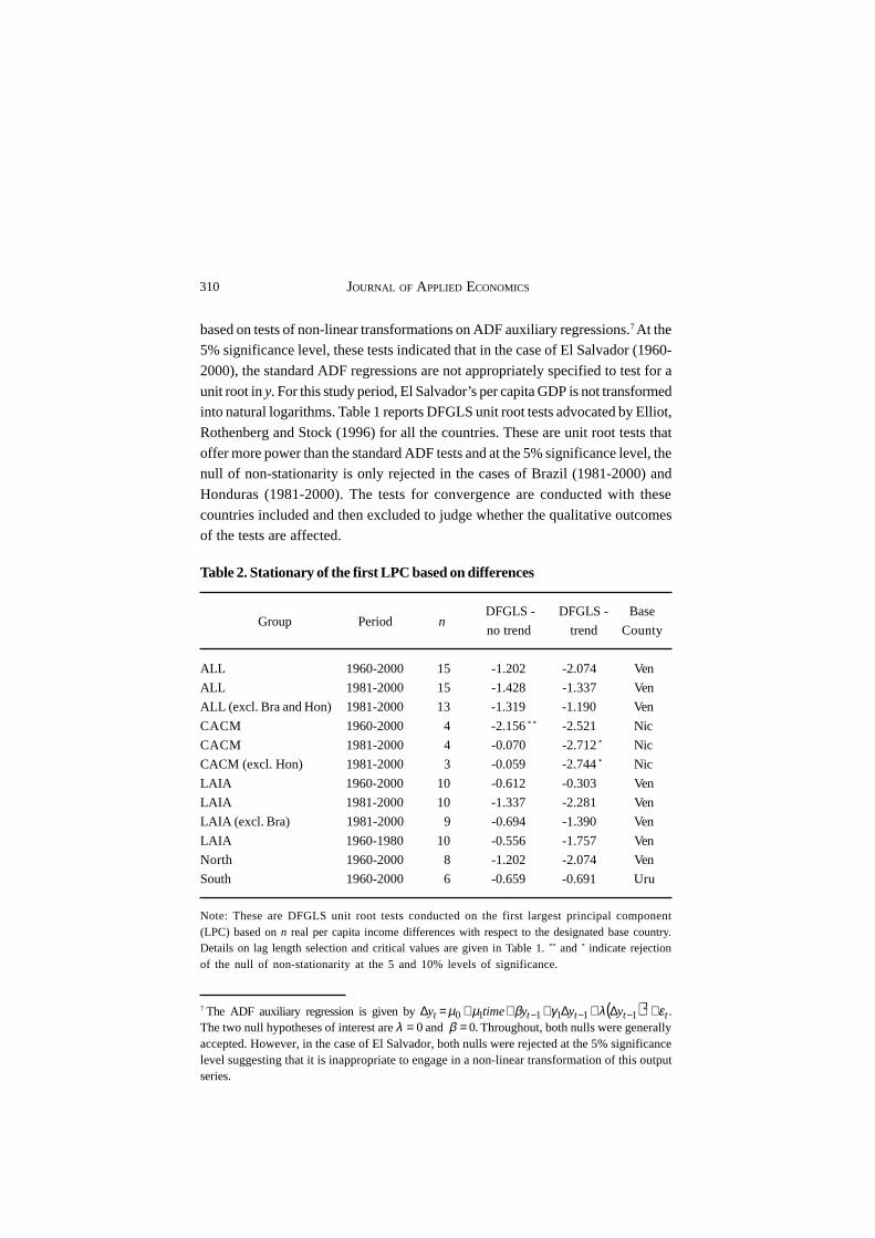
based on tests of non-linear transformations on ADF auxiliary regressions.7 At the5% significance level, these tests indicated that in the case of El Salvador (1960-
2000), the standard ADF regressions are not appropriately specified to test for a
unit root in y. For this study period, El Salvador’s per capita GDP is not transformedinto natural logarithms. Table 1 reports DFGLS unit root tests advocated by Elliot,
Rothenberg and Stock (1996) for all the countries. These are unit root tests that
offer more power than the standard ADF tests and at the 5% significance level, thenull of non-stationarity is only rejected in the cases of Brazil (1981-2000) and
Honduras (1981-2000). The tests for convergence are conducted with these
countries included and then excluded to judge whether the qualitative outcomesof the tests are affected.
7 The ADF auxiliary regression is given byThe two null hypotheses of interest are 0=λ and .0=β Throughout, both nulls were generallyaccepted. However, in the case of El Salvador, both nulls were rejected at the 5% significancelevel suggesting that it is inappropriate to engage in a non-linear transformation of this outputseries.
( ) .2111110 ttttt yyytimey ελγβµµ +∆+∆+++=∆ −−−
Table 2. Stationary of the first LPC based on differences
DFGLS - DFGLS - Base
no trend trend County
ALL 1960-2000 15 -1.202 -2.074 Ven
ALL 1981-2000 15 -1.428 -1.337 Ven
ALL (excl. Bra and Hon) 1981-2000 13 -1.319 -1.190 Ven
CACM 1960-2000 4 -2.156* * -2.521 Nic
CACM 1981-2000 4 -0.070 -2.712* Nic
CACM (excl. Hon) 1981-2000 3 -0.059 -2.744* Nic
LAIA 1960-2000 10 -0.612 -0.303 Ven
LAIA 1981-2000 10 -1.337 -2.281 Ven
LAIA (excl. Bra) 1981-2000 9 -0.694 -1.390 Ven
LAIA 1960-1980 10 -0.556 -1.757 Ven
North 1960-2000 8 -1.202 -2.074 Ven
South 1960-2000 6 -0.659 -0.691 Uru
Note: These are DFGLS unit root tests conducted on the first largest principal component(LPC) based on n real per capita income differences with respect to the designated base country.Details on lag length selection and critical values are given in Table 1. ** and * indicate rejectionof the null of non-stationarity at the 5 and 10% levels of significance.
Group Period n

311 NEW EVIDENCE ON LONG-RUN OUTPUT CONVERGENCE
The first stage of the convergence test is to take each of the three groupingsand express per capita income with respect to a chosen base country. The choice
of base countries includes Venezuela for the LAIA countries, Nicaragua for the
CACM countries and Venezuela for the grouping that comprises all countries.Table 2 reports that in all cases except the CACM countries, the null of non-
stationarity of the first LPC is accepted at the 10% significance level. Strong
convergence with homogeneity is generally rejected for the LAIA and indeed, allLatin American countries and we are therefore unable to conclude that the movement
in LDC per capita income levels are characterized as being convergent in the long-
run with a coefficient of unity. This evidence of non-convergence also applies tothe LAIA countries prior to 1981 (1960-80) as well as the geographical groupings
based on North and South.
Table 3. Stationary of the LPCs based on real per capita income levels
DFGLS - DFGLS -
no trend trend
ALL 1960-2000 16 3 -2.021* * -2.578* 2
ALL 1981-2000 16 5 -2.984*** -2.784* 4
ALL (excl. Bra and Hon) 1981-2000 14 4 -3.213*** -3.262* * 3
LAIA 1960-2000 11 5 -2.009* * -2.747* 4
LAIA 1981-2000 11 2 0.280 -3.244* * 1
LAIA (excl. Bra) 1981-2000 10 2 0.280 -3.268* * 1
LAIA 1960-1980 11 3 -2.025* * -2.231 2
North 1960-2000 9 3 -2.039* * -2.618* * 2
South 1960-2000 7 5 -3.119*** -4.096*** 4
Note: The column headed n+1 refers to the number of countries. The column headed LPCindicates which LPC is the first that is identified as being stationary according to the DFGLSunit root tests. Details on lag length selection and critical values are given in Table 1. *** , ** and* indicate rejection of the null of non-stationarity at the 1, 5 and 10% levels of significancerespectively in the unit root tests. The column headed k indicates the number of commonshared trends present for each group.
Group Period n+1 LPC k
The second stage of the convergence test applies to those groups for whom
the first LPC was non-stationary. This second test is based on the search for a
single common trend among the series in levels form rather than differences with
respect to base country. The results reported in Table 3 suggest that it is only in

JOURNAL OF APPLIED ECONOMICS312
the case of the LAIA countries (1981-2000) that a single common trend is confirmedwhere the second LPC is the first principal component that is stationary. However,
since the first stage of the test found against strong convergence, we conclude
that homogeneity with respect to long-run movements in income levels is notpresent here and so the LAIA group is characterized as being weakly convergent.
However, this evidence of weak convergence for the LAIA countries does not
extend across the full study period of 1960-2000 where four single common trendsare present among the eleven LAIA countries,8or over the sub-period 1960-1980
where two common trends are present. Evidence of multiple common shared trends
is also present in the case of all the Latin American countries together as well asthe geographical groupings based on North and South. Overall, the firmest evidence
in favor of weak convergence in Table 3 is associated with the LAIA countries
during the period 1981-2000 since the consideration of alternative groups andalternative sub-periods points towards the presence of multiple common trends.
These latter findings are in principle consistent with Dobson and Ramlogan (2002)
who do not find convincing evidence in favor of sigma convergence for their1960-90 study period of Latin American countries.
The results reported in Tables 2 and 3 indicate that evidence of convergence is
strongest in the case of the CACM rather than LAIA. It should be rememberedthat many Latin American economies have experienced serious turbulence during
the study period.9 It is therefore pertinent to ask whether the results obtained for
the LAIA in Tables 2 and 3 are sensitive to structural breaks that lead one to findin favor of non-stationarity. To address this, one may employ unit root tests
advocated by Perron (1997) that endogenously determine structural breakpoints
in the LPCs. Using these tests, Table 4 reports that we are still unable to reject thenon-stationary null at the 5% significance level in all cases. Therefore, even allowing
for the abovementioned turbulence, we still find that the first LPC based on income
differentials and the second LPC with respect to income levels are both non-stationary.10
8 In the case of the LAIA sample (1960-2000), the fifth LPC is the first principal componentthat is stationary. This suggests there are seven cointegrating vectors and therefore four singlecommon trends among the eleven LAIA countries.
9 For example, Brazil has contended with oil price shocks, the external debt crisis and theeffects of stabilisation plans. To many, the first half of the 1981-2000 sub-period is referred toas the ‘lost decade’.
10 In the latter case, stationarity of the second LPC would have implied a single common trendamong the LAIA countries for the periods 1960-2000 and 1960-1980.

313 NEW EVIDENCE ON LONG-RUN OUTPUT CONVERGENCE
Table 4. Perron (1997) unit root tests on LPCs
Group Period IO2 AO
(a) First LPC based on real per capita income differences
LAIA 1960-2000 -4.568 -3.358
(1971Q1) (1986Q1)
LAIA 1981-2000 -4.860 -4.712
(1994Q1) (1992Q2)
LAIA (excl. Bra) 1981-2000 -4.462 -4.645
(1994Q1) (1994Q1)
LAIA 1960-1980 -3.670 -3.742
(1969Q1) (1967Q1)
(b) Second LPC based on real per capita income levels
LAIA 1960-2000 -4.592 -3.335
(1971Q1) (1986Q1)
LAIA 1960-1980 -3.671 -3.767
(1969Q1) (1969Q1)
Note: These are Perron (1997) unit root tests based on endogenously-determined structuralbreakpoints (given in parentheses). IO2 denotes tests that incorporate an innovational outlierwith a change in the intercept and in the slope, and AO denotes tests that incorporate anadditive outlier with a change in the slope only but where both segments of the trend functionare joined at the time break. With respect to the null of non-stationarity, the 10% criticalvalues are -5.59 and -4.83 in the cases of IO2 and AO respectively.
With respect to the results reported in Tables 2 and 3, it is interesting to test for
the speeds of adjustment towards convergence. Strong convergence is identifiedin the case of the CACM countries so in the case of the first LPC for the full 1960-
2000 period, we have
where LPC1 denotes the first LPC. Using this result, the half-life of a
deviation from stationarity with respect to LPC1 is computed as
( )[ ] 857.4133.01ln/5.0ln =− years. This is faster than the oft-cited 2%convergence rate that is quoted elsewhere in the literature in connection with beta
convergence. However, it should be remembered that rather than testing for beta
convergence, this paper is testing an alternative notion of convergence where, in
,133.0 1,11 residualslagsLPCconstLPC tt ++−=∆ − (8)
JOURNAL OF APPLIED ECONOMICS314
the convergent state, per capita GDP’s move together over time. This does notnecessarily mean that poorer countries have caught up with richer countries. In
the case of the LAIA countries (1960-2000), Table 3 reports that the fifth LPC is the
first that is found to be stationary. In this case, we have
where LPC5 denotes the fifth LPC where incomes are expressed in levels rather
deviations from base country. Using this particular result, the half-life of a
deviation from stationarity with respect to the fifth LPC is computed as( )[ ] 049.2287.01ln/5.0ln =− years. This half-life is considerably shorter than for
the CACM countries but, of course, applies to a far weaker notion of convergence
because there are four single common shared trends among the eleven LAIA
countries.Using the data for income differentials defined with respect the chosen base
countries, one may follow the alternative approach pursued by McCoskey (2002),
in her study of convergence in sub-Saharan Africa, based on panel data unit rootand cointegration testing. The IPS panel data unit root test advocated by Im et al.
(2003) employs a test statistic that is based on the average ADF statistic across
the sample using demeaned data for ( ).Gi yy − The null hypothesis specifies thatall series or differentials in the panel are non-stationary against an alternative that
at least one series or differential is stationary. These hypotheses are clearly different
from those implied through testing the stationarity of the first LPC where the nullis that at least one differential is non-stationary against the alternative that all
differentials are stationary. Rejection of the null is this case offers a much stronger
notion of convergence than under IPS because in the latter case, it might simply bethe case that as few as one differential is responsible for rejecting the non-
stationary null.
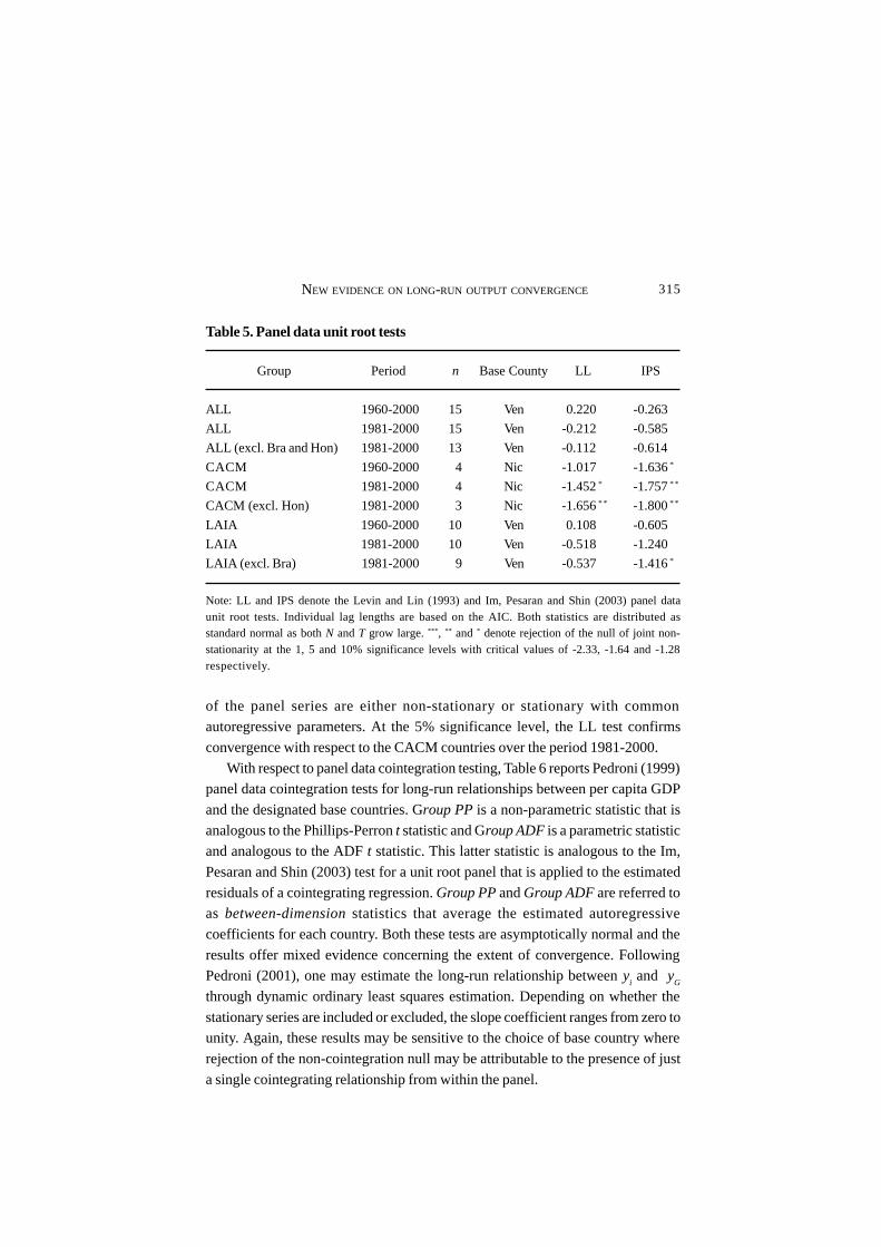
Table 5 reports that the IPS panel data unit root test rejects the null at the 5%significance level in the case of the CACM countries (1981-2000). In all other
cases, the null is accepted at the 5% significance level. These results are consistent
with the results reported in Table 2. However, it should be pointed out that unliketesting the stationarity of the first LPC, the panel data unit root test is sensitive to
the choice of base country and it is possible that acceptance of the null under the
IPS test may simply be due to the choice of base country. Table 5 also reports thefindings from the earlier LL panel data unit root test advocated by Levin and Lin
(1993). This test offers very restrictive joint and null hypotheses where all members
,287.0 1,55 residualslagsLPCconstLPC tt ++−=∆ − (9)
315 NEW EVIDENCE ON LONG-RUN OUTPUT CONVERGENCE
Table 5. Panel data unit root tests
Group Period n Base County LL IPS
ALL 1960-2000 15 Ven 0.220 -0.263
ALL 1981-2000 15 Ven -0.212 -0.585
ALL (excl. Bra and Hon) 1981-2000 13 Ven -0.112 -0.614
CACM 1960-2000 4 Nic -1.017 -1.636*
CACM 1981-2000 4 Nic -1.452* -1.757* *
CACM (excl. Hon) 1981-2000 3 Nic -1.656* * -1.800* *
LAIA 1960-2000 10 Ven 0.108 -0.605
LAIA 1981-2000 10 Ven -0.518 -1.240
LAIA (excl. Bra) 1981-2000 9 Ven -0.537 -1.416*
Note: LL and IPS denote the Levin and Lin (1993) and Im, Pesaran and Shin (2003) panel dataunit root tests. Individual lag lengths are based on the AIC. Both statistics are distributed asstandard normal as both N and T grow large. *** , ** and * denote rejection of the null of joint non-stationarity at the 1, 5 and 10% significance levels with critical values of -2.33, -1.64 and -1.28respectively.
of the panel series are either non-stationary or stationary with commonautoregressive parameters. At the 5% significance level, the LL test confirms
convergence with respect to the CACM countries over the period 1981-2000.
With respect to panel data cointegration testing, Table 6 reports Pedroni (1999)panel data cointegration tests for long-run relationships between per capita GDP
and the designated base countries. Group PP is a non-parametric statistic that is
analogous to the Phillips-Perron t statistic and Group ADF is a parametric statisticand analogous to the ADF t statistic. This latter statistic is analogous to the Im,
Pesaran and Shin (2003) test for a unit root panel that is applied to the estimated
residuals of a cointegrating regression. Group PP and Group ADF are referred toas between-dimension statistics that average the estimated autoregressive
coefficients for each country. Both these tests are asymptotically normal and the
results offer mixed evidence concerning the extent of convergence. FollowingPedroni (2001), one may estimate the long-run relationship between y
i and y
G
through dynamic ordinary least squares estimation. Depending on whether the
stationary series are included or excluded, the slope coefficient ranges from zero tounity. Again, these results may be sensitive to the choice of base country where
rejection of the non-cointegration null may be attributable to the presence of just
a single cointegrating relationship from within the panel.

JOURNAL OF APPLIED ECONOMICS316
Table 6. Panel data cointegration tests
Group Group β tβ=0 tβ=1
PP ADF
ALL 1960-2000 15 Ven 4.853 2.765 N/A N/A N/A
ALL 1981-2000 15 Ven -2.026* * -2.900*** 0.099 -0.323 -7.096***
ALL (excl. Bra
and Hon) 1981-2000 13 Ven -1.837* * -2.024* * 0.481 4.540*** -0.688
CACM 1960-2000 4 Nic 0.684 -0.847 N/A N/A N/A
LAIA 1960-2000 10 Ven 3.869 1.807 N/A N/A N/A
LAIA 1981-2000 10 Ven -0.866 -2.853*** 0.548 1.401 -3.954***
LAIA
(excl. Bra) 1981-2000 9 Ven -0.842 -2.206* * 0.834 3.931*** -0.500
Note: The columns headed Group PP and Group ADF are Pedroni tests for cointegrationbetween y
i and y
G where *** , ** and * denote rejection of the null of joint non-cointegration at
the 1, 5 and 10% significance levels (see Table 5 for critical values). Where the null of non-cointegration is rejected, Column 7 reports the estimated slope (β) and Columns 8 and 9 reportt statistics for the null of a zero and then unity slope. Individual lag lengths are based on theAIC. N/A indicates where the null of non-cointegration is accepted. In these cases, it isinappropriate to report long-run slope estimates and associated t-statistics.
V. Conclusion
This paper has tested for economic convergence among Latin American
countries- a relatively unexplored area- using groupings based on key agreementsconcerning trade liberalization and cooperation. For this purpose, convergence is
addressed in an alternative way through the application of principal components
and cointegration analysis. This multivariate technique has advantages over existingmethods because less demand is placed on limited data sets and the qualitative
outcome of the test is invariant to the choice of base country. In addition to this,
this technique offers a different perspective on convergence based on the co-movements of real per capita outputs rather than the traditional sigma and beta
convergence. There is evidence that convergence is most likely to be found within
convergence clubs based on trade agreements. Using a sample of sixteen LatinAmerican countries, we find that strong long-run convergence is only confirmed
in the cases of the Central American Common Market countries over the period
1960-2000. However, a weaker form of convergence is applicable in the case of theLatin American Integration Association over the period 1981-2000. Such evidence
Group Period n Base

317 NEW EVIDENCE ON LONG-RUN OUTPUT CONVERGENCE
is not present when we consider all Latin American countries considered togetheror groupings that are based on geographical location. The implications of our
findings are twofold. First, it is not necessarily the case that convergence is restricted
to smaller groups of LDCs. For example, we are able to identify the presence of asingle common shared trend driving the eleven countries taken from the Latin
American Integration Association. Second, groupings and sub-periods that exhibit
little or no evidence of convergence provide a case for additional regionaldevelopment policies aimed at facilitating closer integration among member states.
Bearing in mind the findings from this study, several avenues for future research
are brought to light. Researchers may reflect on why some international agreementson increased cooperation are more conducive towards convergence than others.
Future research may also reflect on alternative measures of long-run convergence
perhaps utilizing improved panel data techniques that enable the researcher toidentify which panel members are responsible for rejecting non-stationary or non-
cointegrating null hypotheses.
References
Baldwin, Richard E. (1992), “Measurable dynamic gains from trade”, Journal of
Political Economy 100: 162-74.
Barro, Robert J. (1991), “Economic growth in a cross section of countries”, Quarterly
Journal of Economics 106: 407-43.Barro, Robert J. and Xavier Sala-i-Martin (1991), “Convergence across states and
regions”, Brookings Papers on Economic Activity Issue 1: 107-82.
Barro, Robert J. and Xavier Sala-i-Martin (1992), “Convergence”, Journal of
Political Economy 100: 223-51.
Baumol, William J. (1986), “Productivity, growth, convergence and welfare: What
the long-run data show”, American Economic Review 76: 1072-85.Ben-David, Dan (1993), “Equalizing exchange rate: Trade liberalization and income
convergence”, Quarterly Journal of Economics 108: 653-679.
Ben-David, Dan (1996), “Trade and convergence among countries”, Journal of
International Economics 40: 279-98.
Bernard, Andrew B. and Steven N. Durlauf (1995), “Convergence in international
output”, Journal of Applied Econometrics 10: 97-108.Bernard, Andrew B. and Charles I. Jones (1996), “Comparing apples to oranges:
Productivity convergence and measurement across industries and countries”,
American Economic Review 86: 1216-38.

JOURNAL OF APPLIED ECONOMICS318
Child, Dennis (1970), The Essentials of Factor Analysis, New York, Holt, Reinhart
and Winston.
Choi, Hak and Hongyi Li (2000), “Economic development and growth in China”,
Journal of International Trade and Economic Development 9: 37-54.
Dobson, Stephen and Carlyn Ramlogan (2002), “Economic growth and convergence
in Latin America”, Journal of Development Studies 38: 83-104.
Elliot, Graham, Thomas Rothenberg, and James H. Stock (1996), “Efficient tests for
an autoregressive unit root”, Econometrica 64: 813-36.
Ferreira, Alfonso (2000), “Convergence in Brazil: Recent trends and long-run
prospects”, Applied Economics 32: 79-90.
Findlay, Ronald (1984), “Growth and development in trade models”, in R.W. Jones
and P.B. Kenen, eds., Handbook of International Economics vol. 3, Amsterdam,
Elsevier.
Franses, Philip and Michael McAleer (1998), “Testing for unit roots and non-linear
transformations”, Journal of Time Series Analysis 19: 147-64.
Im, Kyung S., M. Hashem Pesaran, and Yongcheol Shin (2003), “Testing for unit
roots in heterogeneous panels”, Journal of Econometrics 115: 53-74.
Johansen, Soren (1988), “Statistical analysis of cointegrating vectors”, Journal of
Economic Dynamics and Control 12: 231-54.
Khan, Mohsin S. and Manmohan S. Kumar (1993), “Public and private investment
and the convergence of per capita incomes in developing countries”, Working
Paper 93/51, Washington, DC, IMF.
Lane, Philip R. (1997), “International trade and economic convergence”, unpublished
manuscript.
Levin, Andrew, and Chien-Fu Lin (1993), “Unit root tests in panel data: Asymptotic
and finite sample properties”, unpublished manuscript, University of California
at San Diego.
Mankiw, N. Gregory, David Romer, and David N. Weil (1992), “A contribution to
the empirics of economic growth”, Quarterly Journal of Economics 107: 407-
37.
Matsuyama, Kiminori (1996), “Why are there rich and poor countries? Symmetry-
breaking in the world economy”, Journal of the Japanese and International
Economies 10: 419-39.
McCoskey, Suzanne (2002), “Convergence in sub-Saharan Africa: A non-stationary
panel data approach”, Applied Economics 34, 819-29.
Mills, Terry C. and Mark J. Holmes (1999), “Common trends and cycles in European
319 NEW EVIDENCE ON LONG-RUN OUTPUT CONVERGENCE
industrial production: Exchange rate regimes and economic convergence”,
Manchester School 67: 557-87.
Nagaraj, Rayaprolu, Aristomene Varoudakis, and Marie-Ange Veganzones (2000),“Long-run growth trends and convergence across Indian states”, Journal of
International Development 12: 45-70.
Pedroni, Peter (1999), “Critical values for cointegration tests in heterogeneouspanels with multiple regressors”, Oxford Bulletin of Economics and Statistics
61 (special issue): 653-70.
Pedroni, Peter (2001), “Purchasing power parity in cointegrated panels”, Review of
Economics and Statistics 83: 727-731.
Perron, Peter (1997), “Further evidence from breaking trend functions in
macroeconomic variables”, Journal of Econometrics 80: 355-385.Quah, Danny (1996), “Twin peaks: Growth and convergence in models of
distributional dynamics”, Economic Journal 106: 1019-36.
Sachs, Jeffrey and Andrew Warner (1995), “Economic reform and the process ofglobal integration”, Brookings Papers on Economic Activity issue 1: 1-118.
Sala-i-Martin, Xavier (1996), “The classical approach to convergence analysis”,
Economic Journal 106: 1019-36.Slaughter, Matthew, J. (2001), “Trade liberalization and per capita income
convergence: A difference-in-difference analysis”, Journal of International
Economics 55: 203-28.Snell, Andy. (1996), “A test of purchasing power parity based on the largest principal
component of real exchange rates of the main OECD economies”, Economics
Letters 51: 225-31.Stock, James H., and Mark W. Watson (1988), “Testing for common trends”,
Journal of the American Statistical Association 83: 1097-107.
Ventura, Jaume (1997), “Growth and interdependence”, Quarterly Journal of
Economics 112: 57-84.


