
Risk reduction in natural disaster insurance: Experimental
evidence on moral hazard and financial incentives
Jantsje M. Mol
Institute for Environmental Studies (IVM), Vrije Universiteit Amsterdam, The Netherlands
W.J. Wouter Botzen Institute for Environmental Studies (IVM), Vrije Universiteit Amsterdam, The Netherlands
Utrecht University School of Economics, Utrecht University, Utrecht, the Netherlands.
Risk Management and Decision Processes Center, The Wharton School, University of Pennsylvania, USA
E-mail: [email protected]
Julia E. Blasch Institute for Environmental Studies (IVM), Vrije Universiteit Amsterdam, The Netherlands
October 2018
Working Paper # 2018-10
_____________________________________________________________________
Risk Management and Decision Processes Center The Wharton School, University of Pennsylvania
3730 Walnut Street, Jon Huntsman Hall, Suite 500
Philadelphia, PA, 19104, USA Phone: 215-898-5688
Fax: 215-573-2130 https://riskcenter.wharton.upenn.edu/
___________________________________________________________________________

THE WHARTON RISK MANAGEMENT AND DECISION PROCESSES CENTER
Established in 1985, the Wharton Risk Management and Decision Processes Center develops and promotes effective corporate and public policies for low-probability events with potentially catastrophic consequences through the integration of risk assessment, and risk perception with risk management strategies. Natural disasters, technological hazards, and national and international security issues (e.g., terrorism risk insurance markets, protection of critical infrastructure, global security) are among the extreme events that are the focus of the Center’s research.
The Risk Center’s neutrality allows it to undertake large-scale projects in conjunction with other researchers and organizations in the public and private sectors. Building on the disciplines of economics, decision sciences, finance, insurance, marketing and psychology, the Center supports and undertakes field and experimental studies of risk and uncertainty to better understand how individuals and organizations make choices under conditions of risk and uncertainty. Risk Center research also investigates the effectiveness of strategies such as risk communication, information sharing, incentive systems, insurance, regulation and public-private collaborations at a national and international scale. From these findings, the Wharton Risk Center’s research team – over 50 faculty, fellows and doctoral students – is able to design new approaches to enable individuals and organizations to make better decisions regarding risk under various regulatory and market conditions.
The Center is also concerned with training leading decision makers. It actively engages multiple viewpoints, including top-level representatives from industry, government, international organizations, interest groups and academics through its research and policy publications, and through sponsored seminars, roundtables and forums.
More information is available at https://riskcenter.wharton.upenn.edu/.
Risk reduction in natural disaster insurance:
Experimental evidence on moral hazard and financial incentives
Jantsje M. Mol1, W. J. Wouter Botzen1,2,3, and Julia E. Blasch1
October 2018
Abstract
In a world in which economic losses due to natural disasters are expected to increase,
it is important to study risk reduction strategies, including individual investments
of homeowners in damage reducing (mitigation) measures. We use a lab experiment
(N = 357) to investigate the effects of different financial incentives, probability levels
and deductibles on damage reducing investments in a natural disaster insurance market
with compulsory coverage. In particular, we examine how these investments are jointly
influenced by financial incentives, like a disincentive from moral hazard or positive
incentives from premium discounts or a mitigation loan, and behavioral characteristics,
like individual risk and time preferences. We find that investments increase when
the expected value of damage increases (i.e. higher deductibles, higher probabilities).
Moral hazard is found in the high probability scenarios (15%), but not in the low
probability scenarios (3%). This observation suggests that moral hazard is less of an
issue in a natural disaster insurance market where probabilities are low. Our results
demonstrate that a premium discount can increase investments in damage reduction,
as can the behavioral characteristics of risk aversion, perceived efficacy of protective
measures and worry about flooding.
Keywords: Behavioral insurance, Moral hazard, Lab experiment, Natural disasters,
Damage reduction
JEL Codes: B41, C91, C93
1 Institute for Environmental Studies (IVM), Vrije Universiteit Amsterdam, The Netherlands2 Utrecht University School of Economics (USE), Utrecht University, Utrecht, The Netherlands3 Risk Management and Decision Processes Center, The Wharton School, University of Pennsylvania
1 Introduction
Economic losses due to natural disasters, such as floods, have increased in the past 25 years
and it is likely that this trend will continue (IPCC, 2012; Munich RE, 2018). Both the effects
of climate change and ongoing socio-economic development in floodplains contribute to the
projected increase in flood damage (Jongman et al., 2014). This trend leads to a growing
interest in damage reduction strategies, which can be used to manage financial risk (disaster
risk insurance) or reduce the risk altogether (disaster risk reduction). In the case of disaster
risk reduction, most research so far has focused on the role of governments in providing flood
protection infrastructure, such as dikes (Kreibich et al., 2015). Recently, researchers have
started to investigate damage reduction measures that can be taken by private homeowners
and have identified private measures that are cost-effective in reducing flood risk (Poussin
et al., 2015; Kreibich et al., 2011). While the estimated prevented damage can be substantial
(Kreibich et al., 2015), only a small proportion of the homeowners has taken these measures.
The lack of voluntary investment in mitigation measures could be due to the fact that
individuals underestimate disaster risk and the benefits of mitigation measures (Bubeck
et al., 2013; Siegrist and Gutscher, 2008), are risk seeking in the loss domain, heavily discount
future savings in disaster damage, and/or receive insufficient financial incentives for investing
in damage reduction (Kunreuther, 1996, 2015).
Insurance arrangements can be a useful tool to limit the costs of natural disasters by
spreading the risk intertemporally and geographically over a large group of policyholders,
and by providing financial compensation after a disaster which facilitates recovery. Despite
the growing interest in insurance as a tool in disaster risk management, the exact design
of such an insurance arrangement is heavily debated among governments who tend to
focus on affordability and coverage, and the insurance industry who tends to focus on
risk-based pricing and risk reduction (Hudson et al., 2016). In practice, a diversity of
arrangements exists, including private, public and public-private insurance arrangements,
with varying links to risk reduction (Paudel et al., 2012). If insurance arrangements are well
designed they could be combined with financial incentives to invest in damage reduction
measures. However, a potential difficulty in the promotion of damage reduction measures
are information asymmetries between the insurer and the policyholder about implemented
damage reduction measures. These asymmetries can lead to less preventive behavior by
insured individuals since preventive behavior is not factored in their premium if it is not
fully known by the insurer (moral hazard: see Section 2).
To overcome the moral hazard problem, insurance companies have traditionally adopted
deductibles to decrease the coverage of their clients (Winter, 2013). The deductible is the
1

amount of damage that must be paid by the policyholder before the insurer will pay any
expenses, which provides a financial incentive to reduce risk for the policyholder, who now
bears part of the risk him- or herself.
There is little empirical research on the effectiveness of deductibles in the context of
natural disaster risk, except for an econometric analysis of field survey data by Hudson et al.
(2017). They found no positive effect of deductibles on preparation activities for windstorms
in the U.S., except for very high deductible amounts. Other financial incentives can be
provided to stimulate damage reduction investments of homeowners, such as a premium
discount that reflects the reduced damage from policyholder investments in mitigation (Kleindorfer
et al., 2012; Poussin et al., 2014). The purpose of such a premium discount is that it
serves as a financial reward for reducing damage. Finally, low-interest mitigation loans may
be provided by the government or other financial institutions to encourage investment in
damage reduction measures which have high upfront costs, such as flood-proofing a house
(Michel-Kerjan and Kunreuther, 2011). Loans spread the investment costs over time. This
can encourage individuals with high discount rates, i.e. who place a higher weight on more
immediate mitigation costs than future benefits, to invest in damage reduction measures.
So far, no experimental study has investigated a broad range of financial incentives for
damage reduction in an insurance context. Besides, as to our knowledge, moral hazard
has not been studied experimentally in the context of disaster risk, nor in relation to a
variety of probability levels and deductibles. The current study aims to fill this gap by
operationalizing investments in disaster damage reduction in a controlled lab experiment
under different financial incentive treatments, starting from a baseline treatment without
insurance and additional mitigation incentives. This will inform about the (non)existence of
moral hazard in disaster risk contexts. The focus on mandatory insurance closely resembles
the characteristics of many natural disaster insurance markets (Paudel et al., 2012), for which
it is impossible to distill moral hazard by survey and market data, because a control group
without insurance coverage is lacking in practice. Moreover, the causal relationship between
different policy instruments and damage mitigation will be examined, which is another key
advantage of a controlled lab experiment in comparison to survey analysis. The results are
likely to be useful to inform insurance companies and policy makers who aim to increase
both insurance coverage and policyholder damage reduction activities.
The remainder of this article is organized as follows: Section 2 discusses the related
literature, Section 3 describes the experimental design, Section 4 derives hypotheses for each
of the treatments, based on simulations of a theoretical model. Finally, Section 5 presents
results and Section 6 discusses some policy implications and concludes.
2
2 Related literature
This paper relates to three branches of literature which will be discussed next: (1) theoretical
studies of moral hazard in insurance markets; (2) empirical assessments of moral hazard in
actual insurance markets, including natural disaster insurance; and (3) experimental studies
of moral hazard.
Moral hazard was originally formulated by economists as a theoretical concept and a
problem for insurers (Arrow, 1963; Stiglitz, 1974; Arnott and Stiglitz, 1988). Moral hazard
arises when there are information asymmetries between the policyholder and insurer about
damage reduction activities done by the policyholder. In such a case, the policyholder
is not rewarded by damage reduction activities through a lower premium and a moral
hazard effect might arise. This effect implies that insured individuals prepare less for risk
than the uninsured, because the policyholder receives no financial benefit from reducing
risk. The insured expects to receive compensation from the insurer in case of damage,
regardless of risk reduction activities. Depending on the inputs of the model, the extent to
which behavioral motivations and financial incentives have opposing effects, may differ. For
example, expected utility theory predicts that full insurance coverage without deductibles
will crowd out individual risk reduction behavior (Winter, 2013), while high risk aversion
will allow for co-existence of insurance coverage and individual risk reduction investments
(de Meza and Webb, 2001; Hemenway, 1990). de Meza and Webb (2001) showed that in case
of rising premiums, the least risk averse individuals drop out of the market first: this can
result in advantageous selection when the risk averse people remaining in the market, also
take other measures to limit risk. Bajtelsmit and Thistle (2015) modeled the incentives to
gather information about the risks that individuals may impose on others and the interaction
with liability insurance. They found that these incentives may be changed by the availability
of liability insurance and the risk attitude of the potential injurer, where risk averse potential
injurers have incentives to become informed about risk, which makes it more likely they will
limit the risk. Asymmetric information may lead to moral hazard, but under the assumption
of perfect information, socially optimal levels of care will be chosen because the premiums
reflect the investments in care. In sum, whether moral hazard occurs depends on behavioral
characteristics of policyholders, like risk aversion and adjusting premiums to reflect risk
reduction investments may counteract the moral hazard problem and improve preparedness
for risk.
In response to these theoretical predictions, one might turn to empirical data for clarification
of the existence of moral hazard in the context of interest. A large number of studies has
investigated moral hazard empirically in actual insurance markets (see Cohen and Siegelman,
3

2010; Rowell and Connelly, 2012, for an overview), indicating that its existence varies
across markets, depending on the type of insurance product, amongst other factors. Cutler
et al. (2008) examined the relation between insurance take-up, risk levels and risk reducing
activities in five different insurance markets. They found advantageous selection in life
insurance, long-term care insurance and Medigap markets, which they explain by a variation
in risk attitudes in addition to different risk levels. Similarly, Einav et al. (2013) found
a moral hazard effect in the health insurance market by investigating medical spending in
relation to insurance coverage of employees in a large aluminum company in the U.S. Cohen
and Siegelman (2010) argue that empirical work on moral hazard should not aim for a final
conclusion on its fundamental existence, but instead carefully examine the circumstances
under which it will emerge. In this regard, studying natural disaster risks in isolation from
other insurance contexts allows for getting insights into these circumstances in particular
case of natural disasters.
The few survey studies specifically examining natural disaster insurances found that
moral hazard plays only a minor role in voluntary flood insurance markets. Thieken et al.
(2006) surveyed both insurance companies as well as households affected by a flood event
in Germany in 2002. Their analysis shows that approximately one-third of the affected
households did not invest in loss mitigation, but purchased no insurance either. 33.7% of
insured households had no plans to invest in loss mitigation in the future, which compared
to 31.2% of uninsured households, suggests little moral hazard. Petrolia et al. (2015)
focused on wind insurance in coastal areas of the United States. The authors examined
survey data from 790 homeowners with probit and tobit models and found that the same
respondents who buy wind insurance also invest more in wind risk mitigation: the opposite
of moral hazard. Also Osberghaus (2015) analyzed survey data from Germany in 2012 and
found the opposite of moral hazard: households who think they are covered by insurance
have a higher probability to take flood mitigation measures. However, the author warns
against causal inferences from this finding and argues for a correlation interpretation instead.
Hudson et al. (2017) performed an econometric analysis based on data of surveys carried
out in Germany after flood events in 2002, 2005 and 2006, using answers about insurance
take up, flood mitigation measures and subjective risk preferences. They found that flood
insurance purchases were positively related to flood damage reduction behavior of individual
households. In other words: no evidence of moral hazard was found, while advantageous
selection was supported by the data. An advantage of this branch of empirical research is its
high external validity: real market behavior is being used for the analysis. A limitation is that
it is hard to disentangle behavioral characteristics that may explain why individuals both
insure and take risk mitigation measures from the effects of different risk levels and financial
4
incentives. Furthermore, these real market studies focus on voluntary disaster insurance
to create treatment and control groups of insured vs. uninsured individuals. In reality,
many natural disaster insurance systems have mandatory purchase requirements (see e.g.
Den et al., 2017), where the influence of moral hazard and insurance incentives for damage
reduction can only be studied in a lab setting.
A few researchers have examined moral hazard using an experimental approach. The
contexts vary, including the principal-agent paradigm (work effort), field experiments on
default in micro finance and insurance related studies. These experiments show that moral
hazard is less likely to occur (among others) under deterministic losses, low probability of
compensation, joint liability group contracts and available information about government
disaster relief (Berger and Hershey, 1994; Di Mauro, 2002; McKee et al., 2004; Fullbrunn
and Neugebauer, 2013; Bixter and Luhmann, 2014; Biener et al., 2017). We aim to extend the
list of characteristics by systematically studying the effects of different financial incentives,
behavioral characteristics, probability levels and deductibles on damage reduction investments
in the disaster risk insurance context. The focus of this article is on floods, as it is one of
the most costly extreme weather events worldwide with over 26 billion US dollars in losses
in 2017 (Munich RE, 2018). Besides, flood risk insurance is often mandatory or at least
heavily regulated when it is privately insured. These public insurance programs may allow
for a straightforward introduction of integrated financial incentives for risk reduction that
are examined in the lab experiment, in contrast to a private market that is more common
in, for example, storm damage insurance.
3 Experimental design
We examined investment levels in damage reduction under different financial incentives for
mitigation of disaster risk. Participants played 6 independent scenarios of an investment
game under flood risk for multiple rounds. As the experiment was framed in the context of
insurance, all treatments except the No Insurance treatment included a deductible.
The experiment consisted of several individual decision-making tasks, computerized in
oTree (Chen et al., 2016). Earnings were in ECU (Experimental Currency Units) and
converted back to Euros at the end of the game. In the first stage, the initial endowment
was earned, which was invested in a virtual house. As in Laury et al. (2009) participants
were presented with a real effort task to earn this endowment, to overcome the house money
effect (Thaler and Johnson, 1990). Participants were thus confronted with the prospect of
losing instead of winning money (see Harrison and Rutstrom, 2008). A result of an earnings
task where initial earnings are determined by effort could be that it creates variability among
5
subjects, with high performing subjects earning more than low performing subjects, leading
to an unwanted stake effect (Dannenberg et al., 2012). Therefore, a new real effort task was
developed in oTree1, where participants were asked to collect ECU by clicking on a grid of
100 boxes which contained either money or not. The money was randomly distributed by the
software over 60 out of 100 boxes. When 30 boxes with money were collected, the boxes were
deactivated such that all subjects finished with the same budget. To enhance a game-like
situation a timer was placed on the collect money page, though there was no consequence
of collecting fast (nor slow). Screen-shots of the new real effort task can be found on page 2
of the Supplementary Material. After earning their starting capital, participants were asked
to buy a virtual house (worth 240,000 ECU) to be able to play the investment game. The
remainder of the starting capital (75,000 ECU) was stored as ‘savings’ and could be used to
pay for investments, premiums and damages. Subjects were explained that the house was
prone to flood risk.
3.1 Investment game
A scenario started with the introduction of the parameters: flood probability, maximum
damage and deductible level and lasted for 12 rounds. The sequence of pages in each round
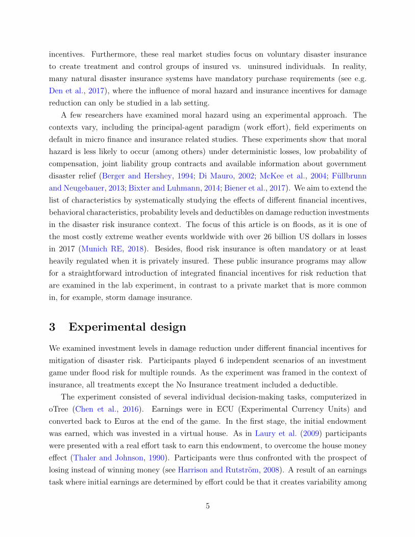
was Invest, Pay premium, Flood risk result. The Invest page offered five discrete investment
levels with accompanying benefits as shown in Figure 1. Investments were effective in damage
reduction for all rounds of a scenario, starting at the round of investment. On the Pay
premium page, subjects paid a fair premium (participants were price-takers). After each
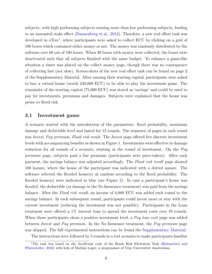
payment, the savings balance was adjusted accordingly. The Flood risk result page showed
100 houses, where the house of the participant was indicated with a dotted square. The
software selected the flooded house(s) at random according to the flood probability. The
flooded house(s) were indicated in blue (see Figure 2). In case a participant’s house was
flooded, the deductible (or damage in the No Insurance treatment) was paid from the savings
balance. After the Flood risk result, an income of 4,000 ECU was added each round to the
savings balance. In each subsequent round, participants could invest more or stay with the
current investment (reducing the investment was not possible). Participants in the Loan
treatment were offered a 1% interest loan to spread the investment costs over 10 rounds.
When those participants chose a positive investment level, a Pay loan cost page was added
between Invest and Pay premium. In the No Insurance treatment, the Pay premium page
was skipped. The full experimental instructions can be found the Supplementary Material.
The instructions were followed by 5 rounds in a test scenario to make participants familiar
1The task was based on the JavaScript code of the Bomb Risk Elicitation Task (Holzmeister andPfurtscheller, 2016) with help of Mathijs Luger, a programmer of Vrije Universiteit Amsterdam.
6
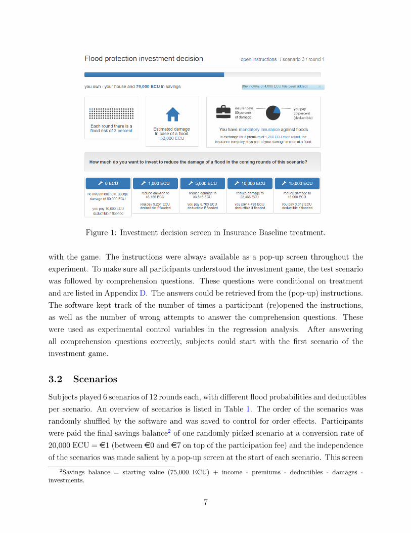
Figure 1: Investment decision screen in Insurance Baseline treatment.
with the game. The instructions were always available as a pop-up screen throughout the
experiment. To make sure all participants understood the investment game, the test scenario
was followed by comprehension questions. These questions were conditional on treatment
and are listed in Appendix D. The answers could be retrieved from the (pop-up) instructions.
The software kept track of the number of times a participant (re)opened the instructions,
as well as the number of wrong attempts to answer the comprehension questions. These
were used as experimental control variables in the regression analysis. After answering
all comprehension questions correctly, subjects could start with the first scenario of the
investment game.
3.2 Scenarios
Subjects played 6 scenarios of 12 rounds each, with different flood probabilities and deductibles
per scenario. An overview of scenarios is listed in Table 1. The order of the scenarios was
randomly shuffled by the software and was saved to control for order effects. Participants
were paid the final savings balance2 of one randomly picked scenario at a conversion rate of
20,000 ECU = e1 (between e0 and e7 on top of the participation fee) and the independence
of the scenarios was made salient by a pop-up screen at the start of each scenario. This screen
2Savings balance = starting value (75,000 ECU) + income - premiums - deductibles - damages -investments.
7
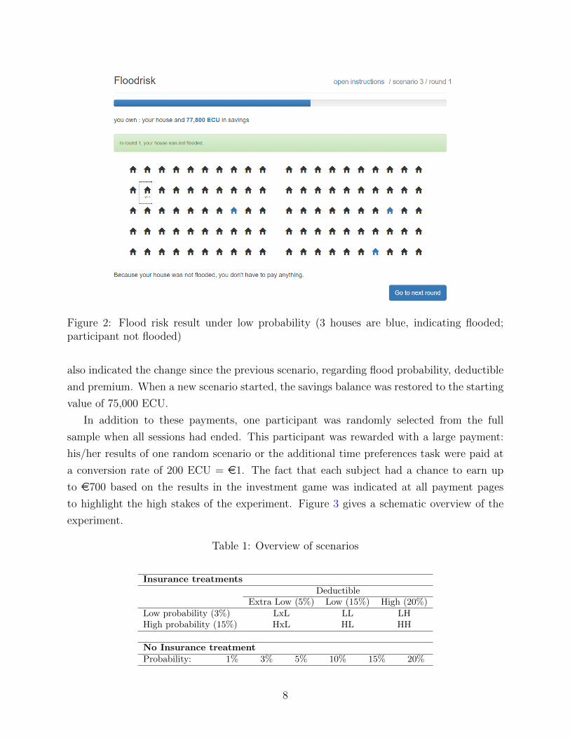
Figure 2: Flood risk result under low probability (3 houses are blue, indicating flooded;participant not flooded)
also indicated the change since the previous scenario, regarding flood probability, deductible
and premium. When a new scenario started, the savings balance was restored to the starting
value of 75,000 ECU.
In addition to these payments, one participant was randomly selected from the full
sample when all sessions had ended. This participant was rewarded with a large payment:
his/her results of one random scenario or the additional time preferences task were paid at
a conversion rate of 200 ECU = e1. The fact that each subject had a chance to earn up
to e700 based on the results in the investment game was indicated at all payment pages
to highlight the high stakes of the experiment. Figure 3 gives a schematic overview of the
experiment.
Table 1: Overview of scenarios
Insurance treatmentsDeductible
Extra Low (5%) Low (15%) High (20%)Low probability (3%) LxL LL LHHigh probability (15%) HxL HL HH
No Insurance treatmentProbability: 1% 3% 5% 10% 15% 20%
8
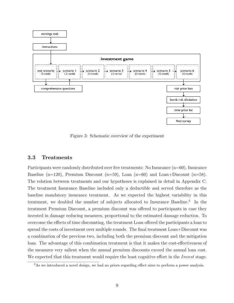
Figure 3: Schematic overview of the experiment
3.3 Treatments
Participants were randomly distributed over five treatments: No Insurance (n=60), Insurance
Baseline (n=120), Premium Discount (n=59), Loan (n=60) and Loan+Discount (n=58).
The relation between treatments and our hypotheses is explained in detail in Appendix C.
The treatment Insurance Baseline included only a deductible and served therefore as the
baseline mandatory insurance treatment. As we expected the highest variability in this
treatment, we doubled the number of subjects allocated to Insurance Baseline.3 In the
treatment Premium Discount, a premium discount was offered to participants in case they
invested in damage reducing measures, proportional to the estimated damage reduction. To
overcome the effects of time discounting, the treatment Loan offered the participants a loan to
spread the costs of investment over multiple rounds. The final treatment Loan+Discount was
a combination of the previous two, including both the premium discount and the mitigation
loan. The advantage of this combination treatment is that it makes the cost-effectiveness of
the measures very salient when the annual premium discounts exceed the annual loan cost.
We expected that this treatment would require the least cognitive effort in the Invest stage.
3As we introduced a novel design, we had no priors regarding effect sizes to perform a power analysis.
9
3.4 Extra tasks
The experiment was followed by a set of questions and decision-tasks to gather data on risk
preferences, time preferences and other behavioral characteristics that could be related to
the investment decisions of the experiment. Risk preferences were measured with two price
lists and the Bomb Risk Elicitation Task (BRET) (Crosetto and Filippin, 2013). Based
on a recent review on risk elicitation tasks (Csermely and Rabas, 2016), we used the new
price list proposed by Drichoutis and Lusk (2016) and did not include the original (Holt
and Laury, 2002) price list. In the new price list, probabilities are held constant at 0.50
and the payoff amounts are varied. This method seems to perform well in forecast accuracy
and it is relatively simple. The same price list was adapted from Drichoutis and Lusk
(2016) and framed in the loss domain. In this task, subjects were first endowed with the
maximum possible loss (e4.70) and the outcomes of the lotteries were negative. In both
price lists, subjects were forced by the oTree software to switch at most once between
options (Holzmeister, 2017): all rows were shown at the screen at once (see screen shots
in Supplementary Material). Finally, a static version of the Bomb Risk Elicitation Task by
Holzmeister and Pfurtscheller (2016) was played once. The BRET contained 100 boxes each
worth e0.05 and one bomb. Subjects were asked to enter a number of boxes, which were
then picked at random and opened by the software. The total value of the opened boxes
was earned by the subject, unless the bomb was among those boxes, which resulted in a
payoff of 0. To prevent income effects, the software selected one of these tasks at random
to be relevant for payment at the end of the three risk elicitation tasks4. The results of
the selected task were shown on the screen and the earnings were saved for payment. For
the time preferences, we used the exact price list of the Preference Module by Falk et al.
(2016) where subjects had to choose 25 times between an immediate payment of e100 and
a delayed payment in 12 months. The delayed payment ranged from e100 to e185. Again,
consistency was enforced by the software (as developed by Holzmeister (2017)). After the
time preferences, one task was selected for the large payment; one of the six scenarios or
the result of the time preferences task. Note that the time preferences task was thus only
incentivized by the large payment; both ‘immediate’ and delayed time preferences payments
would be paid by bank transcription, which resulted in a front end delay with constant
transaction costs. A summary of the payments (participation fee; investment game; risk
elicitation task) was given on the next page. At the end of the experiment, subjects were
asked some socioeconomic questions, qualitative risk and time preferences questions and
some additional questions (e.g. beliefs regarding flood risk). The coding of the questions
4Subjects were informed about this procedure before the start of the first risk elicitation task, whichwere called ‘additional tasks’.
10

can be found in Appendix A.
3.5 Procedure
To test the instructions of the newly developed investment game, a pilot experiment was
carried out in October 2017 with Master students. Subjects were sent a link through which
they could play the game on-line on their own laptop or desktop computer. The pilot
experiment was made available on the server for 1 week. All participants were paid according
to their performance in the game by bank transfer, one week after the pilot. To keep
incentives equal between the pilot and the experiment, all pilot students were eligible for
the large payment. The payment structure was explained verbally in one of their lectures
and again in the invitation e-mail. In total, 20 students took part in the pilot experiment.
On average, they earned approximately e12.00 in 34 minutes. We were mostly interested in
testing the procedure and in the average time to finish the game. The pilot students finished
faster than expected and many of them invested in all scenarios. To increase heterogeneity
in investment decisions across subjects, we added two scenarios to the game with an extra
low deductible and two more risk levels in the No Insurance treatment. To test the length
of the final procedure, a second pilot was conducted among 5 PhD students of our institute.
No major changes were made after the second pilot.
The experiment was conducted in the CREED lab of the University of Amsterdam in
November 2017. A total of 361 participants earned e12.95 on average in 29 minutes. We
conducted 11 sessions in 4 days. Note that subjects were randomly assigned to a treatment
by the software; hence different treatments were played during one experimental session.
Three subjects participated twice due to a minor error with the subject database. The
results of their second experiment have been removed from the analysis. One result was
removed as it was incomplete; this subject did not finish the final survey. This left 357
observations for analysis. All earnings - except the large payment, which included the time
preferences payment - were paid out privately in cash immediately after the experiment. The
large payment was arranged via bank transfer, after all sessions had ended.5
4 Theory and hypotheses
Based on the previous literature in Section 2, we developed several hypotheses that were
tested in the lab experiment. The parameters of the experiment were based on simulations
5Large earnings ranged from e86.70 to e615. The randomly selected participant earned e196.49 fromone of the scenarios. The payment was thus not delayed by 12 months, which could have happened if thetime preferences payment had been selected.
11
of a theoretical model. The following section briefly describes the model, which extends
the expected utility framework on optimal loss mitigation of Kelly and Kleffner (2003) to a
multiple years framework. Note that mitigation refers to investments that reduce the size
of a potential loss but not the probability, which is known as self-insurance in the original
model by Ehrlich and Becker (1972).
4.1 Theoretical framework
First consider the one-year framework. Consider an individual with initial wealth W , who
faces a loss V with probability p and no loss with probability 1 − p. The individual has
the possibility to reduce the size of the loss by implementing mitigation expenditures r.
The effectiveness of mitigation is captured in the mitigation function L(r) that denotes the
maximum possible loss if r is spent on mitigation. If a consumer does not spend anything
on mitigation, the size of the loss will be V . Increasing mitigation expenditures leads to a
decrease of maximum possible loss such that L(0) = V and L′(r) < 0. Finally, assume that
L′′(r) ≤ 0, meaning that the marginal effectiveness of mitigation decreases with an increase
in mitigation expenditures. Insurance coverage is mandatory to protect against the possible
loss, with a coverage of α ∈ [0, 1]. In other words, the insurance contains a deductible of
1 − α per dollar of coverage. The term αL(r) denotes the compensation in case of a loss.
The insurer sets the premium απ, where π = pL(0). The insurer does not observe r and,
hence, does not give premium discounts for risk reduction. The individual will choose a level
of r to maximize expected utility EU :
maxEUr = (1− p)U [W − απ − r] + pU [W − απ − (1− α)L(r)− r] (1)
Now consider the multi-year framework. The model is constructed such that the policyholder
considers a damage reduction investment in the present on the basis of the net present value
of utility in both the present year (in which he considers an investment in mitigation) and
in the years to come. For simplicity, we assume that the policyholder can invest only once,
namely in the first year. A parallel with reality may be that you cannot elevate your house
twice. Thus, the costs of mitigation r are paid in the first year t = 1 only, while the benefits
(a decrease in L) extend in the future up to and including the last year T . Future years are
discounted with a discount factor δ (see Frederick et al., 2002). The individual will choose a
level of r to maximize expected utility EU :
12

maxrEU = (1− p)U [W1 − απ − r] + pU [W1 − απ − (1− α)L(r)− r]
+T∑t=2
1
(1 + δ)t−1
((1− p)U [Wt − απ] + pU [Wt − απ − (1− α)L(r)]
) (2)
4.2 Simulations
We used a comparative statics approach to predict best responses for the simplest hypothesis
(a comparison between Insurance Baseline and No Insurance), reported in Appendix B.
However, no clear-cut analytical solution can be found the other hypotheses. Therefore, we
predicted the best response of risk averse (versus neutral, seeking) and low time discounting
(versus high) individuals investing in mitigation under each treatment based on simulations
of the theory. We used these simulations to set our experimental parameters such that
all hypotheses could be tested with the lab experiment. The results of these simulations,
which are based on Equation 2, are reported in Appendix C. The final set of parameters
includes initial wealth W = 75,000, maximum loss V = 50,000, effectiveness of mitigation
β = 0.00008, number of installments in Loan treatment = 10 and interest rate = 1%. The
following section provides the hypotheses and the intuition behind them.
4.3 Hypotheses
From comparative statics in Appendix B, we know that investments under insurance coverage
(Insurance Baseline) should be lower than in without (No Insurance). In general, Winter
(2013) states that even though moral hazard is considered as a major issue in insurance from
a theoretical perspective, empirical results are mixed. An overview of empirical studies on
moral hazard has been carried out by Cohen and Siegelman (2010). The authors conclude
that the existence of moral hazard is largely dependent on the type of insurance market.
In survey studies moral hazard has been found to play only a minor role in voluntary flood
insurance markets (Hudson et al., 2017; Thieken et al., 2006). Therefore, the first hypothesis
concerns the role of moral hazard in the flood risk insurance context. Under simulations of
the theory, damage reduction investments in the Insurance Baseline treatment are lower than
in the No Insurance treatment. Positive investments in the Insurance Baseline treatment
may be optimal in high probability scenarios, depending on the deductible level and attitude
to risk.
Hypothesis 1 Damage reduction investments in the Insurance Baseline treatment are lower
than in the No Insurance treatment, but greater than zero.
13

Hudson et al. (2017) argue that in natural disaster markets, decisions are mainly driven
by risk attitudes, where highly risk averse individuals take several precautionary measures
available, including both flood insurance and flood damage reduction measures. In this
scenario, advantageous selection may prevail over the moral hazard effect, which may be
explained by a misunderstanding of risk (Kunreuther and Pauly, 2004). However, Hudson
et al. (2017) did not examine the behavioral mechanisms to back up their claim. The current
experiment aims to fill that gap. The simulations show that risk-seeking individuals should
not invest in the Insurance Baseline and Loan treatments, while investing 1,000 or 5,000 could
be optimal for risk-neutral individuals and investing 10,000 could be optimal for risk-averse
individuals.
Hypothesis 2 Risk-averse individuals will invest more in damage reduction in the Insurance
Baseline treatment and the Loan treatment than risk-neutral individuals, where risk-seeking
individuals will invest less.
In line with risk based insurance premiums, researchers (Kunreuther, 1996; Surminski
et al., 2015) as well as policymakers (European Commission, 2013) have suggested that a
premium discount may motivate policyholders to take mitigation measures. So far there
is little empirical evidence on the effectiveness of premium discounts, except for Botzen
et al. (2009), who surveyed a large sample of Dutch homeowners in floodplains about their
willingness to pay for low cost flood mitigation measures. They found that the main incentive
for investment was the premium discount on the flood insurance policy that was offered in
the survey (Botzen et al., 2009). The third hypothesis concerns the Premium Discount
treatment. The simulations show that damage reduction investments should be higher in
the Premium Discount treatment compared to the Insurance Baseline treatment under all
scenarios and risk attitudes.
Hypothesis 3 Damage reduction investments are higher in the Premium Discount treatment
than in the Insurance Baseline treatment.
A second financial incentive to promote policyholder damage reduction measures is a
mitigation loan, or a payment in installments (Michel-Kerjan, 2010), aimed at individuals
who heavily discount the future. Even though policyholder damage reduction measures may
be cost-effective under expected utility theory (Kreibich et al., 2015), these short-sighted or
myopic individuals weigh the present costs much heavier than projected future benefits. A
mitigation loan may convince those individuals by spreading the costs over multiple periods.
Damage reduction investments are lower in the Insurance Baseline and Premium Discount
treatments under high time discounting, according to our simulations. In the Loan and
Loan+Discount treatments, time discounting has no effect on damage reduction investments.
14

Hypothesis 4 Damage reduction investments are lower for participants with high time
discount rates. This effect is strongest in the Insurance Baseline and Premium Discount
treatments, but disappears in the Loan and Loan+Discount treatments.
A combination of the Loan and the Discount treatment requires the least cognitive
effort to identify attractive investments. Furthermore, this treatment could overcome both
high time discounting and a moral hazard effect. The Loan+Discount treatment could
be powerful assuming that a considerate share of individuals is risk averse and present
oriented. Therefore, we expect that the combination of incentives leads to the highest
damage reduction investments. The simulations support that Loan+Discount gives the
highest optimal investments of all treatments in the low probability scenarios.
Hypothesis 5 Damage reduction investments are highest in the Loan+Discount treatment.
15
5 Results
This section reports our results, starting with a trend analysis of investments over the 12
rounds of the investment game. Subsequently, we present a non-parametric analysis of the
between-subject treatments and we analyze individual determinants of investment behavior
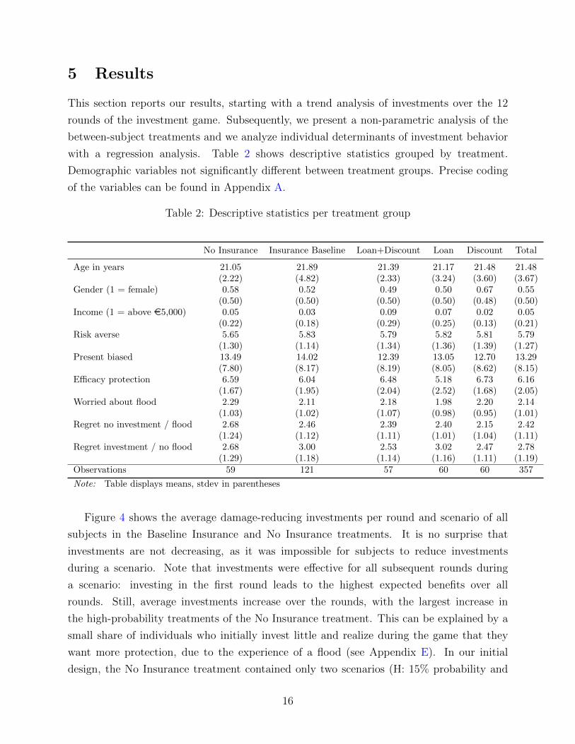
with a regression analysis. Table 2 shows descriptive statistics grouped by treatment.
Demographic variables not significantly different between treatment groups. Precise coding
of the variables can be found in Appendix A.
Table 2: Descriptive statistics per treatment group
No Insurance Insurance Baseline Loan+Discount Loan Discount Total
Age in years 21.05 21.89 21.39 21.17 21.48 21.48(2.22) (4.82) (2.33) (3.24) (3.60) (3.67)
Gender (1 = female) 0.58 0.52 0.49 0.50 0.67 0.55(0.50) (0.50) (0.50) (0.50) (0.48) (0.50)
Income (1 = above e5,000) 0.05 0.03 0.09 0.07 0.02 0.05(0.22) (0.18) (0.29) (0.25) (0.13) (0.21)
Risk averse 5.65 5.83 5.79 5.82 5.81 5.79(1.30) (1.14) (1.34) (1.36) (1.39) (1.27)
Present biased 13.49 14.02 12.39 13.05 12.70 13.29(7.80) (8.17) (8.19) (8.05) (8.62) (8.15)
Efficacy protection 6.59 6.04 6.48 5.18 6.73 6.16(1.67) (1.95) (2.04) (2.52) (1.68) (2.05)
Worried about flood 2.29 2.11 2.18 1.98 2.20 2.14(1.03) (1.02) (1.07) (0.98) (0.95) (1.01)
Regret no investment / flood 2.68 2.46 2.39 2.40 2.15 2.42(1.24) (1.12) (1.11) (1.01) (1.04) (1.11)
Regret investment / no flood 2.68 3.00 2.53 3.02 2.47 2.78(1.29) (1.18) (1.14) (1.16) (1.11) (1.19)
Observations 59 121 57 60 60 357
Note: Table displays means, stdev in parentheses
Figure 4 shows the average damage-reducing investments per round and scenario of all
subjects in the Baseline Insurance and No Insurance treatments. It is no surprise that
investments are not decreasing, as it was impossible for subjects to reduce investments
during a scenario. Note that investments were effective for all subsequent rounds during
a scenario: investing in the first round leads to the highest expected benefits over all
rounds. Still, average investments increase over the rounds, with the largest increase in
the high-probability treatments of the No Insurance treatment. This can be explained by a
small share of individuals who initially invest little and realize during the game that they
want more protection, due to the experience of a flood (see Appendix E). In our initial
design, the No Insurance treatment contained only two scenarios (H: 15% probability and
16

L: 3% probability), where all other treatments tested 6 different scenarios. To keep the
workload for all participants approximately equal, we added 4 scenarios to the No Insurance
treatment to study the effect of expected value of flood losses on investments with a more
refined pattern of probabilities. Figure 4 also shows that subjects indeed invested more when
the expected value of a loss increased (i.e. higher deductible and/or higher probability).
These extra probability scenarios in the No Insurance treatment are not included in any
further analyses.
Figure 4: Average investment in damage reducing measures by scenario
The main analysis presented here will focus on the first round only for the non-parametric
analysis and all panel data is used for the regression analysis. To answer Hypothesis 1
we compared the investment levels in the first round between Insurance Baseline (with
the medium deductible level of 15%) and No Insurance treatments. Figure 5 depicts the
results. A one-sided t-test revealed that the average investment in the first round of Insurance
Baseline was significantly higher than 0 both in the high-probability scenario (MBaselineHL =
4049.59, t = 9.20, df = 120, p < 0.0000) and in the low-probability scenario (MBaselineLL =
2404.96, t = 6.22, df = 120, p < 0.0000). Wilcoxon rank-sum tests showed that the
investments in No Insurance are significantly higher than in Insurance Baseline for the high
probability scenarios
(MNoInsuranceH = 7288.14, z = 3.616, p = 0.0003) but not for the low probability scenarios
(MNoInsuranceL = 2711.86, z = 0.856, p = 0.3918). These findings provide evidence for
Hypothesis 1.
The fact that there is no significant difference between investments in the No Insurance
and Insurance Baseline treatments in the low probability scenario, suggests that there is no
17
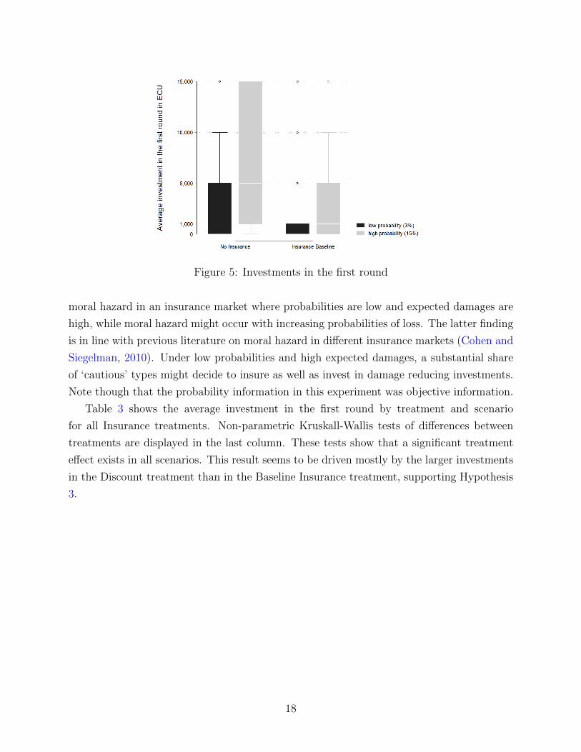
Figure 5: Investments in the first round
moral hazard in an insurance market where probabilities are low and expected damages are
high, while moral hazard might occur with increasing probabilities of loss. The latter finding
is in line with previous literature on moral hazard in different insurance markets (Cohen and
Siegelman, 2010). Under low probabilities and high expected damages, a substantial share
of ‘cautious’ types might decide to insure as well as invest in damage reducing investments.
Note though that the probability information in this experiment was objective information.
Table 3 shows the average investment in the first round by treatment and scenario
for all Insurance treatments. Non-parametric Kruskall-Wallis tests of differences between
treatments are displayed in the last column. These tests show that a significant treatment
effect exists in all scenarios. This result seems to be driven mostly by the larger investments
in the Discount treatment than in the Baseline Insurance treatment, supporting Hypothesis
3.
18
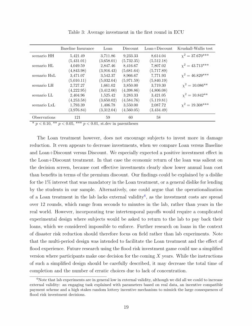
Table 3: Average investment in the first round in ECU
Baseline Insurance Loan Discount Loan+Discount Kruskall-Wallis test
scenario HH 5,421.49 3,711.86 9,233.33 8,614.04 χ2 = 37.670***(5,431.01) (3,658.01) (5,732.35) (5,512.18)
scenario HL 4,049.59 2,847.46 8,416.67 7,807.02 χ2 = 43.713***(4,843.98) (3,916.43) (5,681.64) (5,717.89)
scenario HxL 3,471.07 3,542.37 8,966.67 7,771.93 χ2 = 46.829***(5,010.11) (5,032.04) (5,971.59) (5,840.19)
scenario LH 2,727.27 1,661.02 3,850.00 3,719.30 χ2 = 10.086**(4,222.95) (3,412.00) (4,398.86) (4,806.08)
scenario LL 2,404.96 1,525.42 3,283.33 3,421.05 χ2 = 10.842**(4,253.58) (3,650.02) (4,584.76) (5,119.81)
scenario LxL 1,793.39 1,406.78 3,550.00 2,087.72 χ2 = 19.308***(3,976.84) (3,312.04) (4,560.05) (3,434.49)
Observations 121 59 60 58
* p < 0.10, ** p < 0.05, *** p < 0.01, st.dev in parentheses
The Loan treatment however, does not encourage subjects to invest more in damage
reduction. It even appears to decrease investments, when we compare Loan versus Baseline
and Loan+Discount versus Discount. We especially expected a positive investment effect in
the Loan+Discount treatment. In that case the economic return of the loan was salient on
the decision screen, because cost effective investments clearly show lower annual loan cost
than benefits in terms of the premium discount. Our findings could be explained by a dislike
for the 1% interest that was mandatory in the Loan treatment, or a general dislike for lending
by the students in our sample. Alternatively, one could argue that the operationalization
of a Loan treatment in the lab lacks external validity6, as the investment costs are spread
over 12 rounds, which range from seconds to minutes in the lab, rather than years in the
real world. However, incorporating true intertemporal payoffs would require a complicated
experimental design where subjects would be asked to return to the lab to pay back their
loans, which we considered impossible to enforce. Further research on loans in the context
of disaster risk reduction should therefore focus on field rather than lab experiments. Note
that the multi-period design was intended to facilitate the Loan treatment and the effect of
flood experience. Future research using the flood risk investment game could use a simplified
version where participants make one decision for the coming X years. While the instructions
of such a simplified design should be carefully described, it may decrease the total time of
completion and the number of erratic choices due to lack of concentration.
6Note that lab experiments are in general low in external validity, although we did all we could to increaseexternal validity: an engaging task explained with parameters based on real data, an incentive compatiblepayment scheme and a high stakes random lottery incentive mechanism to mimick the large consequences offlood risk investment decisions.
19
In addition to the non-parametric analysis, we examined the individual determinants of
investment behavior with a regression analysis. All explanatory variables were checked for
high correlations to rule out issues of multicollinearity. As all correlation coefficients were
smaller than 0.5, multicollinearity was not regarded as problematic (Field, 2009).
Table 4 shows random-effects panel regression ML estimates with treatment dummies.
The dependent variable is the log-transformed7 damage reducing investment. The model
has a panel specification to account for the correlation of decisions by the same subject. We
clustered standard errors by id (subject) and scenario. All models control for (1) attempts
to answer understanding questions8, (2) perceived difficulty, (3) flood risk perception, (4)
one over round to control for experience, (5) order of scenario and (6) order of scenario ×probability interaction, but coefficients have been suppressed for brevity. Damage reducing
investments declined when a scenario appeared later in the experiment. Model 1 considers
only treatment and scenario dummies. The positive coefficients of the Discount treatment
confirm the results of the non-parametric analysis: a premium discount leads to higher
investments, as predicted by Hypothesis 3. This effect is large and statistically significant
under all possible controls. The negative effect of the mitigation loan on investments
from the non-parametric analysis is not confirmed for all models and the estimates are not
significant. The combination of Loan and Discount has positive but insignificant estimates.
Discount alone leads to the highest investments, and because there is no additional increase
in investments from loans, Hypothesis 5 finds no support in the data. Another robust
finding is that subjects invest more when the expected damage of a flood rises (higher
probability and higher deductible level). Model 2 includes three control variables that varied
over rounds: participant flooded in the previous round, direct neighbors (see Figure 6)
flooded in the previous round and decision time in seconds at the Invest screen. The positive
and significant estimate for decision time shows that investments are higher when subjects
spend more time on the Invest page. This effect may be explained by the decisions in the first
round that require some deliberation, while subjects learn to move quickly to the next page
without extra investments in later rounds. The neighbor variable was constructed to control
for erroneous feelings of spatial correlations between floods in the game. Both participant
and neighbor flooded variables are not significant. Note that the dependent variable here
is log-transformed investment, which may not differ a lot over rounds. In Appendix E we
analyze ‘extra investments’ specifically and there we do find that subjects invest extra in
damage reduction after experiencing a flood in the game, but not when a neighbor has been
7We used the transformation transformed = log(investment+ 1) to deal with 0 investments.8One subject attempted the comprehension questions more than 10 times. For robustness, we re-ran all
analyses excluding this subject. The results do not change qualitatively.
20

flooded.
Figure 6: Grey color indicates direct neighbors for construction of neighbors variable
Model 3 includes demographic variables. All else equal, we find that investments decrease
slightly with age, that women invest significantly more than men and that subjects with
a high income in real life invest less in damage reduction in the game. The risk averse
variable is a linear combination of our four risk elicitation methods9, as in Menkhoff and
Sakha (2017). Risk averse subjects invest more in damage reducing investments, providing
evidence for Hypothesis 2. Table E.1 provides additional robustness checks for each of the
four risk elicitation methods separately. The direction of the risk aversion effect is equal for
all elicitation methods and the estimates of other variables do not change qualitatively. We
find no effect of time discounting on investments10, suggesting no support for Hypothesis
4. However, the operationalization of the Loan treatment may not have been optimal to
mimic a long investment term, as the investment costs were spread over 12 rounds, which
passed by in minutes, rather than years. In Model 4 we further include variables concerning
flood beliefs. We find a significant and positive coefficient of believed efficacy of protective
measures and worry about flooding. A significant negative estimate is found for regret of
investment. Note that this question was asked after the experiment had ended. The causal
direction is thus likely to be reversed: subjects who invested significantly less indicated in
the post-experimental survey that they felt regret about investing when no flood occurred.
9See Section 3.4 for a description of these tasks.10We have included an interaction term of time discounting × Loan, but the results were not statistically
significant.
21
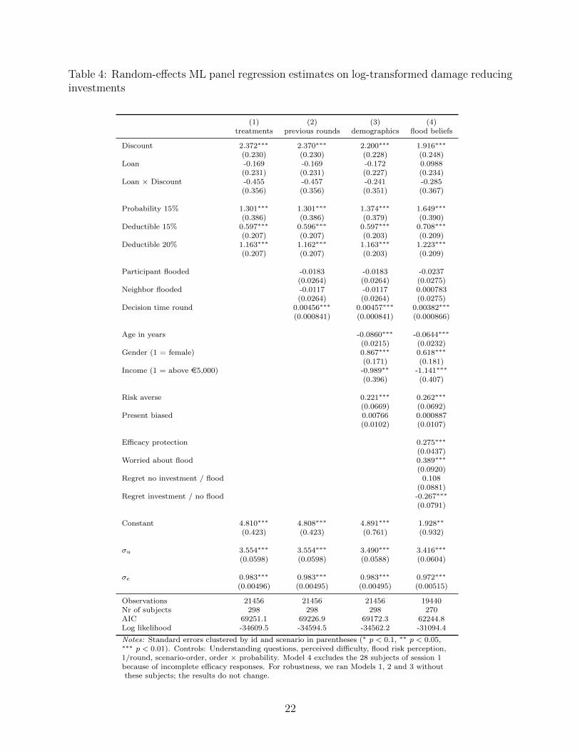
Table 4: Random-effects ML panel regression estimates on log-transformed damage reducinginvestments
(1) (2) (3) (4)treatments previous rounds demographics flood beliefs
Discount 2.372∗∗∗ 2.370∗∗∗ 2.200∗∗∗ 1.916∗∗∗
(0.230) (0.230) (0.228) (0.248)Loan -0.169 -0.169 -0.172 0.0988
(0.231) (0.231) (0.227) (0.234)Loan × Discount -0.455 -0.457 -0.241 -0.285
(0.356) (0.356) (0.351) (0.367)
Probability 15% 1.301∗∗∗ 1.301∗∗∗ 1.374∗∗∗ 1.649∗∗∗
(0.386) (0.386) (0.379) (0.390)Deductible 15% 0.597∗∗∗ 0.596∗∗∗ 0.597∗∗∗ 0.708∗∗∗
(0.207) (0.207) (0.203) (0.209)Deductible 20% 1.163∗∗∗ 1.162∗∗∗ 1.163∗∗∗ 1.223∗∗∗
(0.207) (0.207) (0.203) (0.209)
Participant flooded -0.0183 -0.0183 -0.0237(0.0264) (0.0264) (0.0275)
Neighbor flooded -0.0117 -0.0117 0.000783(0.0264) (0.0264) (0.0275)
Decision time round 0.00456∗∗∗ 0.00457∗∗∗ 0.00382∗∗∗
(0.000841) (0.000841) (0.000866)
Age in years -0.0860∗∗∗ -0.0644∗∗∗
(0.0215) (0.0232)Gender (1 = female) 0.867∗∗∗ 0.618∗∗∗
(0.171) (0.181)Income (1 = above e5,000) -0.989∗∗ -1.141∗∗∗
(0.396) (0.407)
Risk averse 0.221∗∗∗ 0.262∗∗∗
(0.0669) (0.0692)Present biased 0.00766 0.000887
(0.0102) (0.0107)
Efficacy protection 0.275∗∗∗
(0.0437)Worried about flood 0.389∗∗∗
(0.0920)Regret no investment / flood 0.108
(0.0881)Regret investment / no flood -0.267∗∗∗
(0.0791)
Constant 4.810∗∗∗ 4.808∗∗∗ 4.891∗∗∗ 1.928∗∗
(0.423) (0.423) (0.761) (0.932)
σu 3.554∗∗∗ 3.554∗∗∗ 3.490∗∗∗ 3.416∗∗∗
(0.0598) (0.0598) (0.0588) (0.0604)
σe 0.983∗∗∗ 0.983∗∗∗ 0.983∗∗∗ 0.972∗∗∗
(0.00496) (0.00495) (0.00495) (0.00515)
Observations 21456 21456 21456 19440Nr of subjects 298 298 298 270AIC 69251.1 69226.9 69172.3 62244.8Log likelihood -34609.5 -34594.5 -34562.2 -31094.4
Notes: Standard errors clustered by id and scenario in parentheses (∗ p < 0.1, ∗∗ p < 0.05,∗∗∗ p < 0.01). Controls: Understanding questions, perceived difficulty, flood risk perception,1/round, scenario-order, order × probability. Model 4 excludes the 28 subjects of session 1because of incomplete efficacy responses. For robustness, we ran Models 1, 2 and 3 withoutthese subjects; the results do not change.
22

6 Conclusion
Given the increase of economic losses due to natural disasters, interest in damage reduction
strategies has been growing. A recent branch of this research focuses on cost-effective
measures that can be taken by private homeowners. This study contributed to the field by
investigating a broad range of financial incentives for damage reduction in the context of flood
insurance by means of a controlled lab experiment (N = 357). A new investment game under
flood risk was developed to study the causal relationship between policy instruments and
damage reducing investments, taking into account behavioral characteristics of individuals
in a flood insurance market with mandatory coverage. We found that subjects invested more
when the expected value of a loss increased (higher deductible and/or higher probability of
flood). As hypothesized, we identified that the investments in the No Insurance treatment
were significantly higher than in the Insurance Baseline treatment for the high probability
(15%) scenarios, but not significantly different in the low (3%) probability scenarios. Mean
investments in Insurance Baseline were larger than zero, confirming our conjecture that
moral hazard is less of a problem in a natural disaster insurance market where probabilities
of loss are small and expected damages are high. Experiencing a flood in the game triggers
extra investments in flood damage mitigation measures. It is more beneficial if people take
such measures before, instead of after, a flood, which highlights the need to explore the
effectiveness of incentives that motivate people to reduce risk ex ante flood events.
Regarding financial incentives for damage reduction, our results demonstrate that a
premium discount can increase investments in damage reduction. Behavioral characteristics
that have a positive effect on these investments are risk aversion, perceived efficacy of
protective measures and worry about flooding. Implications of our findings are that the
policyholders should be well informed about cost-effective ways to reduce damage, and that
appeals to negative feelings toward flooding (in terms of worry) may stimulate people to
invest more in flood damage mitigation measures. Although deductibles have a significant
influence on damage reduction, the size of this effect is not very large which questions the
usefulness of using high deductibles to stimulate policyholder flood risk reduction activities.
Moreover, our finding that moral hazard effects of insurance are minor suggests that there
is less of a need for high deductibles to limit such an effect. Using premiums discounts is
likely to be a more effective way for insurers to stimulate policyholders to reduce flood risk.
Future work could examine the behavior of homeowners in floodplains, who might respond
differently as they have more experience with insurance and possibly flooding than the
current student sample. The interplay of financial incentives and behavioral characteristics
in voluntary disaster insurance schemes is another important topic for future research.
23

References
Aerts, J. C. J. H., Botzen, W. J. W., de Moel, H., and Bowman, M. (2013). Cost estimates for floodresilience and protection strategies in New York City. Annals of the New York Academy of Sciences,1294(1):1–104.
Arnott, R. J. and Stiglitz, J. E. (1988). The basic analytics of moral hazard. Scandinavian Journal ofEconomics, 90(3):383–413.
Arrow, K. J. (1963). Uncertainty and the welfare economics of medical care. American Economic Review,53(5):141–149.
Bajtelsmit, V. and Thistle, P. (2015). Liability, Insurance and the Incentive to Obtain Information aboutRisk. The Geneva Risk and Insurance Review, 40(2):171–193.
Berger, L. A. and Hershey, J. C. (1994). Moral hazard, risk seeking, and free riding. Journal of Risk andUncertainty, 9(2):173–186.
Biener, C., Eling, M., Landmann, A., and Pradhan, S. (2017). Can group incentives alleviate moralhazard? the role of pro-social preferences. European Economic Review, pages 1–18.
Bixter, M. T. and Luhmann, C. C. (2014). Shared losses reduce sensitivity to risk: A laboratory study ofmoral hazard. Journal of Economic Psychology, 42(December):63–73.
Botzen, W. J. W., Aerts, J. C. J. H., and van den Bergh, J. C. J. M. (2009). Willingness of homeowners tomitigate climate risk through insurance. Ecological Economics, 68(8-9):2265–2277.
Bubeck, P., Botzen, W. J. W., Kreibich, H., and Aerts, J. C. J. H. (2013). Detailed insights into theinfluence of flood-coping appraisals on mitigation behaviour. Global Environmental Change,23(5):1327–1338.
Chen, D. L., Schonger, M., and Wickens, C. (2016). oTree - An open-source platform for laboratory, online,and field experiments. Journal of Behavioral and Experimental Finance, 9:88–97.
Cohen, A. and Siegelman, P. (2010). Testing for adverse selection in insurance markets. Journal of Riskand Insurance, 77(1):39–84.
Crosetto, P. and Filippin, A. (2013). The bomb risk elicitation task. Journal of Risk and Uncertainty,47:31–65.
Csermely, T. and Rabas, A. (2016). How to reveal peoples preferences: Comparing time consistency andpredictive power of multiple price list risk elicitation methods. Journal of Risk and Uncertainty,53(2-3):107–136.
Cutler, D. M., Finkelstein, A., and McGarry, K. (2008). Preference heterogeneity and insurance markets:Explaining a puzzle of insurance. The American Economic Review, 98(2):157–162.
Dannenberg, A., Riechmann, T., Sturm, B., and Vogt, C. (2012). Inequality aversion and the house moneyeffect. Experimental Economics, 15(3):460–484.
de Meza, D. and Webb, D. C. (2001). Advantageous selection in insurance markets. RAND Journal ofEconomics, 32(2):249–262.
Den, X. L., Persson, M., Benoist, A., Hudson, P., Ruiter, M. C. d., and Ruig, L. d. (2017). Insurance ofweather and climate- related disaster risk: Inventory and analysis of mechanisms to support damageprevention in the EU. Technical Report August, European Commission, Brussels.
Di Mauro, C. (2002). Ex ante an ex post moral hazard in compensation for income losses: results from anexperiment. Journal of Socio-Economics, 31(3):253–271.
Drichoutis, A. C. and Lusk, J. L. (2016). What can multiple price lists really tell us about risk preferences?Journal of Risk and Uncertainty, 53(2-3):89–106.
Ehrlich, I. and Becker, G. S. (1972). Market insurance, self-insurance and self-protection. Journal ofPolitical Economy, 80(4):623–648.
Einav, L., Finkelstein, A., Ryan, S. P., Schrimpf, P., and Cullen, M. R. (2013). Selection on moral hazardin health insurance. The American Economic Review, 103(1):178–219.
European Commission, . (2013). Green Paper on the insurance of natural and man-made disasters.Technical report, European Commission, Strasbourg.
Falk, A., Becker, A., Dohmen, T., Huffman, D., and Sunde, U. (2016). The preference survey module: Avalidated instrument for measuring risk, time, and social preferences.
Field, A. (2009). Discovering statistics using SPSS. SAGE Publications, London, 3rd edition.Frederick, S., Loewenstein, G., and O’Donoghue, T. (2002). Time discounting and time preference: A
24
critical review. Journal of Economic Literature, 40(2):351–401.Fullbrunn, S. and Neugebauer, T. (2013). Limited liability, moral hazard, and risk taking: A safety net
game experiment. Economic Inquiry, 51(2):1389–1403.Harrison, G. W. and Rutstrom, E. E. (2008). Risk aversion in the laboratory. In Research in Experimental
Economics, volume 12, pages 41–196. Emeral Group Publishing Limited.Hemenway, D. (1990). Propitious selection. The Quarterly Journal of Economics, 105(4):1063–1069.Holt, C. A. and Laury, S. K. (2002). Risk aversion and incentive effects. American Economic Review,
92(5):1644–1655.Holzmeister, F. (2017). oTree: Ready-made apps for risk preference elicitation methods. Journal of
Behavioral and Experimental Finance.Holzmeister, F. and Pfurtscheller, A. (2016). oTree: The bomb risk elicitation task. Journal of Behavioral
and Experimental Finance, 10:105–108.Hudson, P., Botzen, W. J. W., Czajkowski, J., and Kreibich, H. (2017). Moral hazard in natural disaster
insurance markets: Empirical evidence from Germany and the United States. Land Economics,93(2):179–208.
Hudson, P., Botzen, W. J. W., Feyen, L., and Aerts, J. C. J. H. (2016). Incentivising flood risk adaptationthrough risk based insurance premiums: Trade-offs between affordability and risk reduction. EcologicalEconomics, 125(November):1–13.
IPCC (2012). Managing the risks of extreme events and disasters to advance climate change adaptation.Cambridge University Press.
Jongman, B., Hochrainer-Stigler, S., Feyen, L., Aerts, J. C. J. H., Mechler, R., Botzen, W. J. W., Bouwer,L. M., Pflug, G., Rojas, R., and Ward, P. J. (2014). Increasing stress on disaster-risk finance due tolarge floods. Nature Climate Change, 4(4):1–5.
Kelly, M. and Kleffner, A. E. (2003). Optimal loss mitigation and contract design. The Journal of Risk andInsurance, 70(1):53–72.
Kleindorfer, P. R., Kunreuther, H. C., and Ou-Yang, C. (2012). Single-year and multi-year insurancepolicies in a competitive market. Journal of Risk and Uncertainty, 45(1):51–78.
Kreibich, H., Bubeck, P., van Vliet, M., and De Moel, H. (2015). A review of damage-reducing measures tomanage fluvial flood risks in a changing climate. Mitigation and Adaptation Strategies for GlobalChange, 20(6):967–989.
Kreibich, H., Christenberger, S., and Schwarze, R. (2011). Economic motivation of households to undertakeprivate precautionary measures against floods. Natural Hazards and Earth System Science,11(2):309–321.
Kunreuther, H. C. (1996). Mitigating disaster losses through insurance. Journal of Risk and Uncertainty,12:171–187.
Kunreuther, H. C. (2015). The role of insurance in reducing losses from extreme events: The need forpublic-private partnerships. Geneva Papers on Risk and Insurance: Issues and Practice, 40(4):741–762.
Kunreuther, H. C. and Pauly, M. V. (2004). Neglecting disaster: Why don’t people insure against largelosses? Journal of Risk and Uncertainty, 28(1):5–21.
Laury, S. K., McInnes, M. M., and Todd Swarthout, J. (2009). Insurance decisions for low-probabilitylosses. Journal of Risk and Uncertainty, 39(1):17–44.
McKee, M., Berrens, R. P., Jones, M. L., Helton, R., and Talberth, J. (2004). Using experimentaleconomics to examine wildfire insurance and averting decisions in the WildlandUrban Interface. Society& Natural Resources, 17(6):491–507.
Menkhoff, L. and Sakha, S. (2017). Estimating risky behavior with multiple-item risk measures. Journal ofEconomic Psychology, 59:59–86.
Michel-Kerjan, E. O. (2010). Catastrophe economies: The National Flood Insurance Program. TheJournal of Economic Perspectives, 24(4):165–186.
Michel-Kerjan, E. O. and Kunreuther, H. C. (2011). Redesigning flood insurance. Science, 333:408–409.Munich RE, . (2018). Natural catastrophe review: Series of hurricanes makes 2017 year of highest insured
losses ever.Osberghaus, D. (2015). The determinants of private flood mitigation measures in Germany - Evidence
from a nationwide survey. Ecological Economics, 110:36–50.Paudel, Y., Botzen, W. J. W., and Aerts, J. C. J. H. (2012). A comparative study of publicprivate
25

catastrophe insurance systems: Lessons from current practices. The Geneva Papers on Risk andInsurance Issues and Practice, 37(2):603–603.
Petrolia, D. R., Hwang, J., Landry, C. E., and Coble, K. H. (2015). Wind insurance and mitigation in thecoastal zone. Land Economics, 91(2):272–295.
Poussin, J. K., Botzen, W. J. W., and Aerts, J. C. J. H. (2014). Factors of influence on flood damagemitigation behaviour by households. Environmental Science and Policy, 40:69–77.
Poussin, J. K., Wouter Botzen, W. J., and Aerts, J. C. J. H. (2015). Effectiveness of flood damagemitigation measures: Empirical evidence from French flood disasters. Global Environmental Change,31:74–84.
Rowell, D. and Connelly, L. B. (2012). A history of the term ”moral hazard”. Journal of Risk andInsurance, 79(4):1051–1075.
Siegrist, M. and Gutscher, H. (2008). Natural hazards and motivation for mitigation behavior: Peoplecannot predict the affect evoked by a severe flood. Risk Analysis, 28(3):771–778.
Stiglitz, J. E. (1974). Theories of discrimination and economic policy. In Fustenberg, G. v., editor,Patterns of racial discrimination, pages 5–26. D.C. Heath and Company (Lexington Books).
Surminski, S., Aerts, J. C. J. H., Botzen, W. J. W., Hudson, P., Mysiak, J., and Perez-Blanco, C. D.(2015). Reflections on the current debate on how to link flood insurance and disaster risk reduction inthe European Union. Natural Hazards, 79(3):1451–1479.
Thaler, R. H. and Johnson, E. J. (1990). Gambling with the house money and trying to break even: Theeffects of prior outcomes on risky choice. Management Science, 36(6):643–660.
Thieken, A. H., Petrow, T., Kreibich, H., and Merz, B. (2006). Insurability and mitigation of flood losses inprivate households in Germany. Risk Analysis, 26(2):383–395.
Winter, R. A. (2013). Optimal insurance contracts under moral hazard. In Dionne, G., editor, Handbook ofInsurance, volume 68, chapter 9, page 205230. Springer, New York, second edi edition.
26
Appendix A Variable coding
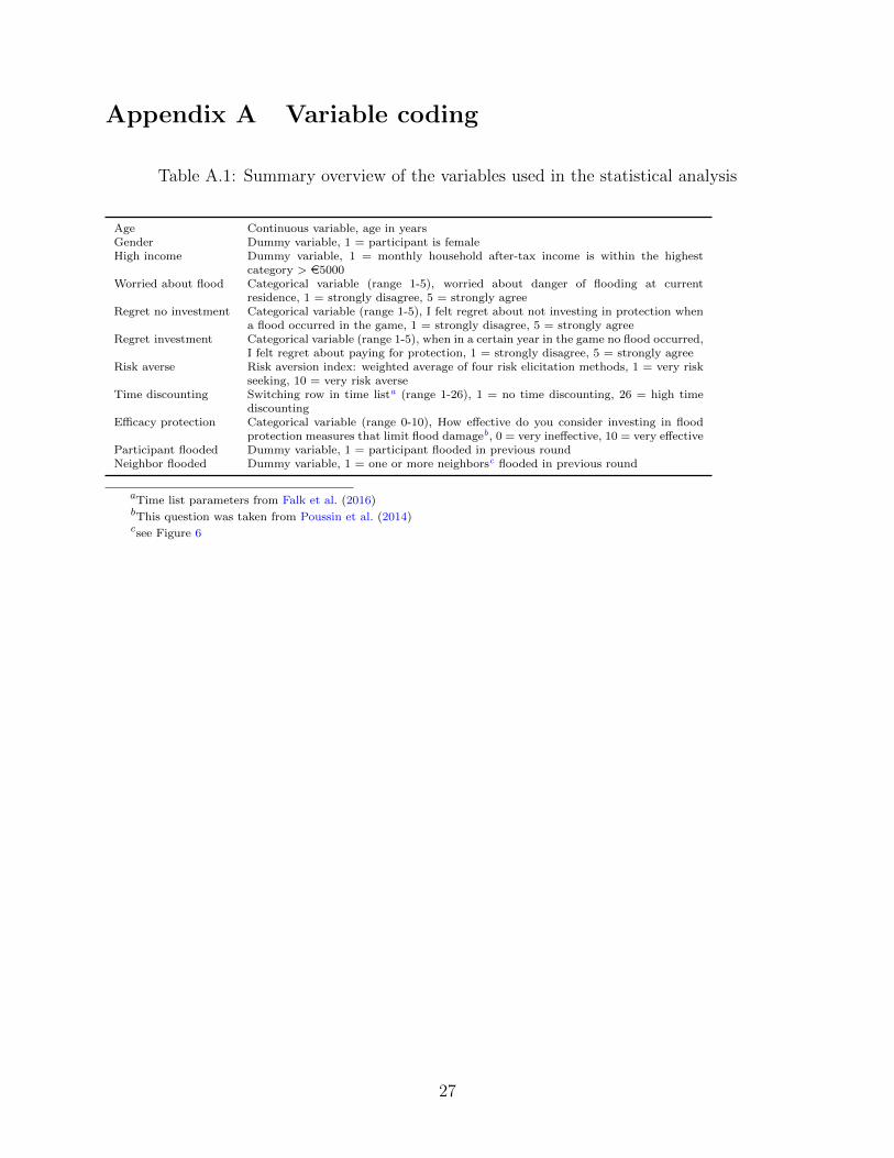
Table A.1: Summary overview of the variables used in the statistical analysis
Age Continuous variable, age in yearsGender Dummy variable, 1 = participant is femaleHigh income Dummy variable, 1 = monthly household after-tax income is within the highest
category > e5000Worried about flood Categorical variable (range 1-5), worried about danger of flooding at current
residence, 1 = strongly disagree, 5 = strongly agreeRegret no investment Categorical variable (range 1-5), I felt regret about not investing in protection when
a flood occurred in the game, 1 = strongly disagree, 5 = strongly agreeRegret investment Categorical variable (range 1-5), when in a certain year in the game no flood occurred,
I felt regret about paying for protection, 1 = strongly disagree, 5 = strongly agreeRisk averse Risk aversion index: weighted average of four risk elicitation methods, 1 = very risk
seeking, 10 = very risk averseTime discounting Switching row in time lista (range 1-26), 1 = no time discounting, 26 = high time
discountingEfficacy protection Categorical variable (range 0-10), How effective do you consider investing in flood
protection measures that limit flood damageb, 0 = very ineffective, 10 = very effectiveParticipant flooded Dummy variable, 1 = participant flooded in previous roundNeighbor flooded Dummy variable, 1 = one or more neighborsc flooded in previous round
aTime list parameters from Falk et al. (2016)bThis question was taken from Poussin et al. (2014)csee Figure 6
27

Appendix B Comparative statics
We aimed to derive theoretical predictions based on comparative statics for each of our
treatments. We start with the simplest case: the effect of insurance coverage, by comparing
the Insurance Baseline and the No Insurance treatments (Hypothesis 1).
Insurance Baseline versus No Insurance
Coverage α determines the difference between the Insurance Baseline and the No Insurance
treatments. We determine the optimal investment in mitigation r in relation to α. Taking
the derivative of Equation 2 with respect to r leads to the first order condition:
F = −(1− p)U ′[W1 − απ − r]− p((1− α)L′(r) + 1)U ′[W1 − απ − (1− α)L(r)− r)]
−p((1− α)L′(r))T∑t=2
1
(1 + δ)t−1
(U ′[Wt − απ − (1− α)L(r)]
)= 0
(B.1)
Using the implicit function theorem:
∂r
∂α= −F
′α
F ′r
Fulfilled second order condition implies:
F ′r < 0
Abbreviating W1−απ−r as nL1, W1−απ−(1−α)L(r)−r as L1 and Wt−απ−(1−α)L(r)
as Lt:
F ′α = (1− p)πU ′′(nL1)− p((1− α)L′(r) + 1)(L(r)− π)U ′′(L1) + L′(r)pU ′(L1)
+L′(r)pT∑t=2
1
(1 + δ)t−1U ′(Lt)− p((1− α)L′(r))
T∑t=2
1
(1 + δ)t−1(L(r)− π)U ′′(Lt)
(B.2)
If we assume 1 < |(1− α)L′(r)| and a concave utility function, F ′α is negative. Then:
∂r
∂α< 0 (B.3)
Under more insurance coverage, optimal investment in r decreases, which is part of Hypothesis
1.
28
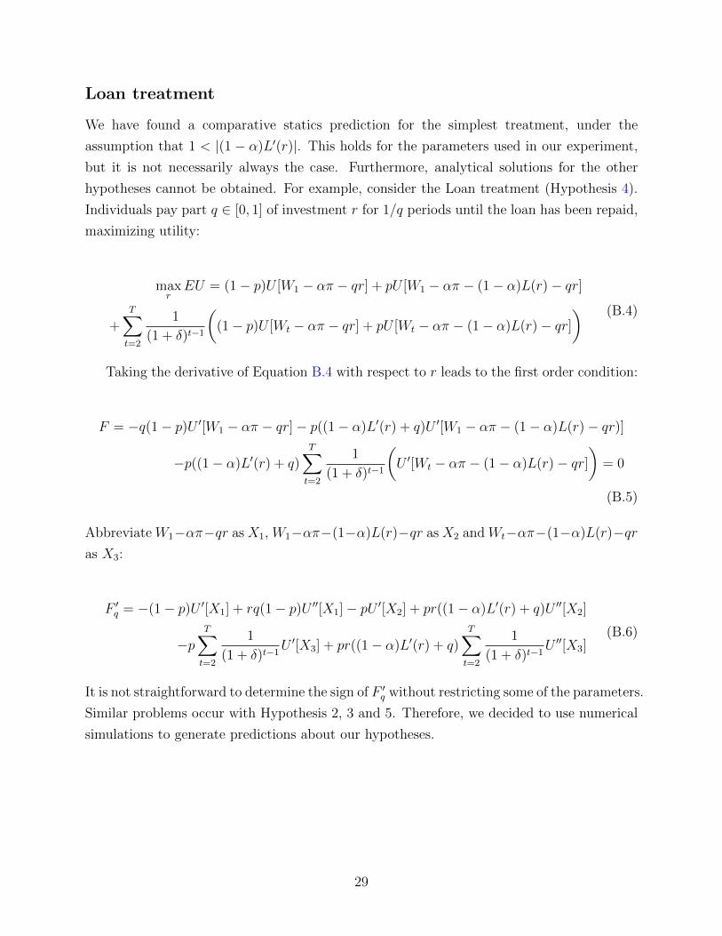
Loan treatment
We have found a comparative statics prediction for the simplest treatment, under the
assumption that 1 < |(1 − α)L′(r)|. This holds for the parameters used in our experiment,
but it is not necessarily always the case. Furthermore, analytical solutions for the other
hypotheses cannot be obtained. For example, consider the Loan treatment (Hypothesis 4).
Individuals pay part q ∈ [0, 1] of investment r for 1/q periods until the loan has been repaid,
maximizing utility:
maxrEU = (1− p)U [W1 − απ − qr] + pU [W1 − απ − (1− α)L(r)− qr]
+T∑t=2
1
(1 + δ)t−1
((1− p)U [Wt − απ − qr] + pU [Wt − απ − (1− α)L(r)− qr]
) (B.4)
Taking the derivative of Equation B.4 with respect to r leads to the first order condition:
F = −q(1− p)U ′[W1 − απ − qr]− p((1− α)L′(r) + q)U ′[W1 − απ − (1− α)L(r)− qr)]
−p((1− α)L′(r) + q)T∑t=2
1
(1 + δ)t−1
(U ′[Wt − απ − (1− α)L(r)− qr]
)= 0
(B.5)
Abbreviate W1−απ−qr as X1, W1−απ−(1−α)L(r)−qr as X2 and Wt−απ−(1−α)L(r)−qras X3:
F ′q = −(1− p)U ′[X1] + rq(1− p)U ′′[X1]− pU ′[X2] + pr((1− α)L′(r) + q)U ′′[X2]
−pT∑t=2
1
(1 + δ)t−1U ′[X3] + pr((1− α)L′(r) + q)
T∑t=2
1
(1 + δ)t−1U ′′[X3]
(B.6)
It is not straightforward to determine the sign of F ′q without restricting some of the parameters.
Similar problems occur with Hypothesis 2, 3 and 5. Therefore, we decided to use numerical
simulations to generate predictions about our hypotheses.
29

Appendix C Parameter calculations
To determine the parameters of our investment game, we calculated the net present value
(NPV) based on Expected Utility (Equation 2) for different combinations of parameters.
Some parameters were chosen based on estimations from reality, such as the maximum
damage (50,000 ECU) and the interest rate (1%). For the effectiveness of damage reducing
investments, we used the loss function L(r) = V e−βr proposed by Kelly and Kleffner (2003),
where V denotes the maximum loss and the effectiveness of mitigation is captured by
parameter β. We aimed to base our loss function on damage reduction estimates from
real data: Federal Emergency Management Agency (FEMA) cost estimates and damage
reduction estimates for a typical single family dwelling of flood mitigation measures. Figure
C.1 plots these estimates11 against the loss function with different values of β, with V =
200,000, the average value of this type of building. The mitigation function L(r) = V e−βr
with 0.00001 ≤ β ≤ 0.00008 seems to fit the data well.
Figure C.1: Parameter estimation of the mitigation function
We varied the parameters (savings account, income per round, probabilities, deductibles,
β, number of installments) to find a reasonable combination12 which allowed us to test
all our hypotheses. Table C.1 shows the results of these simulations with our final set of
parameters. The table displays the NPV of Expected Utility of investments in damage
mitigation over 12 rounds, discounted by δ = 0.01 for different degrees of risk aversion r
11Table 2.10, Table 2.13 and Table 2.18 from Aerts et al. (2013) to be precise.12For example: 0.00001 ≤ β ≤ 0.00008, positive income.
30

and normalized over the minimal and maximal possible expected values in the game. We
used a power utility function of the form u(x) = xr. The results are shown in comparison to
zero investment. Therefore all positive numbers are displayed in bold, as they indicate a net
gain from investing a positive amount. For each combination of treatment and scenario, the
largest positive number gives the optimal investment (underlined) for an individual. If no
number is underlined the optimal investment is zero. Table C.2 shows the results for high
discounting, δ = 0.1.
31

Table C.1: Normalized NPV of investment by scenario and treatment at δ = 0.01
(a) Risk averse (r = 0.3)
Insurance Baseline Premium Discount Loan Loan+Discount1,000 5,000 10,000 15,000 1,000 5,000 10,000 15,000 1,000 5,000 10,000 15,000 1,000 5,000 10,000 15,000
H - 0.030 0.124 0.198 0.239HH 0.009 0.025 0.008 -0.037 0.101 0.416 0.658 0.785 0.009 0.024 0.010 -0.028 0.101 0.415 0.659 0.794HL 0.002 -0.006 -0.042 -0.100 0.097 0.401 0.633 0.756 0.002 -0.005 -0.037 -0.086 0.097 0.401 0.638 0.768HxL -0.011 -0.059 -0.130 -0.212 0.092 0.376 0.594 0.708 -0.010 -0.056 -0.120 -0.189 0.092 0.380 0.604 0.728L - 0.002 0.003 -0.003 -0.017LH -0.011 -0.059 -0.128 -0.206 0.005 0.011 -0.012 -0.058 -0.010 -0.056 -0.118 -0.185 0.006 0.014 -0.002 -0.037LL -0.012 -0.064 -0.137 -0.217 0.005 0.010 -0.013 -0.059 -0.012 -0.061 -0.126 -0.195 0.006 0.013 -0.003 -0.038LxL -0.014 -0.074 -0.152 -0.237 0.005 0.008 -0.015 -0.062 -0.014 -0.070 -0.141 -0.214 0.005 0.012 -0.004 -0.039
(b) Risk neutral (r = 1)
Insurance Baseline Premium Discount Loan Loan+Discount1,000 5,000 10,000 15,000 1,000 5,000 10,000 15,000 1,000 5,000 10,000 15,000 1,000 5,000 10,000 15,000
H - 0.030 0.124 0.198 0.239HH 0.006 0.012 -0.012 -0.059 0.106 0.440 0.704 0.849 0.007 0.015 -0.005 -0.049 0.106 0.443 0.710 0.859HL 0.000 -0.015 -0.056 -0.116 0.106 0.440 0.704 0.849 0.000 -0.012 -0.050 -0.106 0.106 0.443 0.710 0.859HxL -0.013 -0.068 -0.146 -0.229 0.106 0.440 0.704 0.849 -0.012 -0.065 -0.139 -0.219 0.106 0.443 0.710 0.859L - 0.002 0.003 -0.003 -0.017LH -0.014 -0.074 -0.155 -0.240 0.006 0.012 -0.012 -0.059 -0.013 -0.071 -0.148 -0.231 0.007 0.015 -0.005 -0.049LL -0.015 -0.079 -0.164 -0.252 0.006 0.012 -0.012 -0.059 -0.015 -0.076 -0.157 -0.242 0.007 0.015 -0.005 -0.049LxL -0.018 -0.090 -0.182 -0.274 0.006 0.012 -0.012 -0.059 -0.017 -0.087 -0.175 -0.265 0.007 0.015 -0.005 -0.049
(c) Risk seeking (r = 3)
Insurance Baseline Premium Discount Loan Loan+Discount1,000 5,000 10,000 15,000 1,000 5,000 10,000 15,000 1,000 5,000 10,000 15,000 1,000 5,000 10,000 15,000
H - 0.030 0.124 0.198 0.239HH -0.005 -0.030 -0.070 -0.114 0.102 0.442 0.731 0.910 0.000 -0.012 -0.049 -0.104 0.107 0.460 0.754 0.921HL -0.008 -0.044 -0.094 -0.146 0.113 0.487 0.806 1.004 -0.004 -0.031 -0.083 -0.151 0.117 0.500 0.818 0.999HxL -0.018 -0.087 -0.169 -0.242 0.134 0.575 0.953 1.190 -0.016 -0.085 -0.180 -0.280 0.136 0.578 0.942 1.150L - 0.002 0.003 -0.003 -0.017LH -0.024 -0.116 -0.220 -0.314 0.006 0.014 -0.005 -0.043 -0.022 -0.114 -0.234 -0.358 0.008 0.015 -0.019 -0.087LL -0.025 -0.121 -0.229 -0.326 0.007 0.018 0.002 -0.035 -0.024 -0.120 -0.245 -0.373 0.009 0.019 -0.014 -0.082LxL -0.028 -0.133 -0.251 -0.354 0.009 0.025 0.012 -0.022 -0.027 -0.135 -0.272 -0.408 0.010 0.023 -0.009 -0.077
32
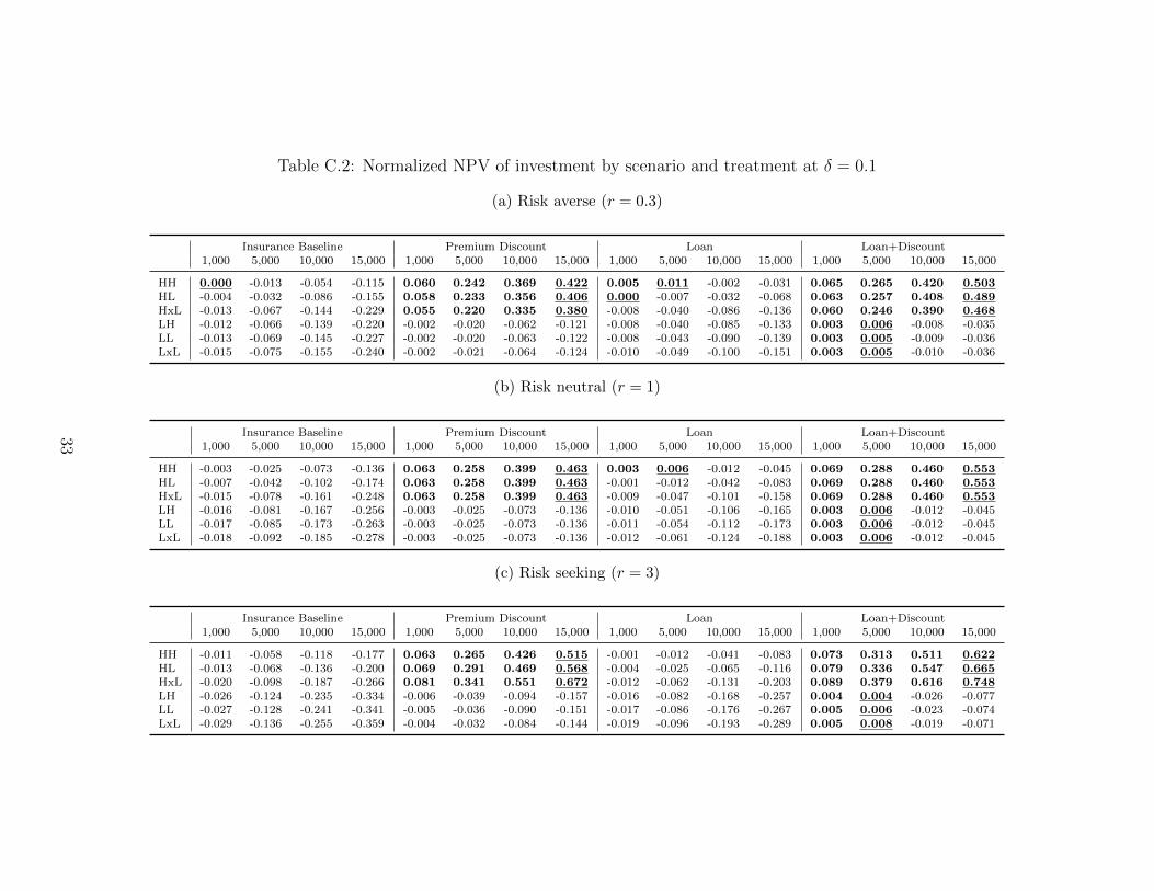
Table C.2: Normalized NPV of investment by scenario and treatment at δ = 0.1
(a) Risk averse (r = 0.3)
Insurance Baseline Premium Discount Loan Loan+Discount1,000 5,000 10,000 15,000 1,000 5,000 10,000 15,000 1,000 5,000 10,000 15,000 1,000 5,000 10,000 15,000
HH 0.000 -0.013 -0.054 -0.115 0.060 0.242 0.369 0.422 0.005 0.011 -0.002 -0.031 0.065 0.265 0.420 0.503HL -0.004 -0.032 -0.086 -0.155 0.058 0.233 0.356 0.406 0.000 -0.007 -0.032 -0.068 0.063 0.257 0.408 0.489HxL -0.013 -0.067 -0.144 -0.229 0.055 0.220 0.335 0.380 -0.008 -0.040 -0.086 -0.136 0.060 0.246 0.390 0.468LH -0.012 -0.066 -0.139 -0.220 -0.002 -0.020 -0.062 -0.121 -0.008 -0.040 -0.085 -0.133 0.003 0.006 -0.008 -0.035LL -0.013 -0.069 -0.145 -0.227 -0.002 -0.020 -0.063 -0.122 -0.008 -0.043 -0.090 -0.139 0.003 0.005 -0.009 -0.036LxL -0.015 -0.075 -0.155 -0.240 -0.002 -0.021 -0.064 -0.124 -0.010 -0.049 -0.100 -0.151 0.003 0.005 -0.010 -0.036
(b) Risk neutral (r = 1)
Insurance Baseline Premium Discount Loan Loan+Discount1,000 5,000 10,000 15,000 1,000 5,000 10,000 15,000 1,000 5,000 10,000 15,000 1,000 5,000 10,000 15,000
HH -0.003 -0.025 -0.073 -0.136 0.063 0.258 0.399 0.463 0.003 0.006 -0.012 -0.045 0.069 0.288 0.460 0.553HL -0.007 -0.042 -0.102 -0.174 0.063 0.258 0.399 0.463 -0.001 -0.012 -0.042 -0.083 0.069 0.288 0.460 0.553HxL -0.015 -0.078 -0.161 -0.248 0.063 0.258 0.399 0.463 -0.009 -0.047 -0.101 -0.158 0.069 0.288 0.460 0.553LH -0.016 -0.081 -0.167 -0.256 -0.003 -0.025 -0.073 -0.136 -0.010 -0.051 -0.106 -0.165 0.003 0.006 -0.012 -0.045LL -0.017 -0.085 -0.173 -0.263 -0.003 -0.025 -0.073 -0.136 -0.011 -0.054 -0.112 -0.173 0.003 0.006 -0.012 -0.045LxL -0.018 -0.092 -0.185 -0.278 -0.003 -0.025 -0.073 -0.136 -0.012 -0.061 -0.124 -0.188 0.003 0.006 -0.012 -0.045
(c) Risk seeking (r = 3)
Insurance Baseline Premium Discount Loan Loan+Discount1,000 5,000 10,000 15,000 1,000 5,000 10,000 15,000 1,000 5,000 10,000 15,000 1,000 5,000 10,000 15,000
HH -0.011 -0.058 -0.118 -0.177 0.063 0.265 0.426 0.515 -0.001 -0.012 -0.041 -0.083 0.073 0.313 0.511 0.622HL -0.013 -0.068 -0.136 -0.200 0.069 0.291 0.469 0.568 -0.004 -0.025 -0.065 -0.116 0.079 0.336 0.547 0.665HxL -0.020 -0.098 -0.187 -0.266 0.081 0.341 0.551 0.672 -0.012 -0.062 -0.131 -0.203 0.089 0.379 0.616 0.748LH -0.026 -0.124 -0.235 -0.334 -0.006 -0.039 -0.094 -0.157 -0.016 -0.082 -0.168 -0.257 0.004 0.004 -0.026 -0.077LL -0.027 -0.128 -0.241 -0.341 -0.005 -0.036 -0.090 -0.151 -0.017 -0.086 -0.176 -0.267 0.005 0.006 -0.023 -0.074LxL -0.029 -0.136 -0.255 -0.359 -0.004 -0.032 -0.084 -0.144 -0.019 -0.096 -0.193 -0.289 0.005 0.008 -0.019 -0.071
33

The following section repeats the hypotheses and explains briefly how each hypothesis
can be tested based on the predictions in Table C.1 and Table C.2.
Hypothesis 1 Damage reduction investments in the Insurance Baseline treatment are
lower than in the No Insurance treatment, but greater than zero. The NPV is higher for all
investments in No Insurance (denoted as H - and L - in Table C.1) compared to investments in
Insurance Baseline. In the high probability scenarios, positive investments may be optimal
with insurance, depending on the deductible level and attitude to risk. For example, for
a risk averse individual in scenario HH (Table C.1a) the optimal investment in Insurance
Baseline is 5,000 ECU, which leads to a positive NPV of 0.025 compared to no investment.
This allows for evaluation of Hypothesis 1.
Hypothesis 2 Risk-averse individuals will invest more in damage reduction in the Insurance
Baseline treatment and the Loan treatment than risk-neutral individuals, where risk-seeking
individuals will invest less. In the Insurance Baseline and the Loan treatment, risk-neutral
(r = 1, Table C.1b) individuals will invest 1,000 or 5,000 (HH) and 1,000 (HL). A risk-averse
individual (r = 0.3, Table C.1a) will also get a positive NPV for investing 10,000. Risk-seeking
individuals (r = 3, Table C.1c) will not invest in any of these scenarios.
Hypothesis 3 Damage reduction investments are higher in the Premium Discount treatment
than in the Insurance Baseline treatment. Comparing the Premium Discount column with
the Insurance Baseline column gives higher NPV values in each of the rows and sub-tables in
Table C.1. Therefore this hypothesis can be checked under all scenarios and risk attitudes.
Hypothesis 4 Damage reduction investments are lower for participants with high time
discount rates. This effect is strongest in the Insurance Baseline and Premium Discount
treatments, but disappears in the Loan and Loan+Discount treatments. In the Insurance
Baseline and Premium Discount treatments, increasing the time discount rate from little time
discounting (δ = 0.01 in Table C.1) to high time discounting (δ = 0.1 in Table C.2) decreases
the optimal investment level. No change can be seen in the Loan and Loan+Discount
treatments.
Hypothesis 5 Damage reduction investments are highest in the Loan+Discount treatment
Under little time discounting (Table C.1), investments in Premium Discount were already
optimal, such that they stay optimal in Loan+Discount. Under high time discounting (Table
C.2), Loan+Discount gives the highest optimal investments of all treatments in the low
probability scenarios.
34

Appendix D Comprehension questions
Correct answers are marked in bold.
Questions asked in all treatments
• What was the flood risk in the test scenario?
1%a) 3%b) 5%c) 10%d) 15%e) 20%f)
The answer depends on the risk in the test scenario (randomly determined).
• If you are flooded in year 1, what is the flood risk in year 2?
(a) Less than in year 1
(b) Flood risk does not change
(c) More than in year 1
• How long are protective investments effective?
(a) From the moment you implement to the end of the experiment
(b) From the moment you implement to the end of the scenario
(c) From the start of the scenario to the end of the scenario
Extra question in the No Insurance treatment
• What happens if you are flooded and you did not take protective investments?
(a) I have to pay the full damage: 50.000 ECU
(b) I have to pay a small fee
(c) I will cry
Extra question in all Insurance treatments
• What was your deductible (eigen risico) in the test scenario?
5 percenta) 15 percentb) 20 percentc) 50 percentd)
The answer depends on the deductible in the test scenario (randomly determined).
35

Extra question in the Loan and Loan+Discount treatments
• Should you always repay your loan?
(a) No, I can refuse to pay the loan cost
(b) No, if the loan is not fully repaid in the last year, I am lucky
(c) Yes, I will pay the loan cost in the first 5 years
(d) Yes, if the loan is not fully repaid in the last year, I will pay the remainder
Extra question in the Discount and Loan+Discount treatments
• What is the benefit of a protective investment?
(a) A reduced damage in case of a flood
(b) A lower premium
(c) Both reduced damage and a lower premium
(d) None of the above
36
Appendix E Additional analyses
Risk aversion index Our risk aversion index was a linear combination between the four
risk aversion measures, following Menkhoff and Sakha (2017). Table E.1 shows the results
of our random-effects ML panel regressions for each of the four measures separately, in
comparison to the combined measure (Model 5). All risk aversion measures except the price
list in the loss domain have positive and significant estimates.
37
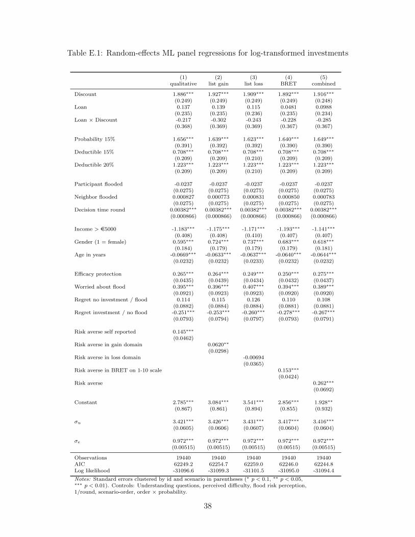
Table E.1: Random-effects ML panel regressions for log-transformed investments
(1) (2) (3) (4) (5)qualitative list gain list loss BRET combined
Discount 1.886∗∗∗ 1.927∗∗∗ 1.909∗∗∗ 1.892∗∗∗ 1.916∗∗∗
(0.249) (0.249) (0.249) (0.249) (0.248)Loan 0.137 0.139 0.115 0.0481 0.0988
(0.235) (0.235) (0.236) (0.235) (0.234)Loan × Discount -0.217 -0.302 -0.243 -0.228 -0.285
(0.368) (0.369) (0.369) (0.367) (0.367)
Probability 15% 1.656∗∗∗ 1.639∗∗∗ 1.623∗∗∗ 1.640∗∗∗ 1.649∗∗∗
(0.391) (0.392) (0.392) (0.390) (0.390)Deductible 15% 0.708∗∗∗ 0.708∗∗∗ 0.708∗∗∗ 0.708∗∗∗ 0.708∗∗∗
(0.209) (0.209) (0.210) (0.209) (0.209)Deductible 20% 1.223∗∗∗ 1.223∗∗∗ 1.223∗∗∗ 1.223∗∗∗ 1.223∗∗∗
(0.209) (0.209) (0.210) (0.209) (0.209)
Participant flooded -0.0237 -0.0237 -0.0237 -0.0237 -0.0237(0.0275) (0.0275) (0.0275) (0.0275) (0.0275)
Neighbor flooded 0.000827 0.000773 0.000831 0.000850 0.000783(0.0275) (0.0275) (0.0275) (0.0275) (0.0275)
Decision time round 0.00382∗∗∗ 0.00382∗∗∗ 0.00382∗∗∗ 0.00382∗∗∗ 0.00382∗∗∗
(0.000866) (0.000866) (0.000866) (0.000866) (0.000866)
Income > e5000 -1.183∗∗∗ -1.175∗∗∗ -1.171∗∗∗ -1.193∗∗∗ -1.141∗∗∗
(0.408) (0.408) (0.410) (0.407) (0.407)Gender (1 = female) 0.595∗∗∗ 0.724∗∗∗ 0.737∗∗∗ 0.683∗∗∗ 0.618∗∗∗
(0.184) (0.179) (0.179) (0.179) (0.181)Age in years -0.0669∗∗∗ -0.0633∗∗∗ -0.0637∗∗∗ -0.0640∗∗∗ -0.0644∗∗∗
(0.0232) (0.0232) (0.0233) (0.0232) (0.0232)
Efficacy protection 0.265∗∗∗ 0.264∗∗∗ 0.249∗∗∗ 0.250∗∗∗ 0.275∗∗∗
(0.0435) (0.0439) (0.0434) (0.0432) (0.0437)Worried about flood 0.395∗∗∗ 0.396∗∗∗ 0.407∗∗∗ 0.394∗∗∗ 0.389∗∗∗
(0.0921) (0.0923) (0.0923) (0.0920) (0.0920)Regret no investment / flood 0.114 0.115 0.126 0.110 0.108
(0.0882) (0.0884) (0.0884) (0.0881) (0.0881)Regret investment / no flood -0.251∗∗∗ -0.253∗∗∗ -0.260∗∗∗ -0.278∗∗∗ -0.267∗∗∗
(0.0793) (0.0794) (0.0797) (0.0793) (0.0791)
Risk averse self reported 0.145∗∗∗
(0.0462)Risk averse in gain domain 0.0620∗∗
(0.0298)Risk averse in loss domain -0.00694
(0.0365)Risk averse in BRET on 1-10 scale 0.153∗∗∗
(0.0424)Risk averse 0.262∗∗∗
(0.0692)
Constant 2.785∗∗∗ 3.084∗∗∗ 3.541∗∗∗ 2.856∗∗∗ 1.928∗∗
(0.867) (0.861) (0.894) (0.855) (0.932)
σu 3.421∗∗∗ 3.426∗∗∗ 3.431∗∗∗ 3.417∗∗∗ 3.416∗∗∗
(0.0605) (0.0606) (0.0607) (0.0604) (0.0604)
σe 0.972∗∗∗ 0.972∗∗∗ 0.972∗∗∗ 0.972∗∗∗ 0.972∗∗∗
(0.00515) (0.00515) (0.00515) (0.00515) (0.00515)
Observations 19440 19440 19440 19440 19440AIC 62249.2 62254.7 62259.0 62246.0 62244.8Log likelihood -31096.6 -31099.3 -31101.5 -31095.0 -31094.4
Notes: Standard errors clustered by id and scenario in parentheses (∗ p < 0.1, ∗∗ p < 0.05,∗∗∗ p < 0.01). Controls: Understanding questions, perceived difficulty, flood risk perception,1/round, scenario-order, order × probability.
38
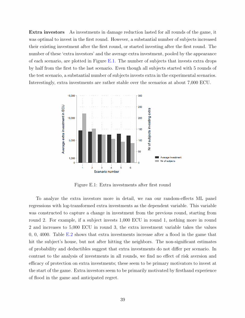
Extra investors As investments in damage reduction lasted for all rounds of the game, it
was optimal to invest in the first round. However, a substantial number of subjects increased
their existing investment after the first round, or started investing after the first round. The
number of these ‘extra investors’ and the average extra investment, pooled by the appearance
of each scenario, are plotted in Figure E.1. The number of subjects that invests extra drops
by half from the first to the last scenario. Even though all subjects started with 5 rounds of
the test scenario, a substantial number of subjects invests extra in the experimental scenarios.
Interestingly, extra investments are rather stable over the scenarios at about 7,000 ECU.
Figure E.1: Extra investments after first round
To analyze the extra investors more in detail, we ran our random-effects ML panel
regressions with log-transformed extra investments as the dependent variable. This variable
was constructed to capture a change in investment from the previous round, starting from
round 2. For example, if a subject invests 1,000 ECU in round 1, nothing more in round
2 and increases to 5,000 ECU in round 3, the extra investment variable takes the values
0, 0, 4000. Table E.2 shows that extra investments increase after a flood in the game that
hit the subject’s house, but not after hitting the neighbors. The non-significant estimates
of probability and deductibles suggest that extra investments do not differ per scenario. In
contrast to the analysis of investments in all rounds, we find no effect of risk aversion and
efficacy of protection on extra investments; these seem to be primary motivators to invest at
the start of the game. Extra investors seem to be primarily motivated by firsthand experience
of flood in the game and anticipated regret.
39
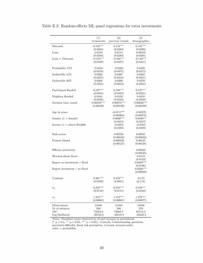
Table E.2: Random-effects ML panel regressions for extra investments
(1) (2) (3)treatments previous rounds demographics
Discount 0.132∗∗∗ 0.118∗∗∗ 0.145∗∗∗
(0.0284) (0.0284) (0.0298)Loan 0.0159 0.0115 0.00318
(0.0284) (0.0283) (0.0281)Loan × Discount -0.184∗∗∗ -0.166∗∗∗ -0.149∗∗∗
(0.0439) (0.0437) (0.0441)
Probability 15% -0.0318 -0.0262 0.0429(0.0478) (0.0475) (0.0472)
Deductible 15% 0.0386 0.0387 0.0383(0.0255) (0.0253) (0.0251)
Deductible 20% 0.0208 0.0209 0.0278(0.0255) (0.0253) (0.0251)
Participant flooded 0.197∗∗∗ 0.198∗∗∗ 0.197∗∗∗
(0.0344) (0.0343) (0.0351)Neighbor flooded 0.0164 0.0158 0.0216
(0.0343) (0.0342) (0.0350)Decision time round 0.00859∗∗∗ 0.00872∗∗∗ 0.00836∗∗∗
(0.00108) (0.00108) (0.00109)
Age in years -0.0111∗∗∗ -0.00270(0.00268) (0.00278)
Gender (1 = female) 0.0696∗∗∗ 0.0498∗∗
(0.0213) (0.0217)Income (1 = above e5,000) -0.0252 -0.0165
(0.0493) (0.0489)
Risk averse 0.00726 0.00521(0.00832) (0.00832)
Present biased 0.000933 0.00125(0.00127) (0.00128)
Efficacy protection 0.00848(0.00525)
Worried about flood 0.0119(0.0110)
Regret no investment / flood 0.0458∗∗∗
(0.0106)Regret investment / no flood 0.0426∗∗∗
(0.00950)
Constant 0.261∗∗∗ 0.419∗∗∗ -0.115(0.0530) (0.0951) (0.112)
σu 0.223∗∗∗ 0.216∗∗∗ 0.183∗∗∗
(0.0148) (0.0151) (0.0168)
σe 1.312∗∗∗ 1.312∗∗∗ 1.278∗∗∗
(0.00661) (0.00661) (0.00677)
Observations 21456 21456 19440Nr of subjects 298 298 270AIC 73104.3 73084.7 65112.4Log likelihood -36533.2 -36518.3 -32528.2
Notes: Standard errors clustered by id and scenario in parentheses(∗ p < 0.1, ∗∗ p < 0.05, ∗∗∗ p < 0.01). Controls: Understanding questions,perceived difficulty, flood risk perception, 1/round, scenario-order,order × probability.
40

screen shots of investment game - page 1/23
Screen shots of investment game

screen shots of investment game - page 2/23
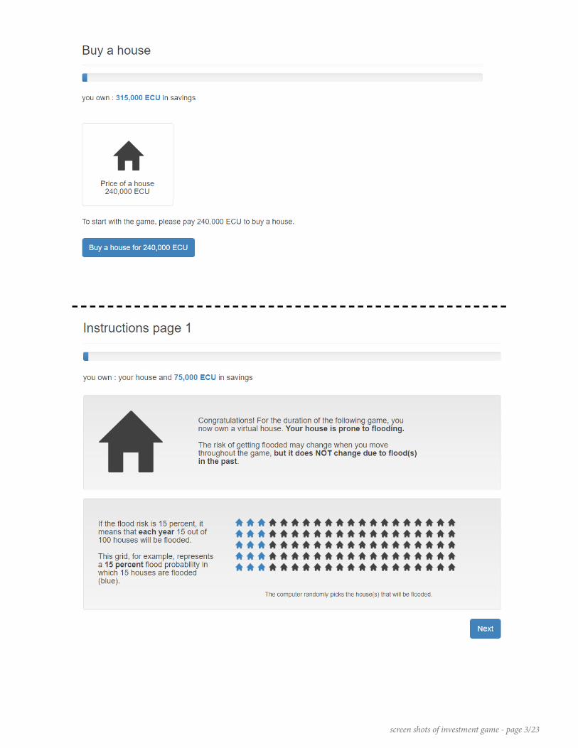
screen shots of investment game - page 3/23
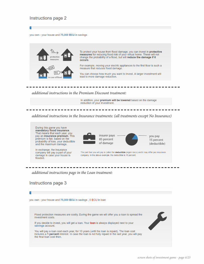
screen shots of investment game - page 4/23
additional instructions in the Insurance treatments: (all treatments except No Insurance)
additional instructions in the Premium Discount treatment:
additional instructions page in the Loan treatment:
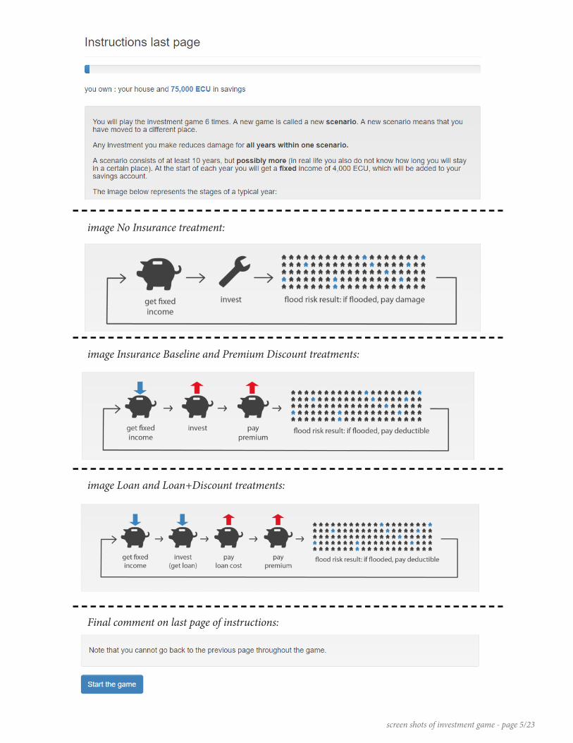
screen shots of investment game - page 5/23
image No Insurance treatment:
image Insurance Baseline and Premium Discount treatments:
image Loan and Loan+Discount treatments:
Final comment on last page of instructions:

screen shots of investment game - page 6/23
The test scenario contained the same page sequence as the final scenario. We excluded the Investment, Premium, Flood risk screenshots for brevity.

screen shots of investment game - page 7/23
Different banner at the start of scenario 2, 3, 4, 5 and 6:
Different text in insurance block in No Insurance treatment:

screen shots of investment game - page 8/23
Extra information in Insurance scenario:
Extra information in Premium Discount scenario:
Extra information in Loan scenario:

screen shots of investment game - page 9/23
Extra page in Loan scenario if participant decided to invest (in this example 1000 ECU):
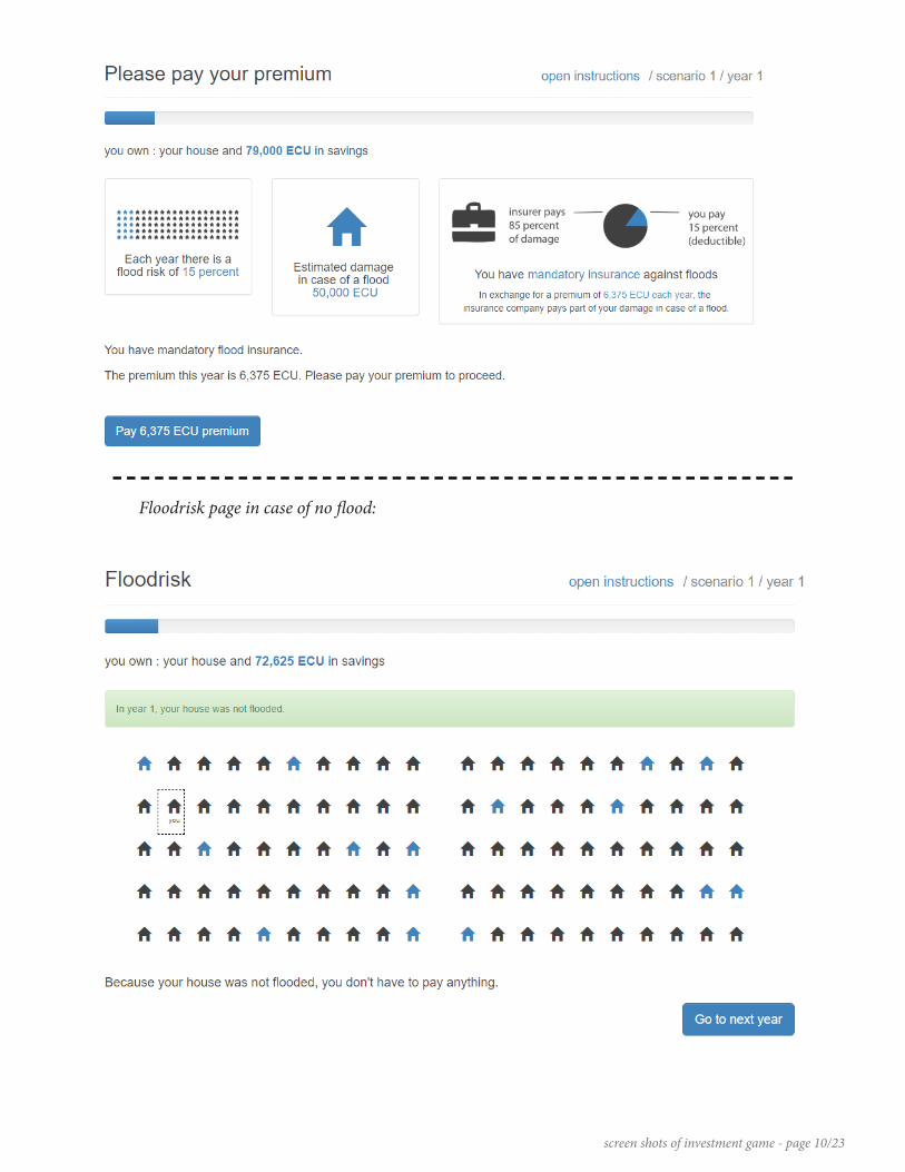
screen shots of investment game - page 10/23
Floodrisk page in case of no flood:
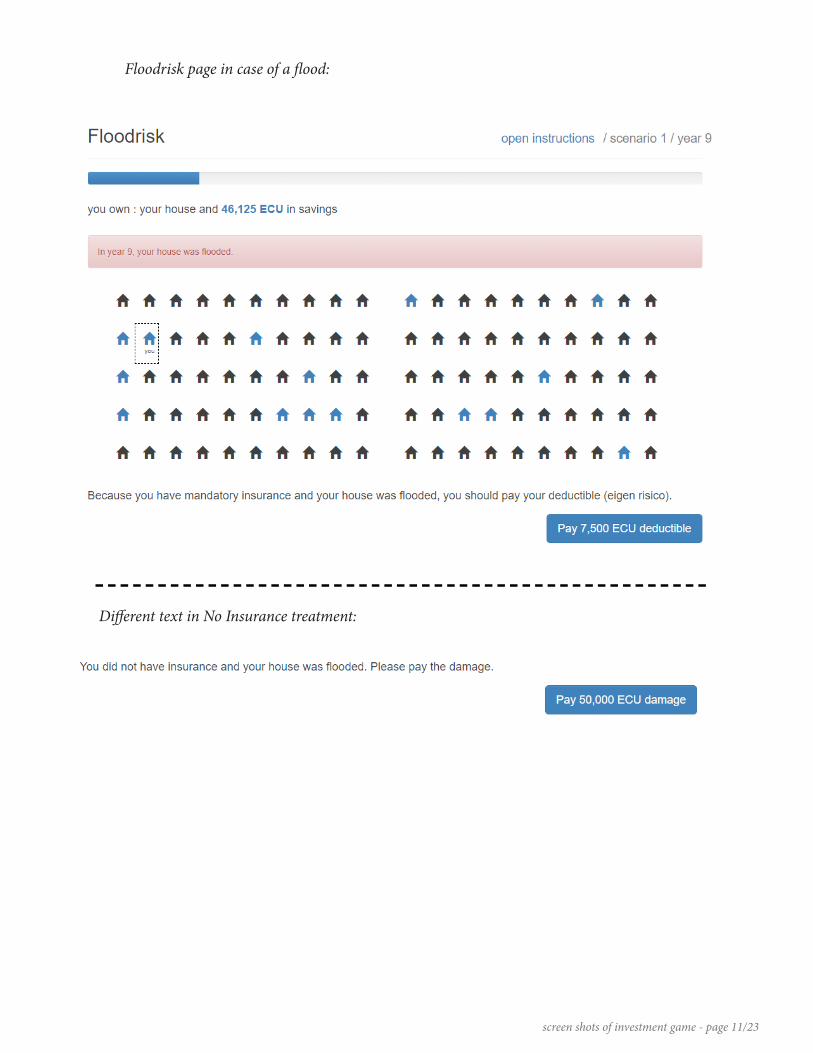
screen shots of investment game - page 11/23
Floodrisk page in case of a flood:
Different text in No Insurance treatment:
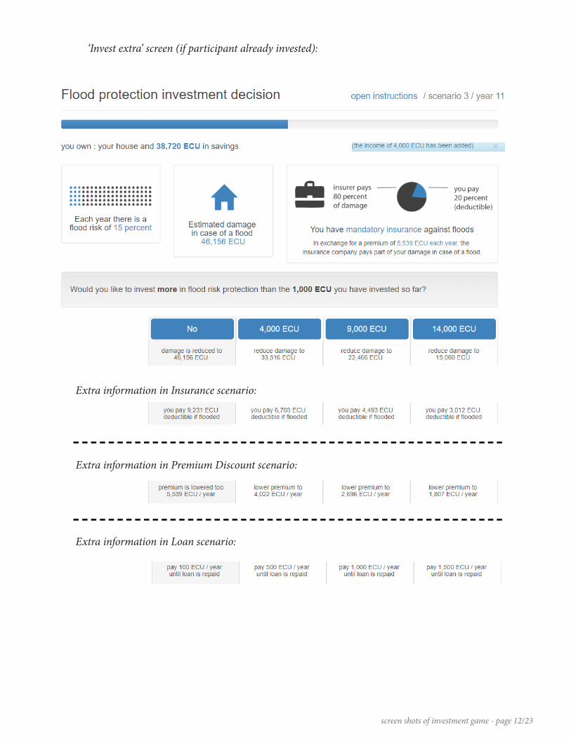
screen shots of investment game - page 12/23
‘Invest extra’ screen (if participant already invested):
Extra information in Insurance scenario:
Extra information in Premium Discount scenario:
Extra information in Loan scenario:

screen shots of investment game - page 13/23
At the end of the investment game (after 6 scenarios of 12 years each):
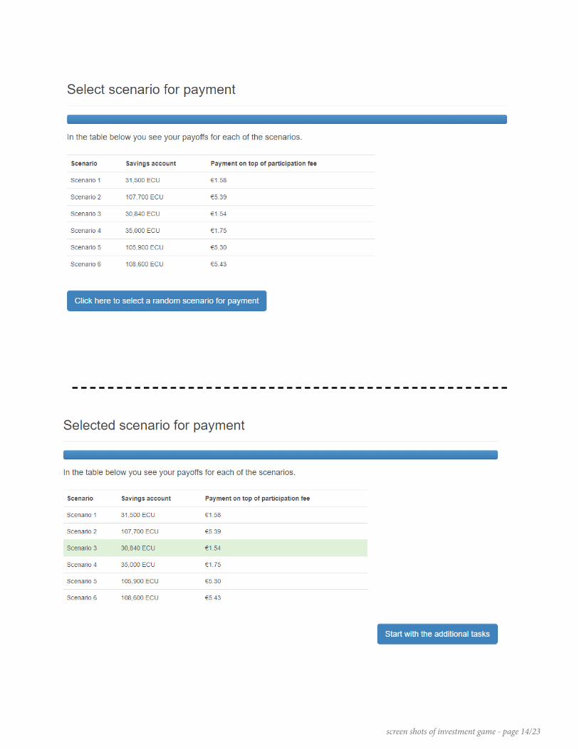
screen shots of investment game - page 14/23

screen shots of investment game - page 15/23

screen shots of investment game - page 16/23
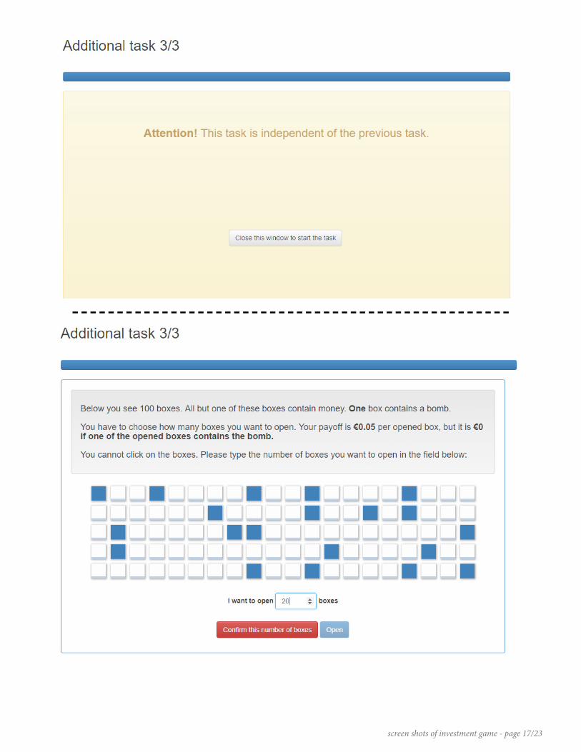
screen shots of investment game - page 17/23
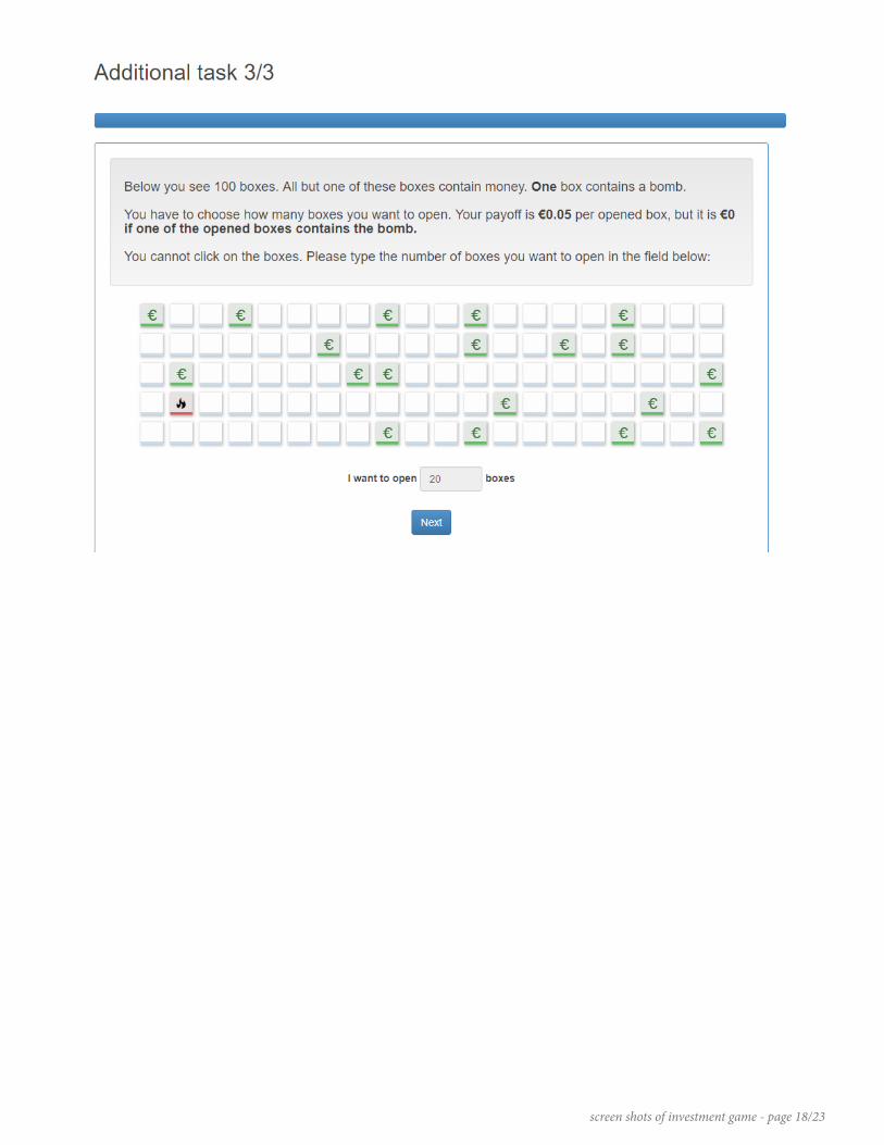
screen shots of investment game - page 18/23

screen shots of investment game - page 19/23

screen shots of investment game - page 20/23

screen shots of investment game - page 21/23

screen shots of investment game - page 22/23

screen shots of investment game - page 23/23


