
Statistical Computing with R – MATH 63821,∗
Set 5 (Monte Carlo Integration and VarianceReduction)
Tamer OrabyUTRGV
1Based on textbook.
∗Last updated November 2, 2016
Tamer Oraby (University of Texas RGV) SC MATH 6382 Fall 2016 1 / 56

Numerical Integration Deterministic Integration
Numerical Integration
Tamer Oraby (University of Texas RGV) SC MATH 6382 Fall 2016 2 / 56

Numerical Integration Deterministic Integration
Integration
The goal is to find the integral∫ b
a g(x)dx with possibly unboundedlimits
We know that∫ b
a 2xdx = b2 − a2, but we don’t know a closed formfor∫ b
a e−x2dx
Tamer Oraby (University of Texas RGV) SC MATH 6382 Fall 2016 3 / 56

Numerical Integration Deterministic Integration
1. Newton-Cotes Integration
If a,b <∞. The Newton-Cotes Integration of degree n∫ b
ag(x)dx ≈
n∑j=0
wjg(xj)
where the nodal points xj = a + j ∗ h, h =b − a
nand the weights are
the solution of1 1 1 · · · 1x0 x1 x2 · · · xnx2
0 x21 x2
2 · · · x2n
...xn
0 xn1 xn
2 · · · xnn
w0w1w2...
wn
= (b − a)
11213...1
n+1
Tamer Oraby (University of Texas RGV) SC MATH 6382 Fall 2016 4 / 56

Numerical Integration Deterministic Integration
1. Newton-Cotes Integration
If a,b <∞. The Newton-Cotes Integration of degree n∫ b
ag(x)dx ≈
n∑j=0
wjg(xj)
where the nodal points xj = a + j ∗ h, h =b − a
nand the weights are
the solution of
wj =
∫ b
aLj(x)dx
where Lj(x) =∏n
k=0,k 6=j(x − xk )
(xj − xk )
Tamer Oraby (University of Texas RGV) SC MATH 6382 Fall 2016 5 / 56

Numerical Integration Deterministic Integration
1. Newton-Cotes Integration
The error in the Newton-Cotes Integration of a functiong ∈ Cn+1[a,b] of degree n is∫ b
ag(x)dx −
n∑j=0
wjg(xj) =
hn+2g(n+1)(ξ)
nn+2(n + 1)!
∫ n
0t(t − 1) · · · (t − n)dt
if n is odd, where ξ ∈ (a,b).Thus, Newton-Cotes has a precision of n if n is odd as it integratespolynomials of degrees up to n exactly.
Tamer Oraby (University of Texas RGV) SC MATH 6382 Fall 2016 6 / 56

Numerical Integration Deterministic Integration
1. Newton-Cotes Integration
The error in the Newton-Cotes Integration of a functiong ∈ Cn+2[a,b] of degree n is∫ b
ag(x)dx −
n∑j=0
wjg(xj) =
hn+3g(n+2)(ξ)
nn+3(n + 2)!
∫ n
0t2(t − 1) · · · (t − n)dt
if n is even, where ξ ∈ (a,b).Thus, Newton-Cotes has a precision of n + 1 if n is even as itintegrates polynomials of degrees up to n + 1 exactly.
Tamer Oraby (University of Texas RGV) SC MATH 6382 Fall 2016 7 / 56
Numerical Integration Deterministic Integration
2. Gaussian Quadrature Integration
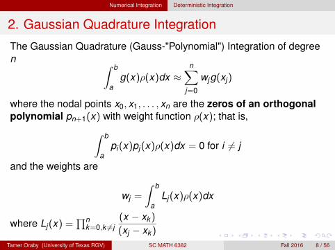
The Gaussian Quadrature (Gauss-"Polynomial") Integration of degreen ∫ b
ag(x)ρ(x)dx ≈
n∑j=0
wjg(xj)
where the nodal points x0, x1, . . . , xn are the zeros of an orthogonalpolynomial pn+1(x) with weight function ρ(x); that is,∫ b
api(x)pj(x)ρ(x)dx = 0 for i 6= j
and the weights are
wj =
∫ b
aLj(x)ρ(x)dx
where Lj(x) =∏n
k=0,k 6=j(x − xk )
(xj − xk )
Tamer Oraby (University of Texas RGV) SC MATH 6382 Fall 2016 8 / 56
Numerical Integration Deterministic Integration
2. Gaussian Quadrature Integration
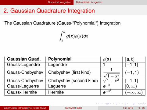
The Gaussian Quadrature (Gauss-"Polynomial") Integration∫ b
ag(x)ρ(x)dx
Gaussian Quad. Polynomial ρ(x) [a,b]Gauss-Legendre Legendre 1 [−1,1]
Gauss-Chebyshev Chebyshev (first kind)1√
1− x2(−1,1)
Gauss-Chebyshev Chebyshev (second kind)√
1− x2 [−1,1]Gauss-Laguerre Laguerre e−x [0,∞)
Gauss-Hermite Hermite e−x2(−∞,∞)
Tamer Oraby (University of Texas RGV) SC MATH 6382 Fall 2016 9 / 56
Numerical Integration Deterministic Integration
2. Gaussian Quadrature Integration
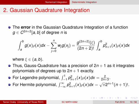
The error in the Gaussian Quadrature Integration of a functiong ∈ C2n+2[a,b] of degree n is∫ b
ag(x)ρ(x)dx −
n∑j=0
wjg(xj) =g(2n+2)(ξ)
(2n + 2)!
∫ b
ap2
n+1(x)ρ(x)dx
where ξ ∈ (a,b).Thus, Gauss-Quadrature has a precision of 2n + 1 as it integratespolynomials of degrees up to 2n + 1 exactly.
For Legendre polynomial,∫ 1−1 p2
n+1(x)ρ(x)dx = 22n+3 .
For Hermite polynomial,∫∞−∞ p2
n+1(x)ρ(x)dx =√π2n+1(n + 1)!.
Tamer Oraby (University of Texas RGV) SC MATH 6382 Fall 2016 10 / 56
Numerical Integration Deterministic Integration
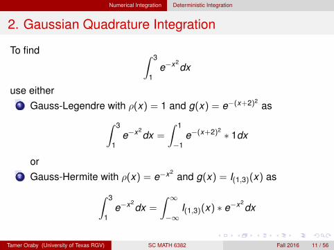
2. Gaussian Quadrature Integration
To find ∫ 3
1e−x2
dx
use either1 Gauss-Legendre with ρ(x) = 1 and g(x) = e−(x+2)2
as∫ 3
1e−x2
dx =
∫ 1
−1e−(x+2)2 ∗ 1dx
or2 Gauss-Hermite with ρ(x) = e−x2
and g(x) = I(1,3)(x) as∫ 3
1e−x2
dx =
∫ ∞−∞
I(1,3)(x) ∗ e−x2dx
Tamer Oraby (University of Texas RGV) SC MATH 6382 Fall 2016 11 / 56

Numerical Integration Deterministic Integration
Adaptive Quadrature Integration in R
To find∫ b
a g(x)dx useintegrate(function(x) g(x),a,b)
Example: Find∫ 1
0 2xdx> integrate(function(x) 2*x,0,1)1 with absolute error < 1.1e-14
Tamer Oraby (University of Texas RGV) SC MATH 6382 Fall 2016 12 / 56

Numerical Integration Monte Carlo Integration
Monte Carlo Integration
Tamer Oraby (University of Texas RGV) SC MATH 6382 Fall 2016 13 / 56
Numerical Integration Monte Carlo Integration
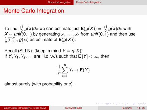
Monte Carlo Integration
To find∫ 1
0 g(x)dx we can estimate just E(g(X )) =∫ 1
0 g(x)dx withX ∼ unif (0,1) by generating x1, . . . , xn from unif (0,1) and then use1n∑n
i=1 g(xi) as estimate of E(g(X )).
Recall (SLLN): (keep in mind Y = g(X ))If Y ,Y1,Y2, . . . are i.i.d.r.v.’s such that E |Y | <∞, then
1n
n∑i=1
Yi → E(Y )
almost surely (with probability one).
Tamer Oraby (University of Texas RGV) SC MATH 6382 Fall 2016 14 / 56

Numerical Integration Monte Carlo Integration
Monte Carlo Integration
Remark:∫ ba g(x)dx = (b−a)
∫ 10 g(y(b−a)+a)dy ≈ (b−a) 1
n∑n
i=1 g(ui(b−a)+a)with u1, . . . ,un generated from unif (0,1)
OR∫ ba g(x)dx = (b − a)
∫ ba g(x) 1
b−adx ≈ (b − a) 1n∑n
i=1 g(xi) withx1, . . . , xn generated from unif (a,b)
Tamer Oraby (University of Texas RGV) SC MATH 6382 Fall 2016 15 / 56
Numerical Integration Monte Carlo Integration
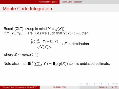
Monte Carlo Integration
Recall (CLT): (keep in mind Y = g(X ))If Y ,Y1,Y2, . . . are i.i.d.r.v.’s such that V(Y ) <∞, then
1n∑n
i=1 Yi − E(Y )√V(Y )/n
→ Z in distribution
where Z ∼ norm(0,1).
Note also, that E( 1n∑n
i=1 Yi) = EX (g(X )) so it is unbiased estimate.
Tamer Oraby (University of Texas RGV) SC MATH 6382 Fall 2016 16 / 56
Numerical Integration Monte Carlo Integration
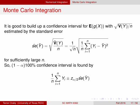
Monte Carlo Integration
It is good to build up a confidence interval for E(g(X )) with√
V(Y )/nestimated by the standard error
se(Y ) =
√V(Y )
n=
1√n
√√√√1n
n∑i=1
(Yi − Y )2
for sufficiently large n.So, (1− α)100% confidence interval is found by
1n
n∑i=1
Yi ± zα/2se(Y )
Tamer Oraby (University of Texas RGV) SC MATH 6382 Fall 2016 17 / 56

Numerical Integration Monte Carlo Integration
Monte Carlo Integration
Example: Estimate∫ 3
1 e−x2dx and find 95% confidence interval for that
integral. Remark:∫ 3
1 e−x2dx =
√πP(1 < X < 3) when X ∼ N(0, 1√
2)
andsqrt(pi)*(pnorm(3,0,1/sqrt(2))-pnorm(1,0,1/sqrt(2)))[1] 0.1393832
Tamer Oraby (University of Texas RGV) SC MATH 6382 Fall 2016 18 / 56

Numerical Integration Monte Carlo Integration
Monte Carlo Integration
First method:∫ 3
1e−x2
dx =
∫ 3
1(3− 1) ∗ e−x2 1
3− 1dx = EX ((3− 1) ∗ e−X 2
)
with X ∼ unif (1,3)n<-10000;CL<-.95x<-runif(n,1,3)y<-(3-1)*exp(-1*x2)mu1<-mean(y)mu1[1] 0.1363614se1<-sd(y)/sqrt(n)CI<-c(mu1-qnorm((1+CL)/2)*se1,mu1+qnorm((1+CL)/2)*se1)CI[1] 0.1326229 0.1401000
Tamer Oraby (University of Texas RGV) SC MATH 6382 Fall 2016 19 / 56
Numerical Integration Monte Carlo Integration
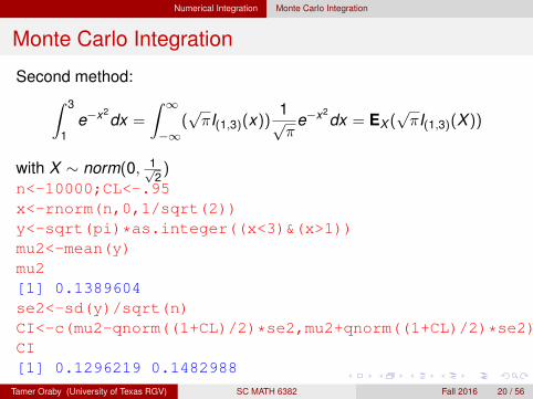
Monte Carlo Integration
Second method:∫ 3
1e−x2
dx =
∫ ∞−∞
(√πI(1,3)(x))
1√π
e−x2dx = EX (
√πI(1,3)(X ))
with X ∼ norm(0, 1√2
)n<-10000;CL<-.95x<-rnorm(n,0,1/sqrt(2))y<-sqrt(pi)*as.integer((x<3)&(x>1))mu2<-mean(y)mu2[1] 0.1389604se2<-sd(y)/sqrt(n)CI<-c(mu2-qnorm((1+CL)/2)*se2,mu2+qnorm((1+CL)/2)*se2)CI[1] 0.1296219 0.1482988
Tamer Oraby (University of Texas RGV) SC MATH 6382 Fall 2016 20 / 56

Numerical Integration Variance Reduction
Variance Reduction
Tamer Oraby (University of Texas RGV) SC MATH 6382 Fall 2016 21 / 56

Numerical Integration Variance Reduction
Efficiency
If θ1 and θ2 are two estimators of a parameter θ then θ1 is moreefficient than θ2 if
V(θ1) < V(θ2)
and the amount of reduction in variance is measured by
(V(θ1)− V(θ2))/V(θ1)
Note that computational efficiency is also implied.
Example: In the previous example θ1 = 0.1363614 andθ2 = 0.1389604 are two estimators of
∫ 31 e−x2
dxThe estimated amount of reduction in variance is(se12-se22)/se12[1] -5.31999
Tamer Oraby (University of Texas RGV) SC MATH 6382 Fall 2016 22 / 56

Numerical Integration Variance Reduction
VarianceReduction–Antithetic
Variables
Tamer Oraby (University of Texas RGV) SC MATH 6382 Fall 2016 23 / 56
Numerical Integration Variance Reduction
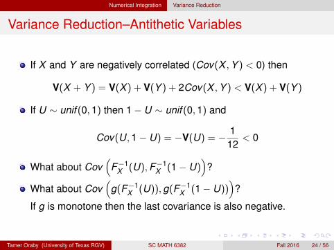
Variance Reduction–Antithetic Variables
If X and Y are negatively correlated (Cov(X ,Y ) < 0) then
V(X + Y ) = V(X ) + V(Y ) + 2Cov(X ,Y ) < V(X ) + V(Y )
If U ∼ unif (0,1) then 1− U ∼ unif (0,1) and
Cov(U,1− U) = −V(U) = − 112
< 0
What about Cov(
F−1X (U),F−1
X (1− U))
?
What about Cov(
g(F−1X (U)),g(F−1
X (1− U)))
?
If g is monotone then the last covariance is also negative.
Tamer Oraby (University of Texas RGV) SC MATH 6382 Fall 2016 24 / 56
Numerical Integration Variance Reduction
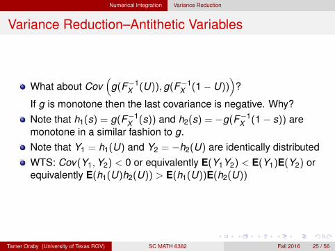
Variance Reduction–Antithetic Variables
What about Cov(
g(F−1X (U)),g(F−1
X (1− U)))
?
If g is monotone then the last covariance is negative. Why?Note that h1(s) = g(F−1
X (s)) and h2(s) = −g(F−1X (1− s)) are
monotone in a similar fashion to g.Note that Y1 = h1(U) and Y2 = −h2(U) are identically distributedWTS: Cov(Y1,Y2) < 0 or equivalently E(Y1Y2) < E(Y1)E(Y2) orequivalently E(h1(U)h2(U)) > E(h1(U))E(h2(U))
Tamer Oraby (University of Texas RGV) SC MATH 6382 Fall 2016 25 / 56

Numerical Integration Variance Reduction
Variance Reduction–Antithetic Variables
Assume WLOG that h1 and h2 are increasing, then for any x andy ∈ R
(h1(x)− h1(y))(h2(x)− h2(y)) ≥ 0
Let U1 and U2 are i.i.d.r.v.’s then
E ((h1(U1)− h1(U2))(h2(U1)− h2(U2))) ≥ 0
thusE ((h1(U1)h2(U1) + h1(U2)h2(U2)) ≥
E (h1(U2)h2(U1) + h1(U1)h2(U2))
hence, by independence and identical distribution of U1 and U2
E(h1(U1)h2(U1)) > E(h1(U1))E(h2(U1))
Tamer Oraby (University of Texas RGV) SC MATH 6382 Fall 2016 26 / 56
Numerical Integration Variance Reduction
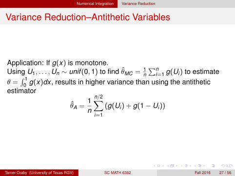
Variance Reduction–Antithetic Variables
Application: If g(x) is monotone.Using U1, . . . ,Un ∼ unif (0,1) to find θMC = 1
n∑n
i=1 g(Ui) to estimateθ =
∫ 10 g(x)dx , results in higher variance than using the antithetic
estimator
θA =1n
n/2∑i=1
(g(Ui) + g(1− Ui))
Tamer Oraby (University of Texas RGV) SC MATH 6382 Fall 2016 27 / 56

Numerical Integration Variance Reduction
Variance Reduction–Antithetic Variables
That is θA is more efficient than θMC . Since,
V(θA) =1n2
n/2∑i=1
V (g(Ui) + g(1− Ui)) by independence
=1
2nV (g(U) + g(1− U)) since identically distributed
=1
2n[V (g(U)) + V (g(1− U)) + 2Cov (g(U),g(1− U))]
≤ 12n
[V (g(U)) + V (g(1− U))]
≤ V(g(U))
n= V(θMC)
Tamer Oraby (University of Texas RGV) SC MATH 6382 Fall 2016 28 / 56

Numerical Integration Variance Reduction
Variance Reduction–Antithetic Variables
Note that V(θA) = 12n V (g(U) + g(1− U))
What aboutCov
(g(F−1
X (U1), . . . ,F−1X (Un)),g(F−1
X (1− U1), . . . ,F−1X (1− Un))
)?
If g is monotone then the last covariance is also negative. You canuse induction on n.
Tamer Oraby (University of Texas RGV) SC MATH 6382 Fall 2016 29 / 56
Numerical Integration Variance Reduction
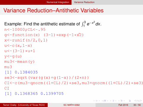
Variance Reduction–Antithetic Variables
Example: Find the antithetic estimate of∫ 3
1 e−x2dx .
n<-10000;CL<-.95g<-function(x) (3-1)*exp(-1*x2)x<-runif(n/2,0,1)u<-c(x,1-x)u<-(3-1)*u+1y<-g(u)mu3<-mean(y)mu3[1] 0.1384035se3<-sqrt(var(g(x)+g(1-x))/(2*n))CI<-c(mu3-qnorm((1+CL)/2)*se3,mu3+qnorm((1+CL)/2)*se3)CI[1] 0.1368365 0.1399705
Tamer Oraby (University of Texas RGV) SC MATH 6382 Fall 2016 30 / 56
Numerical Integration Variance Reduction
Variance Reduction–Antithetic Variables
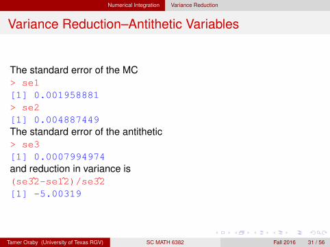
The standard error of the MC> se1[1] 0.001958881> se2[1] 0.004887449The standard error of the antithetic> se3[1] 0.0007994974and reduction in variance is(se32-se12)/se32[1] -5.00319
Tamer Oraby (University of Texas RGV) SC MATH 6382 Fall 2016 31 / 56

Numerical Integration Variance Reduction
Variance Reduction–ControlVariates
Tamer Oraby (University of Texas RGV) SC MATH 6382 Fall 2016 32 / 56

Numerical Integration Variance Reduction
Variance Reduction–Control Variates
A θC estimates θ = E(g(X )) via a control variate f (X ) with a knownµ = E(f (X )) for some function f , is given by
θC =1n
n∑i=1
(g(Xi) + c(f (Xi)− µ))
for some c, where X ,X1, . . . ,Xn are i.i.d.r.v.It is unbiased estimator since
E(θC) =1n
n∑i=1
E(g(Xi) + c(f (Xi)− µ)) = E(g(X )) + cE((f (X )− µ))
= E(g(X ))
To make it efficient
nV(θC) = V(g(X ) + c(f (X )− µ)) =
V(g(X )) + c2V(f (X )) + 2cCov(g(X ), f (X ))
Tamer Oraby (University of Texas RGV) SC MATH 6382 Fall 2016 33 / 56
Numerical Integration Variance Reduction
Variance Reduction–Control Variates
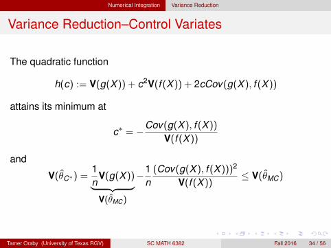
The quadratic function
h(c) := V(g(X )) + c2V(f (X )) + 2cCov(g(X ), f (X ))
attains its minimum at
c∗ = −Cov(g(X ), f (X ))
V(f (X ))
and
V(θC∗) =1n
V(g(X ))︸ ︷︷ ︸V(θMC)
−1n
(Cov(g(X ), f (X )))2
V(f (X ))≤ V(θMC)
Tamer Oraby (University of Texas RGV) SC MATH 6382 Fall 2016 34 / 56

Numerical Integration Variance Reduction
Variance Reduction–Control Variates
and the reduction in variance is given by
V(θMC)− V(θC∗)
V(θMC)=
(Cov(g(X ), f (X )))2
V(f (X ))V(g(X ))
= (Corr(g(X ), f (X )))2
so the higher the magnitude of correlation the higher is the reduction.
Tamer Oraby (University of Texas RGV) SC MATH 6382 Fall 2016 35 / 56

Numerical Integration Variance Reduction
Variance Reduction–Control Variates
Example: Find estimate of∫ 3
1 e−x2dx using control variate.
Here, let U ∼ unif (1,3) and so g(x) = 2e−x2. Let the control variate be
f (x) = x as it is easy to handle since µ = E(f (U)) = E(U) = 2 andV(f (U)) = V(U) = 1
3 . Then
θC∗ =1n
n∑i=1
(g(Ui) + c∗(f (Ui)− µ)) =1n
n∑i=1
(2e−U2
i + c∗(Ui − 2))
wherec∗ = −Cov(g(U), f (U))
V(f (U))=
−E(2Ue−U2)− E(2e−U2
)E(U)
1/3= 6 E(2e−U2
)︸ ︷︷ ︸estimated by θC∗
−32
(e−1 − e−9)
Tamer Oraby (University of Texas RGV) SC MATH 6382 Fall 2016 36 / 56

Numerical Integration Variance Reduction
Variance Reduction–Control Variates
Thus,
θC∗ =
1n∑n
i=1
(2e−U2
i − 32(e−1 − e−9)(Ui − 2)
)1− 6
n∑n
i=1(Ui − 2)
n<-10000;CL<-.95x<-runif(n,1,3)y<-mean(x)z<-mean(2*exp(-1*x2))mu4<-(z-(3/2)*(exp(-1)-exp(-9))*(y-2))/(1-6*(y-2))mu4[1] 0.1379537(cor(x,2*exp(-1*x2)))2[1] 0.7138062
Tamer Oraby (University of Texas RGV) SC MATH 6382 Fall 2016 37 / 56
Numerical Integration Variance Reduction
Variance Reduction–Control Variates
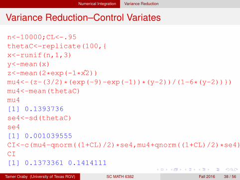
n<-10000;CL<-.95thetaC<-replicate(100,{x<-runif(n,1,3)y<-mean(x)z<-mean(2*exp(-1*x2))mu4<-(z-(3/2)*(exp(-9)-exp(-1))*(y-2))/(1-6*(y-2))})mu4<-mean(thetaC)mu4[1] 0.1393736se4<-sd(thetaC)se4[1] 0.001039555CI<-c(mu4-qnorm((1+CL)/2)*se4,mu4+qnorm((1+CL)/2)*se4)CI[1] 0.1373361 0.1414111
Tamer Oraby (University of Texas RGV) SC MATH 6382 Fall 2016 38 / 56

Numerical Integration Variance Reduction
Variance Reduction–Control Variates
The standard error of the MC> se1[1] 0.001958881> se2[1] 0.004887449The standard error of the antithetic> se3[1] 0.0007994974The standard error of the control variate> se4[1] 0.001039555and reduction in variance is(se12-se42)/se12[1] 0.7183699
Tamer Oraby (University of Texas RGV) SC MATH 6382 Fall 2016 39 / 56

Numerical Integration Variance Reduction
VarianceReduction–Importance
Sampling
Tamer Oraby (University of Texas RGV) SC MATH 6382 Fall 2016 40 / 56
Numerical Integration Variance Reduction
Variance Reduction–Importance Sampling
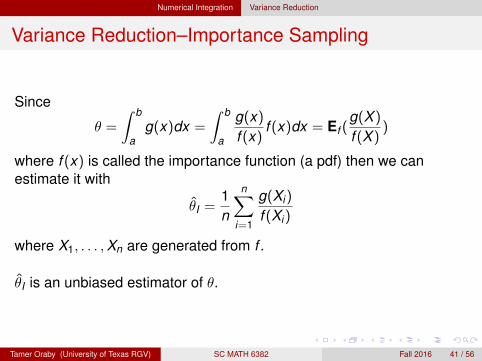
Since
θ =
∫ b
ag(x)dx =
∫ b
a
g(x)
f (x)f (x)dx = Ef (
g(X )
f (X ))
where f (x) is called the importance function (a pdf) then we canestimate it with
θI =1n
n∑i=1
g(Xi)
f (Xi)
where X1, . . . ,Xn are generated from f .
θI is an unbiased estimator of θ.
Tamer Oraby (University of Texas RGV) SC MATH 6382 Fall 2016 41 / 56
Numerical Integration Variance Reduction
Variance Reduction–Importance Sampling
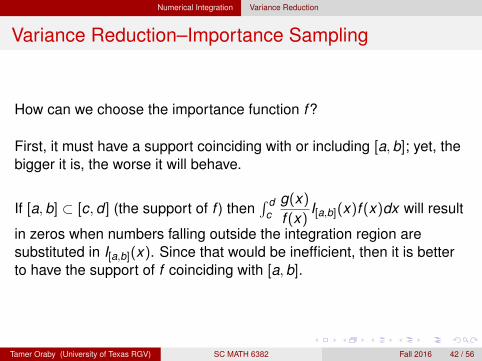
How can we choose the importance function f?
First, it must have a support coinciding with or including [a,b]; yet, thebigger it is, the worse it will behave.
If [a,b] ⊂ [c,d ] (the support of f ) then∫ d
cg(x)
f (x)I[a,b](x)f (x)dx will result
in zeros when numbers falling outside the integration region aresubstituted in I[a,b](x). Since that would be inefficient, then it is betterto have the support of f coinciding with [a,b].
Tamer Oraby (University of Texas RGV) SC MATH 6382 Fall 2016 42 / 56

Numerical Integration Variance Reduction
Variance Reduction–Importance Sampling
Second, V(θI) = 1n Vf (
g(X )
f (X )) which is the smallest possible if
g(x)
f (x)is
nearly a constant as the variability in a constant is zero.
The minimum is reached at f (x) =|g(x)|∫ b
a |g(t)|dtthat is a pdf.
Tamer Oraby (University of Texas RGV) SC MATH 6382 Fall 2016 43 / 56

Numerical Integration Variance Reduction
Variance Reduction–Importance Sampling
Example: Find estimate of∫ 3
1 e−x2dx using importance sampling.
Here we will compare several importance functions includingf0(x) = 1
2 , for 1 < x < 3 (MC Integration)f1(x) = e−x , for 0 < x <∞ (Wider domain)f2(x) = 2e−2x , for 0 < x <∞ (Wider domain)f3(x) = .5e−.5x , for 0 < x <∞ (Wider domain)f4(x) = 1
e−1−e−3 e−x , for 1 < x < 3f5(x) = 15
263(1− x2 + x4/2) , for 1 < x < 3
Tamer Oraby (University of Texas RGV) SC MATH 6382 Fall 2016 44 / 56
Numerical Integration Variance Reduction
Variance Reduction–Importance Sampling
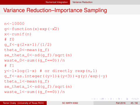
n<-10000g<-function(x)exp(-x2)x<-runif(n)# f0g_f<-g(2*x+1)/(1/2)theta_0<-mean(g_f)se_theta_0<-sd(g_f)/sqrt(n)waste_0<-sum((g_f==0))/n# f1y<-1*log(1-x) # or directly rexp(n,1)g_f<-as.integer((y>1)&(y<3))*g(y)/exp(-y)theta_1<-mean(g_f)se_theta_1<-sd(g_f)/sqrt(n)waste_1<-sum((g_f==0))/n
Tamer Oraby (University of Texas RGV) SC MATH 6382 Fall 2016 45 / 56

Numerical Integration Variance Reduction
Variance Reduction–Importance Sampling
# f2y<-.5*log(1-x) # or directly rexp(n,2)g_f<-as.integer((y>1)&(y<3))*g(y)/(2*exp(-2*y))theta_2<-mean(g_f)se_theta_2<-sd(g_f)/sqrt(n)waste_2<-sum((g_f==0))/n# f3y<-2*log(1-x) # or directly rexp(n,.5)g_f<-as.integer((y>1)&(y<3))*g(y)/(.5*exp(-.5*y))theta_3<-mean(g_f)se_theta_3<-sd(g_f)/sqrt(n)waste_3<-sum((g_f==0))/n
Tamer Oraby (University of Texas RGV) SC MATH 6382 Fall 2016 46 / 56

Numerical Integration Variance Reduction
Variance Reduction–Importance Sampling
# f4c<-exp(-1)-exp(-3)y<-1*log(exp(-1)-c*x)g_f<-g(y)/((1/c)*exp(-1*y))theta_4<-mean(g_f)se_theta_4<-sd(g_f)/sqrt(n)waste_4<-sum((g_f==0))/n# f5c<-15/263InvF<-function(x){uniroot(function(y)(c*(y-y3/3+y5/10-23/30)- x),lower=1,upper=3)$root}xv<-as.array(x)y<-apply(xv,1,InvF)g_f<-g(y)/(c*(1-y2+y4/2))theta_5<-mean(g_f)se_theta_5<-sd(g_f)/sqrt(n)
Tamer Oraby (University of Texas RGV) SC MATH 6382 Fall 2016 47 / 56

Numerical Integration Variance Reduction
Variance Reduction–Importance Sampling
waste_5<-sum((g_f==0))/nresult<-rbind(c(theta_0,theta_1,theta_2,theta_3,theta_4,theta_5),c(se_theta_0,se_theta_1,se_theta_2,se_theta_3,se_theta_4,se_theta_5),c(waste_0,waste_1,waste_2,waste_3,waste_4,waste_5))result<-as.data.frame(result,row.names=c("theta","se-theta","Waste"))colnames(result)<-c("f0","f1","f2","f3","f4","f5")result
f0 f1 f2 f3 f4 f5theta 0.139417213 0.137480914 0.138070629 0.141256850 0.140172414 0.124605248se-theta 0.001922774 0.002727444 0.003787346 0.002919893 0.001033504 0.008143972
Waste 0.000000000 0.685200000 0.868600000 0.615200000 0.000000000 0.000000000
Tamer Oraby (University of Texas RGV) SC MATH 6382 Fall 2016 48 / 56

Numerical Integration Variance Reduction
VarianceReduction–Stratified
Sampling
Tamer Oraby (University of Texas RGV) SC MATH 6382 Fall 2016 49 / 56
Numerical Integration Variance Reduction
Variance Reduction–Stratified Sampling
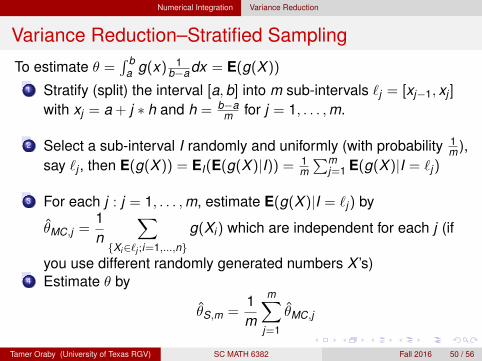
To estimate θ =∫ b
a g(x) 1b−adx = E(g(X ))
1 Stratify (split) the interval [a,b] into m sub-intervals `j = [xj−1, xj ]
with xj = a + j ∗ h and h = b−am for j = 1, . . . ,m.
2 Select a sub-interval I randomly and uniformly (with probability 1m ),
say `j , then E(g(X )) = EI(E(g(X )|I)) = 1m∑m
j=1 E(g(X )|I = `j)
3 For each j : j = 1, . . . ,m, estimate E(g(X )|I = `j) by
θMC,j =1n
∑{Xi∈`j ;i=1,...,n}
g(Xi) which are independent for each j (if
you use different randomly generated numbers X ’s)4 Estimate θ by
θS,m =1m
m∑j=1
θMC,j
Tamer Oraby (University of Texas RGV) SC MATH 6382 Fall 2016 50 / 56

Numerical Integration Variance Reduction
Variance Reduction–Stratified Sampling
WTS: V(θS,m) < V(θMC)
V(θS,m) = V(1m
m∑j=1
θMC,j)
=1
m2
m∑j=1
V(θMC,j) by independence
=1
m2
m∑j=1
V(g(X )|I = `j)
n
=1
mnE(V(g(X )|I))
≤ 1mn
V(g(X )) = V(θMC) since mn data points are used
Tamer Oraby (University of Texas RGV) SC MATH 6382 Fall 2016 51 / 56

Numerical Integration Variance Reduction
Variance Reduction–Stratified Sampling
n<-10000;a<-1;b<-3g<-function(x){(b-a)*exp(-x2)}gx<-g(runif(n,a,b))theta_MC<-mean(gx)se_theta_MC<-sd(gx)/sqrt(n)m<-4L<-seq(a,b,length=m+1)theta_MCJ<-c()for (j in 1:m){theta_MCJ[j]<-mean(g(runif(n/m,L[j],L[j+1])))
}theta_S<-mean(theta_MCJ)c(theta_MC,theta_S)[1] 0.1391709 0.1400730
Tamer Oraby (University of Texas RGV) SC MATH 6382 Fall 2016 52 / 56

Numerical Integration Variance Reduction
Variance Reduction–Stratified Sampling
n<-10000;a<-1;b<-3;m<-4;N<-1000g<-function(x){(b-a)*exp(-x2)}L<-seq(a,b,length=m+1)Vtheta_S<-matrix(0,N,2)for(i in 1:N){gx<-g(runif(n,a,b))Vtheta_S[i,1]<-mean(gx)theta_MCJ<-c()for (j in 1:m){theta_MCJ[j]<-mean(g(runif(n/m,L[j],L[j+1]))) }Vtheta_S[i,2]<-mean(theta_MCJ) }
apply(Vtheta_S,2,mean)[1] 0.1393923 0.1393566apply(Vtheta_S,2,sd)[1] 0.0019811043 0.0008233142
Tamer Oraby (University of Texas RGV) SC MATH 6382 Fall 2016 53 / 56
Numerical Integration Variance Reduction
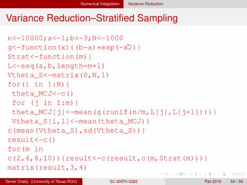
Variance Reduction–Stratified Sampling
n<-10000;a<-1;b<-3;N<-1000g<-function(x){(b-a)*exp(-x2)}Strat<-function(m){L<-seq(a,b,length=m+1)Vtheta_S<-matrix(0,N,1)for(i in 1:N){theta_MCJ<-c()for (j in 1:m){theta_MCJ[j]<-mean(g(runif(n/m,L[j],L[j+1])))}Vtheta_S[i,1]<-mean(theta_MCJ)}
c(mean(Vtheta_S),sd(Vtheta_S))}result<-c()for(m inc(2,4,8,10)){result<-c(result,c(m,Strat(m)))}matrix(result,3,4)
Tamer Oraby (University of Texas RGV) SC MATH 6382 Fall 2016 54 / 56

Numerical Integration Variance Reduction
Variance Reduction–Stratified Sampling
[,1] [,2] [,3] [,4][1,] 2.000000000 4.0000000000 8.000000000 1.000000e+01[2,] 0.139370017 0.1393186015 0.139409651 1.393670e-01[3,] 0.001497508 0.0007902412 0.000396519 3.229227e-04
Tamer Oraby (University of Texas RGV) SC MATH 6382 Fall 2016 55 / 56

Numerical Integration Variance Reduction
End of Set 5
Tamer Oraby (University of Texas RGV) SC MATH 6382 Fall 2016 56 / 56


