
1
Part 3 Process and Supply Chain Operations
Supply chain optimization
Jose Pinto
Appendices Demand ForecastTransportation IssuesThe Role of Inventory

2
Forecasting (uncertainty) Order service (certainty)
Demand management
Demand-Management Activities
RULE: Do not forecast what you can plan, calculate, or extract from supply chain feedback.
Source: Adapted from Plossl, “Getting the Most from Forecasts,” APICS 15th International Conference Proceedings, 1972

3
Strategies for satisfying customers(Types of Products )Make-to-Stock Product shipped from finished
goods, “off the shelf” (Examples)
Concerns What to stockInventory costsStock distribution
Make-to-Order Production initiated after receiptof customer order (Examples)
Concerns Efficient Manufacturing/PurchasingProduction schedulesFlexible facilities
4
Assemble-to-Order A make-to-order item wheresome or all components used inassembly, packaging and finishing processes are plannedand stocked in anticipation of a customer order (Examples)
Concerns What/ How many assemblies to stockRapid deliveryCustomized variations
Types of Products — Continued
Source: Adapted from Putnam and Wheeler, “Customer Service,” 1987.

5
Customer Service Policy IssuesOrder Responsiveness
Volume of order backlog
Service level
Order lead time required
Order Scheduling
Customer priority rules
Resource allocation
Product Substitution or UpgradeSource: Adapted from Forgarty et al., Production and Operations Management, 1989

6
Forecasts always wrongExpected value and measure of error
Long term less precise than short term
More accurate at the aggregate levelExample: monthly vs daily expenditure
The further up the supply chain a company is, the less accurate
Bullwhip effect
Determining demand - Forecasting
7
Qualitative Management reviewDelphi methodMarket research
QuantitativeMoving averageWeighted moving averageExponential smoothingRegression analysisPyramid
Forecasting - Main techniques
8
QualitativeUseful on new products: little historical dataAs a supplement to quantitative numbersSubjective
QuantitativeNeeds historical data or projected dataAvailableConsistentAccurateUnits - measurable
Forecasting
9
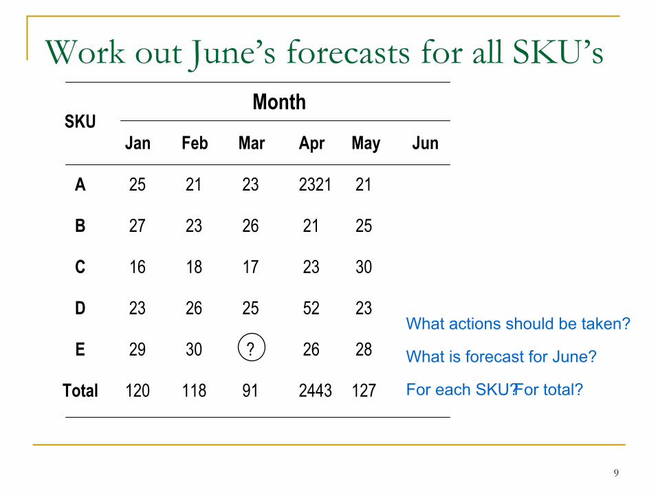
Work out June’s forecasts for all SKU’sMonth
SKUJan Feb Mar Apr May Jun
A 25 21 23 2321 21
B 27 23 26 21 25
C 16 18 17 23 30
D 23 26 25 52 23
E 29 30 ? 26 28
Total 120 118 91 2443 127
What actions should be taken?
What is forecast for June?
For each SKU? For total?

10
Simple Moving Averages
Simple Moving Average (SMA)
Forecast ForecastDemand (3-period) (4-period)180 start-up start-up160220200 186.6260 193.3 190240 226.6 210
233.3 230
Where F = Forecast T = Current time periodD = Demand n = Number of periods (max)
n
DDDF 2T1TT
1T
--+
++=
+ …
11
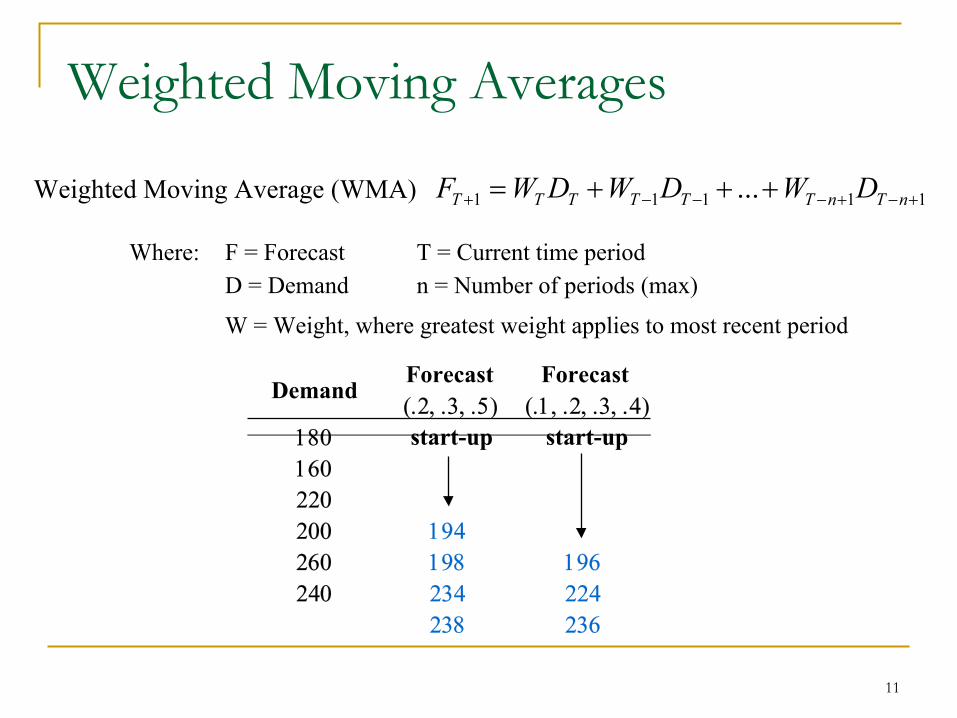
Weighted Moving Averages
Weighted Moving Average (WMA)
Where: F = Forecast T = Current time periodD = Demand n = Number of periods (max)
W = Weight, where greatest weight applies to most recent period
Forecast ForecastDemand
(.2, .3, .5) (.1, .2, .3, .4)180 start-up start-up160220200 194260 198 196240 234 224
238 236
1 1 1 1 1...T T T T T T n T nF W D W D W D+ − − − + − += + + +
12
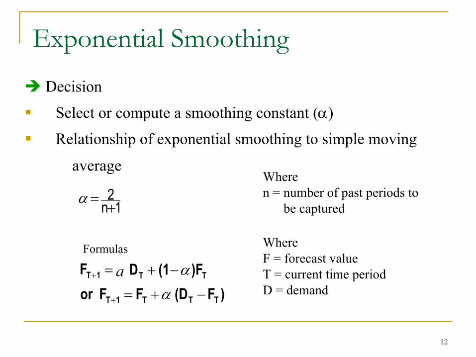
Exponential Smoothing
1n2+
=α
Decision
Select or compute a smoothing constant (α)
Relationship of exponential smoothing to simple moving
averageWheren = number of past periods to
be captured
WhereF = forecast valueT = current time periodD = demand
F 1T =+
Formulas
)F(DFF or TTT1T −+=+ α)F(1D TT −+ αa
13
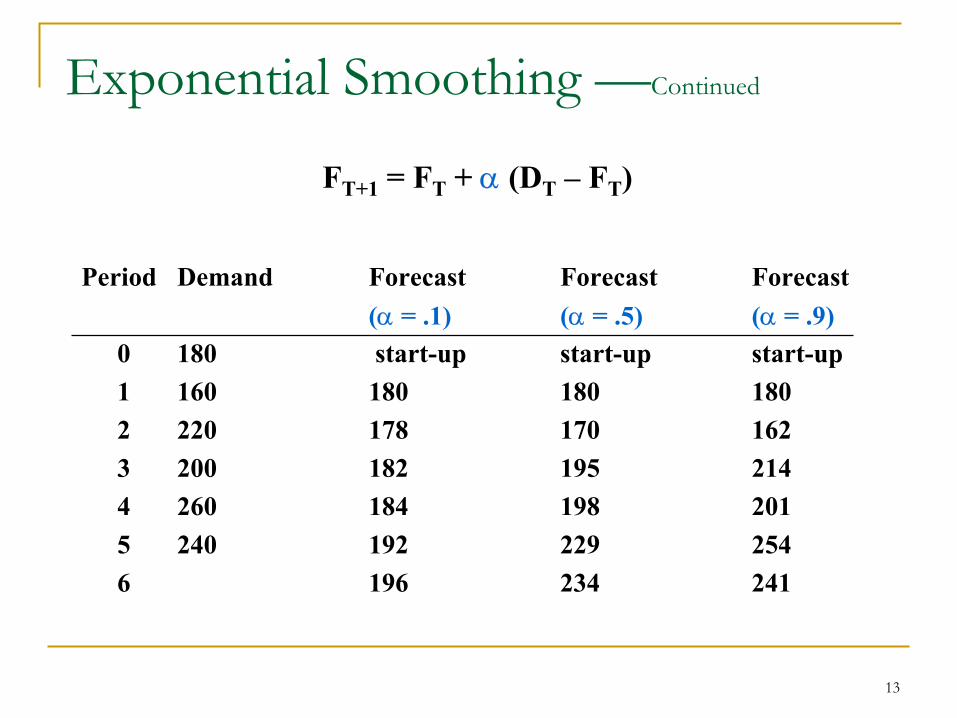
Period Demand Forecast Forecast Forecast(α = .1) (α = .5) (α = .9)
0 180 start-up start-up start-up1 160 180 180 1802 220 178 170 1623 200 182 195 2144 260 184 198 2015 240 192 229 2546 196 234 241
Exponential Smoothing —Continued
FT+1 = FT + α (DT – FT)
14
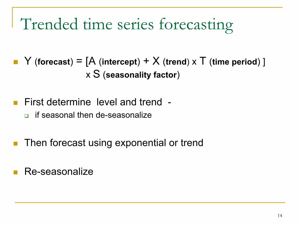
Trended time series forecasting
Y (forecast) = [A (intercept) + X (trend) x T (time period) ] x S (seasonality factor)
First determine level and trend -if seasonal then de-seasonalize
Then forecast using exponential or trend
Re-seasonalize
15
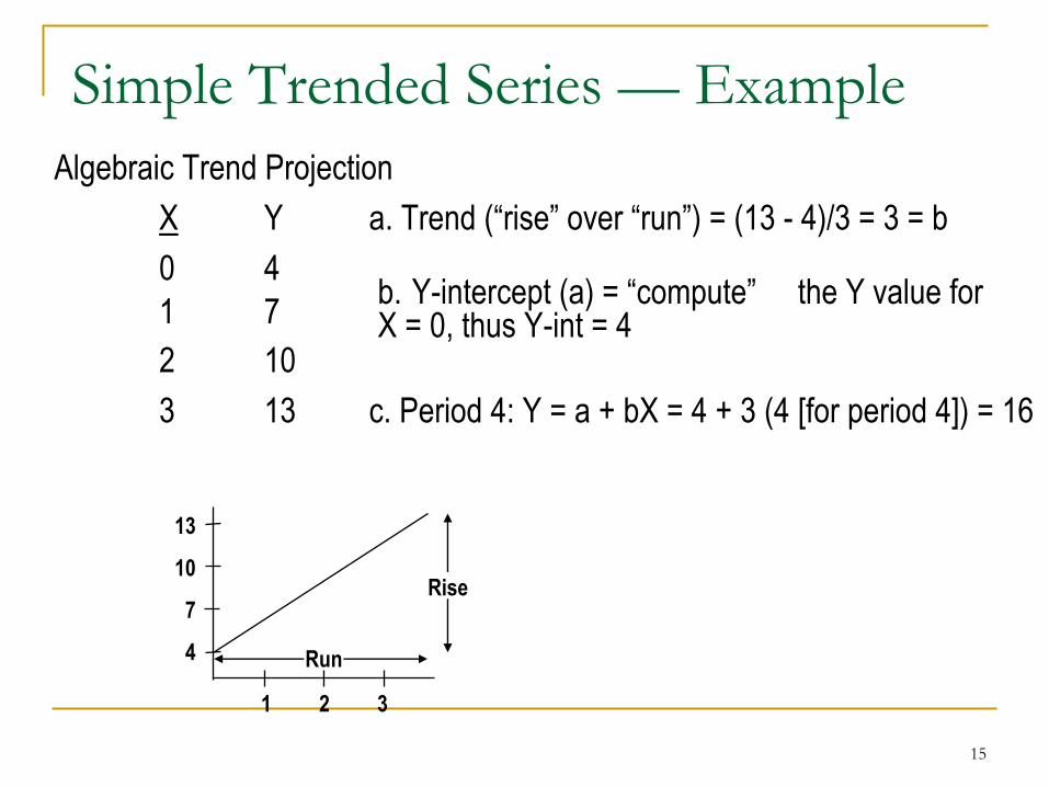
Simple Trended Series — ExampleAlgebraic Trend Projection
X Y a. Trend (“rise” over “run”) = (13 - 4)/3 = 3 = b 0 41 72 103 13 c. Period 4: Y = a + bX = 4 + 3 (4 [for period 4]) = 16
b. Y-intercept (a) = “compute” the Y value for X = 0, thus Y-int = 4
1 2 3
13
10
7
4 Run
Rise

16
Seasonal Series Indexing Sample Data
0 yr 1 yr 2 Seasonal
SeasonalMonth Year 1 Year 2 Year 3 Total Index
Jan 10 12 11 33 0.33Feb 13 13 11 37 0.37Mar 33 38 29 100 1.00
Apr 45 54 47 146 1.46May 53 56 55 164 1.64Jun 57 56 55 168 1.68
Jul 33 27 34 94 0.94Aug 20 18 19 57 0.57Sep 19 22 20 61 0.61
Oct 18 18 15 51 0.51Nov 46 50 45 141 1.41Dec 48 53 47 148 1.48
Total 395 417 388 1200 12.00
17
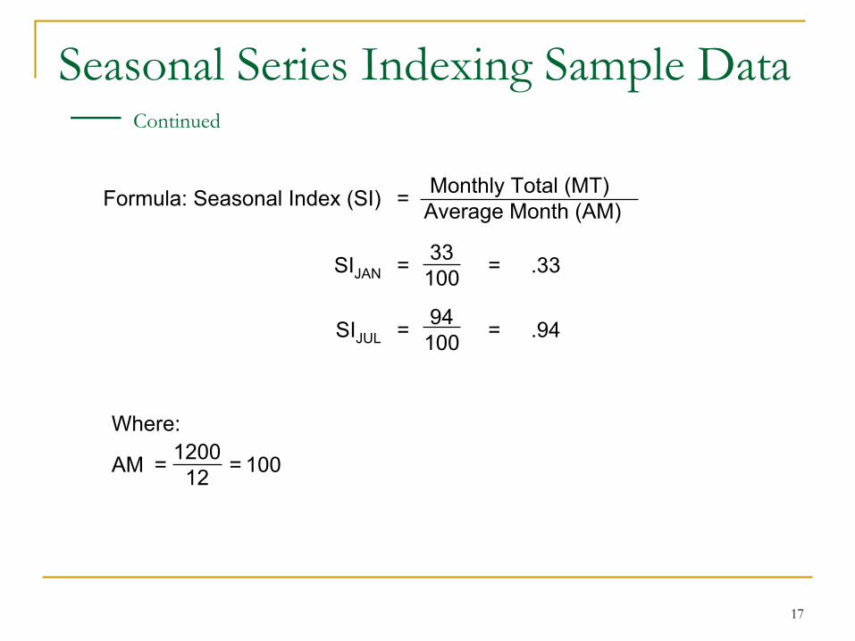
Seasonal Series Indexing Sample Data— Continued
Monthly Total (MT)Formula: Seasonal Index (SI) = Average Month (AM)
33SIJAN = = .33100
94SIJUL = = .94100
Where:1200AM = = 10012

18
è GivenDeseasonalized Seasonal
Demand Forecast IndexJuly 34 36 0.94Aug 0.57
1. Deseasonalize current (July) actual demand
2. Use exponential smoothing to project deseasonalized data oneperiod ahead (α = .2)
3. Reseasonalize forecast for desired month (August)= Deseasonalized forecast × seasonal factor = 36.03 × 0.57 = 20.53 or 21
36.03(36)(0.8)(36.17)(0.2))F(1DF TT1T =+=−+=+ αα
Forecast with Seasonal Indexes and Exponential Smoothing
34Actual demand Seasonal index 0.9436.17= =

19
Standard Deviation (sigma)F=
A =Actual
Error(Sales – Error
Period Forecast Sales Forecast) Squared1 1,000 1,200 200 40,0002 1,000 1,000 0 03 1,000 800 – 200 40,0004 1,000 900 – 100 10,0005 1,000 1,400 400 160,0006 1,000 1,200 200 40,0007 1,000 1,100 100 10,0008 1,000 700 – 300 90,0009 1,000 1,000 0 0
10 1,000 900 – 100 10,00010,000 10,200 200 400,000

20
Standard Deviation — Continued
Standard Deviation
20010
400,000
2119
400,000
==
==
ΝΟΤΕ: About the use of n or n - 1 in the above equations
n Use with a large population (> 30 observations)n - 1 Use with a small population (< 30 observations)
Standard Deviation
( )2
1i iA Fn
−−
∑
( )2i iA Fn−∑
21
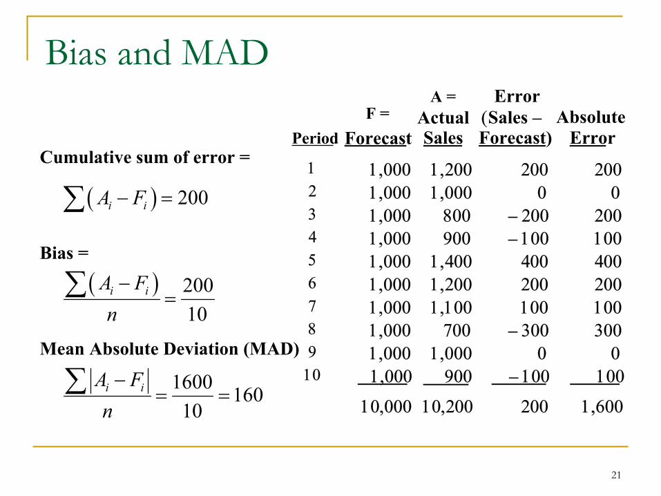
Cumulative sum of error =
Bias =
Mean Absolute Deviation (MAD)
Bias and MADF =
A =Actual
Error(Sales – Absolute
Period Forecast Sales Forecast) Error1 1,000 1,200 200 2002 1,000 1,000 0 03 1,000 800 – 200 2004 1,000 900 – 100 1005 1,000 1,400 400 4006 1,000 1,200 200 2007 1,000 1,100 100 1008 1,000 700 – 300 3009 1,000 1,000 0 010 1,000 900 – 100 100
10,000 10,200 200 1,600
( ) 200i iA F− =∑
( ) 20010
i iA Fn
−=∑
1600 16010
i iA Fn
−= =∑

22
Cumulative Sum of Error
Bias
Mean Absolute Deviation (MAD)
Standard Deviation
Measures of Forecast Error
ΝΟΤΕ: About the use of n or n - 1 in the above equations
n Use with a large population (> 30 observations)n - 1 Use with a small population (< 30 observations)
( )2
1i iA Fn
−−
∑
( )i iA F−∑( )i iA Fn
−∑
i iA Fn
−∑
( )2i iA Fn−∑or

23
Definition A confidence interval is a measure of distance, increments of which are represented by the z valueFormulas
Relationship
1 standard deviation (σ) = 1.25 × MAD
In the example data σ = 1.25 × 160 = 200
Confidence Intervals
s (1 Standard Deviation)
Source: Raz and Roberts, “Statistics,” 1987
( )2
1i iA Fn
−=
−∑ ( )2
i iA Fn−∑
Distance-MeanStandard Deviatiom
x xzs−
= =
or
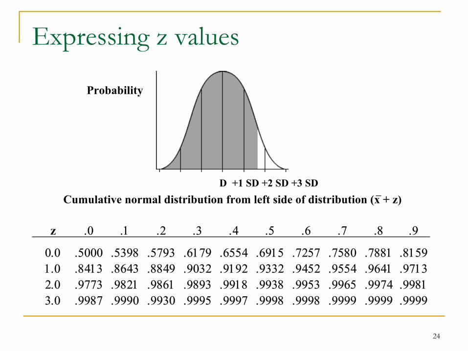
24
Expressing z values
Probability
D +1 SD +2 SD +3 SDCumulative normal distribution from left side of distribution (x + z)
z .0 .1 .2 .3 .4 .5 .6 .7 .8 .9
0.0 .5000 .5398 .5793 .6179 .6554 .6915 .7257 .7580 .78811.0 .8413 .8643 .8849 .9032 .9192 .9332 .9452 .9554 .96412.0 .9773 .9821 .9861 .9893 .9918 .9938 .9953 .9965 .99743.0 .9987 .9990 .9930 .9995 .9997 .9998 .9998 .9999 .9999
.8159
.9713
.9981
.9999
25
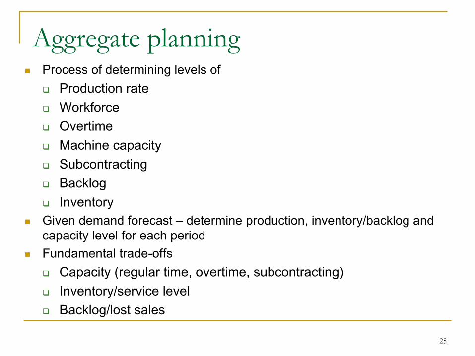
Aggregate planningProcess of determining levels of
Production rateWorkforce OvertimeMachine capacitySubcontractingBacklogInventory
Given demand forecast – determine production, inventory/backlog and capacity level for each periodFundamental trade-offs
Capacity (regular time, overtime, subcontracting)Inventory/service levelBacklog/lost sales

26
Aggregate planning strategiesStrategies - synchronizing production with demand
Chase- using capacity as the leverBY VARYING MACHINE OR WORKFORCE (numbers or flexibility)Difficult to implement and expensive. Low levels of inventory
Time flexibility – utilization as the leverIF EXCESS MACHINE CAPACITY, VARYING HOURS WORKED (workforce stable, hours vary)Low inventory and lower utilisation than chaseUseful when inventory cost high and capacity cheap
Level – using inventory as the leverStable workforce and capacityLarge inventories and backlogsMost practical and popular
27
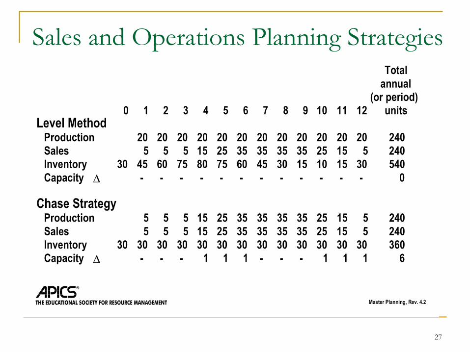
Sales and Operations Planning Strategies
Master Planning, Rev. 4.2
Totalannual
(or period)0 1 2 3 4 5 6 7 8 9 10 11 12 units
Level MethodProduction 20 20 20 20 20 20 20 20 20 20 20 20 240Sales 5 5 5 15 25 35 35 35 35 25 15 5 240Inventory 30 45 60 75 80 75 60 45 30 15 10 15 30 540Capacity ∆ - - - - - - - - - - - - 0
Chase StrategyProduction 5 5 5 15 25 35 35 35 35 25 15 5 240Sales 5 5 5 15 25 35 35 35 35 25 15 5 240Inventory 30 30 30 30 30 30 30 30 30 30 30 30 30 360Capacity ∆ - - - 1 1 1 - - - 1 1 1 6
28
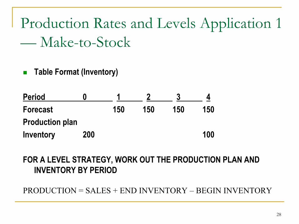
Production Rates and Levels Application 1 — Make-to-Stock
Table Format (Inventory)
Period 0 1 2 3 4Forecast 150 150 150 150Production planInventory 200 100
FOR A LEVEL STRATEGY, WORK OUT THE PRODUCTION PLAN AND INVENTORY BY PERIOD
PRODUCTION = SALES + END INVENTORY – BEGIN INVENTORY
29
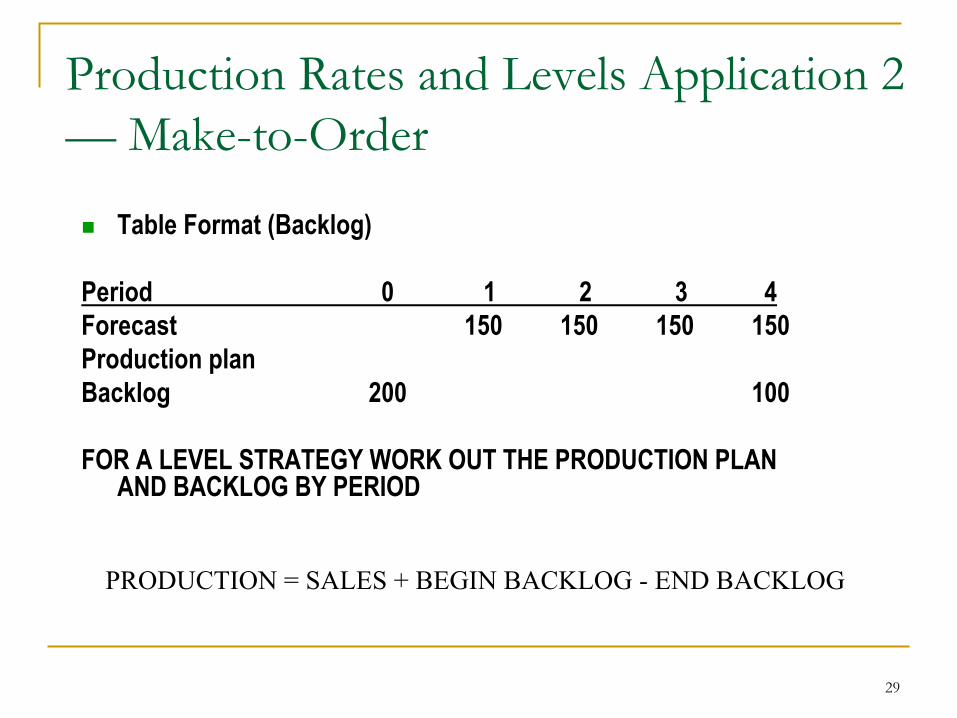
Production Rates and Levels Application 2 — Make-to-Order
Table Format (Backlog)
Period 0 1 2 3 4Forecast 150 150 150 150Production planBacklog 200 100
FOR A LEVEL STRATEGY WORK OUT THE PRODUCTION PLAN AND BACKLOG BY PERIOD
PRODUCTION = SALES + BEGIN BACKLOG - END BACKLOG
30
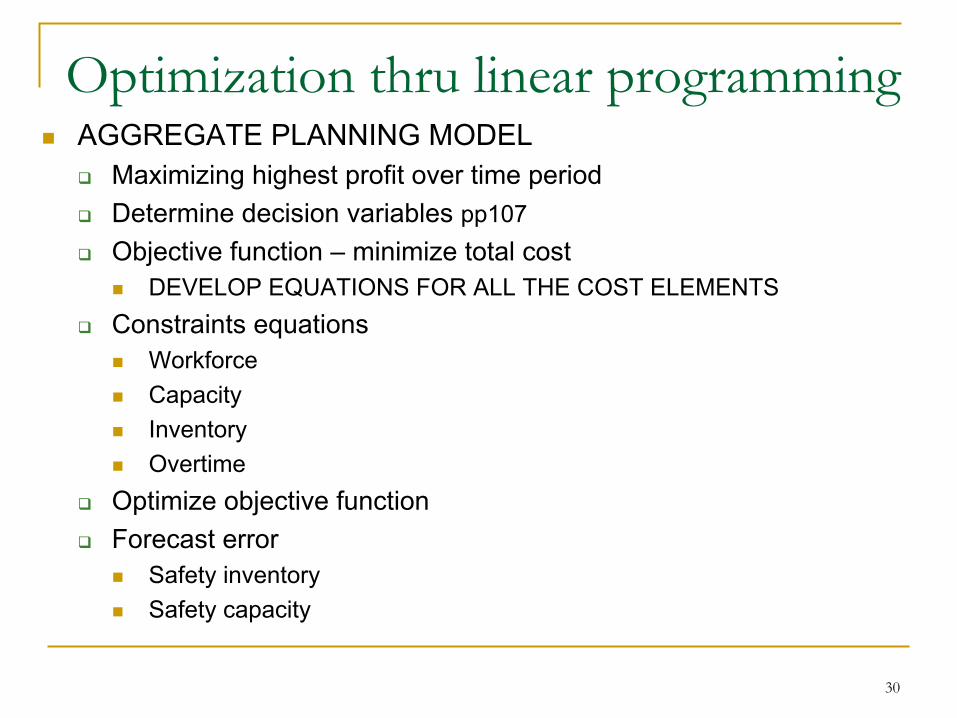
Optimization thru linear programmingAGGREGATE PLANNING MODEL
Maximizing highest profit over time periodDetermine decision variables pp107Objective function – minimize total cost
DEVELOP EQUATIONS FOR ALL THE COST ELEMENTSConstraints equations
WorkforceCapacityInventoryOvertime
Optimize objective functionForecast error
Safety inventorySafety capacity
31
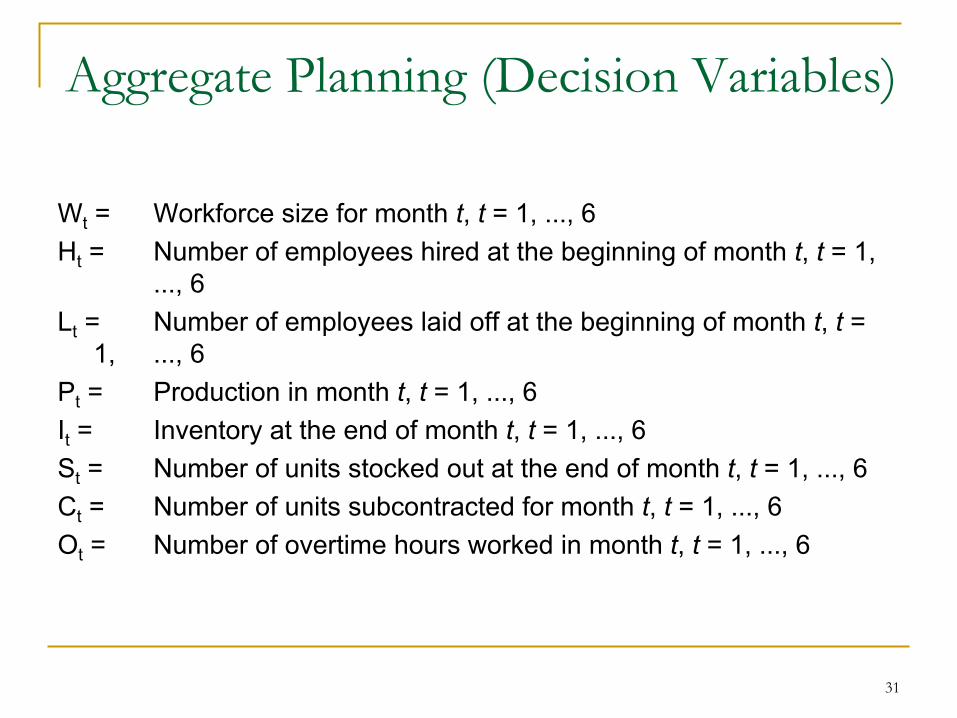
Aggregate Planning (Decision Variables)
Wt = Workforce size for month t, t = 1, ..., 6Ht = Number of employees hired at the beginning of month t, t = 1,
..., 6Lt = Number of employees laid off at the beginning of month t, t =
1, ..., 6Pt = Production in month t, t = 1, ..., 6It = Inventory at the end of month t, t = 1, ..., 6St = Number of units stocked out at the end of month t, t = 1, ..., 6Ct = Number of units subcontracted for month t, t = 1, ..., 6Ot = Number of overtime hours worked in month t, t = 1, ..., 6
32
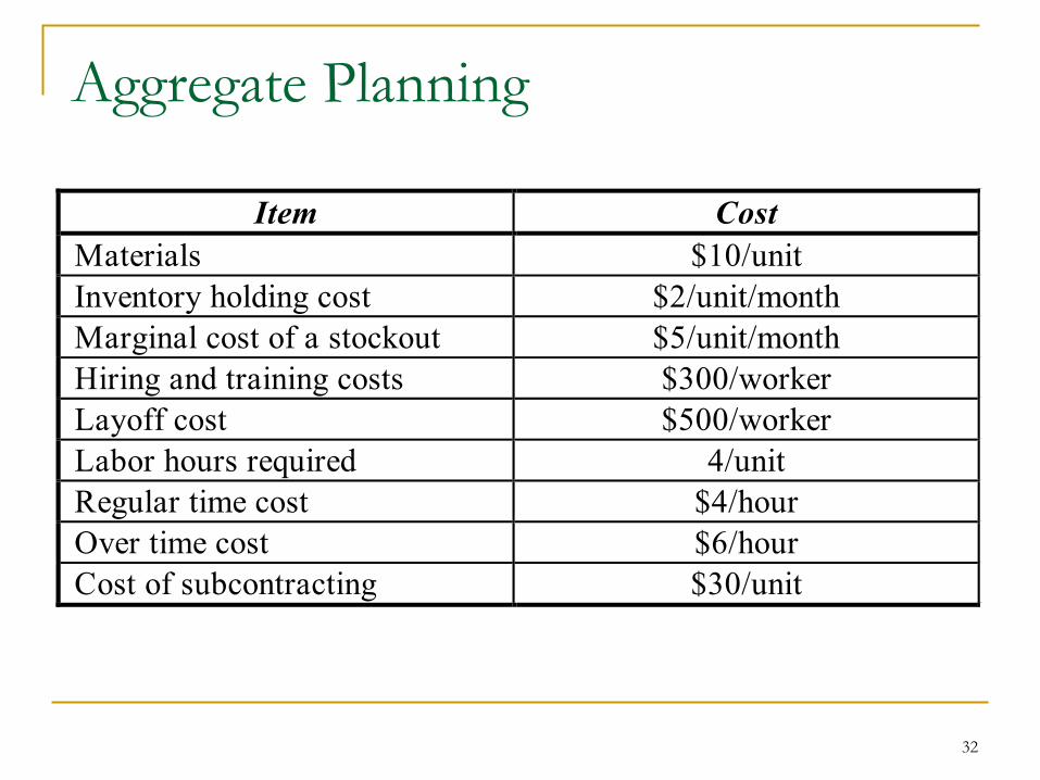
Aggregate Planning
Item CostMaterials $10/unitInventory holding cost $2/unit/monthMarginal cost of a stockout $5/unit/monthHiring and training costs $300/workerLayoff cost $500/workerLabor hours required 4/unitRegular time cost $4/hourOver time cost $6/hourCost of subcontracting $30/unit
33
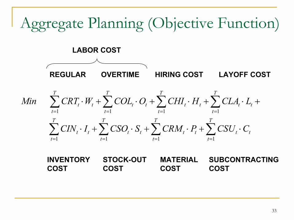
Aggregate Planning (Objective Function)
1 1 1 1
1 1 1 1
T T T T
t t t t t t t tt t t tT T T T
t t t t t t t tt t t t
Min CRT W COL O CHI H CLA L
CIN I CSO S CRM P CSU C
= = = =
= = = =
⋅ + ⋅ + ⋅ + ⋅ +
⋅ + ⋅ + ⋅ + ⋅
∑ ∑ ∑ ∑
∑ ∑ ∑ ∑
LABOR COST
HIRING COST LAYOFF COST
INVENTORY COST
STOCK-OUTCOST
MATERIALCOST
SUBCONTRACTINGCOST
REGULAR OVERTIME
34
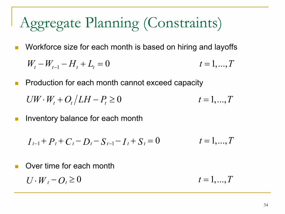
Aggregate Planning (Constraints)Workforce size for each month is based on hiring and layoffs
1 0 1,...,t t t tW W H L t T−− − + = =
0 1,...,t t tUW W O LH P t T⋅ + − ≥ =
Production for each month cannot exceed capacity
1 1 0 1,...,t t t tt t t t TC S SI P D I− −+ + − − − + = =
Inventory balance for each month
Over time for each month
0 1,...,t t t TU W O− ≥ =⋅
35
Aggregate planning in practice
Make plans flexible because forecasts are always wrong
Perform sensitivity analysis on the inputs – I.E. Look at effects of high/low
Rerun the aggregate plan as new data emergesUse aggregate planning as capacity utilization increases
When utilization is high, there is likely to be capacity limitations and all the orders will not be produced

36
Managing supply and demandpredictable variabilityPredictable variability – change in demand can be forecast
MANAGING DEMAND – short time price discounts, trade promotionsMANAGING SUPPLY – capacity, inventory, subcontracting & backlog, purchased product
Managing capacityTime flexibility from workforce (overtime)Use of seasonal workforceUse of subcontractingUse of dual facilities – dedicated and flexibleDesign product flexibility into productionUse of multi-purpose machines (cnc machine centers)
Managing inventoryUsing common components across multiple productsBuild inventory of high demand or predictable demand
37
Supplier partnershipsQualification and selection
Rationalization of supplier basePartnership
Win-win and trustSharing of risk and commitmentPrice reductions and increases based on forecastRate replenishment
Measurement and feedbackQuality, delivery, responsivenessQuarterly feedback Implications

38
Managing demand (predictable variability)
Manage demand with pricingFactors influencing the timing of a promotion:
Impact on demand; product margins; cost of holding inventory; cost of changing capacity
Demand increase (from discounting) due to:Market growthStealing market shareForward buying
Discount of $1 increases period demand by 10% and moves 20% of next two months demand forward
Reduce price by $1in Jan or April, increase sales by 10%

39
Process Flow Measures
FLOW RATE (Rt), CYCLE TIME (Tt), & INVENTORY (It) RELATIONSHIPS
F = Flow Rate or Throughput is output of a line in pieces per timeT = Cycle time is the time taken to complete an operationI = Inventory is the material on the lineLITTLE’s LAW:
Av. I = Av. R x Av. T x Variability factor Examples:
If Inventory is 100 pieces and Cycle time is 10 hours, the Throughput rate is 10 pcs per hourIf Cycle time is halved; Throughput is doubledIf Inventory is halved; cycle time is halved
40
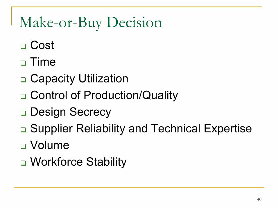
Make-or-Buy DecisionCostTimeCapacity UtilizationControl of Production/QualityDesign SecrecySupplier Reliability and Technical ExpertiseVolumeWorkforce Stability
41
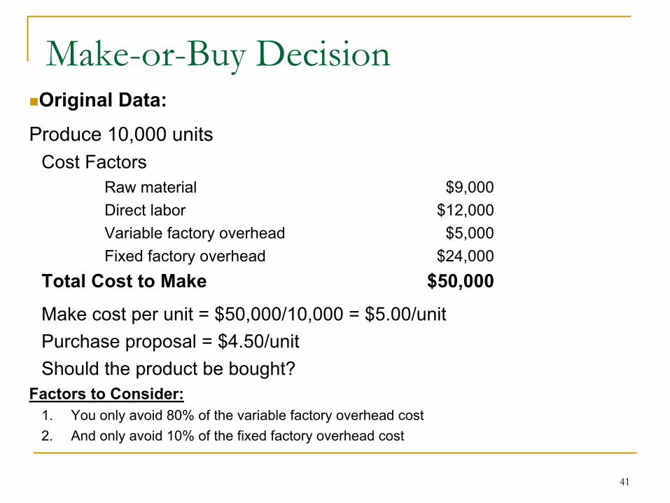
Make-or-Buy DecisionOriginal Data:
Produce 10,000 unitsCost Factors
Raw material $9,000Direct labor $12,000Variable factory overhead $5,000Fixed factory overhead $24,000
Total Cost to Make $50,000
Make cost per unit = $50,000/10,000 = $5.00/unitPurchase proposal = $4.50/unitShould the product be bought?
Factors to Consider:1. You only avoid 80% of the variable factory overhead cost2. And only avoid 10% of the fixed factory overhead cost

42
Cost Avoidance Analysis (Solution)Solution
Cost avoided by purchasingTotal cost to make $50,000
Less cost avoided:Raw material $9,000Direct labor $12,000Variable factory overhead ($5,[email protected]) $4,000Fixed factory overhead ($24,[email protected]) $2,400
Total Avoided Cost $27,400Analysis
Cost not avoided $22,600Plus cost to purchase $45,000Total cost to purchase $67,600
Compare to cost to make $50,000Increase in cost to purchase $17,600Actual cost per purchased item 67500/1000 = $6.75/unit !
43
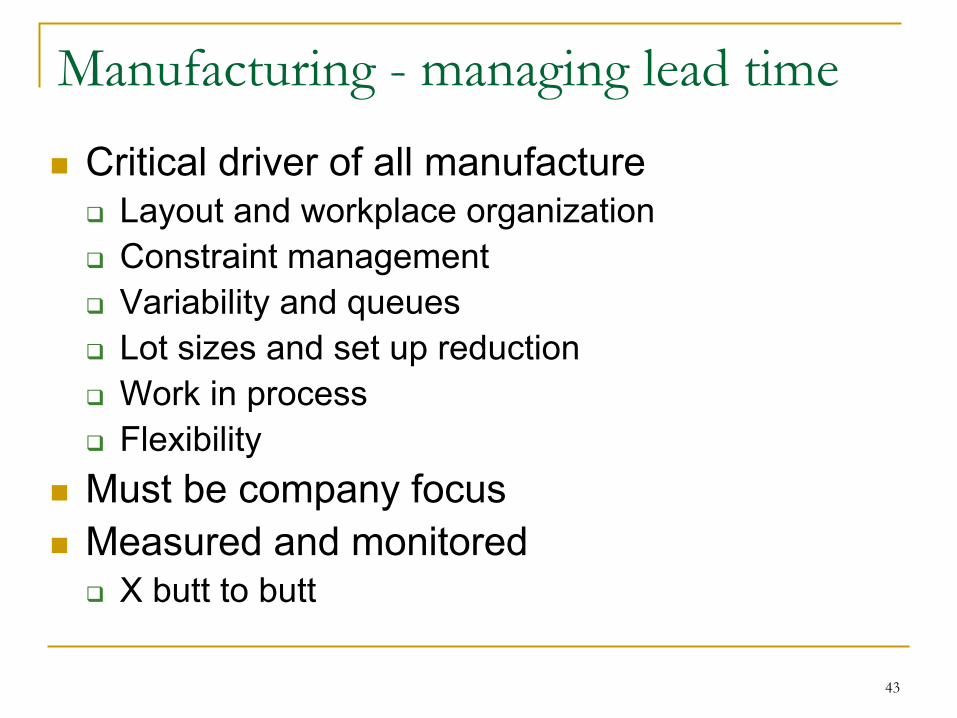
Manufacturing - managing lead timeCritical driver of all manufacture
Layout and workplace organizationConstraint managementVariability and queuesLot sizes and set up reductionWork in processFlexibility
Must be company focusMeasured and monitored
X butt to butt
44
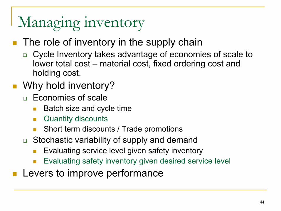
Managing inventoryThe role of inventory in the supply chain
Cycle Inventory takes advantage of economies of scale to lower total cost – material cost, fixed ordering cost and holding cost.
Why hold inventory?Economies of scale
Batch size and cycle timeQuantity discountsShort term discounts / Trade promotions
Stochastic variability of supply and demandEvaluating service level given safety inventoryEvaluating safety inventory given desired service level
Levers to improve performance
45
Predictable variability in practiceCoordinate marketing, sales and operations
Sales and operations planningOne goal maximizing profit, one game plan
Take predicable variability into account when making strategic decisionsPartner with principal customers, eliminate predictions!Preempt (promos etc.). Do not just react to predictable variability


![ifac - Carnegie Mellon Universitycepac.cheme.cmu.edu/pasilectures/crisalle/[WiAA] Computer... · 2005. 7. 29. · Title: ifac.dvi Created Date: 191020613161130](https://static.documents.pub/doc/80x56/60aab919e49cba3c54281da2/ifac-carnegie-mellon-wiaa-computer-2005-7-29-title-ifacdvi-created.jpg)