

NBER WORKING PAPER SERIES
VOLATILITY, LABOR MARKET FLEXIBILITY, AND THE PATTERN OF COMPARATIVEADVANTAGE
Alejandro CuñatMarc J. Melitz
Working Paper 13062http://www.nber.org/papers/w13062
NATIONAL BUREAU OF ECONOMIC RESEARCH1050 Massachusetts Avenue
Cambridge, MA 02138April 2007
We are grateful to Pol Antràs, Gordon Hanson, Peter Neary, Barbara Petrongolo, Steve Redding, TonyVenables, Jaume Ventura, and seminar participants in Alicante, Banco de España, Bocconi, Cambridge,ERWIT 2006, Harvard, LSE, NBER, Oxford, Pompeu Fabra, Princeton, Valencia, the AEA 2006 Meeting,and the EEA 2006 Meeting for helpful discussions and suggestions. Kalina Manova, Martin Stewart,and Rob Varady provided superb research assistance. All errors remain ours. Cuñat gratefully acknowledgesfinancial support from CICYT (SEC 2002-0026). Melitz thanks the International Economics Sectionat Princeton University for its hospitality while this paper was written. The views expressed hereinare those of the author(s) and do not necessarily reflect the views of the National Bureau of EconomicResearch.
© 2007 by Alejandro Cuñat and Marc J. Melitz. All rights reserved. Short sections of text, not to exceedtwo paragraphs, may be quoted without explicit permission provided that full credit, including © notice,is given to the source.

Volatility, Labor Market Flexibility, and the Pattern of Comparative AdvantageAlejandro Cuñat and Marc J. MelitzNBER Working Paper No. 13062April 2007JEL No. F1,F16
ABSTRACT
This paper studies the link between volatility, labor market flexibility, and international trade. Internationaldifferences in labor market regulations affect how firms can adjust to idiosyncratic shocks. These institutionaldifferences interact with sector specific differences in volatility (the variance of the firm-specific shocksin a sector) to generate a new source of comparative advantage. Other things equal, countries withmore flexible labor markets specialize in sectors with higher volatility. Empirical evidence for a largesample of countries strongly supports this theory: the exports of countries with more flexible labormarkets are biased towards high-volatility sectors. We show how differences in labor market institutionscan be parsimoniously integrated into the workhorse model of Ricardian comparative advantage ofDornbusch, Fischer, and Samuelson (1977). We also show how our model can be extended to multiplefactors of production.
Alejandro CuñatUniversity of EssexWivenhoe ParkColchester CO4 3SQUnited Kingdomand CEP and CEPR [email protected]
Marc J. MelitzDept of Economics & Woodrow Wilson SchoolPrinceton University308 Fisher HallPrinceton, NJ 08544and CEPR and [email protected]
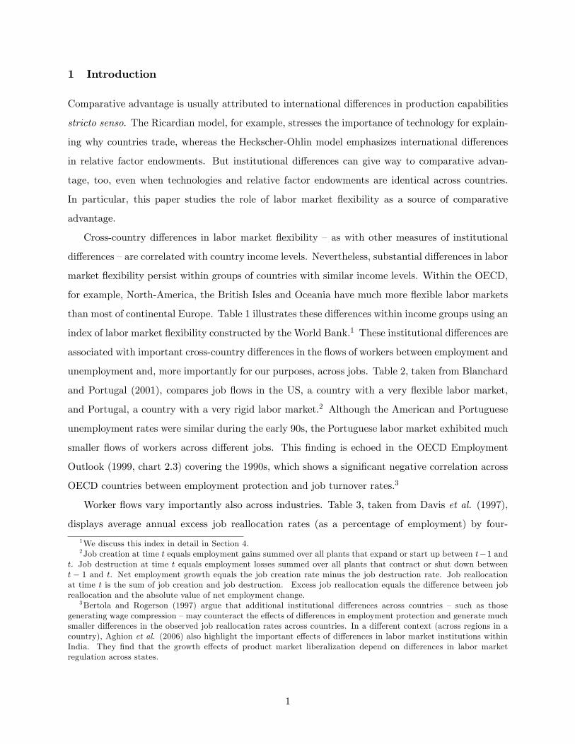
1 Introduction
Comparative advantage is usually attributed to international di¤erences in production capabilities
stricto senso. The Ricardian model, for example, stresses the importance of technology for explain-
ing why countries trade, whereas the Heckscher-Ohlin model emphasizes international di¤erences
in relative factor endowments. But institutional di¤erences can give way to comparative advan-
tage, too, even when technologies and relative factor endowments are identical across countries.
In particular, this paper studies the role of labor market �exibility as a source of comparative
advantage.
Cross-country di¤erences in labor market �exibility �as with other measures of institutional
di¤erences �are correlated with country income levels. Nevertheless, substantial di¤erences in labor
market �exibility persist within groups of countries with similar income levels. Within the OECD,
for example, North-America, the British Isles and Oceania have much more �exible labor markets
than most of continental Europe. Table 1 illustrates these di¤erences within income groups using an
index of labor market �exibility constructed by the World Bank.1 These institutional di¤erences are
associated with important cross-country di¤erences in the �ows of workers between employment and
unemployment and, more importantly for our purposes, across jobs. Table 2, taken from Blanchard
and Portugal (2001), compares job �ows in the US, a country with a very �exible labor market,
and Portugal, a country with a very rigid labor market.2 Although the American and Portuguese
unemployment rates were similar during the early 90s, the Portuguese labor market exhibited much
smaller �ows of workers across di¤erent jobs. This �nding is echoed in the OECD Employment
Outlook (1999, chart 2.3) covering the 1990s, which shows a signi�cant negative correlation across
OECD countries between employment protection and job turnover rates.3
Worker �ows vary importantly also across industries. Table 3, taken from Davis et al. (1997),
displays average annual excess job reallocation rates (as a percentage of employment) by four-
1We discuss this index in detail in Section 4.2Job creation at time t equals employment gains summed over all plants that expand or start up between t�1 and
t. Job destruction at time t equals employment losses summed over all plants that contract or shut down betweent � 1 and t. Net employment growth equals the job creation rate minus the job destruction rate. Job reallocationat time t is the sum of job creation and job destruction. Excess job reallocation equals the di¤erence between jobreallocation and the absolute value of net employment change.
3Bertola and Rogerson (1997) argue that additional institutional di¤erences across countries � such as thosegenerating wage compression �may counteract the e¤ects of di¤erences in employment protection and generate muchsmaller di¤erences in the observed job reallocation rates across countries. In a di¤erent context (across regions in acountry), Aghion et al. (2006) also highlight the important e¤ects of di¤erences in labor market institutions withinIndia. They �nd that the growth e¤ects of product market liberalization depend on di¤erences in labor marketregulation across states.
1

digit (US SIC) manufacturing industry in the US. Excess job reallocation re�ects simultaneous job
creation and destruction within industries. It represents the �excess�portion of job reallocation �
over and above the amount required to accommodate net industry employment changes. Table 3
shows that the within-industry reallocation process exhibits a remarkable degree of cross-industry
variation. Clearly, this variation cannot be attributed to di¤erences in labor market regulation.
We interpret this cross-industry variation as re�ecting di¤erences in the needed adjustments, at the
�rm-level, to idiosyncratic demand and productivity shocks: a higher within-industry dispersion of
shocks entails a larger response in the within-industry reallocation of employment between �rms.
We formalize a theory of comparative advantage in this context. For simplicity, we frame our
insights within a one-factor model of trade between two countries with di¤erent labor market insti-
tutions (a ��exible�and �rigid�economy). These di¤erences interact with industry-level di¤erences
in the dispersion of �rm-level shocks to generate industry-level di¤erences in relative productivity,
and hence a �Ricardian�source of comparative advantage. Again for simplicity, we do not model
any technological di¤erences between countries. Thus, in the absence of shocks, di¤erences in labor
market �exibility are irrelevant. There is then no source of comparative advantage, and no motive
for trade. However, in the presence of �rm-level shocks, the country with �exible labor markets can
reallocate labor across �rms more easily � leading to higher industry average productivity levels
relative to the country with rigid labor markets. This productivity di¤erence is then magni�ed by
the dispersion of the within-industry shocks, which we refer to as industry volatility. The latter
thus interacts with the institutional labor market di¤erences to induce a pattern of comparative
advantage across industries.
We also extend our model to incorporate a second factor, capital, whose reallocation across �rms
is not a¤ected by the labor market institutions. Provided that this reallocation of capital across
�rms is subject to the same degree of rigidity in both countries, then the pattern of comparative
advantage driven by industry volatility becomes more muted for capital intensive industries. In
other words, rigid countries face less of a comparative disadvantage in capital intensive industries
� holding industry volatility constant. Thus our model also explains how capital intensity can
a¤ect comparative advantage based on di¤erences in labor market institutions �separately from
the standard Hecksher-Ohlin e¤ect via interactions with a country�s capital abundance.
Besides these implications on comparative advantage, our model also yields interesting insights
on the relationship between trade and unemployment in countries that su¤er from important rigidi-
ties in their labor markets: trade with a �exible country imposes a trade-o¤ between the wage rate
2

(relative to that of the �exible economy) and its employment level. As the rigid economy�s rel-
ative wage rises, foreign competition shrinks the range of sectors with a comparative advantage,
and labor demand falls. This trade-o¤ worsens with increases in labor market rigidity and with
across-the-board (cross-industry) increases in volatility, as both of these phenomena enhance the
�exible economy�s competitiveness relative to the rigid economy.
We then empirically test the predictions of our model on the observed pattern of comparative
advantage for a large sample of countries, using country-level export data at a detailed level of
sector disaggregation (hundreds of sectors).4 We thus test whether countries with relatively more
�exible labor markets concentrate their exports relatively more intensively in sectors with higher
volatility. We also test the additional prediction of our model that capital intensity reduces this
e¤ect of volatility for countries with relatively more rigid labor markets. Naturally, we also control
for other determinants of comparative advantage such as the interactions between country-level
factor abundance and sector-level factor intensities. We use two distinct estimation approaches
towards these goals. The �rst approach, in the spirit of Romalis (2004), uses the full cross-section
of commodity exports across countries and sectors to test for interaction e¤ects between the country-
level and sector-level characteristics that jointly determine comparative advantage.5 Recognizing
some important limitations (both theoretical and empirical) associated with this method, we also
use a second more robust approach based on a country-level analysis. Both approaches strongly
con�rm our theoretical results.
The potential links between labor markets and comparative advantage have received an increas-
ing level of attention in the recent trade literature. Saint-Paul (1997) analyzes the links between
�ring costs and international specialization according to the life-cycle of goods: countries with
�exible labor markets exhibit a comparative advantage in �new�industries subject to higher aggre-
gate demand volatility (relative to more �mature�industries). Haaland and Wooton (forthcoming)
also focus on di¤erences in �ring costs across countries, and examine their implications for the
location of multinational a¢ liates. Davidson et al. (1999) present an equilibrium unemployment
model in which the country with a more e¢ cient search technology has a comparative advantage
in the good produced in high-unemployment/high-vacancy sectors. This is due to the di¤erences
in prices required to induce factors to search for matches in sectors with di¤erent break-up rates.
Galdón (2002) shows that labor market rigidities can also a¤ect specialization through long-term
4Data on value added by industry, such as UNIDO, provide much less �ner levels of disaggregation.5There is also a substantial earlier literature, starting with the work of Baldwin (1971, 1979), that examined the
relationship between the structure of commodity exports and patterns of factor abundance.
3

unemployment, which reduces the skills workers may need in �new-economy�sectors. In the current
paper, we focus on a relatively more tractable theoretical framework that lends itself to more direct
empirical testing. In particular, we highlight the role of �rm-level volatility, which can be measured
across sectors, in shaping the pattern of comparative advantage.6
Our paper is also related to a growing literature that studies the e¤ects of international dif-
ferences in institutions on trade patterns. Levchenko (2004) shows that the quality of institutions
(e.g., property rights, the quality of contract enforcement, shareholder protection) a¤ects both trade
�ows and the distribution of the gains from trade between rich and poor countries. Costinot (2005)
and Nunn (2005) extend models of trade with imperfect contracts, highlighting a link between
country institutions (linked to contract enforcement) and the pattern of comparative advantage
across sectors with di¤erent technological characteristics (which a¤ect the sector�s reliance on con-
tract enforcement, such as the complexity of production or the need for relation-speci�c investments
by workers). Finally, our work is also related to a number of papers that study the relationship
between international trade and labor market outcomes in the presence of labor market rigidities.
See, among others, the classic contributions by Brecher (1974a, 1974b), followed by the more recent
contributions of Matusz (1996), Davis (1998a, 1998b), and Brügemann (2003).
The rest of the paper is structured as follows. Section 2 formalizes the paper�s basic insights
in a one-factor model. Section 3 extends the model�s implications for comparative advantage to a
two-factor setup. In section 4, we present the empirical evidence. Section 5 concludes. An appendix
discusses some analytical details.
2 The Model
There are two countries, denoted by c = F;H. Each country is endowed with �L units of labor,
which are supplied inelastically (for any positive wage) and internationally immobile. Preferences
are identical across countries. Agents maximize utility over a Cobb-Douglas aggregate Q of a
continuum of �nal goods q(i); indexed by i:
Q � exp�Z 1
0ln q (i) di
�:
6Koren and Tenreyro (2005) and di Giovanni and Levchenko (2006) also study the relationship between industryvolatility and specialization, but do not relate it to international di¤erences in labor market institutions.
4

In each industry i; the �nal good is produced using a continuum of intermediate goods y(i; z)
according to the technology
y (i) =
�Z 1
0y (i; z)
"�1" dz
� ""�1
; (1)
where y (i) denotes production of the �nal good i. We assume that these intermediate goods are
gross substitutes: " > 1 (and thus that the intermediate goods used to produce a given �nal good
are less di¤erentiated than the �nal goods across industries). Each intermediate good is produced
with labor only:
y (i; z) = e�L (i; z) ;
where � is a stochastic term. Within each industry, the �0s are iid draws from a common distribution
Gi(:), identical across countries, but di¤erent across industries, with mean 0 and variance �2 (i).
We refer to �2 (i) as industry i�s �volatility�. This formulation emphasizes shocks to intermediate
good producers on the production side, but is nonetheless isomorphic to a formulation emphasizing
demand shocks in equation (1). As a given realization of the productivity draw � uniquely identi�es
an intermediate good producer z, we now switch to the use of this draw � as our index for the
intermediate goods.
We assume two di¤erent institutional scenarios. In country F , all markets are competitive, and
the determination of all prices and the allocation of all resources take place after the realization of
�. This captures the idea of a �exible economy that can costlessly reallocate resources towards their
more e¢ cient use. In countryH, a wage is negotiated (e.g., by a labor union) and intermediate good
producers then hire workers before the realization of �; no labor adjustment is allowed thereafter.
This corresponds to the idea that rigidities prevent �rms from adjusting to changing circumstances.
We assume that the unemployed, if any, cannot bid down the economy-wide ex-ante speci�ed wage,
and that the intermediate good producer is contractually committed to paying the hired number
of workers the negotiated wage (regardless of the realization of �). After the realization of �,
production and commodity market clearing take place in a competitive setting, subject to the wage
and employment restrictions. Intermediate goods producers anticipate this equilibrium, and adjust
their contracted labor demand accordingly. Given ex-ante free entry into the intermediate goods
sector, expected pro�ts of the intermediate good producers are driven to zero.
Throughout the paper, we do not explicitly model the potential bene�ts derived from employ-
ment stability nor the determination of the negotiated wage. We assume that the level of labor
market rigidity is pre-determined at the time the wage wH is chosen. We then model the poten-
5

tial repercussions for aggregate employment LH , potentially leading to unemployment whenever
LH < �L (�exible wages ensure full employment in the �exible economy, LF = �L).7 We thus focus
our analysis on the repercussion of these choices for the pattern of comparative advantage. Al-
though the institutional di¤erences outlined above between the two countries are rather stark, we
show in the appendix how our entire analysis can be extended to two countries with varying degrees
of labor market �exibility. This degree of labor market �exibility can vary continuously between
the extremes of the �exible and rigid economy described above.
Autarky in the Flexible Country
The zero-pro�t conditions for �nal good and intermediate good producers imply, respectively:
pF (i) =
�Z 1
�1pF (i; �)
1�" dGi (�)
� 11�"
;
pF (i; �) = e��wF :
This yields
pF (i) =wFhR1
�1 e("�1)�dGi (�)i 1"�1
; (2)
where ~�F (i) �hR1�1 e("�1)�dGi (�)
i 1"�1
represents the productivity level in industry i. This is
a weighted average of the productivity levels of the intermediate good producers e�, where the
weights are proportional to the intermediate good�s cost share in the �nal good production. The
corresponding goods and factor market clearing conditions close the model.
Autarky in the Rigid Country
Notice that the law of large numbers ensures there is no aggregate uncertainty. This implies that
expectations on all variables before the realization of � equal their ex-post counterparts except
for, of course, the individual �rm�s realization. We assume that agents hold a diversi�ed portfolio
and that �rms maximize expected pro�ts. Given that all �rms in industry i are ex-ante identical,
7One can also think about the rigid economy without unemployment as an economy where institutions prohibit theenforcement of employment contracts contingent on the realization of the shock �. Following this re-interpretation,for both the �exible and rigid economy, employment contracts must be agreed upon before the realization of theshock �. The key di¤erence between the two economies is that such contracts in the �exible economy can be madecontingent upon the future realization of the shock. This setup obviates the need to appeal to any wage settinginstitution in the rigid economy. The equilibrium in the rigid economy is then the competitive outcome contingenton the contractual incompleteness.
6

LH (i; z) = LH (i) for all z. Ex-ante zero-pro�t conditions and market clearing imply:
pH (i) =
�Z 1
�1pH (i; �)
1�" dGi (�)
� 11�"
; (3)
wHLH (i) =
Z 1
�1pH (i; �) yH (i; �) dGi (�) ; (4)
e�LH (i) =
�pH (i; �)
pH (i)
��"yH (i) : (5)
Equation (3) sets the price of �nal good i equal to its unit cost; equation (4) equates the labor cost
of an intermediate good producer in industry i with expected revenue (hence ex-ante zero pro�ts
for those producers); equation (5) enforces market clearing for intermediate goods in industry i.8
These equations yield
pH (i) =wHhR1
�1 e("�1)"
�dGi (�)i ""�1
; (6)
where ~�H(i) �hR1�1 e
("�1)"
�dGi (�)i ""�1
represents the productivity level in industry i for the rigid
economy.
As with the productivity ~�F (i) in the �exible economy, this productivity is a weighted av-
erage of the productivity levels of the intermediate good producers. Although the distribution
of these intermediate good productivity levels are identical in both countries (for each sector i),
the productivity averages are di¤erent as the cost shares of the intermediate goods in �nal good
production systematically vary across countries. Final good producers in the �exible country can
take full advantage of the dispersion of productivity levels among intermediate good producers by
optimally shifting their expenditures towards the more productive ones (with lower prices). This
reallocation process is constrained by the labor market rigidities in the other country. This, in turn,
confers an absolute advantage to the �exible economy across all sectors: ~�F (i) � ~�H(i) 8i, where
this inequality is strict whenever Gi(�) is non-degenerate (and there are idiosyncratic productivity
shocks).9
8Despite the labor market rigidity, the labor market clears under autarky: the law of large numbers implieszero pro�ts at the industry level, pH (i) yH (i) = wHLH (i) 8i. The labor market clearing condition then yieldsR 10LH (i) di =
R 10
pH (i)yH (i)wH
di = LH , and holds for LH = �L. The choice of wH proportionally shifts all prices pH(i)and has no e¤ect on employment.
9This is a direct application of Jensen�s inequality.
7
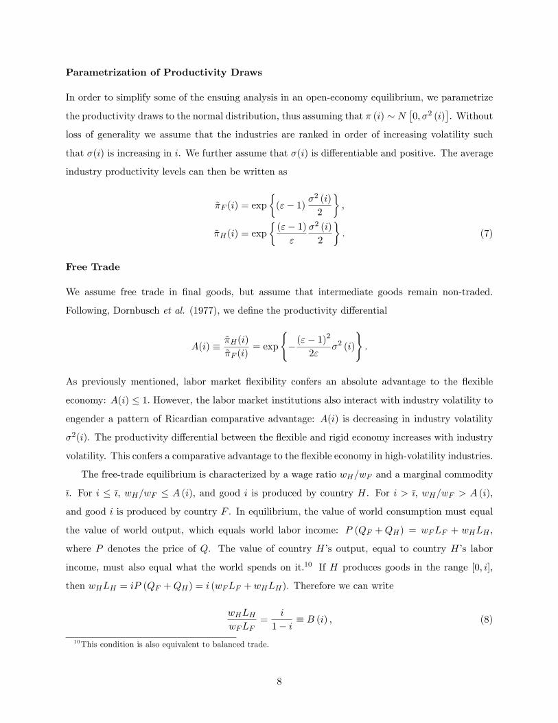
Parametrization of Productivity Draws
In order to simplify some of the ensuing analysis in an open-economy equilibrium, we parametrize
the productivity draws to the normal distribution, thus assuming that � (i) � N�0; �2 (i)
�. Without
loss of generality we assume that the industries are ranked in order of increasing volatility such
that �(i) is increasing in i. We further assume that �(i) is di¤erentiable and positive. The average
industry productivity levels can then be written as
~�F (i) = exp
�("� 1) �
2 (i)
2
�;
~�H(i) = exp
�("� 1)"
�2 (i)
2
�: (7)
Free Trade
We assume free trade in �nal goods, but assume that intermediate goods remain non-traded.
Following, Dornbusch et al. (1977), we de�ne the productivity di¤erential
A(i) � ~�H(i)
~�F (i)= exp
(�("� 1)
2
2"�2 (i)
):
As previously mentioned, labor market �exibility confers an absolute advantage to the �exible
economy: A(i) � 1: However, the labor market institutions also interact with industry volatility to
engender a pattern of Ricardian comparative advantage: A(i) is decreasing in industry volatility
�2(i). The productivity di¤erential between the �exible and rigid economy increases with industry
volatility. This confers a comparative advantage to the �exible economy in high-volatility industries.
The free-trade equilibrium is characterized by a wage ratio wH=wF and a marginal commodity
�{. For i � �{, wH=wF � A (i), and good i is produced by country H. For i > �{, wH=wF > A (i),
and good i is produced by country F . In equilibrium, the value of world consumption must equal
the value of world output, which equals world labor income: P (QF +QH) = wFLF + wHLH ,
where P denotes the price of Q. The value of country H�s output, equal to country H�s labor
income, must also equal what the world spends on it.10 If H produces goods in the range [0; i],
then wHLH = iP (QF +QH) = i (wFLF + wHLH). Therefore we can write
wHLHwFLF
=i
1� i � B (i) ; (8)
10This condition is also equivalent to balanced trade.
8

where B0(i) > 0. In closing the model, we distinguish between two cases, which depend on the
chosen level of wH relative to wF , and its consequences for unemployment in the rigid economy. We
normalize wF = 1, and thus emphasize that the chosen wage level wH in the rigid economy is an
indicator of worker purchasing power relative to the �exible economy. Recall that full employment
prevails in the �exible economy, ensuring that LF = �L is exogenously given.
Full Employment in the Rigid Country
We �rst assume that wH is chosen in order to generate full employment, hence LH = �L. In this case,
the intersection of A (i) and B (i) determines the free-trade equilibrium. (See Figure 1.) An overall
increase in volatility such that �0 (i) > � (i) ; 8i, causes A(i) to shift down while B(i) remains
unchanged. (See again Figure 1.) This leads to a decrease in the range of �nal goods produced in
H (i.e. a lower �{) and a lower relative wage wH . Such an overall increase in volatility (as has been
empirically measured in the last half century for the US) thus alters the pattern of comparative
advantage, inducing relative welfare gains for the economy with �exible labor markets.
Unemployment in the Rigid Country
We now assume that wH is chosen above its market-clearing level. Recall that countryF�s labor
market clears, so that LF = �L. In this case, the condition wH = A (�{) determines the equilibrium
specialization pattern: �{ = �{ (wH). Notice that, since A (�) is negatively sloped, @�{=@wH < 0.
Goods market clearing requires wHLH=�L = �{ (wH) = [1� �{ (wH)] = B (wH), where B (�) depends
negatively on wH . It is easy to see that country H�s employment level depends negatively on wH ,
too: LH = �LB (wH) =wH , @LH=@wH < 0. Hence, free trade with a �exible economy imposes a
trade-o¤ between the relative wage rate and unemployment in the rigid economy: as wH rises, the
range of sectors in which country H is competitive shrinks due to foreign competition, and labor
demand falls.
This implies that an increase in volatility across all industries will worsen the trade-o¤ be-
tween the relative wage wH and unemployment��L� LH
�. To see this more precisely, assume
that volatility can vary in all industries by a proportional factor > 0. That is, �0 (i) = � (i),
where �0 (i) denotes the new standard deviation of productivity shocks. In this case, wH = A (�{; ),
�{ = �{ (wH ; ), LH = �LB (wH ; ) =wH , @LH=@wH < 0, and @LH=@ < 0. An overall increase in
volatility thus leads to higher unemployment levels at a given relative wage wH , or to decreases
in the latter at a given employment level LH . In the appendix we allow for a continuous index
9

of labor market �exibility � in both countries, where a higher � represents a more �exible labor
market. We show that increases in �F � �H have e¤ects equivalent to those of an increase in �.
A word of caution is needed here. We stress that these comparative statics involve the relative
wage wH=wF , and not the real wage wH=P in the rigid economy. The standard gains from trade
also apply to this model, so that trade improves welfare in both countries, and hence the real wage
wH=P in the rigid economy. Overall increases in volatility also induce aggregate welfare gains as
they induce absolute increases in productivity levels. Our analysis emphasizes that these gains are
biased towards the �exible economy, improving relative welfare therein.
3 Two Factors
We now develop a two-factor version of our model.11 We assume that countries are endowed with
both capital and labor, and that industries di¤er in terms of capital intensity as well as volatility.
The Cobb-Douglas aggregate good Q is now de�ned according to
Q � exp�Z 1
0
Z 1
0ln q (i; j) didj
�;
where an industry is now characterized by a pair (i; j) representing an index for both volatility (i)
and capital intensity (j). The �nal good in each industry is still produced from a C.E.S. continuum
of intermediate goods indexed by z:
y (i; j) =
�Z 1
0y (i; j; z)
"�1" dz
� ""�1
;
Intermediate goods are now produced with both capital and labor, according to
y (i; j; z) = e��K(i; j; z)
� (j)
��(j) �L(i; j; z)1� � (j)
�1��(j); (9)
where � (j) 2 [0; 1] is the industry�s cost share of capital and the index of capital intensity. As in
the one-factor model, the �0s are iid draws from a common distribution, identical across countries,
but di¤erent across industries. We maintain the Normal parametrization for the productivity draws
� (i) � N�0; �2 (i)
�. Labor market �exibility varies across countries in the same way as above. We
assume that in both countries, the rental rate and the allocation of capital to intermediate good
11Our discussion here focuses on comparative advantage. We do not address the issue of unemployment, as we donot make use of factor market clearing conditions in our empirical analysis.
10

producers are determined prior to the realization of �; no adjustment is allowed thereafter. In other
words, we assume that capital is a �rigid�factor in both countries. In the appendix, we show that
all the results we test empirically for capital intensity would also continue to hold when we extend
the model to a third factor, which is �exible across countries. Additionally, similar results also hold
for this �exible factor. Thus, the key di¤erentiating aspect for any factor other than labor is that
its degree of rigidity is independent of di¤erences in labor market rigidities across countries.
Autarky in the Flexible Country
In the appendix, we show that
pF (i; j) =r�(j)F w
1��(j)F
~�F (i; j);
where the numerator is the standard Cobb-Douglas unit cost function. The industry average
productivity level ~�F (i; j) is now given by
~�F (i; j) = exp
�"� 1
1 + � (j) ("� 1)�2 (i)
2
�:
Notice that for �(j) = 0; ~�F (i; j) is identical to the previously derived ~�F (i) for the one-factor case.
As the capital intensity increases, the ability of the �nal good producer to reallocate expenditures
across intermediate goods is reduced (since capital is assumed to be rigid), leading to decreases in
average productivity.
Autarky in the Rigid Country
Since factor prices and the allocation of both factors are determined before the realization of �,
all intermediate good producers in an industry hire the same amount of capital and labor. The
following analysis is an immediate extension of the one-factor rigid-country case:
pH (i; j) =r�(j)H w
1��(j)H
~�H(i; j);
where average productivity ~�H(i; j) is now given by
~�H(i; j) = exp
�("� 1)"
�2 (i)
2
�:
11

The Pattern of Comparative Advantage
Without loss of generality, we assume that �(j) is an increasing and di¤erentiable function of j.
As in the one-factor case, we can de�ne
A(i; j) � ~�H(i; j)
~�F (i; j)= exp
(�("� 1)
2
2"
1� �(j)1 + � (j) ("� 1)�
2 (i)
)
as the ratio of productivity levels for a given industry across the two countries. This ratio highlights,
once again, the absolute productivity advantage of the �exible economy in all sectors: A(i; j) <
1; 8i; j. It also highlights how the pattern of comparative advantage varies with both volatility and
capital intensity. @A(i; j)=@i < 0 as in the one factor case: the productivity advantage is larger in
more volatile industries. However, @A(i; j)=@j > 0: holding volatility constant, this productivity
advantage is reduced in relatively more capital intensive industries. This is intuitive, as a larger
capital share reduces the ability of the �exible economy to take full advantage of the dispersion
in productivity levels.12 Needless to say, international factor price di¤erences will also a¤ect the
pattern of comparative advantage. In our empirical work we separately control for these e¤ects in
order to isolate the e¤ect of labor market �exibility on country specialization patterns via relative
productivity di¤erences.13
4 Empirical Evidence
Data Construction and Description
Country-Level Data
The key new country-level variable needed to test the predictions of our model is a measure of
labor market rigidity across countries. Following the work of Botero et al. (2004), the World Bank
has collected such measures, which capture di¤erent dimensions of the rigidity of employment
laws across countries.14 These measures cover three broad employment areas: hiring costs, �ring
costs, and restrictions on changing the number of working hours. The World Bank also produces
a combined summary index for each country (weighing the measures in all areas). This variable is12As was previously noted, these last two comparative statics also hold for a third factor whose use is �exible across
countries.13 In a separate technical appendix, we also show how one can theoretically analyze the joint e¤ects of relative
productivity (induced by labor market �exibility) and relative factor prices on the determination of the pattern ofcomparative advantage around a symmetric world equilibrium.14This data, along with more detailed descriptions on its collection, is available online at
http://www.doingbusiness.org/ExploreTopics/HiringFiringWorkers/
12

coded on a 100-point integer scale indicating increasing levels of rigidity. We subtract this variable
from 100 to produce a measure of �exibility and use this as our main country labor market �exibility
index, FLEX_c. (See Table 1.) Unfortunately, historical data is not available, so we only have
data for 2004. We will thus use the most recent data available from other sources to combine with
this data.
Our remaining country level variables come from the Penn World Tables (PWT 6.0 and 6.1). We
measure capital abundance (K_c) as the physical capital stock per capita.15 Human skill abundance
(S_c) is calculated as the average years of schooling in the total population from Barro and Lee
(2000).16 We also record data on real GDP (GDP_c) and real GDP per capita (GDPPC_c). All of
the above measures are available over time, up to 1996 (when data for some countries in our sample
are then no longer available). We thus use the data for 1996 for all countries (and the Barro-Lee
data for 1995). The GDP and capital stock variables are measured in 1996 international dollars.
When we combine these 2 sources of country-level data, we are left with 81 countries. However,
we will most often restrict our analysis to countries with available GDP per capita levels above
$2,000, leaving us with 61 countries.17 Other countries are excluded from this sample because the
Penn World Tables do not have capital stock data for them (most notably, for Germany and other
countries that have recently merged or split-up).18 However, we will include these countries in our
additional robustness checks with our country-level analysis.
Sector-Level Data
Our empirical approach also requires a measure of �rm-level volatility across sectors, as well as
standard measures of factor intensities in production. This type of data is not available across
our large sample of countries (at the needed detailed level of sectoral disaggregation), so we rely
15We use capital stock per capita, as opposed to per worker, for consistency with the de�nition of human capital.Although the correlation between the two measures is very high (.98), we also found that the capital abundancemeasure per capita had slightly more explanatory power than its usual measure per worker. Needless to say, thisdi¤erence is barely noticeable for our main results.16We also tried alternate measures of skill abundance, such as the fraction of workers that completed high school,
or attained higher education (from Barro and Lee (2000)). These measures were clearly dominated by the one basedon average years of schooling in explaining the pattern of comparative advantage across skill intensive sectors.17The excluded countries are Benin, Bangladesh, Central African Republic, Cameroon, Congo, Ghana, Kenya,
Mali, Mozambique, Malawi, Niger, Nicaragua, Nepal, Pakistan, Rwanda, Senegal, Sierra Leone, Togo, Uganda, andZambia. United Arab Emirates, Bosnia and Herzegovina, and Kiribati are excluded due to missing GDP per capitadata.18The full list of excluded countries with GDP per capita above $2,000 falling in this category are: Albania, Ar-
menia, Azerbaijan, Bulgaria, Belarus, Czech Republic, Germany, Estonia, Georgia, Guinea, Guyana, Kazakhstan,Kyrgyzstan, Kuwait, Lebanon, Lithuania, Latvia, Morocco, Republic of Moldova, Macedonia, Oman, Russian Feder-ation, Saudi Arabia, Slovakia, Slovenia, Ukraine, Uzbekistan.
13

on the commonly used assumption that the ranking of measures do not vary across countries.
We therefore use a reference country, the US, to measure all these needed sector characteristics.
Factor intensity data in manufacturing are available over time from the NBER-CES Manufacturing
Industry Database at the 4-digit US SIC level (459 industrial sectors). For each sector, we measure
capital intensity (K_s) as capital per worker and skill intensity (S_s) as the ratio of non-production
wages to total wages. We have experimented with other formulations for these factor intensities,
such as those based on the 3-factor model in Romalis (2004), but found that the latter had much
less explanatory power for the pattern of comparative advantage than our preferred measures.19
Again, we use the most recent data available, but also average out the data across the latest 5
available years, 1992-1996, in order to smooth out any small yearly �uctuations (especially for very
small sectors).20 All measures are also aggregated to the 3-digit SIC level (140 sectors).
Concerning �rm-level volatility, the appendix shows there is a direct relationship between the
standard deviation of �rm-level shocks, � (i), and the standard deviation of the growth rate of �rm
sales (VOL_s).21 We measure di¤erences in �rm-level volatility across sectors using COMPUSTAT
data from Standard & Poor�s. This data covers all publicly traded �rms in the US, and contains
yearly sales and employment data since 1980 (the past 24 years). We use the standard deviation
of the annual growth rate of �rm sales (measured as year-di¤erenced log sales) as our benchmark
measure of �rm volatility.22 Thus, our volatility measure is purged of any trend growth rate in �rms
sales. COMPUSTAT records the 4-digit SIC classi�cation for each �rm, although some �rms are
only classi�ed into a 3-digit, and in rarer instances, into a 2-digit SIC classi�cations. As expected,
the distribution of �rms across sectors is highly skewed. In order to obtain data on the largest
possible number of sectors, we include in our analysis all �rms with at least 5 years of data (using
all the data going back to 1980) and all sectors with at least 10 �rms.23 However, we do not include
any observation where the absolute value of the growth rate is above 300%. This leaves us with
19Another commonly used measure of skill intensity is the ratio of non-production workers to total workers (whereaswe use the ratio of the payments to these factors). These measures have a correlation coe¢ cient of .94, and yieldnearly identical results.20These factor intensity measures are highly serially correlated (the average serial correlation is .99 for capital
intensity and .97 for skill intensity), so this averaging does not substantially change any of our results.21The appendix also shows that rewriting the model in terms of VOL_s does not alter the model�s comparative
statics discussed above.22For robustness, we experimented with another measure of volatility based on �rm productivity: the standard
deviation of the annual growth rate of sales per worker. Both volatility measures are highly correlated across �rms(.83 correlation ratio).We only report the results obtained with the volatility measure based on sales, as those obtainedwith the volatility measure based on sales per worker were very similar.23We have also experimented with a more stringent requirement of 10 years of data and 20 �rms per sector. Our
main results remain unchanged.
14

5,216 �rms in our sample.
We compute the sector-level measure as the average of the �rm-level volatility measures, weighted
by the �rm�s average employment over time. This yields volatility measures for 94 of the 459 4-
digit sectors and 88 of the 140 3-digit sectors. (Table 4 provides some descriptive statistics for this
variable.) We use volatility measures at the 2-digit level for the remaining sectors (there are 20
such classi�cations, and there are always enough �rms to compute volatility measures at this level).
Often, in these cases, there is only one dominant 4-digit sector within this 2-digit classi�cation.24
We construct both a 4-digit and a 3-digit level measure of volatility. Whenever a volatility measure
is not available at the desired level of disaggregation, we use the measure from the next lower level
of aggregation.
Country-Sector Exports
Instead of only measuring each country�s exports into the US (as in Romalis (2004)), we follow the
approach of Nunn (2005) and measure each country�s aggregate exports across sectors. This country
export data is available from the World Trade Flows Database (see Feenstra et al. (2005)) for the
years 1962-2000 and is classi�ed at the 4-digit SITC rev. 2 level. There are 768 distinct such sectors
with recorded trade in the 1990s across all countries. Once we exclude non-manufacturing sectors,
and concord the remaining sectors to the US SIC classi�cation, we are left with 370 sectors.25 Again,
we wish to use the most recent data available, but also want to smooth the e¤ects of any year-to-
year �uctuations in the distribution of exports across sectors (again, we are mostly concerned with
smaller sectors where aggregate country exports can be more volatile). For this reason, we average
exports over the last 10 years of available data, for 1991-2000. This yields our measure of aggregate
exports, Xsc, across sectors and countries. We also aggregate this variable to the 3-digit SIC level
(134 distinct classi�cations are available).
24 If COMPUSTAT only records a �rm�s sector at the 2- or 3-digit level, then we use that �rm for the relevantclassi�cation. We also aggregate all �rms with 4-digit level sector information into their respective 2- and 3-digitclassi�cations.25Since publicly available concordances from SITC rev.2 to US SIC do not indicate proportions on how individual
SITC codes should be allocated to separate SIC codes, we construct our own concordance. We use export data forthe US, that is recorded at the Harmonized System (HS) level (roughly 15,000 product codes). For each HS code,both an SITC and an SIC code is listed. We aggregate up the value of US exports over all HS codes for the last 10available data years (1991-2000) across distinct SITC and SIC pairs. For each SITC code, we record the percentageof US exports across distinct SIC codes. We then concord exports for all countries from SITC to SIC codes usingthese percentage allocations. In most cases, this percentage is very high, so our use of US trade as a benchmarkcannot induce any serious biases. For 50% of SITC codes, the percentage assigned to one SIC code is above 98%.For 75% of SITC codes, this percentage is above 76%.
15

Pooled Country-Sector Analysis
Our baseline speci�cation is:
logXsc = �0 + �vf (VOL_s � logFLEX_c) + �kf (logK_s � logFLEX_c)+ (10)
+�kk (logK_s � logK_c) + �ss (log S_s � log S_c) + �s + �c + "sc;
where �s and �c are sector and country level �xed e¤ects. Given these �xed e¤ects, our speci�cation
is equivalent to one where exports are measured as a share or as a ratio relative to the exports of
a given reference country. Similarly, the speci�cation is also equivalent to one where the country
characteristics are measured as di¤erences relative to a reference country. All data measures (except
for VOL_s) are entered in logs (VOL_s is a summary statistic of a logged variable).
Our model predicts �vf > 0: countries with more �exible labor markets export relatively more
in relatively more volatile sectors.26 Additionally, our model predicts �kf < 0: after controlling for
the e¤ects of volatility across sectors, countries with less �exible labor markets export relatively
more in relatively more capital intensive sectors (since the e¤ect of volatility is relatively less severe
as capital intensity increases). The similar traditional comparative advantage predictions, based
on factor abundance and factor intensity, are �kk > 0 and �ss > 0. Since our volatility measure
is not uniformly available at the 4-digit SIC level, we test these predictions using both the data
at the 4-digit level and 3-digit level. To ensure that our results are not dominated by low-income
countries, we also include speci�cations where we exclude all countries with GDP per capita below
$5,000 (leaving us with 42 countries with available capital stock data).
The results from the OLS regressions of equation (10) across the di¤erent data samples are listed
in Table 5. We �nd strong con�rmation both for the predictions of our model and the traditional
forces of specialization according to comparative advantage. The table lists the standardized beta
coe¢ cients, which capture the e¤ects of raising the independent variables by one standard deviation
(measured in standard deviations of the dependent variable). The magnitude of the coe¢ cient on
the volatility-�exibility interaction is of the same magnitude, though higher, than those reported
by Nunn (2005) and Levchenko (2004) for the e¤ects of institutional quality on the pattern of
26This is a very �demanding�interpretation of the theory, since the latter does not imply a monotonic relationshipacross sectors and countries in a multi-country world. For example, a country with mid-range labor market �exibilitycould concentrate its exports in sectors with mid-range volatility. This e¤ect would not get picked up by our regressionanalysis, which is searching for di¤erences in slopes, given a monotonic linear response of export shares across sectorsfor a country.
16

comparative advantage. Table 5 shows that the level of sector disaggregation does not greatly
in�uence the results, though the magnitude of the coe¢ cients are a little higher at the more
aggregated 3-digit level. We thus continue our analysis using only the 3-digit level data.
Since the regressions in Table 5 do not include observations where no exports are recorded for a
given country, the results should be interpreted as capturing the pattern of comparative advantage
for countries across all of its export sectors �and not the e¤ect of comparative advantage on the
country-level decision to export in particular sectors (which are likely a¤ected by other additional
sector and country characteristics). We maintain this interpretation throughout our analysis, but
also provide an additional robustness check in Table 6, where the reported regressions have used
all potential country-sector combinations: we add missing export observations with zero exports,
then add 1 to all export values before taking logs. (Tobit speci�cations censored at zero yield
extremely similar results to those reported in Table 6.) This table shows that all our results remain
strongly signi�cant, though the magnitude of most of the coe¢ cients drops substantially (this e¤ect
is most pronounced for the skill intensity �skill abundance coe¢ cient, whereas the capital intensity
�capital abundance coe¢ cient is mostly una¤ected).
We next con�rm that our results are not driven by other country and sector characteristics
outside of our model. In recent work, Koren and Tenreyro (2005) have shown that increasing levels
of economic development across countries are associated with a pattern of comparative advantage
towards less volatile sectors �where this volatility is measured as the aggregate sector volatility
of output per worker. We replicate their results by computing a similar measure of aggregate
productivity volatility from the NBER-CES Manufacturing Productivity database. We measure
the volatility of sector-level output per worker (VOLPROD_AGG_s) using the same methods as
the �rm-level volatility measures: taking the standard deviation of its annual growth rate. We
then add an additional control for the interaction between this measure of aggregate productivity
volatility and development (measured as the log of GDP per capita). The results are reported in
the �rst 2 columns of Table 7. They show that a country�s level of development is correlated with
its pattern of comparative advantage across sectors with lower aggregate productivity volatility.
This e¤ect is very signi�cant and important when the low-income countries, with GDP per capita
between $2,000 and $5,000, are included in the sample (the results for this added regressor are also
substantially stronger at the 4-digit level for countries above the $5,000 GDP per capita threshold).
Nonetheless, the table also shows that our main results on the e¤ect of labor market �exibility on
the pattern of comparative advantage remain una¤ected.
17

We next show that the driving force behind the e¤ect of volatility on the pattern of comparative
advantage operates at the �rm-level and not at the sector-level. We construct a sector-level measure
of sales volatility, VOL_AGG_s, following the same procedure as that outlined for aggregate
productivity volatility (also using the NBER-CES Manufacturing data). We then interact this
sector level variable with labor market �exibility and include it as an additional regressor. The
results, reported in the third and fourth columns of Table 7, clearly show that this aggregate
volatility has no measurable e¤ect on the pattern of comparative advantage.
Lastly, we add two additional sets of controls. One set includes interactions of country factor
abundance measures (K_c and S_c) with sector volatility VOL_s. This controls for any other
possible interactions between factor abundance (and their e¤ects on factor prices) and sector level
volatility. For example, Bernard, Redding, and Schott (forthcoming) show how there can be a pos-
sible interaction between comparative advantage (via di¤erences in factor abundance) and volatility
(via higher levels of simultaneous entry and exit due to a higher survival cuto¤). The other set
is comprised of interactions between the level of development (again, using GDP per capita) and
all three sector-level measures, VOL_s, K_s, and S_s. The latter control for other country-level
determinants driving the pattern of comparative advantage. This last set of results is reported in
the last two columns of Table (7). The addition of the interactions with GDP per capita strongly
a¤ects the magnitude of the predictions for the standard sources of comparative advantage (capital
and skill abundance interacted with that factor�s intensity in production): these coe¢ cients drop
signi�cantly in three out of the four speci�cations.27 Most importantly, however, the key coe¢ cients
of interest for labor market �exibility are not substantially a¤ected by the additional controls; they
retain their strong statistical signi�cance.
Country-Level Analysis
We now address some potential limitations in the pooled country-sector analysis by moving to a
country-level analysis. Our main concern is that the previous results do not adequately re�ect the
very skewed pattern of country exports across sectors �as they can be in�uenced by country-sector
pairs with relatively very low exports. We are also concerned that our key measure of volatility is
available at di¤erent levels of aggregation (representing di¤erent overall levels of economic activity).
To address these concerns, we construct a country average level of volatility: for each country, sector
27The results further show that GDP per capita, rather than direct measures of skill abundance, captures relativelymore of the variation across countries explaining specialization in skill-intensive sectors.
18

level volatility is averaged using its export share as a weight. Speci�cally, average country volatility
VOL_c is obtained as
VOL_c =Xs
XscXcVOL_s.
Thus, countries with higher export shares in more volatile sectors will have higher levels of this
volatility average. This average also naturally handles the skewness of the distribution of country
level exports by assigning larger weights to more important sectors. We use the 4-digit measure of
volatility, as the averaging also naturally handles the di¤erent levels of aggregation, by essentially
splitting o¤ sectors with available 4-digit volatility data into separate sectors, and keeping the other
sectors grouped by their inherent level of disaggregation. We can thus test whether countries with
more �exible labor markets have a comparative advantage in relatively more volatile sectors by
examining the correlation across countries between VOL_c and FLEX_c.28
We control for the in�uence of other comparative advantage forces in two separate ways. By
introducing other country-level controls in a regression of VOL_c on FLEX_c; and alternatively
by �rst purging the sector volatility measure VOL_s of any correlation with other relevant sector
characteristics, and then looking at the direct correlation between the country level average of
this purged volatility measure (VOL_PURGED_c) and FLEX_c. Table 8 reports the results
corresponding to the regression of the un-purged country volatility average (VOL_c) on labor
market �exibility, also including additional country controls (GDPPC_c, S_c, and log(K_c)).29
Here, we add two additional sample groups of countries: one with a higher GDP per capita cuto¤
of $10,000, and another including the full sample of available countries by weighting them using the
log of real GDP. The results show the strong independent contribution of labor market �exibility
on the pattern of comparative advantage �across all country sample groups.
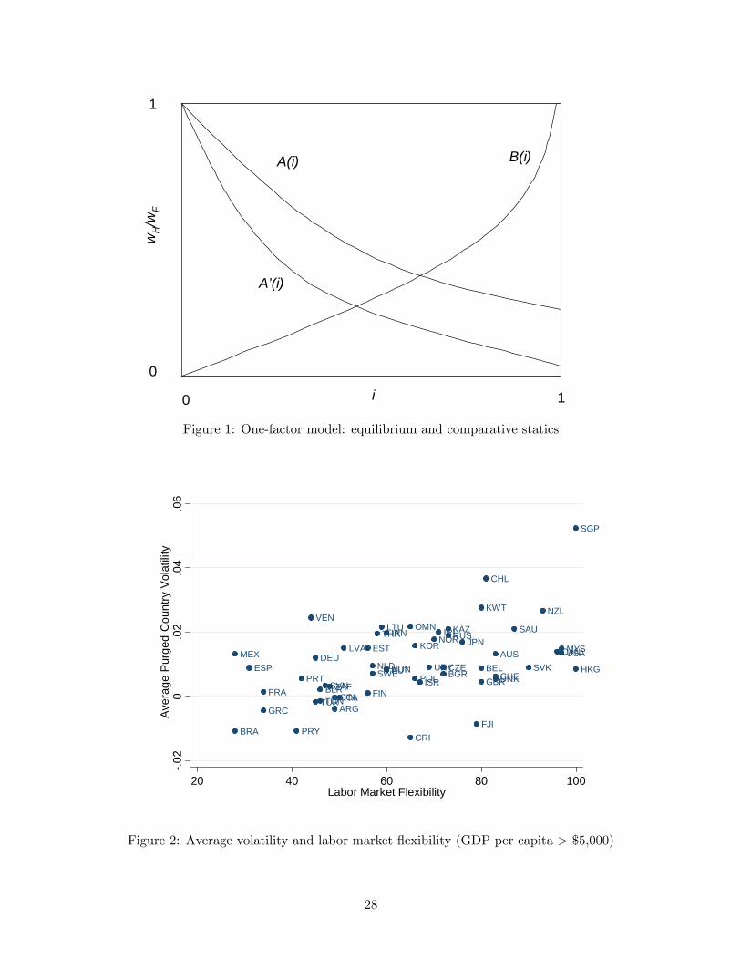
Lastly, we turn to the second approach discussed above. We use all the previously used
sector-level measures (K_s, S_s, VOL_AGG_s), as well as measures of the intensity of inter-
mediate goods (material cost per worker) and energy use (energy spending per worker). We run
an initial regression of VOL_s on all these sector level controls, and construct the residual as
VOL_PURGED_s (its correlation coe¢ cient with VOL_s is .93). Table 9 reports the correla-
tion coe¢ cients (which are also the standardized beta coe¢ cients) between VOL_PURGED_c
28One other advantage of this country-level method is that, unlike in the pooled country-sector analysis above, itdoes not require a monotonic response in a country�s share of exports across sectors to detect a pattern of comparativeadvantage.29We introduce the capital stock per worker variable in logs, since it varies by an order of magnitude greater than
for the other independent country-level variables. Entering this control in levels instead does not substantially changethe results.
19

and FLEX_c across all the country samples from Table 8, including an additional group of OECD
countries (with membership in the 1990s).30 As the table results clearly show, there is a very strong
correlation between country-level �exibility and this average volatility, across all sub-samples of
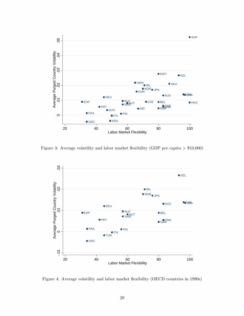
countries: all correlation coe¢ cients are signi�cant well beyond the 1% level. Figures 2-4 show the
scatter plots for these relationships for di¤erent country samples.
5 Concluding Remarks
Comparative advantage can arise even when the genuine production capabilities (resources and
technologies) of countries are identical, provided they di¤er in labor market institutions. Countries
with more �exible labor markets should display a comparative advantage precisely where the ability
to adjust is more important, that is, industries subject to high-variance shocks. The empirical
evidence presented above supports the validity of this intuition for a large sample of countries:
more �exible countries export relatively more in high volatility industries.
This result has some interesting implications. First, labor market reform is likely to have
asymmetric e¤ects across industries. Second, a rigid economy has an alternative to the liberalization
of its labor market to improve its welfare: it can always liberalize trade and �import �exibility�from
a more �exible trading partner. Finally, an extension of the model might provide an additional
explanation for the outsourcing phenomenon: production of intermediate goods may be relocated
to more �exible labor markets in high-volatility industries.
References
[1] Aghion, P., R. Burgess, S.J. Redding, and F. Zilibotti (2006): �The Unequal E¤ects of Liber-alization: Evidence from Dismantling the License Raj in India,�NBER WP 12031.
[2] Baldwin, R.E. (1971): �Determinants of the Commodity Trade Structure of US Trade,�Amer-ican Economic Review, 61(1), pp. 147-159.
[3] Baldwin, R.E. (1979): �Determinants of Trade and Foreign Investment: Further Evidence,�Review of Economics and Statistics, 61(1), pp. 40-48.
[4] Barro, R.J. and J.W. Lee (2000): �International Data on Educational Attainment Updatesand Implications,�NBER WP 7911.
[5] Bernard, A.B., S.J. Redding, and P.K. Schott (2006): �Comparative Advantage and Hetero-geneous Firms,�Review of Economic Studies, forthcoming.
30We can use this much smaller sample of countries since we are not losing any degrees of freedom with additionalco-variates.
20

[6] Bertola, G., and R. Rogerson (1997): �Institutions and Labor Reallocation,�European Eco-nomic Review 41 (6), pp. 1147-71.
[7] Blanchard, O. and P. Portugal (2001): �What Hides behind an Unemployment Rate: Com-paring Portuguese and US Labor Markets,�American Economic Review, 91(1), pp. 187-207.
[8] Botero, J., S. Djankov, R. La Porta, F. López de Silanes, and A. Shleifer (2004): �The Regu-lation of Labor,�Quarterly Journal of Economics, 119(4), pp. 1339-1382.
[9] Brecher, R.A. (1974a): �Minimum Wage Rates and the Pure Theory of International Trade,�Quarterly Journal of Economics, 88(1), pp. 98-116.
[10] Brecher, R.A. (1974b): �Optimal Commercial Policy for a Minimum-Wage Economy,�Journalof International Economics, 4(2), pp. 139-149.
[11] Broda, C., and D. E. Weinstein (2006): �Globalization and the Gains from Variety,�QuarterlyJournal of Economics 121(2), pp. 541-85.
[12] Brügemann, B. (2003): �Trade Integration and the Political Support for Labor Market Rigid-ity,�manuscript, Yale.
[13] Costinot, A. (2005): �Contract Enforcement, Division of Labor, and the Pattern of Trade,�manuscript, UCSD.
[14] Davidson, C., L. Martin, and S. Matusz (1999): �Trade and Search Generated Unemployment,�Journal of International Economics, 48, pp. 271-299.
[15] Davis, D.R. (1998a): �Does European Unemployment Prop up American Wages? NationalLabor Markets and Global Trade,�American Economic Review, 88(3), pp. 478-494.
[16] Davis, D.R. (1998b): �Technology, Unemployment, and Relative Wages in a Global Economy,�European Economic Review, 42, pp. 1613-1633.
[17] Davis, S.J., J.C. Haltiwanger, and S. Schuh (1997): Job Creation and Destruction, MIT Press.
[18] di Giovanni, J. and A.A. Levchenko (2006): �The Risk Content of Exports,�manuscript, IMF.
[19] Dornbusch, R., S. Fischer, and P.A. Samuelson (1977): �Comparative Advantage, Trade, andPayments in a Ricardian Model with a Continuum of Goods,�American Economic Review,67(5), pp. 823-839.
[20] Feenstra, R.C., R.E. Lipsey, H. Deng, A.C. Ma, and H. Mo (2005): �World Trade Flows,�NBER WP 11040.
[21] Galdón-Sánchez, J.E. (2002): �Employment Protection Legislation and the IT-Sector in OECDCountries,�Recherches Économiques de Louvain, 68(1-2), pp. 21-36.
[22] Haaland, J.I. and I. Wooton (2006): �Domestic Labour Markets and FDI,�Review of Inter-national Economics, forthcoming.
[23] Koren, M. and S. Tenreyro (2005): �Volatility and Development,�Quarterly Journal of Eco-nomics, forthcoming.
[24] Levchenko, A.A. (2004): �Institutional Quality and International Trade,�IMF WP/04/231.
21

[25] Matusz, S.J. (1996): �International Trade, the Division of Labor, and Unemployment�Inter-national Economic Review, 37(1), pp. 71-84.
[26] Nunn, Nathan (2005): �Relationship-Speci�city, Incomplete Contracts, and the Pattern ofTrade,�Quarterly Journal of Economics, forthcoming.
[27] OECD Employment Outlook (1999): �Employment Protection and Labour Market Perfor-mance�, Chapter 2, OECD.
[28] Romalis, J. (2004): �Factor Proportions and the Structure of Commodity Trade,�AmericanEconomic Review, 94(1), pp. 67-97.
[29] Saint-Paul, G. (1997): �Is Labour Rigidity Harming Europe�s Competitiveness? The E¤ectof Job Protection on the Pattern of Trade and Welfare,�European Economic Review, 41, pp.499-506.
22
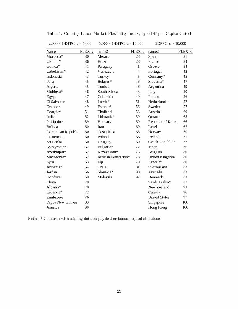
Table 1: Country Labor Market Flexibility Index, by GDP per Capita Cuto¤
Name FLEX_c name2 FLEX_c name2 FLEX_cMorocco* 30 Mexico 28 Spain 31Ukraine* 36 Brazil 28 France 34Guinea* 41 Paraguay 41 Greece 34Uzbekistan* 42 Venezuela 44 Portugal 42Indonesia 43 Turkey 45 Germany* 45Peru 45 Belarus* 46 Slovenia* 47Algeria 45 Tunisia 46 Argentina 49Moldova* 46 South Africa 48 Italy 50Egypt 47 Colombia 49 Finland 56El Salvador 48 Latvia* 51 Netherlands 57Ecuador 49 Estonia* 56 Sweden 57Georgia* 51 Thailand 58 Austria 60India 52 Lithuania* 59 Oman* 65Philippines 59 Hungary 60 Republic of Korea 66Bolivia 60 Iran 60 Israel 67Dominican Republic 60 Costa Rica 65 Norway 70Guatemala 60 Poland 66 Ireland 71Sri Lanka 60 Uruguay 69 Czech Republic* 72Kyrgyzstan* 62 Bulgaria* 72 Japan 76Azerbaijan* 62 Kazakhstan* 73 Belgium 80Macedonia* 62 Russian Federation* 73 United Kingdom 80Syria 63 Fiji 79 Kuwait* 80Armenia* 64 Chile 81 Switzerland 83Jordan 66 Slovakia* 90 Australia 83Honduras 69 Malaysia 97 Denmark 83China 70 Saudi Arabia* 87Albania* 70 New Zealand 93Lebanon* 72 Canada 96Zimbabwe 76 United States 97Papua New Guinea 83 Singapore 100Jamaica 90 Hong Kong 100
2,000 < GDPPC_c = 5,000 5,000 < GDPPC_c = 10,000 GDPPC_c > 10,000
Notes: * Countries with missing data on physical or human capital abundance.
23

Table 2: Job Reallocation: Comparing US and Portugal
Quarterly job creation and destruction, all manufacturing sectors
(Source: Blanchard and Portugal (2001))
Job Creation Job Destruction Job Reallocation
Portugal 4 3.9 7.9(1991:11995:4)
US 6.8 7.3 14(1972:21993:4)
Table 3: Variation in Job Reallocation Rates Across Sectors
Average annual excess job reallocation rates,US manufacturing sectors
(Source: Davis, Haltiwanger, and Schuh (1997))
Percentile Excess Job Reallocation
1% 4.15% 6.210% 7.425% 9.950% 12.975% 15.890% 19.495% 21.799% 25.6
SizeWeighted Mean 13.2Industry Observations 514
24

Table 4: The Ten Least and Most Volatile Sectors at the 3-Digit SIC Level
SIC3 VOL_s # firms Description203 0.084 33 Preserved Fruits & Vegetables386 0.096 42 Photographic Equipment & Supplies285 0.097 16 Paints & Allied Products271 0.100 24 Newspapers276 0.103 15 Manifold Business Forms358 0.103 52 Refrigeration & Service Machinery267 0.105 48 Misc. Converted Paper Products342 0.105 24 Cutlery, Handtools, & Hardware314 0.112 25 Footwear, Except Rubber327 0.115 25 Concrete, Gypsum, & Plaster Products
SIC3 VOL_s # firms Description333 0.236 20 Primary Nonferrous Metals302 0.247 10 Rubber & Plastics Footwear355 0.255 104 Special Industry Machinery274 0.262 16 Miscellaneous Publishing332 0.263 13 Iron & Steel Foundries346 0.265 20 Metal Forgings & Stampings202 0.287 17 Dairy Products369 0.300 59 Misc. Electrical Equipment & Supplies367 0.306 316 Electronic Components & Accessories361 0.336 17 Electric Distribution Equipment
Table 5: Pooled Regression �Baseline
SIC aggregation SIC4 SIC3 SIC4 SIC3GDPPC cutoff 2000 2000 5000 5000VOL_s * log FLEX_c 0.300 0.298 0.356 0.382
(0.060) *** (0.073) *** (0.070) *** (0.083) ***log K_s * log FLEX_c 0.239 0.300 0.173 0.223
(0.069) *** (0.094) *** (0.080) ** (0.114) *log K_s * log K_c 0.773 1.055 0.546 1.057
(0.092) *** (0.119) *** (0.169) *** (0.232) ***log S_s * log S_c 0.802 0.961 0.822 0.973
(0.063) *** (0.091) *** (0.077) *** (0.102) ***Observations 13203 6513 9739 4675Rsquared 0.7016 0.7481 0.6913 0.7472
Notes: Beta coe¢ cients are reported. Country and sector dummies suppressed. Heteroskedasticity robuststandard errors in parentheses. * signi�cant at 10%; ** signi�cant at 5%; *** signi�cant at 1%
25

Table 6: Pooled Regression �Including Obsevations with No Exports
SIC aggregation SIC4 SIC3 SIC4 SIC3GDPPC cutoff 2000 2000 5000 5000VOL_s * log FLEX_c 0.097 0.165 0.113 0.189
(0.039) ** (0.059) *** (0.038) *** (0.060) ***log K_s * log FLEX_c 0.168 0.141 0.162 0.121
(0.039) *** (0.063) ** (0.041) *** (0.069) *log K_s * log K_c 0.803 0.800 0.829 0.737
(0.050) *** (0.082) *** (0.085) *** (0.148) ***log S_s * log S_c 0.286 0.353 0.242 0.424
(0.041) *** (0.065) *** (0.040) *** (0.062) ***Observations 22753 8235 14574 5544Rsquared 0.8041 0.8288 0.8564 0.8667
Notes: Beta coe¢ cients are reported. Country and sector dummies suppressed. Heteroskedasticity robuststandard errors in parentheses. * signi�cant at 10%; ** signi�cant at 5%; *** signi�cant at 1%. Allpotential country-sector combinations are represented.
Table 7: Pooled Regression �Robustness Checks
SIC aggregation SIC3 SIC3 SIC3 SIC3 SIC3 SIC3GDPPC cutoff 2000 5000 2000 5000 2000 5000VOL_s * log FLEX_c 0.289 0.374 0.304 0.373 0.246 0.283
(0.073) *** (0.083) *** (0.074) *** (0.084) *** (0.088) *** (0.110) ***log K_s * log FLEX_c 0.297 0.219 0.323 0.218 0.307 0.245
(0.094) *** (0.114) * (0.094) *** (0.112) * (0.095) *** (0.121) **log K_s * log K_c 1.155 1.139 1.165 1.138 1.258 0.177
(0.123) *** (0.236) *** (0.123) *** (0.236) *** (0.541) ** (0.745)log S_s * log S_c 0.936 0.959 0.938 0.959 0.445 0.299
(0.091) *** (0.102) *** (0.091) *** (0.102) *** (0.148) *** (0.144) **VOLPROD_AGG_s * log GDPPC_c 0.287 0.238 0.314 0.235 0.274 0.138
(0.097) *** (0.177) (0.099) *** (0.193) (0.100) *** (0.195)VOL_AGG_s * log FLEX_c 0.124 0.005 0.111 0.031
(0.102) (0.127) (0.103) (0.128)VOL_s * log K_c 0.463 1.608
(0.434) (0.679) **VOL_s * log S_c 0.077 0.056
(0.077) (0.089)VOL_s * log GDPPC_c 0.344 0.966
(0.340) (0.546) *log K_s * log GDPPC_c 0.115 0.720
(0.429) (0.612)log S_s * log GDPPC_c 0.805 1.333
(0.170) *** (0.235) ***Observations 6513 4675 6513 4675 6513 4675Rsquared 0.7487 0.7474 0.7488 0.7474 0.7499 0.7502
Notes: Beta coe¢ cients are reported. Country and sector dummies suppressed. Heteroskedasticity robuststandard errors in parentheses. * signi�cant at 10%; ** signi�cant at 5%; *** signi�cant at 1%.
26

Table 8: Country-Level Analysis
GDPPC cutoff 10000 5000 2000 NONE (weighted)FLEX_c 0.820 0.574 0.292 0.275
(0.259) *** (0.169) *** (0.137) ** (0.109) **GDPPC_c 0.394 0.657 0.212 0.259
(0.412) (0.428) (0.361) (0.183)S_c 0.215 0.216 0.187 0.341
(0.207) (0.205) (0.208) (0.178) *log K_c 0.469 1.052 0.382 0.259
(0.337) (0.412) ** (0.361) (0.235)Observations 25 42 61 81Rsquared 0.4728 0.4354 0.2744 0.4690
Notes: Beta coe¢ cients are reported. Standard errors in parentheses. * signi�cant at 10%; ** signi�cant at5%; *** signi�cant at 1%. Last column is weighted by RGDP
Table 9: Country-Level Analysis: Correlation between Purged Average Volatility and CountryFlexibility
OECD 10000 5000 2000 NONE (weighted)0.6197 0.5511 0.4591 0.3295 0.4918
(0.0027) (0.0013) (0.0004) (0.0018) (0.0000)Observations 21 31 56 87 121
Notes: Correlation coe¢ cients are reported. p-values in parentheses. * signi�cant at 10%; ** signi�cant at5%; *** signi�cant at 1%. Last column is weighted by RGDP
27
wH/w
F
1
0
0 1i
B(i)A(i)
A’(i)
Figure 1: One-factor model: equilibrium and comparative statics
ARG
AUS
AUT BELBGR
BLR
BRA
CAN
CHE
CHL
COL
CRI
CZEDEU
DNKESP
EST
FIN
FJI
FRAGBR
GRC
HKGHUN
IRLIRN
ISR
ITA
JPNKAZ
KOR
KWT
LTU
LVAMEX MYS
NLD
NOR
NZL
OMN
POLPRT
PRY
RUSSAU
SGP
SVK
SVNSWE
THA
TUNTUR
URYUSA
VEN
ZAF
.02
0.0
2.0
4.0
6A
vera
ge P
urge
d C
ount
ry V
olat
ility
20 40 60 80 100Labor Market Flexibility
Figure 2: Average volatility and labor market �exibility (GDP per capita > $5,000)
28
ARG
AUS
AUT BEL
CAN
CHECZE
DEU
DNK
ESP
FINFRAGBR
GRC
HKG
IRL
ISR
ITA
JPNKOR
KWT
NLD
NOR
NZL
OMN
PRT
SAU
SGP
SVN
SWE
USA
0.0
1.0
2.0
3.0
4.0
5A
vera
ge P
urge
d C
ount
ry V
olat
ility
20 40 60 80 100Labor Market Flexibility
Figure 3: Average volatility and labor market �exibility (GDP per capita > $10,000)
AUS
AUT BEL
CANDEU
DNK
ESP
FINFRA
GBR
GRC
IRL
ITA
JPN
NLD
NOR
NZL
PRTSWE
TUR
USA
.01
0.0
1.0
2.0
3A
vera
ge P
urge
d C
ount
ry V
olat
ility
20 40 60 80 100Labor Market Flexibility
Figure 4: Average volatility and labor market �exibility (OECD countries in 1990s)
29

Appendix
A Two-Factor Model: Autarky in the Flexible Country
Since the rental rate and the allocation of capital are pre-determined prior to the realization of �, all
intermediate good producers in an industry hire the same amount of capital: Kc(i; �) = Kc (i) ; 8�,
where Kc (i) is also the total amount of capital hired in the industry (since there is a unit mass of
intermediate good producers).31 Hence,
y(�)
y(0)= e�
�L(�)
L(0)
�1��: (A.1)
Market clearing for each �rm�s output y(�) and price p(�) implies
y(�)
y(0)=
�p(�)
p(0)
��": (A.2)
Firms hire labor until the value of its marginal product is equal to the common wage:
w = � (�) p(�) (1� �) e�K�L (�)�� ; (A.3)
where � (�) = ��� (1� �)��1. Equations (A.1), (A.2) and (A.3) yield
p(�)
p(0)= exp
���
1 + � ("� 1)
�; (A.4)
andL(�)
L(0)= exp
�("� 1)
1 + � ("� 1)��: (A.5)
Equations (A.2) and (A.4) imply
p(�)y(�)
p(0)y(0)= exp
�("� 1)
1 + � ("� 1)��: (A.6)
Since labor is paid the value of its marginal product, the Cobb-Douglas production form (and
zero pro�t condition) implies that each �rm pays a share (1� �) of its revenue p(�)y(�) to labor:
wL(�) = (1� �) p(�)y(�). This relationship also holds in the aggregate for the industry: wL =31 In what follows, country and industry notation is suppressed for simplicity wherever unnecessary. It is understood
that � and � will vary across industries.
A-1

(1� �) py. As there are no ex-ante pro�ts, wages are determined so that aggregate capital cost rK
equals the remaining � share of revenue:
rK = �
Z 1
�1p(�)y(�)dF (�) = �p(0)y(0) exp
(�("� 1)
1 + � ("� 1)
�2 �22
): (A.7)
Using expressions w = � (�) (1� �) p(0) [K=L (0)]� and wL(0) = (1� �) p(0)y(0), which imply
that p(0)y(0) = [� (�)]1=� [w= (1� �)](��1)=� p(0)1=�K, equation (A.7) can be written as
r�w1�� = p(0) exp
(�
�("� 1)
1 + � ("� 1)
�2 �22
); (A.8)
where the left-hand side is the standard Cobb-Douglas unit cost function. Finally, note that (A.4)
implies that the price index for the �nal good is given by
p = p(0) exp
(��
("� 1)1 + � ("� 1)
�2 1
"� 1�2
2
):
Solving out for p(0) using equation (A.8) yields
p = exp
�� ("� 1)1 + � ("� 1)
�2
2
�r�w1��:
One can think of our static set-up as a steady-state equilibrium: the law of large numbers ensures
that aggregate outcomes are invariant over time, but the realizations of � experienced by an in-
dividual �rm vary from period to period. Assume � is iid over time. From equation (A.6), the
growth rate of a �rm�s sales between periods t and t0 can be expressed as
� log p (�0) y (�0)
p (�) y (�)=("� 1) (�0 � �)1 + � ("� 1) :
The standard deviation of is therefore
volF (i; j) =
p2 ("� 1)
1 + � (j) ("� 1)� (i) : (A.9)
The one-factor/�exible-country counterpart to equation (A.9) can be obtained by assuming � (j) =
0: volF (i) =p2 ("� 1)� (i). Assuming � (j) = 1 yields the case of a one-factor model in which the
factor is �rigid�: volF (i) =p2 ("� 1)� (i) =". In the two-factor/rigid-country case, we can think
A-2

of the two rigid factors as combining into a composite rigid factor. The prediction for volatility is
obviously the same in this case:
volH (i; j) =
p2 ("� 1)"
� (i) < volF (i; j) : (A.10)
Not surprisingly, �rm sales in the rigid country vary less than in the �exible country, as �rms cannot
adjust their employment in the rigid country.
B Three Factors
Assume now that countries use three factors in the production of intermediates: a �rigid�factor,
capital, a ��exible�factor, materials, and labor. Industries di¤er in terms of factor intensities and
volatility. The Cobb-Douglas aggregate good Q is now de�ned according to
Q � exp�Z 1
0
Z 1
0
Z 1
0ln q (i; j;m) didjdm
�;
where an industry is now characterized by a triple (i; j;m). The �nal good in each industry is still
produced from a C.E.S. continuum of intermediate goods indexed by z:
y (i; j;m) =
�Z 1
0y (i; j;m; z)
"�1" dz
� ""�1
;
Intermediate goods are now produced with capital, materials, and labor, according to
y (i; j;m; z) = e��K(i; j;m; z)
� (j)
��(j) �M(i; j;m; z)� (m)
��(m) � L(i; j;m; z)
1� � (j)� � (m)
�1��(j)��(m);
where � (j) ; � (m) ; 1�� (j)�� (m) 2 [0; 1] are the industry�s cost shares of capital, materials, and
labor, respectively. As in the one-factor model, the �0s are iid draws from a common distribution,
identical across countries, but di¤erent across industries. We maintain the Normal parametrization
for the productivity draws � (i) � N�0; �2 (i)
�. Labor market �exibility varies across countries in
the same way as above. We assume that in both countries, the rental rate and the allocation of
capital to intermediate good producers are determined prior to the realization of �; no adjustment
is allowed thereafter. Materials are instead allocated after the realization of � in both countries.
A-3

Autarky in the Flexible Country
This case is similar to the two-factor model with �exible labor and rigid capital: we can rewrite
the �rm-level production function as
y (i; j;m; z) = e��K(i; j;m; z)
� (j)
��(j) 24�M(i; j;m; z)� (m)
� �(m)1��(j)
�L(i; j;m; z)
1� � (j)� � (m)
� 1��(j)��(m)1��(j)
351��(j) ;where the term in brackets can be understood as a composite �exible factor, and K as a rigid
factor. Therefore,
pF (i; j;m) =r�(j)F s
�(m)F w
1��(j)��(m)F
~�F (i; j;m);
where s denotes the price of materials, the numerator is the standard Cobb-Douglas unit cost
function, and the industry average productivity level ~�F (i; j;m) is now given by
~�F (i; j;m) = exp
�"� 1
1 + � (j) ("� 1)�2 (i)
2
�:
From the two-factor analysis above, we also know
volF (i; j;m) =
p2 ("� 1)� (i)
1 + � (j) ("� 1) : (B.1)
Autarky in the Rigid Country
We can rewrite the �rm-level production function as
y (i; j;m; z) = e��M(i; j;m; z)
� (m)
��(m) 24�K(i; j;m; z)� (j)
� �(j)1��(m)
�L(i; j;m; z)
1� � (j)� � (m)
� 1��(j)��(m)1��(m)
351��(m) ;where the term in brackets can be understood as a composite rigid factor, and M as a �exible
factor. Therefore,
pH (i; j;m) =r�(j)H s
�(m)H w
1��(j)��(m)H
~�H(i; j;m);
where the industry average productivity level ~�H(i; j;m) is now given by
~�H(i; j;m) = exp
�("� 1)
1 + [1� � (m)] ("� 1)�2 (i)
2
�:
A-4
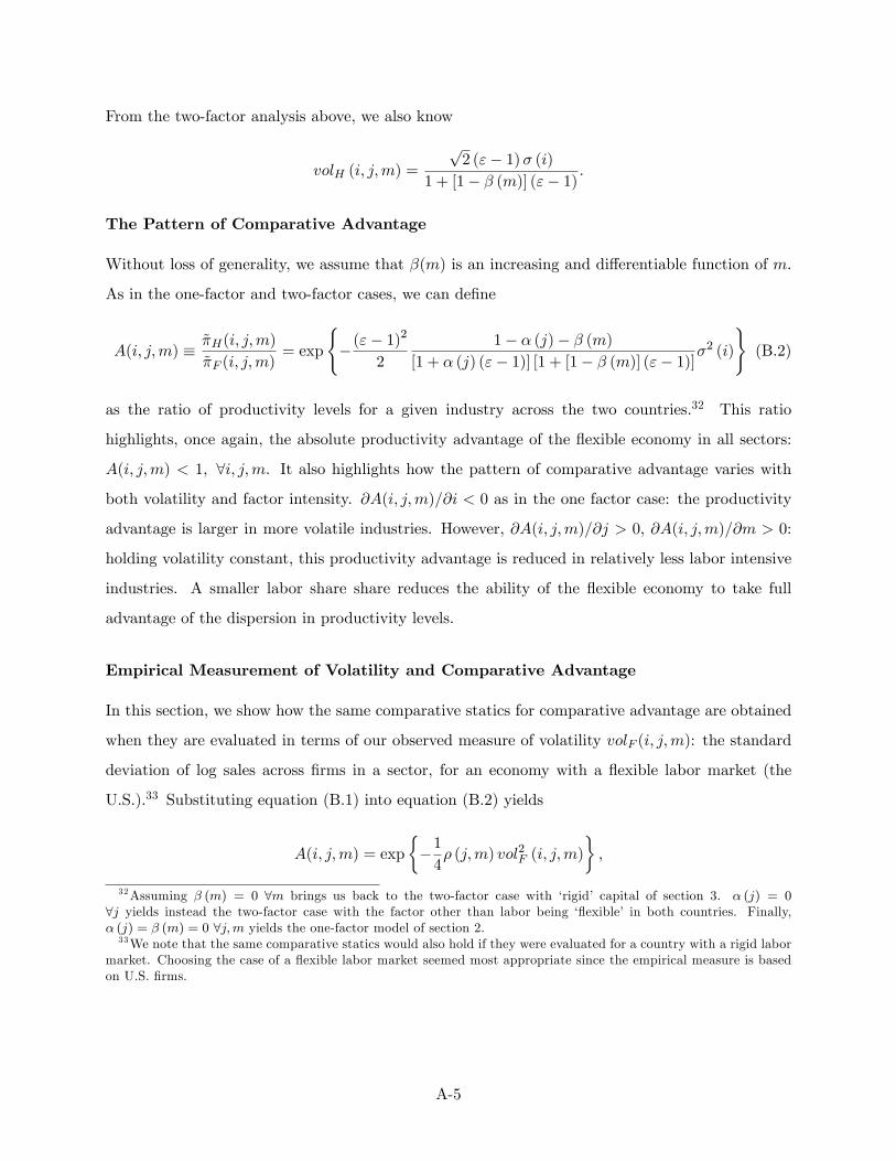
From the two-factor analysis above, we also know
volH (i; j;m) =
p2 ("� 1)� (i)
1 + [1� � (m)] ("� 1) :
The Pattern of Comparative Advantage
Without loss of generality, we assume that �(m) is an increasing and di¤erentiable function of m.
As in the one-factor and two-factor cases, we can de�ne
A(i; j;m) � ~�H(i; j;m)
~�F (i; j;m)= exp
(�("� 1)
2
2
1� � (j)� � (m)[1 + � (j) ("� 1)] [1 + [1� � (m)] ("� 1)]�
2 (i)
)(B.2)
as the ratio of productivity levels for a given industry across the two countries.32 This ratio
highlights, once again, the absolute productivity advantage of the �exible economy in all sectors:
A(i; j;m) < 1; 8i; j;m. It also highlights how the pattern of comparative advantage varies with
both volatility and factor intensity. @A(i; j;m)=@i < 0 as in the one factor case: the productivity
advantage is larger in more volatile industries. However, @A(i; j;m)=@j > 0; @A(i; j;m)=@m > 0:
holding volatility constant, this productivity advantage is reduced in relatively less labor intensive
industries. A smaller labor share share reduces the ability of the �exible economy to take full
advantage of the dispersion in productivity levels.
Empirical Measurement of Volatility and Comparative Advantage
In this section, we show how the same comparative statics for comparative advantage are obtained
when they are evaluated in terms of our observed measure of volatility volF (i; j;m): the standard
deviation of log sales across �rms in a sector, for an economy with a �exible labor market (the
U.S.).33 Substituting equation (B.1) into equation (B.2) yields
A(i; j;m) = exp
��14� (j;m) vol2F (i; j;m)
�;
32Assuming � (m) = 0 8m brings us back to the two-factor case with �rigid� capital of section 3. � (j) = 08j yields instead the two-factor case with the factor other than labor being ��exible� in both countries. Finally,� (j) = � (m) = 0 8j;m yields the one-factor model of section 2.33We note that the same comparative statics would also hold if they were evaluated for a country with a rigid labor
market. Choosing the case of a �exible labor market seemed most appropriate since the empirical measure is basedon U.S. �rms.
A-5

where
� (j;m) =[1� � (j)� � (m)] [1 + � (j) ("� 1)]
[1 + [1� � (m)] ("� 1)] > 0:
Thus, the comparative statics for A(i; j;m) in terms of volF are identical to those in terms of �2(i):
relative productivity A(i; j;m) varies negatively with volatility for both measures. We now turn
to the secondary e¤ect of labor market �exibility based on variations in factor intensities. Some
tedious algebra yields
@� [� (j) ; � (m)]
@� (j)=("� 1) [1� 2� (j)� � (m)]� 1
[(1� � (m)) "+ � (m)] ;
@� [� (j) ; � (m)]
@� (m)= �
�� (j) "+ 1� � (j)
(1� � (m)) "+ � (m)
�2:
Clearly, @� [� (j) ; � (m)] =@� (m) < 0. Although the sign of @� [� (j) ; � (m)] =@� (j) is analytically
ambiguous, we document that this derivative is negative for virtually all empirical measures of �(j)
and �(m) across sectors, combined with plausible values for ". @� [� (j) ; � (m)] =@� (j) < 0 if and
only if
2�(j) + �(m) >"� 2"� 1 : (B.3)
The RHS of (B.3) is increasing in ". Even for an upper-bound value for " of 10, the RHS is below
:9.34 We can evaluate the empirical distribution of the LHS of (B.3) across all U.S. SIC sectors
that we use in our empirical analysis. We use expenditures on energy and materials as a share
of the gross value of production to represent �(m). We compute a similar share for expenditures
on labor, and compute �(j) as the residual share, 1 minus the sum of the other shares (labor and
�(m)). At the SIC-3 level, the LHS for all sectors is bounded below by .9. At the SIC-4 level, 98%
of sectors have a LHS value above .9. Thus, empirically, (B.3) will be satis�ed for all SIC-3 sectors
and almost all the SIC-4 sectors. We therefore conclude that our secondary comparative statics
also hold when evaluated in terms of our empirical measure of volatility, volF .
C Degrees of Flexibility/Rigidity
A simple way of introducing di¤erent degrees of labor market �exibility/rigidity is to assume that
each industry is comprised of both �exible and rigid sub-industries �henceforth sectors �and thus
34Virtually all micro-level studies measuring elasticities of substitution (or cross-price elasticities) within sectors�nd estimates substantially below 10 (except for very rare cases of a few special commodity goods). One of the mostcomprehensive such study, using data on prices across export origins by Broda and Weinstein (2006), �nds a medianprice elasticity of 2.5 within all traded 3-digit SITC sectors (the standard error across the 327 di¤erent sectors is 1.2).
A-6

introducing one additional layer of aggregation into the model. For simplicity, we will work out the
one-factor case. The extension to the many-factor case is immediate.
We maintain most of our assumptions from the main text. We now think of each industry i as
an aggregate of nontraded sectors s:
y (i) = exp
�Z 1
0ln y (i; s) ds
�;
where y (i) denotes production of �nal good i. Each good s is produced with a continuum of
nontraded intermediate goods:
y (i; s) =
�Z 1
0y (i; s; z)
"�1" dz
� ""�1
:
Each intermediate good is produced with labor y (i; s; z) = e�L (i; s; z). An economy-wide wage
w is chosen before uncertainty is realized. We assume that the unemployed cannot bid down this
wage. Within each industry, there are ��exible� and �rigid� sectors. We assume that a measure
� 2 [0; 1] of sectors in industry i are �exible, whereas a measure (1� �) are rigid. Labor is ex-ante
perfectly mobile across sectors and industries.
In a �exible sector, �rms hire labor after uncertainty is realized. After the realization of �,
production and commodity market clearing take place in a competitive setting. Rigid sectors
must hire labor before uncertainty is realized, and the intermediate good producer is contractually
committed to paying the hired number of workers the negotiated wage (regardless of the realization
of �). After the realization of �, production and commodity market clearing take place in a
competitive setting, subject to the wage and employment restrictions. Rigid-sector intermediate
goods producers anticipate this equilibrium, and adjust their contracted labor demand accordingly.
Given ex-ante free entry into the intermediate goods sector, expected pro�ts of the rigid-sector
intermediate good producers are driven to zero.
Autarky
For s 2 [0; �],
~�(i; s) =
�Z 1
�1e("�1)�dGi (�)
� 1"�1
;
A-7

whereas for s 2 [�; 1],
~�(i; s) =
�Z 1
�1e("�1)"
�dGi (�)
� ""�1
:
In both cases, p(i; s) = w=~�(i; s). Given the absolute advantage of �exible sectors over rigid sectors,
an industry�s price index is a negative function of �. Assuming � � N�0; �2
�, the industry�s price
index is p(i) = w=~�(i), where
~� (i) = exp
("("� 1)2
"�+
("� 1)"
#�2 (i)
2
)
is the combined productivity average for industry i.
Free Trade
Assume �F > �H . De�ne
A(i) � ~�H(i)
~�F (i)= exp
(�("� 1)
2
2"(�F � �H)�2 (i)
):
As in the one-factor model in the main text, the full-employment free-trade equilibrium can be
characterized by the intersection of A (i) and B (i). Notice that an increase in �F � �H will have
e¤ects similar to a proportional increase in �2 (i) for all i. (In other words, �F � �H operates like
.)
Consider now the case with unemployment, and again normalize wF = 1. The condition wH =
A (�{) still determines the equilibrium specialization pattern: �{ = �{ (wH ; �F � �H). Again, since
@A (�) =@i < 0, d�{=dwH < 0. Goods market clearing requires wHLH=LF =
�{ (wH ; �F � �H) = [1� �{ (wH ; �F � �H)] � B (wH ; �F � �H), where B (�) depends negatively on
wH . It is easy to see that country H�s employment level (relative to country F�s) depends neg-
atively on wH : LH=LF = B (wH ; �F � �H) =wH , @ (LH=LF ) =@wH < 0. Finally, an increase in
�F � �H (or a proportional increase in �2 (i) for all i) will shift LH=LF down for a given wH :
@ (LH=LF ) =@ (�F � �H) < 0.
A-8


