201
© 2016 Maryam Kazerooni

© 2016 Maryam Kazerooni
ENHANCED POWER SYSTEM RESILIENCY TO HIGH-IMPACT, LOW-FREQUENCY EVENTSWITH EMPHASIS ON GEOMAGNETIC DISTURBANCES
BY
MARYAM KAZEROONI
DISSERTATION
Submitted in partial fulfillment of the requirementsfor the degree of Doctor of Philosophy in Electrical and Computer Engineering
in the Graduate College of theUniversity of Illinois at Urbana-Champaign, 2016
Urbana, Illinois
Doctoral Committee:
Professor Thomas J. Overbye, ChairProfessor Peter W. SauerProfessor Deming ChenAssistant Professor Hao ZhuDr. James D. Weber, PowerWorld Corporation

ABSTRACT
Various reliability procedures have been developed to protect the power systems against common
reliability issues that threaten the grid frequently. However, these procedures are unlikely to be
sufficient for high-impact low-frequency (HILF) events. This thesis proposes several techniques
to enhance resiliency with respect to HILF events. In particular, we focus on cyber-physical at-
tacks and geomagnetic disturbances (GMDs). Corrective control through generation redispatch is
proposed to protect the system from cyber-physical attacks. A modification of the optimal power
flow (OPF) is proposed which optimizes the system resiliency instead of the generation cost. For
larger systems, the burden of solving the resilience-oriented OPF is reduced through a fast greedy
algorithm which utilizes proper heuristics to narrow the search space. Moreover, an effective line
switching algorithm is developed to minimize the GMD impact for large-scale power systems.
The algorithm uses linear sensitivity analysis to find the best switching strategy and minimizes the
GIC-saturated reactive power loss.
The resiliency may be improved through power system monitoring and situational awareness.
Power system data is growing rapidly with the everyday installation of different types of sensors
throughout the network. In this thesis, various data analytics tools are proposed to effectively
employ the sensor data for enhancing resiliency. In particular, we focus on the application of
real data analysis to improve the GMD models. We identify common challenges in dealing with
real data and develop effective tools to tackle them. A frequent issue with model validation is
that for a real system, the parameters of the model to be validated may be inaccurate or even
unavailable. To handle this, two approaches are proposed. The first approach is to develop a
validation framework which is independent of the model parameters and completely relies on the
measurements. Although this technique successfully handles the system uncertainties and offers
a robust validation tool, it does not provide the ability to utilize the available network parameters.
ii

Sometimes, the network parameters are partially available with some degree of accuracy and it is
desired to take advantage of this additional information. The second validation framework provides
this capability by first modifying the model to account for the missing or inaccurate parameters.
Then a suitable validation framework is built upon that model. Another common issue that is
widely encountered in data analysis techniques is incomplete data when part of the required data
is missing or is invalid. Examples of missing data are provided through real case studies, and
advanced imputation tools are developed to handle them.
iii

To my parents, for their love and support.
iv

ACKNOWLEDGMENTS
Throughout the course of my Ph.D., I am grateful to those with whom I have had the opportunity
to collaborate and all who have taught or mentored me. First, and most sincerely, I thank my
advisor, Professor Tom Overbye, for his continual guidance and support throughout my graduate
academic career. I have learned a lot from him about power systems and how to do research. Many
thanks also go to my thesis committee for their interest, involvement, and encouragement of my
work. Additionally, I extend my sincere gratitude to Dr. Kate Davis, adjunct assistant professor at
the University of Illinois, and Dr. Saman Zonous, professor at Rutgers University, for their direct
guidance on the work in Chapter 2.
Throughout graduate school, I had the privilege of participating in a few industrial internships.
I extend thanks to all the mentors who guided me through these precious experiences: At MISO,
I learned about power systems planning from Stuart Hansen, Jordan Bakke and Aditya Prabhakar;
and at Fujitsu lab, I gained valuable experience in demand response and distribution systems under
the guidance of Jorjeta Jetcheva, Daisuke Mashima and Wei-Peng Chen.
There have been quite a few other people I have worked with, who have inspired me with
their support, encouragement, and advice. Thanks in particular to Jennifer Gannon, Shamina
Hossain-Mckenzie, Komal Shetye and Mark Butala. I would also like to acknowledge my funding
sources, the National Science Foundation (NSF), the Power Systems Engineering Research Center
(PSERC), and the Illinois Center for a Smarter Electric Grid (ICSEG).
Finally, I thank my family, who sacrificed much to provide a better life for me. They instilled in
me the value of hard work and discipline, the interest in mathematics and the belief that I could do
anything. Last, thanks to my husband, Arash, for his unconditional support.
v
TABLE OF CONTENTS
CHAPTER 1 INTRODUCTION . . . . . . . . . . . . . . . . . . . . . . . . . . . . . . . 11.1 Problem Statement . . . . . . . . . . . . . . . . . . . . . . . . . . . . . . . . . . 11.2 Background . . . . . . . . . . . . . . . . . . . . . . . . . . . . . . . . . . . . . . 21.3 Literature Review . . . . . . . . . . . . . . . . . . . . . . . . . . . . . . . . . . . 5
1.3.1 Generation Redispatch for Cyber Attacks . . . . . . . . . . . . . . . . . . 51.3.2 GMD Mitigation through Line Switching . . . . . . . . . . . . . . . . . . 61.3.3 GMD Model Validation Based on Real Data . . . . . . . . . . . . . . . . . 71.3.4 Substation Grounding Resistance Estimation . . . . . . . . . . . . . . . . 81.3.5 Enhanced Magnetic Field Estimation . . . . . . . . . . . . . . . . . . . . 101.3.6 Enhanced E-field Estimation . . . . . . . . . . . . . . . . . . . . . . . . . 101.3.7 Adding GMD Models to the Existing Test Cases . . . . . . . . . . . . . . 10
1.4 Contribution of Thesis . . . . . . . . . . . . . . . . . . . . . . . . . . . . . . . . 111.5 Thesis Organization . . . . . . . . . . . . . . . . . . . . . . . . . . . . . . . . . . 12
CHAPTER 2 GENERATION REDISPATCH DURING CYBER ATTACKS . . . . . . . . 162.1 Introduction . . . . . . . . . . . . . . . . . . . . . . . . . . . . . . . . . . . . . . 162.2 Related Work . . . . . . . . . . . . . . . . . . . . . . . . . . . . . . . . . . . . . 172.3 Power System Security Control . . . . . . . . . . . . . . . . . . . . . . . . . . . . 18
2.3.1 Remedial Action Schemes . . . . . . . . . . . . . . . . . . . . . . . . . . 192.4 Resilience-oriented OPF . . . . . . . . . . . . . . . . . . . . . . . . . . . . . . . 20
2.4.1 Security Constrained OPF . . . . . . . . . . . . . . . . . . . . . . . . . . 222.4.2 Proposed Resilience-oriented OPF . . . . . . . . . . . . . . . . . . . . . . 23
2.5 Security-compliant Control Subspace Synthesis . . . . . . . . . . . . . . . . . . . 252.5.1 The Proposed Violation Index . . . . . . . . . . . . . . . . . . . . . . . . 252.5.2 The Performance Improvements . . . . . . . . . . . . . . . . . . . . . . . 27
2.6 Simulation and Numerical Results . . . . . . . . . . . . . . . . . . . . . . . . . . 292.7 Conclusion . . . . . . . . . . . . . . . . . . . . . . . . . . . . . . . . . . . . . . 39
CHAPTER 3 BACKGROUND ON GMD MODELING . . . . . . . . . . . . . . . . . . . 433.1 Background on Geomagnetic Disturbances . . . . . . . . . . . . . . . . . . . . . . 433.2 GIC Modeling . . . . . . . . . . . . . . . . . . . . . . . . . . . . . . . . . . . . . 45
3.2.1 Input Voltages as Current Injections . . . . . . . . . . . . . . . . . . . . . 463.2.2 DC Network Analysis . . . . . . . . . . . . . . . . . . . . . . . . . . . . 47
3.3 Electric Field Estimation Based on the Magnetic Data . . . . . . . . . . . . . . . . 483.4 Electric Field Estimation Based on the GIC Data . . . . . . . . . . . . . . . . . . 51
vi
CHAPTER 4 MITIGATION OF GMDS THROUGH LINE SWITCHING . . . . . . . . . 544.1 Introduction . . . . . . . . . . . . . . . . . . . . . . . . . . . . . . . . . . . . . . 544.2 Modeling GIC-saturated Reactive Power Loss . . . . . . . . . . . . . . . . . . . . 55
4.2.1 Effect of Line Switching on GIC Flows . . . . . . . . . . . . . . . . . . . 564.3 Power Flow Solution Including GICs . . . . . . . . . . . . . . . . . . . . . . . . . 564.4 Iterative Line Switching Algorithm . . . . . . . . . . . . . . . . . . . . . . . . . . 57
4.4.1 Improving the Computational Complexity . . . . . . . . . . . . . . . . . . 594.4.2 Incorporating ac Analysis into the Algorithm . . . . . . . . . . . . . . . . 604.4.3 Line Switching Strategy through Exhaustive Search . . . . . . . . . . . . . 61
4.5 Numerical Results . . . . . . . . . . . . . . . . . . . . . . . . . . . . . . . . . . . 624.5.1 20-bus System . . . . . . . . . . . . . . . . . . . . . . . . . . . . . . . . 634.5.2 A 150-bus Synthetic System . . . . . . . . . . . . . . . . . . . . . . . . . 644.5.3 2000-bus Synthetic System . . . . . . . . . . . . . . . . . . . . . . . . . . 66
4.6 Conclusions . . . . . . . . . . . . . . . . . . . . . . . . . . . . . . . . . . . . . . 68
CHAPTER 5 GMD MODEL VALIDATION BASED ON SINGULAR VALUE DE-COMPOSITION . . . . . . . . . . . . . . . . . . . . . . . . . . . . . . . . . . . . . . 705.1 Introduction . . . . . . . . . . . . . . . . . . . . . . . . . . . . . . . . . . . . . . 705.2 Singular Value Decomposition . . . . . . . . . . . . . . . . . . . . . . . . . . . . 705.3 Numerical Results Using a Test Case . . . . . . . . . . . . . . . . . . . . . . . . . 725.4 Non-uniform Electric Field . . . . . . . . . . . . . . . . . . . . . . . . . . . . . . 755.5 Conclusions . . . . . . . . . . . . . . . . . . . . . . . . . . . . . . . . . . . . . . 78
CHAPTER 6 PARAMETER-BASED GMD MODEL VALIDATION . . . . . . . . . . . . 806.1 Introduction . . . . . . . . . . . . . . . . . . . . . . . . . . . . . . . . . . . . . . 806.2 Determination of the Transformers Coefficients . . . . . . . . . . . . . . . . . . . 806.3 Model Validation Under Actual Measurements . . . . . . . . . . . . . . . . . . . 816.4 Numerical Results Using a Test Case . . . . . . . . . . . . . . . . . . . . . . . . . 836.5 Numerical Results for Real Data . . . . . . . . . . . . . . . . . . . . . . . . . . . 89
6.5.1 Data Preprocessing . . . . . . . . . . . . . . . . . . . . . . . . . . . . . . 906.5.2 GIC Model Validation . . . . . . . . . . . . . . . . . . . . . . . . . . . . 92
6.6 Conclusions . . . . . . . . . . . . . . . . . . . . . . . . . . . . . . . . . . . . . . 97
CHAPTER 7 SUBSTATION GROUNDING RESISTANCE ESTIMATION FOR IM-PROVED GMD MODEL VALIDATION . . . . . . . . . . . . . . . . . . . . . . . . . . 997.1 Introduction . . . . . . . . . . . . . . . . . . . . . . . . . . . . . . . . . . . . . . 997.2 Grounding Resistance Estimation . . . . . . . . . . . . . . . . . . . . . . . . . . . 100
7.2.1 Sensitivity Calculation . . . . . . . . . . . . . . . . . . . . . . . . . . . . 1027.3 Dependency on the Electric Field . . . . . . . . . . . . . . . . . . . . . . . . . . . 102
7.3.1 Regularized Least Squares . . . . . . . . . . . . . . . . . . . . . . . . . . 1047.4 Algorithm Implementation . . . . . . . . . . . . . . . . . . . . . . . . . . . . . . 1057.5 Numerical Results Using a Small Test Case . . . . . . . . . . . . . . . . . . . . . 1097.6 Application of the Algorithm to Larger Systems . . . . . . . . . . . . . . . . . . . 1157.7 Conclusion . . . . . . . . . . . . . . . . . . . . . . . . . . . . . . . . . . . . . . 117
vii

CHAPTER 8 ENHANCED MAGNETIC FIELD ESTIMATION . . . . . . . . . . . . . . 1198.1 Introduction . . . . . . . . . . . . . . . . . . . . . . . . . . . . . . . . . . . . . . 1198.2 The investigated Magnetic Data . . . . . . . . . . . . . . . . . . . . . . . . . . . 1208.3 Correlation Analysis . . . . . . . . . . . . . . . . . . . . . . . . . . . . . . . . . 1208.4 MultiVariant Interpolation . . . . . . . . . . . . . . . . . . . . . . . . . . . . . . 1238.5 Real Data Studies . . . . . . . . . . . . . . . . . . . . . . . . . . . . . . . . . . . 1268.6 Wavelet Analysis . . . . . . . . . . . . . . . . . . . . . . . . . . . . . . . . . . . 1288.7 Conclusion . . . . . . . . . . . . . . . . . . . . . . . . . . . . . . . . . . . . . . 131
CHAPTER 9 ENHANCED E-FIELD ESTIMATION THROUGH DYNAMIC MOD-ELING AND FILTERING . . . . . . . . . . . . . . . . . . . . . . . . . . . . . . . . . 1329.1 Introduction . . . . . . . . . . . . . . . . . . . . . . . . . . . . . . . . . . . . . . 1329.2 Dynamic Modeling of Electric Field . . . . . . . . . . . . . . . . . . . . . . . . . 132
9.2.1 Parameter Estimation . . . . . . . . . . . . . . . . . . . . . . . . . . . . . 1339.2.2 Simplified Dynamic Model . . . . . . . . . . . . . . . . . . . . . . . . . . 135
9.3 E-field Estimation Using Kalman Filter . . . . . . . . . . . . . . . . . . . . . . . 1359.4 E-field Dynamic Modeling Using Real Data . . . . . . . . . . . . . . . . . . . . . 1379.5 Numerical Results and Simulations . . . . . . . . . . . . . . . . . . . . . . . . . . 1409.6 Conclusions . . . . . . . . . . . . . . . . . . . . . . . . . . . . . . . . . . . . . . 143
CHAPTER 10 ENHANCED E-FIELD ESTIMATION UNDER MEASUREMENT UN-CERTAINTIES . . . . . . . . . . . . . . . . . . . . . . . . . . . . . . . . . . . . . . . 14610.1 Introduction . . . . . . . . . . . . . . . . . . . . . . . . . . . . . . . . . . . . . . 14610.2 The Proposed E-Field Estimators . . . . . . . . . . . . . . . . . . . . . . . . . . . 14710.3 Probabilistic Noise Modeling . . . . . . . . . . . . . . . . . . . . . . . . . . . . . 148
10.3.1 Additive White Gaussian Noise . . . . . . . . . . . . . . . . . . . . . . . 14810.3.2 Nonuniform Gaussian Noise . . . . . . . . . . . . . . . . . . . . . . . . . 14810.3.3 Faulty Sensors . . . . . . . . . . . . . . . . . . . . . . . . . . . . . . . . 14910.3.4 Probabilistic Measurement Model . . . . . . . . . . . . . . . . . . . . . . 150
10.4 Reliability Analysis . . . . . . . . . . . . . . . . . . . . . . . . . . . . . . . . . . 15010.4.1 Expectation of Estimation Error . . . . . . . . . . . . . . . . . . . . . . . 15110.4.2 Second Moment of Estimation Error . . . . . . . . . . . . . . . . . . . . . 152
10.5 Numerical Results . . . . . . . . . . . . . . . . . . . . . . . . . . . . . . . . . . . 15310.5.1 Estimators Accuracy Evaluation . . . . . . . . . . . . . . . . . . . . . . . 15410.5.2 Reliability Analysis of the LS Estimator . . . . . . . . . . . . . . . . . . 158
10.6 Conclusions . . . . . . . . . . . . . . . . . . . . . . . . . . . . . . . . . . . . . . 166
CHAPTER 11 ADDING GMD MODELS TO THE EXISTING TEST CASES . . . . . . 16711.1 Introduction . . . . . . . . . . . . . . . . . . . . . . . . . . . . . . . . . . . . . . 16711.2 Determining the GIC-related Parameters . . . . . . . . . . . . . . . . . . . . . . . 168
11.2.1 Force-directed Graph Drawings . . . . . . . . . . . . . . . . . . . . . . . 16811.2.2 Kamada and Kawai Algorithm . . . . . . . . . . . . . . . . . . . . . . . . 169
11.3 Numerical Results . . . . . . . . . . . . . . . . . . . . . . . . . . . . . . . . . . . 17011.4 Conclusions . . . . . . . . . . . . . . . . . . . . . . . . . . . . . . . . . . . . . . 174
viii

CHAPTER 12 CONCLUSION . . . . . . . . . . . . . . . . . . . . . . . . . . . . . . . . 17712.1 Summary and Contributions . . . . . . . . . . . . . . . . . . . . . . . . . . . . . 17712.2 Future Work . . . . . . . . . . . . . . . . . . . . . . . . . . . . . . . . . . . . . . 180
APPENDIX E-FIELD ESTIMATION UNDER GROUNDING RESISTANCE UNCER-TAINTIES . . . . . . . . . . . . . . . . . . . . . . . . . . . . . . . . . . . . . . . . . . 182
REFERENCES . . . . . . . . . . . . . . . . . . . . . . . . . . . . . . . . . . . . . . . . . 184
ix

CHAPTER 1
INTRODUCTION
In this chapter, we motivate the need to improve power system resiliency against HILFs. We pro-
vide some background on the resiliency enhancement techniques and review the existing work on
each topic discussed in the thesis. Finally, we state the contributions of this thesis and summarize
the contents of each chapter.
1.1 Problem Statement
Merriam-Webster’s dictionary defines resiliency as “the ability to become strong, healthy, or suc-
cessful again after something bad happens” or “the ability of something to return to its original
shape after it has been pulled, stretched, pressed, bent, etc.”
The North American power grid is one of the most reliable in the world owing to the exten-
sive use of reliability procedures including risk modeling, operator training, safety procedures,
backup systems and operational communication protocols [1]. However, these procedures are
unlikely to be sufficient for high-impact low-frequency (HILF) events. HILF events can cause
catastrophic impacts on the grid, yet they rarely occur or, in some cases, may have never occurred
before. Examples of HILF risks include coordinated cyber and physical attacks, and natural disas-
ters like tsunamis, earthquakes, hurricanes, pandemics, and geomagnetic disturbances caused by
solar weather.
There are several challenges associated with HILF: First, there is little real-world operational
experience with respect to HILFs for the simple reason that they happen rarely. Moreover, they
are usually caused by uncontrollable external forces. For example, vegetation contact with trans-
mission lines may be avoided by proper control actions, yet no action can reduce the probability
of geomagnetic storms. Finally, their risk assessment is difficult since historical events may not
1

reflect the potential future impacts [2].
The system vulnerability to cyber attacks have increased over the past years. Cyber physical
attacks involve targeting multiple key components in the system in a coordinated fashion, which
brings the system outside the protection provided by traditional operating protocols. The growing
use of communication technologies, the increasing diversity of the system components and finally
more reliance on the remote monitoring and automated control are factors that contribute to this
growing vulnerability.
Power systems today are more vulnerable to severe GMDs. High-voltage transmission lines
have increased by a factor of ten in mileage since 1950s [3]. The voltage level has also increased
from 100-200 KV to 345-765 KV, which reduces the line resistances and hence increases the
GMDs impacts.
This thesis focuses on enhancing the power system resiliency against HILFs. In particular, we
focus on improving resiliency against 1) cyber physical attacks and 2) geomagnetic disturbances.
Line switching and generation redispatch are considered as corrective control actions, and effective
design procedures are proposed to improve resiliency. Moreover, various data analytics tools are
proposed to effectively employ the sensor data for enhanced resiliency applications. GIC data
and magnetic field measurements are utilized to improve the GMD models and better evaluate
the GMDs negative impacts. The key challenges in dealing with the real data are identified and
effective tools are developed to tackle them.
1.2 Background
Reliability and resilience are both relevant concepts in power system analysis. Reliability is the
ability of the system to deliver power consistently. It is a binary indication of the system perfor-
mance where the system is either functional or failed. Interruption indices defined by the IEEE
standard 1366 are used to measure reliability [4]. While interlinked, a reliable grid is not necessar-
ily resilience and vice versa. Reliability focuses on continuous power delivery and can be described
as the end goal. The resiliency framework recognizes that disruptive events are inevitable and fo-
cuses on regaining the system functionality quickly and with minimum damage. Resiliency may
2

be considered as the realistic compromise that captures the unpredictable nature of disturbances.
Enhancing power system resiliency comprises four components [5]. The first building block is
damage prevention prior to the event, i.e., the ability to keep the system operational in the case
of a disturbance. The second component is resourcefulness during the event, which entails the
ability to manage a disaster as it unfolds. It includes identifying the options, prioritizing them,
and communicating the decisions to the corresponding entities. Resourcefulness depends mostly
on people, not technology. The third component is the rapid recovery that is the capability to
move back to normal condition as quickly as possible after an event. The last building block is
adaptability, which is learning new lessons from the event. The knowledge obtained from each
event can help to revise the existing procedures and develop new ones. Adaptability is performed
at all times and improves damage prevention, resourcefulness, and recovery.
Various strategies may be used for damage prevention: First, risk assessment may be employed
to analyze the probability of different events and evaluate their impacts on the grid. Second, the
grid should be strengthened against HILF events. Upgrading poles and structures with stronger
materials and using underground lines are effective hardening strategies against hurricanes. Ele-
vating/relocating substations and moving the equipment of critical buildings to upper floors reduce
vulnerability to floods. The third approach is to improve the grid robustness. Building more
transmission lines, increasing the energy storage capacity and employing advanced technologies
in communication, building controls, and distributed generation can improve the system robust-
ness. The fourth approach is situational awareness. Until recently, utilities have detected outages
when customers called and reported them. The outage notification system provided by the smart
meters and the time-synchronized visibility capabilities of the phasor measurement units (PMUs)
can increase the situational awareness. Corrective control through automated feeder switching
contributes to enhanced resiliency as well. Other examples of damage prevention techniques in-
clude improving cyber and physical security and enhancing cooling strategies and health sensors
of power system components [6].
The term “new normal” is introduced in [5] to describe the degraded planning and operating
condition during HILF events. Once the event occurs, the mitigation procedure is employed to
minimize the impacts and maximize the service to consumers. This might take days since resources
such as reserve capacity, spare equipment and personnel are limited. In the restoration phase, the
3

system is restored to the new normal and may stay there for months or even years before it returns
to pre-event reliability level. Some challenges associated with the new normal operation are:
• Rotating blackouts are designed to maintain reliability with limited generation and transmis-
sion resources and unfamiliar operating conditions.
• Other critical infrastructures are affected, e.g., there might be gasoline and diesel fuel short-
ages before the oil refineries can recover from the event.
• The protection devices are configured for normal operation, which may be too restrictive for
the degraded operating state and, hence, may need to be reconfigured.
• The generation dispatch and transmission system operation may need to be executed manu-
ally, which increases the human error likelihood.
Remedial action schemes (RAS) are effective solutions to strengthen the system against HILF
events [7, 8, 9]. RAS [10] is an automatic protection system designed to detect abnormal or pre-
determined system conditions and then to take corrective action to restore the power system’s safe
operational mode. RAS actions may include simple isolation of faulted components to maintain
system reliability or changes in demand, generation (MW and Mvar), or system configuration to
maintain system stability, acceptable voltage, and/or power flows. The resiliency benefit offered by
RAS has urged many utilities to implement them in their systems [11]. RAS are widely deployed,
e.g., by Southern California Edison [12], Bonneville Power Administration (BPA) [13] and British
Columbia transmission corporations (BCTC) [14].
Power system monitoring improves the situational awareness and consequently the resiliency.
With the new developments in the monitoring devices and the growing emphasis on the smart grid,
utilities have been installing different kinds of sensors throughout the network. Remote terminal
units (RTUs) and supervisory control and data acquisition (SACADA) systems are the conventional
monitoring systems that have been widely used in power systems. These systems provide only the
magnitude and not the phase angle and have lower sampling rate, i.e., 2-4 seconds. PMUs are the
new technology that provide high-resolution synchronized measurements of both magnitude and
angle with sampling rate of up to 60 samples per second. Data from the sensors can be used for
different applications including power system resiliency. State estimation is constantly used in the
4

power system operation and the sensor data can improve its performance significantly. Data may
also be used for off-line applications such as model validation. Existing models can be validated
by comparing the sensor data with the values obtained from the model. More importantly, one can
improve a model by making proper adjustments, which increases the agreement between the data
and the model-based values.
1.3 Literature Review
In this section, we review the existing work related to the techniques developed in this thesis.
1.3.1 Generation Redispatch for Cyber Attacks
In the conventional RAS designs, offline calculations are performed to obtain the best control
action for the most credible contingencies. These actions are stored and executed in real time when
a contingency occurs. The optimal control action depends on the real time state of the system, e.g.,
the network topology and the amount of generations and loads. The offline calculation considers
different scenarios for the system state and stores the best action for each scenario in the form of
an arming table. For example, BPA RAS includes a 2D arming table which specifies the amount of
generation drop at a particular generator based on the pre-contingency flow level across two major
transmission lines [13]. A similar arming table is used for BCTC RAS [14]. Creating and storing
such arming tables require lots of data management and may still not capture all possible scenarios
that might happen in the case of a real contingency. This is especially important during HILF
events when the system is likely to be in an unfamiliar operating condition. To tackle this, online
RAS design may be used to calculate the best action in real time. Online RAS designs should be
computationally inexpensive as it is desired to execute the control action as quickly as possible.
Corrective controls deal with the system during disturbances when the dynamics are significant
and transient stability is crucial. Hence, the system dynamics are considered in the design of many
corrective control applications [15, 16]. A transient stability index is defined in [17], based on
the maximum angle separation of any two generators during the transient simulation, to assess the
dynamic security of the system after executing each candidate corrective action, and the best action
5

is determined accordingly. Transient energy analysis through a single machine equivalent (SIME)
is used in [18] for designing corrective control. Transient stability analysis is computationally
expensive, and getting a transient stability solution requires significantly more computation than
solving the power flow in steady-state. Hence, performing RAS design in the context of steady-
state analysis may simplify the calculations and improve the computational complexity. Steady-
state analysis techniques are well-established, and many useful tools (e.g. sensitivity matrices like
the line outage distribution factor) exist in the literature which can be utilized in the RAS design.
An algorithm is proposed in [19] to find the best lines to be opened for improving the system
security. The power flow on the lines before and after a line is opened is used as the criteria
for selecting the optimal line. Corrective voltage control through line and bus-bar switching is
presented in [20] where the best switching action is determined based on some static security
indices. Steady-state analysis techniques are suitable for online RAS design applications where
the optimal control action needs to be calculated quickly.
1.3.2 GMD Mitigation through Line Switching
Solar coronal holes and coronal mass ejections can disturb the Earth’s geomagnetic field. These
GMDs in turn induce electric fields which drive low frequency currents in the transmission lines.
These geomagnetically induced currents (GICs) can cause increased harmonic currents and reac-
tive power losses by causing transformers half-cycle saturation. This may cause voltage instability
by a combination of two means. First, the increased transformer reactive power losses may lead
directly to voltage instability. Second, the harmonic currents might cause relay misoperation and
unintended disconnection of the reactive power providers such as static VAR compensators (SVCs)
[21, 1].
Motivated by the negative impacts of GMDs, various mitigation techniques have been investi-
gated in literature [22, 23]. Capacitors may be installed at the transformer neutral to block GICs.
If correctly placed at proper locations, this technique can reduce the GIC-saturated reactive power
loss [24, 25]. Installing a capacitor at the neutral may compromise the ground fault detection sys-
tem or cause insulation hazards and safety risks. Possible solutions to reduce such risks are using
parallel resistors or spark gaps, vacuum switching or interrupting the protection circuit [26, 27].
6
The tradeoff with these solutions is increased complexity, bulkiness and cost. Series capacitors
[25], polarizing cells [28], and neutral linear resistance [28, 29] are other types of blocking devices
investigated in literature for GMD mitigation.
Line switching has been studied as an effective control strategy to improve power system secu-
rity [30, 20, 31]. Line outage distribution factors (LODFs) are utilized in [19] to rank the candidate
switching actions. Similar sensitivity factors are employed in [32] and [20] to determine the best
switching actions. Topology control can modify the line flows so that the overloads and voltage
violations are relieved. Using the same concept, the GIC flows may be redirected through line
switching to reduce the negative impacts. To the best of our knowledge, GMD mitigation through
topology control has not been investigated in literature so far.
The existing GIC mitigation programs focus on the dc analysis of the system and reducing the
GIC flows. The ac power flow solution is coupled with the GIC flows and it is desired that the
mitigation framework integrates some aspects of the ac analysis along with the already existing
dc ones. This is especially important when line switching or series capacitors are considered as
the control action. Topology control changes the ac flows and, if not performed correctly, may
cause overloads and voltage violations. An effective GMD mitigation should properly model the
effect of GICs on the ac power flow solution and develop a strategy that provides sufficient security
measures in terms of both GIC flows and ac analysis.
1.3.3 GMD Model Validation Based on Real Data
In order to better understand the impacts, it is important to use actual data, when available, to
validate the associated models. GIC modeling has been extensively studied [33, 21, 34, 35, 36, 37].
It has been shown that the transformer GIC is linearly related to the electric field, where the linear
coefficients depend on the given power system parameters. A variety of GIC flow software and a
benchmark test cases have also been developed [38, 37, 39, 40]. However, little previous work has
been done in the area of system-wide GIC model validation.
A key task in model validation is to recreate the system model during a fault or event. In the
case of a geomagnetic storm, the magnetic field measurements are used to reproduce the electric
field and eventually the induced currents. [41] recreates the March 1989 storm for the Ontario
7

high-voltage network and validates the records of the GIC measurements accordingly. Various
methods for modeling the neighboring networks during GMDs are presented in [42] and their
effectiveness is validated for the Ontario-Montreal Network. This thesis builds on the existing
literature on the GIC model validation with more focus on the transmission-level study as well as
system uncertainty considerations. The goal is to identify the key challenges in model validation
and eventually develop a general approach which addresses these issues.
The difficulty of GIC model validation lies in various aspects. First, the exact information on
the power system topology and dc conductance is hard to obtain, thus so are the linear coefficients.
The substation grounding resistance is especially a key element in GIC modeling which is seldom
available [43]. Secondly, the electric field needs to be estimated from the magnetic data and this
estimation is not exact. Various methods have been developed to effectively determine the E-
field through the magnetic and Earth conductivity data [44], yet this data is not accurate, which
introduces error to the resulting E-field. Last, the measured data mostly suffer from random noise
and system perturbations. Hence, all the model components which include the linear coefficients,
the input electric field, and measurement noise model are either unavailable or inaccurate. This
emphasizes the need for validation techniques which are robust to such system uncertainties.
Reference [36] presents a linear model which relates the E-field to the GICs through the net-
work topology and resistances. This model relies on the network parameters and its performance
depends on the parameters accuracy. If model parameters are not available accurately, the alterna-
tive is to develop validation techniques that are independent of the parameters.
1.3.4 Substation Grounding Resistance Estimation
A key factor in the GIC modeling is to calculate the linear coefficients. Because of the dc na-
ture of GIC flows, these coefficients depend on the network topology and resistances, where the
accuracy of the latter depends on the available network information. Most of the parameters re-
quired for calculating the linear coefficients are part of the standard power flow models and are
usually available. The only piece of information which may not be available, but strongly affects
the modeling accuracy, is the substation grounding resistance. Substation grounding resistance is
the effective grounding resistance of the substation neutral which includes the grounding grid and
8

the emanating ground paths due to shield wires grounding. This parameter depends on the local
soil humidity and the ground conditions. Hence, it is very challenging to obtain an accurate value
for this parameter in practice.
The effect of inaccurate substation grounding resistance on GIC calculations has been studied
previously in the literature. Reference [40] provides a mathematical technique for calculating the
effect of grounding resistance on the GICs, and [43] demonstrates the impacts through numerical
results on the Finish 400kV grid. In reference [45], a sensitivity analysis has been performed on
the 62,500 bus Eastern Interconnection system which demonstrates the significance of ground-
ing resistance for calculating the GIC flows. These previous papers emphasize the need to have
accurate grounding resistances for GIC analysis.
A variety of techniques are available in the literature to measure the substation grounding re-
sistance [46, 47]. Four-point method and fall-of-potential method are common procedures for
measuring the earth resistivity [48]. The grounding resistance can be calculated from the resis-
tivity through a uniform soil model where the resistivity is assumed to be the same at all depths
[49]. Alternatively, a two-layered model may be used, especially at locations near lakes, rivers or
mountains where the soil resistivity is not uniform in horizontal direction [50].
These measurement-based approaches to obtain grounding resistances can be complicated by a
variety of uncertainties. First, external objects such as water pipelines and adjacent railroad tracks
distort the earth potential contours and introduce significant error. This effect can be reduced by
aligning the test probes perpendicular to the external object and/or locating the probes far from
the object. Second, sources of dc current such as dc railroad tracks, pipelines cathodic protection
systems and dc transmission lines produce stray currents which interfere with the grounding re-
sistance measurements. Periodically reversed direct currents can be used in the measurements to
reduce the stray currents. Third, the resistance of the electrodes used for the measurements can in-
troduce error if the substation being tested has low resistivity. This type of error can be reduced by
either increasing the voltage of the power supply or decreasing the electrode resistance. The com-
plexities associated with measuring the resistances encourage developing alternative techniques to
determine them.
9

1.3.5 Enhanced Magnetic Field Estimation
The GICs are driven by the electric field, and an accurate GIC model requires accurate electric
field as its input. Estimating the electric field from the magnetic field is presented in [1]. The
magnetometers operated by the United States Geological Survey (USGS) and Canadian Space
Weather Forecast Center (CSWFC) provide the magnetic data in North America. Unfortunately,
the available data is very sparse over the special area with only 26 observatories in all of North
America. Various methods have been investigated to interpolate the magnetic field over the Earth’s
surface. General interpolation techniques such as linear, nearest neighbor, BiHarmonic Spline and
Kriging may be used for interpolating magnetic data as presented in [51]. Fourier analysis is used
in [52] to obtain the ionospheric currents which produce the magnetic field. With these currents
available, the magnetic field at any point in the space is calculated. [53] calculates the ionospheric
currents based on the Maxwell’s equations using a physical rather than mathematical approach.
1.3.6 Enhanced E-field Estimation
Least squares (LS) estimation is used in [54] to estimate the electric field through the GIC mea-
surements. This technique can be improved by utilizing additional information about the E-field.
The auto-correlation of the E-field data indicates that it is statistically correlated in the time do-
main. Hence, a dynamic model can be developed which captures the E-field temporal correlation.
Moreover, it has been demonstrated that the estimator accuracy can be greatly affected by the
characteristics of the additive measurement noise. Hence, thorough characterization of the noise
would greatly benefit the evaluation of the estimation accuracy. One simple way to characterize
the noise is to assume each meter follows some given noise scenario. However, this model is lim-
ited because it fails to capture all possible noise scenarios simultaneously. Therefore, developing
a general model which accounts for various noise scenarios is highly desired.
1.3.7 Adding GMD Models to the Existing Test Cases
One of the key challenges in GMD studies is the shortage of suitable test cases for evaluation
purposes. Various power system test cases have been developed to validate the models associated
10

with different aspects of power system such as power flow, dynamics, distributions, reliability
[55, 56]. These cases are designed for ac analysis and do not contain the necessary inputs such as
substation grounding resistances and geographic coordinates which are essential for GMD studies.
Hence, developing realistic test cases which include GIC-related parameters is extremely useful
for GMD studies. Reference [40] presents a 17-bus system designed for GIC calculation which
models the Finish 400-kV grid. A 20-bus test case is designed in [38] for GMDs studies which
includes transformer models and two voltage levels. These cases do not contain the ac power flow
parameters and, hence, cannot be used for steady-state voltage stability analysis under a GMD.
Reference [39] proposes an algorithm to generate realistic synthetic power system test cases. These
cases include both the ac power flow parameters and the GMD-related parameters.
The geographic coordinates are the key parameters which are missing in the standard cases and
are essential for GIC analysis. Graph drawing techniques may be utilized to obtain the geographic
layout and consequently determine the coordinates. A drawing of a graph is a pictorial repre-
sentation of its vertices and edges. Very different layouts can be generated for the same graph
with varying levels of understandability, usability and aesthetic. Various techniques have been
developed for graph drawings each attempting to achieve different quality measures [57, 58]. The
common quality measures used for graph drawings are crossing number (number of edge pair that
cross each other), the drawing area (the size of the smallest bounding box relative to the closest
node distance) and symmetry display.
1.4 Contribution of Thesis
This thesis focuses on enhancing the power system resiliency against HILFs. A generation redis-
patch algorithm is developed to strengthen the network against simultaneous attacks on multiple
generators. The proposed method is designed for real-time applications, so that it can capture the
uncertainties in the system operating condition during the attack. Moreover, it incorporates the
possibility that certain generators are not available to participate in the dispatch due to malicious
control. Moreover, the thesis presents several techniques to improve resiliency against GMDs.
First, an effective line switching strategy is proposed which minimizes the GIC-saturated reactive
11

power loss in the system. The proposed switching strategy redirects the GIC flows in a controlled
manner to minimize their impacts. Second, various techniques are developed to improve GIC
modeling. These techniques contribute to the accurate GMD risk assessment and consequently
enhanced resiliency. Moreover, GMD modeling serves as a fundamental building block for many
of the hardening procedures including the proposed corrective line switching. The contributions
of the thesis to GMD modeling are itemized below:
• Several techniques are developed to validate the GMD models based on the GIC measure-
ments. The sources of error in the measurements, the network parameters and the input
E-field are identified and a validation framework is developed which is robust to such uncer-
tainties.
• An effective tool is developed to estimate the substation grounding resistance based on the
GIC measurements. This eliminates some of the uncertainties in the GIC modeling.
• An interpolation technique is proposed to estimate the magnetic field at any location over
the earth’s surface using the sparse available measurements. This facilitates the GIC model
validation by providing better magnetic field input.
• Several techniques are proposed to estimate the electric field from GIC measurements. The
impact of the measurements error on the performance of the proposed estimators is analyzed
extensively.
• A framework is developed to incorporate GMD modeling into the already-existing standard
power system test cases. This reduces the shortage of suitable test cases for GMD evaluation
purposes.
1.5 Thesis Organization
Chapter 2. In this chapter, we propose a generation redispatch algorithm to protect power systems
against credible contingencies due to accidental failures or malicious endeavors such as cyber at-
tacks. Two generation redispatch algorithms are proposed: A) a modification of the optimal power
12
flow (OPF) which maximizes the system resiliency, B) a fast greedy algorithm through control
subspace synthesis which utilizes effective power system heuristics to narrow the search space.
The computation complexities of the proposed algorithms are analyzed and proper modifications
are employed to improve the running time for online RAS applications.
Chapter 3. This chapter provides detailed background on GICs, their negative impacts and the
fundamentals of their modeling.
Chapter 4. Topology control is considered as a remedial action to protect the network for
GMDs. Similar to the conventional LODFs, transformer LODFs (TLODFs) are defined as the
sensitivity of the transformer GIC-saturated reactive power loss to line outages. An algorithm
is developed to find the best line switching strategy which minimizes the total GIC-saturated loss
based on TLODFS. The coupling between the ac power flow solution and the GIC flows is modeled
and proper heuristics are developed to maintain sufficient ac-related security measures. Finally, the
scalability of the algorithm to large systems is analyzed and effective techniques are proposed to
improve the computational complexity for large-system applications.
Chapter 5. This chapter proposes singular value decomposition (SVD) to validate the GIC
model. The singular vectors of the GIC matrix concatenated by all the currents across time can be
used to infer the electric field. It hence becomes possible to validate the estimated electric field
with the actual one obtained from the records of geomagnetic data. This method is unconstrained
to the parameters availability and, more importantly, is robust to random noise. The work presented
in this chapter was published in [59].
Chapter 6. SVD-based analysis successfully handles the system uncertainties and offers effec-
tive validation tools. However, it is desired to develop a technique with the ability to utilize the
network parameters in case they are available. Sometimes, the network parameters are partially
available with some degree of accuracy and it is desired to take advantage of this additional in-
formation. Chapter 6 proposes a validation technique which improves on the SVD-based one by
utilizing the available parameters. In this technique, first, the conventional GIC model is modified
to account for the system uncertainties. Then, a validation framework is built upon this modi-
fied model. This framework is successfully demonstrated using a PowerWorld case study and its
performances is evaluated. The work presented in this chapter was published in [60].
Chapter 7. This chapter proposes a technique to estimate the substation grounding resistance
13

using GIC measurements. In this technique, the GICs at the substations being tested are collected
and the sensitivity of the GICs to the grounding resistances are calculated. Then, the problem
is formulated in the form of linear regression model with unknown grounding resistances. By
observing the GICs, the calculated sensitivity factors would become the constant coefficients of
the linear model. This technique requires only the GIC measurements at the substations being
tested and the information on the network topology and other system resistance parameters. This
information is part of the power flow model and is usually available with good accuracy. The work
presented in this chapter was published in [61].
Chapter 8. This chapter focuses on interpolating the magnetic field data to improve the GIC
model validation. In order to correlate the GICs flowing in transformer neutrals, it is important to
have a good understanding of how the electric field varies across the grid. Magnetic field interpo-
lation benefits the power engineers by providing an estimate of the electric field at any point in the
grid. The work presented in this chapter was published in [62].
Chapter 9. In this chapter, the E-field dynamic modeling is presented as an effective tech-
nique to improve the E-field estimation. Actual magnetic field measurements during several GMD
events are used to develop a practical dynamic model and later a Kalman-filtering framework. The
overall performance of the proposed estimation technique over the conventional LS estimation is
demonstrated through simulation. The work presented in this chapter was published in [63].
Chapter 10. This chapter considers the uncertainties on the GIC measurements and their im-
pacts on the E-field estimation. Realistic noise scenarios for GIC measurements are considered
and various estimators are introduced to handle the uncertainties. The LS estimator is investigated
for GIC readings with white Gaussian noise, while the lease absolute value (LAV) estimator is
proposed to handle outliers. Ridge regression (RR) estimator is proposed as an alternative to LS
method when additional information on the prior electric field is known. Moreover, a general
probabilistic GIC measurement model has been developed which accounts for realistic noise sce-
narios. Using the probabilistic model, the accuracy and reliability of the LS estimator are derived
analytically. The work presented in this chapter was published in [64] and [54].
Chapter 11. In this chapter, a framework is developed to incorporate GMD modeling into
the already existing standard power system test cases. The Kamada and Kawai (KK) algorithm
and Force-directed (FD) method are presented as two effective graph drawing algorithms. The
14

geographic layout is developed using these techniques, and the substation coordinates, the key
parameters required for GIC analysis, are obtained. The effectiveness of these techniques in re-
trieving the coordinates is evaluated through numerical results using the a 20-bus test case. More-
over, the proposed procedure is applied to the IEEE 24-bus system and the necessary GMD-related
parameters are defined for this case.
15

CHAPTER 2
GENERATION REDISPATCH DURING CYBERATTACKS
2.1 Introduction
Enhanced power system resiliency requires not only security incident detection solutions but also
automated intrusion response and recovery mechanisms to tolerate ongoing failures and maintain
the system’s crucial functionalities. In this chapter, we present a design procedure for generation
redispatch that improves the resiliency of the power systems against credible contingencies with
emphasis on cyber attacks. Two generation redispatch algorithms are proposed: A) a modification
of the optimal power flow (OPF) which optimizes the system resiliency instead of the generation
cost, B) a fast greedy algorithm which utilizes proper heuristics to narrow the search space. The
proposed techniques are computationally inexpensive and are suitable for online RAS applications.
We applied the proposed techniques to systems of different sizes and validated their practical
deployability through case studies. The contributions of this chapter are as follows:
• We reformulate the OPF in the context of security control and develop a resilience-oriented
generation redispatch.
• We propose a greedy algorithm for calculating the optimal generation redispatch through
control subspace synthesis. Proper heuristics are considered to narrow down the search
space and reduce the computational complexity without compromising the performance.
• We propose a security assessment measure, the violation index, to evaluate the security of
each candidate action and select the best ones. The violation index considers the physical
and operating constraints of the system and evaluates the amount of constraint violation after
executing each action. The index is calculated through static and fast steady-state power flow
solution.
16

• We develop an algorithm to identify the critical generators that should participate in RAS
logic synthesis. Furthermore, we implemente a working prototype of our proposed solution
and validate its practical deployability on realistic power system topologies.
The chapter is organized as follows: We review the past related work in Section 2.2. Power system
security control is described in Section 2.3. The reliability-based OPF analysis is presented in
Section 2.4. Section 2.5 introduces the security-sompliant sontrol subspace synthesis. Section 2.6
demonstrates the proposed design procedure through numerical results. Section 2.7 concludes the
chapter and discusses the future work.
2.2 Related Work
Due to the increasing concerns regarding power system stability guarantees in the case of potential
contingencies, there has been extensive past work on power system protection. Here, we review
the most related recent research.
Control network protection. We now review some representative past efforts at securing control
systems. Stouffer et al. [65] present a series of NIST guideline security architectures for industrial
control systems that cover supervisory control and data acquisition (SCADA) systems, distributed
control systems, and PLCs. Such guidelines are also used in the energy industry [66, 67]. It has,
however, been argued that compliance with these standards can lead to a false sense of security
[68]. There have also been efforts to build novel security mechanisms for control systems. Mohan
et al. [69] introduced a monitor that dynamically checks the safety of plant behavior. A similar
approach using model based intrusion detection was proposed in [70]. Goble [71] introduced
mathematical analysis techniques to quantitatively evaluate the safety and reliability of a control
system including its PLC devices. However, the proposed solution focuses mainly on accidental
failures and does not investigate intentionally malicious actions.
Power system security. There are two types of security control in power systems: preventive
and corrective. Preventive control operates the power system in a way that remains secure even
when a contingency occurs. The problem with preventive control is that it is not economical since
operation is impacted at all times by contingencies which happen infrequently. On the other hand,
17

corrective control acts to retain system stability only after a contingency occurs. The challenge
with corrective control is that it needs to be executed very fast (usually within 10 to 12 cycles)
before the system loses synchronism.
The RAS design generally requires an iterative procedure for any given contingency. A set of
candidate actions (feasible actions which may improve system security) is generated, and the sys-
tem security is evaluated for each candidate action; then, the best action is selected accordingly.
Existing RAS designs can be classified from two aspects. The first is the method used for assess-
ing the system security of the candidate actions. For example, the transient stability index was
introduced and used in [17], transient energy in [19, 18], the line flows before and after opening a
line in [19], and voltage security margin in [72]. The second is the type of action considered in the
RAS design. For example, generation dispatch was investigated in [17, 15, 18], generation trip-
ping in [73, 16], load shedding in [74, 75] and line switching in [20, 19, 32, 30]. While many RAS
designs are based on an iterative approach, some formulate the security problem in the form of an
optimization problem and find the best action directly. The optimal power flow is reformulated
in the context of security control in [76] and the optimal generation dispatch is calculated. Tran-
sient energy analysis is used in [16, 18] to find the generation dispatch/tripping which provides
the highest stability measure. The proposed technique uses a security index for selecting the best
actions, focuses on generation redispatch as the control action and investigates both iterative ap-
proach through the greedy search and direct optimization through the resilience-oriented OPF. To
the best of our knowledge, this combination of features is unique among the existing RAS designs.
2.3 Power System Security Control
The power system state can be classified into three categories from the security perspective:
1. Normal State: when all the loads in the system are supplied and no constraint is violated.
2. Emergency State: when all the loads are supplied and one or more constraints are violated.
3. Restorative State: when there is loss of load (partial or total blackout) and no constraint is
violated.
18

Figure 2.1: The security framework through preventive and corrective control.
When a contingency occurs, e.g., a line outage or generator failure, the system might transition
from the normal state to emergency state and, in severe cases, to the restorative state. The goal of
the security control is to prevent transitioning to restorative state.
2.3.1 Remedial Action Schemes
An alternative and more reactive approach to maintain system security is to use runtime corrective
control through remedial action schemes (RAS). Unlike the security constrained OPF (SCOPF),
this scheme allows the system to transition to the emergency state and then takes corrective actions
to drive it back towards a safe state and normal operational mode. The corrective control needs
to be executed quickly, usually within 10 to 12 cycles. Otherwise, the system might transition
to the restorative state before the control action is employed. Commonly used remedial actions
are shedding generation, tripping lines, switching shunt capacitors, moving phase shifter taps,
and controlled islanding. Figure 2.1 illustrates the security framework through preventive and
corrective control.
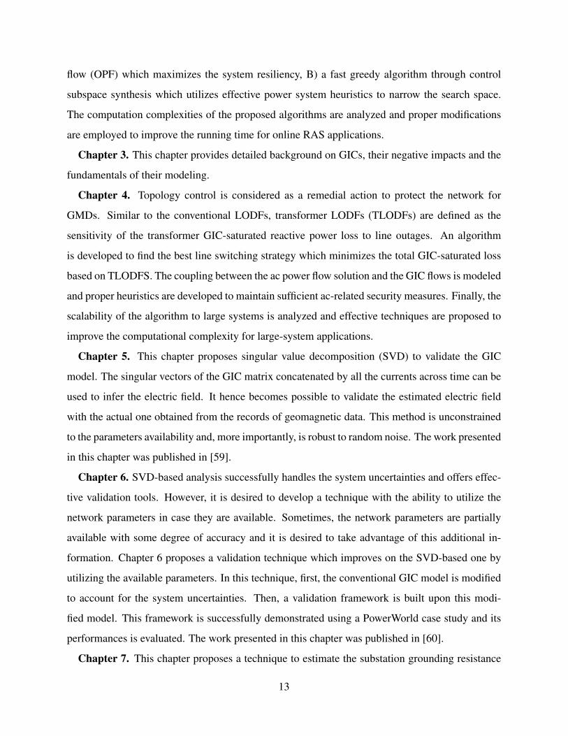
RAS includes a line status monitoring system to detect the contingencies. Controller logic is
designed to evoke the proper action for each contingency as illustrated through an example in Fig.
2.2. In this example, the loss of line A triggers the RAS Action I. The subsequent loss of line B
activates RAS Action II (possibly more severe). The loss of line B by itself will not evoke any
RAS action.
The amount of load/generation that needs to be shed in a RAS action depends on the state of
19
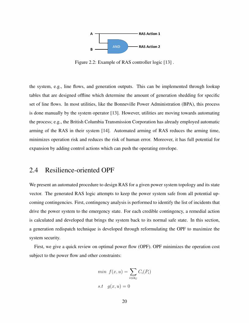
Figure 2.2: Example of RAS controller logic [13] .
the system, e.g., line flows, and generation outputs. This can be implemented through lookup
tables that are designed offline which determine the amount of generation shedding for specific
set of line flows. In most utilities, like the Bonneville Power Administration (BPA), this process
is done manually by the system operator [13]. However, utilities are moving towards automating
the process; e.g., the British Columbia Transmission Corporation has already employed automatic
arming of the RAS in their system [14]. Automated arming of RAS reduces the arming time,
minimizes operation risk and reduces the risk of human error. Moreover, it has full potential for
expansion by adding control actions which can push the operating envelope.
2.4 Resilience-oriented OPF
We present an automated procedure to design RAS for a given power system topology and its state
vector. The generated RAS logic attempts to keep the power system safe from all potential up-
coming contingencies. First, contingency analysis is performed to identify the list of incidents that
drive the power system to the emergency state. For each credible contingency, a remedial action
is calculated and developed that brings the system back to its normal safe state. In this section,
a generation redispatch technique is developed through reformulating the OPF to maximize the
system security.
First, we give a quick review on optimal power flow (OPF). OPF minimizes the operation cost
subject to the power flow and other constraints:
min f(x, u) =∑i∈UG
Ci(Pi)
s.t g(x, u) = 0
20

h(x, u) ≤ 0 (2.1)
where u is the control variable and x is the state variable, which includes the voltage phasors
(magnitudes and phase angles) on individual power buses. The voltage magnitude of the PV buses
(generators) and the voltage magnitude and angle of the slack bus are excluded since their values
are known. The control variables are the generator MW output set-points, settings of the flexible
alternating current transmission system (FACTS) devices, phase shifting transformers, and static
VAR compensators. For simplicity and without loss of generality, only the generator MW output
may be considered as control variable and the objective function may be written as:
f(x, u) =∑i∈UG
Ci(Pi) (2.2)
where Ci(Pi) is the cost of operating generator i with the MW output of Pi, and UG is the set of
generators.
The equality constraint g(x, u) corresponds to the power flow equations and ensures that the
active and reactive power at the PQ buses (loads) and the active power at the PV buses (generators)
match their given values. The inequality constraint h(x, u) may include the line flow limits, the
voltage magnitude limits and the generators output limit as given by:
V mini ≤ Vi ≤ V max
i i ∈ UPQ
Pmini ≤ Pi ≤ Pmax
i i ∈ UPV
Qmini ≤ Qi ≤ Qmax
i i ∈ UPV
Pi,j ≤ Pmaxi,j (i, j) ∈ I (2.3)
where Vi, Pi and Qi are respectively the voltage magnitude, the active power and the reactive
power at bus i; and UPQ and UPV are the set of PQ and PV buses, respectively. Pi,j is the active
power on the line between buses i and j, Pmaxi,j is the flow limit of this line, and I is the set of all
(i, j) for which there is a line connecting bus i to bus j. Note that the generator output limit is a
physical constraint and cannot be violated at any time. On the other hand, the voltage limit and line
flow limits are operating constraints that relate to system reliability, and these may be formulated
21

as soft constraints.
2.4.1 Security Constrained OPF
The first step in SCOPF is to determine the list of contingencies to be considered. The list includes
contingencies which are likely to occur and violate at least one of the network constraints. In-
significant or infrequent contingencies are ignored. SCOPF determines the optimal control which
minimizes the objective function for the base case and satisfies the power flow feasibility and the
network constraints for the base case and each contingency case as expressed in:
min f(x(0), u)
s.tg(j)(x(j), u) = 0
h(j)(x(j), u) ≤ 0
j = 0, 1, · · · , K (2.4)
where x(j), g(j), and h(j) represent the state, the power flow feasibility, and the network constraints
for the contingency case j, respectively. K is the size of the contingency list. The pre-contingency
or base case is denoted by j = 0 as expressed in
j =
0 base case
1 ≤ k ≤ K contingency case k(2.5)
SCOPF ensures that the system remains in the normal state and does not transition to the emer-
gency state when a contingency occurs. It increases the system security and eliminates the need for
remedial action schemes. However, this is achieved with the expense of less economical operation.
The additional constraints for the contingency cases reduce the size of the feasible solution space.
Therefore, the solution from SCOPF has a higher cost than the one from OPF as illustrated in Fig.
2.3.
22
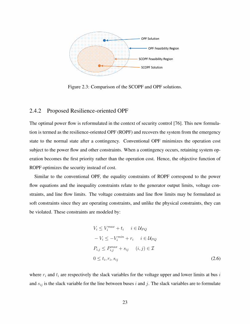
Figure 2.3: Comparison of the SCOPF and OPF solutions.
2.4.2 Proposed Resilience-oriented OPF
The optimal power flow is reformulated in the context of security control [76]. This new formula-
tion is termed as the resilience-oriented OPF (ROPF) and recovers the system from the emergency
state to the normal state after a contingency. Conventional OPF minimizes the operation cost
subject to the power flow and other constraints. When a contingency occurs, retaining system op-
eration becomes the first priority rather than the operation cost. Hence, the objective function of
ROPF optimizes the security instead of cost.
Similar to the conventional OPF, the equality constraints of ROPF correspond to the power
flow equations and the inequality constraints relate to the generator output limits, voltage con-
straints, and line flow limits. The voltage constraints and line flow limits may be formulated as
soft constraints since they are operating constraints, and unlike the physical constraints, they can
be violated. These constraints are modeled by:
Vi ≤ V maxi + ti i ∈ UPQ
− Vi ≤ −V mini + ri i ∈ UPQ
Pi,j ≤ Pmaxi,j + sij (i, j) ∈ I
0 ≤ ti, ri, sij (2.6)
where ri and ti are respectively the slack variables for the voltage upper and lower limits at bus i
and sij is the slack variable for the line between buses i and j. The slack variables are to formulate
23

the soft constraints and are penalized in the objective function. The objective function enforces the
voltage constraints and the line flow limits as expressed in:
f(x) =∑i∈UPQ
VV (2ti + t2i ) +∑i∈UPQ
VV(2ri + r2i )
+∑
(i,k)∈I
VI(2sik + s2ik) (2.7)
where VV , VV and VI are the weighting parameters chosen with respect to the desired importance
of each term.
Solving the proposed ROPF is computationally expensive and might not be practical for a larger
system. In the case of a credible contingency, it is crucial to take an effective control action
as quickly as possible. Hence, finding a solution that is less accurate, but faster to compute is
preferable. Motivated by this, the optimization problem is simplified to reduce the computational
complexity. First, the equality constraints associated with the power flow equations are linearized
and similar to DC-OPF, DC-ROPF is defined [77]. Second, the inequality constraints associated
with the voltage limit are relaxed. The objective function is modified accordingly to exclude the
terms associated with the voltage limits:
f(x) =∑
(i,j)∈I
(2sij + s2ij)−∑i∈N
ui (2.8a)
s.t : Pmini ≤ Pi ≤ Pmax
i i ∈ UPV (2.8b)
Qmini ≤ Qi ≤ Qmax
i i ∈ UPV (2.8c)
Bij(θi − θj) = Pij (i, j) ∈ I (2.8d)∑(i,j)∈I
Pij −∑
(j,i)∈I
Pji + Pi −Di + ui = 0 i ∈ N (2.8e)
0 ≤ ui ≤ Di i ∈ N (2.8f)
Pij ≤ Pmaxij + sij (i, j) ∈ I (2.8g)
0 ≤ sij (2.8h)
where Di is the demand at bus i. Constraint (2.8e) relaxes the node balance constraint by allowing
24
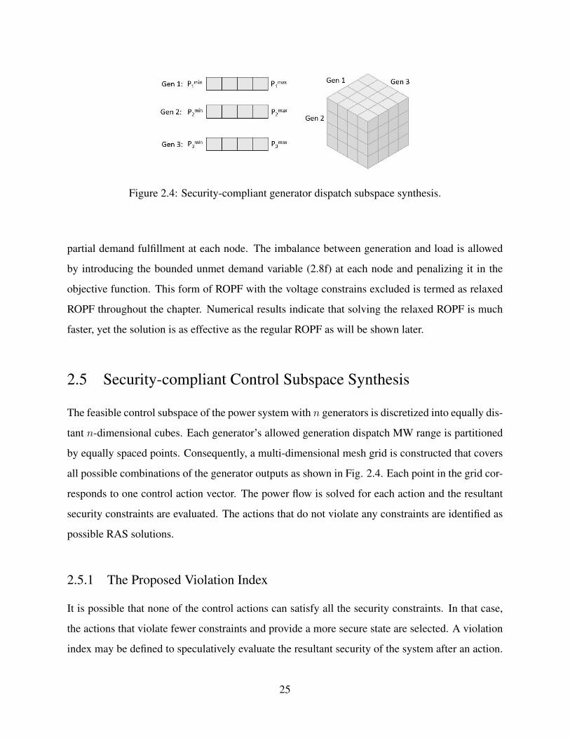
Figure 2.4: Security-compliant generator dispatch subspace synthesis.
partial demand fulfillment at each node. The imbalance between generation and load is allowed
by introducing the bounded unmet demand variable (2.8f) at each node and penalizing it in the
objective function. This form of ROPF with the voltage constrains excluded is termed as relaxed
ROPF throughout the chapter. Numerical results indicate that solving the relaxed ROPF is much
faster, yet the solution is as effective as the regular ROPF as will be shown later.
2.5 Security-compliant Control Subspace Synthesis
The feasible control subspace of the power system with n generators is discretized into equally dis-
tant n-dimensional cubes. Each generator’s allowed generation dispatch MW range is partitioned
by equally spaced points. Consequently, a multi-dimensional mesh grid is constructed that covers
all possible combinations of the generator outputs as shown in Fig. 2.4. Each point in the grid cor-
responds to one control action vector. The power flow is solved for each action and the resultant
security constraints are evaluated. The actions that do not violate any constraints are identified as
possible RAS solutions.
2.5.1 The Proposed Violation Index
It is possible that none of the control actions can satisfy all the security constraints. In that case,
the actions that violate fewer constraints and provide a more secure state are selected. A violation
index may be defined to speculatively evaluate the resultant security of the system after an action.
25

Aggregate MVA overload (AMWCO) is introduced in [78] which evaluates the system security
based on the total amount of current flow violations,
AMWCO =∑
(i,j)∈I
max0, P (k)ij − Pmax
ij (2.9)
This security index considers only the line flow violations, and excludes the bus voltage or the
generator power limits. A security index is defined to account for these constraints,
V iolation(k) =wIS(k)I + wV S
(k)V + wPS
(k)P + wQS
(k)Q (2.10)
where S(k)I , S(k)
V , S(k)P , and S(k)
Q are respectively the security indices of the line flows, bus voltages,
generator active power and reactive power for action k. The terms wI , wV , wP and wQ are their
corresponding weights which capture varying importance of different violation type. The security
index for the line flows is given by
S(k)I =
∑(i,j)∈I
max0, P (k)ij − Pmax
ij Pmaxij
(2.11)
This is similar to the aggregate MVA overload in (2.9) except that the MVA overloads are normal-
ized by the line flow limits. The violation index for bus voltage, and generator limits are defined
similarly as the aggregate violations normalized by their upper bound limits.
The importance of using the normalization terms and the weightsw can be demonstrated through
an example. Consider two constraint violations: The first violation is on a bus with voltage of
Vi = 1.5 p.u. and maximum permissible voltage of V maxi = 1.05 p.u. The second violation is
on a line with Pjk = 800 MW active power which has a MW limit of Pmaxjk = 400 MW. The
amount of violation is (Vi − V maxi ) = 0.45 and Pjk − Pmax
jk = 400 for the second one. The first
violation is more severe than the second one, yet its amount is much smaller. Normalizing the
violation amount by its upper bound limit results in 0.43 for the first violation and 1 for the second
one. The violation of voltage constraint is more significant than line flow constraint violation of
the same percentage. Hence, higher weight is assigned to the voltage constraint in order to capture
its significance. Considering the weights of wV = 1 and wI = 0.05 results in 0.43 for the first
26

violation and 0.05 for the second one. Now, the terms corresponding to each constraint which
appear in the violation index reflect their actual importance to the system security. The current
framework considers a rather heuristic approach for assigning the proper weights. Developing a
systematic approach for calculating the weights will be an interesting future study.
2.5.2 The Performance Improvements
The computational complexity of the control subspace synthesis algorithm is O(Rn), where R
is the discretization granularity for the individual generators, n is the number of generators that
can participate in the dispatch, and O() is the big O time complexity notation. The complexity is
exponential in the number of participating generators. For a large system with many generators,
the exponential time complexity will be burdensome or even impossible. One approach is to
reduce the number of participating generators. Individual generators may have varying impact on
the overall system security with some generators being crucial and others being less significant.
Excluding less significant generators from the search reduces the number of safe/safer actions
considered, while still providing enough candidates to keep the performance near optimal. This
will be demonstrated through case studies later in this chapter.
We employ a greedy algorithm to identify the insignificant set of generators to be excluded from
the search procedure. For every contingency, the lines and buses at which the constraints are vi-
olated are identified. Based on empirical analyses, we observe the identified lines and buses are
often clustered at one or multiple locations in the network. The generators close to the areas under
stress are classified as crucial and the ones which are further away are labeled as insignificant. The
most critical generators are determined in the first level of the algorithm. The less critical gener-
ators are determined in subsequent levels of the algorithm. The levels are executed consecutively
until the number of critical generators reaches a user-specified value. Algorithm 1 describes more
precisely how our framework identifies the critical generators with varying level of importance. In
the Algorithm, UkCritbus and UkCritbus are respectively the set of critical buses and critical generators
at level k, CritGenMax is the maximum number of critical generators defined by the user and
Size(x) returns the size of the set x.
We demonstrate the effectiveness of this technique on case studies later in this chapter. While
27

Algorithm 1 Critical Generator Identification (CGI)1: procedure CGI(Network State and Limits)2: U1
Critbus = Set of busses with Violations3: U1
Critgen = UPV ∩ U1Critbus
4: k = 15: while Size(UkCritgen) < CritgenMax do6: UkCritbus = Uk−1Critbus ∪N(Uk−1Critbus)7: UkCritGen = Uk−1CritGen ∪ (UPV ∩ UkCritbus)8: k = k + 19: end while
10: end procedure
this is a heuristic technique, it gives very promising results based on our experimentation. We
consider development of a systematic and efficient approach with theoretical guarantees to identify
the truly-optimal set of crucial generators as a future study.
A second approach for reducing the computational complexity is to exclude some of the non-
promising candidates based on the power losses in the system. For each candidate generation
dispatch, the total load is fixed, the real output power of all the generators except for the slack bus
is known and the real power at the slack generator is limited by its output power bounds. Motivated
by this, the mismatch between the total generation and load may be used as a criteria to reduce the
size of the search space:
Pminslack − δ ≤ (PLoad −
∑i∈UPV
Pi) ' Pslack ≤ Pmaxslack + δ (2.12)
where PLoad is the total load in the system, Pslack is the MW output of the slack generator, Pmaxslack
and Pminslack are respectively the upper and lower bounds of the slack generator’s MW output and δ is
the margin of error. The control subspace synthesis with all the combinations for all the generators
is referred to as full exhaustive search and the one with only the critical generators and the system
loss filtering is termed as the selective search throughout the chapter.
The computation time can be further reduced through using DCPF instead of AC power flow to
get the system states for each possible action. Since the DCPF solution is not accurate, it could
be used as a fast screening tool before detailed ACPF analysis is performed on the top candidates.
The violation index of all the candidate action is calculated based on their DCPF solutions and the
28

Table 2.1: Comparison of the ROPF Methods for the 24-bus System
Scenario Number of Violations Violation
Gen MW VoltageLineFlow AMWCO
IndexTime(sec)
No Action 0 7 3 2.3507 0.2183 -
ROPF 0 2 0 0 0.021338.11
Relaxed ROPF 0 2 0 0 0.0246 36.87RelaxedDC-ROPF
0 2 1 1.1621 0.02569.1946
top candidates are selected. AC power flow is solved for only the top candidates; the exact value
of their violation indices are obtained and the best action is obtained accordingly.
2.6 Simulation and Numerical Results
The performance of the proposed algorithm is evaluated through simulation. The IEEE 24-bus
system and the IEEE 118-bus [55] are considered, contingencies are applied to these systems, and
effective RAS actions are designed to maintain their security.
First, contingency analysis is performed on the 24-bus system. Figure 2.5 illustrates the number
of violations and the violation index as broken down by type for all the single and double generator
outage contingencies. It is observed that voltage violations contribute the most to the violation
index. The generator outage at bus 23 has the highest violation index among all the single outages
and hence is selected as the most credible one for further analysis. The power flow is solved for
this contingency case and the security constraints are evaluated. It is observed that this contingency
violates seven voltage constraints and three line flow constraints. The violation index of the system
prior to any control action is 0.2181 as calculated by (2.10). The assumed weights for the violation
index are wV = 1, wP = wQ = 100 and wI = 0.05. This selection captures the lower sensitivity of
the system security to the percentage violation of line flow limits compared to voltage constraints.
The motivation for using high weights for the generator limits is that satisfying physical constraints
is more important than satisfying operating constraints.
29
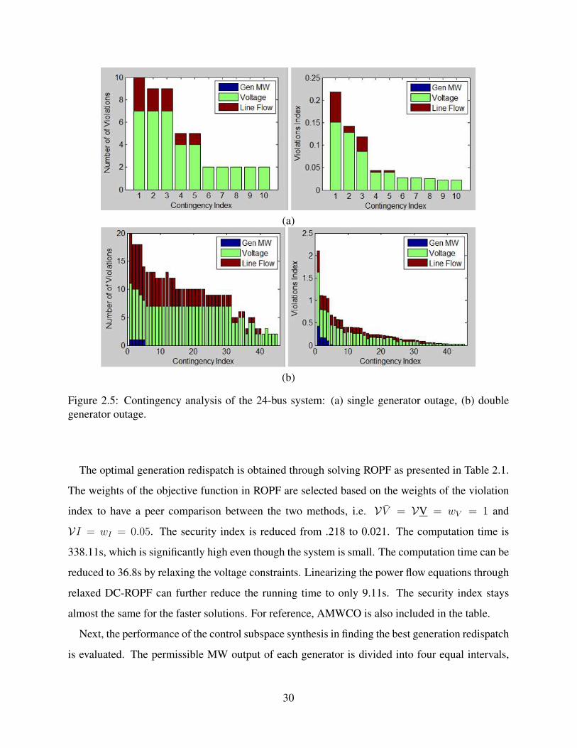
(a)
(b)
Figure 2.5: Contingency analysis of the 24-bus system: (a) single generator outage, (b) doublegenerator outage.
The optimal generation redispatch is obtained through solving ROPF as presented in Table 2.1.
The weights of the objective function in ROPF are selected based on the weights of the violation
index to have a peer comparison between the two methods, i.e. VV = VV = wV = 1 and
VI = wI = 0.05. The security index is reduced from .218 to 0.021. The computation time is
338.11s, which is significantly high even though the system is small. The computation time can be
reduced to 36.8s by relaxing the voltage constraints. Linearizing the power flow equations through
relaxed DC-ROPF can further reduce the running time to only 9.11s. The security index stays
almost the same for the faster solutions. For reference, AMWCO is also included in the table.
Next, the performance of the control subspace synthesis in finding the best generation redispatch
is evaluated. The permissible MW output of each generator is divided into four equal intervals,
30
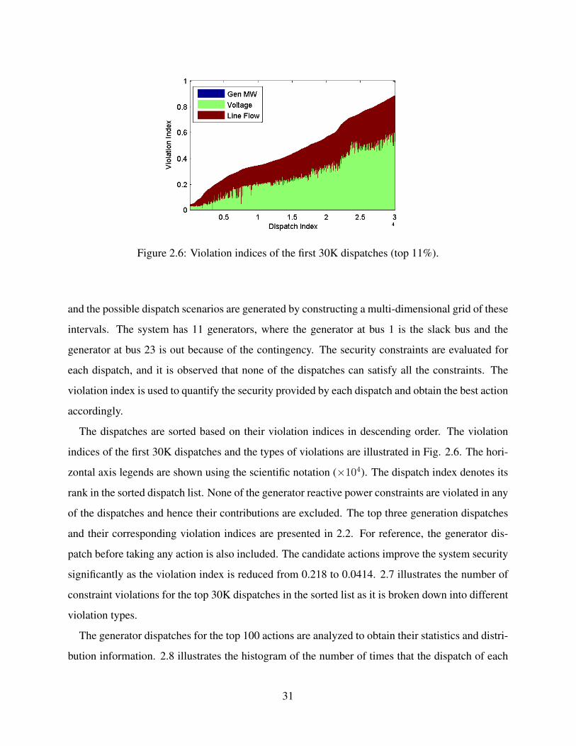
Figure 2.6: Violation indices of the first 30K dispatches (top 11%).
and the possible dispatch scenarios are generated by constructing a multi-dimensional grid of these
intervals. The system has 11 generators, where the generator at bus 1 is the slack bus and the
generator at bus 23 is out because of the contingency. The security constraints are evaluated for
each dispatch, and it is observed that none of the dispatches can satisfy all the constraints. The
violation index is used to quantify the security provided by each dispatch and obtain the best action
accordingly.
The dispatches are sorted based on their violation indices in descending order. The violation
indices of the first 30K dispatches and the types of violations are illustrated in Fig. 2.6. The hori-
zontal axis legends are shown using the scientific notation (×104). The dispatch index denotes its
rank in the sorted dispatch list. None of the generator reactive power constraints are violated in any
of the dispatches and hence their contributions are excluded. The top three generation dispatches
and their corresponding violation indices are presented in 2.2. For reference, the generator dis-
patch before taking any action is also included. The candidate actions improve the system security
significantly as the violation index is reduced from 0.218 to 0.0414. 2.7 illustrates the number of
constraint violations for the top 30K dispatches in the sorted list as it is broken down into different
violation types.
The generator dispatches for the top 100 actions are analyzed to obtain their statistics and distri-
bution information. 2.8 illustrates the histogram of the number of times that the dispatch of each
31

Table 2.2: Top Three Dispatches by the Exhaustive Search
GenNumber
No ActionGeneration Redispatch
Action 1 Action 2 Action 31 0.3637 1.06 1.07 1.072 1.37 3.33 3.33 3.337 2.72 3.33 3.33 3.33
13 4.64 6.67 6.67 6.6714 0 3.33 3.33 3.3315 1.4 3.33 3.33 6.6716 1.4 3.33 0.00 0.0018 3.63 0.00 3.33 3.3321 3.63 3.33 3.33 0.0022 2.72 0.00 0.00 0.00
ViolationIndex 0.2183 0.0414 0.0416 0.0417
Table 2.3: Critical Generator Identification (CGI)
CGI Level Critical GeneratorsLevel 1 2Level 2 7Level 3 13,14,15Insignificant Generators 16,18,21,22
generator was in any of the intervals. We observe that the dispatch of some generators is always
within only one or two intervals; e.g., Gen 2 dispatch is always at the first and second interval and
Gen 7 dispatch is mostly at the second interval. In contrast, the dispatch of some generators like
Gen 16, Gen 18, Gen 21 and Gen 22 falls within all intervals. This suggests that the dispatches of
these generators are relatively insignificant to the system security and could be excluded from the
exhaustive search for faster computation, as discussed below.
The computation time may be reduced by narrowing down the search space through selective
search. The critical generators are identified using the proposed algorithm (Table 2.3). The most
critical generators are Gen 2 and Gen 7 that are identified in the first and second levels of the
algorithm, while Gen 13, Gen 14, and Gen 15 are identified as third order critical generators. The
32

Figure 2.7: Number of violations for the first 30K dispatches (top 11%).
remaining generators, Gen 18, 21, 22, and 23, are labeled as insignificant.
Figure 2.9 shows the line flows and the voltage profile of the system after the contingency. The
line flows are visualized through the pie charts on the lines and the voltage profile through the
contour plot. The figure shows the stressed area, where the overloaded lines and under voltage
buses are located. Gen 2 and Gen 7 are the closest to the stressed area as correctly identified in
the first and second level of Critical Generator Identification (CGI); Gen 13, Gen 14 and Gen 15
are in the second order neighborhood, and the remaining generators are far enough to be excluded
from the exhaustive search. These results are consistent with the earlier observation of the dispatch
distributions from Fig. 2.8. The dispatch of the critical generators among the top 100 actions is
within only a few intervals, whereas the dispatch of the insignificant ones is distributed between
all the intervals.
Once the critical generators are determined, the MW outputs of the four insignificant generators
are fixed to their default values and the selective search is performed on the five critical generators.
This reduces the number of combinations significantly, i.e., 49/45 = 256 times. The number of
combinations can be further decreased by considering the mismatch between the total load and
generation for each action and excluding the non-promising ones. The 45 = 1024 combinations
from the critical generators are sorted based on their violation index in descending order. The
mismatch between the total generators MW output (excluding the slack generator) and the total
33

1 2 3 4
50100
Gen
2
1 2 3 4
50100
Gen
71 2 3 4
50100
Gen
13
1 2 3 4
50100
Gen
14
1 2 3 4
50100
Gen
15
1 2 3 4
50100
Gen
16
1 2 3 4
50100
Gen
18
1 2 3 4
50100
Gen
21
1 2 3 4
50100
Gen
22
interval number
Figure 2.8: Distribution of the generators’ dispatches among the top 100 actions. The dispatch ofthe critical generators is within only a few intervals, whereas the dispatch of the insignificant onesis distributed between all the intervals.
load for the first 800 dispatches in the sorted list are illustrated in Fig. 2.10. The mismatch falls
within the range specified by (2.12) for the top 27% candidates (first 178 dispatches). Hence, using
the load/generation mismatch as a criteria to eliminate non-promising candidates can reduce the
number of candidates by an extra 70% without compromising the performance.
The performance of the selective search relies on the correct identification of the critical gener-
ators. To demonstrate this, the participating generators are selected randomly as opposed to using
the CGI algorithm. Table 2.4 presents the comparison between different control subspace methods.
Five scenarios are considered:
34

Figure 2.9: Visualization of the constraint violations for the 24-bus system: The pie charts visualizethe line flows with red denoting violations. The contour plot visualizes the voltage profile with theblue areas illustrating violations.
1. Full Search: All the possible combination of generation redispatches are considered.
2. Selective Search: Only the critical generators are included and the search is narrowed based
on the system losses.
3. Naive Search: The generators that participate in RAS are selected randomly and the search
is narrowed based on the system losses.
4. Selective search with DCPF: DCPF is used in the selective search for solving power flow
5. Naive search with DCPF: DCPF is used in the naive search for solving power flow.
The running time of the full search is extremely high (10085s), which makes it impractical for
online RAS applications. The selective search provides the same performance as the full search
with much lower computation time (only 0.09% of the full search running time). The violation
index obtained from the naïve search is much higher than the smart search, which validates the
35
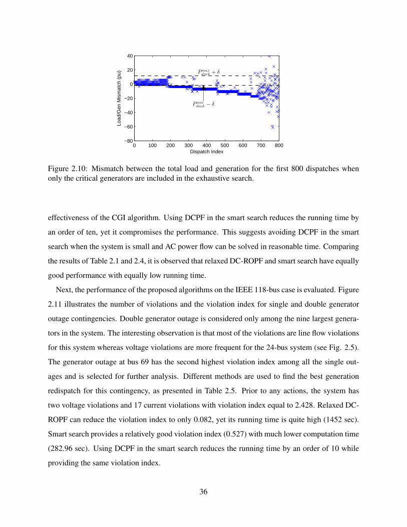
0 100 200 300 400 500 600 700 800−80
−60
−40
−20
0
20
40
Pmax
slack+ δ
Dispatch Index
Load
/Gen
Mis
mat
ch (
pu)
Pmin
slack− δ
Figure 2.10: Mismatch between the total load and generation for the first 800 dispatches whenonly the critical generators are included in the exhaustive search.
effectiveness of the CGI algorithm. Using DCPF in the smart search reduces the running time by
an order of ten, yet it compromises the performance. This suggests avoiding DCPF in the smart
search when the system is small and AC power flow can be solved in reasonable time. Comparing
the results of Table 2.1 and 2.4, it is observed that relaxed DC-ROPF and smart search have equally
good performance with equally low running time.
Next, the performance of the proposed algorithms on the IEEE 118-bus case is evaluated. Figure
2.11 illustrates the number of violations and the violation index for single and double generator
outage contingencies. Double generator outage is considered only among the nine largest genera-
tors in the system. The interesting observation is that most of the violations are line flow violations
for this system whereas voltage violations are more frequent for the 24-bus system (see Fig. 2.5).
The generator outage at bus 69 has the second highest violation index among all the single out-
ages and is selected for further analysis. Different methods are used to find the best generation
redispatch for this contingency, as presented in Table 2.5. Prior to any actions, the system has
two voltage violations and 17 current violations with violation index equal to 2.428. Relaxed DC-
ROPF can reduce the violation index to only 0.082, yet its running time is quite high (1452 sec).
Smart search provides a relatively good violation index (0.527) with much lower computation time
(282.96 sec). Using DCPF in the smart search reduces the running time by an order of 10 while
providing the same violation index.
36

Table 2.4: Comparison of the Control Subspace Synthesis Methods for the 24 bus System
Scenario Number of Violations ViolationGenMW
VoltageLineFlow
AMWCO IndexTime(sec)
No Action 0 7 3 2.3507 0.2183 -
Full Search 0 3 1 0.3812 0.041410085
Smart Search 0 5 2 0.5486 0.058 9.44Smart Searchwith DCPF
0 6 1 0.3944 0.1284 0.934
Naive Search 1 10 7 0.5486 5.0494 12.8Naive Searchwith DCPF
1 8 2 0.5032 5.9680.9212
Recall that using DCPF for the 24 bus system compromised the violation index. Linearizing the
power flow equations through DCPF has varying impact on different systems depending on how
inductive the transmission lines are, the system voltage profile, etc. The effect of using DCPF on
the smart search performance depends on similar characteristics of the system. It also depends on
the type of post-contingency violations. For example, if the post-contingency violations are mostly
line flow violations (e.g. the 118bus system), using DCPF in the smart search would be effective
since DCPF captures the coupling between the generation redispatch and the line flows. On the
other hand, if the violations are mostly voltage violations (e.g. the 24-bus case), using DCPF in
the smart search jeopardizes the performance since there is no coupling between the voltages and
the generator MW outputs in DCPF. Further exploration into the application of DCPF in the smart
search and its effect on the performance will be an interesting future study.
All the credible single generator outages are considered for the 118-bus system, and the smart
search with DCPF is used to improve the system security. In this study, a contingency is considered
credible when the post-contingency violation index exceeds 0.1. The violation index before taking
any action is compared with the one from the smart search in Fig. 2.12. It is observed that the
smart search successfully protects the network from all the credible contingencies.
The last system to study is the Texas 2000-bus synthetic case with the one-line diagram shown
in Fig. 2.13 [55, 79]. The system has eight geographic areas which are color-coded in the one-line
37

(a)
(b)
Figure 2.11: Contingency analysis for the 118-bus system: (a) single generator outage, (b) doublegenerator outage.
diagram; red lines are 345 kV and black lines are 115 kV. Figure 2.14 illustrates the number of
violations and violation index for the single and double generator outages. The single outage is
performed only on the first 24 largest generators and the double outage only among the first seven
largest generators. Gen MW contributes the most to the violation index for this system, unlike
the 24-bus and the 118-bus which had voltage violations and line flow violations as the dominant
violation type, respectively. All the single generator outages for this system have very low violation
index (smaller than 0.8). Hence, the most credible double generator outage is selected for further
analysis, i.e. generator outages at buses 1593 and 1735. Table 2.6 presents the performance of
the smart search with DCPF in finding the best generation redispatch. Prior to any action, the
violation index is 4.7 with three generator MW violations, 94 voltage violations and 22 line flow
38

Table 2.5: Method Comparison for the 118-bus System
Scenario Number of Violations ViolationGenMW
VoltageLineFlow AMWCO
IndexTime(sec)
No Action 0 2 17 9.79 2.428 -RelaxedDC-ROPF
8 1 0 0 0.0825 1452
Smart Search 0 3 12 0.0403 0.5274 282.96Smart Searchwith DCPF
0 3 12 2.066 0.527 28.59
Naive Searchwith DCPF
1 1 3 4.246 193.9
Table 2.6: Generation Redispatch for the 2000-bus System
Scenario Number of Violations ViolationGenMW
VoltageLineFlow
IndexTime(sec)
No Action 3 94 22 4.70 -Smart Search with DCPF 2 2 1 0.63 242.9
violations. The generation redispatch reduces the violation index to 0.63 with only two Gen MW
violations, two voltage violations, and one line flow violation. The algorithm considers eight
critical generators with five intervals for each generator. It is important to use DCPF for this
system instead of ACPF due to its large size. The running time of solving ACPF is 5.05 seconds
while the DCPF running time is only 0.067. The performance of ROPF is not tested on this system
because of its computational complexity limitations.
2.7 Conclusion
In this chapter, we developed a design procedure for remedial action schemes (RAS) which im-
proves the security of the power system against credible contingencies. Resilience-oriented OPF
and security-compliant control subspace synthesis are proposed as two generation redispatch tech-
39

0 2 4 6 8 10 12 140
1
2
3
4
5
Credible Generator Outage ID
Vio
latio
n In
dex
No Action
Selective Search RAS
Figure 2.12: Performance of the smart search with DCPF in improving the system security duringthe credible generator outages of the 118 bus system.
niques that have low computational complexity and are suitable for online RAS applications. Nu-
merical results on the small IEEE 24-bus test case indicate that both methods provide sufficient
security for the system with reasonable running time. For a larger case like the IEEE 118-bus
system, ROPF offers extremely good security, yet the running time is quite high for online appli-
cations. On the other hand, the greedy algorithm offers a solution that is less secure, but much
faster to compute. This chapter addresses the trade-off between the security and the computational
complexity of the generation redispatch techniques and allows the system operator to select the
best technique based on the size of the system, the required security measures, and etc.
The chapter suggests several opportunities for future research. First, the proposed control sub-
space synthesis focuses on the generation redispatch as the control action. Future research can
extend this framework to other control actions such as topology control. Second, the algorithm for
critical generators identification may be further improved through controllability analysis and the
use of control support groups identified via sensitivity analysis and clustering techniques.
40
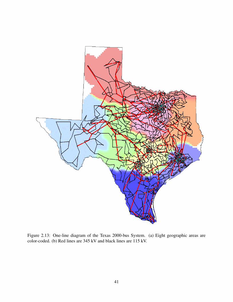
Figure 2.13: One-line diagram of the Texas 2000-bus System. (a) Eight geographic areas arecolor-coded. (b) Red lines are 345 kV and black lines are 115 kV.
41
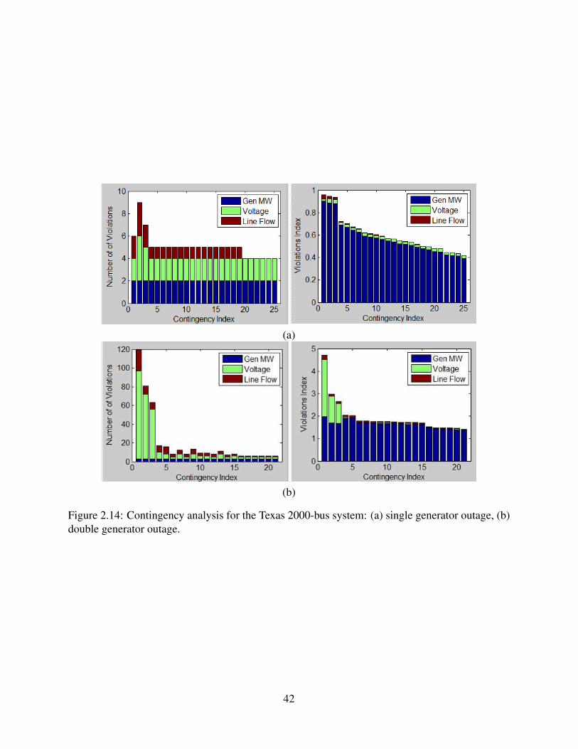
(a)
(b)
Figure 2.14: Contingency analysis for the Texas 2000-bus system: (a) single generator outage, (b)double generator outage.
42
CHAPTER 3
BACKGROUND ON GMD MODELING
This chapter provides detailed background on GICs, their negative impacts and the fundamentals
of their modeling. The chapter is organized as follows: Section 3.1 provides some background on
GMDs. A linear model is presented in Section 3.2 which relates the GICs on transformer neutrals
to E-field through network topology and conductances. In Section 3.3, the relation between the
magnetic field and the E-field is fully described and the estimation of E-field from the magnetic
data is presented. Section 3.4 explains how to estimate the electric field from the GIC measure-
ments.
3.1 Background on Geomagnetic Disturbances
The GICs passing through transformer windings create DC flux in the core of power transformers
which shifts the operating point of their magnetizing characteristics. With the DC offset, the
magnetic flux reaches the saturation level during half of the 60-Hz cycle and the magnetizing
current increases dramatically as shown in Fig. 3.1. This phenomenon is usually referred to as
half-cycle saturation and happens very frequently during GMD events [21, 36].
Half-cycle saturation increases the transformer reactive power loss significantly. Unless suffi-
cient reactive power support is provided to compensate for these losses, the lack of reactive power
in the network may lead to voltage instability and possibly system collapse [37, 80, 33].
Half-cycle saturation increases harmonic currents which in turn increase the eddy current loss
and core loss in some components, e.g. transformers and generators. The additional loss re-
sults in their heating and may cause major damages. Moreover, harmonic currents can affect the
performance of the protection systems. Many of the conventional protection devices such as the
electromechanical relays are sensitive to the current harmonics and are susceptible to misoperation
43
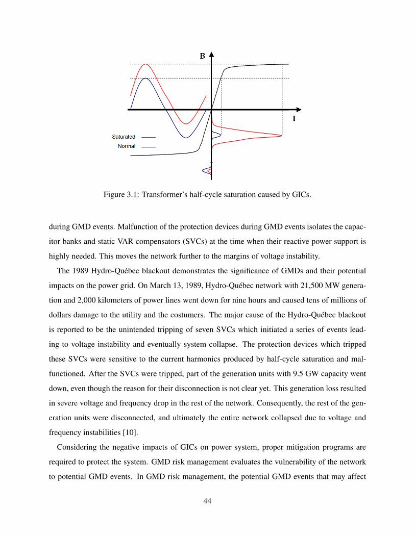
Figure 3.1: Transformer’s half-cycle saturation caused by GICs.
during GMD events. Malfunction of the protection devices during GMD events isolates the capac-
itor banks and static VAR compensators (SVCs) at the time when their reactive power support is
highly needed. This moves the network further to the margins of voltage instability.
The 1989 Hydro-Québec blackout demonstrates the significance of GMDs and their potential
impacts on the power grid. On March 13, 1989, Hydro-Québec network with 21,500 MW genera-
tion and 2,000 kilometers of power lines went down for nine hours and caused tens of millions of
dollars damage to the utility and the costumers. The major cause of the Hydro-Québec blackout
is reported to be the unintended tripping of seven SVCs which initiated a series of events lead-
ing to voltage instability and eventually system collapse. The protection devices which tripped
these SVCs were sensitive to the current harmonics produced by half-cycle saturation and mal-
functioned. After the SVCs were tripped, part of the generation units with 9.5 GW capacity went
down, even though the reason for their disconnection is not clear yet. This generation loss resulted
in severe voltage and frequency drop in the rest of the network. Consequently, the rest of the gen-
eration units were disconnected, and ultimately the entire network collapsed due to voltage and
frequency instabilities [10].
Considering the negative impacts of GICs on power system, proper mitigation programs are
required to protect the system. GMD risk management evaluates the vulnerability of the network
to potential GMD events. In GMD risk management, the potential GMD events that may affect
44
the network are studied and the probabilities of their occurrence are considered. For each potential
GMD, the impacts on the power system are assessed and the potential damages and costs are
estimated. Finally, effective operating procedures are developed which minimize the storm impacts
as well as the mitigation costs.
Reducing the GICs through GIC blocking devices is also an important part of the GIC mitigation
program. Neutral current blocking devices are the neutral resistors or capacitors which are placed
at the neutral-to-ground connection of the transformers. These devices reduce the GIC passing
through the transformer by increasing the resistance of the GIC loop. Series capacitors are also
considered as GIC blocking devices although their main purpose is system stability rather than
GIC reduction. Note that the placement of GIC blocking devices is a very challenging task and
requires careful study on the network topology and equipment configuration. Improper placement
of the blocking devices may block the GIC in one line and direct it to some other line which is
already under stress by GICs.
3.2 GIC Modeling
Within the footprint of an interconnected power system, the geoelectric field is often assumed to
be uniform as represented by E := [EN , EE]T , with EN and EE denoting its Northward and
Eastward components, respectively.
To this end, consider a transmission network with the set of busesNB and the set of substations
N S , which together form the set of nodes N := 1, . . . , N = NB⋃N S . As all the generators
are grounded via the nearest substation, the buses directly connected to generators can be excluded
from NB in the GIC modeling. Furthermore, the node connectivity can be represented by the set
of edges E := (n,m) ⊆ N ×N , which includes the set of transmission lines L := (n,m) ⊆
NB×NB, as well as the pairs (n,m) if and only if substation n is directly connected to busm by a
transformer. For any (n,m) ∈ E , let gnm = gmn denote the equivalent conductance between n and
m, which will be the transmission line conductance if (n,m) ∈ L. Otherwise if n ∈ N S and m ∈
NB, gnm corresponds to the conductance due to transformer windings to the substation neutral
and autotransformers’ series and common windings. Similarly, let gnn represent the grounding
45

conductance of the substation neutral for n ∈ N S . Notice all the conductance quantities have
accounted for the three phases in parallel. With these notations, an N ×N real symmetric matrix
G can be constructed with nonzeros only at its diagonal and entries corresponding to E , with the
(n,m)-th entry given by
Gnm :=
−gnm, if (n,m) ∈ E∑ν∈Nn
gnν , if n = m ∈ NB
gnn +∑
ν∈Nngnν , if n = m ∈ N S
0, otherwise.
(3.1)
The conductance matrix G serves as the counterpart of the bus admittance matrix for ac power
network analysis, as detailed soon.
3.2.1 Input Voltages as Current Injections
The input of GIC modeling is the aforementioned induced voltage along the transmission lines.
The effect of geoelectric field on the line (n,m) ∈ L is equivalent to having a dc voltage source in
series with that line, with the voltage level given by
Unm = ENLNnm + EELEnm (3.2)
where LNnm and LEnm denote the northward and eastward distance for line (n,m). Using the Norton
equivalent, all the induced voltage sources can be converted to dc current injection to every bus n,
as given by
In =∑
(n,m)∈L
Inm =∑
(n,m)∈L
(LNnmgnmE
N + LEnmgnmEE)
(3.3)
I injn =∑(n,m)
I injnm =∑(n,m)
gnmUnm = (∑
(n,m)∈L
LNnmgnm)EN + (∑
(n,m)∈L
LEnmgnm)EE (3.4)
46
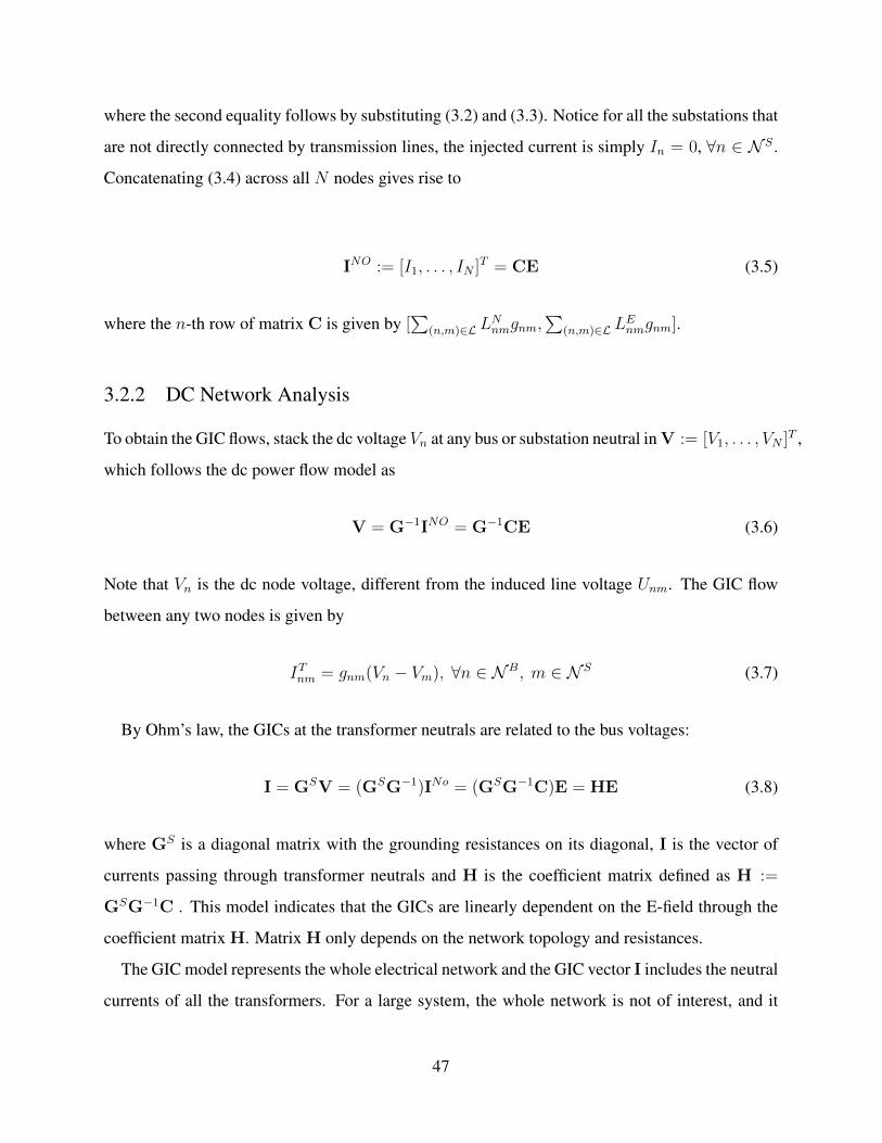
where the second equality follows by substituting (3.2) and (3.3). Notice for all the substations that
are not directly connected by transmission lines, the injected current is simply In = 0, ∀n ∈ N S .
Concatenating (3.4) across all N nodes gives rise to
INO := [I1, . . . , IN ]T = CE (3.5)
where the n-th row of matrix C is given by [∑
(n,m)∈L LNnmgnm,
∑(n,m)∈L L
Enmgnm].
3.2.2 DC Network Analysis
To obtain the GIC flows, stack the dc voltage Vn at any bus or substation neutral in V := [V1, . . . , VN ]T ,
which follows the dc power flow model as
V = G−1INO = G−1CE (3.6)
Note that Vn is the dc node voltage, different from the induced line voltage Unm. The GIC flow
between any two nodes is given by
ITnm = gnm(Vn − Vm), ∀n ∈ NB, m ∈ N S (3.7)
By Ohm’s law, the GICs at the transformer neutrals are related to the bus voltages:
I = GSV = (GSG−1)INo = (GSG−1C)E = HE (3.8)
where GS is a diagonal matrix with the grounding resistances on its diagonal, I is the vector of
currents passing through transformer neutrals and H is the coefficient matrix defined as H :=
GSG−1C . This model indicates that the GICs are linearly dependent on the E-field through the
coefficient matrix H. Matrix H only depends on the network topology and resistances.
The GIC model represents the whole electrical network and the GIC vector I includes the neutral
currents of all the transformers. For a large system, the whole network is not of interest, and it
47

Figure 3.2: Geographic location of the investigated magnetic observatories.
is desired to reduce the model to cover only specific transformers. This can be done by selecting
only the corresponding entries in the I matrix and truncating the coefficient matrix accordingly.
3.3 Electric Field Estimation Based on the Magnetic Data
The magnetic observatories operated by USGS and CSWFC provide magnetic measurements at
multiple locations in North America [81]. The locations of these observatories are shown in Fig.
3.2. The electric field induced on the power lines is related to the magnetic flux density through
the Earth’s surface impedance as given by
E(ω) =1
µ0
Z(ω)B(ω) (3.9)
48

Figure 3.3: Estimation of E-field from magnetic field in frequency domain.
where Z is the earth surface impedance and B is magnetic field intensity. Assuming uniform
conductivity for Earth, the Earth surface impedance is obtained by
Z(ω) =
√jωµ0
σ(3.10)
where σ is the Earth conductivity, ω is the frequency and µ0 is the permeability of free space.
The Earth impedance is a function of frequency; therefore, it is easier to conduct the electric field
calculation in the frequency domain. Fourier transform (FT) is used to convert the magnetic field
data from time domain to frequency domain. In frequency domain, magnetic field intensity is
multiplied by the Earth surface impedance to obtain the electric field. The resulting electric field
is in frequency domain and inverse FT may be used to recover the electric field in time domain.
This process is illustrated in Fig. 3.3.
Studies show that the conductivity of the Earth is not uniform and (3.10) provides a naive ap-
proximation of the Earth surface impedance [44]. To have a better approximation, a layered model
for Earth conductivity is considered as shown in Fig. 3.4. The depth and conductivity of each layer
depends on the tectonic structures of the region. The last layer (the innermost layer) is extremely
deep, and its impedance can be calculated through the uniform conductivity model in (3.10). Hav-
ing the impedance of the last layer, the impedance of each layer is obtained recursively based on
the impedance of the layer below it as given by
Zn = Z0
1 +Zn+1 −Z0
Zn+1 −Z0
e−2kndn
1− Zn+1 −Z0
Zn+1 −Z0
e−2kndn(3.11)
where Z0 is the impedance of the innermost layer, dn is the depth on the nth layer and kn is defined
49
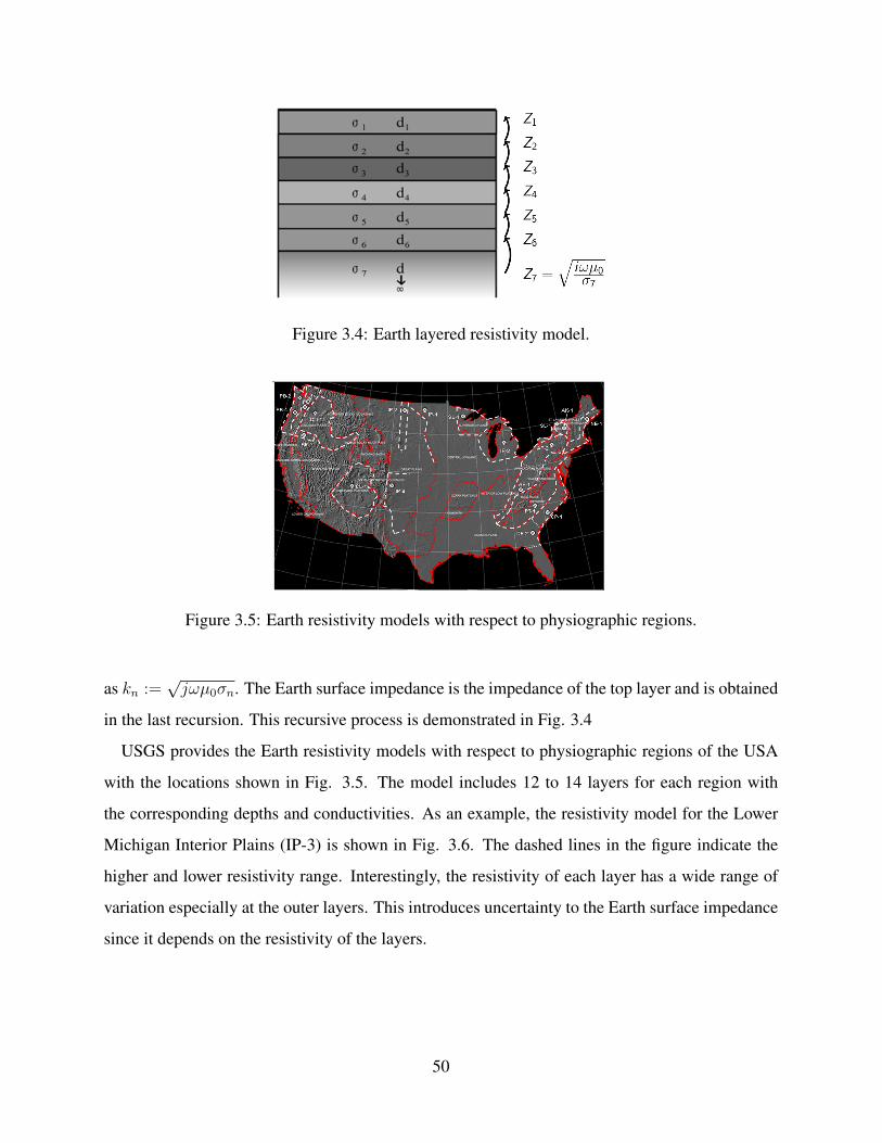
Figure 3.4: Earth layered resistivity model.
Figure 3.5: Earth resistivity models with respect to physiographic regions.
as kn :=√jωµ0σn. The Earth surface impedance is the impedance of the top layer and is obtained
in the last recursion. This recursive process is demonstrated in Fig. 3.4
USGS provides the Earth resistivity models with respect to physiographic regions of the USA
with the locations shown in Fig. 3.5. The model includes 12 to 14 layers for each region with
the corresponding depths and conductivities. As an example, the resistivity model for the Lower
Michigan Interior Plains (IP-3) is shown in Fig. 3.6. The dashed lines in the figure indicate the
higher and lower resistivity range. Interestingly, the resistivity of each layer has a wide range of
variation especially at the outer layers. This introduces uncertainty to the Earth surface impedance
since it depends on the resistivity of the layers.
50

Figure 3.6: Resistivity model for Lower Michigan Interior Plains (IP-3).
3.4 Electric Field Estimation Based on the GIC Data
Assuming a uniform E-field model, at each instant in time, the E-field has two components: the
eastward field EE and the northward field EN . During the GMD, the E-field is dynamic over the
discrete time horizon T := t1, t2, ..., tT, which can be concatenated into the 2× T matrix:
X =
eE,t1eE,t
2. . . eE,t
T
eN,t1eN,t
2. . . eN,t
T
(3.12)
where eE,tn and eN,tn are the eastward and northward E-fields at the nth time instant, respectively.
Similarly, for the dynamic GIC flow I to form the matrix:
Z =
zt
1
1 zt2
1 . . . ztT
1
zt1
2 zt2
2 . . . ztT
2
...... . . . ...
zt1
K zt2
K . . . ztT
K
(3.13)
where ztnk is the GIC reading of the kth sensor at the nth time instant and K is the total number
of sensors. The GIC sensors are installed at the transformers neutral and measure the DC current
51

passing through its neutral. The matrix form of the linear GIC model is given by
Z = HX + V (3.14)
where V is the measurement noise. As the GIC model is linear, the E-field may be obtained from
GIC measurements using various linear estimators. Without prior information of X, the most
popular one is the ordinary LS estimator, as given by
XLS := arg minX‖Z−HZ‖2 = (HTH)−1HTZ (3.15)
where ‖ · ‖2 is the vector Euclidean norm and X is the estimated E-field. Assuming that the
matrix H is full rank, the LS estimator has a simple closed-form solution and thus is efficiently
computable. It is also statistically optimal assuming V is white Gaussian of uniform variance.
If some GIC readings are corrupted outliers, i.e., some entries of V fail to follow the normal
distribution, robust estimation approaches are necessary. A simple one of that kind is the least
absolute value (LAV) estimator, as given by
XLAV := arg minX‖Z−HX‖1 (3.16)
where ‖ · ‖1 denotes the vector Manhattan norm which is equal to the sum of entry-wise absolute
values. Although there is generally no closed-form solution for (10.3), it can be transformed to a
convex linear program, for which efficient solvers are available. The LAV estimator is less accurate
if there are actually no outliers; thus, different robust estimators have been proposed to tackle this,
such as Huber’s Estimator or a more recent one motivated by sparsity [82].
Additional information on X could greatly improve the performance of linear estimators. If the
relative covariance of X with respect to noise standard deviation is known, this gives rise to the
Ridge Regression (RR) by augmenting the LS error criterion as
XRR : = arg minX‖Z−HX‖22 + XT (λI)−1X
52
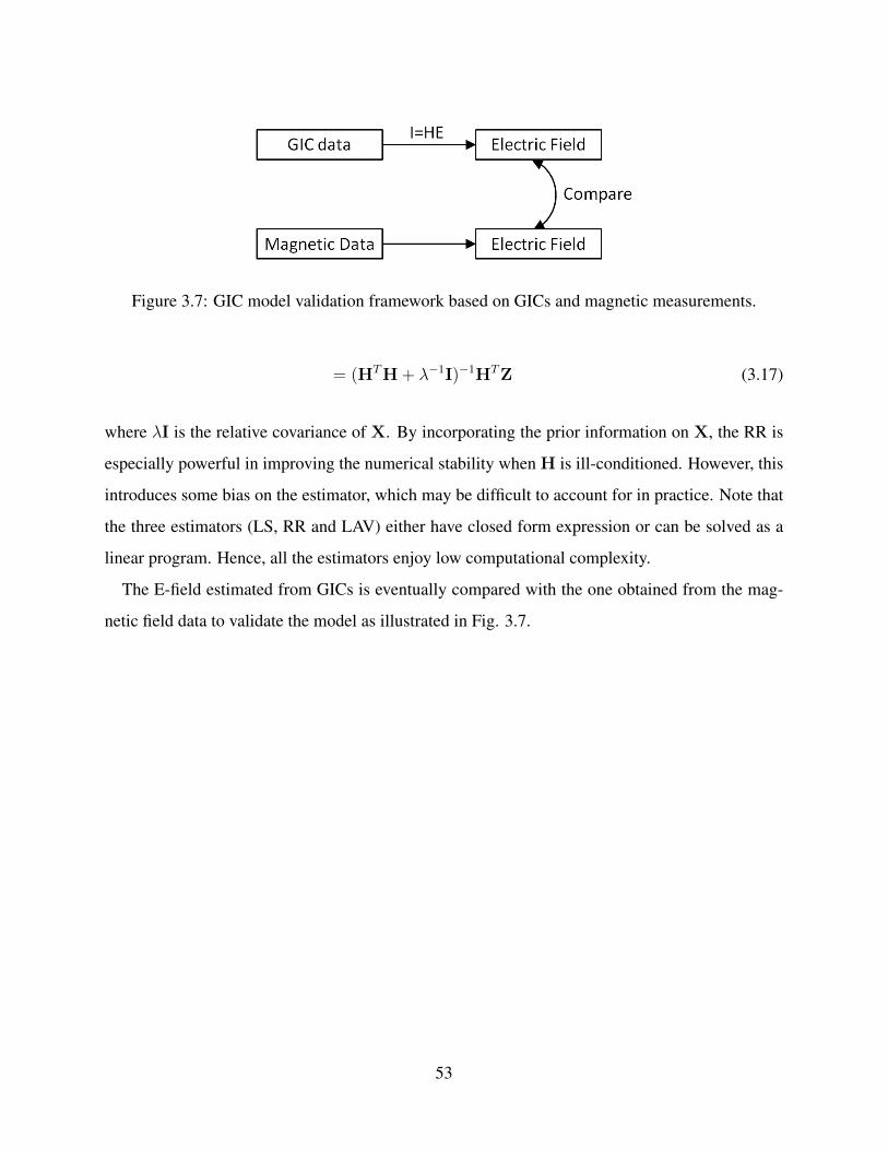
Figure 3.7: GIC model validation framework based on GICs and magnetic measurements.
= (HTH + λ−1I)−1HTZ (3.17)
where λI is the relative covariance of X. By incorporating the prior information on X, the RR is
especially powerful in improving the numerical stability when H is ill-conditioned. However, this
introduces some bias on the estimator, which may be difficult to account for in practice. Note that
the three estimators (LS, RR and LAV) either have closed form expression or can be solved as a
linear program. Hence, all the estimators enjoy low computational complexity.
The E-field estimated from GICs is eventually compared with the one obtained from the mag-
netic field data to validate the model as illustrated in Fig. 3.7.
53
CHAPTER 4
MITIGATION OF GMDS THROUGH LINESWITCHING
4.1 Introduction
Hardening the network against GMDs through corrective control is an effective approach to im-
prove resiliency. This chapter considers line switching as a remedial action for GMD mitigation in
large-scale power systems. The algorithm uses linear sensitivity analysis to find the best switching
strategy which minimizes the GIC-saturated reactive power loss. The coupling between the ac
power flow solution and the GIC flows is modeled and proper heuristics are developed to maintain
sufficient security measures in terms of both GIC flows and ac analysis. Finally, the computational
complexity of the algorithm is analyzed and effective techniques are utilized to reduce its running
time for large-system applications. The effectiveness of the algorithm is demonstrated through
numerical results using a small 20-bus test case as well as large power systems. The algorithm
provides an effective tool to minimize the transformer damage during GMDs and improve the
resiliency.
The chapter is organized as follows: Section 4.2 presents the modeling of GIC-saturated reactive
power loss. Solving power flow including GICs is described in Section 4.3. The proposed line
selection algorithm is presented in Section 4.4. Section 4.5 demonstrates the proposed technique
through numerical results. Section 4.6 presents a conclusion and direction for future work.
54

4.2 Modeling GIC-saturated Reactive Power Loss
The GIC passing through the transformer increases its reactive power loss. GIC-saturated reactive
power loss can be linearly related to the effective GICs as expressed in:
QGIC = KV puIGIC (4.1)
where QGIC is the GIC-saturated reactive power loss, and K is the transformer loss coefficient
which mostly depends on the core type [83]. IGIC is the effective GIC and is calculated based
on the transformer type and winding configuration. For a grounded wye-delta transformer, IGIC
is simply the current in the grounded coil. For transformers with multiple grounded windings (-
autotransformers), the effective current is a function of the current in both coils as expressed in
[84]:
IGIC =aIH + IL
α(4.2)
where IH and IL are respectively the per phase dc current passing through the high side winding
(-series winding) and low side winding (-common winding) and α is the transformer turn ratio.
Calculating IH and IL from (3.7), the effective current at transformer t is given by:
IGICt = gsh(Vh − Vs) +1
αgsl(Vl − Vs) (4.3)
where h and l are the high and low side bus nodes for transformer t, and s is its substation node.
Concatenating (4.3) across all transformers gives rise to:
IGIC = ΦV = ΦG−1CE (4.4)
where Φ is a T × (N +NS) matrix with the (t,m)-th entry given by
55

Φtm :=
gsm, if m = h
αgsm, if m = l
−gsh − αgsl, if m = s
0, otherwise.
(4.5)
4.2.1 Effect of Line Switching on GIC Flows
Next, the effect of opening a line on the GIC flows is studied. Opening line (n,m) modifies the G
matrix by deducting the terms related to the disconnected pairs:
G← G− gnmenmeTnm (4.6)
where vector enm of length N has all zero entries except for the n-th and m-th being +1 and -1,
respectively. Similarly, the H matrix is modified by
H← H− enm[LNnm, LEnm] (4.7)
Opening a line does not affect the Φ matrix. Opening multiple lines requires updating G and H
successively for each opened line.
4.3 Power Flow Solution Including GICs
To solve power flow including the GICs, the GIC-saturated reactive power loss of each transformer
is modeled as a constant current source. Adding these current sources changes the reactive power
injections at the high voltage side of the transformers by:
Qi ← Qi −KV pui IGICi (4.8)
56

where Qi is the reactive power injection at bus i. The power balance equations are nonlinear and
the most common technique for solving them is Newton-Raphson solution. This technique uses
the first order Taylor series to linearize the power balance equations as expressed in: ∆θ
∆|V|
= −J−1
∆P
∆Q
(4.9)
where ∆P (-∆Q) is the vector containing all the real (-reactive) power imbalances and J is Jaco-
bian matrix defined as:
J =
∂∆P
∂∆θ
∂∆P
∂∆|V|∂∆Q
∂∆θ
∂∆Q
∂∆|V|
(4.10)
The algorithm starts with an initial guess, uses (4.9) to update the states in each iteration and
continues the process until the power mismatches are smaller than a threshold. Adding the GIC-
related constant current sources modifies the entries of the Jacobian that correspond to the partial
derivative of the reactive power to voltage magnitudes of the same bus:
∂∆Qi
∂∆|Vi|← ∂∆Qi
∂∆|Vi|−KIGICi (4.11)
The other entries of the Jacobian matrix stay unchanged.
4.4 Iterative Line Switching Algorithm
The transformer LODF (TLODF) can be expressed as:
TLODF = [sij] = [QGIC,(j)i −QGIC,(0)
i ], i ∈ T, j ∈ L (4.12)
where sij is the variation of GIC-saturated loss at transformer i caused by opening line j, QGIC,(j)i
is the GIC-saturated loss at transformer i when line j is opened and QGIC,(0)i is the initial loss. An
analytical technique may be developed to derive TLODFs as a function of the network parameters.
57

Alternatively, one can follow the sensitivity definition to calculate the TLODFs as described in
Algorithm 2. L in the algorithm is the number of lines.
Algorithm 2 Determining the TLODF1: procedure DETERMINING THE TLODF2: Calculate the initial GIC-saturated loss at each transformer, QGIC,(0)
3: for 1 ≤ n ≤ L do4: Open line n5: Calculate the GIC-saturated loss at each transformer, QGIC,(n)
6: Calculate the nth column of the TLODF matrix by QGIC,(n) −QGIC,(0)
7: Close line n8: end for9: end procedure
TLODFs are used to identify the best line switching strategy that minimizes the GIC-saturated
loss. The total loss reduced from opening a line is obtained by taking the sum of TLODF matrix
along the corresponding column. Let QT = Sum(TLODF, 2) be the sum of the TLODF matrix
along the columns. The best lines are obtained by sorting QT in descending order and selecting
the lines with the lowest QT values.
Similar to LODFs, TLODFs consider single line outages. The TLODF for multiple-line outages
is not equal to the sum of the single-line TLODFs of the corresponding lines. The notion of gen-
eralized LODF was introduced in [85] which considers multiple-line LODFs. A similar concept
may be considered for TLODF and analytical techniques can be developed to calculate multiple-
line TLODFs. A rather simple approach for calculating TLODFs under multiple-line outages is
to consecutively open one line and calculate the single-line TLODFs for the new system until all
the desired lines are opened. The line switching algorithm can thus be improved using a similar
approach. First, the TLODF is calculated and the best line to be opened is selected accordingly.
Next, the TLODF matrix is calculated for the new system and the second line to be opened is se-
lected. This process is repeated until the number of opened lines reaches a user-defined threshold,
M . This technique is presented in Algorithm 3.
58

Algorithm 3 Iterative Line Selection1: procedure SELECTING BEST LINES TO OPEN
2: for 1 ≤ m ≤M do3: Calculate TLODFs4: Calculate QT from TLODF5: Find the line with lowest QT and open that line.6: end for7: end procedure
4.4.1 Improving the Computational Complexity
The computational complexity of the proposed algorithm is O(LMT ) where L is the number of
lines, M is the maximum number of lines that can be opened and T is the computation time for
solving for the GIC flows. The number of lines for a power grid is typically slightly larger than the
number of buses. Solving GIC flows requires calculating the inverse of G and then multiplying it
by Φ. G is a sparse matrix roughly in the order of O(N2) and the computation time of taking its
inverse is O(N2.2) [86]. Φ is a sparse matrix of roughly the same order and multiplying it by G−1
requires O(N2+O(1)) [87].
To reduce the running time, first, the TLODF matrix is calculated and QT is calculated for each
line by taking the sum of the TLODF matrix over its columns. The first C lines in the sorted list
are selected as critical lines and are investigated for further analysis. C is a user-defined param-
eter which controls the complexity. After selecting the critical lines, the iterative line selection
algorithm is applied to only these lines; i.e., the TLODFs are calculated for only the critical lines
and the optimal lines are obtained based on the QT values. The critical lines may be updated after
each U iterations by recalculating the full TLODF matrix. U is again a user-defined parameter
which controls the computation time. Some insights on how to select suitable C and U values
are presented later through simulation. Details of the fast line selection algorithm are presented in
Algorithm 4.
Parallel computing may be used to further reduce the running time. The columns of the TLODF
matrix can be calculated in parallel. Another approach to improve the computational complexity
is to take advantage of the small network modification in computing the inverse of G. Instead of
computing the full G−1 each time a line is opened, it could be calculated just once for the base
case and then be derived from the base case through rank-1 update in O(N) or O(N2) compu-
59

Algorithm 4 Fast Iterative Line Selection1: procedure SELECTING BEST LINES TO OPEN
2: Initialize the number of opened lines, m to zero.3: while m ≤M do4: Calculate full TLODFs.5: Calculate QT from TLODF.6: Find the critical lines from QT .7: for 1 ≤ c < U do8: Update TLODFs for critical lines.9: Update QT of critical lines.
10: Find the line with lowest QT and open it.11: m = m+ 1.12: if m ≤M then13: Break14: end if15: end for16: end while17: end procedure
tations. The switching design procedure would probably be performed off-line, and therefore the
computational complexity is not very critical. However, it may be desired to perform the analysis
in real-time as the switching strategy depends on the state of the system, e.g. induced E-field and
ac line flows (dependency on the ac flows will be explained in the next subsection).
4.4.2 Incorporating ac Analysis into the Algorithm
Opening a line changes the structure of the Jacobian matrix and the new system may not have
a power flow solution. The line selection algorithm should guarantee that the switching strategy
provides a power flow solution. One possible procedure to ensure this is as follows: The algorithm
starts with the fist line in the sorted list. The candidate line is opened and the Y-bus of the new
system is calculated. If the new Y-bus is full rank, the candidate line is selected. If not, it is
discarded and the second line in the sorted list is considered as the new candidate. The process
is continued until a line that provides a full-rank Y-bus is found as detailed in Algorithm 5. This
process is performed instead of step five in Algorithm 3 or step 10 in Algorithm 4. Note that
calculating the new Y-bus after opening a line is not computationally expensive as it can be derived
from the initial Y-bus in negligible computational time.
60

Algorithm 5 Power Flow Solution Check1: procedure FIND THE LINE WITH POWER FLOW SOLUTION
2: for 1 ≤ c < C do3: Open Line c in the sorted list.4: Calculate the Y-bus for the new System.5: if new Y-bus is full rank then6: Return line c.7: end if8: Close line c.9: end for
10: end procedure
Factors other than TLODFs may be used as a criterion for selecting the best lines. The power
system experiences reactive power shortage during GMDs and reducing the GIC reactive loss is
desired. However, opening a line changes the AC flows in the system and may compromise the
system security. Hence, a meaningful line selection algorithm should consider some aspects of the
ac analysis along with the already existing GIC related criterion (GIC-saturated loss). Motivated
by this, the AC line flow may be considered as an additional criterion for selecting the best lines:
Fi =QTi
Pi(4.13)
where Pi is the flow on line i. F is calculated for all the lines and the line with the lowest F value
is selected in each iteration. This criterion selects the line that reduces the GIC-saturated loss more
and also has lower AC flow on it.
4.4.3 Line Switching Strategy through Exhaustive Search
The iterative line switching algorithm is computationally efficient and scalable to larger systems;
however, its solution is not optimal. The problem of finding multiple best lines is simplified to
finding the single best line in each iteration. This provides the local optimum and not necessarily
the global one. Moreover, the procedure to guarantee the power flow solution is naive and the
algorithm may fail to find the existing feasible actions that can provide power flow solutions.
Examples of such corner cases will be shown later. For smaller systems, alternative approaches
may be used which are more computationally expensive, yet provide a better solution. A greedy
61

Figure 4.1: One-line diagram of the 20-bus system in [38].
algorithm applicable to small systems is described below:
Let M be the maximum number of lines that can be opened and L be the number of lines. All
distinct ways of selecting M lines from L lines are considered, i.e.(LM
)combinations. For each
candidate action, the selected lines are opened, the GICs for the new system are calculated and the
resulting loss is obtained. The combinations are sorted based on their associated losses, and the
action which provides the lowest loss is chosen as the best action. For a large system, the number
of possible combinations is huge and performing exhaustive search is not practical. To address
this, the search can be narrowed down by finding the critical lines and performing the exhaustive
search on only those lines. The critical lines are identified based on the TLODFs and the QT
values. This reduces the running time from(LM
)to(LC
)where C is the number of critical lines.
4.5 Numerical Results
In this section, the algorithm is applied to systems of varying sizes and its performance is evaluated
through numerical results.
62

Table 4.1: Line Switching Solutions Obtained from the Iterative Algorithm for the 20-bus System
Order Opened Line Total Loss0 - 19.681 5 18.162 6 15.243 14 12.34
Running Time: 0.35 s
Table 4.2: Line Switching Solutions Obtained from the Exhaustive Search for the 20-bus System
Number ofOpenedLines
ActionNumber Opened Lines
Total Loss(pu)
RunningTime (s)
21 7, 8 13.39
4.422∗ 5, 6 15.24
31 6, 7, 8 12.10
21.202∗ 5, 6, 14 12.34
4 1 5, 8, 14, 16 11.56 73.815 1 5, 8, 13, 14, 16 10.66 186.64
4.5.1 20-bus System
First, the 20-bus system in [38] is investigated with the one-line diagram shown in Fig. 4.1. An
electric field with the magnitude of 8 V/km and the orientation of 124N is enforced to the system.
This orientation results in the largest GICs for the system and hence is considered for the analysis.
The GIC model in (4.4) is used to calculate the GIC-saturated loss and the line selection algorithm
is utilized to minimize the loss. The selected lines in each iteration and the resulting total loss are
presented in Table 4.1. The algorithm is terminated after the third step since opening any of the
remaining lines results in an ill-conditioned Jacobian and no power flow solution. The running
time of the algorithm is 0.35 seconds.
Next, the iterative algorithm is compared with the exhaustive search. Table 4.2 presents the best
actions obtained from the exhaustive search when the number of opened lines, M changes from
two to five. For M = 2 and M = 3, the second best action found by the exhaustive search is
the same as the one obtained from the iterative algorithm (shown by ∗ in the table). This indicates
63
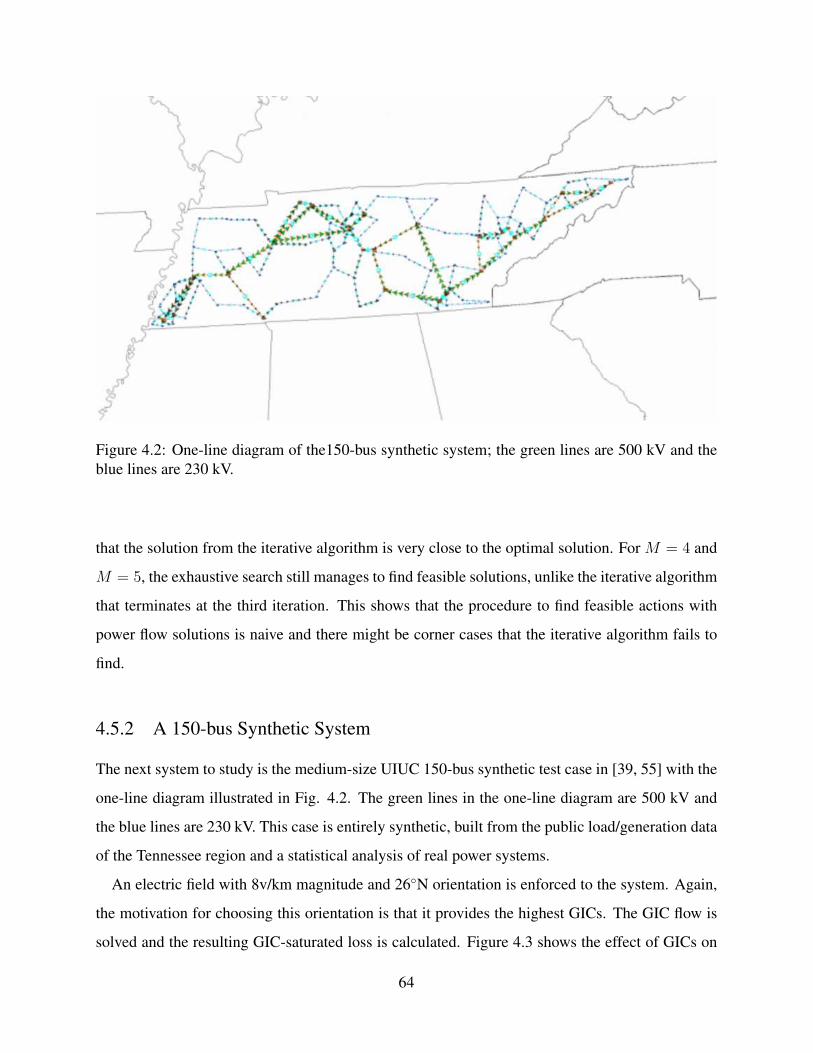
Figure 4.2: One-line diagram of the150-bus synthetic system; the green lines are 500 kV and theblue lines are 230 kV.
that the solution from the iterative algorithm is very close to the optimal solution. For M = 4 and
M = 5, the exhaustive search still manages to find feasible solutions, unlike the iterative algorithm
that terminates at the third iteration. This shows that the procedure to find feasible actions with
power flow solutions is naive and there might be corner cases that the iterative algorithm fails to
find.
4.5.2 A 150-bus Synthetic System
The next system to study is the medium-size UIUC 150-bus synthetic test case in [39, 55] with the
one-line diagram illustrated in Fig. 4.2. The green lines in the one-line diagram are 500 kV and
the blue lines are 230 kV. This case is entirely synthetic, built from the public load/generation data
of the Tennessee region and a statistical analysis of real power systems.
An electric field with 8v/km magnitude and 26N orientation is enforced to the system. Again,
the motivation for choosing this orientation is that it provides the highest GICs. The GIC flow is
solved and the resulting GIC-saturated loss is calculated. Figure 4.3 shows the effect of GICs on
64
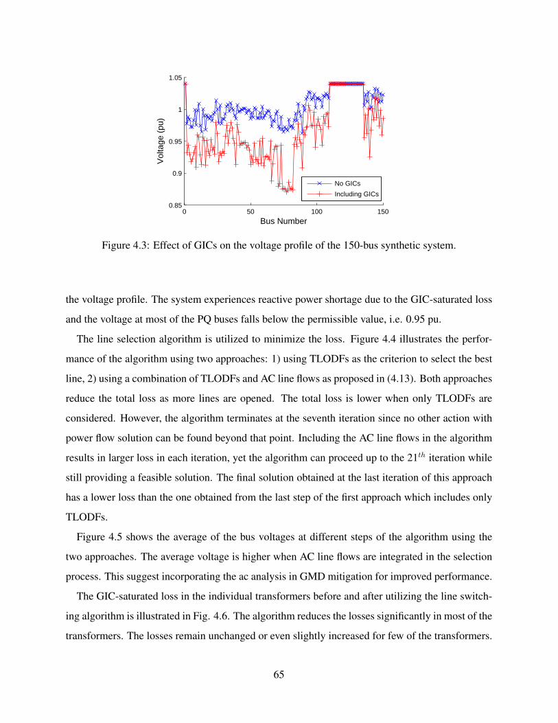
0 50 100 1500.85
0.9
0.95
1
1.05
Bus Number
Vol
tage
(pu
)
No GICs
Including GICs
Figure 4.3: Effect of GICs on the voltage profile of the 150-bus synthetic system.
the voltage profile. The system experiences reactive power shortage due to the GIC-saturated loss
and the voltage at most of the PQ buses falls below the permissible value, i.e. 0.95 pu.
The line selection algorithm is utilized to minimize the loss. Figure 4.4 illustrates the perfor-
mance of the algorithm using two approaches: 1) using TLODFs as the criterion to select the best
line, 2) using a combination of TLODFs and AC line flows as proposed in (4.13). Both approaches
reduce the total loss as more lines are opened. The total loss is lower when only TLODFs are
considered. However, the algorithm terminates at the seventh iteration since no other action with
power flow solution can be found beyond that point. Including the AC line flows in the algorithm
results in larger loss in each iteration, yet the algorithm can proceed up to the 21th iteration while
still providing a feasible solution. The final solution obtained at the last iteration of this approach
has a lower loss than the one obtained from the last step of the first approach which includes only
TLODFs.
Figure 4.5 shows the average of the bus voltages at different steps of the algorithm using the
two approaches. The average voltage is higher when AC line flows are integrated in the selection
process. This suggest incorporating the ac analysis in GMD mitigation for improved performance.
The GIC-saturated loss in the individual transformers before and after utilizing the line switch-
ing algorithm is illustrated in Fig. 4.6. The algorithm reduces the losses significantly in most of the
transformers. The losses remain unchanged or even slightly increased for few of the transformers.
65

0 5 10 15 2020
25
30
35
40
45
50
Number of Opened Lines
Rea
ctiv
e P
ower
Los
s (p
u)
TLODFTLODFs and Line Flows
Figure 4.4: Total GIC-saturated reactive power loss in terms of the number of opened lines usingthe proposed line switching algorithm.
Developing techniques to restrict the losses in each transformer as opposed to the minimizing the
overall loss will be an interesting future study.
4.5.3 2000-bus Synthetic System
The last system to study is the 2000-bus synthetic system [55, 79]. Similar to the 150-bus synthetic
system, this case is entirely synthetic and built from the public load/generation data of the region
using real power systems statistical analysis.
An electric field with 8v/km magnitude and 91N orientation (the direction with highest GICs)
is enforced to the system. The GIC-saturated loss is calculated and the line selection algorithm is
applied to find the best switching strategy. The system is large and the running time is significant,
i.e. 3047.7 seconds when the number of opened lines is 120. The computations are performed on
a Dell XPS 700 system with Intel core i7. The running time may be reduced through the fast line
selection algorithm. Figure 4.7 illustrates the total loss in terms of the number of opened lines for
two scenarios:
(A) All the lines are considered and the full TLODF matrix is updated in each iteration.
(B) 200 critical lines are selected and the full TLODF matrix is not updated (C = 200, U is not
66

0 5 10 15 200.935
0.94
0.945
0.95
0.955
0.96
0.965
Number of Opened Lines
Ave
rage
Bus
Vol
tage
(pu
)
TLODF
TLODFs and Line Flows
Figure 4.5: Average bus voltage in terms of the number of opened lines using the proposed lineswitching algorithm.
Table 4.3: Analyzing the Computational Complexity of the Iterative Line Switching Algorithmunder Different Scenarios
TLODF UpdateFrequency
Number ofCritical Lines
RunningTime (s)
Total Loss(pu)
Error(%)
Time Ratio(%)
A 1 3024 3047.7 3.62 0 100B - 200 124.4 4.18 15.61 4.08C 10 200 320 3.72 2.47 10.49D 40 200 181 3.71 2.72 5.93E 40 100 105.2 3.72 2.72 3.45
defined).
It is observed that the fast scenario (Scenario B) provides the same loss as the full calculation
(Scenario A) when the number of opened lines is smaller than 40 and start to diverge afterwards.
Hence, it is reasonable to recalculate the TLODFs and update the list of critical lines after each 40
iterations, i.e. U = 40.
Table 4.3 presents the running time and accuracy of the algorithm for different values of U (the
TLODF update frequency) and C (and the number of critical lines). The first two scenarios in the
table are the same scenarios presented earlier. The accuracy of each scenario is presented in terms
of the percentage error between its resulting loss and the one from the full search (Scenario A).
67

0 10 20 30 40 50 600
0.5
1
1.5
2
2.5
3
3.5
4
Transformer ID
Rea
ctiv
e P
ower
Los
s (p
u)
No Action
Topology Control
Figure 4.6: GIC-saturated loss in the individual transformers before and after utilizing the topologycontrol.
The presented time ratio denotes the ratio of the running time of each scenario to the full search.
Using the fast search with 100 critical lines and the TLODF update frequency of 40 (Scenario E)
can provide the same performance as the full search with 2.72% error at only 3.45% of its running
time.
4.6 Conclusions
In this chapter, a line switching algorithm is developed to mitigate the negative impacts of GMDs.
The algorithm minimizes the GIC-saturated reactive power loss based on TLODFs (counterparts
of LODFs in GIC analysis). Some aspects of the ac analysis are considered to provide sufficient
ac-related security measures. The computational complexity of the algorithm is analyzed and
heuristics are utilized to reduce its running time for large-system applications. The algorithm
performance is evaluated through numerical results using the small 20-bus system, the medium-
size 150-bus synthetic system and the large 2000-bus synthetic case. The main observations are as
follows:
• Considering the AC line flows as an additional criterion for selecting the best lines improves
68

0 20 40 60 80 100 12070
80
90
100
110
120
130
Number of Opened Lines
Rea
ctiv
e P
ower
Los
s (p
u)
A) Updated TLODFsB) Constant TLODFs, 200 Critical Lines
Figure 4.7: Effect of the TLODF update frequency on the performance of the algorithm for the2000-bus synthetic system.
the overall performance in terms of AC and DC power flow solutions.
• The optimality of the proposed strategy was evaluated by comparing it with the exhaustive
search. The numerical results indicate that while the algorithm does not find the optimal
solution, it gets very close to it (finds the second best solution).
• The heuristics used for fast computation are evaluated through case studies on the 2000-bus
synthetic system. It was observed that that the running time can be reduced by up to 97%
while the loss reduction is compromised by only 2%.
The chapter suggests several directions for future research. First, the proposed algorithm min-
imizes the total loss in the system, but does not impose any limit on the loss of individual trans-
formers. The algorithm can be further refined to restrict the losses in each transformer while mini-
mizing the total loss. Second, this chapter focuses on line switching as the remedial action. Future
research can extend this framework to other types of actions such as shunt capacitor switching and
neutral blocking devices.
69

CHAPTER 5
GMD MODEL VALIDATION BASED ONSINGULAR VALUE DECOMPOSITION
5.1 Introduction
This chapter proposes singular value decomposition (SVD) to validate the GIC model solely
through the measurements and independent of the network information. Under the uniform E-
field, there exists a linear relation between the GICs and the E-field. This enables development of
an SVD-based technique to estimate the E-field and eventually validate the model. This framework
is later extended to include more realistic non-uniform E-fields and its effectiveness is verified us-
ing a practical 20-bus test case. GMD modeling is a fundamental part of the GMD mitigation and
the model validation tool presented in this chapter can contribute to the resiliency against GMDs
by improving the associated models.
The chapter is organized as follows: SVD-based analysis is presented in Section 5.2, which
introduces the singular vectors for estimating the E-field. Section 5.3 presents the proposed vali-
dation framework using a 20-bus test case. In Section 5.4, the GIC model is modified to account
for non-uniform E-field and its validity is examined using SVD and through simulation. Section
5.5 presents a conclusion and directions for future work.
5.2 Singular Value Decomposition
The GIC model is defined in (3.14) and reproduced below:
Z = HX + V
70
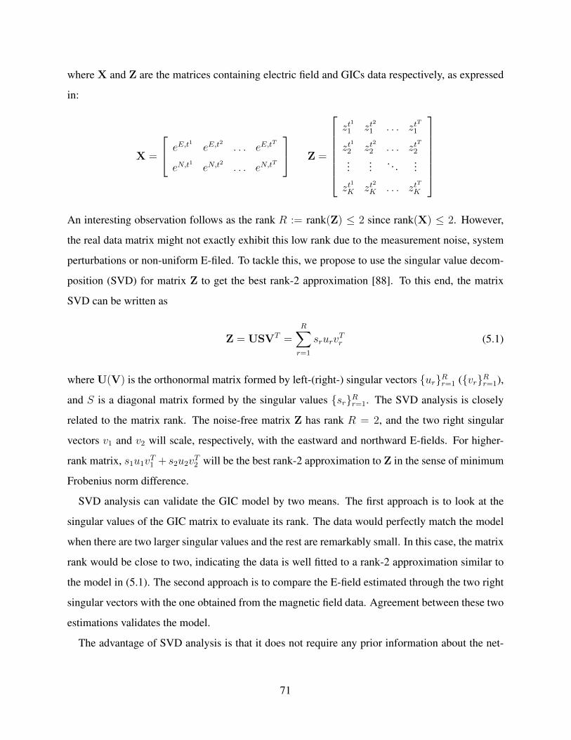
where X and Z are the matrices containing electric field and GICs data respectively, as expressed
in:
X =
eE,t1eE,t
2. . . eE,t
T
eN,t1eN,t
2. . . eN,t
T
Z =
zt
1
1 zt2
1 . . . ztT
1
zt1
2 zt2
2 . . . ztT
2
...... . . . ...
zt1
K zt2
K . . . ztT
K
An interesting observation follows as the rank R := rank(Z) ≤ 2 since rank(X) ≤ 2. However,
the real data matrix might not exactly exhibit this low rank due to the measurement noise, system
perturbations or non-uniform E-filed. To tackle this, we propose to use the singular value decom-
position (SVD) for matrix Z to get the best rank-2 approximation [88]. To this end, the matrix
SVD can be written as
Z = USVT =R∑r=1
srurvTr (5.1)
where U(V) is the orthonormal matrix formed by left-(right-) singular vectors urRr=1 (vrRr=1),
and S is a diagonal matrix formed by the singular values srRr=1. The SVD analysis is closely
related to the matrix rank. The noise-free matrix Z has rank R = 2, and the two right singular
vectors v1 and v2 will scale, respectively, with the eastward and northward E-fields. For higher-
rank matrix, s1u1vT1 + s2u2vT2 will be the best rank-2 approximation to Z in the sense of minimum
Frobenius norm difference.
SVD analysis can validate the GIC model by two means. The first approach is to look at the
singular values of the GIC matrix to evaluate its rank. The data would perfectly match the model
when there are two larger singular values and the rest are remarkably small. In this case, the matrix
rank would be close to two, indicating the data is well fitted to a rank-2 approximation similar to
the model in (5.1). The second approach is to compare the E-field estimated through the two right
singular vectors with the one obtained from the magnetic field data. Agreement between these two
estimations validates the model.
The advantage of SVD analysis is that it does not require any prior information about the net-
71
work. This method estimates the E-field through the GIC measurements without using any ad-
ditional network information. SVD analysis also benefits from robustness to different types of
uncertainties in the system. The three common sources of error with significant impact on the GIC
model are recognized as follows:
1. White Gaussian noise: The noise generated by many natural sources appears in the form
of white Gaussian noise. GIC measurements are often perturbed by this type of noise.
2. Incorrect meter scaling: It is possible that the GICs obtained from measuring devices
differ from the actual GICs by some constants. This type of error is caused by the incorrect
meter scaling.
3. Outliers: The linear GIC model assumes uniform E-field over all measurements. Natural
factors such as geographic distant, regional ground structure or neighboring water bodies
could result in a different E-field for a transformer. The GIC measured at such a transformer
does not agree with the model and is considered as outlier.
The robustness of the SVD-based method to these three types of uncertainties is evaluated later
through simulation.
5.3 Numerical Results Using a Test Case
In this section, the effectiveness of the proposed model validation techniques is evaluated through
simulation. For this study, the 20-bus system in [38] is investigated with the one-line diagram
illustrated in Fig. 4.1. For this testing we will superimpose actual GMD data from March 9,
2012, on this fictitious test system. On March 9, the geomagnetic storm began at 2:00 UTC and
reached a very high level in the following hours. The magnetic field data used here are from values
measured at the Fredericksburg observatory, located in the US at a latitude/longitude of 38.205N ,
77.373W . The E-field obtained from this magnetic field is enforced on the system and the induced
GICs are determined by solving the GIC flows using PowerWorld Simulator with the GIC add-on.
To simulate the system perturbations and measurement noise, white Gaussian random noise with
72
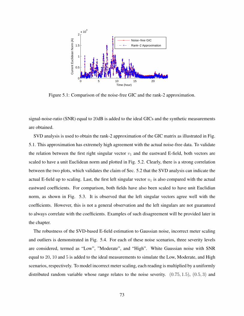
0 5 10 15 200
0.5
1
1.5
2x 10
4
Time (hour)
Cur
rent
Euc
lidea
n N
orm
(A
)
Noise−free GIC
Rank−2 Approximation
Figure 5.1: Comparison of the noise-free GIC and the rank-2 approximation.
signal-noise-ratio (SNR) equal to 20dB is added to the ideal GICs and the synthetic measurements
are obtained.
SVD analysis is used to obtain the rank-2 approximation of the GIC matrix as illustrated in Fig.
5.1. This approximation has extremely high agreement with the actual noise-free data. To validate
the relation between the first right singular vector v1 and the eastward E-field, both vectors are
scaled to have a unit Euclidean norm and plotted in Fig. 5.2. Clearly, there is a strong correlation
between the two plots, which validates the claim of Sec. 5.2 that the SVD analysis can indicate the
actual E-field up to scaling. Last, the first left singular vector u1 is also compared with the actual
eastward coefficients. For comparison, both fields have also been scaled to have unit Euclidian
norm, as shown in Fig. 5.3. It is observed that the left singular vectors agree well with the
coefficients. However, this is not a general observation and the left singulars are not guaranteed
to always correlate with the coefficients. Examples of such disagreement will be provided later in
the chapter.
The robustness of the SVD-based E-field estimation to Gaussian noise, incorrect meter scaling
and outliers is demonstrated in Fig. 5.4. For each of these noise scenarios, three severity levels
are considered, termed as “Low”, ”Moderate”, and “High”. White Gaussian noise with SNR
equal to 20, 10 and 5 is added to the ideal measurements to simulate the Low, Moderate, and High
scenarios, respectively. To model incorrect meter scaling, each reading is multiplied by a uniformly
distributed random variable whose range relates to the noise severity. (0.75, 1.5), (0.5, 3) and
73

0 5 10 15 20−0.015
−0.01
−0.005
0
0.005
0.01
0.015
Time (hour)
Nor
mal
ized
E−
field
Actual Field
Singular Vector V1
Figure 5.2: Comparison of the actual northward E-field and the estimate using v1.
(0.25, 6) are the three ranges used to model the severity levels with the wider range corresponding
to more severe scenario. Finally, the outliers are modeled by using a different E-field to generate
them. The E-field is based on actual data for the same time period from the Ottawa observatory,
located in Canada at a latitude/longitude of 45.403N , 75.552W . The Ottawa data is used to
simulate the outliers whereas the normal measurements are generated by the Fredericksburg data.
The severity level is increased from Low to High by increasing the number of outliers from 1
to 3. Monte Carlo simulation with 100 realizations is investigated to perfectly simulate all types
of uncertainties. It is observed that the E-field estimation is very robust to Gaussian noise and
incorrect scaling. Although the robustness of the estimator to outliers is relatively low, it still
provides sufficient accuracy and the error stays below 3.5%.
The first left singular vector is compared with the eastward coefficients under different scenarios
and its normalized error is plotted in Fig. 5.5. The interesting observation is that the coefficient
estimation is very robust to Gaussian noise, yet is very sensitive to incorrect scaling and outliers.
The sensitivity to outliers is especially very high and the error goes as high as 100%. This suggests
that the SVD-based coefficient estimation is not valid in the presence of these types of noise.
74

0 5 10 15−0.25
−0.2
−0.15
−0.1
−0.05
0
0.05
0.1
0.15
Transformer Number
Eas
twar
d C
oeffi
cien
t
Actual Field
Singular vector U1
Figure 5.3: Comparison of the actual northward coefficients with the estimate using the rightsingular vector u1.
5.4 Non-uniform Electric Field
The E-field varies with the magnetic field and the surface impedance as given in (3.9) and repro-
duced here:
E(ω) =1
µ0
Z(ω)B(ω)
where Z is the Earth surface impedance, B is the magnetic flux density, ω is the frequency and
µ0 is the permeability of free space. The surface impedance depends on the regional tectonic
structure and is calculated through the local conductivity model [89]. The magnetic field varies
with the geomagnetic latitude. Preliminary studies consider the effect of both latitude and local
conductivity on the E-field to be linear and model it through scaling factor as given by [90]:
E = αβ Eref (5.2)
where α and β are the scaling factors to account for the local earth conductivity structure and the
geomagnetic latitude respectively, andEref is the reference E-field. The GIC of the kth transformer
75

Gaussian Noise Incorrect Scaling Outliers0
1
2
3
4
5
6
Nor
mal
ize
Err
or (
%)
Low
Moderate
High
Figure 5.4: Robustness of the SVD-based E-field estimation to different system uncertainties.
Gaussian Noise Incorrect Scaling Outliers0
20
40
60
80
100
Nor
mal
ize
Err
or (
%)
Low
Moderate
High
Figure 5.5: Accuracy of the SVD-based coefficient estimation under different system uncertainties.
at the nth time instant is given by:
ztn
k = HkEtn
k = HkλkEtn
ref (5.3)
where λk := αkβk is the scaling factor for the kth transformer. Writing this for all the measure-
ments at all the time instances gives rise to:
Y = [λ1H1|λ2H2| · · · |λKHK ]TX = HCX (5.4)
76

2 3 4 5 6 7 8 9 10 11
−0.02
−0.01
0
0.01
0.02
Time (hour)
Nor
mal
ized
E−
Fie
ld
IP−3 Field
PT−1 Field
Estimate
Figure 5.6: Non-uniform E-field scenario with different conductivity: estimated and actual E-fieldsin north direction.
where HC is the modified coefficient matrix to account for the non-uniform E-field. Note that the
rank of the GIC matrix is still two since rank(X) ≤ 2.
Next, the impacts of these scaling factors are considered through simulation using the 20-bus
test case. Two non-uniform E-field scenarios are considered and SVD is used to validate the
model under these scenarios. The first scenario considers two E-fields both generated by the same
magnetic field (Fredericksburg), but two different conductivity models. These models relate to
the Piedmont (PT-1) and the lower Michigan Interior Plains (IP-3). The E-field generated by the
PT-1 model is enforced to the substations 1, 2 and 3 whereas the rest of the network is subject to
the IP-3 E-field. The induced GICs are determined by solving the GIC flow program and SVD is
used to estimate the electric field. The estimated E-field, the IP-3 E-field enforced to the first three
substations and the PT-1 field enforced to the rest of the network are normalized and plotted in
Fig. 5.6. It is observed that the IP-3 and PT-1 E-fields are highly correlated with 0.97 correlation
coefficient. This indicates that the effect of the local conductivity on the E-field is closely linear
and modeling it through the scaling factor λ is valid and accurate. This is further verified by
observing the agreement between the estimated E-field with the two E-fields in the network.
The second scenario studies the effect of the geomagnetic latitude on the E-field. In this sce-
nario, the two E-fields are generated by two different magnetic data (Fredericksburg and Ottawa),
but the same conductivity model (IP-3). The Ottawa E-field is enforced to the first three substa-
77
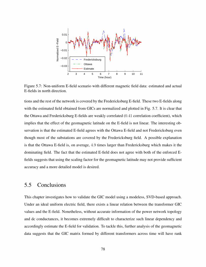
2 3 4 5 6 7 8 9 10 11
−0.03
−0.02
−0.01
0
0.01
Time (hour)
Nor
mal
ized
E−
Fie
ld
Fredericksburg
Ottawa
Estimate
Figure 5.7: Non-uniform E-field scenario with different magnetic field data: estimated and actualE-fields in north direction.
tions and the rest of the network is covered by the Fredericksburg E-field. These two E-fields along
with the estimated field obtained from GICs are normalized and plotted in Fig. 5.7. It is clear that
the Ottawa and Fredericksburg E-fields are weakly correlated (0.41 correlation coefficient), which
implies that the effect of the geomagnetic latitude on the E-field is not linear. The interesting ob-
servation is that the estimated E-field agrees with the Ottawa E-field and not Fredericksburg even
though most of the substations are covered by the Fredericksburg field. A possible explanation
is that the Ottawa E-field is, on average, 4.9 times larger than Fredericksburg which makes it the
dominating field. The fact that the estimated E-field does not agree with both of the enforced E-
fields suggests that using the scaling factor for the geomagnetic latitude may not provide sufficient
accuracy and a more detailed model is desired.
5.5 Conclusions
This chapter investigates how to validate the GIC model using a modeless, SVD-based approach.
Under an ideal uniform electric field, there exists a linear relation between the transformer GIC
values and the E-field. Nonetheless, without accurate information of the power network topology
and dc conductances, it becomes extremely difficult to characterize such linear dependency and
accordingly estimate the E-field for validation. To tackle this, further analysis of the geomagnetic
data suggests that the GIC matrix formed by different transformers across time will have rank
78

2 and the right singular vectors can be used to infer the E-field. This SVD-based approach has
validated the linear relation using a realistic test case. The validation framework is also extended
to account for non-uniform E-field and is successfully demonstrated through simulation.
79
CHAPTER 6
PARAMETER-BASED GMD MODEL VALIDATION
6.1 Introduction
Providing resiliency to GMDs is very challenging and it is desired to utilize all the available in-
formation on the network to achieve this goal. This chapter proposes a validation technique which
improves over the SVD-based one in Chapter 5 by utilizing the available parameters. In this tech-
nique, first, the conventional GIC model is modified to account for the system uncertainties. Then,
a validation framework is built upon this modified model. This framework is successfully demon-
strated using a PowerWorld case study and its performances is evaluated. The effectiveness of
the proposed technique in handling real system uncertainties is validated through actual GIC data
provided by the American Transmission Company (ATC).
The chapter is organized as follows: Model validation under system uncertainties is presented
in Section 6.3. Section 6.4 demonstrates the proposed technique using the 20-bus PowerWorld test
case, while the more interesting real data validation is given in Section 6.5 with transformer neutral
current measurements from ATC. Section 6.6 presents a conclusion and directions for future work.
6.2 Determination of the Transformers Coefficients
There are two coefficients associated with each transformer and the GIC model in (3.8) can be
rewritten as:
I = [HE | HN ]×
EE
EN
(6.1)
80

where HE and HN are the eastward and northward coefficients. An interesting observation is that
the GICs are equal to the eastward coefficients when EE is one and EN is zero. Similarly, the
GICs are equal to the northward coefficients when EE is zero and EN is one. This will be a basis
for finding the coefficients as described in the following algorithm.
Step 1: An eastward E-field with unity magnitude is enforced to the system and the resulting
GICs are calculated. According to (6.1), the eastward coefficients are equal to the GICs under
this condition.
Step 2: A northward E-field with unity magnitude is enforced to the system and the northward
coefficients are calculated similar to Step 1.
This algorithm requires calculation of the GICs induced by an enforced E-field. This can be
done through basic circuit laws e.g. KVL, KCL and Ohm’s law. Alternatively, a commercial
power system software like PowerWorld Simulator may be used to conduct such calculations.
6.3 Model Validation Under Actual Measurements
In practice, the GIC model in (3.14) fails to represent the actual measurements as they are subjected
to different types of noise and system uncertainties. To account for such uncertainties, the GIC
model is modified by introducing a scale for each measurement as given by:
Y = S H X + N (6.2)
where S is a diagonal matrix with the scales on its diagonal. If properly defined, the scales can
capture the system uncertainties. The GIC real data may be used to find such scales as described
in Algorithm 6. In the algorithm, Diag() of a vector is a diagonal matrix with the vector’s entries
on its diagonal, ~1 is an all-one vector, Sum() of a matrix returns the sum of all its entries and K is
the number of measurements.
The coefficient matrix depends on the network topology and resistances and its accuracy de-
pends on the available network information. Most of the network parameters required for con-
structing the coefficient matrix are part of the standard power flow models and are accurately
81

Algorithm 6 Scales Calculation1: procedure SCALES CALCULATION(Y, H)2: Initialize all the priori scales to one: S = Diag(~1).3: Initialize the posteriori scales to zero: S+ = Diag(~0).4: Define the convergence tolerance, ε.5: while | S+ − S |> ε do6: Update the priori scales by S = S+
7: Estimate the E-field using:X = (HTSTSH)−1HTSTY.
8: Calculate the posteriori scales by:S+ = Diag(Y)Diag−1(HX).
9: Normalize the scales by S+ = KS+
Sum(S+).
10: end while11: return S12: end procedure
available. The only piece of information which may not be available, but has high impacts is the
substation grounding resistance, which is the effective grounding resistance of the substation and
includes the ground grid and the emanating ground paths due to shield wire grounding. Techniques
are available in the literature to measure this parameter [46], yet many factors can compromise the
measurement and consequently introduce error to the GIC model validation. First, external objects
such as water pipeline and adjacent railroad tracks distort the earth potential contours. Second,
sources of dc current such as dc railroad tracks, pipelines cathodic protection systems and dc
transmission lines produce stray currents which interfere with the grounding resistance measure-
ments. Third, the resistance of the electrodes used for the measurements can introduce error if
the substation being tested has low resistivity. Last, the grounding resistance mostly depends on
the humidity, salt level or temperature and therefore is time-variant. Accurate measurement of the
grounding resistance is very challenging and the available data (if any) is often inaccurate. Assign-
ing the proper scales to the substation accounts for the inaccuracy of its grounding resistance.
The scales can be used to evaluate how well the GICs at a particular transformer agree with the
model. In practice, not all the measurements conform to the model and some of the readings may
exhibit different behavior. A possible reason for such divergent behaviors is non-uniform E-field.
The linear GIC model is valid only when the E-field is uniform over the investigated area. When
the geographic location of a transformer is too far from the others, its E-field may differ and its
82
GIC will not agree with the model. The proposed scale estimation technique detects the outlier
measurements by assigning them zero scale and eventually excludes them from the dataset. An
example of using the scales to detect outliers will be provided later.
Compared to the SVD-based analysis presented in [59], the proposed framework has several
advantages owing to the additional network parameters. First, the proposed framework can validate
the measurements independently and identify those that do not conform to the model, whereas
the SVD analysis determines the validity of the measurements all together without providing any
insight on the individual measurements. Second, the proposed method provides additional tools
for validating the parameter accuracy. The method utilizes the network parameters to estimate
the E-field. Hence, the agreement between this estimation and the one from the magnetic field
data validates the accuracy of the assumed parameters. Last, the proposed model provides more
accurate E-field estimation than the SVD-based one, which makes the validation framework built
upon it more effective. Numerical results indicate that the first left singular of the SVD analysis
perfectly captures the eastward E-field, yet the second left singular fails to estimate the northward
E-field accurately. The comparison between the two methods will be provided later through case
studies as well as real data analysis, and the advantages of the proposed technique discussed here
will be demonstrated.
6.4 Numerical Results Using a Test Case
In this section and the next, the effectiveness of the proposed validation technique is evaluated.
This section uses the fictitious 20-bus system from [38], whereas in Section 6.5 the technique is
evaluated using actual data GIC neutral currents for five transformers located in the ATC footprint
for a GMD that occurred on March 9, 2012. For consistency, the same March 9, 2012, data will be
used with the 20-bus case.
On March 9 the geomagnetic storm began at 2:00 UTC and reached a very high level in the
following hours. The magnetic field data used here are from values measured at the US Geological
Survey (USGS) Fredericksburg Geomagnetic Observatory, located in the US at a latitude/longi-
tude of 38.205N , 77.373W . The reason for choosing this observatory is, again, to maintain
83

consistency with the results in Section 6.5. The transformers used in Section 6.5 are located in the
ATC footprint and Fredericksburg is the closest observatory to these transformers.
The E-field obtained from the Fredericksburg magnetic field is enforced on the system and the
induced GICs are determined by solving the GIC flows using PowerWorld Simulator with the GIC
add-on. White Gaussian random noise with signal-noise-ratio (SNR) equal to 20dB is added to the
ideal GICs to simulate the system noise, and the synthetic measurements are obtained.
To evaluate the performance of the model validation framework under different uncertainties,
three scenarios are considered, each focusing on one type of uncertainty:
1. Inaccurate Coefficients Scenario: In this scenario, the available coefficients at the eighth
and ninth transformers are two times larger than the actual ones (100% error). This could be
caused by the inaccurate substation grounding resistances. In practice, the coefficients may have
much lower error and this study considers the worst case scenarios.
2. Outliers Scenario: In this scenario, the measurements at the eighth and ninth transformers
are enforced to be outliers. Outliers are considered to be measurements which are generated by a
different E-field. The E-field data at The Natural Resources Canada (NRCan) Ottawa Geomagnetic
Observatory is used to simulate the outliers whereas the normal measurements are generated by the
Fredericksburg data. Ottawa observatory is located in Canada at a latitude/longitude of 45.403N ,
75.552W .
3. Low Uncertainty Scenario: This scenario considers the ideal case when the substation
grounding resistances are accurate and no outlier exists in the measurements.
The transformer scales can account for the inaccurate coefficients. Figure 6.1 illustrates the
scales under the first scenario where the assumed coefficients at the eighth and ninth transformers
are double the actual ones. According to the figure, the scales for these transformers take the value
of 0.5 to compensate for this inaccuracy. A correct estimate of the coefficients can be obtained
through multiplying the assumed coefficients by their corresponding scales as shown in Fig. 6.2.
The transformer scales can be used to detect the measurement outliers as illustrated in Fig.
6.3. The readings from the eighth and ninth transformers are enforced to be outliers and the scale
estimation technique successfully detects them and eliminates them from the model by assigning
them zero scales.
The 20-bus system has two shunt capacitors at bus 4 and 16. Numerical results indicate that
84

0 5 10 150.4
0.6
0.8
1
1.2
1.4
Transformer Number
Sca
le
Figure 6.1: Transformer scales under the inaccurate coefficients scenario.
disconnecting these capacitors does not affect the proposed framework. This is because the GIC
calculation is based on steady state dc analysis in which the capacitors act as open circuit. Hence,
disconnecting them does not change the GIC model. The effect becomes significant when AC
analysis is performed as opposed to dc. Power flow is solved including GICs and it is observed that
connecting the shunt capacitors provides reactive power support and improves the voltage profile.
The framework is robust to power filters and static synchronous compensator (STATCOM) devices
as well since they only affect the AC analysis and not the dc.
Next, the performance of the proposed model is compared with the SVD-based technique pre-
sented in [59]. Table 6.1 presents the accuracy of the two methods in estimating the E-field. For
reference, the results for the conventional model in (3.14) are also included. Pearson correlation
coefficient is used to measure the correlation between the estimated and the actual E-field with the
following definition:
ρX,Y =cov(X, Y )
σXσY(6.3)
where ρX,Y and cov(X, Y ) are the Pearson correlation and covariance between signals X and Y ,
respectively, and σ is the standard deviation. The comparison is performed for the three uncer-
tainty scenarios described earlier, which are Inaccurate Coefficients, Outliers, and Low Uncer-
tainty. These scenarios are denoted by “Scen1”, “Scen2” and “Scen3” in the table, respectively. In
85
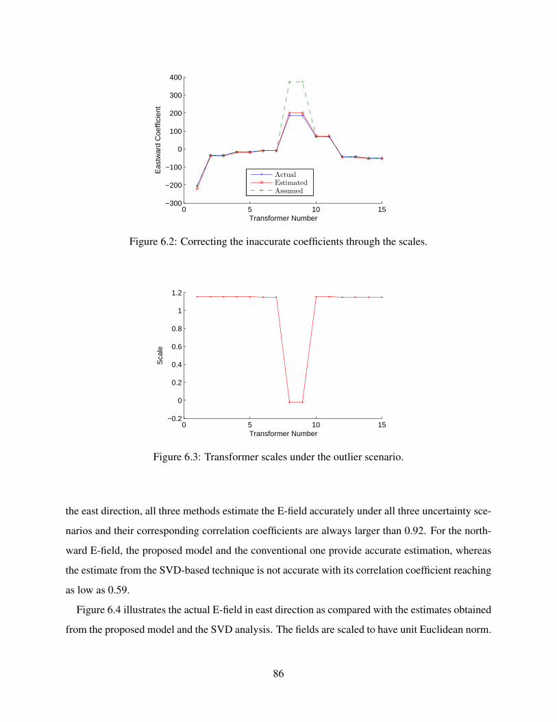
0 5 10 15−300
−200
−100
0
100
200
300
400
Transformer Number
Eas
twar
d C
oeffi
cien
t
Actual
Estimated
Assumed
Figure 6.2: Correcting the inaccurate coefficients through the scales.
0 5 10 15−0.2
0
0.2
0.4
0.6
0.8
1
1.2
Transformer Number
Sca
le
Figure 6.3: Transformer scales under the outlier scenario.
the east direction, all three methods estimate the E-field accurately under all three uncertainty sce-
narios and their corresponding correlation coefficients are always larger than 0.92. For the north-
ward E-field, the proposed model and the conventional one provide accurate estimation, whereas
the estimate from the SVD-based technique is not accurate with its correlation coefficient reaching
as low as 0.59.
Figure 6.4 illustrates the actual E-field in east direction as compared with the estimates obtained
from the proposed model and the SVD analysis. The fields are scaled to have unit Euclidean norm.
86

Table 6.1: Accuracy Comparison of the E-field Estimation Techniques for the Test Case
EstimationTechnique
Eastward E-Field Northward E-FieldScen1 Scen2 Scen3 Scen1 Scen2 Scen3
Proposed 1.000 1.000 1.000 1.000 1.000 1.000Conventional 0.997 0.992 1.000 0.999 0.998 1.000SVD 0.974 0.927 0.974 0.710 0.591 0.710
2 3 4 5 6 7 8 9 10 11
−0.2
−0.15
−0.1
−0.05
0
0.05
0.1
0.15
0.2
Time (hour)
Nor
mal
ized
E−
Fie
ld
Actual FieldProposed ModelSVD
Figure 6.4: Comparison of the eastward E-field estimation using different methods for the testcase.
The agreement between the estimated and actual fields verifies the accuracy for both methods.
Figure 6.5 demonstrates similar comparison for E-field in north direction. In this direction, the
estimate from the proposed model has extremely high agreement with the actual field whereas the
SVD analysis fails to provide good accuracy. The estimate from the conventional model is not
included in Fig. 6.4 and Fig. 6.5 for better clarity, as it is perfectly aligned with the estimate from
the proposed model. The E-field estimated by the conventional model differs from that estimated
by the proposed model only by a scaling factor, and hence the normalized fields in the figures are
aligned.
The last validation test is to study the accuracy of different techniques in estimating the individ-
ual GIC measurements. The E-fields estimated by the conventional and proposed model are used in
their corresponding GIC flow equations, which are (3.14) for the conventional model and (6.2) for
87

2 3 4 5 6 7 8 9 10 11
−0.15
−0.1
−0.05
0
0.05
0.1
0.15
0.2
0.25
Time (hour)
Nor
mal
ized
E−
Fie
ld
Actual FieldProposed ModelSVD
Figure 6.5: Comparison of the northward E-field estimation using different methods for the testcase.
Table 6.2: Percentage Error Norm in Estimating GICs Based on Different Techniques
Estimation Technique Scen1 Scen2 Scen3Proposed 4.91% 5.22% 5.01%Conventional 48.29% 66.45% 5.01%SVD 4.91% 5.21 % 5.00%
the proposed one, and the estimated GICs are obtained. This estimation is then compared with the
actual GICs which was initially used to estimate the E-field. The SVD-based technique estimates
GICs through rank-2 approximation. Table 6.2 presents the estimation error for the investigated
techniques with error defined as
Error =‖Y −Y‖F‖Y‖F
(6.4)
where Y is the matrix of estimated GICs and ‖ · ‖F is the Frobenius norm. It is observed that the
SVD analysis and the proposed model estimate the GICs accurately for all uncertainty scenarios.
The conventional model estimates the GICs accurately under the ideal scenario, but its estimation
error increases up to 66% in the presence of grounding resistance uncertainty or outliers.
88

Figure 6.6: Geographic location of the investigated ATC transformers.
6.5 Numerical Results for Real Data
In this section, the GIC model is validated using real data measurements provided by ATC. This
study focuses on the neutral current measurements of five transformers near the Wisconsin/Michi-
gan area with the locations illustrated in Fig. 6.6. The geographical proximity of the Fredericks-
burg magnetometer to the ATC footprint makes using its data relevant to this study.
The GIC data for the March 9, 2012, storm is chosen primarily for the analysis, as plotted in Fig.
6.7. The transformers are indexed from 1 to 5. The highest GIC observed at these transformers is
27 A. Records of previous storms indicate that GICs can reach up to 330 A for more vulnerable
locations and more severe storms [10]. Such observations indicate that the existing infrastructure
including the shielding techniques does not protect the substations from GMDs. The GICs are
derived from the E-field induced over long transmission lines and are sunk into the ground through
the substation grounding. The shielding techniques may protect a small range, but fail to block
the GICs coming from long transmission lines. It is observed that at the transformers TR4, and
TR5, the absolute value of the current is measured and the direction is missing. An effective data
preprocessing technique is used to retrieve the direction as presented in the following.
89
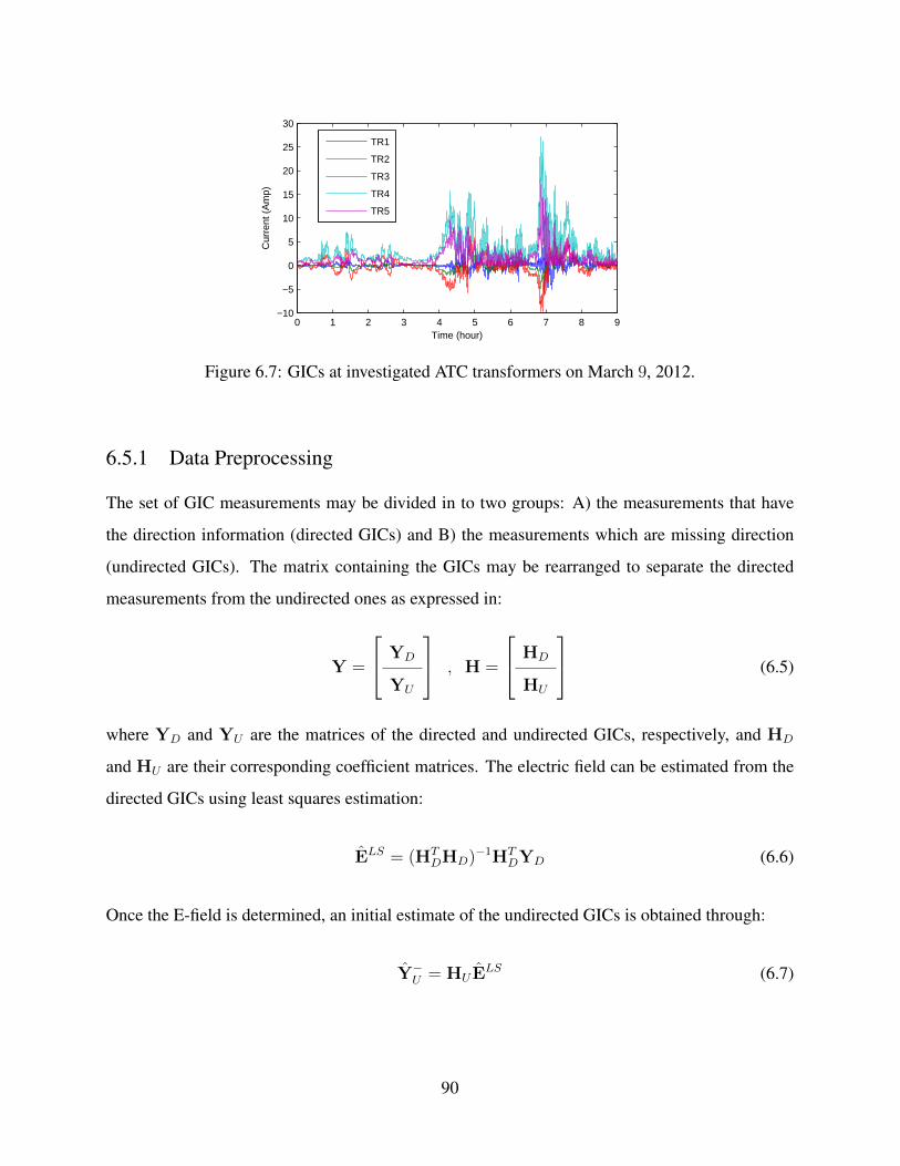
0 1 2 3 4 5 6 7 8 9−10
−5
0
5
10
15
20
25
30
Time (hour)
Cur
rent
(A
mp)
TR1
TR2
TR3
TR4
TR5
Figure 6.7: GICs at investigated ATC transformers on March 9, 2012.
6.5.1 Data Preprocessing
The set of GIC measurements may be divided in to two groups: A) the measurements that have
the direction information (directed GICs) and B) the measurements which are missing direction
(undirected GICs). The matrix containing the GICs may be rearranged to separate the directed
measurements from the undirected ones as expressed in:
Y =
YD
YU
, H =
HD
HU
(6.5)
where YD and YU are the matrices of the directed and undirected GICs, respectively, and HD
and HU are their corresponding coefficient matrices. The electric field can be estimated from the
directed GICs using least squares estimation:
ELS = (HTDHD)−1HT
DYD (6.6)
Once the E-field is determined, an initial estimate of the undirected GICs is obtained through:
Y−U = HU ELS (6.7)
90
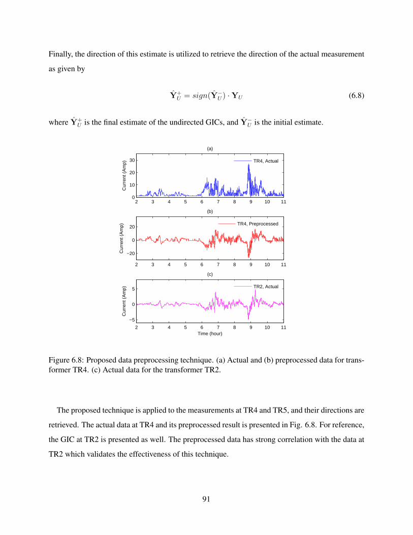
Finally, the direction of this estimate is utilized to retrieve the direction of the actual measurement
as given by
Y+U = sign(Y−U ) ·YU (6.8)
where Y+U is the final estimate of the undirected GICs, and Y−U is the initial estimate.
2 3 4 5 6 7 8 9 10 110
10
20
30
Cur
rent
(A
mp)
(a)
TR4, Actual
2 3 4 5 6 7 8 9 10 11
−20
0
20
Cur
rent
(A
mp)
(b)
TR4, Preprocessed
2 3 4 5 6 7 8 9 10 11
−5
0
5
Time (hour)
Cur
rent
(A
mp)
(c)
TR2, Actual
Figure 6.8: Proposed data preprocessing technique. (a) Actual and (b) preprocessed data for trans-former TR4. (c) Actual data for the transformer TR2.
The proposed technique is applied to the measurements at TR4 and TR5, and their directions are
retrieved. The actual data at TR4 and its preprocessed result is presented in Fig. 6.8. For reference,
the GIC at TR2 is presented as well. The preprocessed data has strong correlation with the data at
TR2 which validates the effectiveness of this technique.
91

Table 6.3: Grounding Resistance and Coefficients of Investigated ATC Transformers
Name HE HN Rg
TR1 20.816 25.831 0.168TR2 21.5 34.4 0.222TR3 -13.8 4.2 0.168TR4 -14.875 18.818 0.181TR5 3.2 2.14 0.148
6.5.2 GIC Model Validation
To perform the GIC model validation, first the transformers coefficients are calculated. The in-
vestigated transformers are part of the Eastern Interconnect (EI). The EI system is simulated in
PowerWorld Simulator using the available network parameters and the coefficients are calculated
based on the method described earlier. Unfortunately, the grounding resistances are not available
for the EI system and a simplistic model was used to estimate their values. The assumed grounding
resistances and the resulting coefficients are presented in Table 6.3.
In theory, all parts of the network should be considered for calculating the coefficients. However,
studies show that the GIC impacts are localized and considering only the nearby areas provides
sufficient accuracy. In the current study, all the EI areas are included in the calculations, yet
later investigations demonstrated that this was not necessary and considering only the areas near
Wisconsin provided sufficient accuracy.
There are two GIC models to be validated: The conventional model in (3.14) and the modified
one in (6.2) with the introduced scales. The model validation framework is used to evaluate the
effectiveness of these models through real data analysis.
Figure 6.9 illustrates how well each individual measurement agrees with the conventional model.
First, the E-field is estimated from the GIC measurements through the conventional model as
proposed in (10.2). The estimated E-field is multiplied by the transformer coefficients to get the
estimated GIC using I = HE. This estimation is then compared with the actual measurement.
According to the figure, the estimated and actual GICs agree very well at TR2, TR3, and TR4. The
estimate at TR1 does not agree well with the actual GIC, but still has the same order of magnitude.
The worst agreement is at TR5 where the estimate is almost zero, even though the actual GIC
92
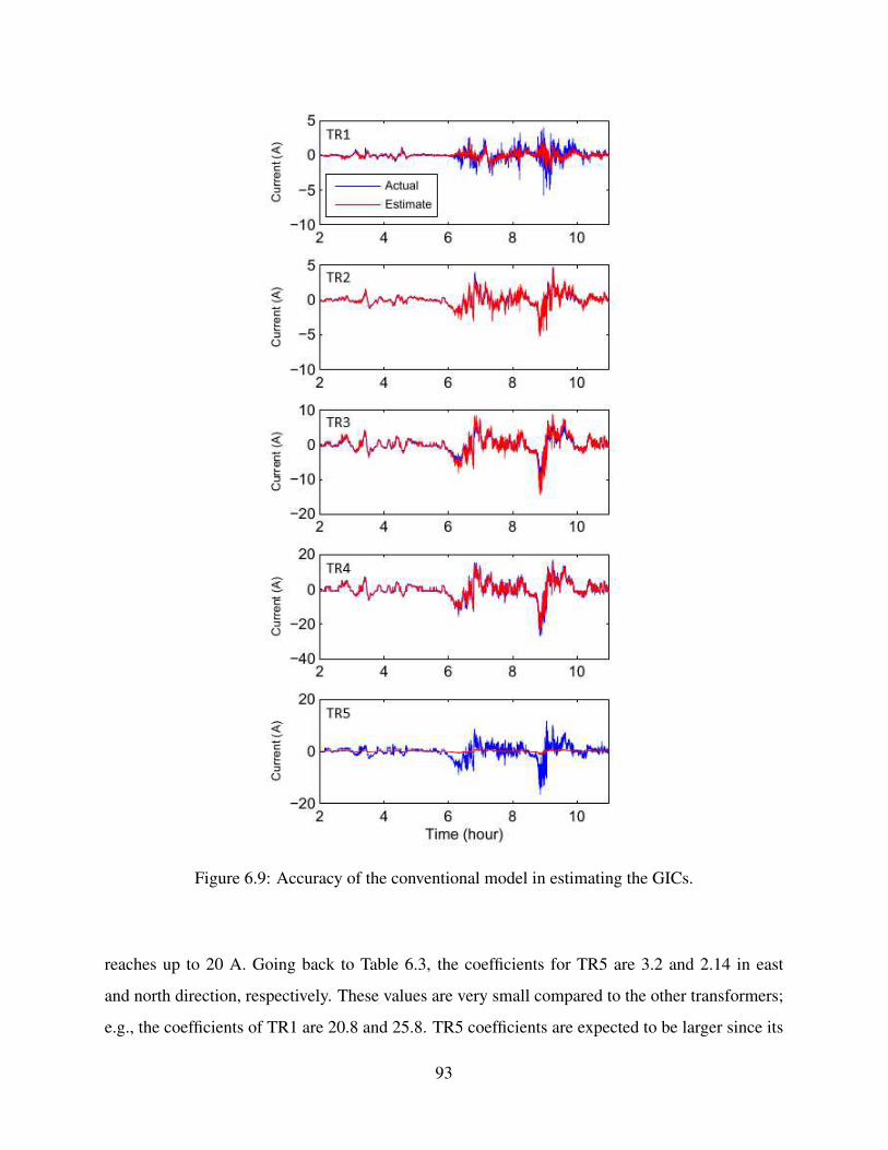
Figure 6.9: Accuracy of the conventional model in estimating the GICs.
reaches up to 20 A. Going back to Table 6.3, the coefficients for TR5 are 3.2 and 2.14 in east
and north direction, respectively. These values are very small compared to the other transformers;
e.g., the coefficients of TR1 are 20.8 and 25.8. TR5 coefficients are expected to be larger since its
93

Table 6.4: Pearson Correlation Coefficients Between the GICs
Name TR1 TR2 TR3 TR4 TR5TR1 1 -0.166 0.072 0.117 0.051TR2 -0.166 1 0.791 0.652 0.651TR3 0.072 0.791 1 0.700 0.653TR4 0.117 0.652 0.700 1 0.883TR5 0.051 0.651 0.653 0.883 1
measured GIC is in the same order as the other transformers. This casts doubt on the accuracy of
the assumed coefficients. The modified model may be used to correct the inaccurate coefficients
through the scales as will be demonstrated shortly.
The modified model accounts for the system uncertainties and in particular, the inaccurate co-
efficients. Figure 6.10 compares the estimated GICs obtained from the modified model with the
actual measurements. This time, the estimated GIC at TR5 has high agreement with the actual
one, which confirms that the modified model accounts for the inaccurate coefficients by assigning
a larger scale to TR5. Another interesting observation is that the estimated GIC at TR1 is close
to zero. This is because the modified model assigns a very small scale to TR1 which reduces the
estimated GIC to almost zero. Recall that the modified model assigns zero scales to the outlier
measurements as was demonstrated through an example in previous section (see Fig. 6.3). Similar
to the example case, the measurement at TR1 has irregularity, and hence gets a zero scale. It is
clear in Fig. 6.10 that all the measurements are correlated except for TR1. This can be confirmed
using the Pearson correlation coefficients as presented in Table 6.4. The value at row TRX and
column TRY of the table is the coefficient between the GICs at transformers X and Y . Pairwise
comparison of these coefficients confirms the weak correlation for TR1.
Many factors could contribute to zeroing out the scale of a transformer. One possible reason is
having a different E-field than the rest of the network, in which case the uniform E-filed assumption
does not hold and the GIC model is no longer valid. Hence, the transformer with a different E-field
is excluded from the model by setting its scale to be zero. TR1 is located in the northern part of
Michigan and is on the shore of Lake Superior as shown in Fig. 6.6. Its higher latitude as well as
the nearby body of water could result in a different E-field and eventually zero out the scale.
94
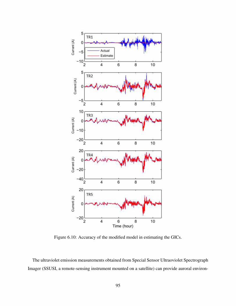
Figure 6.10: Accuracy of the modified model in estimating the GICs.
The ultraviolet emission measurements obtained from Special Sensor Ultraoviolet Spectrograph
Imager (SSUSI, a remote-sensing instrument mounted on a satellite) can provide auroral environ-
95

Table 6.5: Accuracy Comparison of the E-field Estimation Techniques for the ATC system
Estimation Technique Eastward Field Northward FieldProposed 0.629 0.740Conventional 0.656 0.737SVD 0.630 0.016
mental data records (EDRs) with information on the electron energy flux (Q), the magnetic field
lines and the auroral boundaries during a solar storm [91]. Analysis of the auroral EDRs for the
March 9, 2012, storm indicates that the aurora moved to the lower latitudes during the storm.
The aurora even hit the Ottawa magnetic observatory as confirmed with its magnetic field mea-
surements. This suggests that the irregularity at TR1 could be due to the magnetic disturbances
associated with the aurora. Further exploration into the E-field at the transformer TR1 and why its
scale vanishes will be an interesting future study.
The performance of the proposed technique is compared with the SVD-based approach. The
E-field estimated from the magnetic data is compared with the estimate from GIC measurements
using both methods, and their Pearson correlation coefficients are presented in Table 6.5. For ref-
erence, the results for the conventional GIC model in (3.14) are also included in the table. All three
methods estimate the eastward E-field quite accurately with their correlation coefficients around
0.6. The proposed model and the conventional one estimate the northward E-field with relatively
good accuracy, whereas the estimate from the SVD-based approach is extremely inaccurate with
its correlation coefficient equal to 0.016.
Figure 6.11 presents the eastward E-field obtained from the magnetic data as compared with the
estimate from the GIC measurements using both the proposed model and the SVD analysis. The
fields are scaled to have unit Euclidean norm. The estimate from both methods agrees well with
that from the magnetic data. Figure 6.12 demonstrates a similar comparison for the E-field in the
north direction. In this direction, the estimate from the proposed model agrees relatively well with
that from the magnetic data, whereas the estimate from SVD analysis has significant mismatches.
For better clarity, the estimate from the conventional model is not included in Fig. 6.4 and Fig. 6.5
as it is perfectly aligned with the estimate from the proposed model.
96
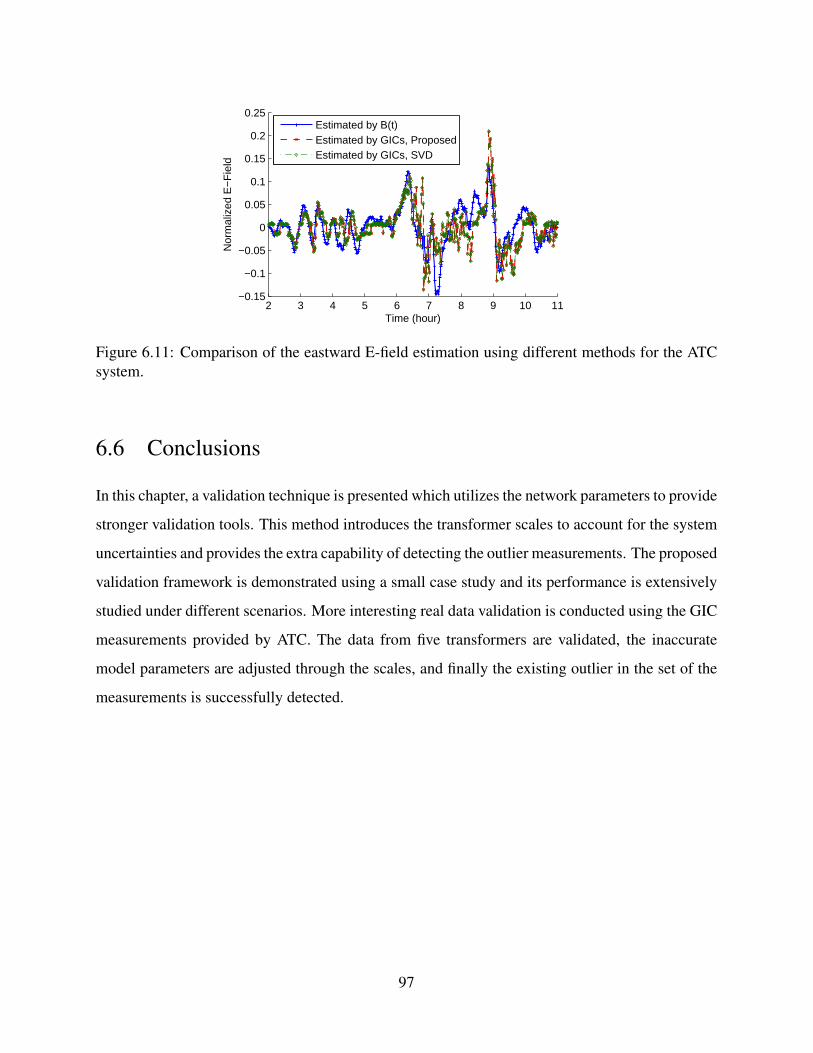
2 3 4 5 6 7 8 9 10 11−0.15
−0.1
−0.05
0
0.05
0.1
0.15
0.2
0.25
Time (hour)
Nor
mal
ized
E−
Fie
ld
Estimated by B(t)Estimated by GICs, ProposedEstimated by GICs, SVD
Figure 6.11: Comparison of the eastward E-field estimation using different methods for the ATCsystem.
6.6 Conclusions
In this chapter, a validation technique is presented which utilizes the network parameters to provide
stronger validation tools. This method introduces the transformer scales to account for the system
uncertainties and provides the extra capability of detecting the outlier measurements. The proposed
validation framework is demonstrated using a small case study and its performance is extensively
studied under different scenarios. More interesting real data validation is conducted using the GIC
measurements provided by ATC. The data from five transformers are validated, the inaccurate
model parameters are adjusted through the scales, and finally the existing outlier in the set of the
measurements is successfully detected.
97

2 3 4 5 6 7 8 9 10 11−0.2
−0.1
0
0.1
0.2
0.3
0.4
0.5
Time (hour)
Nor
mal
ized
E−
Fie
ld
Estimated by B(t)Estimated by GICs, ProposedEstimated by GICs, SVD
Figure 6.12: Comparison of the northward E-field estimation using different methods for the ATCsystem.
98
CHAPTER 7
SUBSTATION GROUNDING RESISTANCEESTIMATION FOR IMPROVED GMD MODELVALIDATION
7.1 Introduction
This chapter focuses on estimating the substation grounding resistance to improve the modeling
of geomagnetically induced currents (GICs). Grounding resistances are not included in the stan-
dard power flow models, and their approximate values are often used for performing GIC studies.
This chapter provides an algorithm to estimate the resistances from the GIC measurements. This
algorithm calculates the linear sensitivity factors of the GICs around the local grounding resistive
components and uses linear regression to solve for the resistances. The effectiveness of the pro-
posed algorithm is demonstrated using both a small test case as well as a 62500-bus model of the
North American Eastern Interconnection. The proposed technique reduces the uncertainties of the
GMD model by providing more accurate grounding resistances. This improves the resiliency to
GMDs through better assessment of the GICs and their risks.
The chapter is organized as follow: The algorithm for estimating the substation grounding resis-
tance through GIC measurements is presented in Section 7.2. In Section 7.3, the dependency of the
proposed technique on the E-field is identified and proper adjustments are considered to eliminate
such dependencies. Section 7.4 discusses the practical issues with implementing the algorithm and
a suitable framework is presented which simplifies the implementation. Section 7.5 demonstrates
the proposed technique using a 20-bus test case, while the application on a large 62500-bus system
is given in Section 7.6. Section 7.7 presents a conclusion and directions for future work.
99

7.2 Grounding Resistance Estimation
The grounding resistance error is described as the vector of the differences between the actual
grounding resistances and the assumed ones as given by
∂R = R −R0 (7.1)
where R is the vector containing the actual grounding resistance of all the substations and R0 is
the vector of the assumed grounding resistances.
The sensitivity of the GIC to the grounding resistance is defined as the percent variation of the
current in terms of the percent variation of the grounding resistance as given by [45]:
sij =∂(%IGIC,i)
∂(%Rj)=
(∂IGIC,i/IGIC,i)
(∂Rj/Rj)(7.2)
In this study, the actual variation is used instead of the percent variation to simplify the problem
formulation: sij = ∂IGIC,i/∂Rj . For a set of K substations, one can build the K ×K sensitivity
matrix S = sij where sij is the sensitivity of the GIC at substation i to the grounding resistance
of substation j. The sensitivity depends on the E-field direction and the sensitivity matrix is de-
fined for a particular direction. Let SN and SE denote the sensitivity matrices for northward and
eastward E-fields. The grounding resistance error modifies the coefficient matrix by HN ← HN + SN∂R
HE ← HE + SE∂R(7.3)
Substituting the updated coefficient matrix in the GIC model gives rise to
[(HN + SN∂R) | (HE + SE∂R)]× E = Y (7.4)
Defining the matrix Yb := HE, (7.4) can be rewritten as:
(EE ⊗ SE + EN ⊗ SN)T∂R = vec(Y −Yb) (7.5)
100

where ⊗ is the Kronecker product and vec() is the vectorization function. Defining the matrix
A := (EE ⊗ SE + EN ⊗ SN)T generates an overdetermined system with ∂R as the unknown:
A∂R = vec(Y −Yb) (7.6)
Least squares estimation can be used to estimate ∂R as given by
∂RLS
: = arg min∂R‖vec(Y −Yb)−A∂R‖2
= (ATA)−1ATvec(Y −Yb) (7.7)
The coefficient modification presented in (7.3) is valid only for small values of ∂R as the sen-
sitivities are linear approximations. However, ∂R may be large when the grounding resistance
data is inaccurate or unavailable. To tackle this, the process can be performed iteratively until ∂R
converges to zero. The resistances obtained at each iteration are used as the initial values for the
consecutive iteration. The steps of this iterative algorithm are described in Algorithm 7.
Algorithm 7 Grounding Resistance Estimation with E-field1: procedure GROUNDING RESISTANCE ESTIMATION WITH E-FIELD(Y, X, R0)2: Initialize the estimated resistances R to R0
3: Define the convergence tolerance, ε4: Initialize ∂R to the all-ones vector5: while | ∂R |> ε do6: Calculate the sensitivities SN and SE
7: Calculate Yb = HE8: Calculate A = (EE ⊗ SE + EN ⊗ SN)T
9: Solve for ∂R through ∂R = (ATA)−1ATvec(Y −Yb)10: Update the resistances by R = R + ∂R11: end while12: return R13: end procedure
The inputs of the algorithm are the GIC measurements Y, the E-field E and the available
grounding resistances R0. If no resistance data is available, R0 is represented by a vector of
random values within the range of 0.05 and 0.3 (reasonable range for the grounding resistance).
The output of the algorithm is R, which is the vector of estimated grounding resistances.
101

In theory, the estimated resistance obtained from the proposed technique is the same as the one
measured by the conventional methods. The proposed algorithm serves as an alternative solution
when measuring the resistances is not feasible for practical reasons. There are several challenges
associated with the measurement-based approaches. First, external objects such as water pipeline
and adjacent railroad tracks distort the earth potential contours. Second, sources of dc current such
as dc railroad tracks, pipelines cathodic protection systems and dc transmission lines produce stray
currents which interfere with the grounding resistance measurements. Third, the resistance of the
electrodes used for the measurements can introduce error if the substation being tested has low
resistivity. Last, the grounding resistance mostly depends on the humidity, salt level or temper-
ature and therefore is time-variant and may change significantly with seasons. The conventional
grounding resistance measurements are usually performed every five to ten years and even the
most recent one might not capture the current state of the soil regarding its humidity, salt level or
temperature. In contrast, the estimate from the GIC measurements is in semi-real time. Motivated
by the negative impacts of GMDs, electric utilities are investing in GIC monitoring enhancement.
More GIC sensors are being installed in the grid which widens the applications of the proposed
technique.
7.2.1 Sensitivity Calculation
The algorithm presented earlier requires calculation of the sensitivity matrices at each iteration.
There are analytical techniques to derive the sensitivities as functions of the network parame-
ters [45]. Alternatively, one can follow the sensitivity definition to calculate the sensitivities as
described in Algorithm 8. The algorithm takes the grounding resistances as input. This allows
calculating the sensitivities in each iteration after the grounding resistances are updated.
7.3 Dependency on the Electric Field
The problem with the proposed technique is that it depends on the E-field whereas only the GIC
data is assumed to be available, not the E-field. To address this issue, first, the E-field is esti-
mated through the GICs and then is used in the algorithm. Since the grounding resistances are
102

Algorithm 8 Sensitivity Calculation1: procedure SENSITIVITY CALCULATION(R)2: Initialize the grounding resistances to R3: Enforce an eastward E-field to get IE0.4: Enforce a northward E-field to get IN0.5: for n = 1 to n <K do6: Increase the resistance of substation n by 10%.7: Enforce an eastward E-field to get IE .8: Enforce a northward E-field to get IN .9: Calculate the nth column of the northward sensitivity matrix by SEn =
10(IE − IE0)/IE0
10: Calculate the nth column of the northward sensitivity matrix by SNn = 10(IN −IN0)/IN0
11: Set the resistance of substation n back to default.12: end for13: return SN and SE
14: end procedure
not available in the beginning and are going to be estimated later, a meaningful E-field estimation
should be robust to the grounding resistance error. The appendix demonstrates that the ordinary
LS method can successfully estimate the E-field up to scaling even when the grounding resistances
are inaccurate:
ELS := arg minE‖Y −HE‖2 = (HTH)−1HTY (7.8)
This estimation scales with the actual E-field, but the ratio is unknown. This uncertainty is included
in the model through:
E = αE⇒ α vec(Yb) + A∂R = vec(Y) (7.9)
where α is the unknown ratio between the estimated E-field and the actual one. Yb is similar to
Yb except that the estimated E-field is used in its definition instead of the actual one: Yb = HE.
The system is augmented to include α as an additional unknown:
[A | vec(Yb)] ×
∂R
α
= vec(Y) (7.10)
103

Defining xa := [∂R | α]T as the augmented state and Aa := [A | vec(Yb)] as the augmented
design matrix, least squares can be used to solve for ∂R and α as given by
xLSa : = arg minxa
‖vec(Y)−Aaxa‖2
= (ATaAa)
−1ATa vec(Y) (7.11)
Least squares provides the solution with the minimum Euclidean norm. However, it is better to
minimize the Euclidean norm of ∂R, but allow α to take any value. To find the solution with this
particular property, regularized least squares may be used as described in the following.
7.3.1 Regularized Least Squares
Ordinary least squares is the standard approach to solve the overdetermined system of equation
Mx = b (7.12)
where the sum of the squared residuals ‖Mx − b‖2 is minimized. Regularized least squares give
preference to a particular solution with desirable properties by adding the regularization term as
expressed by
x := arg minx‖Mx− b‖2 + µ‖Fx‖2 (7.13)
where F is suitably chosen to capture the desired regularization and µ is the penalty weight [92].
This forms a multi-objective optimization problem and its closed-form solution is given by
x = (MTM + µFTF)−1MT b (7.14)
For the augmented system in (7.10), it is desired to enforce ∂R to zero, but leave α unconstrained.
This can be done by selecting F as a diagonal matrix with 1 on all its diagonal entries but the last
104

one as given by
F = diag([~1(1,S), 0]) (7.15)
where S is the number of substations. The algorithm for estimating the grounding resistance when
the E-field is not available is summarized in the following:
Algorithm 9 Grounding Resistance Estimation without E-field1: procedure GROUNDING RESISTANCE ESTIMATION WITHOUT E-FIELD(Y, R0)2: Initialize the grounding resistances R to R0
3: Estimate the E-field by E = (HTH)−1HTY4: Define the convergence tolerance, ε5: Initialize ∂R to the all-ones vector6: while | ∂R |> ε do7: Calculate the sensitivities SN and SE
8: Calculate Yb := HE9: Calculate Aa := [(EE ⊗ SE + EN ⊗ SN)T | vec(Yb)]
10: Solve for ∂R by [∂R | α]T = (ATaAa)
−1ATa vec(Y)
11: Update the resistances by R = R + ∂R12: end while13: return R14: end procedure
7.4 Algorithm Implementation
To implement the algorithm efficiently, parts of the computations are performed in a computation
program like MATLAB and the rest in a commercial power system software like PowerWorld
Simulator. The process involves repetitively running simulation in the power system software,
collecting data and transferring it to the computation program for further analysis. With the actual
algorithm, the intercommunication between the two programs is as follows: Store the grounding
resistances in the computation program, simulate the network with the current resistances in the
power system software, calculate the sensitivities, transfer to the computation program and calcu-
late the new grounding resistances accordingly. Repeat the process until the grounding resistances
converge. This process is illustrated in Fig. 7.1.
105
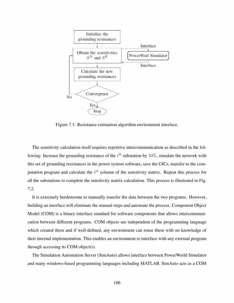
Figure 7.1: Resistance estimation algorithm environment interface.
The sensitivity calculation itself requires repetitive intercommunication as described in the fol-
lowing: Increase the grounding resistance of the ith substation by 10%, simulate the network with
this set of grounding resistances in the power system software, save the GICs, transfer to the com-
putation program and calculate the ith column of the sensitivity matrix. Repeat this process for
all the substations to complete the sensitivity matrix calculation. This process is illustrated in Fig.
7.2.
It is extremely burdensome to manually transfer the data between the two programs. However,
building an interface will eliminate the manual steps and automate the process. Component Object
Model (COM) is a binary-interface standard for software components that allows intercommuni-
cation between different programs. COM objects are independent of the programming language
which created them and if well-defined, any environment can reuse them with no knowledge of
their internal implementation. This enables an environment to interface with any external program
through accessing its COM object(s).
The Simulation Automation Server (SimAuto) allows interface between PowerWorld Simulator
and many windows-based programming languages including MATLAB. SimAuto acts as a COM
106
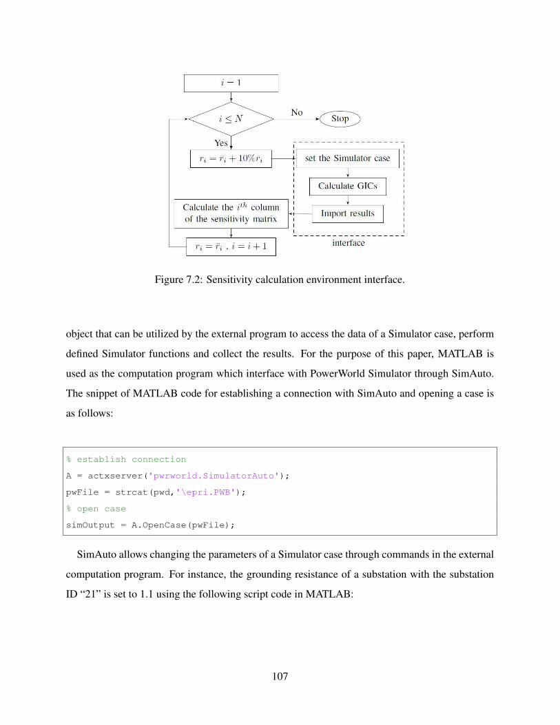
Figure 7.2: Sensitivity calculation environment interface.
object that can be utilized by the external program to access the data of a Simulator case, perform
defined Simulator functions and collect the results. For the purpose of this paper, MATLAB is
used as the computation program which interface with PowerWorld Simulator through SimAuto.
The snippet of MATLAB code for establishing a connection with SimAuto and opening a case is
as follows:
% establish connection
A = actxserver('pwrworld.SimulatorAuto');
pwFile = strcat(pwd,'\epri.PWB');
% open case
simOutput = A.OpenCase(pwFile);
SimAuto allows changing the parameters of a Simulator case through commands in the external
computation program. For instance, the grounding resistance of a substation with the substation
ID “21” is set to 1.1 using the following script code in MATLAB:
107

% change grounding resistance
type = 'Substation';
fields = 'SubNum','GICSubGroundOhms';
values = 21,1.1;
simOutput = serv.ChangeParametersSingleElement ...
(type, fields, values);
SimAuto also offers the capability to execute Simulator functions through the external software.
For example, the script code below enforces an E-field with unity magnitude and 90 degree direc-
tion to the simulator case and solves the GIC flow:
% calculate GIC
fileline = 'GICCalculate(1,90,NO)';
After changing the grounding resistance and calculating the GICs, it is desired to transfer the
results from PowerWorld to MATLAB. Below is an example of importing the neutral current for
the transformer between buses 17 and 18:
% transfer GIC
type = 'Transformer';
fields = 'BusNum','BusNum:1','LineCircuit',...
'GICXFNeutralAmps';
output = serv.RunScriptCommand(fileline);
values = 17,18,1,1;
simOutput = serv.GetParametersSingleElement ...
(type,fields,values);
It is necessary that all the commands are defined properly and without any ambiguity. For example,
to import the neutral current of a transformer, defining only the connecting buses is not enough if
there is more than one transformer between those two buses. The line circuit should be specified
as well in order to uniquely identify the transformer.
108

Table 7.1: Grounding Resistances of the 20-bus Test Case
Name Actual Resistance Assumed Resistance Error (%)SUB1 0.20 0.31 53.53SUB2 0.20 0.14 31.21SUB3 0.20 0.26 27.72SUB4 1.00 0.90 9.56SUB5 0.10 0.03 70.00SUB6 0.10 0.17 72.83SUB7 0.10 0.16 61.87
7.5 Numerical Results Using a Small Test Case
The effectiveness of the proposed method is validated though simulation. The 20-bus system in
[38] is investigated. The substation grounding resistances are presented in Table 7.1. These values
are not available to the algorithm and need to be estimated. Instead, the assumed resistances listed
in the table are provided. The assumed grounding resistances have an average of 136% absolute
error with the error defined as
ErrorRg =‖R0 −R‖2‖R‖2
(7.16)
Synthetic GIC data is created by enforcing an E-field to the system and obtaining the induced
GICs through solving the GIC flow in PowerWorld Simulator. For the purpose of this study, the
E-field measured during an actual geomagnetic storm is used to maximize the likeness to real GIC
measurements [81]. The E-field collected at Fredericksburg observatory during the March 9, 2012
storm is investigated. Fredericksburg observatory is located in the US at a latitude/longitude of
38.205N , 77.373W . To simulate the system perturbation and measurement noise, white Gaus-
sian noise with different signal-noise-ratios (SNRs) is added to the ideal GICs and the synthetic
measurements are obtained.
First, the substation grounding resistances are estimated assuming the E-field is known using
Algorithm 7. Figure 7.3 illustrates the estimation error when the GIC measurements are subject to
different levels of Gaussian noise. It is observed that the algorithm converges after two iterations
109

1 2 3 4 5 6 70
20
40
60
80
100
120
140
Iteration
Err
or N
orm
(%
)%33.9
%19.2%14.7
%0.8 %0.0
SNR= 5SNR= 10SNR= 20SNR= 40SNR=100
Figure 7.3: Estimation error for the test case when the E-field is known.
for all the noise levels. The final estimation error which is obtained after convergence depends
on the noise level; i.e., higher noise level results in higher estimation error. For example, the
estimation error is 33.9% when the SNR is 5 dB and zero when SNR is 100 dB (almost noise-
free).
Sometimes, the E-field is not provided to the algorithm and only the GICs are available. In
this case, the algorithm first estimates the E-field based on the GICs and then uses this estimation
to find the resistances as presented in Algorithm 9. This technique is implemented for different
measurement noise levels as illustrated in Fig. 7.4. The y-axis in the figure has a logarithmic scale.
It is observed that the algorithm diverges when the SNR is 20 dB or lower (higher noise level).
For the SNR equal to 30 dB, the algorithm converges, but the estimation accuracy is not much
improved from the initial guess; 136.9% error in the initial guess is reduced only to 79.2% which
is still too high. The estimation error drops significantly for lower noise levels with the estimation
error equal to 8.7%, 0.5% and zero for SNRs equal to 40 dB, 50 dB and 100 dB, respectively.
Comparing these results with those from Fig. 7.3, one can conclude that the algorithm is more
robust to measurement noise when the E-field is available. Moreover, the algorithm has a faster
convergence rate when the E-field is available as it converges in only two iterations with the E-field
as opposed to three to four iterations without the E-field.
In practice, the GICs are not available at all the substations and only few substations have GIC
sensors installed at their transformer neutrals. Hence, it is desired to evaluate the algorithm when
110

1 2 3 4 5 6 710
−4
10−2
100
102
104
106
Iteration
Err
or N
orm
(%
)
%39326.4
%79.2
%8.7
%0.5
%0.0
SNR= 20
SNR= 30
SNR= 40
SNR= 50
SNR=100
Figure 7.4: Estimation error for the test case when the E-field is unknown.
the GIC data is sparse. To model this, only the GICs at substations 1, 2, and 3 are provided to
the algorithm and the rest are unknown. In this case, the algorithm reduces the GIC model to
include only the substations with available data and ignores the rest of the network. Using the
reduced model, the algorithm performs similarly to the normal case, but finds only the resistance
of the substations included in the model. First, the substations are estimated assuming the E-field
is known as illustrated in Fig. 7.5. For all noise levels, the error decreases after each iteration
until it converges to around 10% at the third iteration. The interesting observation is that the
algorithm is extremely robust to the measurement noise under this scenario and the curves for
different noise levels are almost aligned. The other observation is that unlike the previous cases,
the estimation error does not converge to zero when the measurements are noise free. This is
because some of the substations have inaccurate grounding resistances and yet no GIC sensors
which makes it impossible to track down the error they introduce to the estimation and makes the
system unobservable. Simulation results indicate that the estimation error reduces to zero when
the grounding resistances of the substations that are missing GIC sensors are accurate and the GIC
measurements are noise free. The more substations with missing GIC sensors in the system and
the more inaccurate their assumed grounding resistance, the higher the estimation error as verified
through simulation.
It is important to realize that even though the algorithm may not provide 100% accuracy all
the time, its estimation is remarkably better than the initial values. In other words, the algorithm
111

1 2 3 4 5 6 70
20
40
60
80
100
120
140
Iteration
Err
or N
orm
(%
)
%128.6
%16.5
%9.0 %10.6 %10.4 %10.5
SNR= 5SNR= 10SNR= 20SNR= 40SNR=100
Figure 7.5: Estimation error for the test case when the E-field is known and the GIC data is sparse.
Table 7.2: Estimated Resistances for the Test Case When the GIC Data is Sparse
Name R R0Initial
Error (%) REstimationError (%)
SUB1 0.20 0.36 81.15 0.19 4.41SUB2 0.20 0.24 18.86 0.20 2.32SUB3 0.20 0.40 97.91 0.22 9.28
does not find the actual resistances, but it moves toward them and converges to somewhere in their
close proximity. This is demonstrated in Table 7.2 by comparing the actual resistances with the
estimated ones when the GIC measurements are noise free. For reference, the initial grounding
resistances are presented as well.
The next validation test is to study the performance of the algorithm when the E-field is not
available and the GIC data is sparse. The GICs at the first three substations (1, 2 and 3) are
provided, but the E-field and the rest of GICs are missing. The algorithm excludes the substations
with missing GICs from the model, estimates the E-field from the available GICs with one level of
ambiguity and finally uses regularized least squares to find the resistances. Figure 7.6 illustrates
the estimation error under this scenario for different measurement noise levels. The algorithm
diverges when the SNR is 10 dB or lower. The algorithm converges for lower noise levels with the
estimation error equal to 22.9%, 17.4% and 17.8% for SNRs equal to 10, 40 and 100, respectively.
112
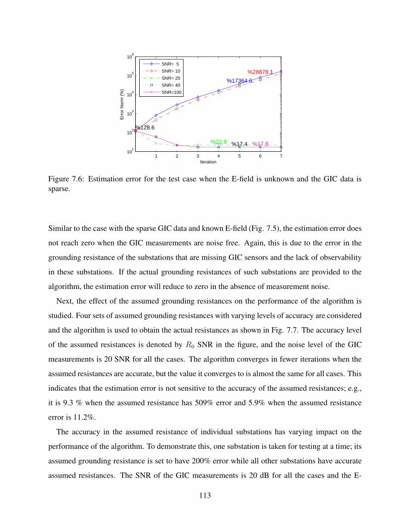
1 2 3 4 5 6 710
1
102
103
104
105
106
Iteration
Err
or N
orm
(%
)%128.6
%17364.6
%28878.1
%22.9 %17.4 %17.8
SNR= 5
SNR= 10
SNR= 20
SNR= 40
SNR=100
Figure 7.6: Estimation error for the test case when the E-field is unknown and the GIC data issparse.
Similar to the case with the sparse GIC data and known E-field (Fig. 7.5), the estimation error does
not reach zero when the GIC measurements are noise free. Again, this is due to the error in the
grounding resistance of the substations that are missing GIC sensors and the lack of observability
in these substations. If the actual grounding resistances of such substations are provided to the
algorithm, the estimation error will reduce to zero in the absence of measurement noise.
Next, the effect of the assumed grounding resistances on the performance of the algorithm is
studied. Four sets of assumed grounding resistances with varying levels of accuracy are considered
and the algorithm is used to obtain the actual resistances as shown in Fig. 7.7. The accuracy level
of the assumed resistances is denoted by R0 SNR in the figure, and the noise level of the GIC
measurements is 20 SNR for all the cases. The algorithm converges in fewer iterations when the
assumed resistances are accurate, but the value it converges to is almost the same for all cases. This
indicates that the estimation error is not sensitive to the accuracy of the assumed resistances; e.g.,
it is 9.3 % when the assumed resistance has 509% error and 5.9% when the assumed resistance
error is 11.2%.
The accuracy in the assumed resistance of individual substations has varying impact on the
performance of the algorithm. To demonstrate this, one substation is taken for testing at a time; its
assumed grounding resistance is set to have 200% error while all other substations have accurate
assumed resistances. The SNR of the GIC measurements is 20 dB for all the cases and the E-
113
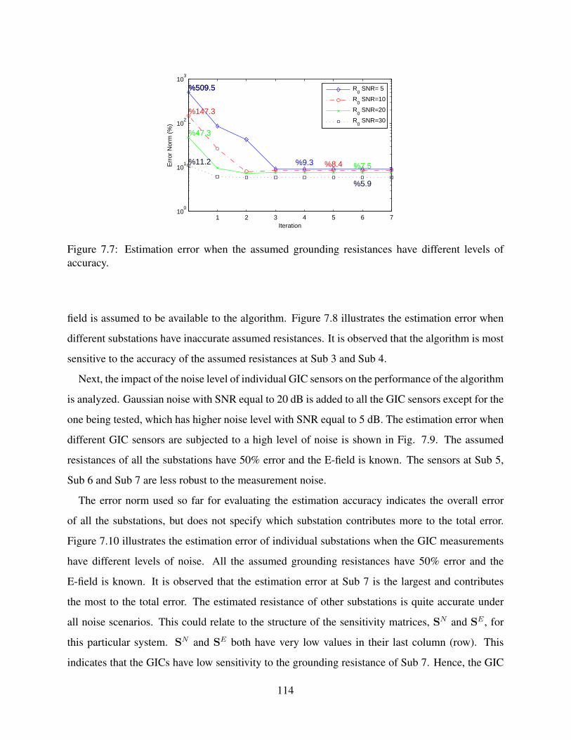
1 2 3 4 5 6 710
0
101
102
103
Iteration
Err
or N
orm
(%
)
%509.5%509.5
%9.3
%147.3
%8.4
%47.3
%7.5%11.2
%5.9
R
0 SNR= 5
R0 SNR=10
R0 SNR=20
R0 SNR=30
Figure 7.7: Estimation error when the assumed grounding resistances have different levels ofaccuracy.
field is assumed to be available to the algorithm. Figure 7.8 illustrates the estimation error when
different substations have inaccurate assumed resistances. It is observed that the algorithm is most
sensitive to the accuracy of the assumed resistances at Sub 3 and Sub 4.
Next, the impact of the noise level of individual GIC sensors on the performance of the algorithm
is analyzed. Gaussian noise with SNR equal to 20 dB is added to all the GIC sensors except for the
one being tested, which has higher noise level with SNR equal to 5 dB. The estimation error when
different GIC sensors are subjected to a high level of noise is shown in Fig. 7.9. The assumed
resistances of all the substations have 50% error and the E-field is known. The sensors at Sub 5,
Sub 6 and Sub 7 are less robust to the measurement noise.
The error norm used so far for evaluating the estimation accuracy indicates the overall error
of all the substations, but does not specify which substation contributes more to the total error.
Figure 7.10 illustrates the estimation error of individual substations when the GIC measurements
have different levels of noise. All the assumed grounding resistances have 50% error and the
E-field is known. It is observed that the estimation error at Sub 7 is the largest and contributes
the most to the total error. The estimated resistance of other substations is quite accurate under
all noise scenarios. This could relate to the structure of the sensitivity matrices, SN and SE , for
this particular system. SN and SE both have very low values in their last column (row). This
indicates that the GICs have low sensitivity to the grounding resistance of Sub 7. Hence, the GIC
114

0 1 2 3 4 5 6 7 8 90
50
100
150
200
250
300
350
400
Iteration
Err
or N
orm
(%
)
Sub1Sub2Sub3Sub4Sub5Sub6Sub7
Figure 7.8: Estimation error when different substations have inaccurate assumed resistances.
measurements provide little observability to its resistance. The algorithm is generally not accurate
in estimating the resistance of the substations with low sensitivities; however, it is still effective in
improving the GIC calculation since such substations have low impact on the GICs regardless of
their resistance values.
7.6 Application of the Algorithm to Larger Systems
The algorithm is applied to a 62,500 bus, 27,600 substation model of the Eastern Interconnection
used in [37]. The goal is to estimate the grounding resistance of the EI substations that are more
critical to the GMD analysis and whose values might be of greater interest to utilities. High voltage
transformers are more susceptible to GMDs and the existing GIC sensors already installed by
utilities are often at such transformers. Motivated by this, the list of high voltage transformers in
the EI system is considered. This includes more than 200 transformers with a high-side voltage
greater than 300 kV. Next, the top 100 transformers in the list which are most affected by GMDs are
identified. This is done by calculating the GICs on the transformers under typical E-field profiles
(northward and eastward field with unity magnitude) and selecting those with higher average GICs.
A substation might have multiple transformers with high GICs in which case only one of the
transformers is selected to avoid redundancy.
115

0 1 2 3 4 5 6 7 8 90
20
40
60
80
100
120
140
Iteration
Err
or N
orm
(%
)
Sub1Sub2Sub3Sub4Sub5Sub6Sub7
Figure 7.9: The estimation error when different GIC sensors are subject to high level of noise.
The same E-field data used for the 20-bus system is used here, i.e. the data for the March 9,
2012, storm measured at Fredericksburg observatory. This E-field is enforced to the system and
the induced GICs are calculated. White Gaussian noise with 30 dB SNR is added to the ideal GICs
and the synthetic measurements are obtained.
The assumed grounding resistances of the 100 investigated substations are generated by adding
noise with SNR equal to 10 to the actual resistances. Figure 7.11 presents the actual and the
assumed resistances (iteration 0); the former is to be estimated by the algorithm and the latter is
provided as the initial guess. Starting with the assumed resistances, the algorithm moves towards
the actual resistances as shown in the figure (iteration 1 and 2). The E-field is assumed to be
unknown for this experiment. The estimation error over the first iterations is calculated and it is
observed that the error reduces from 120% to zero in three iterations.
Note that the actual resistances used for the EI system are fictitious and do not reflect the actual
values of the real system. As was mentioned before, the grounding resistances are seldom available
and this is also the case for the EI system. The proposed algorithm can find the actual resistance
of an EI substation if its GIC measurement ever becomes available. On another note, the line and
transformer resistances, and the network topology, used in the study are obtained from the EI power
flow model with good accuracy, and the grounding resistance is the only piece of information
which is missing in the model.
116

5.52 3.72 2.07 1.35
6.48 3.87 1.96 1.39
4.18 2.59 1.23 0.83
3.09 1.53 0.90
5.44 2.92 1.69 0.83
3.86 1.84 1.01
32.49 17.98 10.67 5.33 1.92
GIC SNR
Sub
stat
ion
Inde
x
5 10 15 20 30 40
1
2
3
4
5
6
7
5
10
15
20
25
30
Figure 7.10: Estimation error of individual substations when the GIC measurements have differentlevels of noise.
7.7 Conclusion
In this chapter, an analytical technique is developed which derives the substation grounding re-
sistances from the GIC measurements. In this technique, the relation between the GICs and the
grounding resistances is linearized through some sensitivity parameters and linear regression is
used to solve for the resistances. The uncertainty in the grounding resistances introduces error to
the parameters of the linear model. To tackle this, the problem is reformulated to decouple the
uncertainties from the known parameters and regularized least squares is used for solving it. The
effectiveness of the algorithm is evaluated using both a small test case as well as a 62,500 bus
model of the EI system. As demonstrated, the algorithm can estimate the grounding resistances
accurately even when the available GIC measurements are sparse and the assumed resistances have
large error.
The study suggests several directions for future research. First, the proposed algorithm should
be applied to real GIC measurements as opposed to synthetic ones used here and its robustness
to actual measurement noise and uncertainty needs to be validated. Second, the algorithm can
be integrated into GIC model validation framework for improved performance. The grounding
117
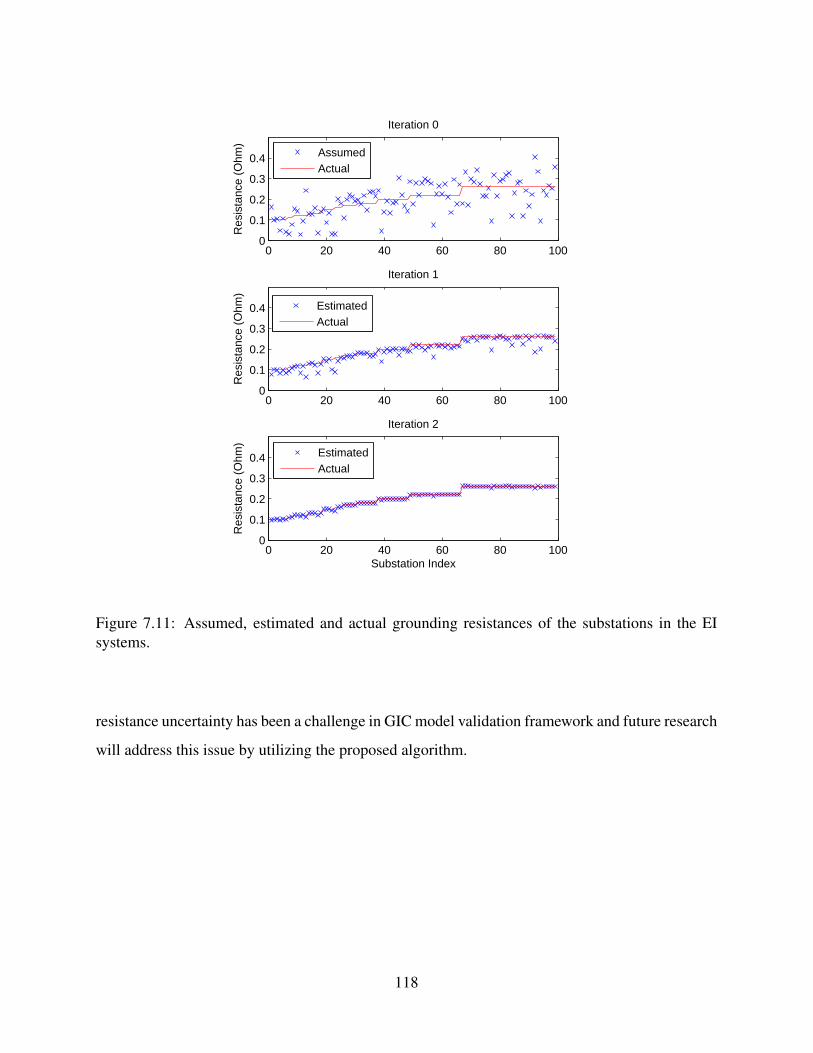
0 20 40 60 80 1000
0.1
0.2
0.3
0.4
Res
ista
nce
(Ohm
)
Iteration 0
AssumedActual
0 20 40 60 80 1000
0.1
0.2
0.3
0.4
Res
ista
nce
(Ohm
)
Iteration 1
EstimatedActual
0 20 40 60 80 1000
0.1
0.2
0.3
0.4
Substation Index
Res
ista
nce
(Ohm
)
Iteration 2
EstimatedActual
Figure 7.11: Assumed, estimated and actual grounding resistances of the substations in the EIsystems.
resistance uncertainty has been a challenge in GIC model validation framework and future research
will address this issue by utilizing the proposed algorithm.
118

CHAPTER 8
ENHANCED MAGNETIC FIELD ESTIMATION
8.1 Introduction
This chapter focuses on interpolating the magnetic field data to improve the GIC model validation.
The available magnetic data is very sparse over the Earth’s surface and readings of a distant mag-
netometer are often used for model validation. This chapter proposes an interpolation technique
that considers the magnetic field inherent characteristics. The real magnetic data over a three-year
period is analyzed and the dependencies between the observatories are extracted. These interde-
pendencies are eventually incorporated in the interpolation and higher performance is achieved.
The techniques in [52, 53] utilize the physics of the Earth’s magnetic field to improve the inter-
polation. This chapter approaches the problem differently. The historical magnetic data collected
over time is extensively analyzed to capture interesting information which can eventually improve
the interpolation. Correlation analysis is performed to extract the hidden dependencies between
the magnetic fields of different observatories. Such dependencies are later utilized to improve the
interpolation accuracy. Finally, the correlation analysis is extended to the frequency domain using
dynamic wavelet transform.
This work is motivated by the research presented in Chapters 5 and 6 which looked at correlating
the GICs on transformer neutral measurements in Wisconsin for the March 9, 2012, storm. The
closest magnetometers to Wisconsin are FRD (Fredericksburg, VA) and OTT (Ottawa, ON), which
are still more than 800 miles away. The results of this work tend to facilitate such GIC validation
framework by providing the interpolated magnetic field across the Wisconsin area.
The chapter is organized as follows: The dataset used for this study is described in Section
8.2. The correlation analysis is the subject of Section 8.3, which explores the possible interde-
pendencies between the observatories. The proposed interpolation technique incorporating the
119

dependencies is presented in Section 8.4, while real data analysis is used in Section 8.5 to evaluate
its performance. In Section 8.6, the correlation analysis is extended to frequency domain using
wavelet transform. Section 8.7 presents a conclusion and directions for future work.
8.2 The investigated Magnetic Data
This study uses the 1-minute ground magnetometer data for a three-year test period from January
1, 2011 to December 30, 2014. The data is collected from 21 observatories in North America with
the geographic locations illustrated in Fig. 3.2. USGS provides this data in a daily format in [81].
The test data includes 1095 datasets where each dataset has the daily data of all the observatories.
The magnetic data is in three directions – north, east and vertical. The field variation in the
vertical direction does not impact the power system significantly. Hence, only the north and east
directions are considered for this study. The data analysis and interpolation techniques can be
performed in each direction separately and independently. To be concise, the analysis is performed
only in the north direction throughout the chapter and readers can extend it to the east direction
using the same procedure.
The raw data is preprocessed before performing any analysis. First, the missing data is identified
and effectively removed from the raw data. Second, the median filter is used to remove the spikes
and unwanted transients. Last, the representation of the magnetic data is transformed from polar
to Cartesian coordinates and the fields in the north and east directions are obtained.
8.3 Correlation Analysis
The correlation between the magnetic fields of different observatories may reveal interesting in-
formation about the evolution of the magnetic field over the Earth’s surface during a storm. In this
section, correlation analysis is performed on the three-year data and various visualization tools are
developed to understand the pairwise correlations between the observatories.
The average dependency between two observatories is obtained by first calculating the correla-
tion coefficient between their magnetic data during each day and then taking the average over all
120
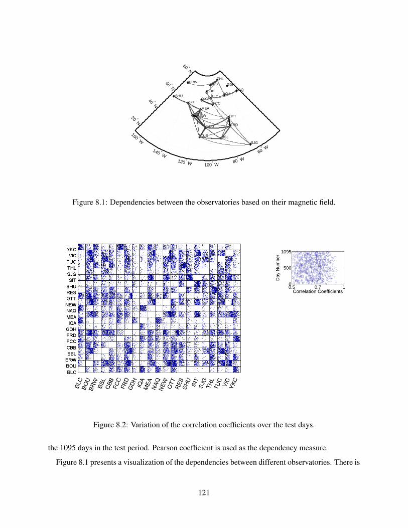
BLC
BOU
BRW
BSL
CBB
FCC
FRD
GDH
IQA
MEA
NAQ
NEW OTT
RES
SHU
SIT
SJG
THL
TUC
VIC
YKC
160 ° W
140 ° W
120 ° W 100° W 80° W
60° W
20 ° N
40 ° N
60 ° N
80 ° N
Figure 8.1: Dependencies between the observatories based on their magnetic field.
0.5 0.7 10
500
1095
Day
Num
ber
Correlation Coefficients
Figure 8.2: Variation of the correlation coefficients over the test days.
the 1095 days in the test period. Pearson coefficient is used as the dependency measure.
Figure 8.1 presents a visualization of the dependencies between different observatories. There is
121

a line connecting two observatories if their average correlation coefficient is greater than 0.5. The
thickness and color of the connecting line relates to the coefficient value where higher coefficients
have thicker lines with darker shades of grey.
The variation of the correlation coefficients over the test days is visualized in Fig. 8.2. Each
block corresponds to one pair of observatories with the observatory codes shown in the vertical
and horizontal axes. Here, only the coefficients more than 0.5 are visualized. For each block, the
horizontal axis is used to visualize the coefficient value ranging from 0.5 to 1. The vertical axis
denotes the day number in the study period (ranging from 1 to 1095). As an example, the block
corresponding to the pair of MEA (Meanook, AB) and SIT (Sitka, AK) observatories is magnified
in the figure.
It is observed that some blocks contain a large number of points while others are sparsely cov-
ered. A block is densely covered when its corresponding observatories are highly dependent and
their coefficients are greater than 0.5 on most of the days. Such observatory pairs are referred to
as dependent observatories. The other interesting observation is that at some blocks, the points are
concentrated around one line, while at others they are scattered all over the area. An example of
the former is the block for the FRD and OTT pair, while the MEA-SIT block follows the latter.
Probability distribution may be used to better demonstrate this aspect. The probability distribution
of the coefficients between FRD and OTT is illustrated in Fig. 8.3. For this pair, the coefficients
have a small standard deviation with a peak at around 0.95. This indicates that for an unseen data,
one can tell the value of the coefficient between FRD and OTT with high confidence.
The probability distribution for the SIT and MEA pair is illustrated in Fig. 8.4. Unlike the
previous pair, this one exhibits a wide range of variation in its coefficients. Hence, for an unseen
datum, one can tell these observatories are dependent with high confidence. However, the value of
their coefficient remains unknown.
The probabilistic visualization of the dependent observatories is presented in Fig. 8.5. Each
colored block corresponds to one pair of observatories with the observatory codes shown in the
vertical and horizontal axes. The number in each block indicates the probability that the corre-
sponding observatories are dependent. This probability is obtained by counting the number of
days when the correlation coefficient is greater than 0.5 and dividing it by the total number of days
(1095 for this study). The probabilities are expressed in percentage and the block colors correlate
122

0 0.2 0.4 0.6 0.8 10
0.1
0.2
0.3
0.4
0.5
0.6
0.7
Correlation Coefficient
Pro
babi
lity
FRD−OTT
Figure 8.3: Probability distribution of the correlation coefficients (FRD-OTT pair).
0 0.2 0.4 0.6 0.8 10
0.02
0.04
0.06
0.08
0.1
0.12
Correlation Coefficient
Pro
babi
lity
SIT−MEA
Figure 8.4: Probability distribution of the correlation coefficients (SIT-MEA pair).
with their values. Probabilities less than 40% are not visualized in this figure.
8.4 MultiVariant Interpolation
Given the known points yi = y(xi) for i = 1, · · · , N , inverse distance weighting (IDW) may be
used to obtain the interpolated value y at a given point x as expressed in:
y(x) =
∑Ni=1 ωi(x)yi∑Ni=1 ωi(x)
(8.1)
123
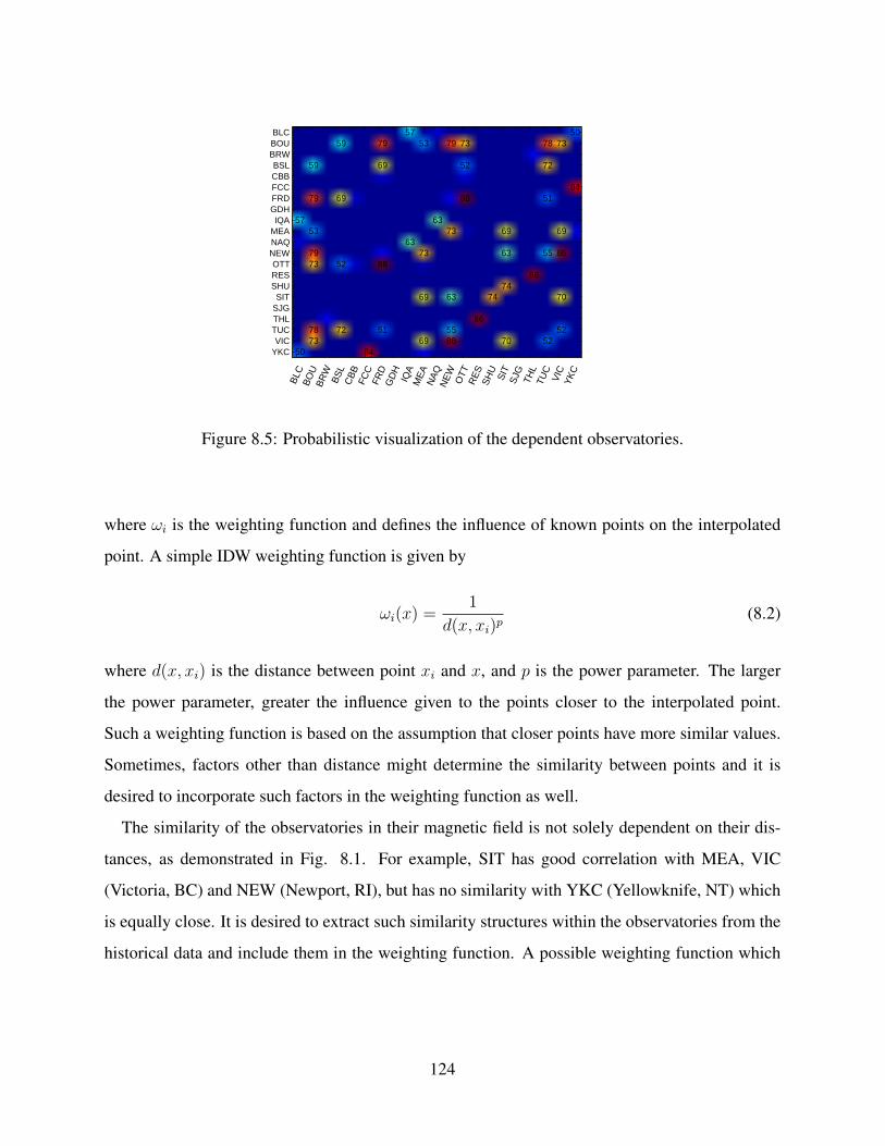
57
50
59
79
53
7973
7873
59
69
52
72
84
79
69
88
51
57
63
53
73
69
69
63
79
73
63
5586
73
52
88
86
74
69
63
74
70
86
78
72
51
55
52
73
69
86
70
52
50
84
BLC
BO
UB
RW
BS
LC
BB
FCC
FRD
GD
HIQ
AM
EA
NA
QN
EW
OTT
RE
SS
HU
SIT
SJG TH
LTU
CV
ICY
KC
BLCBOUBRWBSLCBBFCCFRDGDHIQA
MEANAQNEWOTTRESSHUSIT
SJGTHLTUCVIC
YKC
Figure 8.5: Probabilistic visualization of the dependent observatories.
where ωi is the weighting function and defines the influence of known points on the interpolated
point. A simple IDW weighting function is given by
ωi(x) =1
d(x, xi)p(8.2)
where d(x, xi) is the distance between point xi and x, and p is the power parameter. The larger
the power parameter, greater the influence given to the points closer to the interpolated point.
Such a weighting function is based on the assumption that closer points have more similar values.
Sometimes, factors other than distance might determine the similarity between points and it is
desired to incorporate such factors in the weighting function as well.
The similarity of the observatories in their magnetic field is not solely dependent on their dis-
tances, as demonstrated in Fig. 8.1. For example, SIT has good correlation with MEA, VIC
(Victoria, BC) and NEW (Newport, RI), but has no similarity with YKC (Yellowknife, NT) which
is equally close. It is desired to extract such similarity structures within the observatories from the
historical data and include them in the weighting function. A possible weighting function which
124

BLC
BOU
BRW
BSL
CBB
FCC
FRD
GDH
IQA
MEA
NAQ
NEW OTT
RES
SHU
SIT
SJG
THL
TUC
VIC
YKC
160 ° W
140 ° W
120 ° W 100° W 80° W
60° W
20 ° N
40 ° N
60 ° N
80 ° N
Figure 8.6: A visualization of the similarity parameters.
incorporates the similarity structures is given by:
ωi(x) =c(x, xi)
d(x, xi)(8.3)
where c(x, xi) is a binary variable called similarity parameter that specifies the similarity between
points x and xi as expressed in
c(x, xi) :=
1, x and xi are similar
0, otherwise(8.4)
The similarity parameters are obtained from the three-year data and based on the dependency
probabilities presented in Fig. 8.5. The similarity parameter between two observatories is one
when their dependency probability is more than 50% and zero otherwise. A visualization of these
parameters is presented in Fig. 8.6. There is a line connecting two observatories when their
similarity parameter is one.
125

0 5 10 15 202.088
2.09
2.092
2.094
2.096x 10
4
Time (hour)
Bx
(nT
)
Actual
Interpolate
Figure 8.7: Comparison of the interpolated and actual field at FRD for a quiet day, March 1, 2012.
8.5 Real Data Studies
In this section, the performance of the proposed interpolation is evaluated. Assuming N observa-
tories with known magnetic field, one observatory is selected for testing and the fields at the N −1
remaining observatories are used to interpolate its value. Comparing the interpolated field with the
actual one yields the accuracy. This procedure is referred to as the N-1 accuracy test.
The accuracy in interpolating the magnetic field at FRD is demonstrated in Fig. 8.7. The mag-
netic field from March 1, 2012, is used for this testing. The fields at the remaining observatories
are used to interpolate the FRD value. The similarity parameters obtained from the three-year test
period are incorporated in the interpolation to achieve higher accuracy. Clearly, the interpolated
field agrees well with the actual one.
The accuracy in interpolating FRD field during a stormy day is illustrated in Fig. 8.8. The mag-
netic field from the March 9, 2012, storm is used for this testing. It is observed that the accuracy
is lower for the stormy day than the quiet day. Note that this observation is specific to this study
and may not be generally true. For example, the interpolation accuracy for FCC (Fort Churchill,
MB) during the same storm is demonstrated in Fig. 8.9. For this observatory, the interpolation has
extremely high accuracy even during the storm. To understand how the interpolation performance
relates to the level of the geomagnetic activity, more thorough analysis is required which is left for
future work.
Next, the N-1 accuracy test is performed on all the observatories and for all the days in the
126

0 5 10 15 202.06
2.07
2.08
2.09
2.1x 10
4
Time (hour)
Bx
(nT
)
Actual
Interpolate
Figure 8.8: Comparison of the interpolated and actual field at FRD for the March 9, 2012 storm.
0 5 10 15 207500
8000
8500
9000
9500
10000
Time (hour)
Bx
(nT
)
Actual
Interpolate
Figure 8.9: Comparison of the interpolated and actual field at FCC for the March 9th, 2012 storm.
test period. For each test, one observatory and one day is selected. The field at the selected
observatory during the selected day is interpolated using the fields at the remaining observatories.
The agreement between the interpolated and the actual field is quantified by:
Error(%) = 100× ‖Y − Y ‖2‖Y ‖2
(8.5)
where Y and Y are the vectors of the actual and interpolated magnetic fields, respectively, and ‖·‖2denotes the Euclidean norm. Using this error definition, the average interpolation error is visual-
ized in Fig. 8.10. For each observatory, first the interpolation error is obtained for all the 1095 days
in the test period and then their average is calculated. For reference, the dependencies between the
observatories are also illustrated using the visualization in Fig. 8.1. The interesting observation
127

BLC
BOU
BRW
BSL
CBB
FCC
FRD
GDH
IQA
MEA
NAQ
NEW OTT
RES
SHUSIT
SJG
THL
TUC
VIC
YKC
160 ° W
140 ° W 120 ° W 100° W 80
° W 60° W
20 ° N 40 ° N
60 ° N 80 ° N
30
40
50
60
70
80
90
Figure 8.10: Average interpolation error at different observatories.
is that the interpolation error is lower at the observatories which have higher dependencies with
others. For example, MEA, NEW, BOU and BUC are highly interdependent as demonstrated by
the thick, dark lines connecting them. They also have lower interpolation error as shown with the
blue area in the figure.
Integrating the similarity parameters into the interpolation improves the accuracy. Figure 8.11
presents the average interpolation error when no prior information about the similarities is avail-
able. The weighting function in (8.2) is used for this study which is solely dependent on the
distances. Note that the color bar in the figure ranges from 82% to 94%. This error reduces to 30%
when the similarity parameters are included, as shown in Fig. 8.10. It is important to mention that
the error definition used here results in relatively high values even for accurate interpolations and
is only suitable for comparison purposes. For example, the interpolations presented in Fig. 8.7 and
Fig. 8.8 have errors of 19.4% and 89.4%, respectively.
8.6 Wavelet Analysis
Wavelet transform decomposes a signal into different frequency bandwidths while maintaining
the temporal structure of the signal. Unlike Fourier transform that is only localized in frequency,
wavelets are localized in both time and frequency. Wavelets provide a combination of time and
frequency spectrum, but the frequency spectrum is not as detailed as that obtained from the Fourier
128

BLC
BOU
BRW
BSL
CBB
FCC
FRD
GDH
IQA
MEA
NAQ
NEW OTT
RES
SHUSIT
SJG
THL
TUC
VIC
YKC
160 ° W
140 ° W 120 ° W 100° W 80
° W 60° W
20 ° N 40 ° N
60 ° N 80 ° N
82
84
86
88
90
92
94
Figure 8.11: Average interpolation error when the similarity parameters are not integrated.
Figure 8.12: Three-level wavelet decomposition.
transform.
The signal is decomposed into two frequency bandwidths, namely approximation and detail.
The approximation signal contains the lower half of the frequencies while the detail includes the
high half. This process could be repeated on the approximation signal to achieve higher orders of
wavelet decomposition. A diagram of the three-level decomposition is presented in Fig. 8.12. In
the figure, Di and Ai are, respectively, the detail and approximation signals at level i, and X is the
input signal. The detail signal at each level provides a temporal representation of the input signal
within a certain frequency bandwidth. The frequency bandwidth associated with each level for a
three-level decomposition is illustrated in Fig. 8.13.
Wavelet analysis is applied to the magnetic field data to understand the interdependencies be-
129

Figure 8.13: Frequency bandwidths of different components in a three-level wavelet decomposi-tion.
Table 8.1: The Frequency Bands of the Detail Signals Using 1-second Magnetic Data
Wavelet Detail Frequency (MHz)D1 500-1000D2 250-500D3 125-250D4 62.5-125
tween the observatories with respect to their frequency spectrum [51]. In this analysis, 1-second
magnetic data is used instead of the 1-minute data to cover a wider frequency range. Wavelet de-
composition is performed on the data up to 15 levels. The detail signal at each level is used as a
temporal representation of its corresponding frequency band. The bands covered by D1 to D4 are
presented in Table 8.1.
Next, the correlation analysis is performed on different frequency bands. The correlation coeffi-
cients are calculated between the detail signals of the same level, but different observatories. The
coefficients between three sets of observatory pairs at different frequency bands are plotted in Fig.
8.14. The magnetic field from the March 9, 2012, storm is used for this testing. The interesting
observation is that the coefficients are higher at the lower frequencies bands. This implies that the
low frequency components of the magnetic field have higher correlation with their counterparts at
the other observatories.
130

Figure 8.14: Correlation coefficient at different frequency bands.
8.7 Conclusion
In this chapter, the magnetic field measurements at 21 observatories in North America over a
three-year period are extensively studied and various statistical measures are extracted from the
data. Correlation analysis is performed to capture the possible dependencies between the observa-
tories. It is observed that the magnetic fields at some observatories are highly correlated and this
dependency is not always related to their distance. To address this, the inverse distance weighting
interpolation is modified to account for such dependencies. The modified interpolation improves
over the conventional one as demonstrated through real data analysis. Finally, the correlation anal-
ysis is extended to the frequency domain using the wavelet transform. The interpolation technique
developed in this chapter can provide a more accurate magnetic field input for the GMD model
validation frameworks presented in Chapter 5 and Chapter 6. This improves their validation capa-
bility and makes them stronger tools for enhancing power system resiliency.
131
CHAPTER 9
ENHANCED E-FIELD ESTIMATION THROUGHDYNAMIC MODELING AND FILTERING
9.1 Introduction
This chapter presents dynamic modeling of the electric field as an effective technique to improve
the E-field estimation. Actual magnetic field measurements during several GMD events are used
to develop a practical dynamic model for the electric field. The developed dynamic model is in-
tegrated into a Kalman filter and higher accuracy in E-field estimation is achieved. The overall
performance of the proposed estimation technique over the conventional LS estimation is demon-
strated through simulation.
The improved E-field estimation developed in this chapter can facilitate the GMD model vali-
dation frameworks in Chapters 5 and 6. GIC measurements are often subject to different types of
noise, and using Kalman filtering instead of the investigated LS estimator makes these validation
techniques more robust to such measurement uncertainties.
The rest of the chapter is organized as follows: The dynamic modeling for E-field is introduced
in Section 9.2. Section 9.3 presents Kalman filtering and its application in E-field estimation. In
Section 9.4, real E-field data is used to analyze the dynamics of the E-field and derive its dynamic
model. A comparison between the Kalman filter approach and the LS estimator is performed in
Section 9.5, while Section 9.6 presents a conclusion and directions for future work.
9.2 Dynamic Modeling of Electric Field
Analyzing the variation of the E-field with time, one can recognize the correlation of the data with
its previous values. This phenomenon is verified by calculating the autocorrelation of the E-field
as illustrated in Fig. 9.1. The geomagnetic data at Fredericksburg observatory during the day of
132
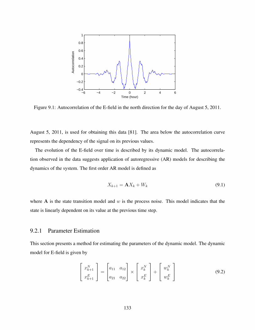
−6 −4 −2 0 2 4 6−0.4
−0.2
0
0.2
0.4
0.6
0.8
1
Time (hour)
Aut
ocor
rela
tion
Figure 9.1: Autocorrelation of the E-field in the north direction for the day of August 5, 2011.
August 5, 2011, is used for obtaining this data [81]. The area below the autocorrelation curve
represents the dependency of the signal on its previous values.
The evolution of the E-field over time is described by its dynamic model. The autocorrela-
tion observed in the data suggests application of autoregressive (AR) models for describing the
dynamics of the system. The first order AR model is defined as
Xk+1 = AXk +Wk (9.1)
where A is the state transition model and w is the process noise. This model indicates that the
state is linearly dependent on its value at the previous time step.
9.2.1 Parameter Estimation
This section presents a method for estimating the parameters of the dynamic model. The dynamic
model for E-field is given by xNk+1
xEk+1
=
a11 a12
a21 a22
× xNk
xEk
+
wNk
wEk
(9.2)
133

where wN = N (0, σ2N) and wE = N (0, σ2
E). For this model, the state transition model is a 2× 2
matrix which has four unknown parameters. The process noise is a 2-dimensional random vector
with normal distribution and the variance of each dimension should be estimated. To estimate
these six unknown parameters, the problem is formulated as a linear regression problem and the
LS estimation is used for solving it.
The data forN consecutive time steps are used to estimate the parameters of the dynamic model.
Writing the dynamic model at all the time steps gives rise to n−1 equations. These n−1 equations
are stacked together and written in vector form as
X =M× A+ W
X =[xN2 , x
N3 , · · · , xNn , xE2 , xE3 , · · · , xEn
]TW =
[wN1 , w
N2 , · · · , wNn−1, wE1 , wE2 , · · · , wEn−1
]TA =
[a11, a12, a21, a22
]T
M =
xN1
xN2...
xNn−1
xE1
xE2...
xEn−1
0...
0
0...
0
0...
0
0...
0
xN1
xN2...
xNn−1
xE1
xE2...
xEn−1
(9.3)
The LS estimation is used to solve the overdetermined system of equations presented in (9.3).
The parameters of the state transition model are calculated by
A = (MTM)−1MT X (9.4)
134

and the variance vector of the process noise is given by
W =
WN
WE
= X− AM⇒
σN = Var(WN
)σE = Var
(WE
) (9.5)
9.2.2 Simplified Dynamic Model
The dynamic model presented in (9.1) assumes a coupling between the northward and eastward
fields. This allows values in one direction to be dependent on the previous values in other direc-
tions. One can simplify the dynamic model by ignoring this coupling. The simplified model is
given by xNk+1 = aNxNk + wNk
xEk+1 = aExEk + wEk
(9.6)
where aN and aE are the transition models for the northward and eastward E-fields respectively.
The method for estimating these two parameters is similar to the one presented in the previous
section.
9.3 E-field Estimation Using Kalman Filter
A stochastic linear time-invariant (LTI) system consists of the dynamic model and the observer
model as presented in (9.7). The dynamic model describes the evolution of the state with time and
is in the form of an ordinary differential equation. The observer model relates the observations to
the states through a linear model. In equation (9.7), Wk and Vk are independent Gaussian random
vectors and they represent the state noise and the observation noise respectively. Xk+1 = AXk +Wk
Zk = HXk + Vk(9.7)
To solve the stochastic LTI system, the classical Kaman filter is used. The Kalman filter is a
135
recursive estimator which estimates the state at the current step based on the state estimated at
the previous step and the current observations. The estimation process is usually presented in two
steps: the prediction step and the correction step. In the prediction step, the estimated state at the
previous step is used to make a prior estimate of the state at the current step as given by
X−k = AX+k−1 (9.8)
where X−k is the priori estimate at the kth time step and X+k−1 is the posteriori estimate or the final
estimate at the k − 1th time step. The prediction step also involves estimating the error covariance
at the current step based on the error covariance at the previous step as described in (9.9). In this
equation, Q is the covariance of the noise for the state model.
P−k = AP+k−1A
T + Q (9.9)
In the correction step, the prior estimate of the state is corrected by utilizing the observation at
the current step as given by
X+k = X−k + Kk(Xk −HX−k ) (9.10)
where Kk is the Kalman gain at the k-th step and is calculated by (9.11). The Kalman gain is the
optimal weighting for the innovation Zk −HXk and minimizes the error.
Kk = P−k HT (HP−k HT + R)−1 (9.11)
Finally, the error covariance is updated at the end of the correction step as given by
P+k = (I−KkH)P−k (9.12)
The prediction step and the correction step are executed recursively until the states at all the time
steps are estimated. To initialize the recursions, the estimated state and its error covariance at the
136

first time step are initialized by X0 = E[X0]
P0 = E[(X0 − µ)(X0 − µ)T ](9.13)
If the initial state is known, X0 = X0 and P0 = 0 are used instead for the initialization.
9.4 E-field Dynamic Modeling Using Real Data
In this section, actual magnetic field measurements are used to study the dynamic behavior of the
E-field during geomagnetic storms. During the day of August 5, 2011, a geomagnetic storm started
at 18:00 UTC and reached a very high level in the following hours. The magnetic field measured
at Fredericksburg observatory during this storm is used to obtain the E-field as illustrated in Fig.
9.2. Note that the variation of E-field is very small during the normal hours, but large peaks are
observed during the storm. A dynamic model is developed for the data during the storm. The
parameters of this model are calculated by eqs. (9.3) to (9.5). These parameters are a11 = 0.923,
a12 = 0.621, a21 = 0.009, a22 = 0.866, σN = 11.24, and σE = 2.55. Note that σE is remarkably
smaller than σN , which indicates that the autocorrelation of electric field in the east direction is
more significant.
The dynamic model can be simplified by ignoring the coupling between the northward and
eastward E-fields as proposed by (9.6). The parameters of the simplified model are aN = 0.923,
aE = 0.866, σN = 11.24, and σE = 2.55. Interestingly, the noise level of the simplified model is
equal to the original model. This indicates that the simplified model is as accurate as the original
model and ignoring the coupling between the two fields introduces no error to the model. In other
words, the coupling is insignificant and can be ignored for simplification purposes. Hence, the
simplified dynamic model will be used for the ensuing numerical analysis.
It is important to understand how the parameters of the dynamic model change over different
storms. The E-field data for three different geomagnetic storms and three normal days are analyzed
and the parameters of their dynamic models are calculated as presented in Table 9.1. An interesting
observation is that the noise level for stormy days is higher than for normal days. This implies that
137

0 5 10 15 20−60
−40
−20
0
20
40
← Storm →← Normal →
Time (hour)
E−
field
(m
V/k
m)
Northward
(a)
0 1 2 3 4 5 6 7 8 9−2
−1.5
−1
−0.5
0
0.5
1
Time (hour)
Nor
mal
ized
E−
Fie
ld
Magnetic Field
GICs, SVD
GICs, Modified Model
(b)
Figure 9.2: E-field in (a) north direction and (b) east direction.
the dynamic model has lower accuracy in modeling the E-field of a stormy day compared to a
normal day.
Note that the values of aN and aE range only from 0.80 to 0.93 for both stormy days and
normal days. This suggests that these parameters are not highly dependent on the individual E-
field measurements and could be approximated as constants over different sets of data. According
to Table 9.1, the average of aN over the six datasets is 0.88 and the average of aE is also 0.88. These
two values can be used as the approximation of the dynamic model parameters for any given E-
field data. The advantage of this approximation is that one can develop the dynamic model for
unknown datasets.
138
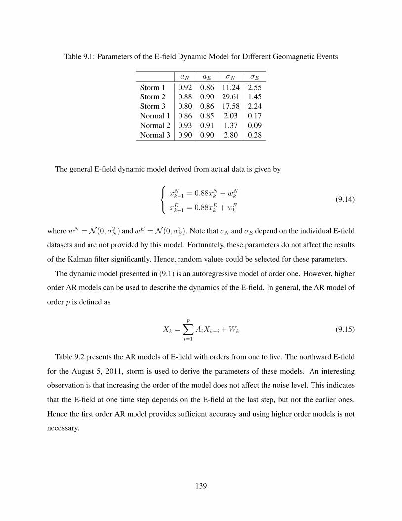
Table 9.1: Parameters of the E-field Dynamic Model for Different Geomagnetic Events
aN aE σN σE
Storm 1 0.92 0.86 11.24 2.55Storm 2 0.88 0.90 29.61 1.45Storm 3 0.80 0.86 17.58 2.24Normal 1 0.86 0.85 2.03 0.17Normal 2 0.93 0.91 1.37 0.09Normal 3 0.90 0.90 2.80 0.28
The general E-field dynamic model derived from actual data is given by xNk+1 = 0.88xNk + wNk
xEk+1 = 0.88xEk + wEk
(9.14)
wherewN = N (0, σ2N) andwE = N (0, σ2
E). Note that σN and σE depend on the individual E-field
datasets and are not provided by this model. Fortunately, these parameters do not affect the results
of the Kalman filter significantly. Hence, random values could be selected for these parameters.
The dynamic model presented in (9.1) is an autoregressive model of order one. However, higher
order AR models can be used to describe the dynamics of the E-field. In general, the AR model of
order p is defined as
Xk =
p∑i=1
AiXk−i +Wk (9.15)
Table 9.2 presents the AR models of E-field with orders from one to five. The northward E-field
for the August 5, 2011, storm is used to derive the parameters of these models. An interesting
observation is that increasing the order of the model does not affect the noise level. This indicates
that the E-field at one time step depends on the E-field at the last step, but not the earlier ones.
Hence the first order AR model provides sufficient accuracy and using higher order models is not
necessary.
139

Table 9.2: Parameters of the AR Models with Different Orders
Order Transition Model Noise1 a1 =0.92, σ =11.22 a1 =1.02, a2 =-0.10 σ =11.23 a1 =1.04, a2 =-0.32, a3 =0.21 σ =11.24 a1 =1.05, a2 = -0.33, a3 =0.26, a4 =-0.04, σ =11.25 a1 = 1.05, a2 =-.35, a3 =.27, a4 =-.09, a4 =.04 σ =11.2
9.5 Numerical Results and Simulations
In this section, the performance of the LS estimator is compared with the Kalman filter based on
the simulation results. The effect of sensor failure rate, outlier rate and Gaussian noise level on the
performance of the two estimators is studied and accuracy comparison is conducted accordingly.
For this study, the 20-bus system in [38] is investigated.
To analyze the performance of the estimators, the E-field presented in Fig. 9.2 is enforced to
the system. The GICs induced by this E-field are determined via solving the GIC flow program
in PowerWorld Simulator. The GIC model in (3.14) can also be used for calculating transformer
GICs. The results obtained from this model are identical to those provided by the GIC flow pro-
gram.
The GICs obtained from the GIC flow program represent ideal measurements. The noisy mea-
surements are obtained by adding white Gaussian or nonuniform noise to the ideal GIC values. The
Monte Carlo simulation with 1000 realizations is used to simulate the randomness in the additive
noise.
The effect of the Gaussian noise level on the performance of the estimators is illustrated in Fig.
9.3. In this calculation, the outlier rate and failure rate are set to zero. According to this figure, the
Kalman filter outperforms the LS method at higher noise levels and falls below the LS method at
lower noise levels. Moreover, the advantage of the Kalman filter over the LS method is more for
the east direction. This relates to the higher autocorrelation of the E-field in the east direction as
was mentioned earlier.
Figure 9.4 illustrates the effect of the outlier rate on the performance of the estimators. In this
study, the Gaussian noise level and failure rate are set to zero. The Kalman filter outperforms the
140
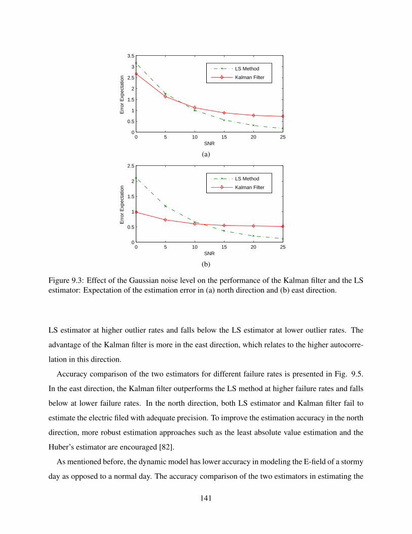
0 5 10 15 20 250
0.5
1
1.5
2
2.5
3
3.5
SNR
Err
or E
xpec
tatio
n
LS Method
Kalman Filter
(a)
0 5 10 15 20 250
0.5
1
1.5
2
2.5
SNR
Err
or E
xpec
tatio
n
LS Method
Kalman Filter
(b)
Figure 9.3: Effect of the Gaussian noise level on the performance of the Kalman filter and the LSestimator: Expectation of the estimation error in (a) north direction and (b) east direction.
LS estimator at higher outlier rates and falls below the LS estimator at lower outlier rates. The
advantage of the Kalman filter is more in the east direction, which relates to the higher autocorre-
lation in this direction.
Accuracy comparison of the two estimators for different failure rates is presented in Fig. 9.5.
In the east direction, the Kalman filter outperforms the LS method at higher failure rates and falls
below at lower failure rates. In the north direction, both LS estimator and Kalman filter fail to
estimate the electric filed with adequate precision. To improve the estimation accuracy in the north
direction, more robust estimation approaches such as the least absolute value estimation and the
Huber’s estimator are encouraged [82].
As mentioned before, the dynamic model has lower accuracy in modeling the E-field of a stormy
day as opposed to a normal day. The accuracy comparison of the two estimators in estimating the
141

0 0.2 0.4 0.6 0.8 10
1
2
3
4
5
Outlier Rate
Err
or E
xpec
tatio
n
LS Method
Kalman Filter
(a)
0 0.2 0.4 0.6 0.8 10
0.5
1
1.5
2
2.5
3
3.5
Outlier Rate
Err
or E
xpec
tatio
n
LS Method
Kalman Filter
(b)
Figure 9.4: Effect of the outlier rate on the performance of the Kalman filter and the LS estimator:Expectation of the estimation error in (a) north direction and (b) east direction.
E-field of a normal day is presented in Fig. 9.6. Comparing this figure with Fig. 9.5, one can
conclude that the advantage of the Kalman filter over the LS method is more for the normal days
than for the stormy days. This relates to the fact that the dynamic model is more accurate for the
normal days. the Kalman filter is built upon the dynamic model and its effectiveness depends on
the accuracy of the dynamic model.
The effect of the E-field standard deviation on the accuracy of the Kalman filter is illustrated
in Fig.9.7. Here, the E-field data for six different geomagnetic storms in 2011 are studied. the
Kalman filter is used to estimate the E-field at three different outlier rates when the failure rate
and Gaussian noise level are set to zero. Clearly, the estimation error correlates with the E-field
standard deviation. When the standard deviation increases, the accuracy of the dynamic model
declines. Hence the accuracy of the Kalman filter which is built upon that dynamic model will
142
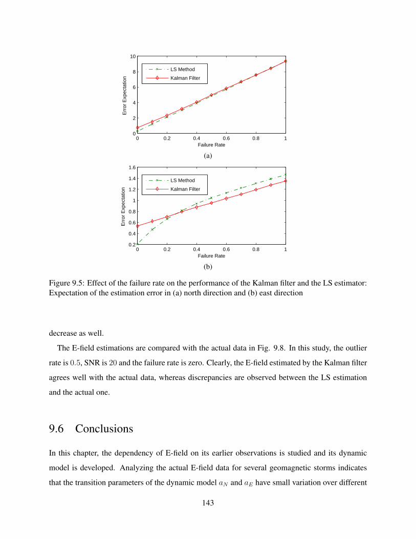
0 0.2 0.4 0.6 0.8 10
2
4
6
8
10
Failure Rate
Err
or E
xpec
tatio
n
LS Method
Kalman Filter
(a)
0 0.2 0.4 0.6 0.8 10.2
0.4
0.6
0.8
1
1.2
1.4
1.6
Failure Rate
Err
or E
xpec
tatio
n
LS Method
Kalman Filter
(b)
Figure 9.5: Effect of the failure rate on the performance of the Kalman filter and the LS estimator:Expectation of the estimation error in (a) north direction and (b) east direction
decrease as well.
The E-field estimations are compared with the actual data in Fig. 9.8. In this study, the outlier
rate is 0.5, SNR is 20 and the failure rate is zero. Clearly, the E-field estimated by the Kalman filter
agrees well with the actual data, whereas discrepancies are observed between the LS estimation
and the actual one.
9.6 Conclusions
In this chapter, the dependency of E-field on its earlier observations is studied and its dynamic
model is developed. Analyzing the actual E-field data for several geomagnetic storms indicates
that the transition parameters of the dynamic model aN and aE have small variation over different
143

0 0.2 0.4 0.6 0.8 10
0.5
1
1.5
Failure Rate
Err
or E
xpec
tatio
n
LS Method
Kalman Filter
(a)
0 0.2 0.4 0.6 0.8 10
0.2
0.4
0.6
0.8
Failure Rate
Err
or E
xpec
tatio
n
LS Method
Kalman Filter
(b)
Figure 9.6: Effect of the failure rate on the estimation error using the E-field data of a normal day:Expectation of the estimation error in (a) north direction and (b) east direction.
datasets. This enables development of a general dynamic model which approximates the dynamics
of any unknown E-field. Moreover, studying the E-field data of both stormy days and normal days,
it is observed that the dynamic model is less accurate for stormy days compared to normal days.
This chapter utilizes the system dynamics to improve the E-field estimation. The dynamic model
is integrated into the Kalman filter and better E-field estimation is obtained. The simulation results
indicate that the Kalman filter outperforms the LS estimator at higher Gaussian noise levels, higher
failure rates and higher outlier rates.
144

Figure 9.7: Effect of the E-field standard deviation on the accuracy of the Kalman filter.
18 19 20 21 22 23 24
−15
−10
−5
0
5
10
Time (hour)
E−
field
(m
V/k
m)
Actual E−Field
Kalman Filter
LS Method
Figure 9.8: Accuracy comparison of the Kalman filter and LS method.
145

CHAPTER 10
ENHANCED E-FIELD ESTIMATION UNDERMEASUREMENT UNCERTAINTIES
10.1 Introduction
This chapter investigates the uncertainties in the GIC measurements and evaluates their impacts
on the E-field estimation. Realistic noise scenarios for GIC measurements are considered and
various estimators are introduced to handle different type of uncertainties. The LS estimator is
used for GIC readings with white Gaussian noise, and the lease absolute value (LAV) estimator
is utilized to handle outliers. Ridge Regression (RR) estimator is proposed as an alternative to
LS method when additional information on the prior electric field is known. Moreover, a general
probabilistic GIC measurement model has been developed. Using the probabilistic model, the
accuracy and reliability of the LS estimator are derived analytically. The analytical results are
verified numerically using the WECC 9-bus system and the 20-bus test case. Similar to Chapter
9, this chapter contributes to the resiliency of power systems against GMDs by providing better
E-field estimation.
The chapter is organized as follows. LS, RR and LAV estimations are presented Section 10.2. In
Section 10.3, a probabilistic model for the GIC measurements is developed. The reliability analysis
of the LS estimator is the subject of Section 10.4. Numerical results are provided in Section 10.5.2
and the chapter is wrapped up in Section 10.6.
146
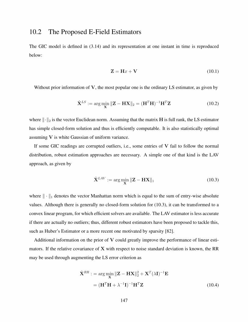
10.2 The Proposed E-Field Estimators
The GIC model is defined in (3.14) and its representation at one instant in time is reproduced
below:
Z = Hx+ V (10.1)
Without prior information of V, the most popular one is the ordinary LS estimator, as given by
XLS := arg minX‖Z−HX‖2 = (HTH)−1HTZ (10.2)
where ‖·‖2 is the vector Euclidean norm. Assuming that the matrix H is full rank, the LS estimator
has simple closed-form solution and thus is efficiently computable. It is also statistically optimal
assuming V is white Gaussian of uniform variance.
If some GIC readings are corrupted outliers, i.e., some entries of V fail to follow the normal
distribution, robust estimation approaches are necessary. A simple one of that kind is the LAV
approach, as given by
XLAV := arg minX‖Z−HX‖1 (10.3)
where ‖ · ‖1 denotes the vector Manhattan norm which is equal to the sum of entry-wise absolute
values. Although there is generally no closed-form solution for (10.3), it can be transformed to a
convex linear program, for which efficient solvers are available. The LAV estimator is less accurate
if there are actually no outliers; thus, different robust estimators have been proposed to tackle this,
such as Huber’s Estimator or a more recent one motivated by sparsity [82].
Additional information on the prior of V could greatly improve the performance of linear esti-
mators. If the relative covariance of X with respect to noise standard deviation is known, the RR
may be used through augmenting the LS error criterion as
XRR : = arg minX‖Z−HX‖22 + XT (λI)−1E
= (HTH + λ−1I)−1HTZ (10.4)
147

where λI is the relative covariance of X. By incorporating the prior information on X, the RR
is especially powerful in improving the numerical stability when H is ill-conditioned. However,
this introduces some bias on the estimator, which may be difficult to account for in practice. Note
that the three estimators either have closed form expression or can be solved as a linear program.
Hence, all the estimators enjoy low computational complexity.
10.3 Probabilistic Noise Modeling
Let z, x and v be the random variables representing the GIC measurements Z, the E-field X, and
the measurement noise V, respectively. Earlier investigations introduced white Gaussian noise,
nonuniform Gaussian noise and sensor failure as the three major sources of error in the GIC mea-
surements [54]. A general probabilistic model which captures these three types of measurement
error is presented in this section.
10.3.1 Additive White Gaussian Noise
The noise generated by many natural sources is in the form of white Gaussian noise. White Gaus-
sian noise is represented by a series of independent and identically distributed random variables
with normal distribution given by
v = Nn = N (0, σ2)m×1 (10.5)
where σ is the standard deviation of white Gaussian noise and m is the number of measurements.
10.3.2 Nonuniform Gaussian Noise
The Gaussian noise which is added to the GICs may not be identical for all the sensors and some
of the sensors may encounter higher noise levels. Corrupted outliers are subjected to Gaussian
noise with significantly higher standard deviation as given by
v = [N (0, σ2),N (0, s0σ2), · · · ,N (0, σ2)]T (10.6)
148

where so is the ratio of the noise level of the outliers to the normal measurements. This ratio is
assumed to be the same for all the outliers in the system. However, this is not a critical assumption
and more general models considering distinct outlier ratios can be developed.
A discrete random variable is defined to specify whether a sensor is an outlier as given by
uko :=
1, if the k-th sensor is outlier
0, if the k-th sensor is not outlier(10.7)
where uko is the outlier variable for the k-th sensor. The probability distribution of this random
variable is given by
Puo(i) :=
po, i = 1
1− po, i = 0(10.8)
where po is the outlier rate which is the probability of being an outlier and is assumed to be the
same for all the sensors.
10.3.3 Faulty Sensors
Sometimes, the GIC device fails to measure the GIC and the output of the sensor is a random
variable within the range of the sensor’s reading as given by
z = U(0, zmax) (10.9)
where U( , ) represents a random variable with uniform distribution and zmax is the maximum value
that the sensor can read.
A discrete random variable is defined to specify whether a sensor is faulty or not as given by
ukf :=
1, if the k-th sensor is faulty
0, if the k-th sensor is not faulty(10.10)
where ukf is the fault variable for the k-th sensor. The probability distribution of this random
149

variable is given by
Puf (i) :=
pf , i = 1
1− pf , i = 0(10.11)
In this equation, pf is the probability of being faulty and is assumed to be the same for all the
sensors. Nu = U(0, zmax)m×1 is a vector of random variables with uniform distributions and is
defined to represent the output of the faulty sensors.
10.3.4 Probabilistic Measurement Model
Using the random variables defined earlier, one can develop a general measurement model which
captures various noise scenarios as given by
z =(1− uf ) · (Hx+ ([1]m×1 + (so − 1)uo) ·Nn)
+uf ·Nu (10.12)
Note that in this model, uf and Nu are used to characterize the faulty sensors, uo captures the
outliers and Nn accounts for the uniform Gaussian noise scenario. The proposed measurement
model is useful for studying the probability distribution of the estimation error and consequently
evaluating the reliability of the estimator.
10.4 Reliability Analysis
The reliability of a system is the probability that it performs its intended function without failure
for a specific period of time. The reliability of a system decays exponentially over time when the
failure rate of the system is constant.
The reliability of an estimator is defined as the probability that its error does not exceed a thresh-
old for a specific period of time. To calculate the estimator reliability, the probability distribution
of the estimation error is studied and the estimator failure rate is calculated accordingly. Assuming
150

Figure 10.1: Probability distribution of the estimation error and the estimator failure rate.
constant failure rate for the estimator over time, the reliability of the estimator is determined by
R(t) = Prt < Tf = e−λt (10.13)
where λ is the failure rate of the estimator and Tf is the estimator time to failure.
To obtain the estimator failure rate, the probability distribution of the estimation error is re-
quired. The probability of estimation error has normal distribution when the observation noise
is Gaussian. Hence, calculating the first and second moments of the estimation error completely
parameterizes the error distribution. The probability distribution of the estimation error and the
estimator failure rate under the Gaussian noise scenario are shown in Fig. 10.1.
Note that when there are faulty sensors in the system, the measurement noise is no longer Gaus-
sian. In this case, the probability of the error no longer follows a normal distribution, and fitting
it with a normal distribution causes inaccuracy in the reliability assessment. This phenomenon is
demonstrated through an example in Section 10.5.2.
10.4.1 Expectation of Estimation Error
The probabilistic model in (10.12) is used to derive the expectation of GIC measurement as given
by
E[z] = (1− pf )HE[x] + pfzmax
2× [1]m×1 (10.14)
151

The estimated state obtained by LS estimation is presented in (10.2). Deriving the expectation
of the estimated state from (10.2) and substituting into (10.14) gives rise to
E[x] = (1− pf )E[x] + pfZmax
2(HTH)−1HT [1]N×1 (10.15)
The expectation of electric field is zero, which zeros out the first term in (10.15). In the GIC
model, the sum of entry-wise values of the columns in matrix H is zero, which zeros the second
term in (10.15) as well. Hence, the expectation of estimation error is zero as given by
E[e] = E[x− x] = E[x]− E[x] = 0 (10.16)
10.4.2 Second Moment of Estimation Error
To compute the second moment of the estimated state, the second moment of the observation
should be determined as proposed by
xxT = (HTH)−1HT zzT (HTH)−1HT (10.17)
Using the GIC probabilistic model, the second moment of the observation is computed by
E[zzT ] = (E[(1− uf )(1− uf )T ]) · (HE[xxT ]HT )
+(s0 − 1)2E[(1− uf )(1− uf )T ] · E[uouTo ] · E[NnN
Tn ] + E[NuN
Tu ] · E[ufu
Tf ] (10.18)
where the cross moments of Nu, uo and Nn are given by
E[NuNTu ](ij) =
z2max3, i = j
z2max4, i 6= j
E[uouTo ](ij) =
po, i = j
p2o, i 6= j
E[NnNTn ](ij) =
σ2, i = j
0, i 6= j(10.19)
152

To compute E[zzT ], E[xxT ] which is the second moment of the actual state should be de-
termined as proposed by (10.18). If prior information on the variance of the actual state is not
available, a realistic state model should be developed to estimate it. A basic generative model for
the electric field is x = [cos(θ) sin(θ)]T where θ = U(0, 2π) is the angle of electric filed. Using
more realistic models for the electric field provides higher accuracy. Future studies can extend this
work by including more realistic models.
The power series for cos2θ, sin2θ and cosθsinθ at θ = 0 are given bysin2θ =
∞∑k=1
(−1)k−122k−1x2k
(2k!)
sinθcosθ =∞∑k=0
(−1)k22kx2k+1
(2k+1!)
cos2θ = 1− sin2θ
(10.20)
These power series are used for calculating the second moment of the state as given by
E[xxT ] =
E[cos2θ] E[sinθcosθ]
E[sinθcosθ] E[sin2θ]
=
0.5 0
0 0.5
(10.21)
The second moment of estimation error is calculated by
E[eeT ] = E[xxT ]− (2pf − 1)
0.5 0
0 0.5
(10.22)
10.5 Numerical Results
In this section, the accuracy of the LS, LAV and RR estimators under various noise scenarios is
evaluated through numerical results. Moreover, analytical and numerical results are presented for
the reliability analysis of the LS estimator.
153

G
G
G
Sub 1
Sub 2 Sub 3
Sub 4 Sub 5
Sub 6
T1
T2
T3
13.8 KV
230 KV
Figure 10.2: Single-line diagram of the 9-bus test case.
Table 10.1: Substation Location and Grounding Resistance for the 9-bus Test Case
Name Latitude Longitude Grounding Resistance (Ω)Sub1 39 -88 0.38Sub2 41 -89 0.38Sub3 40 -87 0.38Sub4 40 -88.5 0.47Sub5 40.5 -88 0.47Sub6 39.5 -87.5 0.47
10.5.1 Estimators Accuracy Evaluation
The first test case to study is a 9-bus system which is modified from the WECC standard 9-bus
system [55] by including bus geographic coordinates, transformer neutral resistances, etc. This
test case has six substations and three transformers as illustrated in Fig. 10.2. The geographic
locations of the substations and their grounding resistances are presented in Table 10.1.
Variable electric field is enforced to the system. The magnitude of the enforced electric field is
one and its angle is a random variable between 0 and 2π with uniform distribution. Monte Carlo
simulation with 1000 realizations is investigated to perfectly simulate the randomness of electric
field angle.
154

4 6 8 10 12 14 160
0.5
1
1.5
SNR
Err
or
LAV EstimatorRR EstimatorLS Estimator
(a)
4 6 8 10 12 14 160
0.2
0.4
0.6
0.8
1
SNR
Err
or
LAV EstimatorRR EstimatorLS Estimator
(b)
Figure 10.3: Estimation error versus SNR for the 9-bus test case under uniform Gaussian noise:(a) magnitude and (b) angle of electric field.
Table 10.2: Transformers Coefficients for the 9-bus Test Case
Name HN HE
T1 -35.638 1.999T2 49.358 -46.47T3 -13.721 44.471
The GICs induced by the electric field are determined via solving the GIC flow program in Pow-
erWorld Simulator. Table 10.2 presents the coefficients of the three transformers. The coefficient
matrix is full rank which ensures the effectiveness of LS estimator.
The GICs obtained from the GIC flow program represent ideal measurements. The noisy mea-
surements are obtained by adding white Gaussian or nonuniform noise to the ideal GIC values.
The investigated Monte Carlo simulation incorporates the randomness in additive noise. Figure
155

4 6 8 10 12 14 160
1
2
3
4
SNR
Err
or
LAV EstimatorRR EstimatorLS Estimator
(a)
4 6 8 10 12 14 160.2
0.4
0.6
0.8
1
1.2
SNR
Err
or
LAV EstimatorRR EstimatorLS Estimator
(b)
Figure 10.4: Estimation error versus SNR for the 9-bus test case under nonuniform Gaussian noise:(a) Magnitude and (b) angle of Electric Field.
10.3 illustrates the accuracy of LS, RR, and LAV estimators when the GIC measurements are sub-
jected to white Gaussian noise. Clearly, the LS estimator outperforms the LAV in estimating both
magnitude and angle when the measurement noise is purely white Gaussian.
Ridge Regression (RR) estimator can be used as an alternative to LS estimator when the relative
covariance of the electric field is known. The additional information on V improves the perfor-
mance as illustrated in Fig. 10.3. The advantage of the RR estimator over the LS is more for
smaller SNRs which encourages the application of the former at higher noise levels. Moreover,
the improvement of the RR estimator over the LS estimator is higher for the magnitude than for
the angle.
To have nonuniform noise, the noise standard deviation at the third substation is increased by 5
times, which means the corresponding measurement can be considered as an outlier. Figure 10.4
156

shows the improvement of LAV estimator over the LS under this setup. Comparing the uniform
and nonuniform noise scenarios, the LAV estimation error is almost the same for both uniform
and nonuniform noise scenarios, whereas the LS estimation error is significantly higher for the
nonuniform noise scenario.
Employing RR estimator instead of the LS improves the estimations in the same fashion as the
uniform noise scenario. In fact, the accuracy of RR estimator in magnitude estimation is as good
as that of the LAV under this setup, which results from the additional information.
Next, the accuracy of the three estimators is evaluated in the case of faulty sensors. To simulate
this, the GIC at the third substation is replaced by a white Gaussian noise which has zero coherence
with the original GIC. The standard deviation of the replaced Gaussian noise is equal to the GIC
norm at the substation. The accuracy of the LS and RR estimators decreases significantly in the
presence of faulty sensors as shown in Fig. 10.5. The accuracy of the LAV estimator is not affected
as it detects the outliers and eliminates them from the estimations process.
The second test case to study is the 20-bus system. Similar to the 9-bus test case, an E-field
is enforced to the system which has unity magnitude and random angle with uniform distribution
between 0 and 2π. Figure 10.6 illustrates the error norm for all three estimators when the GIC
measurements are subjected to white Gaussian noise. Clearly, LS and RR estimators outperform
the LAV under this setup. To generate nonuniform noise, one of the transformers is randomly
selected and the standard deviation of its noise is increased by 5 times. The randomness of this se-
lection is modeled through Monte Carlo simulation. The accuracy of the LAV estimator improves
over the LS and RR under this noise scenario as shown in Fig. 10.7.
The accuracy comparison of the RR and LS estimators for the 20-bus system agrees with that
for the 9-bus test case. For both systems, the improvement of the RR estimator is higher for the
magnitude estimation and also at smaller SNRs. Comparing the results for the two test cases, one
can conclude that the advantage of the RR estimator over the LS is more for the smaller systems.
This may relate to the data redundancy in the larger system which reduces the advantage of prior
knowledge about X.
In Fig. 10.8, the number of outliers is increased by randomly selecting more transformers and
increasing their noise level by five times. Clearly, the number of outliers does not limit the perfor-
mance of the LAV estimator and this estimator outperforms the others for any number of outliers.
157

4 6 8 10 12 14 160
0.5
1
1.5
2
2.5
SNR
Err
or
LAV EstimatorRR EstimatorLS Estimator
(a)
4 6 8 10 12 14 160.2
0.4
0.6
0.8
1
1.2
1.4
SNR
Err
or
LAV EstimatorRR EstimatorLS Estimator
(b)
Figure 10.5: Estimation error versus SNR for the 9-bus system and in the case of having faultysensors: (a) Magnitude and (b) angle of Electric Field.
To investigate faulty measurements, one of the transformers is randomly selected and its GIC is
replaced by white Gaussian noise. The standard deviation of the replaced Gaussian noise is equal
to the Manhattan norm of the transformer GIC. The accuracy comparison of the three transformers
under this setup is illustrated in Fig. 10.9. Similar to the 9-bus system, LAV estimator outperforms
the other two for this noise scenario.
10.5.2 Reliability Analysis of the LS Estimator
In this section, the analytical derivations of the error distribution and the reliability for the LS
estimator are verified through numerical results. Variable electric field is enforced to the system.
The magnitude of the enforced electric field is 1( Vkm
) and its angle is a random variable between 0
158

4 6 8 10 12 14 160
0.1
0.2
0.3
0.4
0.5
SNR
Err
or
LAV EstimatorRR EstimatorLS Estimator
(a)
4 6 8 10 12 14 160
0.1
0.2
0.3
0.4
SNR
Err
or
LAV EstimatorRR EstimatorLS Estimator
(b)
Figure 10.6: Estimation error versus SNR for the 20-bus test case under uniform Gaussian noise:(a) Magnitude and (b) angle of Electric Field.
and 2π with uniform distribution. Monte Carlo simulation with 1000 realizations is investigated to
simulate the angle randomness.
The GICs induced by the electric field are determined via solving the GIC flow program in Pow-
erWorld Simulator. The GICs obtained from the GIC flow program represent ideal measurements.
The probabilistic model in (10.12) is used to obtain the noisy measurements and Monte Carlo sim-
ulation is used to simulate its randomness. The analytical results presented earlier indicate that
the expectation of estimation error is zero. Monte Carlo simulation is used to calculate the error
expectation in the north direction and a similar result is obtained as shown in Fig. 10.10. For
conciseness, the results are presented only in the north direction throughout the subsection.
The second moment of the estimation error direction at different failure rates is illustrated in
Fig. 10.11. The Gaussian noise level and outlier rate are set to zero in this study. Clearly, the
159
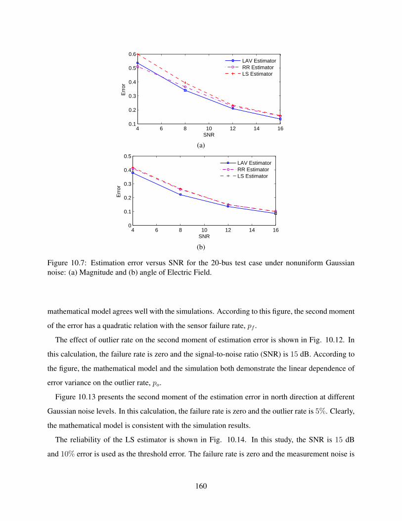
4 6 8 10 12 14 160.1
0.2
0.3
0.4
0.5
0.6
SNR
Err
or
LAV EstimatorRR EstimatorLS Estimator
(a)
4 6 8 10 12 14 160
0.1
0.2
0.3
0.4
0.5
SNR
Err
or
LAV EstimatorRR EstimatorLS Estimator
(b)
Figure 10.7: Estimation error versus SNR for the 20-bus test case under nonuniform Gaussiannoise: (a) Magnitude and (b) angle of Electric Field.
mathematical model agrees well with the simulations. According to this figure, the second moment
of the error has a quadratic relation with the sensor failure rate, pf .
The effect of outlier rate on the second moment of estimation error is shown in Fig. 10.12. In
this calculation, the failure rate is zero and the signal-to-noise ratio (SNR) is 15 dB. According to
the figure, the mathematical model and the simulation both demonstrate the linear dependence of
error variance on the outlier rate, po.
Figure 10.13 presents the second moment of the estimation error in north direction at different
Gaussian noise levels. In this calculation, the failure rate is zero and the outlier rate is 5%. Clearly,
the mathematical model is consistent with the simulation results.
The reliability of the LS estimator is shown in Fig. 10.14. In this study, the SNR is 15 dB
and 10% error is used as the threshold error. The failure rate is zero and the measurement noise is
160
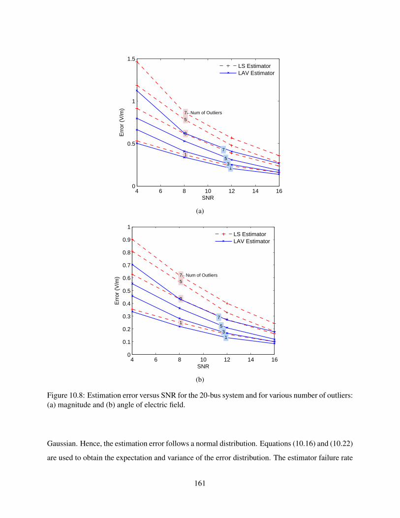
4 6 8 10 12 14 160
0.5
1
1.5
1
1
3
3
5
5
7
7
←Num of Outliers
SNR
Err
or (
V/m
)
LS EstimatorLAV Estimator
(a)
4 6 8 10 12 14 160
0.1
0.2
0.3
0.4
0.5
0.6
0.7
0.8
0.9
1
1
1
3
3
5
5
7
7
←Num of Outliers
SNR
Err
or (
V/m
)
LS EstimatorLAV Estimator
(b)
Figure 10.8: Estimation error versus SNR for the 20-bus system and for various number of outliers:(a) magnitude and (b) angle of electric field.
Gaussian. Hence, the estimation error follows a normal distribution. Equations (10.16) and (10.22)
are used to obtain the expectation and variance of the error distribution. The estimator failure rate
161

4 6 8 10 12 14 160
0.5
1
1.5
SNR
Err
or (
V/m
)
LAV EstimatorRR EstimatorLS Estimator
(a)
4 6 8 10 12 14 160
0.2
0.4
0.6
0.8
SNR
Err
or (
V/m
)
LAV EstimatorRR EstimatorLS Estimator
(b)
Figure 10.9: Estimation error versus SNR for the 20-bus system and in the case of having faultysensors: (a) magnitude and (b) angle of electric field.
0 5 10 15 20−0.01
−0.005
0
0.005
0.01
SNR
Err
or E
xpec
tatio
n (p
u)
Simulation
Mathematical Model
Figure 10.10: Expectation of estimation error at different Gaussian noise levels.
162

0 0.2 0.4 0.6 0.8 10
0.5
1
1.5
Failure Rate
Sec
ond
Mom
ent o
f Err
or (
pu)
Simulation
Mathematical Model
Figure 10.11: Effect of failure rate on the second moment of LS estimation error.
0 0.2 0.4 0.6 0.8 10
0.02
0.04
0.06
0.08
0.1
0.12
0.14
0.16
0.18
Outlier Rate
Sec
ond
Mom
ent o
f Err
or (
pu)
Simulation
Mathematical Model
Figure 10.12: Effect of outlier rate on the second moment of LS estimation error.
is calculated according to Fig. 10.1 and the reliability is determined accordingly. In the figure,
the analytical model and the simulation are termed as “AM” and “Sim”, respectively. Clearly, the
analytical model agrees well with the simulation.
According to Fig. 10.14, the reliability curves follow exponential decay and their time constants
depend on the sensor outlier rate. The variation of estimator failure rate with the sensor outlier rate
is shown in Fig. 10.15. The reliability of the estimator declines as the outlier rate increases.
163

0 5 10 15 20 250
0.05
0.1
0.15
0.2
0.25
0.3
0.35
SNR
Sec
ond
Mom
ent o
f Err
or (
pu)
Simulation
Mathematical Model
Figure 10.13: Second moment of LS estimation error and its variation with Gaussian noise level.
0 5 10 15 20 25 300
0.2
0.4
0.6
0.8
1
Time Step
Rel
iabi
lity
Sim, po=0.02
AM, po=0.02
Sim, po=0.05
AM, po=0.05
Sim, po=0.2
AM, po=0.2
Figure 10.14: Reliability of LS estimator at different outlier rates.
Figure 10.16 illustrates the effect of Gaussian noise level on the estimator failure rate. In this
calculation, the failure rate is zero and the outlier rate is 5%. The mathematical model provides
good accuracy in calculating the estimator failure rate.
Variation of the estimator failure rate with the sensor failure rate is presented in Fig. 10.17.
The Gaussian noise level and outlier rate are set to zero. When the sensor failure rate is not
zero, the measurement noise is not Gaussian and the assumption of having normally distributed
164

0 0.05 0.1 0.15 0.20
0.1
0.2
0.3
0.4
0.5
0.6
0.7
Sensors Outlier Rate
Est
imat
or F
ailu
re R
ate
Simulation
Mathematical Model
Figure 10.15: Variation of estimator failure rate with the outlier rate of the sensor.
16 17 18 19 20 21 22 23 24 250
0.05
0.1
0.15
0.2
0.25
SNR
Est
imat
or F
ailu
re R
ate
Simulation
Mathematical Model
Figure 10.16: Effect of Gaussian noise level on the estimator failure rate.
0 0.05 0.1 0.15 0.20
0.5
1
1.5
Sensors Failure Rate
Est
imat
or F
ailu
re R
ate
Simulation
Mathematical Model
Figure 10.17: Variation of the estimator failure rate with the failure rate of the sensors.
165

error no longer holds. Hence, the mathematical model fails to accurately estimate the reliability
and a discrepancy is observed between the mathematical model and the simulation. A possible
approach to solve this problem is to calculate the higher order moments of the estimation error and
approximate the error distribution based on its higher order moments. Further studies are necessary
to tackle this problem.
10.6 Conclusions
This chapter analyzes the impact of the GIC measurement error on the accuracy of the E-field es-
timation. Realistic noise scenarios are considered for GIC measurements and suitable estimators
are proposed to handle different types of uncertainties. A probabilistic model for GIC measure-
ments has been developed. Using the developed model, the moments of the estimation error are
calculated. Moreover, an analytical model for assessing the estimator’s reliability has been devel-
oped. Numerical results indicate that the proposed model can effectively evaluate the estimator’s
reliability when the system is subject to Gaussian noise. In the case of faulty sensors, the estima-
tion error no longer follows the normal distribution and thus the proposed reliability assessment
technique fails. This opens up future research on enhancing the reliability assessment framework
with respect to sensor failures.
166

CHAPTER 11
ADDING GMD MODELS TO THE EXISTING TESTCASES
11.1 Introduction
Realistic public test cases can facilitate the studies on the GMDs impacts on the power system by
providing a benchmark to validate the related analysis tools. Many standard test cases are available
for different aspects of power system analysis. These cases are designed for ac analysis and do not
contain the necessary inputs such as the substation grounding resistances and the geographic coor-
dinates which are essential for GMD studies. In this chapter, a framework is proposed to generate
GMD-related parameters for the existing standard power system test cases. The substation geo-
graphic coordinates are the key parameters which are missing in the existing cases. The Kamada
and Kawai (KK) algorithm and the Force-directed (FD) method are presented as two effective
graph drawing algorithms to generate the geographic layout and determine the coordinates. The
effectiveness of the proposed framework is evaluated through numerical results using the 20-bus
system and the IEEE 24-bus system.
The tool developed in this chapter can improve many aspects of the GMD analysis by providing
suitable benchmarks for evaluation purposes. This includes all the GMD-related studies in this
thesis. Most of the analysis is performed on the 20-bus system since it is one of the few test cases
available for GMD studies. Extending the analysis to other systems can provide better performance
evaluation.
The chapter is organized as follows: The framework for determining the GIC-related parameters
is presented in Section 11.2. Section 11.3 demonstrates the proposed technique through numerical
results. Section 11.4 presents a conclusion and direction for future work.
167

11.2 Determining the GIC-related Parameters
The key parameters required for GMD analysis, which are usually missing in standard test cases,
are the substation grounding resistances and geographic coordinates. A rather simplistic model for
determining the substation grounding resistances is used in [45]. In this model, the assumed resis-
tance depends on the highest substation voltage level and its assumed size (based on the number of
lines coming into the substation), with larger, higher voltage substations having lower values. Soil
resistivity, which certainly can have an impact, is not included in this simplistic model. Ballpark
values are usually substantially below 0.5Ω for 230kV and above substations, and between 1 and
2Ω for the lower voltage substations.
The geographic coordinates may be obtained through developing a geographic layout of the
system using the existing graph drawing techniques as described in the following.
11.2.1 Force-directed Graph Drawings
Force-directed graph drawings is a method for drawing graphs in a way that looks pleasant to the
eye [93]. The vertices of the graph are positioned in two-dimensional or three-dimensional space so
that the edges are about the same length and the number of crossings is minimized. The algorithm
assigns forces among the set of edges and the set of vertices and uses these forces to simulate
the movement of the vertices or to minimize their energy. Attractive forces like springs are used
to attract the vertices that are connected in the graph (based on Hooke’s law). Repulsive forces
like electrically charged particles are used to separate all pairs of vertices (based on Coulomb’s
law). The layout is obtained by solving for the equilibrium state of this system of forces. In
equilibrium, the edges have similar lengths because of the spring attractions and the vertices are as
far as possible from each other due to the electric repulsive forces.
The attractive and repulsive forces between a pair of vertices are defined as fa(d) = d2
k
fr(d) = −k2
d
(11.1)
where fa and fr are respectively the attractive and repulsive forces and d is the distance between
168

the pair of vertices. k is the optimal distance between the vertices as given by
k = C
√area
number of vertices(11.2)
where C is a constant.
11.2.2 Kamada and Kawai Algorithm
the FD method does not preserve the distances between the vertices and the edges and the resulting
layout has uniform lengths. Sometimes, it is desired to maintain the distances, especially in GMD
applications where the line lengths have significant impact on the GIC flows. the KK algorithm
minimizes the difference between the ideal lengths and actual ones instead of minimizing the num-
ber of edge crossings [94]. Unlike the FD algorithm, no repulsive forces are considered between
vertices. Spring forces are used between all pairs of vertices, with ideal spring lengths equal to the
vertices’ graph-theoretic distance. The optimal layout is obtained by minimizing the total spring
energy.
Let n be the number of vertices and p1, p2, · · · , pn be the particles in a plane representing the
vertices v1, v2, · · · , vn respectively. The energy of the system is given by
E =n−1∑i=1
n∑j=i+1
1
2kij(|pi − pj| − lij) (11.3)
where lij is the desired length of the spring between pi and pj and is calculated by
lij =L0
maxi≤j
dijdij (11.4)
where dij is the distance between vi and vj and L0 is the length of the display area. kij is the
strength of the spring between pi and pj as expressed in:
kij =Kspr
d2ij(11.5)
where Kspr is a constant. For a two-dimensional space, the particle pi is represented by the rect-
169

angular coordinates (xi, yi) and the system energy in (11.3) is given by
E =n−1∑i=1
n∑j=i+1
1
2kij(xi − xj)2 + (yi − yj)2
+ l2ij − 2lij
√(xi − xj)2 + (yi − yj)2 (11.6)
The necessary condition of the local minimum is as follows:
∂E
∂xm=
∂E
∂ym= 0, 1 ≤ m ≤ n (11.7)
The partial derivative of the energy with respect to x and y is expressed in:
∂E
∂xm=∑i 6m
kmi(xm − xi)−lmi(xm − xi)√
(xm − xi)2 + (ym − yi)2
∂E
∂ym=∑i 6m
kmi(ym − yi)−lmi(xm − xi)√
(xm − xi)2 + (ym − yi)2 (11.8)
This gives rise to a system of 2n nonlinear equations and Newton-Raphson may be used for solving
it.
Note that KK requires the line lengths as input. However, the lengths are not usually available
for the synthetic cases. To address this, the line resistances may be used as a criterion to determine
the lengths. The line resistance depends on its conductor type, the conductor bundling structure and
the length. The conductor type and the bundling structure depend on the voltage level. Heuristics
may be developed to get the resistance per meter for different voltage levels through the statistical
analysis of the real power systems. Using the resistance (available in standard test cases) and the
estimated resistance per line, the line length can be estimated.
11.3 Numerical Results
In this section, the geographic layouts of two power systems are developed using the proposed
algorithms. The first system to study is the 20-bus system in [38]. This test case includes many
features found in typical high voltage transmission networks. The case is designed specifically
170

32.5 33 33.5 34 34.5−88
−87
−86
−85
−84
−83
−82
−81
−80
1
2
3
4
5
6 7
8
Latitude
Long
itude
Figure 11.1: Geographic layout of the system using the available coordinates.
for GMD applications and contains substation geographic coordinates. Figure 11.1 illustrates the
geographic layout of the system using the available coordinates.
The KK algorithm is utilized to develop a geographic layout. The coordinates are not provided to
the algorithm and are to be estimated. Instead, the line lengths are calculated from the coordinates
and are given to the algorithm:
a = sin2(φ2 − φ1
2) + cos(φ1)cos(φ2)sin
2(λ2 − λ1
2)
c = 2atan2(√a,√
1− a)
d = Rc (11.9)
where φ and λ are latitude and longitude respectively, d is the distance between points 1 and 2 (in
mile), and R is the Earth radius, i.e. 6,371 km. Figure 11.2 illustrates the resulting layout obtained
from KK algorithm. Comparing this layout with the actual one in Fig. 11.1, it is observed that
the layout developed by the KK algorithm preserves the lengths, but does not capture the original
layout. This is because developing the layout from only the line lengths does not provide a unique
solution and additional information is required to retrieve the original layout.
The line lengths are calculated for the layout developed by the KK algorithm and are compared
171
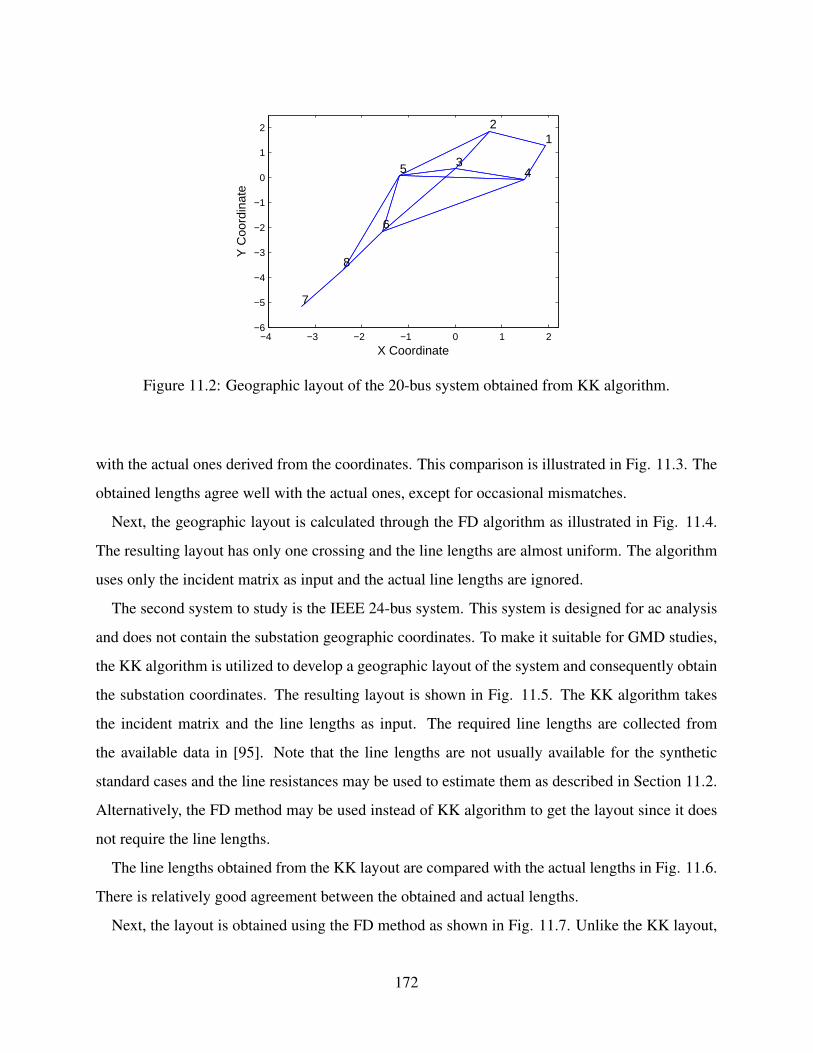
−4 −3 −2 −1 0 1 2−6
−5
−4
−3
−2
−1
0
1
21
2
345
6
7
8
X Coordinate
Y C
oord
inat
e
Figure 11.2: Geographic layout of the 20-bus system obtained from KK algorithm.
with the actual ones derived from the coordinates. This comparison is illustrated in Fig. 11.3. The
obtained lengths agree well with the actual ones, except for occasional mismatches.
Next, the geographic layout is calculated through the FD algorithm as illustrated in Fig. 11.4.
The resulting layout has only one crossing and the line lengths are almost uniform. The algorithm
uses only the incident matrix as input and the actual line lengths are ignored.
The second system to study is the IEEE 24-bus system. This system is designed for ac analysis
and does not contain the substation geographic coordinates. To make it suitable for GMD studies,
the KK algorithm is utilized to develop a geographic layout of the system and consequently obtain
the substation coordinates. The resulting layout is shown in Fig. 11.5. The KK algorithm takes
the incident matrix and the line lengths as input. The required line lengths are collected from
the available data in [95]. Note that the line lengths are not usually available for the synthetic
standard cases and the line resistances may be used to estimate them as described in Section 11.2.
Alternatively, the FD method may be used instead of KK algorithm to get the layout since it does
not require the line lengths.
The line lengths obtained from the KK layout are compared with the actual lengths in Fig. 11.6.
There is relatively good agreement between the obtained and actual lengths.
Next, the layout is obtained using the FD method as shown in Fig. 11.7. Unlike the KK layout,
172
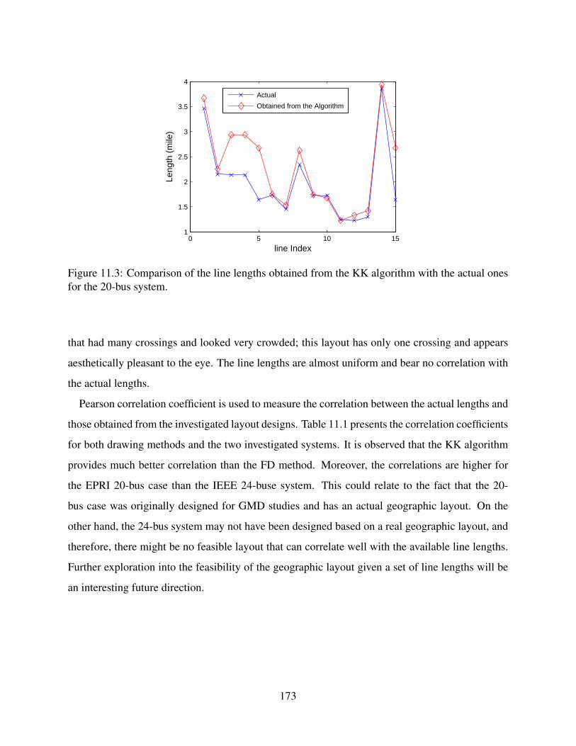
0 5 10 151
1.5
2
2.5
3
3.5
4
line Index
Leng
th (
mile
)
Actual
Obtained from the Algorithm
Figure 11.3: Comparison of the line lengths obtained from the KK algorithm with the actual onesfor the 20-bus system.
that had many crossings and looked very crowded; this layout has only one crossing and appears
aesthetically pleasant to the eye. The line lengths are almost uniform and bear no correlation with
the actual lengths.
Pearson correlation coefficient is used to measure the correlation between the actual lengths and
those obtained from the investigated layout designs. Table 11.1 presents the correlation coefficients
for both drawing methods and the two investigated systems. It is observed that the KK algorithm
provides much better correlation than the FD method. Moreover, the correlations are higher for
the EPRI 20-bus case than the IEEE 24-buse system. This could relate to the fact that the 20-
bus case was originally designed for GMD studies and has an actual geographic layout. On the
other hand, the 24-bus system may not have been designed based on a real geographic layout, and
therefore, there might be no feasible layout that can correlate well with the available line lengths.
Further exploration into the feasibility of the geographic layout given a set of line lengths will be
an interesting future direction.
173

−4 −3 −2 −1 0 1 2 3
−4
−3
−2
−1
0
1
2
3
4
1
2
34
56
7
8
X Coordinate
Y C
oord
inat
e
Figure 11.4: Geographic layout of the 20-bus system obtained from FD method.
Table 11.1: Grounding Resistances of the 20-bus Test Case
Test Case Kamada-Kawai Force-directedIEEE 24-bus 0.694 0.1711EPRI 20-bus 0.8554 0.3441
11.4 Conclusions
In this chapter, a framework is proposed to incorporate GMD modeling into the already existing
standard power system cases. The geographic coordinates are the key parameters that are missing
in the standard cases and are essential for GMD studies. KK and BF are presented as two effective
graph drawing techniques to generate the geographic layout and consequently get the coordinates.
The proposed framework is applied to the 20-bus and 24-bus systems and their coordinates are
determined. Numerical results indicate that the layout obtained from KK preserves the line lengths,
while BF provides a layout which is aesthetically pleasing, but its resulting lengths have little
correlation with the actual lengths.
The study suggests several directions for future research: First, the algorithm can be applied to
other standard test cases such as the IEEE 118-bus or 300-bus systems. Second, the algorithm for
estimating the line lengths from their resistances were described briefly. This algorithm can be fur-
174

−50 0 50 100−150
−100
−50
0
50
100
12
3
4
56
78
913
1415
161718
19
20
21
22
23
X Coordinate
Y C
oord
inat
e
Figure 11.5: Geographic layout of the IEEE 24-bus system obtained from KK algorithm.
ther refined and statistical analysis of the actual systems may be utilized to verify its effectiveness.
Last, the effectiveness of the test cases generated from the proposed framework may be validated
by performing GMD studies on the generated case and evaluating the results.
175

0 5 10 15 20 25 30 350
20
40
60
80
100
120
line Index
Leng
th (
mile
)
ActualObtained from Algorithm
Figure 11.6: Comparison of the line lengths obtained from the KK algorithm with the actual onesfor the 24-bus system.
−10 −5 0 5 10−10
−5
0
5
10
1 2
3 4
56
7
8
9
1314
15
1617
18
19 20
21
22
23
X Coordinate
Y C
oord
inat
e
Figure 11.7: Geographic layout of the IEEE 24-bus system obtained from FD method.
176

CHAPTER 12
CONCLUSION
In this chapter, a summary of the thesis is presented and the main contributions are highlighted.
The chapter concludes with final remarks and future research directions.
12.1 Summary and Contributions
Chapter 2. In this chapter, we develop two generation redispatch algorithms which improve the
power system resiliency against cyber attacks. ROPF modifies the conventional OPF with the ob-
jective of optimizing resiliency instead of the generation cost. Security-compliant control subspace
synthesis is a greedy algorithm that has lower computational complexity and is suitable for online
RAS applications. Numerical results on the small IEEE 24-bus test case indicate that both methods
provide sufficient security for the system with reasonable running time. For a larger case like the
IEEE 118-bus system, ROPF offers extremely good security, yet the running time is quite high for
online applications. On the other hand, the greedy algorithm offers a solution that is less secure,
but much faster to compute.
Chapter 3. This chapter provides some background on GMDs, their negative impacts and the
importance of their modeling. GIC modeling is presented in detail and methods to estimate the
E-field using both magnetic and GIC data are developed.
Chapter 4. In this chapter, a novel line switching algorithm is developed to mitigate the GMD neg-
ative impacts. The algorithm minimizes the GIC-saturated reactive power loss based on TLODFs
(counterparts of LODFs in GIC analysis). Some aspects of the AC analysis are considered to pro-
vide sufficient AC-related security measures. The computational complexity of the algorithm is
analyzed and heuristics are utilized to reduce its running time for large-system applications. The
177

algorithm performance is evaluated through numerical results using the small 20-bus system, the
medium-size UIUC 150-bus system and the large Texas 2000-bus case. The algorithm provides an
effective tool to minimize the transformer damage during GMDs and improve the resiliency.
Chapter 5. This chapter investigates how to validate the GIC model using a modeless, SVD-
based approach. Under an ideal uniform electric field, there exists a linear relation between the
transformer GIC values and the E-field. Nonetheless, without accurate information of the power
network topology and dc conductances, it becomes extremely difficult to characterize such linear
dependency and accordingly estimate the E-field for validation. To tackle this, further analysis of
the geomagnetic data suggests that the GIC matrix formed by different transformers across time
will have rank-2 and the right singular vectors can be used to infer the E-field. This SVD-based ap-
proach has validated the linear relation using a realistic test case. The validation framework is also
extended to account for non-uniform E-field and is successfully demonstrated through simulation.
GMD modeling is a fundamental part of the GMD mitigation and the validation tool presented in
this chapter can contribute to the resiliency against GMDs by improving the associated models.
The work presented in this chapter was published in [59].
Chapter 6. In this chapter, a novel validation technique is presented which utilizes the network
parameters (when available) to provide a stronger validation tool. This method introduces the
transformer scales to account for the system uncertainties and provides the extra capability of
detecting the outlier measurements. The proposed validation framework is demonstrated using a
PowerWorld case study and its performance is extensively studied under various scenarios. More
interesting real data validation is conducted using the GIC measurements provided by ATC. The
data from five transformers are validated and the existing outlier in the set of the measurements is
successfully detected. The work presented in this chapter was published in [60].
Chapter 7. In this chapter, an analytical technique is developed which derives the substation
grounding resistances from the GIC measurements. In this technique, the relation between the
GICs and the grounding resistances is linearized through some sensitivity parameters and linear
regression is used to solve for the resistances. The uncertainty in the grounding resistances in-
troduces error to the parameters of the linear model. To tackle this, the problem is reformulated
178
to decouple the uncertainties from the known parameters and regularized least squares is used for
solving it. The effectiveness of the algorithm is evaluated using both a small test case as well as
a 62,500 bus model of the EI system. As demonstrated, the algorithm can estimate the grounding
resistances accurately even when the available GIC measurements are sparse and the assumed re-
sistances have large error. The proposed technique reduces the uncertainties of the GMD model
by providing more accurate grounding resistances. This improves the resiliency to GMDs through
better assessment of the GICs and their risks. The work presented in this chapter was published in
[61].
Chapter 8. In this chapter, the magnetic field measurements at 21 observatories in North Amer-
ica over a three-year period are extensively studied and various statistical measures are extracted
from the data. Correlation analysis is performed to capture the possible dependencies between the
observatories. It is observed that the magnetic fields at some observatories are highly correlated
and this dependency is not always related to their geographic distance. To address this, the inverse
distance weighting interpolation is modified to account for such dependencies. The modified inter-
polation improves over the conventional one as demonstrated through real data analysis. Finally,
the correlation analysis is extended to the frequency domain using the wavelet transform. The pro-
posed technique contributes to the resiliency by providing a better assessment of the GMD risks at
distinct locations in the network. The work presented in this chapter was published in [62].
Chapter 9. In this chapter, the dependency of E-field on its earlier observations is studied and
its dynamic model is developed. Analyzing the actual E-field data for several geomagnetic storms
indicates that the transition parameters of the dynamic model have small variation over different
datasets. This enables development of a general dynamic model which approximates the dynam-
ics of any unknown E-field. Moreover, the system dynamics are utilized to improve the E-field
estimation. The dynamic model is integrated into a Kalman filter and better E-field estimation
is obtained. The advantage of the Kalman filter over the LS estimator is demonstrated through
simulation. This work can facilitate the GMD model validation frameworks in Chapters 5 and 6
by providing a better E-field estimation than the investigated LS estimator. The work presented in
this chapter was published in [63].
179

Chapter 10. This chapter considers the uncertainties in the GIC measurements and their impacts
on the E-field estimation. Realistic noise scenarios for GIC measurements are considered and suit-
able estimators are proposed to handle different types of uncertainties. Moreover, a probabilistic
model for GIC measurements has been developed. Using the developed model, the moments of the
estimation error are calculated and an analytical model has been developed to assess the estima-
tor’s reliability. Similar to Chapter 9, this chapter contributes to the GMD resiliency by providing
enhanced E-field estimation. The work presented in this chapter was published in [64] and [54].
Chapter 11. In this chapter, a framework is proposed to include GMD modeling into the already
existing standard power system cases. The geographic coordinates are the key parameters which
are missing in the standard cases and are essential for GMD studies. KK and BF are presented
as two effective graph drawing techniques to generate the geographic layout and consequently get
the coordinates. The proposed framework is applied to the 20-bus and the IEEE 24-bus systems
and their coordinates are determined. Numerical results indicate that the layout obtained from
KK preserves the line lengths, while BF provides a layout which is aesthetically pleasing, but its
resulting lengths have little correlation with the actual lengths. The tool developed in this chapter
can improve many aspects of the GMD analysis, including all the GMD-related studies in this
thesis, by providing suitable benchmarks for evaluation purposes.
12.2 Future Work
This thesis suggests several directions for future research. With regard to the GMD mitigation
framework, there are certainly a number of issues that are left for future work. First, the proposed
algorithm minimizes the total loss, but imposes no limit on the loss of individual transformers.
The algorithm can be further refined to restrict the loss of each transformer while minimizing the
overall loss. Second, this framework focuses on line switching as the remedial action. Future
research can extend this framework to other types of actions such as shunt capacitor switching and
neutral blocking devices.
The parameter-based model validation presented in Chapter 6 enables outlier detection, but
provides no explanation for the existing abnormalities. Presently, one of the ATC transformers is
180

discovered as an outlier, but the question of why it has such divergent behavior stays unanswered.
Future research will answer this question by looking at possible factors such as different E-field,
the nearby body of water or ground structure.
Several matters with regard to the magnetic field interpolation need to be considered in future
research. First, the correlation analysis performed here does not consider the severity of the storm
and it is not clear yet how the correlations change from a quiet day to a stormy day. We can
address this by classifying the test days based on their level of solar activity and perform correlation
analysis on each class separately. Second, the proposed interpolation can be integrated with the
GIC model validation to achieve better performance. This integration can address the practical
problem of validating the GICs on Wisconsin transformers.
181

APPENDIX
E-FIELD ESTIMATION UNDER GROUNDINGRESISTANCE UNCERTAINTIES
This appendix demonstrates that the uncertainty in the substation grounding resistance affects the
E-field estimation only by some scaling factor. Numerical results indicate that the sensitivity of the
GIC at a particular substation to the grounding resistance of other substations is significantly lower
than to its own grounding resistance. This implies that the sensitivity matrix is almost diagonal.
Moreover, reference [45] demonstrates analytically that the sensitivity of the GIC at a substation
to its grounding resistance does not depend on the E-field direction; i.e., the diagonal entries of
the northward and eastward sensitivity matrices (SN and SE) are equal. These two features of
the sensitivity matrices (diagonally dominant matrices with approximately equal diagonal entries)
suggest that the variation of the substation grounding resistances has linear impact on the E-field
estimation.
Using the same setup as that presented in Chapter 7 (Section 7.6), the E-field measured at
Fredericksburg on March 9, 2012, is enforced to the EI system and the synthetic GIC data is
generated for the 100 substations by solving the GIC power flow and obtaining the induced GICs.
To model the worst case scenario, extremely inaccurate grounding resistances are considered with
510% error from the actual resistances. The E-field is estimated from the GIC data using the
LS method and the inaccurate grounding resistances. The estimated E-field is compared with the
actual one and it is observed that the two fields have extremely high correlation. This experiment
is repeated for five different sets of assumed grounding resistances (termed as R1 to R5) with
the same level of inaccuracy (around 500% error) and similar results are observed. Table A.1
presents the Pearson correlation coefficient between the estimated E-field from each resistance set
and the actual field, and also the ratio of their Euclidean norms. The correlation is more than 0.999
182
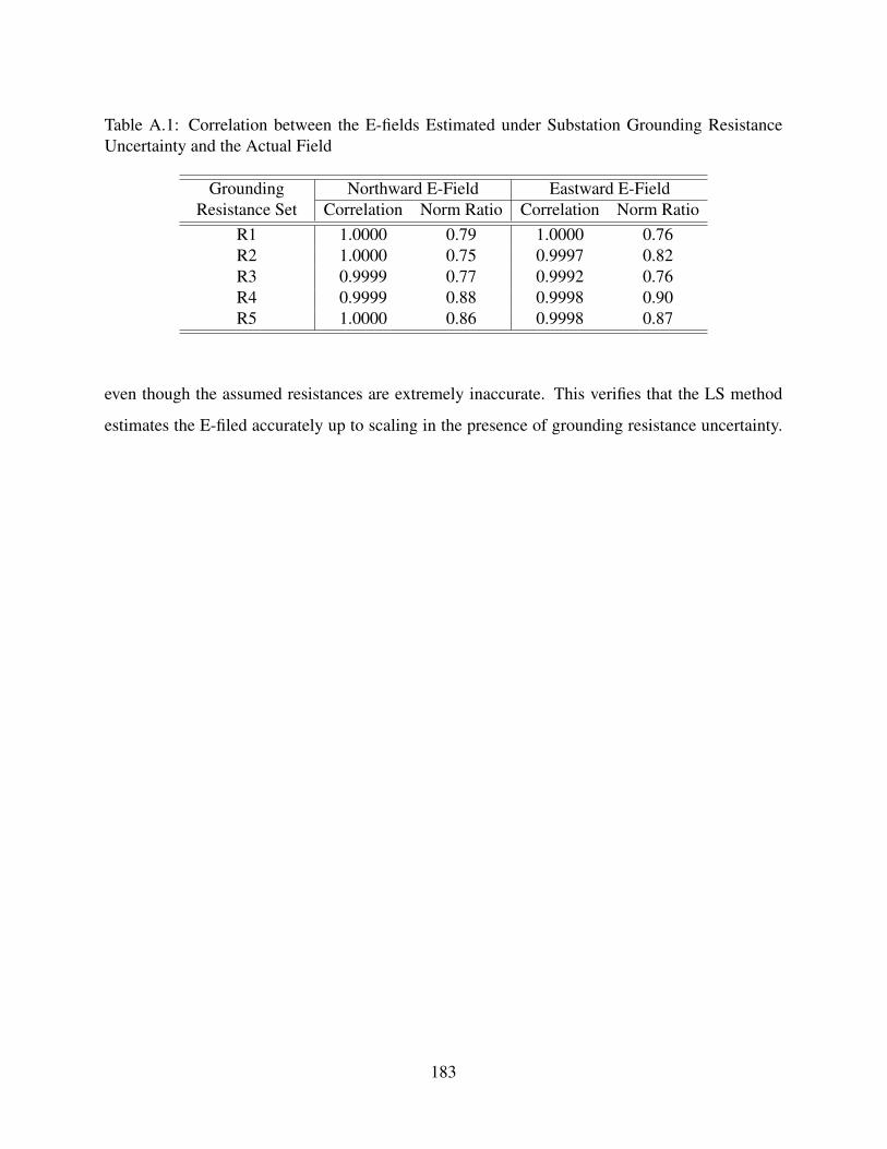
Table A.1: Correlation between the E-fields Estimated under Substation Grounding ResistanceUncertainty and the Actual Field
GroundingResistance Set
Northward E-Field Eastward E-FieldCorrelation Norm Ratio Correlation Norm Ratio
R1 1.0000 0.79 1.0000 0.76R2 1.0000 0.75 0.9997 0.82R3 0.9999 0.77 0.9992 0.76R4 0.9999 0.88 0.9998 0.90R5 1.0000 0.86 0.9998 0.87
even though the assumed resistances are extremely inaccurate. This verifies that the LS method
estimates the E-filed accurately up to scaling in the presence of grounding resistance uncertainty.
183

REFERENCES
[1] “2012 special reliability assessment interim report: Effects of geomagnetic disturbances onthe bulk power system,” North American Electric Reliability Corporation (NERC), Tech.Rep., Feb. 2012.
[2] “High-impact, low-frequency event risk to the north american bulk power system,” NorthAmerican Electric Reliability Corporation (NERC), Tech. Rep., Jun. 2010.
[3] “Electric power system resiliency: Challenges and opportunities,” Electric Power ResearchInstitute (EPRI), Tech. Rep., Feb. 2016.
[4] “IEEE guide for electric power distribution reliability indices - redline,” IEEE Std 1366-2012(Revision of IEEE Std 1366-2003), May 2012.
[5] “Severe impact resilience: Considerations and recommendations,” North American ElectricReliability Corporation (NERC), Tech. Rep., May 2012.
[6] “Economic benefits of increasing electric grid resilience to weather outages,” Executive Of-fice of the President, Aug. 2013.
[7] A. P. Meliopoulos and A. G. Bakirtzis, “Corrective control computations for large powersystems,” IEEE Transactions on Power Apparatus and Systems, vol. PAS-102, no. 11, pp.3598–3604, Nov. 1983.
[8] P. M. Anderson and B. K. LeReverend, “Industry experience with special protectionschemes,” IEEE Transactions on Power Systems, vol. 11, no. 3, pp. 1166–1179, Aug. 1996.
[9] C. F. Henville and E. Struyke, “Ras and streched power system,” Western Protective RelayingConference, 2006.
[10] “Special protection systems (SPS) / remedial action schemes (RAS): assessment of definition,regional practices, and application of related standards,” North American Electric ReliabilityCorporation (NERC), Tech. Rep., Apr. 2013.
[11] M. Varghese, L. Jin, S. Ghosh, G. Lin, and B. Pek, “The caiso experience of implementingautomated remedial action schemes in energy management systems,” in 2009 IEEE PowerEnergy Society General Meeting, Jul. 2009.
184
[12] J. Wen, W. H. E. Liu, P. L. Arons, and S. K. Pandey, “Evolution pathway towards wide areamonitoring and protection, a real-world implementation of centralized ras system,” IEEETransactions on Smart Grid, vol. 5, no. 3, pp. 1506–1513, May 2014.
[13] R. Ramanathan, B. Tuck, and J. O’Brien, “BPA’s experience of implementing remedial actionschemes in power flow for operation studies,” in 2013 IEEE Power Energy Society GeneralMeeting, Jul. 2013.
[14] S. C. Pai and J. Sun, “BCTCs experience towards a smarter grid - increasing limits and relia-bility with centralized intelligence remedial action schemes,” in Electric Power Conference,2008. EPEC 2008. IEEE Canada, Oct. 2008, pp. 1–7.
[15] A. A. Fouad, A. Ghafurian, K. Nodehi, and Y. Mansour, “Calculation of generation-sheddingrequirements of the B.C. hydro system using transient energy functions,” IEEE Power Engi-neering Review, vol. PER-6, no. 5, pp. 31–32, May 1986.
[16] Y. Zhang and K. Tomsovic, “Adaptive remedial action scheme based on transient energyanalysis,” in Power Systems Conference and Exposition, 2004. IEEE PES, Oct. 2004, pp.925–931 vol.2.
[17] I. Genc, R. Diao, V. Vittal, S. Kolluri, and S. Mandal, “Decision tree-based preventive andcorrective control applications for dynamic security enhancement in power systems,” IEEETransactions on Power Systems, vol. 25, no. 3, pp. 1611–1619, Aug. 2010.
[18] D. Ruiz-Vega and M. Pavella, “A comprehensive approach to transient stability control. ii.open loop emergency control,” IEEE Transactions on Power Systems, vol. 18, no. 4, pp.1454–1460, Nov. 2003.
[19] B. Gou and H. Zhang, “Fast real-time corrective control strategy for overload relief in bulkpower systems,” IET Generation, Transmission Distribution, vol. 7, no. 12, pp. 1508–1515,Dec. 2013.
[20] W. Shao and V. Vittal, “Corrective switching algorithm for relieving overloads and voltageviolations,” IEEE Transactions on Power Systems, vol. 20, no. 4, pp. 1877–1885, Nov. 2005.
[21] V. D. Albertson, J. M. Thorson, R. E. Clayton, and S. C. Tripathy, “Solar-induced-currentsin power systems: Cause and effects,” IEEE Transactions on Power Apparatus and Systems,vol. PAS-92, no. 2, pp. 471–477, Mar. 1973.
[22] J. Kappenman, “Low-frequency protection concepts for the electric powergrid:geomagnetically induced current (GIC) and E3 HEMP mitigation,” Oak RidgeNational Laboratory (ORNL), 2010.
[23] J. G. Kappenman, S. R. Norr, G. A. Sweezy, D. L. Carlson, V. D. Albertson, J. E. Harder, andB. L. Damsky, “GIC mitigation: a neutral blocking/bypass device to prevent the flow of GICin power systems,” IEEE Transactions on Power Delivery, vol. 6, no. 3, pp. 1271–1281, Jul.1991.
185

[24] H. Zhu and T. J. Overbye, “Blocking device placement for mitigating the effects of geo-magnetically induced currents,” IEEE Transactions on Power Systems, vol. 30, no. 4, pp.2081–2089, Jul. 2015.
[25] E. Arajärvi, R. Pirjola, and A. Viljanen, “Effects of neutral point reactors and series capacitorson geomagnetically induced currents in a high-voltage electric power transmission system,”Space Weather, vol. 9, no. 11, 2011.
[26] L. Bolduc, M. Granger, G. Pare, J. Saintonge, and L. Brophy, “Development of a dc current-blocking device for transformer neutrals,” IEEE Transactions on Power Delivery, vol. 20,no. 1, pp. 163–168, Jan. 2005.
[27] B. Kovan and F. de León, “Mitigation of geomagnetically induced currents by neutral switch-ing,” IEEE Transactions on Power Delivery, vol. 30, no. 4, pp. 1999–2006, Aug. 2015.
[28] J. G. Kappenman, “Mitigation of geomagnetically induced and dc stray currents,” EPRI Rep.EL-3295, Tech. Rep., 1983.
[29] A. A. Hussein and M. H. Ali, “Suppression of geomagnetic induced current using controlledground resistance of transformer,” Electric Power Systems Research, vol. 140, pp. 9 – 19,2016.
[30] J. G. Rolim and L. J. B. Machado, “A study of the use of corrective switching in transmissionsystems,” IEEE Transactions on Power Systems, vol. 14, no. 1, pp. 336–341, Feb. 1999.
[31] K. Hedman, R. O’Neill, E. Fisher, and S. Oren, “Optimal transmission switching with con-tingency analysis,” in IEEE PES General Meeting, Jul. 2010.
[32] A. A. Mazi, B. F. Wollenberg, and M. H. Hesse, “Corrective control of power system flows byline and bus-bar switching,” IEEE Power Engineering Review, vol. PER-6, no. 8, pp. 53–53,Aug. 1986.
[33] V. D. Albertson, J. G. Kappenman, N. Mohan, and G. A. Skarbakka, “Load-flow studies inthe presence of geomagnetically-induced currents,” IEEE Transactions on Power Apparatusand Systems, vol. PAS-100, no. 2, pp. 594–607, Feb. 1981.
[34] R. A. Walling and A. N. Khan, “Characteristics of transformer exciting-current during geo-magnetic disturbances,” IEEE Transactions on Power Delivery, vol. 6, no. 4, pp. 1707–1714,Oct. 1991.
[35] J. Kappenman, “Geomagnetic storms and their impacts on the U. S. power grid,” MetatechCorporation Report Meta-R-319, Tech. Rep., Jan. 2010.
[36] D. H. Boteler and R. J. Pirjola, “Modelling geomagnetically induced currents produced byrealistic and uniform electric fields,” IEEE Transactions on Power Delivery, vol. 13, no. 4,pp. 1303–1308, Oct. 1998.
186

[37] T. J. Overbye, T. R. Hutchins, K. Shetye, J. Weber, and S. Dahman, “Integration of geo-magnetic disturbance modeling into the power flow: A methodology for large-scale systemstudies,” in North American Power Symposium (NAPS), Sep. 2012.
[38] R. Horton, D. Boteler, T. J. Overbye, R. Pirjola, and R. C. Dugan, “A test case for the calcu-lation of geomagnetically induced currents,” IEEE Transactions on Power Delivery, vol. 27,no. 4, pp. 2368–2373, Oct. 2012.
[39] A. B. Birchfield, K. M. Gegner, T. Xu, K. S. Shetye, and T. J. Overbye, “Statistical consider-ations in the creation of realistic synthetic power grids for geomagnetic disturbance studies,”IEEE Transactions on Power Systems, 2016.
[40] R. Pirjola, “Properties of matrices included in the calculation of geomagnetically inducedcurrents (GICs) in power systems and introduction of a test model for gic computation algo-rithms,” Earth, Planets and Space, vol. 61, no. 2, pp. 263–272, 2009.
[41] A. Yan, D. Zhou, and L. Marti, “Analysis of geomagnetically induced currents,” in 2013IEEE Power Energy Society General Meeting, Jul. 2013, pp. 1–6.
[42] D. H. Boteler, A. J. C. Lackey, L. Marti, and S. Shelemy, “Equivalent circuits for modellinggeomagnetically induced currents from a neighbouring network,” in 2013 IEEE Power En-ergy Society General Meeting, Jul. 2013, pp. 1–5.
[43] R. Pirjola, “Study of effects of changes of earthing resistances on geomagnetically inducedcurrents in an electric power transmission system,” Radio Science, vol. 43, no. 1, 2008,rS1004.
[44] L. Marti, A. Rezaei-Zare, and D. Boteler, “Calculation of induced electric field during a geo-magnetic storm using recursive convolution,” IEEE Transactions on Power Delivery, vol. 29,no. 2, pp. 802–807, Apr. 2014.
[45] U. Bui, T. J. Overbye, K. Shetye, H. Zhu, and J. Weber, “Geomagnetically induced currentsensitivity to assumed substation grounding resistance,” in North American Power Sympo-sium (NAPS), 2013, Sep. 2013.
[46] “IEEE guide for measuring earth resistivity, ground impedance, and earth surface potentialsof a grounding system,” IEEE Std 81-2012 (Revision of IEEE Std 81-1983), pp. 1–86, Dec.2012.
[47] A. P. S. Meliopoulos, G. Cokkinides, H. Abdallah, S. Duong, and S. Patel, “A pc basedground impedance measurement instrument,” IEEE Transactions on Power Delivery, vol. 8,no. 3, pp. 1095–1106, Jul. 1993.
[48] F. Dawalibi and D. Mukhedkar, “Ground electrode resistance measurements in non uniformsoils,” IEEE Transactions on Power Apparatus and Systems, vol. PAS-93, no. 1, pp. 109–115,Jan. 1974.
[49] G. F. Thug, Earth Resistances. London: Georges Newnes Limited, 1964.
187

[50] F. Dawalibi and D. Mukhedkar, “Optimum design of substation grounding in a two layerearth structure: Part i, analytical study,” IEEE Transactions on Power Apparatus and Systems,vol. 94, no. 2, pp. 252–261, Mar. 1975.
[51] Z. Xu, J. L. Gannon, and E. J. Rigler, “Report of geomagnetic pulsation indices for spaceweather applications,” U.S. Geological Survey, Tech. Rep. 1166, 2013.
[52] U. Mersmann, W. Baujohann, F. Kuppers, and K. Lange, “Analysis of an eastward elec-trojet by means of upward continuation of ground-based magnetometer data,” Journal ofGeophysics, vol. 45, pp. 281–298, 1979.
[53] C. D. Beggan and S. A. McLay, “Interpolation of magnetic and electric fields using sphericalelementary current systems,” in Ionospheric Radio Systems and Techniques (IRST 2012),12th IET International Conference on, May 2012, pp. 1–5.
[54] M. Kazerooni, H. Zhu, K. Shetye, and T. J. Overbye, “Estimation of geoelectric field forvalidating geomagnetic disturbance modeling,” in Power and Energy Conference at Illinois(PECI), Feb. 2013.
[55] Synthetic Power Cases-Illinois Center for a Smarter Electric Grid. [Online]. Available:http://icseg.iti.illinois.edu/
[56] Power Systems Test Case Archives. [Online]. Available: http://www2.ee.washington.edu/research/pstca/
[57] G. D. Battista, P. Eades, R. Tamassia, and I. G. Tollis, Graph Drawing: Algorithms for theVisualization of Graphs, 1st ed. Prentice Hall PTR, 1998.
[58] U. Brandes, Drawing on Physical Analogies. Berlin, Heidelberg: Springer Berlin Heidel-berg, 2001.
[59] M. Kazerooni, H. Zhu, and T. J. Overbye, “Singular value decomposition in geomagneticallyinduced current validation,” in Innovative Smart Grid Technologies Conference (ISGT), 2015IEEE Power Energy Society, Feb. 2015.
[60] M. Kazerooni, H. Zhu, T. Overbye, and D. Wojtczak, “Transmission system geomagneticallyinduced current model validation,” accepted for publication in IEEE Transactions on PowerSystems, 2016.
[61] M. Kazerooni, H. Zhu, and T. J. Overbye, “Improved modeling of geomagnetically inducedcurrents utilizing derivation techniques for substation grounding resistance,” accepted forpublication in IEEE Transactions on Power Delivery, 2016.
[62] M. Kazerooni, H. Zhu, and T. J. Overbye, “Use of sparse magnetometer measurements forgeomagnetically induced current model validation,” in North American Power Symposium(NAPS), Oct. 2015.
[63] M. Kazerooni, H. Zhu, and T. J. Overbye, “Dynamic modeling and filtering in geomagneti-cally induced current validation,” in North American Power Symposium (NAPS), Sep. 2014.
188

[64] M. Kazerooni, H. Zhu, and T. J. Overbye, “Probabilistic modeling and reliability analysisfor validating geomagnetically induced current data,” in North American Power Symposium(NAPS), 2013.
[65] K. Stouffer, J. Falco, and K. Scarfone, “Guide to industrial control systems (ics) security,”NIST Special Publication, vol. 800, 2008.
[66] “A summary of control system security standards activities in the energy sector,” U.S. De-partment of Energy Office of Electricity Delivery and Energy Reliability, Oct. 2005.
[67] “NERC CIP 002 1 - critical cyber asset identification,” National Energy Regulatory Comis-sion, Tech. Rep., 2006.
[68] J. Weiss, “Are the NERC CIPS making the grid less reliable,” Control Global, 2009.
[69] S. Mohan, S. Bak, Y. E. E. Betti, H. Yun, L. Sha, and M. Caccamo, “S3a: Secure sys-tem simplex architecture for enhanced security and robustness of cyber-physical systems,”in Proceedings of the 2Nd ACM International Conference on High Confidence NetworkedSystems, 2013.
[70] S. Cheung, B. Dutertre, M. Fong, U. Lindqvist, K. Skinner, and A. Valdes, “Using model-based intrusion detection for scada networks,” in Proceedings of the SCADA Security Scien-tific Symposium, Miami Beach, Florida, Jan. 2007.
[71] W. M. Goble, Control Systems Safety Evaluation and Reliability. International Society ofAutomation, 2010.
[72] W. Shao and V. Vittal, “Corrective switching algorithm for relieving overloads and voltageviolations,” IEEE Transactions on Power Systems, vol. 20, no. 4, pp. 1877–1885, Nov. 2005.
[73] H. Ota, Y. Kitayama, H. Ito, N. Fukushima, K. Omata, K. Morita, and Y. Kokai, “Develop-ment of transient stability control system (tsc system) based on on-line stability calculation,”IEEE Transactions on Power Systems, vol. 11, no. 3, pp. 1463–1472, Aug. 1996.
[74] C. W. Taylor, F. R. Nassief, and R. L. Cresap, “Northwest power pool transient stabilityand load shedding controls for generation-load imbalances,” IEEE Transactions on PowerApparatus and Systems, vol. PAS-100, no. 7, pp. 3486–3495, Jul. 1981.
[75] S. M. Rovnyak, K. Mei, and G. Li, “Fast load shedding for angle stability control,” in PowerEngineering Society General Meeting, 2003, IEEE, Jul. 2003.
[76] G. Hug-Glanzmann and G. Andersson, “Decentralized optimal power flow control for over-lapping areas in power systems,” IEEE Transactions on Power Systems, vol. 24, no. 1, pp.327–336, Feb. 2009.
[77] A. R. Escobedo, E. Moreno-Centeno, and K. W. Hedman, “Topology control for load shedrecovery,” IEEE Transactions on Power Systems, vol. 29, no. 2, pp. 908–916, Mar. 2014.
189

[78] “D-FACTS devices in PowerWorld simulator.” [Online]. Available: http://www.powerworld.com/files/clientconf2014/07Weber\_DFACTS.pdf
[79] A. B. Birchfield, K. M. Gegner, T. Xu, K. S. Shetye, and T. J. Overbye, “Statistical consider-ations in the creation of realistic synthetic power grids for geomagnetic disturbance studies,”IEEE Transactions on Power Systems, 2016.
[80] V. D. Albertson, J. M. Thorson, and S. A. Miske, “The effects of geomagnetic storms onelectrical power systems,” IEEE Transactions on Power Apparatus and Systems, vol. PAS-93, no. 4, pp. 1031–1044, Jul. 1974.
[81] International Real-time Magnetic Observatory Network. [Online]. Available: http://www.intermagnet.org/
[82] G. B. Giannakis, G. Mateos, S. Farahmand, V. Kekatos, and H. Zhu, “USPACOR: Universalsparsity-controlling outlier rejection,” in 2011 IEEE International Conference on Acoustics,Speech and Signal Processing (ICASSP), May 2011, pp. 1952–1955.
[83] X. Dong, Y. Liu, and J. G. Kappenman, “Comparative analysis of exciting current harmonicsand reactive power consumption from GIC saturated transformers,” in IEEE Power Engineer-ing Society Winter Meeting, Jan. 2001.
[84] T. J. Overbye, K. S. Shetye, T. R. Hutchins, Q. Qiu, and J. D. Weber, “Power grid sensitivityanalysis of geomagnetically induced currents,” IEEE Transactions on Power Systems, vol. 28,no. 4, pp. 4821–4828, Nov. 2013.
[85] T. Guler, G. Gross, and M. Liu, “Generalized line outage distribution factors,” IEEE Trans-actions on Power Systems, vol. 22, no. 2, pp. 879–881, May 2007.
[86] F. L. Alvarado, “Computational complexity in power systems,” IEEE Transactions on PowerApparatus and Systems, vol. 95, no. 4, pp. 1028–1037, Jul. 1976.
[87] R. Yuster and U. Zwick, “Fast sparse matrix multiplication,” ACM Trans. Algorithms, vol. 1,no. 1, pp. 2–13, Jul. 2005.
[88] G. H. Golub and C. F. V. Loan, Matrix Computations, 3rd ed. Johns Hopkins, 1996.
[89] L. C. Liu, Y and R. Pirjola, “Observations and modeling of gic in the chinese large-scalehigh-voltage power networks,” J. Space Weather Space Clim., vol. 4, no. A03, 2014.
[90] NERC, “Benchmark geomagnetic disturbance event,” GMDTF Meeting, North AmericanElectric Reliability Corporation (NERC), Tech. Rep., Apr. 2014.
[91] “Special sensor ultroviolet spectrograph imager.” [Online]. Available: http://ssusi.jhuapl.edu/
[92] J. J. Leader, Numerical Analysis and Scientific Computation. Pearson Addison Wesley,2004.
[93] T. M. J. Fruchterman and E. M. Reingold, “Graph drawing by force-directed placement,”Softw. Pract. Exper., vol. 21, no. 11, pp. 1129–1164, Nov. 1991.
190

[94] T. Kamada and S. Kawai, “An algorithm for drawing general undirected graphs,” InformationProcessing Letters, vol. 31, no. 1, pp. 7 – 15, 1989.
[95] Power Systems Control and Automation Laboratory. [Online]. Available: http://pscal.ece.gatech.edu/archive/testsys/lines.html
191


