ET 438a Control Systems Technology

Laboratory 4Modeling Control Systems with MATLAB/Simulink

Position Control with Disturbances

Laboratory Learning Objectives

After completing this laboratory you will be able to:

1.) Convert differential equations representing an electromechanical control system into a block diagram with feedback.

2.) Use MATLAB Simulink software to represent a control system.3.) Implement a proportional and proportional-integral controller using Simulink

blocks.4.) Observe the effects of disturbances on feedback controller response.5.) Compare the responses of proportional and proportional-integral controllers with

respect to response time and steady-state error.

Theoretical and Technical Background

A well designed automatic control systems reduces the effects of outside system disturbances for a fixed set-point. A commonly encountered example of a control system that responds to outside disturbances is the cruise control found in automobiles. The driver establishes a cruising speed and the controller responds to changes in road conditions to maintain this desired value. One way to represent an outside disturbance is to consider it as an input to the system that adds to the system process load. This lab activity models an electromechanical antenna positioning system shown in Figure 1.

This figure shows a permanent magnet dc motor driven by an adjustable dc power supply adjusting the angular position of an antenna array. The desired position of the antenna as a function of time is given by A(t). The wind velocity produces a torque on the positioning shaft that is reflected to the motor shaft through a speed reducing gearbox. This gearbox reduces motor speed and increases motor torque allowing the motor to effectively use its mechanical power output to position the antenna array. A variable high-power dc power supply adjusts the motors armature voltage that, in turn, changes the antennas position through the gearbox. An automatic antenna controller takes a reference antenna position, sp(t) as an input. This is usually a constant with respect to time but may be a linear function for a tracking application.

Fall 2016 1 lab4_et438a.docx

Figure 1. Antenna Positioning System with External Wind Disturbance.

This lab activity uses MATLAB Simulink to compute antenna angle, A(t) for given disturbances caused by wind velocity changes using a block diagram model. The lab activity will implement proportional only control and proportional-integral control. Comparing the resulting antenna output position using these two types of controllers will demonstrate the advantages and disadvantages of each control mode.

Mathematical Modeling of the Positioning System-Dc Motor

This control system actuator is the armature-controlled permanent magnet dc motor. Figure 2 shows the dynamic model of the armature controlled motor. This model assumes that the motor drives a mechanical load directly from its shaft.

Figure 2. Armature–Controlled Dc Motor Model with Direct Load Drive.

The model parameter definitions are:

Fall 2016 2 lab4_et438a.docx

va(t) = armature voltage (V)ia(t) = armature current (A)eb(t) = motor back EMF (V)Tm(t) = motor developed torque (N-m)m(t) = motor shaft speed (rad/sec)TL(t) = mechanical load torque (N-m)Ra = armature resistance (Ohms)La = armature inductance (H)Bm = motor viscous friction (N-m-sec/rad)BL = load viscous friction (N-m-sec/rad)Jm = motor rotational inertia (kg-m2)JL = load rotational inertia (kg-m2)

This representation requires two more parameters to complete the model. These parameters are:

Ke = back EMF constant (V-sec/rad)KT = torque constant (N-m/A)

When using SI units (rad/sec and N-m) the numerical values of Ke and KT are equal. The follow system of equations represents the dynamic response of the motor speed to changes in armature voltage. In these equations, the motor armature current and the speed completely define the motor load response. The armature voltage and the load

dim( t )dt

=−(RaLa )⋅i a ( t )−(KeLa )⋅ω m ( t )+va( t )La

(a )

dωm( t )dt

=(KT(Jm+J L ) )⋅i a ( t )−((Bm+BL )(Jm+J L ) )⋅ωm ( t )−

T L( t )

(Jm+J L ) (b )

(1)

torque are the inputs to the system. Solving these differential equations, called state equations in control system theory, gives plots of motor armature current and speed with respect to time. Equation (1a) represents the electrical dynamics of the dc motor and includes an inductive time constant that restricts the rate at which current can change in the motor armature. Simulink uses equations in this form modified for numerical integration in a computer to produce response plots. Equation (1b) describes the mechanical dynamics. This equation includes a mechanical time constant represented by the ratio of total viscous damping (Bm+BL) to

Fall 2016 3 lab4_et438a.docx

total rotational inertia (Jm+JL). This ratio determines how quickly the motor/load speed can change.

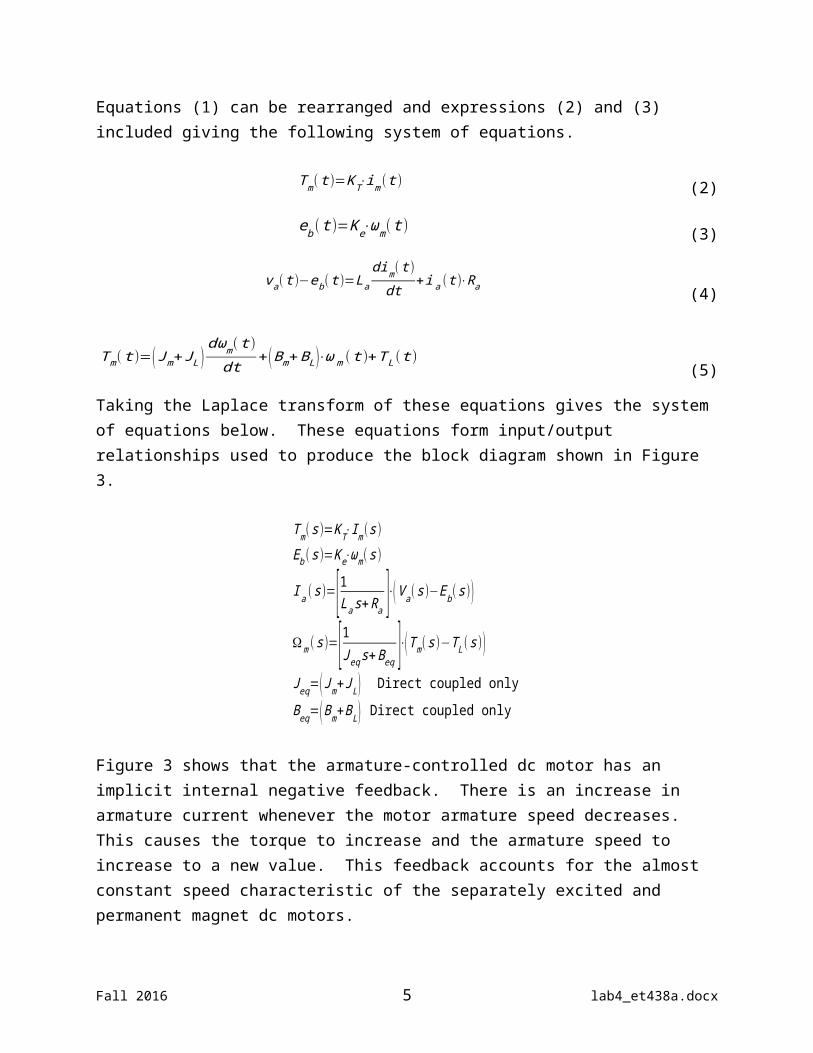
Equations (1) can be rearranged and expressions (2) and (3) included giving the following system of equations.

Tm( t )=KT⋅im( t ) (2)

eb ( t )=Ke⋅ωm( t ) (3)

va( t )−eb( t )=La

dim( t )dt

+ia (t )⋅Ra (4)

Tm( t )=(Jm+J L )

dωm( t )dt

+ (Bm+BL )⋅ωm ( t )+T L( t ) (5)

Taking the Laplace transform of these equations gives the system of equations below. These equations form input/output relationships used to produce the block diagram shown in Figure 3.

Tm(s )=K T⋅Im(s )Eb ( s )=Ke⋅ωm( s )

I a (s )=[1Las+Ra ]⋅(V a (s )−Eb (s ))

Ωm ( s )=[1J eq s+Beq ]⋅(Tm(s )−T L(s ))

Jeq=(Jm+J L ) Direct coupled onlyBeq=(Bm+BL) Direct coupled only

Figure 3 shows that the armature-controlled dc motor has an implicit internal negative feedback. There is an increase in armature current whenever the motor armature speed decreases. This causes the torque to increase and the armature speed to increase to a new value. This feedback accounts for the almost constant speed characteristic of the separately excited and permanent magnet dc motors.

Figure 3 shows that the difference between armature voltage and back EMF produces a voltage difference that determines the armature current. The values of La and Ra determine the magnitude and rate of change of this current. The torque constant

Fall 2016 4 lab4_et438a.docx

converts armature current into developed motor torque. Torque produces the motor shaft speed through the mechanical dynamics. The total viscous friction limits the motor

Figure 3. Block Diagram of an Armature-Controlled dc Motor with Direct Coupled Load.

speed while the total rotational inertia determine the rate of speed change.

This controller monitors the position of the antenna, so position must be related to the motor speed. Equation (6) uses the rate of change in position to express motor speed.

dθmdt

=ωm( t ) (6)

Where m = motor shaft position (rad)

This equation shows that integrating the speed of the motor shaft will give the motor shaft position. Figure 3 can then be modified to determine motor shaft position by adding integration to its output. Integration in the Laplace domain is division by the Laplace variable s. Figure 4 shows the motor model for armature voltage input and shaft position output.

Fall 2016 5 lab4_et438a.docx

Figure 4. Armature-Controlled Dc Motor with External Load and Shaft Position Output.

Equation (7) now shows the state equation representation for the dc motor with position output for a directly coupled mechanical load.

dim( t )dt

=−(RaLa )⋅i a ( t )−(KeLa )⋅ω m ( t )+va( t )La

(a )

dωm( t )dt

=(KT(Jm+J L ) )⋅i a ( t )−((Bm+BL )(Jm+J L ) )⋅ωm ( t )−

T L( t )

(Jm+J L ) (b )

dθm( t )dt

=ωm( t ) (c )

(7)

In most cases, the electrical time constant given by e=La/Ra is much smaller than the mechanical time constant m=Jm/Bm. This simplifies the transfer function and reduces the complexity of the mathematical model. If the ratio of the time constants, m/e ≥100 use the reduced order model given by equation (8) below.

Ωm( s )V a (s )

=K s1+ τ s⋅s

Where

K s=K TRa⋅Bm+K E⋅KT

τ s=Ra⋅JmRa⋅Bm+KE⋅K T (8)

The reduced model eliminates the torque summation node shown in Figure 4. A speed disturbance must now represent the wind torque disturbance. Figure 5 shows the block diagram for a reduced order motor model that has an external disturbance input.

Figure 5. Reduce Order Dc Motor Model with External load.

Fall 2016 6 lab4_et438a.docx

The mechanical dynamics given by the damping and rotational inertia of the external system transform a torque disturbance into a corresponding speed disturbance.

This version of the motor load model separates mechanical load parameters from the motor electrical parameters. The load rotational inertia and viscous friction are the parameters that convert the load torque into the load speed. The resulting motor-load speed produces a position change after integration.

The order reduction also removes the internal feedback loop between the internally generator voltage and the terminal voltage that controls the armature current. The block diagram shows the motor armature voltage controlling the motor speed directly through the first-order block.

Mathematical Model of Gear Systems

The antenna system motor drive couples to the antenna through a speed reducing gear system. The gear ratio changes the speed and torque values produced at the motor shaft. This ratio also changes the magnitude of the viscous friction and rotational inertia that the motor shaft sees. Figure 6 shows a representation of a simple gear drive comprised of two gears. The mechanical power source delivers speed

Figure 6. Speed, Torque and Position Representation For Gears.

1 and torque T1. The output is speed 2 and torque T2. The drive moves the input gear over 1 radians while the output gear moves over a distance of 2 radians. The radius of each gear determines the angular distances each gear covers per unit time. This also determines the angular speed. The gears cannot slip so the distance covered by the driven gear must equal the distance covered by the output gear. The following equation gives the length of arc covered per unit time in terms of the gear radius.

Fall 2016 7 lab4_et438a.docx

dθ1

dt⋅r 1=

dθ2

dt⋅r2 (9)

Where: r1 = radius of driven gearr2 = radius of output gear

The derivative of the angular displacement is the angular speed in radians/second. Also, the number of teeth in the gear is proportion to the radius.

Making these substitutions gives the following expression for speed change.

ω1⋅N1=ω2⋅N2ω1

ω2=N2

N1 (10)

Where N1 = number of teeth in the driven gearN2 = number of teeth in the output gear1 = drive speed2 = output speed

The position of the output gear shaft follows a similar relationship.

θ1

θ2=N2

N1 (11)

Where 1 = drive shaft position2 = output shaft position

The torque ratio is the inverse of the speed ratio. As the output speed decreases, the output torque increases for a fixed mechanical power input. This maintains a mechanical power balance across the gear box assuming no friction or other losses.

T2

T1=N2

N1 (12)

Where: T2 = output torqueT1 = drive torque

Gear boxes change the values of viscous friction and rotational inertia seen by loads and mechanical power sources. Figure 7 illustrates a typical mechanical system with viscous friction values B1 and B2 and rotational inertias J1 and J2 connected through a

Fall 2016 8 lab4_et438a.docx

gear box with N1 drive teeth and N2 output teeth. The gear ratio changes the values of mechanical output viscous friction and rotational inertia through the following formulas.

Jeqd=J 1+(N1

N2 )2

⋅J 2

Beqd=B1+(N1

N2 )2

⋅B2(13)

The parameters Jeqd and Beqd are the total equivalent rotational inertia and viscous friction seen from the drive side of the gear box.

Figure 7. Gear Box, Mechanical Load Inertias and Viscous Friction.

The gear ratio can change torque, speed, and position of the output shaft based on equations (10), (11) and (12). The following equations specify output speed torque and position in terms the drive variables.

ω1⋅(N1

N2)=ω2 (a )

θ1⋅(N 1

N 2 )=θ2 (b )

T 1⋅(N2

N1 )=T2 (c )(14)

When the output values are known, solve the above equations for the values of 1, 1 and T1 to get the equivalent speed, position and torque on the drive side of the gear box.

Fall 2016 9 lab4_et438a.docx

An ideal gear box is analogous to the ideal electrical transformer. Mechanical power is equal on both sides of the gear box. The gear ratio reduces speed but increases torque to maintain the power balance on both sides of the device. The parameters of viscous friction and inertia reflect through the gear box by multiply by gear ratio squared when viewed from the drive side of the device. These parameters are divided by the gear ratio squared when all quantities are referred to the output side of the gear box.

Position Sensing and Negative Feedback

Figure 8. Position Sensing and Error Generation.

Figure 8 shows the negative feedback loop required to generate an antenna position error signal. The position sensor monitors the antenna position and may amplify its output to scale it correctly for comparison with the set point position signal. The output of this block feeds to a summing junction that compares the measured position value to the desired value. An algebraic equation shown below describes this process.

K s⋅(θsp (s )−θm( s))=θe(s ) (15)

Where Ks = sensor gain (could be 1.0 to simplify model)sp(s) = setpoint value of antenna anglem(s) = measured value of antenna anglee(s) = angle error

When Ks=1.0 the output of the sensor is m(s) =A(s), the measured value equals the actual antenna position. The error angle provides the input signal to the controller that will then produce the correction signal for the dc motor/drive.

Control Mode Models

Three control modes exist for modifying the error signal of a negative feedback controller. The modes are proportional (P), integral (I) and derivative (D). Combining

Fall 2016 10 lab4_et438a.docx

these modes give several combinations of control response with differing characteristics. Commonly found combined modes include PI, PD and PID controls. Adjusting the constants associated with these combinations "tunes" the controller and modifies the system's response.

The proportional control mode takes the input error signal and amplifies it by a constant. Using this control mode may result in large amplification factors to achieve an acceptable steady-state error that can result in an unstable system. The integral control mode sums the error signal over time and can drive the steady-state error of a system to zero over time. The derivative control mode cannot be used alone since it only produces and output when the error input is changing. The derivative mode produces a correction signal based on the error's rate of change. This produces an anticipatory action that can improve a system’s stability. This lab activity will focus on proportional (P) control and proportional-integral (PI) control modes.

Figure 9 shows how to model the P and PI controller in Simulink. In these representations, Kp = proportional gain, KI = integral gain and s is the Laplace variable.

Figure 9. Simulink Block Diagram Models for P and PI Controllers.

The figure shows two alternatives for realizing the PI controller as a block diagram model. The first PI model uses a summing junction to combine the P and I actions while the second representation shows an algebraically reduced version using two cascaded blocks. The PI controller introduces a single pole in the system located as s=0 and a zero at s=-KI/Kp. Adjusting the values of Kp and KI modifies the system response and eliminates the steady-state error. In systems that already include an integrator, the addition of a pole at zero reduces the tracking error to zero. The antenna controller system includes an integral action in the conversion of motor shaft speed into shaft position. Using a PI control should produce a tracking error of zero after some time delay.

Negative Feedback and Disturbance Rejection

One of the benefits of utilizing negative feedback is that the controlled system tends to return to its desired value after encountering an outside disturbance on the output

Fall 2016 11 lab4_et438a.docx

signal. Figure 10 shows the block diagram of a system with a disturbance injected on the controller output. An external disturbance, D(s) acts on the system output, Y(s) to move the system from a stable value determined by the system setpoint, R(s). The overall response combines the influence of both inputs on the system.

Figure 10. Block Diagram of Negative Feedback With External Disturbance.

Superposition finds the overall output of the system taking R(s) and D(s) as individual inputs with the other input set to zero. Evaluating the resulting block diagrams for each individual input signal with the other input set to zero gives the output response produced by each input. The sum of the two outputs gives the total system response to both the disturbance and the setpoint.

Equation (16) shows how the set point and the disturbance signals contribute to the total output for a proportional controller with a gain of Kp.

Y ( s )=[ K p⋅G1( s )⋅G2( s )1+K p⋅G1( s )⋅G2( s )⋅H (s ) ]⋅R( s )+[ G1( s )

1+K p⋅G1( s )⋅G2( s )⋅H (s ) ]⋅D( s )(16)

This equation shows that if the value of Kp>>1, then the ratio multiplying R(s) approaches one. This means that the output will track the input with no steady-state error. The second term shows that for proportional gain, the magnitude of the disturbance diminishes as the value of Kp becomes very large.

Equation (17) shows the same relationship as (16) only with a proportional-integral (PI) controller used. The PI controller adds a pole at s=0 and a zero at s=-K I/Kp.

Fall 2016 12 lab4_et438a.docx

Y ( s )=[K p⋅(s+α )⋅G1( s )⋅G2( s )s+GH (s ) ]⋅R (s )+[s⋅G1(s )

s+GH ( s) ]⋅D( s )

WhereGH (s )=K p⋅(s+α )⋅G1 (s )⋅G2 (s )⋅H ( s )α=K I /K P (17)

Equation (17) has two parameters, Kp and KI, that control system response. Setting the zero of the PI control, which is the parameter =KI/Kp , to a value less than the dominant pole of the open-loop system changes the system performance. The dominant pole is the transfer function denominator polynomial root with the smallest numerical value, which is the longest time constant. This cancels some of the dominant pole’s effects and can increase the system response speed. Setting the value of controller zero at exactly the value of the dominate pole, in this case causes, the system to oscillate for all values of Kp. Setting the zero value to be greater than the dominate pole causes the output to be unstable. This analysis assumes the disturbance is zero.

The roots of the characteristic equation must all have positive negative real parts for system stability. The characteristic equation for the PI controller is given by

s+K p⋅(s+α )⋅G1( s )⋅G2( s )⋅H ( s )=0 (18)

Maintaining constant while adjusting Kp requires a change in KI. For a fixed zero location, then this relationship holds.

K I=α⋅K p (19)

For the PI controller selecting a value of and Kp will adjust the system response. Once a stable value of is found the value of Kp is adjusted to improve control performance.

Fall 2016 13 lab4_et438a.docx

Figure 11. Block Diagram of Antenna Positioning System Using a Full Armature Controlled Dc Motor Model and Proportional Controller.

Fall 2016 14 lab4_et438a.docx

Figure 12. Block Diagram of Antenna Positioning System Using Full Motor Dc Model and Proportional-Integral Controller

Fall 2016 15 lab4_et438a.docx

Figure 13. Antenna Positioning System Using a Reduced Order DC Motor Model and Proportional Controller.

Fall 2016 16 lab4_et438a.docx

Figure 14. Antenna Positioning System Using a Reduced Order DC Motor Model and Proportional-Integral Controller.

Fall 2016 17 lab4_et438a.docx

Lab 4 Procedure

The antenna positioning system shown in Figure 1 has the following parameters summarized in Table 1. Use these parameters to compute the values of the constants in the block diagrams shown in Figures 11 through 14.

Table 1- System Parameters

Parameter Parameter Description (Units) Parameter Value

La Motor Armature Inductance (H) 0.020Ra Motor Armature Resistance (Ohms) 4.0KT Motor Torque Constant (N-m/A) 0.14Ke Motor EMF Constant (V-s/rad) 0.14Bm Motor Viscous Friction (N-m-s/rad) 0.001Jm Motor Rotational Inertia (kg-m2) 0.001Kpwm DC supply voltage conversion constant 1N1 Motor Gear Tooth Count 25N2 Output Gear Tooth Count 6250BL Antenna System Viscous Friction (N-m-s/rad) 37.5JL Antenna System Rotational Inertia (kg-s2) 50

Part 1a: Proportional Controller with Detailed Motor Model

1. Use the parameters from Table 1 above to compute the constants in the block diagram shown in Figure 11. Enter the results of your calculations into Table A-1 in the appendix for later submission.

2. Open a Simulink model using MatLAB and construct the block diagram model of Figure 11 using this program. The setpoint input has the following graphical representation and mathematical description. Refer to the lab video presentations to see how to

θsp (t )=¿ {0 .5⋅t 0≤t≤1 ¿ ¿¿¿

Fall 2016 18 lab4_et438a.docx

construct this waveform using Simulink inputs. Use this input for all the following block diagrams in this lab.

3. Construct the torque disturbance shown in the block diagram using the following mathematical description and figure. This input is a square pulse of two seconds beginning at 5 seconds and ending at 7 seconds. It has a magnitude of 20 N-m.

TW ( t )=¿ {0 0≤t≤5 ¿ {20 5< t≤ 7 ¿ ¿¿¿

Refer to the lab video presentations to see how to construct this wave shape using Simulink inputs. Use this disturbance for all following lab simulations.

3. Connect the setpoint input and the disturbance inputs to the block diagram constructed using Simulink and set the value of Kp to 0.5 and the simulation stop time to 15 seconds.

4. Review the lab video presentation on multiplexed scope display. Set up a scope and a multiplexer to gather both the setpoint wave and the output wave simultaneously. Name the connections entering the multiplexer to match the signal source.

5. Set the scope to save its acquired data to the MatLAB workspace. View the video presentation that describes this process.

6. Run the antenna simulation for Kp=0.5 and review the results by double clicking on the scope icon in Simulink.

7. Download and save the MatLAB script file named lab4process.m to your computer or storage device. Add the path to this file’s location to the MatLAB environment.

8. Enter the MatLAB command window and type the script name exactly. MatLAB is case sensitive.

9. A prompt will appear asking for the value of Kp used for this simulation. Enter the correct value and hit enter.

10.The script produces two plots: A time plot of the system input and output on the same axis and an error plot with the maximum error listed and the time that it occurs.

11.Copy these plots to a Word document and save them for later review and submission.

Fall 2016 19 lab4_et438a.docx

12. Run the antenna simulation using Kp=1 and review the results by double clicking on the scope icon.

13.Enter the MatLAB command window and type lab4process on the command line to execute the script. Enter the value of Kp when prompted.

14.View the time plots produced and copy them to a Word document for later review and submission.

15. Repeat steps 12 to 14 for the following values of Kp: 2, 4, 8, and 16. Note how the value of Kp changes the maximum error.

Part 1b: Proportional-Integral Controller with Detailed Motor Model

1. Use the parameter values of Table 1 to compute the constants for the block diagram model shown in Figure 12 replacing the proportional controller with one of the PI controller structures shown in Figure 9. Use the same inputs as the previous model.

2. Set up a scope to capture the setpoint input and the controller output just as in Part 1a of this lab. Set the scope to save its data to the MatLAB workspace for more processing.

3. Set the value of Kp to 4 and the value of =0.889. Set the simulation time to 15 seconds and run the simulation.

4. Enter the MatLAB command window and type lab4process on the command line to execute the script. Enter the value of Kp when prompted, which should be 4 in this case.

5. View the time plots and copy them to a Word document for later review and submission.

6. Repeat steps 3 to 5 for =0.4 and 0.2. Maintain the value of Kp at 4 for these two simulations.

7. Repeat steps 3 to 5 for a=0.2 and Kp=8. Does this change the value of the maximum error?

8. Note the differences in the error between the proportional only and proportional-integral controllers performance.

Part 2a: Proportional Controller with Reduced Motor Model

1. Use the parameter values in Table 1 and the formulas for the reduced dc motor model to compute the constants Figure 13’s block diagram. Place the computed values into Table A-2 in the appendix for future submission.

2. Compute the ratio of the motor electrical to mechanical time constants m=Jm/Bm and e=La/Ra to the criteria listed in the lab theoretical and technical section: m/e≥100. Does this motor qualify for model reduction?

Fall 2016 20 lab4_et438a.docx

3. Use Simulink and construct this block diagram using the constants from step 1. Note that the antenna mechanical dynamics convert the disturbing torque into a speed through the inverse of the gear ratio. Use the same inputs as those in Parts 1a and 1b.

4. Set up a scope to capture the system input and output plots. View the instructional video that shows how to complete this task. Set the scope to save the simulation’s data points to the MatLAB workspace for later processing.

5. Set the simulation time for 15 seconds. Run simulations of the proportional controller using the reduced model and a Kp=0.5. View the results on the scope when the simulation ends.

6. Enter the MatLAB command window and type lab4process on the command line to execute the script. Enter the value of Kp when prompted, which should be 0.5 in this case.

7. View the time plots and copy them to a Word document for later review and submission.

8. Repeat steps 5-7 for Kp=1, 2, 4, 8, and 16. Note how changing the value of Kp affects the magnitude and time of the maximum error. Compare this to the full dc motor model response.

Part 2b: Proportional-Integral Controller with Reduced Motor Model

1. Change the Simulink model to include the Proportional-Integral controller shown Figure 14’s block diagram. All other constants should be the same as used with the proportional only controller of Part 2a. A scope should remain connected to the input and output points as in Part 2a. This scope should be set to save data to the MatLAB workspace for more processing.

2. Set =5.9, Kp=4, and simulation time to 15 seconds. Run the simulation and examine the scope output showing both the desired input and the position output. Does this system output appear stable or does it oscillate?

3. Enter the MatLAB command window and type lab4process on the command line to execute the script. Enter the value of Kp when prompted, which should be 4 in this case.

4. View the time plots and copy them to a Word document for later review and submission. Compare this to the proportional only controller output. Does the error stabilize for this configuration?

5. Repeat steps 2-4 for Kp=4 and =3 and 1. Note how changing the value of the parameter changes the system response. Compare these plots to those generated using the full dc motor model.

Fall 2016 21 lab4_et438a.docx

Lab 4 Assessment

Submit the following items and perform the listed actions to complete this laboratory assignment.

1. Compile the results of the Part 1a simulations in Table A-3 in the Appendix. Use the plots generated for error and system response to complete this table for each value of Kp listed.

2. Compile the results of Part 1b simulations in Table A-4 in the Appendix. Use the plots generated for error and system response to complete this table.

3. Compile the results of the Part 2a simulations in Table A-5 in the Appendix. Use the plots generated for error and system response to complete this table for each value of Kp listed.

4. Compile the results of Part 2b simulations in Table A-6. Use the simulation results to complete this table. Indicate if the response is stable or unstable by placing a S or U in the last column of the table.

5. Convert Appendix A into a pdf document and submit it to the Lab 4 assignment Dropbox in the course online materials.

6. Complete the online quiz associated with Lab 4 in the course online materials. Use all data and plots gathered and the lab handout as a reference during the quiz.

7.

Fall 2016 22 lab4_et438a.docx

Appendix ACalculations Summary and Simulation Results

Table A-1: Part 1a and1b Model Constants

Formula/parameter Numerical ValueBeq

Jeq

1/La

1/Jeq

Ra/La

Beq/Jeq

N1/N2

Table A-2: Part 2a and 2b Model Constants

Formula/parameter Numerical ValueBL

JL

Ks

1/JL

s

BL/JL

N1/N2

N2/N1

Table A-3: Part 1a Proportional Control Full Dc Motor Model Error Results

Kp Maximum Error Time of Maximum Error0.5124816

Table A-4: Part 1b Proportional-Integral Control Full Dc Motor Model Error Results

Kp Maximum Error Time of Maximum Error0.8890.4000.200

Fall 2016 23 lab4_et438a.docx

Table A-5: Part 2a Proportional Control Reduced Dc Motor Model Error Results

Kp Maximum Error Time of Maximum Error0.5124816

Table A-6: Part 2b Proportional-Integral Control Reduced Dc Motor Model Error Results

Kp Maximum Error Time of Maximum Error Stable/Unstable (S/U)5.93.01.0

Fall 2016 24 lab4_et438a.docx