1368 - DIW Berlin: Startseite · 1368 Deutsches Institut ... (PHBS) for years 2006 ... population...

Discussion Papers

Data and Model Cross-Validation to Improve Accuracy of Microsimulation ResultsEstimates for the Polish Household Budget Survey

Michal Myck and Mateusz Najsztub

1368

Deutsches Institut für Wirtschaftsforschung 2014

Opinions expressed in this paper are those of the author(s) and do not necessarily reflect views of the institute. IMPRESSUM © DIW Berlin, 2014 DIW Berlin German Institute for Economic Research Mohrenstr. 58 10117 Berlin Tel. +49 (30) 897 89-0 Fax +49 (30) 897 89-200 http://www.diw.de ISSN print edition 1433-0210 ISSN electronic edition 1619-4535 Papers can be downloaded free of charge from the DIW Berlin website: http://www.diw.de/discussionpapers Discussion Papers of DIW Berlin are indexed in RePEc and SSRN: http://ideas.repec.org/s/diw/diwwpp.html http://www.ssrn.com/link/DIW-Berlin-German-Inst-Econ-Res.html

http://www.diw.de/

http://www.diw.de/discussionpapers

http://www.ssrn.com/link/DIW-Berlin-German-Inst-Econ-Res.html

Data and model cross-validation to improve accuracy ofmicrosimulation results: estimates for the Polish

Household Budget Survey

Michal Myck, Mateusz Najsztub∗

March 26, 2014

Abstract

We conduct detailed analysis of the Polish Household Budget Survey data for theyears 2006-2011 with the focus on its representativeness from the point of view ofmicrosimulation analysis. We find important discrepancies between the data weightedwith baseline grossing-up weights and official statistics from other sources. A number ofre-weighting exercises is examined from the point of view of the accuracy of microsim-ulation results and we show that using a combination of demographic calibration tar-gets with several economic status variables or tax identifiers from the microsimulationmodel substantially improves the correspondence of model results and administrativedata. While demographic re-weighting is neutral from the point of view of incomedistribution, calibrating the grossing-up weights to adjust for economic status and taxidentifiers significantly increases income inequality. We argue that although data re-weighting can substantially improve the accuracy of microsimulation it should be usedwith caution.Keywords: microsimulation, re-weighting, household data analysisJEL Classification: D31, I38

∗Michal Myck (corresponding author) is Director of CenEA - the Centre for Economic Analysis in Szczecinand Research Fellow at DIW-Berlin (e-mail: [email protected]); Mateusz Najsztub is Research Economistat CenEA. Michal Myck gratefully acknowledges the support of the Polish National Science Centre (NCN)under project grant number 6752/B/H03/2011/40. Mateusz Najsztub acknowledges the support of theBatory Foundation under the project number 22078. Data used for the analysis have been provided by thePolish Central Statistical Office (GUS), who take no responsibility for the results of the analysis. The paperbuilds on the initial analysis conducted in the process of development of the SIMPL microsimulation model(version V4S) in cooperation with Adrian Domitrz, Leszek Morawski and Aneta Semeniuk. Their role in thedevelopment of the model has been indispensable. The usual disclaimer applies.

1

1 IntroductionThe majority of large scale household surveys conducted by statistical offices or private surveyagencies are conducted in such a way as to be “representative” of the population which therespective samples are drawn from. Due to frequent non-random survey participation thisrepresentativeness is usually less than perfect and the problems of under-representation ofcertain groups of the population - for example the very rich or the very poor - have been longrecognized. As we demonstrate using the example of the Polish Household Budget Surveys,if this under- or over-representation of certain groups is unaccounted for in the process ofgeneration of population grossing-up weights, the resulting population structure may differsubstantially from administrative records. This in turn has significant consequences for theaccuracy of tax and benefit simulations using a microsimulation model and thus the reliabilityof the model for the purpose of policy analysis (Klevmarken (2002)). Because validity ofany microsimulation model relies to a large extent on the degree of correspondence betweenmodel outcomes and the administrative records, significant deviations in terms of the ageor economic activity distribution and the resulting simulation discrepancies might lead toquestioning of the models’ role for policy purposes. In such cases even if model calculationsfor each particular household are correct, the grossed-up values are bound to be wrong.

We examine the data of the Polish Household Budget Surveys (PHBS) for years 2006–2011 from the perspective of tax and benefit microsimulation. The exercise presented in thispaper serves primarily the purpose of improving consistency of microsimulation results withadministrative data on aggregate tax burden and benefit expenditure. We are thus far fromeither questioning the general approach of the Polish Central Statistical Office (CSO) to thegeneration of PHBS grossing-up weights or from arguing that our approach should be appliedmore broadly in other applications of household micro-level data. We show, however, that arelatively simple method of data re-weighting along the lines of Gomulka (1992), Deville andSarndal (1992) and Creedy and Tuckwell (2004), which has recently been applied widely invarious types of micro-data analysis (e.g.: Brewer et al. 2009 and Navicke et al. 2013) cansignificantly improve the accuracy of tax and benefit microsimulations in many dimensions.We present an approach to calibration of population weights which extends the criteria usedby the CSO in several stages. In the first stage the calibration of weights is done withrespect to demographic variables.1 In the second stage we extend this to include economicstatus variables, while in the third we use a process of “cross-validation” where we calibratepopulation weights in the data with respect to a set of tax identifiers related directly tomicrosimulation. Naturally the latter approach relies on the assumption of the reliability ofthe basic model outcomes used for the calibration.

The second and third stage of this exercise generate significant improvements in terms ofthe performance of the tax and benefit microsimulation with respect to a chosen set of key taxand benefit parameters. The re-weighting exercise conducted in this paper demonstrates howa careful approach to household survey data may improve the accuracy of microsimulationof taxes and benefits thereby making the model much more applicable for policy analysis. In

1For re-weighting using age groups see: Cai, Creedy, and Kalb (2006).

2

the Appendix we extend our cross-validation approach further and make more extensive useof the outcomes of microsimulation to correct for the under-representation of high incomehouseholds using simulated values of tax advantages.

The rest of the paper is organised as follows. In Section 2 we briefly describe the PolishHousehold Budget Survey data used for the analysis including the sampling frame of thesurvey and the approach of the Central Statistical Office to the computation of populationweights provided with the data, referred to as “baseline” weights. Using these weights inSection 3 we present the differences in the age distributions between the baseline PHBS dataand other official sources on the demographic structure of the population as well as the corre-spondence of the economic status information in the data and administrative statistics. Thedivergence between these distributions forms the principal motivation for the weight calibra-tion in the paper. In Section 3 we show how these underlying differences find their reflectionin discrepancies of microsimulation results using a number of key tax and benefit parametersfrom the microsimulation model SIMPL which is applied to the PHBS data.2 The methodof weight re-calibration, which follows Gomulka (1992) and Creedy and Tuckwell (2004) isbriefly discussed in Section 4 including details on different stages of calibration. Results ofthe process in the form of a comparison of tax and benefit microsimulation outcomes withadministrative information is presented in Section 5. It should come as no surprise thatthe consistency of the grossed-up population structure in the data in terms of demographicsand economic activity has a substantial influence on the accuracy of microsimulation. Inter-estingly weight adjustments for economic activity status and tax identifiers have significantimplications for the level and trends in inequality indicators. Conclusions including somewords of caution regarding the methods applied in this paper follow in Section 6.

2 Polish Household Budget Survey dataThe Polish Household Budget Survey (PHBS) is an annual representative survey coveringin recent years over 37,000 Polish households. The first survey was conducted in 1957 andit has been a regular source of information on income, consumption and quality of life ofPolish citizens. Through the years it has undergone a number of more and less significantmethodological changes, related among other things to the political and economic transitionafter 1989 and various forms of standardization to international procedures, but the surveycontinues to collect detailed information on the household structure, income sources andhousehold expenditure. The information covered by the survey includes:

• socio-demographic composition of the household;

• life quality and housing conditions;

• durable goods and housing equipment;

• economic activity of household members;2For more details about the model see: Bargain et al. 2007 and Morawski et al. 2008.

3

• level and sources of individual and household-level incomes;

• detailed household expenditures.

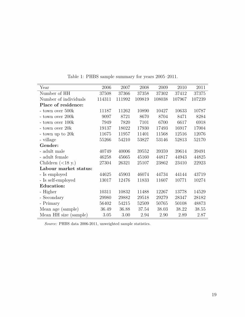
The PHBS methodology has changed over the years, but fieldwork procedures and theoverall methodology since 2006 has seen only minor modifications (Główny Urząd Statysty-czny (2011a)). In recent years the sample includes all households with the exception ofcollective dwellings such as prisons, cloisters, retirement homes or boarding schools. Thesampling methodology since 2006 targets 3132 of different dwellings in each month whichare selected for the survey giving a total of expected 37584 dwellings each year. Due to thepossibility of multiple households in one dwelling and survey interruptions (which are notreplaced with reserve households), the actual number of surveyed households may slightlydeviate from the target, as summarized in Table 1.

The data from the PHBS has been used in a number of studies of incomes and consump-tion and has long been the main survey used in the Polish microsimulation model SIMPL.3Most of the information collected in the PHBS, and in particular incomes and expenditures,covers the survey period of one month. For every quarter of the year each household beingsurveyed in that quarter is once again asked to fill a questionnaire regarding durable goodspresent in the household, as well as rare income and expenditure (e.g. buying or selling prop-erty, buying a car, health care services) and other sources of income such as employmentfringe benefits.

Table 1 HERE

Table 1 gives a summary of the number of households and individuals in the PHBS in theyears covered by the analysis, and the split at the household and individual level by somemain characteristics. Over the years we can observe the increasing number of people withhigher education and the higher (unweighted) average age of participants in the survey. Theaverage household size fell from over three individuals per household in 2006 to 2.87 in 2011.

2.1 PHBS sampling schemePHBS relies on a two-stage random sampling scheme with clustering and rotation (Lysoń(2012)). First the country is divided into around 30,000 Primary Sampling Units (PSUs)consisting of at least 250 dwellings in the urban areas and at least 150 dwellings in ruralareas. The PSU’s are clustered into 109 layers. 1566 PSUs are selected and divided to twosub-samples containing 783 PSUs each. Each sub-sample is drawn for two subsequent yearsand is exchanged every year forming two rotation groups. In the second sampling stage 24dwellings are drawn in each PSU (two for each month of the survey) together with additional150 reserve households in case of refusal of participation among the primary dwellings. Allhouseholds in every dwelling are included in the survey.

3For examples of analysis using the PHBS see for example: Brzeziński and Kostro (2010), Brzeziński(2010), Morawski and Myck (2010), Haan and Myck (2012), Myck, Kurowska, and Kundera (2013).

4

Importantly from the point of view of this analysis the sampling scheme determines theway observation weights are assigned to each household as the inverse of selection probabilityfor every household. These weights are then adjusted by post stratification based on the datafrom the National Census (2002 census used for years before 2010 and the 2010 census usedin later years). Stratification is based on 12 strata. The reference characteristics used toform the strata are the place of residence (rural or urban) and size of the household (single,2 persons, 3, 4, 5 and 6+ persons).4 No additional information on sex, age or education isincluded in the generation of sample weights. As we show below the resulting distribution ofeven such basic characteristics as age or economic status may as a result significantly differfrom the National Census data and other administrative records. While such discrepanciesmight not matter in many types of analysis they are of crucial importance from the point ofview of reliability and policy relevance of results from microsimulation studies which oftenpresent grossed-up population values of the elements of the tax and benefit system.

3 Grossed-up PHBS and other data sources on the Pol-ish population

Validation of survey data against other sources is notoriously problematic given various def-initional differences and the nature of the specific survey. Thus not only grossing-up weightsof the survey data will determine discrepancies between different sources of information. Inthis Section we present three types of variables from the PHBS which are set against otherdata sources in a validation exercise using the baseline grossing-up weights provided by theCSO (and derived along the lines outlined above). These three types of variables are:

• demographics: age, education, residence;

• economic status: employment, self-employment, pension and unemployment benefitreceipt;

• microsimulation output: aggregated tax and benefit values; the number of tax payersand benefit recipients.

The grossed up values of these variables from the PHBS together with the most appropri-ate counterpart information from other sources are presented in Tables 2, 3 and 4 respectively.The information used to validate the PHBS data derives principally from CSO’s StatisticalYearbooks based on alternative data sources (principally National Census data). Adminis-trative information on taxes, insurance contributions and benefits comes from published andonline statistics of the Ministry of Finance, the Ministry of Labour and Social Policy andthe Polish Social Security Institution (ZUS).5

4For discussion of stratified sampling see: Cameron and Trivedi (2005).5Information on age composition for 2006 and 2007 was taken from the CSO Demographic Yearbook

(Główny Urząd Statystyczny (2006 - 2007)). For the years 2008 – 2010 from population reports asof 30 June (Główny Urząd Statystyczny (2008 - 2010)) and for 2011 from the National Census report

5

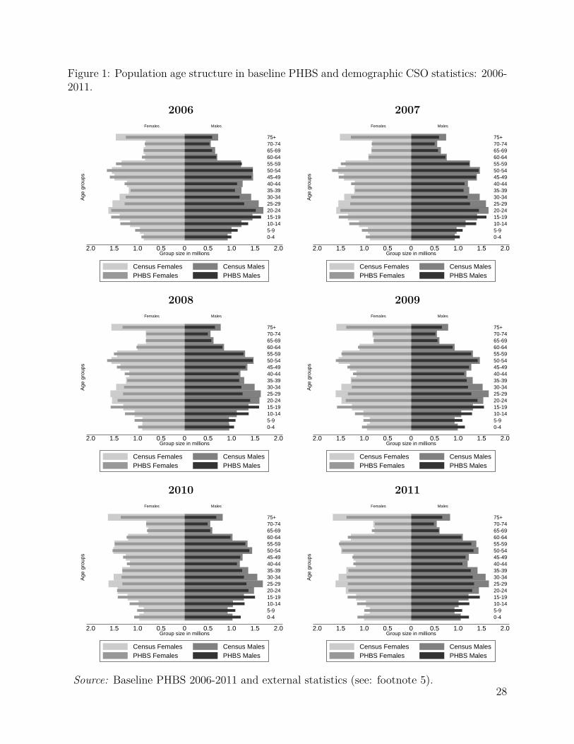
As we can see from Table 2 the gross-up population of Poland using the CSO baselineweights accounts for about 98-99% of the total population in the official statistics. Thissmall discrepancy is partly driven by lack of survey coverage of collective dwellings, butmay also be a result of small definitional differences concerning residence status betweensurvey and census data.6 More importantly though, a more detailed look at the populationdistribution by age suggests significant under and over-representation of some of the agegroups. Details for the years covered by the analysis are given in Figure 1 in the formof population pyramids by 5-year age groups. The dark-colored bars represent the PHBSpopulation, while the lighter colored ones the census-based official statistics. In all years weexamine we find over-representation of children and under-representation of those aged 20-49in the PHBS data relative to demographic statistics, both among men and women. There isalso some under-representation of the oldest groups of the population. Such difference in thedemographic structure of the population is to some extent surprising, in particular becausein this case there is little room for any definitional discrepancies. As we show below thesedifferences have significant consequences regarding the microsimulation of several importantelements of the tax and benefit system. This should not be surprising as many of theelements of the tax and benefit system, such as pensions or family benefits, are related tothe demographic composition of households.

FIGURE 1 HERE

Table 2 suggests also that the PHBS under-represents individuals with higher educationby about 20% relative to other sources, while in Table 3 we can see that relative to externalstatistics employees are over-represented in the sample by about 10% and the self-employedare under-represented in the more recent years of the data. In these cases there might be is-sues of definitional comparability of the different sources of data and of survey measurementerror. Some of the over-representation of employees may also arise from the fact that inthe data we cannot identify unofficial employment and thus treat all declarations of work at“face value” as official employment.7 Additionally people may confuse their employee/self-employed status given the popular forms of contracts between firms and single person enter-prizes. In these cases, in order to lower labor costs, while people are officially self-employed,

(Główny Urząd Statystyczny (2011)). Data on employment, pensions, education and place of residence canbe found in the Polish Statistical Yearbooks (Główny Urząd Statystyczny (2006 - 2011a) and Główny UrządStatystyczny (2006 - 2011b)). More details on pensions are obtained from the Social Insurance Institution(ZUS) reports (Zakład Ubezpieczeń Społecznych (2006 - 2011)). Information on Personal Income Tax wereobtained from the Polish Ministry of Finance reports (Ministerstwo Finansów (2006 - 2011)). Data on FamilyAllowance was taken from the Polish Ministry of Labour and Social Policy reports (Ministerstwo Pracy iPolityki Społecznej (2006 - 2011)), and data on health insurance and some detailed social security statisticsis taken from unpublished sources from ZUS - we are very grateful for making these available.

6For details see: Nowak (2013) and Główny Urząd Statystyczny (2011). The official statistics publishedin the Demographic Yearbooks are based on the 2002 and 2010 Census results which for the remaining yearsare updated with data from local administration registers.

7The number of people in the grey economy in 2010 was estimated to be around 800,000 (Główny UrządStatystyczny (2011b)), but many of these individuals could combine official and unofficial employment. It islikely that unofficial employment would not be declared in the survey.

6

they perform their tasks in the same way as an employee would. The PHBS data from yearsprior to 2010 significantly over-represent farmers which may be caused by definitional prob-lems in survey and administrative data, but probably reflects also the fact that weights priorto 2010 were based on the 2002 Farming Census and the structure of farming in Poland hasundergone substantial changes since then. The data beginning with 2010 with weights basedon the 2010 Farming and National Census are much closer to other administrative recordson the number of farmers in Poland. In Table 3 in addition to employment status compar-isons we also present the correspondence of the PHBS data with administrative records withregard to the number of recipients of the main Social Security benefits. The correspondenceof these numbers to official statistics differs in different years, but the number are generallyrelatively close. The main exception are Family Pensions, which are under-represented byup to 25%. The explanation behind this is that these pensions include survivors pensionswhich in the survey are likely to be declared by the surviving spouses as retirement pensions.This in turn might explain the over-representation of retirement pensions in the data.

Table 2 HERE

Table 3 HERE

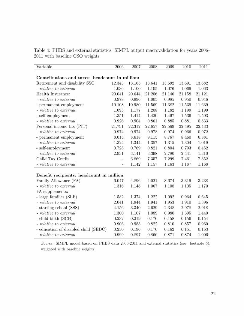
Table 4 HERE

The values presented in Table 4 compare direct output from the SIMPL microsimulationmodel to administrative statistics on the main elements of the tax and benefit system. Wepresent the simulated number of individuals contributing to Social Security (SSC), HealthInsurance (HI) and Personal Income Tax (PIT), and the number of recipients of FamilyBenefits including the principal Family Allowance (FA) and four main supplements (forlarge families: SLF, for starting school: SSS, for child birth: SCB, and education of disabledchildren: SEDC). In the case of each year we use the SIMPL microsimulation model tosimulate the baseline tax and benefit system which operated in that year. Within the HI andPIT categories we show the total number of contributors and additionally list the numbersby those paying contributions on permanent employment and self-employment income. ForPIT we also give the numbers of recipients of the Child Tax Credit, a generous tax credit forfamilies with children introduced in 2007. The simulations of Social Security contributionsare relatively close to the official figures, with overestimate of 6.3% in 2011. Similarly to theoverall employment status we overestimate Health Insurance contributions for the employees(by between 2% and 20% ) and underestimate them for the self-employed (by 6% - 17%).The number of people paying income taxes, on the other hand, overall match relatively wellwith administrative statistics. However, since we are unable to account for the details of taxdeductions among the self employed, and cannot identify clearly the specific ways people filetheir taxes, the number of tax payers in this category is substantially higher compared to theofficial statistics. Given the over-representation of children in the data it is not surprisingthat the model significantly overestimates the number of recipients of the Child Tax Creditas well as the means-tested Family Benefits. In the latter case the basic Family Allowance

7

is overestimated by about 32% in 2006 and by 17% in 2011, while the supplement to largefamilies by as much as 104% in 2005 and 40% in 2011. These figures suggest that whilethe data generally over-represent families with children, it might be over-representing thehouseholds with a high number of children to a much larger degree than households withone or two children.

4 Weight calibrationIn this Section we present the approach we take to calibration of weights applied to thePHBS data. In the exercise the primary source of external data with respect to which thebaseline weights are calibrated is information on demographics and employment status. Thisis then supplemented with information on income sources and finally with a small numberof variables simulated in the microsimulaiton model. The weight calibration exercise followsthe approach of Vanderhoeft (2001) and Creedy (2004) described also in Deville and Sarndal(1992).

The main principle of the approach is that it assumes validity of the “target” data towhich the weights are calibrated. In our case, in the first stage it implies the fact that wetrust the external information on the age distribution, while in the second also the data onlabor market and income status. In the final stage the assumptions also imply that we trustthe procedures applied in the tax and benefit model in that they correctly identify thosewho pay the “target” taxes.

The calibration procedure does not change the observations themselves. Instead, itchanges the household weights in such a way as to represent different aggregated popu-lation characteristics in the best possible way, taking into account a “minimum-distance”criterium which minimizes the sum of differences between the old and new weights. Thegeneral idea is the following. Having m variables and n observations, we have a vector xjk,where j = 1, 2, . . . , m and k = 1, 2, . . . , n. We can then define population totals for everyvariable tj such that tj = ∑n

k=1 dkxjk, where dk are the initial (baseline) weights.The goal of the exercise is to minimise the distance wkG(·), where G(·) is a distance

function:minwk

n∑k=1

wkG(

wk

dk

)(1)

subjected to m calibration constraints:n∑

k=1wkxjk = t′

j, j = 1, 2, . . . , m (2)

where wk are the new calibrated weights equal to wk = gkdk, with gk representing thefactors by which baseline weights are adjusted, and t′

j are the target population totals, setas targets for the calibration exercise.

Different distance functions can be used for the calibration procedure. The approachused here follows the Deville-Sarndal distance function described in Deville and Sarndal(1992) that eliminates negative weights and constrains the new weights not to exceed a

8

specified lower and upper bound, relative to the old weights. The optimization problem (1)constrained by (2) is solved numerically using the Lagrange multipliers method. More detailson finding the solution and properties of different distance functions can be found in Devilleand Sarndal (1992), Vanderhoeft (2001) and Creedy (2004). Calibration procedure accordingto the above methodology is available in Stata in the REWEIGHT package of Pacifico (2010).The Deville and Sarndal (1992) distance function allows setting the minimum and maximumfactors by which new weights may differ relative to the old ones, and the package permitsautomatic adjustment of these values once the initial factors prove too restrictive for theiterative algorithm.

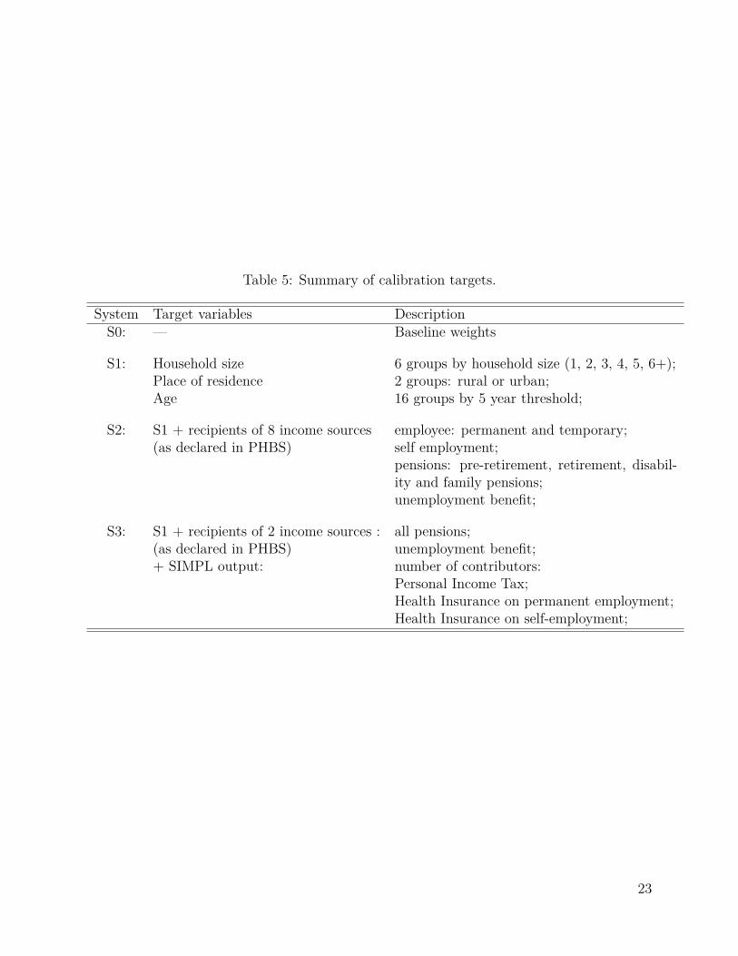
4.1 Three stages of calibrationThere is clearly an endless number of ways in which weight calibrations could be conducted,conditional on the choice and number of target variables as well as specific methods ofcalibration. In this paper we conduct the calibration exercise in three stages in each caseusing the same set of target variables and the same calibration method for every year ofdata. The target variables used at each stage of calibration are given in Table 5.

Table 5 HERE

In each of the three calibration stages we target two principal variables which underliethe generation of baseline weights at the CSO in order for the calibration exercise not todiverge from these basic criteria. Thus we target household size (6 categories) and the placeof residence (2 groups). These three target variables are generated from the data using thebaseline weights so that they remain unchanged in the calibration exercise. The additionalcriterion on which weights are calibrated in stage 1 (S1) are demographic targets related tothe age distribution. In this case the target variables are the official population statisticsfrom Demographic Yearbooks by age group.8 Stage two (S2) extends these targets by addingseven types of basic income sources as declared in the PHBS, while in stage three (S3) we usetwo indicators for income receipt (any social security pension and unemployment benefit)and supplement this by a number of outcome variables from the SIMPL microsimulationmodel. These variables relate to the number of individuals paying Personal Income Taxand employee and self-employed Health Insurance. The starting weights for the calibrationexercise are the baseline weights as provided by the CSO. Results generated using theseweights are labelled as S(0).

A note of caution is necessary before we discuss the results. As we noted above thereis an endless number of weight calibrations one could conduct and there is no obvious orobjective criterion one should target. The calibrations presented in this paper aim primar-ily at finding a practical solution to the problem of under or over-representation of certaingroups of the population with respect to data which form a point reference for the purpose

8These need to be proportionally rescaled in order to keep the grossed-up population in the PHBS dataunchanged. For the full set of references to external statistics see footnote 5.

9

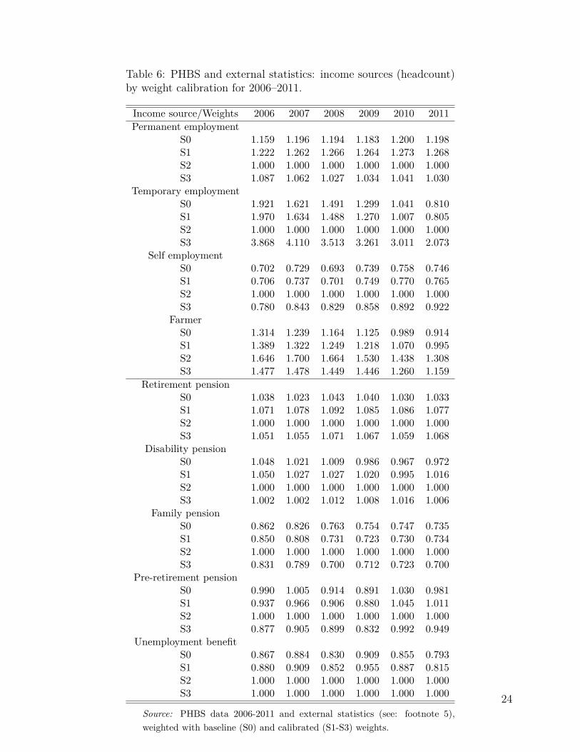
of microsimulation. We must also remember that there is a limit to the accuracy of cali-bration and to the number of target variables one can choose, as with too large a numberof targets the algorithm may not converge. We thus start from the most basic correctionof the discrepancies between the grossed-up survey data and other official statistics, namelythe age distribution. As we shall see already this change brings in a significant improvementin the accuracy of a number of simulation outcomes. The next two stages of calibrationsaim more specifically at adjusting the distribution with respect to the representativenessof households by the type and level of taxes and benefits they pay. In stage two of thecalibration process (S2) the target variables are economic activity categories defined by thesource of external income - i.e. income which is not simulated in the microsimulation. Thiscovers market incomes from employment and self-employment and social security benefitssuch as different types of pensions and unemployment benefit. Because it is unclear if theadministrative statistics on employment and self employment correspond to the economicstatus variables in the survey, in the third calibration stage we replace this by the number ofthose who pay income tax and health insurance while keeping the total number of pensionersand recipients of unemployment benefit as target variables. The principal reason behind thisis to ensure consistency of definitions between administrative and survey data since we nolonger need to distinguish between the source of income as long as it is subject to incometax. One argument against this type of approach might be that we may rely too much on thecorrect nature of the identification of the tax contributors and if these are wrong introducean erroneous target variable for the calibration procedures. In our view because we targetonly the number of those paying taxes and health insurance contributions and not its values,the scope for introducing such error is very small and as we shall see in the case of severaloutcome variables the advantages in terms of the accuracy of simulations are substantial.

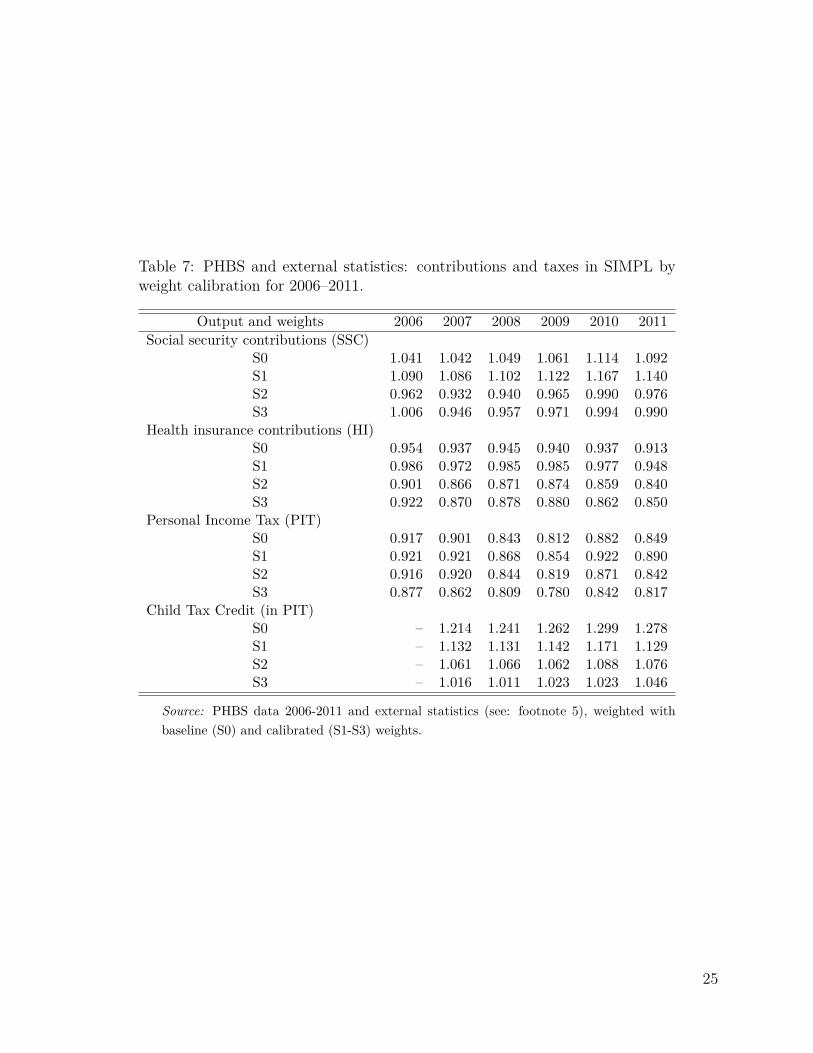
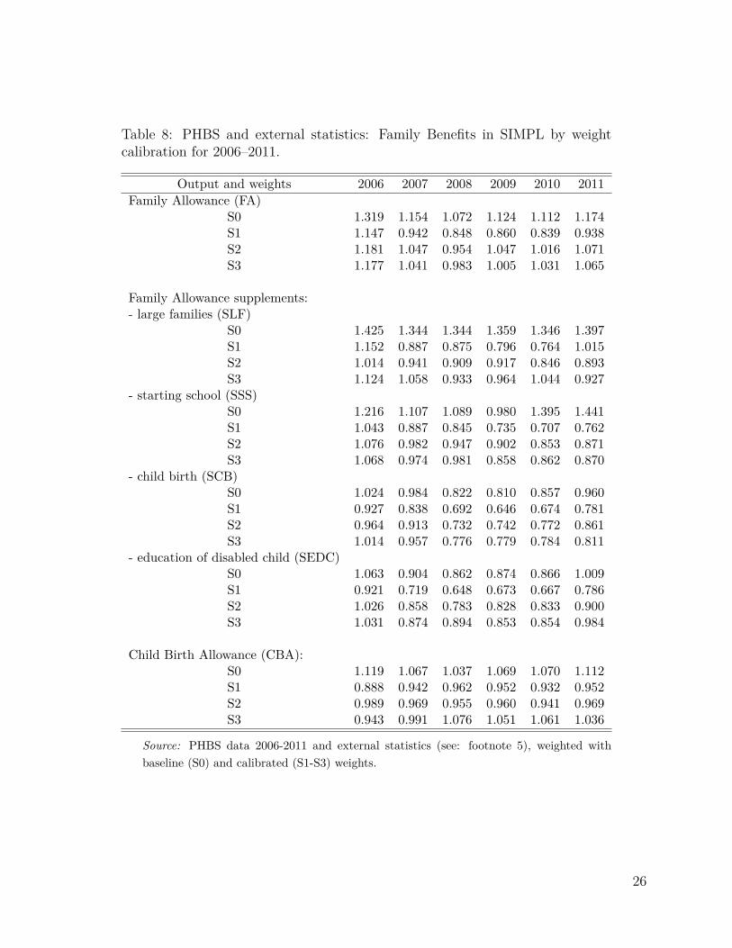
5 ResultsThe effect of weight calibration under the above three scenarios is presented in two separatecategories. First we show how the calibrations affect the correspondence of economic statusand social security benefit receipt relative to external data, and secondly we present aggregateoutcomes of the microsimulation model as compared to administrative statistics. In thisway one can immediately see the effect on the distribution of economic status and on theaccuracy of simulations relative to administrative data. In a similar way to the detailedresults presented in Table 4 for each of the years considered in the analysis we apply thebaseline tax and benefit system for the given year. The differences in the grossed-up numberof individuals in specific economic status and SSC benefit receipt category as well as withregard to the simulation outputs between S(0) and S(1)-S(3) result purely from changes inthe values of grossing-up weights. The results in the form of ratios of PHBS based figures andexternal sources for the economic status and SSC benefit receipt are presented in Table 6.The headcount figures for the simulated contributions and tax outcomes are shown in Table 7,while for Family Benefits outcomes in Table 8. For these parameters we also show the ratiosbetween the simulated and administrative information for headcount and aggregate amounts

10

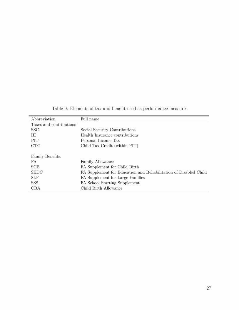
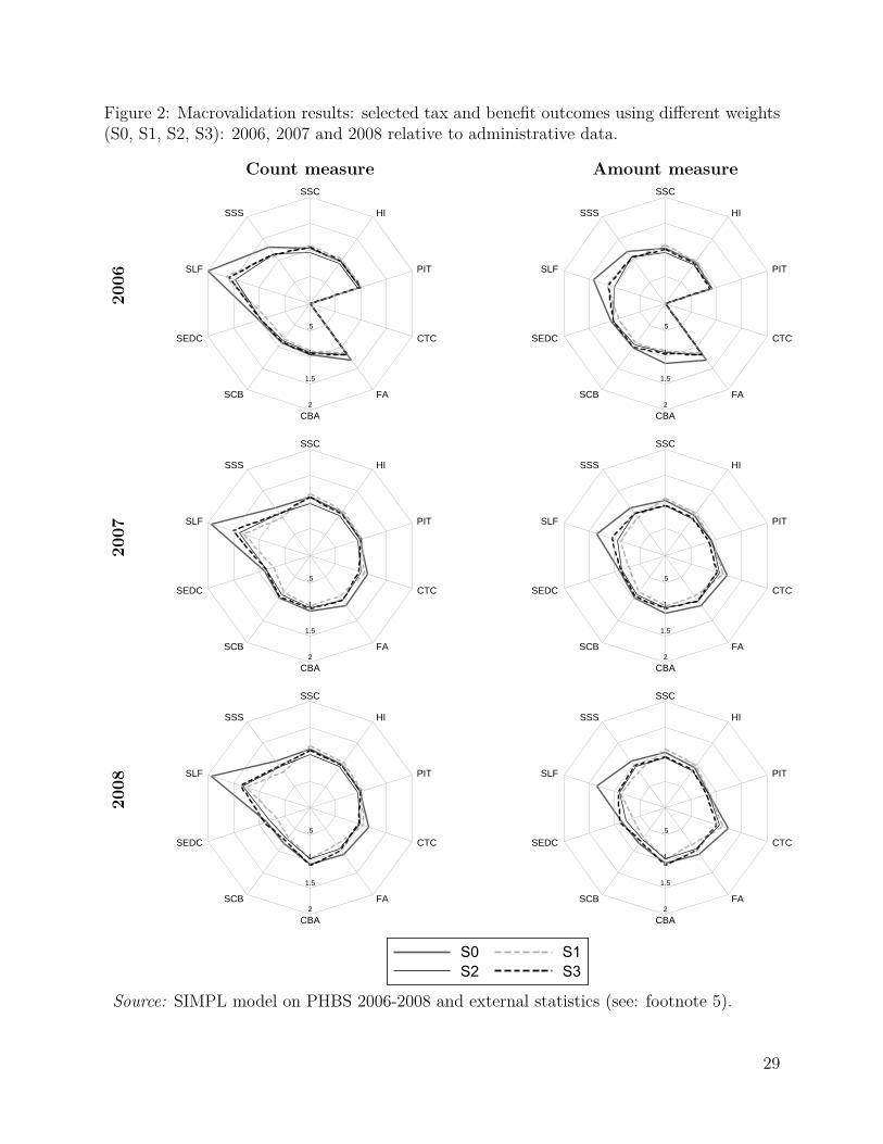
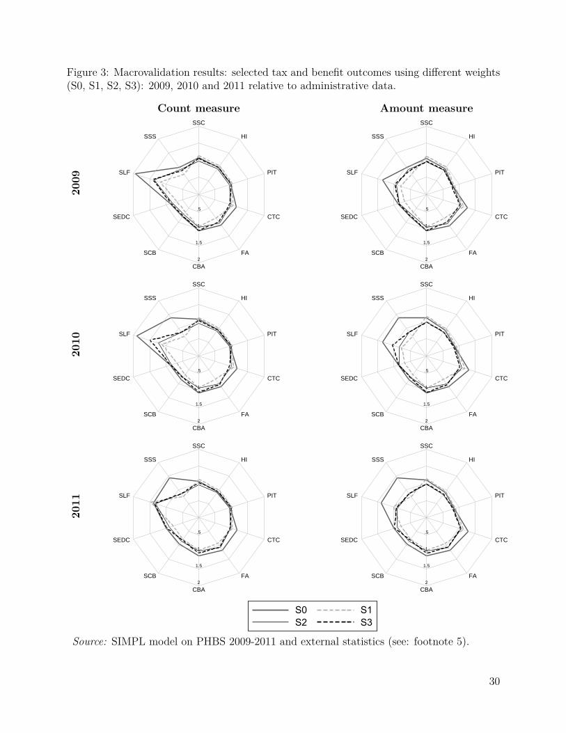
in the form of radar charts in Figures 2 and 3.9 The Tables and Figures include the same taxand benefit outcomes as those chosen for the baseline validation presented in Table 4. Thecloser the relative values are to 1, the closer are the simulated values to their administrativecounterparts. The list of the tax and benefit parameters and their labels is given in Table 9.

Table 6 HERE

Table 7 HERE

Table 8 HERE

Table 9 HERE

FIGURE 2 HERE

FIGURE 3 HERE

As shown in Tables 7 and 8 and summarized in Figures 2 and 3, weight calibration gen-erally leads to an improved correspondence in the results for most of the selected simulatedparameters. The most significant improvements apply to the Family Allowance and its sup-plements. The biggest relative deviation from the administrative data can be observed inthe Supplement for Large Families (SLF) which is oversimulated by nearly 100% in 2006 interms of the headcount measure and by 43% in terms of amount when using the baselineweights. For all calibration targets in the given period the number of recipients and theaggregate value of the SLF drops substantially and gets closer to the administrative records.The headcount values are still oversimulated but by much less compared to the baselineweights. In terms of total spending most of the simulations generate results closely match-ing the administrative values. A similar picture can be seen for the Supplement for StartingSchool (SSS) in years 2010 and 2011.

The results on the contributions side are not as straightforward, and there are importantdifferences between the accuracy of results by headcount and aggregate amounts. Figures 2and 3 show that, as we would expect given the target variables in S2 and S3, the second andthird stage of the calibration substantially improve the respective number of contributors toSocial Security and Health Insurance and taxes. This is the result of calibrating the numberof recipients of the main types of incomes in S2 and of selected types of contributions in S3.The improvements in terms of aggregate amount of contributions and taxes, however, areless clear cut. The details are presented in Table 7 and we can see that generally while thereare improvements in terms of the numbers of contributors to Social Security, both S2 and S3calibrations result in higher deviations in terms of Health Insurance amounts taxes, althoughthese deteriorations are usually small in magnitude. The reason behind this is that targetingthe working population through either income sources or contributions, lowers the weight onmarket incomes and in particular assigns lower weights to top income recipients in the data

9These are generated using radar graphs for Stata (Mander (2007)).

11

who generate a significant proportion of tax and contributions incomes. In the Appendix wepropose an alternative calibration approach which directly uses microsimulation output tore-weight high income households and as a result produces a further correction to the overallvalues.

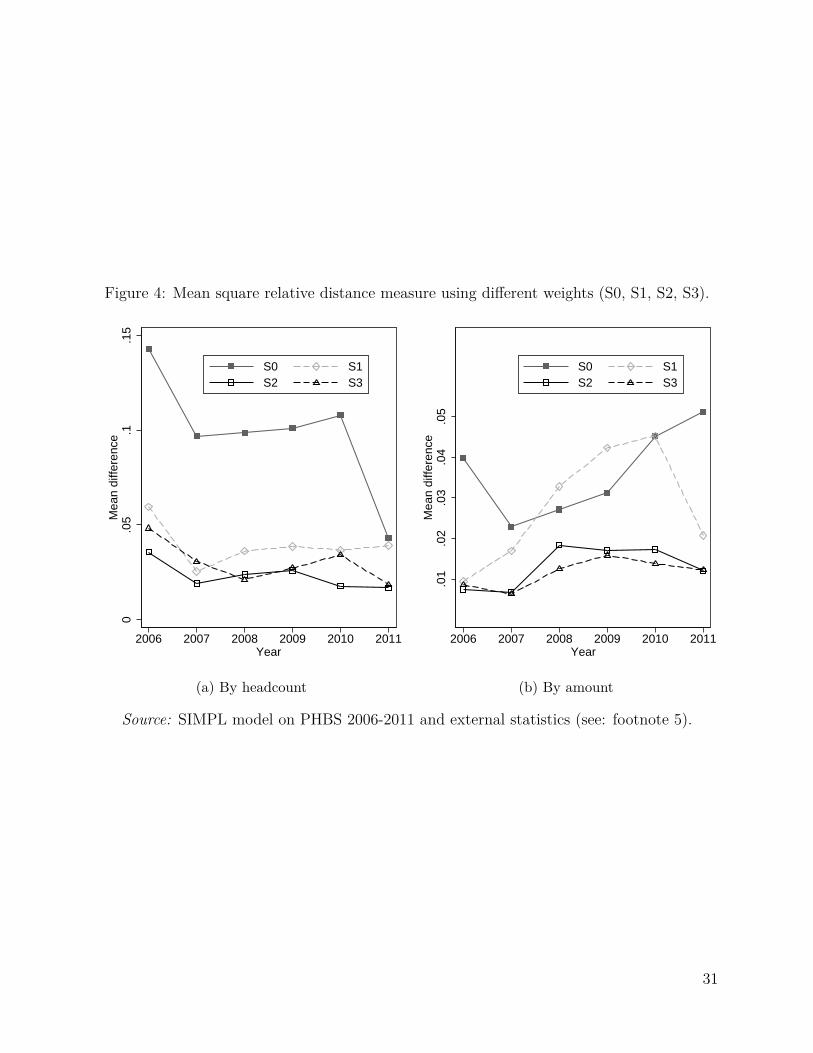
The accuracy of calibrations is summarized through a simple indicator covering the corre-spondence of the selected tax and benefit parameters. This is computed as the total squaredrelative deviation of the simulated values from administrative data:

d = 1l

l∑i=0

(1 − si)2 (3)

where l is the number of tax and benefit outcomes included in the analysis (as presentedin Table 9), and si is the ratio of simulated to administrative values for that particularoutcome. These indicators are computed separately for the headcount measure and foraggregate amounts of taxes and benefits. The summary of the comparison for the chosen setof parameters is presented in Figure 4. The summary results reflect our detailed discussionabove and overall for the second and third calibration stages show improvements in theaccuracy of simulations - even despite the less precise results on insurance and income taxesin some cases. The only case when the indicator with calibrated weights is higher comparedto the baseline is in the case of amounts for S1 calibrations in 2008 and 2009. These resultsrelate to a substantial undersimulation of a number of elements of the Family Benefits systemin these two years. It is interesting to note that the summary indicators for the second andthird stage of calibrations are very close to each other for all of the analyzed years in termsof both the headcount and aggregate amounts.

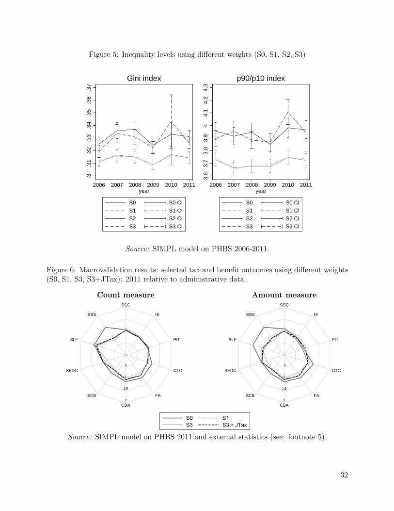
Finally, on top of the comparison of the headcount and aggregate amounts we also analysethe extent to which changes in grossing-up weights get reflected in inequality statistics. Onecould expect that changes in the composition of the population generated by the alternativeweights would result in changed distributions of income, and it is interesting to examinewhether the approach to weight calibration affects the trends in income inequality underdifferent calibration scenarios. Inequality statistics - the Gini coefficients and the 9/1 decileratios, together with their 95% confidence intervals, are shown in Figure 5.10 Differences ininequality measures when calibrating only to age groups are insignificant when compared tothe system with baseline weights. This is not the case with the two extended systems. Inboth cases inequality indicators are substantially higher and the differences with respect tothe measures using baseline weights are statistically significant.

FIGURE 4 HERE

FIGURE 5 HERE10To compute inequality statistics we use Inqdeco by Jenkins (1999). Confidence intervals are generated

using bootstrapping with 1000 draws.

12

6 Conclusions and notes of cautionAs we saw in Section 5 calibration of grossing-up weights by demographic characteristics(S1) and indicators related to the economic status (S2) and tax identifiers (S3) results insubstantial improvements in the accuracy of microsimulation results on the side of taxesas well as benefits. Interestingly major gains in the performance of the microsimulationmodels appear already after correcting for the distribution of age, which is probably theleast controversial and arbitrary adjustment, and these changes are neutral from the pointof view of the overall income distribution. The latter two stages of calibration significantlychange the distribution of income as reflected in inequality measures, although both of theseforms of re-weighting bring additional benefits in terms of accuracy of microsimulation.

There are several reasons why one should approach re-weighting of data with caution, andthey apply particularly strongly to the more sophisticated calibrations which are necessarilybased on a number of subjective and to some extent arbitrary choices made in the process.When considering the re-weighting procedures one first of all has to bear in mind the reasonsfor the discrepancies between the grossed-up population on the basis of the survey data andexternal statistics. In the least controversial cases, as in our case the distribution of age,we can count on reliable and directly comparable external data. The most likely reasonfor discrepancies in such cases is the selective survey non-response with respect to thesecharacteristics and the fact that the baseline weights do not account for them sufficiently.Adjusting the grossing-up weights in such cases, in particular if it also accounts for categoriestaken into consideration in generating the baseline weights, seems justified, and as we sawin Section 5 it might bring substantial gains in the accuracy of simulation results.

Discrepancies between survey and external data might however result also for other rea-sons. These include survey reporting errors (e.g.: Giles and McCrae (1995) and O’Donoghue,Sutherland, and Utili (1999)), definitional differences between survey and external data, aswell as in the case of comparisons of tax and benefit values, the issues of computationalaccuracy of the microsimulation model. For the latter reason one ought to approach the useof microsimulation output data for the purpose of re-weighting with a lot of caution. In thecase presented in this paper in the third stage of calibration we rely purely on identificationof individuals contributing to taxes and health insurance rather than calibrating specificbenefits or values of tax amounts.11 A clear example of a survey reporting error which wecould see in the above analysis is the likely confusion of retirement and survivor pensions,which in the Polish data leads to the seeming under-representation of recipients of FamilyPensions (which is how survivor pensions are classified in the Polish system). In this casetargeting the number of recipients of Family Pensions in the calibration procedures (whichwe do in S2) may not bring the desired improvements in overall microsimulation results.Similar arguments apply in the case of potential confusion of contractual employment andself-employment. Re-weighting will by definition give us the correct number of individuals inthe target categories but it will not correct the reporting errors and if these are systematic

11A more extensive use of microsimulation for the purpose of re-weighting is presented in the Appendixwhere we re-weight the top end of the income distribution by calibrating the value of a particular taxadvantage.

13

in some dimension it might actually further distort the accuracy of microsimulation ratherthan improve it. For example, if Family Pensions other than survivor pensions are lower invalue (as they in fact are in reality), then calibrating the overall number of recipients of thesepensions will not correct the overall total value of these pensions. Similarly, corrections ofgrossing-up weights using targets in the case of definitional differences might also lead todistortions of the overall picture. A clear example of such problems is the definition of con-tractual employment, which is one of the main reasons why we use a more reliable target ofcontributors to Health Insurance and taxes in the third stage of the simulations. From thispoint of view the third stage of re-weighting might be seen as a trade-off between using amore directly comparable data on contributions at the cost of having to take advantage ofmicrosimulation information in the form of tax identifiers in the survey data. As we saw inSection 5 in our case this trade-off pays off in terms of higher accuracy in many but not allaspects of the simulations.

The final note of caution relates to the issue of the effect of re-weighting on the so-called residual groups, i.e. groups of the population which are largely missing from thespecified calibration targets. The best example of such groups in our case are farmers. Thepotential definitional discrepancies and lack of accuracy of external data which we discussedin Section 3 is the main reason why we leave them out of the calibration process, but thecomparison of stage 2 and 3 of re-weighting very clearly reflects the effects of calibratinga high number of targets (in stage 2) on this residual group. We can see for example inTable 6 that the second stage of the calibration has a very substantial effect on the numberof farmers in the data, with much less pronounced implications of using the less restrictiveset of calibration targets under stage 3.

There are thus a number of reasons why re-weighting ought to be used with cautionand why it should take into account a number of issues relating to the way survey data iscollected and the nature of external statistics to which we compare the grossed-up values.As the exercise in this paper shows, however, a careful approach to data re-weighting maysignificantly improve accuracy of and thus make the analysis much better suited for thepurpose of policy analysis. As we demonstrated various approaches to re-weighting arepossible and some of them will have substantial consequences for the resulting distributionof income in the survey data and the implied levels and trends in inequality. Such differencesin the distribution of income in our view deserve further careful analysis. Although theymight just be artifacts of the calibrations, there are also reasons to believe that the differentlevels of inequality in re-weighted data may in fact be more accurate reflections of reality.

Appendix: calibrating the top end of the income distri-bution using income tax microsimulationA further possibility of using output from a microsimulation model for sample re-weightingrelies on using more specific information generated in the model. In the example presentedhere we use the information from the model to re-weight the top end of the income distri-

14

bution in such a way as to match administrative statistics on tax records, and specificallyon the tax advantages from joint personal income taxation. The under-representation ofhigh income households is a well known phenomenon in income surveys and has importantimplications for the simulated values of taxes and contributions (e.g.: O’Donoghue, Suther-land, and Utili (1999)). In this example we use the re-weighting approach to correct thisunder-representation.12

In the Polish tax code it is possible for couples to file taxes jointly, in which case the taxschedule is applied to half of the total taxable income of the couple and the resulting taxesare then multiplied by two. Given the relatively low degree of progressivity in the Polish taxsystem, this treatment of couples brings highest benefits to high income couples with largedifferences in incomes between the partners, and specifically when one of the partners hasincomes exceeding the higher rate threshold (85,528 PLN or about 20,500 euro per year) andthe other one does not.

The Polish Ministry of Finance regularly published the costs of the major tax advantages,including joint taxation which in 2011 cost the budget 2.98bn PLN (0.7bn euro).13 The sim-ulated costs of these advantages in the SIMPL microsimulation model using the baselineweights is only 2.20bn PLN. The re-weighting conducted here adjusts the household weightsin such a way so that the simulated cost of joint taxation matches closely the officially pub-lished figure. While the re-weighting targets the value of the tax advantage, the parameterincluded in the process specifies the number of high income earners in the population, whomwe define as individuals with earnings equal to five times the official average gross wage,which in 2011 was equal to 3,399.52 PLN or about 820 euro. Thus the re-weighting impliesincreasing the number of high earners sufficiently to match the total cost of joint taxation.

We thus first define the cost of joint taxation (JTC) as a function of the number of people(ntr) exceeding the specified income threshold (tr):

JTC = JTCdata (ntr, tr) (4)

with JTC0 being the administrative cost of joint taxation we next define our optimizationproblem as:

minntr

(JTC0 − JTC)2 = minntr

(JTC0 − JTCdata (ntr, tr))2 . (5)

The solution we applied involved using the Nelder-Mead method (Nelder and Mead(1965)), as for each set of weights we need to compare two sets of outputs from the modelto specify the cost of joint taxation (one set with and one without the tax advantages). Theexercise is presented only for 2011 and in this stage of calibration we use the information onjoint taxation on top of the other targets used in stage 3 for the 2011 re-weighting (S3+JTax).

12Another approach used in the literature to correct for under-representation of the top incomes reliesfitting of the tail of income distribution to Pareto distribution. See for example Brzeziński and Kostro(2010) for an application to PHBS data.

13See Ministerstwo Finansów (2012).

15

The additional criterium results in improved simulation results, as shown in Figure 6where we present the baseline results, together with results from stages 3 and 4 of re-weighting. Compared with other calibration systems we see improvement in simulatingthe overall amount of PIT. The underestimation of PIT falls from 15% using the baselineweights, to 18% with S3 weights (Table 7) and to 6% if we additionally target the totalcost of joint taxation. Naturally, since we increase the grossed-up number of high incomehouseholds the inequality measures grow further above those obtained with S3 weights. TheGini coefficient goes up significantly from 0.315 to 0.349 and the p90/p10 ratio increasesfrom 3.725 to 4.059.

ReferencesBargain, O., L. Morawski, M. Myck, and M. Socha (2007): “As SIMPL As That:Introducing a Tax-Benefit Microsimulation Model for Poland,” IZA Discussion Papers2988, Institute for the Study of Labor (IZA).

Brewer, M., J. Browne, R. Joyce, and H. Sutherland (2009): “Micro-simulatingChild Poverty in Great Britain in 2010 and 2020,” Working Paper 06-31, National PovertyCenter.

Brzeziński, M. (2010): “Income Affluence in Poland,” Social Indicators Research, 99(2),285–299.

Brzeziński, M., and K. Kostro (2010): “Income and consumption inequality in Poland,1998–2008,” Bank i Kredyt, 41(4), 45–72.

Cai, L., J. Creedy, and G. Kalb (2006): “Accounting For Population Ageing In TaxMicrosimulation Modelling By Survey Reweighting ,” Australian Economic Papers, 45(1),18–37.

Cameron, A., and P. Trivedi (2005): Microeconometrics: Methods and Applica-tionschap. Stratified and Clustered Samples, pp. 813 – 857. Cambridge University Press.

Creedy, J. (2004): “Survey Reweighting for Tax Microsimultaion Modeling,” Research onEconomic Inequality, 12, 229–249.

Creedy, J., and I. Tuckwell (2004): “Reweighting Household Surveys for Tax Microsim-ulation Modelling: An Application to the New Zealand Household Economic Survey,”Australian Journal of Labour Economics, 7(1), 71–88.

Deville, J.-C., and C.-E. Sarndal (1992): “Calibration Estimators in Survey Sam-pling,” Journal of the American Statistical Association, 87(418), 376–382.

Giles, C., and J. McCrae (1995): “TAXBEN: the IFS microsimulation tax and benefitmodel,” IFS Working Papers W95/19, Institute for Fiscal Studies (IFS).

16

Gomulka, J. (1992): “Grossing-up revisited,” in Microsimulation Models for Public PolicyAnalysis: New Frontiers, ed. by R. Hancock, and H. Sutherland, pp. 121–132. Suntory-Toyota International Centre for Economics and Related Disciplines, London School ofEconomics and Political Science, London.

Główny Urząd Statystyczny (2006 - 2007): Rocznik demograficzny, Statystyka Polski.Zakład Wydawnictw Statystycznych, Warszawa.

(2006 - 2011a): Mały rocznik statystyczny Polski. Zakład Wydawnictw Statysty-cznych, Warszawa.

(2006 - 2011b): Rocznik Statystyczny Rzeczpospolityj Polskiej. Zakład WydawnictwStatystycznych, Warszawa.

(2008 - 2010): Ludność. Stan i struktura w przekroju terytorialnym., Informacje iopracowania statystyczne. GUS, Departament Badań Demograficznych, Warszawa.

(2011a): Metodologia badania budżetów gospodarstw domowych. Główny UrządStatystyczny, Departament Warunków Życia, Warszawa.

(2011b): Praca nierejestrowana w Polsce w 2010 roku, Informacje i opracowaniastatystyczne. Główny Urząd Statystyczny, Departament Pracy, Warszawa.

Główny Urząd Statystyczny (2011): Wyniki wstępne Narodowego Spisu PowszechnegoLudności i Mieszkań 2011. Zakład Wydawnictw Statystycznych, Warszawa.

Haan, P., and M. Myck (2012): “Multi-family households in a labour supply model: acalibration method with application to Poland,” Applied Economics, 44(22), 2907–2919.

Jenkins, S. P. (1999): “INEQDECO: Stata module to calculate inequality indices with de-composition by subgroup,” Statistical Software Components, Boston College Departmentof Economics.

Klevmarken, N. A. (2002): “Statistical inference in micro-simulation models: incorpo-rating external information,” Mathematics and Computers in Simulation, 59(1–3), 255 –265, Selected Papers of the MSSANZ/IMACS 13th Biennial Conference on Modelling andSimulation.

Lysoń, P. (2012): Budżety gospodarstw domowych w 2011 r., Informacje i opracowaniastatystyczne. Główny Urząd Statystyczny, Warszawa.

Mander, A. (2007): “RADAR: Stata module to draw radar (spider) plots,” StatisticalSoftware Components, Boston College Department of Economics.

Ministerstwo Finansów (2006 - 2011): Informacja dotycząca rozliczenia podatku do-chodowego od osób fizycznych. Departament Podatków Dochodowych, Warszawa.

17

(2012): “Preferencje podatkowe w Polsce,” Preferencje podatkowe w Polsce 3,Ministerstwo Finansów (MF).

Ministerstwo Pracy i Polityki Społecznej (2006 - 2011): Informacja o realizacjiświadczeń rodzinnych. Departament Polityki Rodzinnej, Warszawa.

Morawski, L., O. Bargain, M. Myck, and M. Socha (2008): “Model podatkowo-świadczeniowy dla Polski - SIMPL2003,” Wiadomości Statystyczne, (4), 30–38.

Morawski, L., and M. Myck (2010): “’Klin’-ing up: Effects of Polish tax reforms onthose in and on those out,” Labour Economics, 17(3), 556–566.

Myck, M., A. Kurowska, and M. Kundera (2013): “Financial support for familieswith children and its trade-offs: balancing redistribution and parental work incentives,”Baltic Journal of Economics, 13(2), 59–83.

Navicke, J., O. Rastrigina, and H. Sutherland (2013): “Nowcasting Indicators ofPoverty Risk in the European Union: A Microsimulation Approach,” EUROMODWorkingPapers EM11/13, EUROMOD at the Institute for Social and Economic Research.

Nelder, J. A., and R. Mead (1965): “A Simplex Method for Function Minimization,”The Computer Journal, 7(4), 308–313.

Nowak, L. (2013): Ludność: stan i struktura demograficzno-społeczna : Narodowy SpisPowszechny Ludności i Mieszkań 2011. Zakład Wydawnictw Statystycznych, Warszawa.

O’Donoghue, C., H. Sutherland, and F. Utili (1999): “Integrating output in Eu-romod: an assessment of the sensitivity of multi country microsimulation results,” EU-ROMOD Working Papers EM1/99, EUROMOD at the Institute for Social and EconomicResearch.

Pacifico, D. (2010): “REWEIGHT: The Stata command for survey reweighting,” Centerfor the Analysis of Public Policies (CAPP) 0079, Universita di Modena e Reggio Emilia,Dipartimento di Economia Politica.

Vanderhoeft, C. (2001): “Generalised Calibration at Statistics Belgium: SPSS ModuleG-CALIB-S and Current Practices,” Working Paper 3, Statistics Belgium, Bruxelles.

Zakład Ubezpieczeń Społecznych (2006 - 2011): Ważniejsze informacje z zakresu ubez-pieczeń społecznych. Departament Statystyki i Prognoz Aktuarialnych, Warszawa.

18

Table 1: PHBS sample summary for years 2005–2011.

Year 2006 2007 2008 2009 2010 2011Number of HH 37508 37366 37358 37302 37412 37375Number of individuals 114311 111992 109819 108038 107967 107239Place of residence:- town over 500k 11187 11262 10890 10427 10633 10787- town over 200k 9097 8721 8670 8704 8471 8284- town over 100k 7949 7820 7101 6700 6617 6918- town over 20k 19137 18022 17930 17493 16917 17004- town up to 20k 11675 11957 11401 11568 12516 12076- village 55266 54210 53827 53146 52813 52170Gender:- adult male 40749 40006 39552 39359 39614 39491- adult female 46258 45665 45160 44817 44943 44825Children (<18 y.) 27304 26321 25107 23862 23410 22923Labour market status:- Is employed 44625 45903 46074 44734 44144 43719- Is self-employed 13017 12476 11833 11607 10771 10274Education:- Higher 10311 10832 11488 12267 13778 14529- Secondary 29980 29882 29518 29279 28347 28182- Primary 56402 54215 52509 50765 50108 48873Mean age (sample) 36.49 36.88 37.54 38.03 38.22 38.55Mean HH size (sample) 3.05 3.00 2.94 2.90 2.89 2.87

Source: PHBS data 2006-2011, unweighted sample statistics.

19

Table 2: PHBS and external statistics: socio-demographics for years2006-2011 using baseline CSO weights.

Variable 2006 2007 2008 2009 2010 2011Population [M] 37.703 37.708 37.721 37.717 37.726 37.723

- external [M] 38.132 38.116 38.116 38.154 38.187 38.512- relative 0.989 0.989 0.990 0.989 0.988 0.980

Mean:Age 37.101 37.160 37.363 37.486 37.577 37.735HH size 2.828 2.828 2.829 2.829 2.830 2.829Residence (in mn):T > 200k 8.102 8.117 8.140 8.041 7.933 7.903

- external [M] 7.972 7.946 7.923 7.912 7.902 7.890- relative 1.016 1.022 1.027 1.016 1.004 1.002

T < 200k 3.063 3.078 2.913 2.911 2.928 3.035- external [M] 3.059 3.049 3.044 3.040 3.039 3.006- relative 1.001 1.009 0.957 0.958 0.964 1.010



Rural 14.469 14.469 14.477 14.476 14.479 14.468- external [M] 14.757 14.799 14.848 14.890 14.936 15.153- relative 0.981 0.978 0.975 0.972 0.969 0.955

Education (in mn):Primary 17.940 17.579 17.331 17.028 16.795 16.516

- external 16.574 16.253 15.947 15.653 15.365 15.079- relative 1.082 1.082 1.087 1.088 1.093 1.095

Secondary 10.351 10.450 10.462 10.454 10.083 10.005- external 10.908 10.964 11.091 11.147 11.183 11.176- relative 0.949 0.953 0.943 0.938 0.902 0.895

Higher 3.770 3.989 4.232 4.522 5.073 5.334- external 4.699 5.075 5.467 5.769 6.075 6.408- relative 0.802 0.786 0.774 0.784 0.835 0.832

Source: SIMPL model based on PHBS data 2006-2011 and external statistics(see: footnote 5), weighted with baseline weights.

20

Table 3: PHBS and external statistics: income data for years 2006-2011using baseline CSO weights.

Variable 2006 2007 2008 2009 2010 2011

Employment type and farmers (in million):Employed 14.492 15.216 15.606 15.369 15.224 15.141- relative to external: 1.126 1.154 1.138 1.116 1.101 1.096Self-employed 3.787 3.710 3.570 3.571 3.357 3.223- relative to external: 0.986 0.973 0.908 0.915 0.861 0.830Farmers 2.415 2.277 2.140 2.067 1.818 1.715- relative to external: 1.314 1.239 1.164 1.125 0.989 0.914Temporary employment 0.682 0.594 0.564 0.521 0.463 0.412- relative to external 1.921 1.621 1.491 1.299 1.041 0.810

SSC benefit recipients (in million):Retirement pension 6.096 6.151 6.457 6.634 6.545 6.501- relative to external 1.038 1.023 1.043 1.040 1.030 1.033Disability pension 1.980 1.824 1.690 1.545 1.450 1.398- relative to external 1.048 1.021 1.009 0.986 0.967 0.972Family pension 1.198 1.149 1.060 1.047 1.039 1.023- relative to external 0.862 0.826 0.763 0.754 0.747 0.735Pre-retirement pension 0.452 0.370 0.234 0.147 0.157 0.146- relative to external 0.990 1.005 0.914 0.891 1.030 0.981Unemployment benefit 0.287 0.234 0.187 0.304 0.295 0.245- relative to external 0.867 0.884 0.830 0.909 0.855 0.793

Source: SIMPL model based on PHBS data 2006-2011 and external statistics (see:footnote 5), weighted with baseline weights.

21

Table 4: PHBS and external statistics: SIMPL output macrovalidation for years 2006–2011 with baseline CSO weights.

Variable 2006 2007 2008 2009 2010 2011

Contributions and taxes: headcount in million:Retirement and disability SSC 12.343 13.165 13.641 13.592 13.691 13.682- relative to external 1.036 1.100 1.105 1.076 1.069 1.063Health Insurance: 20.041 20.644 21.206 21.146 21.158 21.121- relative to external 0.978 0.996 1.005 0.985 0.950 0.946- permanent employment 10.108 10.980 11.569 11.382 11.539 11.639- relative to external 1.095 1.177 1.208 1.182 1.199 1.199- self-employment 1.351 1.414 1.420 1.497 1.536 1.503- relative to external 0.926 0.904 0.861 0.885 0.881 0.833Personal income tax (PIT) 21.791 22.312 22.657 22.569 22.495 22.433- relative to external 0.974 0.974 0.978 0.974 0.966 0.972- permanent employment 8.015 8.618 9.115 8.767 8.460 6.881- relative to external 1.324 1.344 1.357 1.315 1.304 1.019- self-employment 0.728 0.769 0.821 0.804 0.793 0.452- relative to external 2.931 3.141 3.398 2.780 2.441 1.310Child Tax Credit - 6.869 7.357 7.299 7.461 7.352- relative to external - 1.142 1.157 1.163 1.187 1.168

Benefit recipients: headcount in million:Family Allowance (FA) 6.047 4.896 4.021 3.674 3.319 3.238- relative to external 1.316 1.148 1.067 1.108 1.105 1.170FA supplements:- large families (SLF) 1.582 1.374 1.222 1.092 0.964 0.645- relative to external 2.041 1.944 1.941 1.953 1.910 1.396- starting school (SSS) 4.156 3.340 2.629 2.348 2.978 2.918- relative to external 1.300 1.107 1.089 0.980 1.395 1.440- child birth (SCB) 0.232 0.219 0.176 0.158 0.156 0.154- relative to external 0.906 0.983 0.822 0.810 0.857 0.960- education of disabled child (SEDC) 0.230 0.196 0.176 0.162 0.151 0.163- relative to external 0.999 0.897 0.866 0.871 0.874 1.006

Source: SIMPL model based on PHBS data 2006-2011 and external statistics (see: footnote 5),weighted with baseline weights.

22

Table 5: Summary of calibration targets.

System Target variables DescriptionS0: — Baseline weights

S1: Household size 6 groups by household size (1, 2, 3, 4, 5, 6+);Place of residence 2 groups: rural or urban;Age 16 groups by 5 year threshold;

S2: S1 + recipients of 8 income sources employee: permanent and temporary;(as declared in PHBS) self employment;

pensions: pre-retirement, retirement, disabil-ity and family pensions;unemployment benefit;

S3: S1 + recipients of 2 income sources : all pensions;(as declared in PHBS) unemployment benefit;+ SIMPL output: number of contributors:

Personal Income Tax;Health Insurance on permanent employment;Health Insurance on self-employment;

23

Table 6: PHBS and external statistics: income sources (headcount)by weight calibration for 2006–2011.

Income source/Weights 2006 2007 2008 2009 2010 2011Permanent employment

S0 1.159 1.196 1.194 1.183 1.200 1.198S1 1.222 1.262 1.266 1.264 1.273 1.268S2 1.000 1.000 1.000 1.000 1.000 1.000S3 1.087 1.062 1.027 1.034 1.041 1.030

Temporary employmentS0 1.921 1.621 1.491 1.299 1.041 0.810S1 1.970 1.634 1.488 1.270 1.007 0.805S2 1.000 1.000 1.000 1.000 1.000 1.000S3 3.868 4.110 3.513 3.261 3.011 2.073

Self employmentS0 0.702 0.729 0.693 0.739 0.758 0.746S1 0.706 0.737 0.701 0.749 0.770 0.765S2 1.000 1.000 1.000 1.000 1.000 1.000S3 0.780 0.843 0.829 0.858 0.892 0.922

FarmerS0 1.314 1.239 1.164 1.125 0.989 0.914S1 1.389 1.322 1.249 1.218 1.070 0.995S2 1.646 1.700 1.664 1.530 1.438 1.308S3 1.477 1.478 1.449 1.446 1.260 1.159

Retirement pensionS0 1.038 1.023 1.043 1.040 1.030 1.033S1 1.071 1.078 1.092 1.085 1.086 1.077S2 1.000 1.000 1.000 1.000 1.000 1.000S3 1.051 1.055 1.071 1.067 1.059 1.068

Disability pensionS0 1.048 1.021 1.009 0.986 0.967 0.972S1 1.050 1.027 1.027 1.020 0.995 1.016S2 1.000 1.000 1.000 1.000 1.000 1.000S3 1.002 1.002 1.012 1.008 1.016 1.006

Family pensionS0 0.862 0.826 0.763 0.754 0.747 0.735S1 0.850 0.808 0.731 0.723 0.730 0.734S2 1.000 1.000 1.000 1.000 1.000 1.000S3 0.831 0.789 0.700 0.712 0.723 0.700

Pre-retirement pensionS0 0.990 1.005 0.914 0.891 1.030 0.981S1 0.937 0.966 0.906 0.880 1.045 1.011S2 1.000 1.000 1.000 1.000 1.000 1.000S3 0.877 0.905 0.899 0.832 0.992 0.949

Unemployment benefitS0 0.867 0.884 0.830 0.909 0.855 0.793S1 0.880 0.909 0.852 0.955 0.887 0.815S2 1.000 1.000 1.000 1.000 1.000 1.000S3 1.000 1.000 1.000 1.000 1.000 1.000

Source: PHBS data 2006-2011 and external statistics (see: footnote 5),weighted with baseline (S0) and calibrated (S1-S3) weights.

24

Table 7: PHBS and external statistics: contributions and taxes in SIMPL byweight calibration for 2006–2011.

Output and weights 2006 2007 2008 2009 2010 2011Social security contributions (SSC)

S0 1.041 1.042 1.049 1.061 1.114 1.092S1 1.090 1.086 1.102 1.122 1.167 1.140S2 0.962 0.932 0.940 0.965 0.990 0.976S3 1.006 0.946 0.957 0.971 0.994 0.990

Health insurance contributions (HI)S0 0.954 0.937 0.945 0.940 0.937 0.913S1 0.986 0.972 0.985 0.985 0.977 0.948S2 0.901 0.866 0.871 0.874 0.859 0.840S3 0.922 0.870 0.878 0.880 0.862 0.850

Personal Income Tax (PIT)S0 0.917 0.901 0.843 0.812 0.882 0.849S1 0.921 0.921 0.868 0.854 0.922 0.890S2 0.916 0.920 0.844 0.819 0.871 0.842S3 0.877 0.862 0.809 0.780 0.842 0.817

Child Tax Credit (in PIT)S0 – 1.214 1.241 1.262 1.299 1.278S1 – 1.132 1.131 1.142 1.171 1.129S2 – 1.061 1.066 1.062 1.088 1.076S3 – 1.016 1.011 1.023 1.023 1.046

Source: PHBS data 2006-2011 and external statistics (see: footnote 5), weighted withbaseline (S0) and calibrated (S1-S3) weights.

25

Table 8: PHBS and external statistics: Family Benefits in SIMPL by weightcalibration for 2006–2011.

Output and weights 2006 2007 2008 2009 2010 2011Family Allowance (FA)

S0 1.319 1.154 1.072 1.124 1.112 1.174S1 1.147 0.942 0.848 0.860 0.839 0.938S2 1.181 1.047 0.954 1.047 1.016 1.071S3 1.177 1.041 0.983 1.005 1.031 1.065

Family Allowance supplements:- large families (SLF)

S0 1.425 1.344 1.344 1.359 1.346 1.397S1 1.152 0.887 0.875 0.796 0.764 1.015S2 1.014 0.941 0.909 0.917 0.846 0.893S3 1.124 1.058 0.933 0.964 1.044 0.927

- starting school (SSS)S0 1.216 1.107 1.089 0.980 1.395 1.441S1 1.043 0.887 0.845 0.735 0.707 0.762S2 1.076 0.982 0.947 0.902 0.853 0.871S3 1.068 0.974 0.981 0.858 0.862 0.870

- child birth (SCB)S0 1.024 0.984 0.822 0.810 0.857 0.960S1 0.927 0.838 0.692 0.646 0.674 0.781S2 0.964 0.913 0.732 0.742 0.772 0.861S3 1.014 0.957 0.776 0.779 0.784 0.811

- education of disabled child (SEDC)S0 1.063 0.904 0.862 0.874 0.866 1.009S1 0.921 0.719 0.648 0.673 0.667 0.786S2 1.026 0.858 0.783 0.828 0.833 0.900S3 1.031 0.874 0.894 0.853 0.854 0.984

Child Birth Allowance (CBA):S0 1.119 1.067 1.037 1.069 1.070 1.112S1 0.888 0.942 0.962 0.952 0.932 0.952S2 0.989 0.969 0.955 0.960 0.941 0.969S3 0.943 0.991 1.076 1.051 1.061 1.036

Source: PHBS data 2006-2011 and external statistics (see: footnote 5), weighted withbaseline (S0) and calibrated (S1-S3) weights.

26

Table 9: Elements of tax and benefit used as performance measures

Abbreviation Full nameTaxes and contributionsSSC Social Security ContributionsHI Health Insurance contributionsPIT Personal Income TaxCTC Child Tax Credit (within PIT)

Family Benefits:FA Family AllowanceSCB FA Supplement for Child BirthSEDC FA Supplement for Education and Rehabilitation of Disabled ChildSLF FA Supplement for Large FamiliesSSS FA School Starting SupplementCBA Child Birth Allowance

27

Figure 1: Population age structure in baseline PHBS and demographic CSO statistics: 2006-2011.

2006 2007

0-45-910-1415-1920-2425-2930-3435-3940-4445-4950-5455-5960-6465-6970-7475+

Age

gro

ups

2.0 1.5 1.0 0.5 0 0.5 1.0 1.5 2.0Group size in millions

Census Females Census Males PHBS Females PHBS Males

Females Males

0-45-910-1415-1920-2425-2930-3435-3940-4445-4950-5455-5960-6465-6970-7475+

Age

gro

ups



Females Males

2008 2009

0-45-910-1415-1920-2425-2930-3435-3940-4445-4950-5455-5960-6465-6970-7475+

Age

gro

ups



Females Males

0-45-910-1415-1920-2425-2930-3435-3940-4445-4950-5455-5960-6465-6970-7475+

Age

gro

ups



Females Males

2010 2011

0-45-910-1415-1920-2425-2930-3435-3940-4445-4950-5455-5960-6465-6970-7475+

Age

gro

ups



Females Males

0-45-910-1415-1920-2425-2930-3435-3940-4445-4950-5455-5960-6465-6970-7475+

Age

gro

ups



Females Males

Source: Baseline PHBS 2006-2011 and external statistics (see: footnote 5).28

Figure 2: Macrovalidation results: selected tax and benefit outcomes using different weights(S0, S1, S2, S3): 2006, 2007 and 2008 relative to administrative data.

Count measure Amount measure

2006

SSC

HI

PIT

CTC

FA

CBA

SCB

SEDC

SLF

SSS

.5

1

1.5

2

SSC

HI

PIT

CTC

FA

CBA

SCB

SEDC

SLF

SSS

.5

1

1.5

2

2007

SSC

HI

PIT

CTC

FA

CBA

SCB

SEDC

SLF

SSS

.5

1

1.5

2

SSC

HI

PIT

CTC

FA

CBA

SCB

SEDC

SLF

SSS

.5

1

1.5

2

2008

SSC

HI

PIT

CTC

FA

CBA

SCB

SEDC

SLF

SSS

.5

1

1.5

2

SSC

HI

PIT

CTC

FA

CBA

SCB

SEDC

SLF

SSS

.5

1

1.5

2

S0 S1S2 S3

Source: SIMPL model on PHBS 2006-2008 and external statistics (see: footnote 5).

29

Figure 3: Macrovalidation results: selected tax and benefit outcomes using different weights(S0, S1, S2, S3): 2009, 2010 and 2011 relative to administrative data.

Count measure Amount measure

2009

SSC

HI

PIT

CTC

FA

CBA

SCB

SEDC

SLF

SSS

.5

1

1.5

2

SSC

HI

PIT

CTC

FA

CBA

SCB

SEDC

SLF

SSS

.5

1

1.5

2

2010

SSC

HI

PIT

CTC

FA

CBA

SCB

SEDC

SLF

SSS

.5

1

1.5

2

SSC

HI

PIT

CTC

FA

CBA

SCB

SEDC

SLF

SSS

.5

1

1.5

2

2011

SSC

HI

PIT

CTC

FA

CBA

SCB

SEDC

SLF

SSS

.5

1

1.5

2

SSC

HI

PIT

CTC

FA

CBA

SCB

SEDC

SLF

SSS

.5

1

1.5

2

S0 S1S2 S3


30

Figure 4: Mean square relative distance measure using different weights (S0, S1, S2, S3).

0.0

5.1

.15

Mea

n di

ffere

nce

2006 2007 2008 2009 2010 2011Year

S0 S1 S2 S3

(a) By headcount

.01

.02

.03

.04

.05

Mea

n di

ffere

nce

2006 2007 2008 2009 2010 2011Year

S0 S1 S2 S3

(b) By amount


31

Figure 5: Inequality levels using different weights (S0, S1, S2, S3)

.3.3

1.3

2.3

3.3

4.3

5.3

6.3

7

2006 2007 2008 2009 2010 2011year

S0 S0 CIS1 S1 CI

S2 S2 CIS3 S3 CI

Gini index

3.6

3.7

3.8

3.9

44.

14.

24.

3

2006 2007 2008 2009 2010 2011year

S0 S0 CIS1 S1 CI

S2 S2 CIS3 S3 CI

p90/p10 index

Source: SIMPL model on PHBS 2006-2011.

Figure 6: Macrovalidation results: selected tax and benefit outcomes using different weights(S0, S1, S3, S3+JTax): 2011 relative to administrative data.

Count measure Amount measureSSC

HI

PIT

CTC

FA

CBA

SCB

SEDC

SLF

SSS

.5

1

1.5

2

SSC

HI

PIT

CTC

FA

CBA

SCB

SEDC

SLF

SSS

.5

1

1.5

2

S0 S1S3 S3 + JTax

Source: SIMPL model on PHBS 2011 and external statistics (see: footnote 5).

32

Date post:	28-Mar-2019
Category:	Documents
Upload:	vuongque
View:	224 times
Download:	0 times

1368 - DIW Berlin: Startseite · 1368 Deutsches Institut ... (PHBS) for years 2006 ... population...

Documents