176 IEEE TRANSACTIONS ON ROBOTICS, VOL. 21, NO. 2, APRIL 2005
A Branch-and-Prune Solver for Distance ConstraintsJosep M. Porta, Lluís Ros, Federico Thomas, and Carme Torras
Abstract—Given some geometric elements such as points andlines in 3, subject to a set of pairwise distance constraints,the problem tackled in this paper is that of finding all possibleconfigurations of these elements that satisfy the constraints.Many problems in robotics (such as the position analysis ofserial and parallel manipulators) and CAD/CAM (such as theinteractive placement of objects) can be formulated in this way.The strategy herein proposed consists of looking for some of thea priori unknown distances, whose derivation permits solvingthe problem rather trivially. Finding these distances relies on abranch-and-prune technique, which iteratively eliminates fromthe space of distances entire regions which cannot contain anysolution. This elimination is accomplished by applying redundantnecessary conditions derived from the theory of distance geometry.The experimental results qualify this approach as a promising one.
Index Terms—Branch-and-prune, Cayley–Menger determinant,direct and inverse kinematics, distance constraint, interval method,kinematic and geometric constraint solving, octahedral manipu-lator.
I. INTRODUCTION
THE resolution of systems of kinematic or geometric con-straints has aroused interest in many areas of robotics (con-
tact analysis, assembly planning, position analysis of serial andparallel manipulators, path planning of closed-loop kinematicchains, etc.) and CAD/CAM (constraint-based sketching anddesign, interactive placement of objects, etc.). The solution ofsuch problems entails finding all object positions and orienta-tions that simultaneously satisfy a number of constraints. Ex-amples of such constraints are the closure conditions inducedby loops of articulated solids, or orthogonality and parallelismrelationships between geometric primitives.
Although the problem can be approached by using geometricconstructive techniques [2], only the algebraic approaches haveproved general enough to handle all problem instances. Theseconsist of translating the original geometric problem into asystem of algebraic equations that is then solved using anysuitable standard technique. Unfortunately, a good solutionto both algebrization and resolution, treated as independentproblems, does not necessarily lead to an efficient solution
Manuscript received September 23, 2003; revised March 31, 2004. This paperwas recommended for publication by Associate Editor J. M. Schimmels andEditor I. Walker upon evaluation of the reviewers’ comments. This work wassupported in part by the Spanish CICYT under Contracts TIC2000-0696 andTIC2003-03396, and in part by the Catalan Research Commission through the“Robotics and Control” group. The work of J. M. Porta and L. Ros was sup-ported by a Ramón y Cajal contract from the Spanish Ministry for Science andTechnology. This paper was presented in part at the IEEE International Confer-ence on Robotics and Automation, Taipei, Taiwan, R.O.C., September 2003.
to the geometric problem. Our aim in this work has been onfinding a good combination of algebraization and resolution sothat the whole process is easy to understand and to implement,and yet computationally efficient in practice.
Finding all solutions to a system of nonlinear polynomialequations within some finite domain is a ubiquitous problem,for which a wealth of resolution techniques have been pro-posed. Rewiews of these methods in the context of robotics,CAD/CAM, and molecular conformation can be found, for ex-ample, in [3]–[6]. Broadly speaking, the proposed methods fallinto three categories, depending on whether they use algebraicgeometry, continuation, or interval-based techniques.
The idea of algebraic-geometric methods, including thosebased on resultants and Gröbner bases, is to use variableelimination in order to reduce the initial system to a univariatepolynomial. The roots of this polynomial, once backsubstitutedinto other equations, yield all solutions of the original system.These methods have proved quite efficient in fairly nontrivialproblems, such as the inverse kinematics of general 6R manip-ulators [7], distance computations of two-dimensional objects[8], or the generation of configuration-space obstacles [9].Recent progress on the theory of sparse resultants, moreover,qualifies them as a very promising set of techniques [10]–[12].
The idea of continuation methods, on the other hand, is tobegin with an initial system whose solutions are known, andthen transform it gradually to the system whose solutions aresought, while tracking all solution paths along the way. Inits original form, this technique was known as the BootstrapMethod, as developed by Roth and Freudenstein [13], andsubsequent work by Garcia and Li [14], Garcia and Zangwill[15], Morgan [16], and Li et al. [17], among others, led to theprocedure into its current highly developed state [18]. Thismethod has been responsible for the first solutions of manylong-standing problems in kinematics. For example, usingthem, Tsai and Morgan first showed that the inverse kinematicsof the general 6R manipulator has 16 solutions [19], Raghavanshowed that the direct kinematics of the general Stewart–Goughplatform can have 40 solutions [20], and Wampler et al. solvednine-point path-synthesis problems for four-bar linkages [21].
While methods in the two previous categories are, in theory,complete (they are able to find all solutions if these exist in afinite number) and general (they can tackle any system of mul-tivariate polynomial equations), they have a number of limi-tations in practice. For example, algebraic-geometric methodsusually explode in complexity, may introduce extraneous roots,and can only be applied to relatively simple systems of equa-tions. Beyond this, they may require the solution of a high-de-gree polynomial, which may be a numerically ill-conditionedstep in some cases. Also, as noted in [22], continuation tech-niques must be implemented in exact rational arithmetic to avoid
PORTA et al.: A BRANCH-AND-PRUNE SOLVER FOR DISTANCE CONSTRAINTS 177
numerical instabilities, leading to important memory require-ments, because large systems of complex initial-value problemshave to be solved. For an arbitrary problem, moreover, neitherof these approaches is able to obtain the solution variety, or atleast characterize it to some extent, if its dimension is greaterthan zero.
Interval-based methods are also complete and general, and,although they can be slow in practice, they present a numberof advantages that make them a competitive alternative: 1) con-trary to elimination methods, the equations are tackled in theirinput form, thus avoiding the need of intuition-guided symbolicreductions; 2) they are numerically stable; 3) they also work ifthe dimension of the solution variety is greater than zero; 4)they deal with variable bounds in a natural way; and 5) theyare simple to implement. These are mainly the reasons that mo-tivated the quest for the algorithm we present here, which be-longs to this third class.
Two main classes of interval-based methods have been ex-plored in the robotics literature, those based on the interval ver-sion of the Newton method (also known as the Hansen algo-rithm), and those based on subdivision. To our knowledge, thefirst applications of the Hansen algorithm in this field were dueto Rao et al. [23] and Didrit et al. [24], who, respectively, appliedthe interval Newton method to the inverse kinematics of 6Rmanipulators and the forward analysis of Stewart–Gough plat-forms. Rather than plunging into specific mechanisms, Castelletand Thomas then tackled general single-loop inverse kinematicsproblems [25], showing that the Hansen algorithm can be spedup if it is used in conjunction with other necessary conditionsdrawn from the problem itself. Later on, successful applicationsof the interval Newton method were also reported by Merlet insingularity analysis and mechanism design of parallel manipula-tors [26], [27]. Subdivision techniques, in turn, were developedin the early 1990s by Sherbrooke and Patrikalakis in the con-text of constraint-based CAD [22]. These exploit the subdivisionproperty of Bernstein polynomials, which avoids the computa-tion of derivatives, while maintaining the quadratic convergenceof the Hansen algorithm. Their application to general multi-loop mechanisms was made possible after explicit expressionsfor the control points of their closure equations were found in[28], allowing their rewriting in Bernstein form. A specific sub-division technique was then developed in [29], which leads toa remarkably simpler algorithm when the problem can be de-scribed only by multilinear constraints. (A constraint is said tobe multilinear if it is linear in each of its variables.) Given thissimplicity, it seems logical to elucidate whether a formulationof every kinematic or geometric constraint-solving problem ispossible in terms of such constraints exclusively. We show inthis paper that the theory of distance geometry allows such a for-mulation, thus permitting a reasonably good symbiosis betweenalgebraization and resolution, as initially sought. This problemformulation and a novel subdivision-based constraint-solvingtechnique for multilinear equations are, in sum, the main con-tributions of this paper.
The paper is structured as follows. In Section II, Cayley–Menger determinants are briefly introduced. Using them, in Sec-tion III, it is shown how kinematic constraints, such as loop-clo-sure constraints, and geometric constraints, such as alignment or
orthogonality, can be translated into constraints involving onlydistances. Then, the proposed branch-and-prune algorithm forsystems of such constraints is detailed in Section IV. Two ap-plications of the method in the areas of robot kinematics andgeometric design are presented in Section V, and finally, someconclusions are drawn in the closing section.
II. CAYLEY-MENGER DETERMINANTS
Let us define the function
where are points in and ,i.e., the square distance between and . Obviously,
. The previous determinant is the general formof the Cayley–Menger determinant. It was first used by A.Cayley in 1841 [30], but it was not systematically studied until1928, when K. Menger showed how it could be used to studyconvexity and other basic geometric problems [31]. Nowadays,this determinant plays a fundamental role in the so-calleddistance geometry, a term coined by Blumenthal in [32], whichrefers to the analytical study of Euclidean geometry in terms ofinvariants without resorting to artificial coordinate systems.
If
(1)
If
(2)
where is the area of the triangle defined by , , and .Actually, (2) is Herron’s formula, which permits to obtain thearea of a triangle in terms of the lengths of its edges.
If
(3)
where is the volume of the tetrahedron defined by , , ,and . If vanishes, , , , and lieon the same plane. If it gives a negative value, the tetrahedroncannot be assembled with the given distances. Actually, (3) isknown as Euler’s tetrahedron formula.
If
(4)
because this determinant essentially gives the volume of a sim-plex in but, since this simplex is degenerate in , itsvolume is zero.
If we have a set of points , and all distances be-tween pairs of them are given, we can use conditions of this kindto check whether such a point configuration is actually embed-dable in . The following result of distance geometry, usedlater on below, provides a set of necessary and sufficient condi-tions to this end [32].
178 IEEE TRANSACTIONS ON ROBOTICS, VOL. 21, NO. 2, APRIL 2005
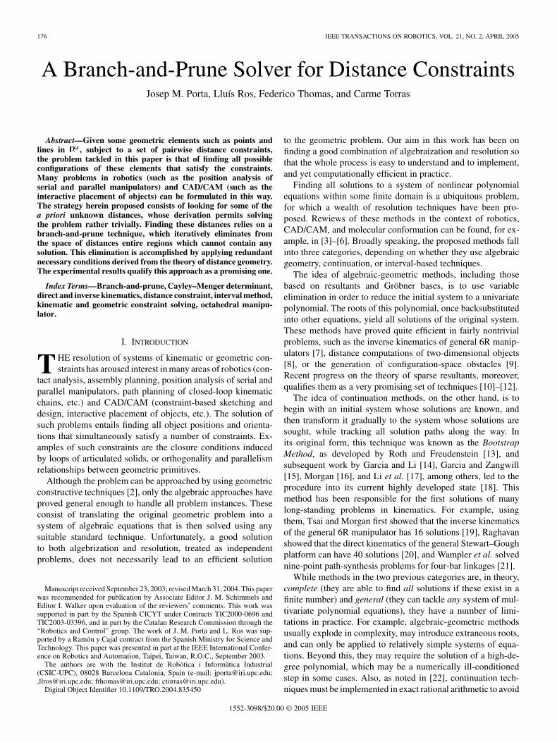
Fig. 1. Top: (a) a general 6R linkage and its equivalent bar-and-joint model. (b) A tetrahedral ring. Bottom: (c) a Puma 560 robot with, overlaid, its six binarylinks. (d) Its equivalent bar-and-joint model.
The points are embeddable in , satisfying theprescribed distances between them, if, and only if, all the fol-lowing conditions are met:
R1) all Cayley–Menger determinants of three such pointsare either negative or zero;
R2) all Cayley–Menger determinants of four points areeither positive or zero;
R3) all Cayley-Menger determinants of five and six pointsvanish.
Note that conditions R1, R2, and R3 are indeed necessary as,in accordance with (2), (3), and (4), a Cayley–Menger deter-minant must be negative or zero, positive or zero, or strictlyzero, depending on whether it involves three, four, or more thanfour points, respectively. Actually, Blumenthal proves a slightlystronger version of this theorem, in which it is sufficient tofind an ordering of such that the first four points inthis ordering satisfy conditions R1 and R2, and then only thoseCayley–Menger determinants of five and six points that includethese four points vanish. For the purpose of this paper, though,the previous weaker version will be used, as it provides extraredundant equations that enhance the convergence behavior ofthe presented solver.
III. FROM KINEMATIC AND GEOMETRIC CONSTRAINTS
TO DISTANCE CONSTRAINTS
Many problems of direct and inverse kinematics can be ex-pressed in terms of systems of distance constraints, like thosederived from conditions R1–R3 above. Consider, for example,
the problem of finding all valid configurations of a closed 6Rlinkage, a cycle of six binary links pairwise articulated with rev-olute joints [Fig. 1(a)]. A binary link can be modeled by takingtwo points on each of its two revolute axes and connecting thefour points with rigid bars to form a tetrahedron. Bars meetingat a common point are thought of as articulated through idealball-socket joints. By doing so, a 6R linkage is easily trans-lated into a ring of six tetrahedra, pairwise articulated througha common edge [Fig. 1(b)]. Observe that the valid configura-tions of this ring are in one-to-one correspondence with those ofthe original 6R linkage. Since the ring only involves ball-socketjoints and rigid bars, it can be regarded as a set of points (thejoints) that keep some prescribed distances between them (thebars). Hence, all unknown distances within the ring must ful-fill all conditions R1–R3, above which, when gathered together,they form a polynomial system whose solutions yield the validpostures of the ring.
When the axes of a link are not skew but intersecting, thelink can be modeled by a rigid triangle rather than by a tetrahe-dron, thus using less ball-socket joints and bars. The case of thePUMA 560 robot depicted in Fig. 1(c) illustrates this. As in eachof the links , , , and , the two axes are copunctual, theycan be substituted by a triangle in the equivalent bar-and-jointmodel of Fig. 1(d). The last link is fictitious, but it is drawnhere to emphasize that, in the inverse kinematics of such a robot,the desired position for the robot’s hand is a priori known.
This process can be generalized to larger classes of mecha-nisms. When multiple loops are present, for example, some ofthe links will not be binary, but will necessarily involve three
PORTA et al.: A BRANCH-AND-PRUNE SOLVER FOR DISTANCE CONSTRAINTS 179
Fig. 2. Sarrus’s mechanism. Since the axes of the three revolute pairs in eachleg are parallel, body B can only translate with respect to B and, hence, thisdevice can be used to implement a prismatic pair using revolute joints alone.
or more joint axes. In general, a link with revolute axes iseasily modeled by taking two points on each axis and placingall possible bars between the selected points to make thewhole compound rigid. On the other hand, if a prismatic pair ispresent, one can always substitute it with Sarrus’s equivalentmechanism (Fig. 2), made up with revolute joints alone, andapply the previous transformations to its links. In any case, ifonly revolute and prismatic pairs are present, a reduction to anequivalent bar-and-joint model is always possible, for which asystem of coordinate-free equations giving its valid configura-tions can be set up by using conditions R1–R3.
An interesting remark here is that one may be able to detectthat a closed-form solution for the mechanism is available, bysimply examining which unknowns are present in each of theequations derived from condition R3, without requiring any al-gebraic manipulation of them. For example, it can be seen that,for the PUMA 560, a sequence of ten Cayley–Menger equationsof five points can be selected among the points , , , , , , ,and of Fig. 1(d), such that every equation in the sequence con-tains one more variable than the preceding one. Being in echelonform and quadratic in all unknowns, this subsystem is solvablein closed form, and already determines the ten unknown dis-tances among these points, the ten missing “bars” in Fig. 1(d).
Many geometric constraints can also be expressed in a coor-dinate-free form in terms of distances, by using Cayley–Mengerdeterminants. To give some examples, we here derive three suchconstraints: collinear points, orthogonal segments, and point-line distance.
• Three points , , and are collinear if, and only if,. This follows from (2), since the area
of the triangle defined by three collinear points is null.• Two adjacent segments and are orthogonal if,
and only if, . Thisis a rewriting of Pythagoras’ theorem by using (1).
• Finally, the distance between a point and a linepassing through and satisfies the equation
(5)
which follows from (2) and the fact that, in this case,.
Section V will exemplify how some kinematic and geometricconstraint-solving problems can be formulated and solved onthe basis of the distance constraints introduced above.
IV. THE ALGORITHM
We now present an algorithm able to solve systems of multi-linear constraints. Since both Cayley–Menger determinants andidentity relations are multilinear, this algorithm canbe readily used to solve systems of distance constraints, likethose derived in the previous section for kinematic or geometricconstraint-solving problems. Specifically, for a system
(6)
where , , andeach function or is multilinear in the unknowns(the unknown distances , in our case), the algorithm is ableto isolate all solutions that lie in a prespecified rectangular box
of . is defined as the Cartesian product, where denotes the closed real interval in
which the solution values for must be sought.
A. Branch-and-Prune Scheme
Generally speaking, the algorithm isolates the solutions by it-erating two operations, box reduction and box bisection, usingthe following branch-and-prune scheme. Using box reduction,portions of containing no solution are cut off by narrowingsome of its defining intervals. This process is iterated until ei-ther the box is reduced to an empty set, in which case it containsno solution, or the box is “sufficiently” small, in which case it isconsidered a solution box, or the box cannot be “significantly”reduced, in which case it is split into two subboxes via box bi-section. If the latter occurs, the whole process is repeated forthe newly created subboxes, and for the subboxes recursivelycreated thereafter, until one ends up with a collection of boxeswhose size is under a specified size threshold, as explained indetail below.
If there is only a finite number of solution points in , thisalgorithm returns a collection of small boxes containing themall. If, contrarily, the solution space is an algebraic variety ofdimension one or higher, the algorithm returns a collection ofsmall boxes discretizing the portions of this variety contained in
. In all cases, the algorithm is complete, in the sense that everysolution point will be contained in one of the returned boxes.
Let us now follow the box reduction and bisection operationsin detail, to later see how they fit into the solver’s algorithm.
B. Box Reduction and Box Bisection
The box-reduction operation is based on the followinglemma, which is a direct consequence of [33, Th. 1].
The point , where is a scalar mul-tilinear function and is a point lying in
, is contained in the convexhull of the points
.
180 IEEE TRANSACTIONS ON ROBOTICS, VOL. 21, NO. 2, APRIL 2005
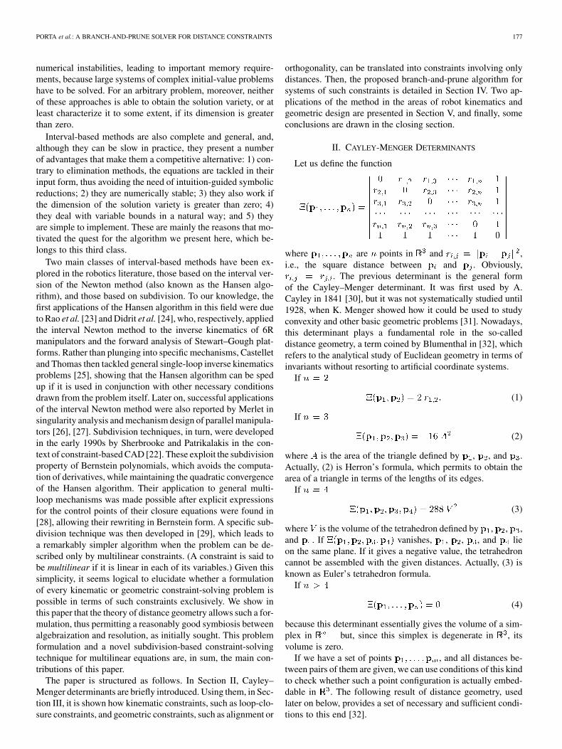
Fig. 3. Segment-trapezoid clipping. Top: in this two-variable case, the graphof f(x ; x ) corresponding to points in B necessarily lies inside the showntetrahedron H. The vertices of H are obtained by evaluating f in the cornersof B. Bottom: from the initial range for a variable, we can prune all points forwhich its trapezoid does not intersect the f(x ; x ) = 0 line.
In other words, the graph of corresponding to a boxnecessarily lies inside the convex hull of the points of theform , where is a corner of .
This result can be readily used to refine an initial bound ofthe solution space of the system (6). For the sake of clarity, weexplain how this is done when (6) consists of just one equation intwo variables, and show at the end how the same process directlyapplies to the general case.
Assume that we want to find all solutions of a multilinearequation , for in the box
(Fig. 3). Since must lie within theconvex hull of the points
of , we can compute and intersect it with theplane to obtain a polygon whose smallest enclosingbox gives a better bound for the solutions. Since the explicitcomputation of and its intersection with are in-efficient operations when depends on a high number of vari-ables, we will adopt the following variation of this technique.We simply project the hull onto each coordinate plane, as de-picted in Fig. 3 (top), and intersect each of the resulting trape-zoids with the line, as shown in Fig. 3 (bottom).Clearly, from the initial range of a variable, we can prune thosepoints for which the trapezoid does not intersect the
line. Thus, these segment-trapezoid clippings usually reduce theranges of some variables, giving a smaller box that still boundsthe root locations (see the black rectangle in Fig. 3). The exper-iments show that although this strategy produces less pruningthan the convex hull-plane clipping, its results are advantageousdue to the lower cost of its operations.
Note that exactly the same pruning strategy can be appliedfor a multilinear equation in variables, with , becausethe convex hull of the (then) involved points will also yielda trapezoidal polygon when projected to a plane defined by the
and axes, for . Also, if instead of an equa-tion, we have an inequation , we proceed similarly bypruning all values of a variable range for which its trapezoid en-tirely lies in the half-plane. Finally, if we have morethan one constraint in the system, the process can be clearly iter-ated for all constraints by applying the pruning process of eachconstraint onto the box produced by the pruning process of thepreceding one.
The previous box-reduction procedure is repeatedly appliedon the same box until one of the following conditions is met.
• The box gets empty. This happens when we are treating aninequation , and the trapezoid for some variablein is entirely in the half-plane, or whenwe are treating an equation , and a trapezoiddoes not intersect the line. In any case, a wholevariable range is pruned, and we can stop the explorationin the search space the current box delimits.
• The reduction of the box volume between two consecutiveiterations is below a given threshold . At this point, asthe box cannot be significantly reduced, it is split into twosubboxes via box bisection. This operation simply dividesthe longest variable range of the box into two halves, inorder to keep the shape of the resulting subboxes as cubicas possible. Box reduction and bisection are then recur-sively applied to the newly created subboxes.
• The longest side of the box is under a specified threshold. Here, the box is considered a “solution box” since, if
is sufficiently small, either this box contains a solution oris very close to one. Hence, it is added to the final list ofboxes to be returned by the algorithm.
C. Pseudocode
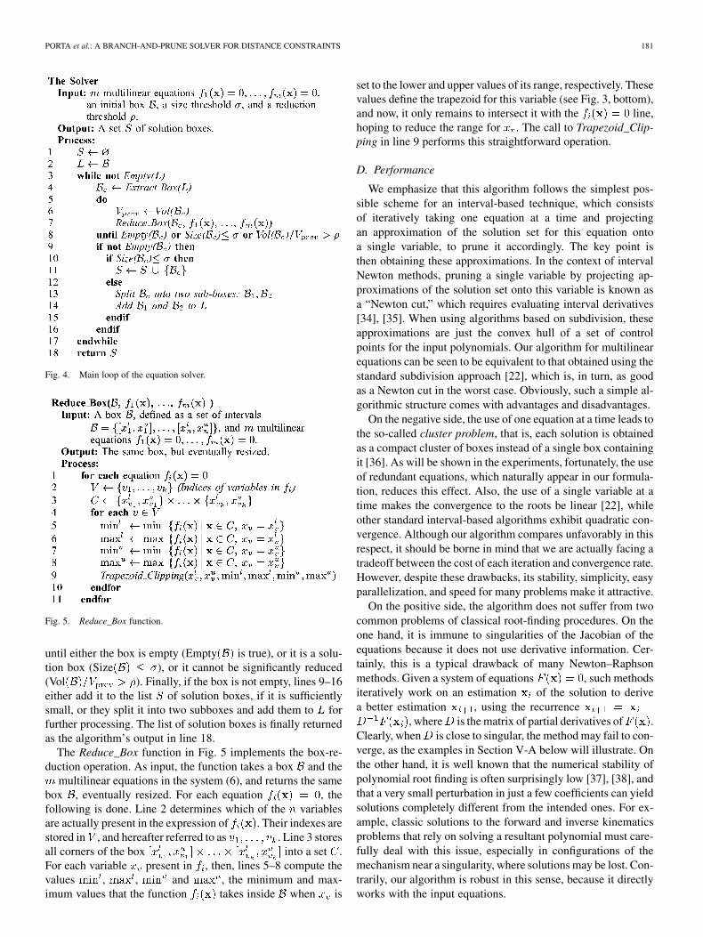
For the sake of conciseness, the given pseudocode only man-ages equations. Its extension to also deal with inequations isstraightforward, if we take into account all comments above.The main loop, as schematized in Fig. 4, uses the followingconventions. The arrow “ ” is the assignment operator. TheBoolean expression Empty is evaluated to true when any ofthe defining intervals of is empty. The function Extract_Boxreturns (and removes) one box from its list argument. The ex-pressions Vol and Size denote the volume of and thelength of the longest side of .
Initially, two lists are set up (lines 1 and 2), a list of “boxesto be processed,” and a list of “solution boxes.” is initializedto contain , and to an empty list. A while loop is then exe-cuted until gets empty (lines 3–17), by iterating the followingsteps. Line 4 extracts the first box in . Lines 5–8 repeatedly re-duce this box as much as possible, via the Reduce_Box function,
PORTA et al.: A BRANCH-AND-PRUNE SOLVER FOR DISTANCE CONSTRAINTS 181
Fig. 4. Main loop of the equation solver.
Fig. 5. Reduce_Box function.
until either the box is empty (Empty is true), or it is a solu-tion box (Size ), or it cannot be significantly reduced(Vol ). Finally, if the box is not empty, lines 9–16either add it to the list of solution boxes, if it is sufficientlysmall, or they split it into two subboxes and add them to forfurther processing. The list of solution boxes is finally returnedas the algorithm’s output in line 18.
The Reduce_Box function in Fig. 5 implements the box-re-duction operation. As input, the function takes a box and the
multilinear equations in the system (6), and returns the samebox , eventually resized. For each equation , thefollowing is done. Line 2 determines which of the variablesare actually present in the expression of . Their indexes arestored in , and hereafter referred to as . Line 3 storesall corners of the box into a set .For each variable present in , then, lines 5–8 compute thevalues , , and , the minimum and max-imum values that the function takes inside when is
set to the lower and upper values of its range, respectively. Thesevalues define the trapezoid for this variable (see Fig. 3, bottom),and now, it only remains to intersect it with the line,hoping to reduce the range for . The call to Trapezoid_Clip-ping in line 9 performs this straightforward operation.
D. Performance
We emphasize that this algorithm follows the simplest pos-sible scheme for an interval-based technique, which consistsof iteratively taking one equation at a time and projectingan approximation of the solution set for this equation ontoa single variable, to prune it accordingly. The key point isthen obtaining these approximations. In the context of intervalNewton methods, pruning a single variable by projecting ap-proximations of the solution set onto this variable is known asa “Newton cut,” which requires evaluating interval derivatives[34], [35]. When using algorithms based on subdivision, theseapproximations are just the convex hull of a set of controlpoints for the input polynomials. Our algorithm for multilinearequations can be seen to be equivalent to that obtained using thestandard subdivision approach [22], which is, in turn, as goodas a Newton cut in the worst case. Obviously, such a simple al-gorithmic structure comes with advantages and disadvantages.
On the negative side, the use of one equation at a time leads tothe so-called cluster problem, that is, each solution is obtainedas a compact cluster of boxes instead of a single box containingit [36]. As will be shown in the experiments, fortunately, the useof redundant equations, which naturally appear in our formula-tion, reduces this effect. Also, the use of a single variable at atime makes the convergence to the roots be linear [22], whileother standard interval-based algorithms exhibit quadratic con-vergence. Although our algorithm compares unfavorably in thisrespect, it should be borne in mind that we are actually facing atradeoff between the cost of each iteration and convergence rate.However, despite these drawbacks, its stability, simplicity, easyparallelization, and speed for many problems make it attractive.
On the positive side, the algorithm does not suffer from twocommon problems of classical root-finding procedures. On theone hand, it is immune to singularities of the Jacobian of theequations because it does not use derivative information. Cer-tainly, this is a typical drawback of many Newton–Raphsonmethods. Given a system of equations , such methodsiteratively work on an estimation of the solution to derivea better estimation , using the recurrence
, where is the matrix of partial derivatives of .Clearly, when is close to singular, the method may fail to con-verge, as the examples in Section V-A below will illustrate. Onthe other hand, it is well known that the numerical stability ofpolynomial root finding is often surprisingly low [37], [38], andthat a very small perturbation in just a few coefficients can yieldsolutions completely different from the intended ones. For ex-ample, classic solutions to the forward and inverse kinematicsproblems that rely on solving a resultant polynomial must care-fully deal with this issue, especially in configurations of themechanism near a singularity, where solutions may be lost. Con-trarily, our algorithm is robust in this sense, because it directlyworks with the input equations.
182 IEEE TRANSACTIONS ON ROBOTICS, VOL. 21, NO. 2, APRIL 2005
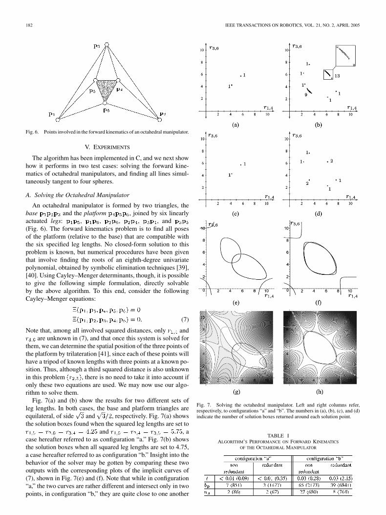
Fig. 6. Points involved in the forward kinematics of an octahedral manipulator.
V. EXPERIMENTS
The algorithm has been implemented in C, and we next showhow it performs in two test cases: solving the forward kine-matics of octahedral manipulators, and finding all lines simul-taneously tangent to four spheres.
A. Solving the Octahedral Manipulator
An octahedral manipulator is formed by two triangles, thebase and the platform , joined by six linearlyactuated legs: , , , , , and(Fig. 6). The forward kinematics problem is to find all posesof the platform (relative to the base) that are compatible withthe six specified leg lengths. No closed-form solution to thisproblem is known, but numerical procedures have been giventhat involve finding the roots of an eighth-degree univariatepolynomial, obtained by symbolic elimination techniques [39],[40]. Using Cayley–Menger determinants, though, it is possibleto give the following simple formulation, directly solvableby the above algorithm. To this end, consider the followingCayley–Menger equations:
(7)
Note that, among all involved squared distances, only andare unknown in (7), and that once this system is solved for
them, we can determine the spatial position of the three points ofthe platform by trilateration [41], since each of these points willhave a tripod of known lengths with three points at a known po-sition. Thus, although a third squared distance is also unknownin this problem , there is no need to take it into account ifonly these two equations are used. We may now use our algo-rithm to solve them.
Fig. 7(a) and (b) show the results for two different sets ofleg lengths. In both cases, the base and platform triangles areequilateral, of side and , respectively. Fig. 7(a) showsthe solution boxes found when the squared leg lengths are set to
and , acase hereafter referred to as configuration “a.” Fig. 7(b) showsthe solution boxes when all squared leg lengths are set to 4.75,a case hereafter referred to as configuration “b.” Insight into thebehavior of the solver may be gotten by comparing these twooutputs with the corresponding plots of the implicit curves of(7), shown in Fig. 7(e) and (f). Note that while in configuration“a,” the two curves are rather different and intersect only in twopoints, in configuration “b,” they are quite close to one another
Fig. 7. Solving the octahedral manipulator. Left and right columns refer,respectively, to configurations “a” and “b”. The numbers in (a), (b), (c), and (d)indicate the number of solution boxes returned around each solution point.
TABLE IALGORITHM’S PERFORMANCE ON FORWARD KINEMATICS
OF THE OCTAHEDRAL MANIPULATOR
PORTA et al.: A BRANCH-AND-PRUNE SOLVER FOR DISTANCE CONSTRAINTS 183
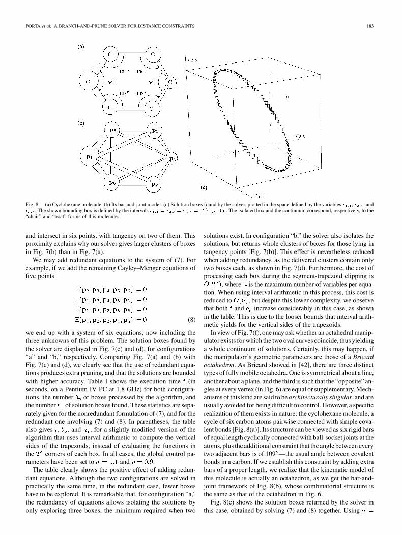
Fig. 8. (a) Cyclohexane molecule. (b) Its bar-and-joint model. (c) Solution boxes found by the solver, plotted in the space defined by the variables r , r , andr . The shown bounding box is defined by the intervals r = r = r = [2:75; 3:95]. The isolated box and the continuum correspond, respectively, to the“chair” and “boat” forms of this molecule.
and intersect in six points, with tangency on two of them. Thisproximity explains why our solver gives larger clusters of boxesin Fig. 7(b) than in Fig. 7(a).
We may add redundant equations to the system of (7). Forexample, if we add the remaining Cayley–Menger equations offive points
(8)
we end up with a system of six equations, now including thethree unknowns of this problem. The solution boxes found bythe solver are displayed in Fig. 7(c) and (d), for configurations“a” and “b,” respectively. Comparing Fig. 7(a) and (b) withFig. 7(c) and (d), we clearly see that the use of redundant equa-tions produces extra pruning, and that the solutions are boundedwith higher accuracy. Table I shows the execution time (inseconds, on a Pentium IV PC at 1.8 GHz) for both configura-tions, the number of boxes processed by the algorithm, andthe number of solution boxes found. These statistics are sepa-rately given for the nonredundant formulation of (7), and for theredundant one involving (7) and (8). In parentheses, the tablealso gives , , and , for a slightly modified version of thealgorithm that uses interval arithmetic to compute the verticalsides of the trapezoids, instead of evaluating the functions inthe corners of each box. In all cases, the global control pa-rameters have been set to and .
The table clearly shows the positive effect of adding redun-dant equations. Although the two configurations are solved inpractically the same time, in the redundant case, fewer boxeshave to be explored. It is remarkable that, for configuration “a,”the redundancy of equations allows isolating the solutions byonly exploring three boxes, the minimum required when two
solutions exist. In configuration “b,” the solver also isolates thesolutions, but returns whole clusters of boxes for those lying intangency points [Fig. 7(b)]. This effect is nevertheless reducedwhen adding redundancy, as the delivered clusters contain onlytwo boxes each, as shown in Fig. 7(d). Furthermore, the cost ofprocessing each box during the segment-trapezoid clipping is
, where is the maximum number of variables per equa-tion. When using interval arithmetic in this process, this cost isreduced to , but despite this lower complexity, we observethat both and increase considerably in this case, as shownin the table. This is due to the looser bounds that interval arith-metic yields for the vertical sides of the trapezoids.
In view of Fig. 7(f), one may ask whether an octahedral manip-ulator exists for which the two oval curves coincide, thus yieldinga whole continuum of solutions. Certainly, this may happen, ifthe manipulator’s geometric parameters are those of a Bricardoctahedron. As Bricard showed in [42], there are three distincttypes of fully mobile octahedra. One is symmetrical about a line,another about a plane, and the third is such that the “opposite” an-gles at every vertex (in Fig. 6) are equal or supplementary. Mech-anisms of this kind are said to be architecturally singular, and areusually avoided for being difficult to control. However, a specificrealization of them exists in nature: the cyclohexane molecule, acycle of six carbon atoms pairwise connected with simple cova-lent bonds [Fig. 8(a)]. Its structure can be viewed as six rigid barsof equal length cyclically connected with ball-socket joints at theatoms, plus the additional constraint that the angle between everytwo adjacent bars is of 109 —the usual angle between covalentbonds in a carbon. If we establish this constraint by adding extrabars of a proper length, we realize that the kinematic model ofthis molecule is actually an octahedron, as we get the bar-and-joint framework of Fig. 8(b), whose combinatorial structure isthe same as that of the octahedron in Fig. 6.
Fig. 8(c) shows the solution boxes returned by the solver inthis case, obtained by solving (7) and (8) together. Using
184 IEEE TRANSACTIONS ON ROBOTICS, VOL. 21, NO. 2, APRIL 2005
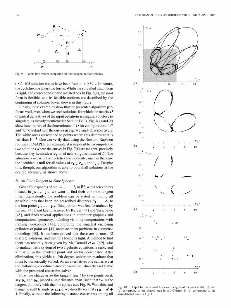
Fig. 9. Points involved in computing all lines tangent to four spheres.
, 105 solution boxes have been found, in 0.39 s. In nature,the cyclohexane takes two forms. While the so-called chair formis rigid, and corresponds to the isolated box in Fig. 8(c), the boatform is flexible, and its feasible motions are described by thecontinuum of solution boxes shown in this figure.
Finally, these examples show that the presented algorithm per-forms well, even when we seek solutions for which the matrixof partial derivatives of the input equations is singular (or close tosingular), as already mentioned in Section IV-D. Fig. 7(g) and (h)show isocontours of the determinant of for configurations “a”and “b,” overlaid with the curves in Fig. 7(e) and (f), respectively.The white areas correspond to points where this determinant isless than . One can verify that, using the Newton–Raphsonroutines of MAPLE, for example, it is impossible to compute thetwo solutions where the curves in Fig. 7(f) are tangent, preciselybecause they lie inside a region of near-singularitiness of . Thesituation is worse in the cyclohexane molecule, since in that casethe Jacobian is null for all values of , , and . Despitethis, though, our algorithm is able to bound all solutions at thedesired accuracy, as shown above.
B. All Lines Tangent to Four Spheres
Given four spheres of radii in , with their centerslocated in , we want to find their common tangentlines. Equivalently, the problem can be stated as finding allpossible lines that keep the prescribed distances tothe four points . This problem was first formulated byLarman [43], and later discussed by Karger [44] and Verschelde[45], and finds several applications in computer graphics andcomputational geometry, including visibility computations withmoving viewpoints [46], computing the smallest enclosingcylinders of point sets [47] and placement problems in geometricmodeling [48]. It has been proved that there are at most 12discrete solutions, and that this bound is tight. A method to findthem has recently been given by MacDonald et al. [49], whoformulate it as a system of two algebraic equations, a cubic anda quartic, in the involved point and vector coordinates. Afterelimination, this yields a 12th-degree univariate resultant thatmust be numerically solved. As an alternative, one can arrive atthe following coordinate-free formulation, directly tackleablewith the presented constraint solver.
First, we characterize the tangent line by two points on it,say and , placed a unit distance apart, such that is thetangent point of with the first sphere (see Fig. 9). With this, andusing the right triangle , we directly see that
. Finally, we state the following distance constraints among all
Fig. 10. Output for the second test case. Lengths of the axes in (b), (c), and(d) correspond to the shaded area in (a). Clusters in (d) correspond to thesame-labeled ones in Fig. 11.
PORTA et al.: A BRANCH-AND-PRUNE SOLVER FOR DISTANCE CONSTRAINTS 185
Fig. 11. Top: clusters of solution boxes found in the second test case. The shown bounding box is defined by the intervals r = r = r = [2:5; 8:8].Bottom: the corresponding 12 lines that keep the specified distances to the given four red points. Each configuration corresponds to the same numbered cluster inthe plot above.
points in , defining a redundant system of tenequations in six unknowns.
C1) Three constraints of the form of (5) to force that thedistance from each of , , to be , , and
, respectively.C2) The two Cayley–Menger equations of five points
, and, each involving three unknowns.
C3) The remaining four Cayley–Menger equations of fivepoints of , three involving four unknowns, and oneinvolving six unknowns.
C4) The unique Cayley–Menger equation of the six pointsin , with six unknowns.
One can now use the solver to treat them all together, but it is il-lustrative to successively apply it to larger subsets of these equa-
tions instead, and see the outputs. Let us study the case where allintercenter distances are , and all radii are 1.45, for which 12solutions exist [49]. If we start by setting and we justconsider the five constraints in C1 and C2, we obtain the 1-Dcontinuum of solutions depicted in Fig. 10(a). The continuumdisappears when we solve C1, C2, and C3 together, as seen inFig. 10(b), giving rise to very large clusters of solution boxes.These can be further reduced if the last constraint C4 is takeninto account, to get the box clusters in Fig. 10(c). At this point,we have exhausted all possible distance constraints between theselected points, and we cannot further reduce the clusters, un-less we ask a higher accuracy from the solver. If we do this, bysetting , we get the small clusters in Fig. 10(d), eachcorresponding to one of the 12 solutions of the problem. Actu-ally, the two pairs of clusters 2–3 and 7–8 appear overlaid, but
186 IEEE TRANSACTIONS ON ROBOTICS, VOL. 21, NO. 2, APRIL 2005
TABLE IIALGORITHM’S PERFORMANCE ON THE “TANGENTS TO
FOUR SPHERES” PROBLEM
they can be seen separated if we plot them on the 3-D spacedefined by , , and . This plot, together with the lineconfiguration corresponding to each cluster, is shown in Fig. 11.
Table II gives the values of , , and for the last two ex-periments. The and columns correspond,respectively, to the computation of Fig. 10(c) and (d). Both ex-periments have been done with . We note that the timeto compute the solutions does not increase substantially, despitethe fact that has been decreased by one order of magnitude inthe second experiment. Furthermore, although a higher numberof boxes is processed for , the final number of solu-tion boxes remains practically the same as for . This isnot casual. One can see that, from a certain point, after askinghigher and higher accuracies from the solver, the number ofboxes around each solution point will practically remain con-stant. The avoidance of this phenomenon, also associated withthe cluster problem observed in [36], constitutes part of our cur-rent research.
VI. CONCLUSIONS
We have presented a general solver for systems of kinematicand geometric constraints. Target applications are those where asystem of constraints on the relative positions of a set of objectsmust be solved, such as those arising in the position analysisof serial and parallel robots, the contact analysis of polyhedralmodels, or the automatic generation of constraint-specified de-signs or assemblies.
A special emphasis has been put on finding a good combi-nation of algebraization and resolution techniques. To this end,the use of standard coordinate-free constraints derived from thetheory of distance geometry, combined with a novel branch-and-prune technique to solve them, has proved efficient, yielding asolver that is conceptually simple and easy to implement. Thesolver is also complete, in the sense that it loses no solutions, andis able to discretize entire continua of solutions if they exist.
According to our experiments, the addition of redundant con-straints speeds up, in general, the resolution process, and re-duces the number of final boxes delivered. Although not illus-trated by the presented examples, the addition of redundant vari-ables, on the contrary, usually introduces a tradeoff between thenumber of final boxes and execution times. As the number ofredundant variables is increased, the solver needs longer exe-cution times, but, in return, it obtains a lower number of finalboxes.
The algorithm as it stands leaves many choices open, as isusually the case in constraint-based search (variable ordering,constraint selection, redundacy dosage, etc.). This offers a rangeof possibilities to speed up the resolution process, which wewill tackle in future research by devising good heuristics for thechoice points above.
REFERENCES
[1] J. M. Porta, L. Ros, F. Thomas, and C. Torras, “A branch-and-prunealgorithm for solving systems of distance constraints,” in IEEE Int. Conf.Robot. Autom., vol. 1, Taipei, Taiwan, R.O.C., Sep. 2003, pp. 342–348.
[2] I. Fudos and C. Hoffmann, “A graph-constructive approach to solvingsystems of geometric constraints,” ACM Trans. Graphics, vol. 16, no. 2,pp. 179–216, 1997.
[3] J. Nielsen and B. Roth, “Formulation and solution for the direct andinverse kinematics problems for mechanisms and mechatronic systems,”in Proc. NATO Adv. Study Inst. Computat. Methods Mechanisms, vol. I,J. Angeles and E. Zakhariev, Eds., Jun. 1997, pp. 233–252.
[4] , “On the kinematic analysis of robotic mechanisms,” Int. J. Robot.Res., vol. 18, no. 12, pp. 1147–1160, 1999.
[5] C. H. Hoffmann and B. Yuan, “On spatial constraints solving ap-proaches,” in Automated Deduction in Geometry: Third InternationalWorkshop, ser. Lecture Notes in Computer Science. New York:Springer, 2000, vol. 2061.
[6] I. Z. Emiris and B. Mourrain, “Computer algebra methods for studyingand computing molecular conformations,” Algorithmica, no. 25, pp.372–402, 1999.
[7] D. Manocha and J. Canny, “Efficient inverse kinematics for general 6rmanipulators,” IEEE Trans. Robot. Autom., vol. 10, pp. 648–657, Jun.1994.
[8] K. Sridharan, “Computing two penetration measures for curved 2d ob-jects,” Inf. Process. Lett., vol. 72, pp. 143–148, 1999.
[9] C. Bajaj and M.-S. Kim, “Generation of configuration space obstacles:Moving algebraic surfaces,” Int. J. Robot. Res., vol. 9, no. 1, pp. 92–112,1990.
[10] D. Kapur and T. Saxena, “Sparsity considerations in Dixon resultants,”in Proc. Annu. ACM Symp. Theory of Computing, 1996, pp. 184–191.
[11] I. Emiris and J. Canny, “Efficient incremental algorithms for the sparseresultant and the mixed volume,” J. Symbolic Comput., vol. 20, no. 2,pp. 117–149, 1995.
[12] J. Canny and I. Emiris, “A subdivision-based algorithm for the sparseresultant,” J. ACM, vol. 47, no. 3, pp. 417–451, 2000.
[13] B. Roth and F. Freudenstein, “Synthesis of path-generating mechanismsby numerical methods,” ASME J. Eng. Ind., vol. 85, pp. 298–307, 1963.
[14] C. B. Garcia and T. Y. Li, “On the number of solutions to polynomialsystems of equations,” SIAM J. Numer. Anal., vol. 17, pp. 540–546, 1980.
[15] C. B. Garcia and W. I. Zangwill, Pathways to Solutions, Fixed Points,and Equilibria. Upper Saddle River, NJ: Prentice-Hall, 1981.
[16] A. P. Morgan, “A homotopy for solving polynomial systems,” Appl.Math. Computat., vol. 18, pp. 87–92, 1986.
[17] T. Y. Li, T. Sauer, and J. A. York, “The cheater’s homotopy: An efficientprocedure for solving systems of polynomial equations,” SIAM J. Numer.Anal., vol. 18, no. 2, pp. 173–177, 1988.
[18] C. Wampler, A. Morgan, and A. Sommese, “Numerical continuationmethods for solving polynomial systems arising in kinematics,” ASMEJ. Mech. Design, vol. 112, pp. 59–68, 1990.
[19] L.-W. Tsai and A. Morgan, “Solving the kinematics of the most generalsix- and five-degree-of-freedom manipulators by continuation methods,”ASME J. Mechan., Trans., Autom. Design, vol. 107, pp. 189–200, 1985.
[20] M. Raghavan, “The Stewart platform of general geometry has 40 con-figurations,” ASME J. Mech. Design, vol. 115, pp. 277–282, 1993.
[21] C. Wampler, A. Morgan, and A. Sommese, “Complete solution of thenine-point path synthesis problem for four-bar linkages,” J. Mech. De-sign, vol. 114, pp. 153–159, 1992.
[22] E. Sherbrooke and N. Patrikalakis, “Computation of the solutions ofnonlinear polynomial systems,” Comput. Aided Geom. Design, vol. 10,no. 5, pp. 379–405, 1993.
[23] R. S. Rao, A. Asaithambi, and S. K. Agrawal, “Inverse kinematic so-lution of robot manipulators using interval analysis,” ASME J. Mech.Design, vol. 120, pp. 147–150, 1998.
[24] O. Didrit, M. Petitot, and E. Walter, “Guaranteed solution of direct kine-matic problems for general configurations of parallel manipulators,”IEEE Trans. Robot. Autom., vol. 14, pp. 259–266, Apr. 1998.
[25] A. Castellet and F. Thomas, “An algorithm for the solution of inversekinematics problems based on an interval method,” in Advances in RobotKinematics, M. Husty and J. Lenarcic, Eds. Norwell, MA: Kluwer,1998, pp. 393–403.
[26] J.-P. Merlet, “A formal numerical approach to determine the presenceof singularity within the workspace of a parallel robot,” in Proc. 2ndWorkshop Computat. Kinematics, Seoul, South Korea, May 2001, pp.167–176.
PORTA et al.: A BRANCH-AND-PRUNE SOLVER FOR DISTANCE CONSTRAINTS 187
[27] , “An improved design algorithm based on interval analysis for par-allel manipulator with specified workspace,” in Proc. IEEE Int. Conf.Robot. Autom., vol. 2, Seoul, South Korea, May 2001, pp. 1289–1294.
[28] C. Bombín, L. Ros, and F. Thomas, “A concise Bézier clipping tech-nique for solving inverse kinematics problems,” in Advances in RobotKinematics, J. Lenarcic and M. Stanisic, Eds. Norwell, MA: Kluwer,2000, pp. 53–61.
[29] J. M. Porta, L. Ros, F. Thomas, and C. Torras, “Solving multi-looplinkages by iterating 2d clippings,” in Advances in Robot Kinematics,F. Thomas and J. Lenarcic, Eds. Norwell, MA: Kluwer, 2002, pp.255–264.
[30] A. Cayley, “A theorem in the geometry of position,” Cambridge Math.J., vol. II, pp. 267–271, 1841.
[31] K. Menger, “New foundation for Euclidean geometry,” Amer. J. Math.,no. 53, pp. 721–745, 1931.
[32] L. Blumenthal, Theory and Applications of Distance Geometry. Ox-ford, U.K.: Oxford Univ. Press, 1953.
[33] A. Rikun, “A convex envelope formula for multilinear functions,” J.Global Optim., vol. 10, pp. 425–437, 1997.
[34] P. V. Hentenryck, D. McAllester, and D. Kapur, “Three cuts for accel-erating interval propagation,” MIT, Artif. Intell. Lab., Cambridge, MA,Tech. Rep., 1995.
[35] , “Solving polynomial systems using a branch and prune approach,”SIAM J. Numer. Anal., vol. 34, no. 2, pp. 797–827, 1997.
[36] A. Morgan and V. Shapiro, “Box-bisection for solving second-degreesystems and the problem of clustering,” ACM Trans. Math. Software,vol. 13, no. 2, pp. 152–167, 1987.
[37] A. Ralston and P. Rabinowitz, A First Course in Numerical Analysis,2nd ed. New York: McGraw-Hill, 1978.
[38] D. Kahaner, C. Moler, and S. Nash, Numerical Methods and Soft-ware. Englewood Cliffs, NJ: Prentice-Hall, 1989.
[39] M. Griffis and J. Duffy, “A forward displacement analysis of a class ofStewart platforms,” J. Robot. Syst., vol. 6, pp. 703–720, 1989.
[40] P. Nanua, K. Waldron, and V. Murthy, “Direct kinematic solution of aStewart platform,” IEEE Trans. Robot. Autom., vol. 6, pp. 438–444, Aug.1990.
[41] F. Thomas, E. Ottaviano, L. Ros, and M. Ceccarelli, “Coordi-nate-free formulation of a 3-2-1 wire-based tracking device based onCayley–Menger determinants,” in IEEE Int. Conf. Robot. Autom., vol.1, Taipei, Taiwan, R.O.C., May 2003, pp. 355–361.
[42] R. Bricard, “Mémoire sur la théorie de l’octaèdre articulé” (in French),J. Math. Pures et Appliquées, no. 3, pp. 113–148, 1897.
[43] D. Larman, “Problem posed in the problem session of the DIMACSworkshop on arrangements,” Rutgers Univ., New Brunswick, NJ, 1990.
[44] A. Karger, “Classical geometry and computers,” J. Geom. Graphics, vol.2, no. 1, pp. 7–15, 1998.
[45] J. Verschelde, “Polynomial homotopies for dense, sparse and determi-nantal systems,” Dept. Math., Michigan State Univ., East Lansing, MI,Tech. Rep. 1999-041, 1999.
[46] O. Devillers, V. Dujmovic, H. Everett, X. Goaoc, S. Lazard, H.-S. Na,and S. Petitjean, “The expected number of 3D visibility events is linear,”INRIA, Rennes, France, Tech. Rep. 4671, Dec. 2002.
[47] P. Agarwal, B. Aronov, and M. Sharir, “Line transversals of balls andsmallest enclosing cylinders in three dimensions,” Discr. Computat.Geom., no. 21, pp. 373–388, 1999.
[48] C. Durand, “Symbolic and numerical techniques for constraint solving,”Ph.D. dissertation, Purdue Univ., West Lafayette, IN, 1998.
[49] I. Macdonald, J. Pach, and T. Theobald, “Common tangents to four unitballs in R ,” Discr. Computat. Geom., vol. 26, no. 1, pp. 1–17, 2001.
Josep M. Porta received the Engineer degree in com-puter science in 1994 and the Ph.D. degree in artificialintelligence in 2001, both from the Technical Univer-sity of Catalonia, Catalonia, Spain.
He performed research in legged robots, machinelearning, vision-based methods for autonomousrobot localization and computational kinematics.Currently, he holds a Postdoc position at the Institutde Robòtica i Informàtica Industrial, Spanish Scien-tific Research Council, Barcelona, Spain.
Lluís Ros received the mechanical engineering de-gree in 1992, and the Ph.D. degree (with honors) inindustrial engineering in 2000, both from the Tech-nical University of Catalonia, Catalonia, Spain.
From 1993 to 1996 he worked with the Control ofResources Group, Institut de Cibernètica, Barcelona,Spain, involved in the application of constraint logicprogramming to the control of electric and water net-works. Since August 2000, he has been a ResearchScientist with the Institut de Robòtica i InformàticaIndustrial, Spanish Scientific Research Council,
Barcelona, Spain. His research interests include geometry and kinematics, withapplications to robotics, computer graphics, and machine vision.
Federico Thomas received the B.Sc. degree intelecommunications engineering in 1984, and thePh.D. degree (with honors) in computer sciencein 1988, both from the Technical University ofCatalonia, Catalonia, Spain.
Since March 1990, he has been a Research Scien-tist with the Institut de Robòtica i Informàtica Indus-trial, Spanish High Council for Scientific Research,Barcelona, Spain. His research interests are in ge-ometry and kinematics, with applications to robotics,computer graphics, and machine vision.
Carme Torras received the M.Sc. degrees in mathe-matics and computer science from the University ofBarcelona, Barcelona, Spain, and the University ofMassachusetts, Amherst, respectively, and the Ph.D.degree in computer science from the Technical Uni-versity of Catalonia, Catalonia, Spain.
She is currently a Research Professor withthe Spanish Scientific Research Council (CSIC),Barcelona, Spain. She has published four booksand more than 100 papers in the areas of robotkinematics, geometric reasoning, computer vision,
and neurocomputing. She has been local project leader of several Europeanprojects, such as “Planning RObot Motion” (PROMotion), “Robot Controlbased on Neural Network Systems” (CONNY), “Self-organization and Analog-ical Modeling using Subsymbolic Computing” (SUBSYM), and “BehavioralLearning: Sensing and Acting” (B-LEARN).