20 IEEE TRANSACTIONS ON ROBOTICS, VOL. 32,...

20 IEEE TRANSACTIONS ON ROBOTICS, VOL. 32, NO. 1, FEBRUARY 2016

Elastic Stability of Concentric Tube Robots:A Stability Measure and Design Test

Hunter B. Gilbert, Student Member, IEEE, Richard J. Hendrick, Student Member, IEEE, andRobert J. Webster III, Senior Member, IEEE

Abstract—Concentric tube robots are needle-sized manipulatorswhich have been investigated for use in minimally invasive surg-eries. It was noted early in the development of these devices thatelastic energy storage can lead to a rapid snapping motion for de-signs with moderate to high tube curvatures. Substantial progresshas recently been made in the concentric tube robot communityin designing snap-free robots, planning stable paths, and charac-terizing conditions that result in snapping for specific classes ofconcentric tube robots. However, a general measure for determin-ing the stability of a given robot configuration has yet to be pro-posed. In this paper, we use bifurcation and elastic stability theoryto provide such a measure, as well as to produce a test for deter-mining whether a given design is snap-free (i.e., whether snappingcan occur anywhere in the unloaded robot’s workspace). These re-sults are useful in designing, planning motions for, and controllingconcentric tube robots with high curvatures.

Index Terms—Concentric tube robot, continuum robot, medicalrobots and systems.

I. INTRODUCTION

CONCENTRIC tube robots appear to be promising in manykinds of minimally invasive surgical interventions that

require small diameter robots with articulation inside the body.Examples include surgery in the eye [2], heart [3], sinuses [4],lungs [5], prostate [6], brain [7], and other areas. For a review ofconcentric robot development and applications, see [8]. In mostof these applications, higher curvature is generally desirable toenable the robot to turn “tighter corners” inside the human bodyand work dexterously at the surgical site.

However, it was noted early in the development of concen-tric tube robots that unless gradual tube curvatures are usedor minimal overlap of curved tube sections is ensured, tubes

Manuscript received February 6, 2015; revised October 2, 2015; acceptedNovember 5, 2015. Date of publication December 17, 2015; date of currentversion February 3, 2016. This paper was recommended for publication byAssociate Editor Y. Lou and Editor B. J. Nelson upon evaluation of the re-viewers’ comments. This work was supported in part by the National ScienceFoundation (NSF) under CAREER award IIS-1054331 and Graduate ResearchFellowship DGE-0909667, in part by the National Institutes of Health (NIH)under award R01 EB017467, and in part by the global collaborative R&D pro-gram, which was funded by the Ministry of Trade, Industry & Energy (MOTIE,Korea, N0000890). Any opinions, findings, and conclusions or recommenda-tions expressed in this material are those of the authors and do not necessarilyreflect the views of the NSF, NIH, or MOTIE. (H. B. Gilbert and R. J. Hendrickcontributed equally to this work.)

The authors are with the Department of Mechanical Engineering, VanderbiltUniversity, Nashville, TN 37235 USA (e-mail: [email protected];[email protected]; [email protected]).

Some of the results in Sections IV-A, V-A, and Algorithm 1 appeared inpreliminary form in [1].

This paper has supplementary downloadable material available at http://ieeexplore.ieee.org.

Color versions of one or more of the figures in this paper are available onlineat http://ieeexplore.ieee.org.

Digital Object Identifier 10.1109/TRO.2015.2500422

can exhibit elastic instabilities [9] (also previously referred toas “snaps” and “bifurcations”). Elastic instabilities occur dueto torsional elastic energy storage in the tubes that make up aconcentric tube robot. An instability occurs when this energyis rapidly released and the robot “snaps” to a new configura-tion. Unforeseen snapping is clearly not desirable, and could bedangerous in surgical applications.

The snapping problem has been approached from design,modeling, and planning perspectives. With the exception of theearly work in [9], these studies have used the mechanics-basedmodel of concentric tube robots found in [10] and [11]. Forexample, it has recently been shown that tubes can be laser-machined to reduce the ratio of bending to torsional stiffness,which improves stability [12], [13]. However, even using thisapproach, snaps will still occur if high curvatures are employed;therefore, methods for the design and snap prediction will stillbe needed. Another approach is to use nonconstant precurvaturetubes to enhance the elastic stability, as shown by Ha et al. [14].In that study, analytical stability conditions for a two-tube robotwith planar precurvatures are presented and an optimal controlproblem is used to design the tube precurvatures, which resultin a completely stable actuation space. Our study complementstheirs by analyzing the stability of the robots which possessunstable configurations in their actuation space. We also con-sider designs of an arbitrary number of tubes with more generalprecurvature.

It is also possible to plan stable paths for robots that do havethe potential to snap, as shown by Bergeles et al. [7], by examin-ing the relative axial angle between the base of a tube and its tipfor all possible rotations for a given set of tubes. While this workprovides a method to design and use high-curvature robots, thestability condition chosen by the authors was stated as a defini-tion. One of the contributions of our paper is to derive a stabilitycriterion from first principles. Another model-based approach isthat of Xu et al. [15], who sought design parameter bounds forconstant curvature robots to ensure a snap-free unloaded robotworkspace. Xu et al. provided the exact design bounds for a two-tube robot and nonexact, conservative bounds for robots withmore than two tubes. In addition, the solutions in [15] for morethan two tubes only apply to robot configurations where theprecurved portions of tubes are precisely aligned in arc length.

In this paper, we characterize the solution multiplicity andelastic stability of unloaded concentric tube robots with anynumber of tubes, each of which may be preshaped as a generalspace curve. We do this by analyzing the stability propertiespredicted by the accepted model, which has been experimen-tally validated in the literature [10], [11]. We connect concen-tric tube robot stability analysis to the analysis of post-buckled

1552-3098 © 2015 IEEE. Personal use is permitted, but republication/redistribution requires IEEE permission.See http://www.ieee.org/publications standards/publications/rights/index.html for more information.

GILBERT et al.: ELASTIC STABILITY OF CONCENTRIC TUBE ROBOTS: A STABILITY MEASURE AND DESIGN TEST 21

Euler beams from the mechanics literature [16]–[18]. Based onthis analysis, we also propose a measure for relative stability,which can be used to inform real-time controllers, planners, andautomated designers to safely design and operate a robot thatwould otherwise snap. We also show that from the perspectiveof bifurcation theory [19], one can derive an exact, analyticmethod which predicts the stability properties throughout theentire actuation space of a concentric tube robot with constantprecurvature tubes.

II. BEAM BUCKLING ANALOGY

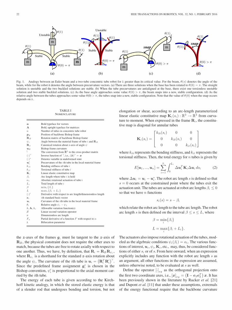
A two tube concentric tube robot and a loaded beam are anal-ogous systems, and both systems exhibit buckling and snapping.To build intuition, we begin by describing these analogous be-haviors. Concentric tube robots are controlled by prescribingrelative translations and rotations at the proximal ends of thetubes. The tubes twist and bend one another along their arclength s. When there are two circularly precurved tubes, thetwist angle between them θ(s) is governed by the same dif-ferential equation as a beam under a dead load, as shown inFig. 1. The configuration of both systems is determined by thenonlinear boundary value problem

f [λ, θ(s)] = θ′′ − λ sin(θ) = 0

θ(0) = θ0

θ′(1) = 0

(1)

where the equations have been normalized to unit length so that0 ≤ s ≤ 1. For both the beam and the concentric tube robot,it is known that increasing the value of the parameter λ canlead to buckling and instability. For the beam, this parameteris controlled by the material properties, the geometry, and themagnitude of the dead load. Likewise, for the robot, λ involvesthe material properties and geometry of the tubes, but the deadload is replaced by the influence of the tube precurvatures.

In the set of solutions to (1), two straight beam configura-tions exist: θ(s) = 0 and θ(s) = π, which represent the beam inpure tension and compression, respectively. Similarly, for con-centric tubes, two torsionless solutions exist in which the tubeprecurvatures are aligned and antialigned, respectively. Just asa beam in tension cannot buckle, a robot configuration withaligned precurvatures is stable. In contrast, when the beam iscompressed [see Fig. 1(a)] or when the concentric tube robothas antialigned precurvatures [see Fig. 1(b)], the configurationswhich are straight for the beam and torsionless for the robot canbuckle if λ exceeds a critical value. Buckling occurs becausethe solution to (1) becomes nonunique when λ is large enough,and two new, energetically favorable solutions arise in a processknown as bifurcation [see Fig. 1(a) and (b)]. The two new so-lutions are stable, and the original solution becomes unstable atthe point of bifurcation.

For many applications of beam theory, like column buckling,the instability of the trivial, straight configuration is all thatis important, but concentric tube robots typically operate farfrom these area and may exhibit instability at other configura-tions and snap across their workspace, as shown in Fig. 1(d).

The equivalent phenomenon for a beam is shown in Fig. 1(c).Consider an active counter-clockwise rotation of θ(0), startingfrom θ(0) = 0. If λ is small enough, we expect that the beamwill pass stably through a straight configuration when θ(0) = π,and the concentric tube robot will pass stably through the con-figuration with antialigned precurvatures. On the other hand,when λ exceeds the critical value, even when θ(0) = π, thebeam will never straighten out and will instead settle into abuckled configuration, and the concentric tube robot will settleinto a high-torsion configuration. Eventually, as θ(0) increasesto some value beyond π, the buckled configuration becomes un-stable, and some of the stored energy is released as each systemsnaps to a new configuration.

In our stability analysis, since we control θ(0) for concentrictube robots, we seek the value of θ(0) at which a concentric tuberobot will snap. In the beam buckling literature, this problem isreferred to as the stability of postbuckled equilibrium states, andimportant results have emerged in this area in recent years [16]–[18]. There has also been recent interest in robotics in the stablequasistatic manipulation of rods [20]. Before applying theseresults to concentric tube robots, we first present the mechanics-based kinematic model.

III. CONCENTRIC TUBE ROBOT KINEMATICS

We provide a self-contained description of the kinematicmodel which is derived from energy. The kinematic model pre-sented here was first derived in [11] and [21]. We present themodel in a concise form suitable for implementation, and discussthe simplification of the multipoint boundary value problem to atwo-point boundary value problem, which was also mentionedin [11]. We choose the angle of twist and the torsional momentas the model states, which results in continuous solutions, evenacross discontinuities caused by precurvature functions or tubeendpoints.

Table I provides a list of variable definitions, and Fig. 2shows the frame definitions for each tube. Each tube has apredefined shape, which is described with a material-attachedcoordinate frame assignment g∗

i (si) = (R∗i ,p

∗i ) : R → SE(3),

where p∗i (si) is the origin of the frame and R∗

i (si) is the orien-tation of the frame. The frame propagates along the tube withits z-axis tangent to the tube centerline and with unit velocity,so that the variable si is the arc length along the ith tube, and0 ≤ si ≤ Li , where Li is the length of the tube. Without loss ofgenerality, the frames g∗

i are chosen as Bishop frames and obeythe differential relationship

∂

∂sig∗

i (si) = g∗i (si) ξ∗

i (si)

for ξ∗i (si) ∈ se(3). In this case, the “hat” denotes the con-

version (·) : R6 → se(3) as defined in [22]. By the preceding

definitions, ξ∗i (si) = [ (v∗)T (u∗

i (si))T ]T , with v∗ = e3 and

u∗i (si) = [u∗

ix(si) u∗iy (si) 0 ]T .

The model assumes that the combined tubes follow a commoncenterline, which we define as another Bishop frame (RB ,pB ).After the conformation of the tubes, we define the resultingmaterial-attached frame of each tube as gi = (Ri ,pi). While


Fig. 1. Analogy between an Euler beam and a two-tube concentric tube robot for λ greater than its critical value. For the beam, θ(s) denotes the angle of thebeam, while for the robot it denotes the angle between precurvature vectors. (a) There are three solutions when the base has been rotated to θ(0) = π . The straightsolution is unstable and the two buckled solutions are stable. (b) When the tube precurvatures are antialigned at the base, there exist one torsionless unstablesolution and two stable buckled solutions. (c) As the base angle approaches some value θ(0) > π , the beam snaps into a new, stable configuration. (d) As therelative angle between the tubes approaches some value θ(0) > π , the tubes snap into a new, stable configuration. Note that the value of θ(0) when the snap occursdepends on λ.

TABLE INOMENCLATURE

a Bold typeface for vectorsA Bold, upright typeface for matricesn Number of tubes in concentric tube robotpB Position of backbone Bishop frameRB Rotation matrix of backbone Bishop frameψi Angle between the material frame of tube i and RB

Rψ Canonical rotation about z-axis of angle ψ

uB Bishop frame curvature· The conversion from R3 to the cross product matrix(·)∨ Inverse function of ·, i.e., (x)∨ = x

(·)∗ Denotes variable in undeformed stateu∗

i Precurvature of the ith tube in the local material frameki b Bending stiffness of tube i

ki t Torsional stiffness of tube i

K i Linear elastic constitutive mapβi Arc length where tube i is heldαi Absolute rotational actuation of tube iLi Total length of tube i

β min i {βi }L maxi {βi + Li }(·)′ Derivative with respect to arc length/dimensionless lengthei ith standard basis vectorui Curvature of the ith tube in the local material frameθi Relative angle ψi − ψ1

h, h, hi Allowable variation function(s)S Linear second variation operatorσ Dimensionless arc lengthFα Partial derivative of a function F with respect to α

λ Bifurcation parameter

the z-axes of the frames gi must lie tangent to the z-axis ofRB , the physical constraint does not require the other axes tomatch, because the tubes are free to rotate axially with respect toone another. Thus, we have, by definition, that Ri = RB Rψi

,where Rψi

is a shorthand for the standard z-axis rotation aboutthe angle ψi . The curvature of the ith tube is ui =

(

RTi R′

i

)∨.

Since the predefined frame assignment g∗i is chosen in the

Bishop convention, ψ′i is proportional to the axial moment car-

ried by the ith tube.The energy of each tube is given according to the Kirch-

hoff kinetic analogy, in which the stored elastic energy is thatof a slender rod that undergoes bending and torsion, but not

elongation or shear, according to an arc-length parameterizedlinear elastic constitutive map Ki(si) : R3 → R3 from curva-ture to moment. When expressed in the frame Ri , the constitu-tive map is diagonal for annular tubes

Ki(si) =

⎡

⎢

⎣

kib(si) 0 0

0 kib(si) 0

0 0 kit(si)

⎤

⎥

⎦

where kib represents the bending stiffness, and kit represents thetorsional stiffness. Then, the total energy for n tubes is given by

E[u1 , ...,un ] =n

∑

i=1

∫ Li

0ΔuT

i KiΔui dsi (2)

where Δui = ui − u∗i . The robot arc length s is defined so that

s = 0 occurs at the constrained point where the tubes exit theactuation unit. The tubes are actuated at robot arc lengths βi ≤ 0so that we have n functions

si(s) = s − βi

which relate the robot arc length to the tube arc length. The robotarc length s is then defined on the interval β ≤ s ≤ L, where

β = mini{βi}

L = maxi

{βi + Li}.

The actuators also impose rotational actuation of the tubes, mod-eled as the algebraic conditions ψi(βi) = αi . The various func-tions of interest, ui , ψi , Ki , etc., may, thus, be considered func-tions of either si or of s. From here onward, when an expressionexplicitly includes any function with the robot arc length s asan argument, all other functions in the expression are assumed,unless otherwise noted, to be evaluated at s as well.

Define the operator [·]xy as the orthogonal projection ontothe first two coordinate axes, i.e., [x]xy =

(

I − e3eT3)

x. It hasbeen previously shown in the literature by Rucker et al. [21]and Dupont et al. [11] that under these assumptions, extremalsof the energy functional require that the backbone curvature


Fig. 2. Depiction of a concentric tube robot which has been straightened for clarity, with arc lengths βi and βi + Li located at the proximal and distal endsof the tubes, respectively. The section view A-A depicts the centerline Bishop frame and the material-attached frames of tubes 1 and 2, with angles ψ1 and ψ2labeled.

uB =(

RTB R′

B

)∨satisfy

[uB (s)]xy =

⎡

⎣K−1∑

i∈P (s)

KiRψiu∗

i

⎤

⎦

xy

(3)

with

K(s) =∑

i∈P (s)

Ki(s)

and the set P (s) = {i ∈ N : 1 ≤ i ≤ n ∧ 0 ≤ si(s) ≤ Li} isthe set of indices of tubes which are present at the arc length s.Note that by definition, uB · e3 = 0.

Since the unknowns ui in (2) are related algebraically to uB

through ψi , the energy functional may be written in the form

E[ψ] =∫ L

β

F (ψ,ψ′, s) ds

where ψ = [ψ1 . . . ψn ]T . After substituting the relationui = RT

ψiuB + ψ′

ie3 into Δui and the resulting expressioninto the energy functional, the Euler–Lagrange equations can beapplied directly to this functional for each pair of variables ψi ,ψ′

i . After some simplifications arising from the equal principalbending stiffnesses and the choice of precurvature frames, thekinematic equations are found.

Concentric Tube Robot Kinematics. The spatial configurationof a concentric tube robot is determined by the solution to aboundary value problem with first order states ψi , (kitψ

′i), pB ,

and RB . The solution is governed by the differential equations

ψ′i =

{

k−1it (kitψ

′i), 0 ≤ si(s) ≤ Li

0, otherwise(4a)

(kitψ′i)

′ =

⎧

⎨

⎩

−uTB Ki

∂Rψi

∂ψiu∗

i , 0 ≤ si(s) ≤ Li

0, otherwise(4b)

p′B = RB e3 (4c)

R′B = RB uB (4d)

with boundary conditions

pB (0) = 0, RB (0) = I (5a)

ψi(β) = αi, (kitψ′i)(L) = 0. (5b)

Equations (4a) and (4b) are the equations which determinethe angle of twist and the torsional moment carried by each tube

along its arc length. For the elastic stability analysis, we willfocus on the second-order form of (4a) and (4b) taken together,along with the boundary conditions of (5b). The elastic stabilityis independent of (4c), (4d), and (5a).

The boundary conditions (5a) assume that the tubes are con-strained at the location chosen as s = 0. If, additionally, somephysical constraint is present which straightens the tubes whens < 0, then uB = 0 trivially over that region. We assume thatthere is an arc length s∗ > βmax, such that

uB (s) = 0,∀s < s∗ (6)

which implies that the tubes have no curvature between wherethe tubes are physically held. Where the ith tube does not phys-ically exist, it is extended by a nonphysical entity that has in-finite torsional stiffness (k−1

it → 0) but zero bending stiffness(kib = 0). Intuitively, this must contribute no energy, since nei-ther an infinite nor zero-stiffness element stores energy; there-fore, this modification will not change the solution to the energyminimization problem. This extension converts the multipointboundary value problem uniquely into a two-point boundaryvalue problem at β and L for the states ψi and (kitψ

′i).

Although the most general results will apply to (4a) and (4b),we utilize the following simplification in the bifurcation analysisfor the sake of finding closed-form expressions. In the casewhere all the tubes have planar precurvature, which is a commondesign, the precurvature functions can be expressed as u∗

i =κi(s)e1 , and the torsional evolution (4b) simplifies to

(kitψ′i)

′ =

⎧

⎪

⎨

⎪

⎩

kib

kb

n∑

j=1

kjbκiκj sin(ψi − ψj ), 0 ≤ si(s) ≤ Li

0, otherwise(7)

where kb =∑n

i=1 kib . Due to the difference of angles in theexpression sin(ψi − ψj ) on the right-hand side, the evolutionof torsion is invariant under a constant rotational offset of allangles. Thus, equation (7) may be expressed in terms of relativeangles θi = ψi − ψ1 , which we will use for the analysis of twotubes, and for plotting the results for three tubes.

IV. BIFURCATION AND ELASTIC STABILITY

OF TWO-TUBE ROBOTS

Before proceeding to the analysis of many-tube robots, forclarity, we first present the analysis of both bifurcation andstability for two-tubes. Where applicable, we introduce the nec-essary concepts from the literature.


A. Local Bifurcation Analysis

Consider a problem defined by an operator f which takes twoarguments, λ ∈ Rn and x ∈ V . The space V is the configurationspace. For concentric tube robots, this is a space of real-valuedfunctions of a single argument, together with the boundary con-ditions that must be satisfied. The operator f defines a problemf [λ,x] = 0. An equilibrium x(s) = xe is a fixed point (i.e., itdoes not change in arc length s) that solves f [λ,xe ] = 0. Notethat an equilibrium in this sense is not the same concept as staticequilibrium of a mechanical system. A point (λ0 ,xe) on thetrivial branch of an equilibrium is called a bifurcation point onthis branch if and only if in every neighborhood of this pointthere is a solution pair (λ,x) with x = xe [19, p. 149].

The strategy of the local bifurcation analysis is to linearizef about xe and search for nontrivial solutions x = xe to thelinearized problem. The presence of a nontrivial solution isequivalent to the linearized operator failing to have a boundedinverse, which is a necessary condition for a bifurcation point[19, Th. 5.4.1].

For two-tube robots with constant precurvature, (7) simplifiesto

f [λ, θ(σ)] = θ′′ − λ sin(θ) = 0 (8a)

θ(0) = θ(βσ ) − βσθ′(0) (8b)

θ′(1) = 0 (8c)

where we have nondimensionalized the problem, moved theproximal boundary condition to s = 0, and assumed the tubeshave equal transmission length β. Arc length has been nondi-mensionalized as σ = s/Lc and the dimensionless transmissionlength βσ = β/Lc , where Lc is the length over which both tubesare present and precurved. The parameter

λ = L2c κ1κ2

k1b

k1t

k2b

k2t

k1t + k2t

k1b + k2b.

Result 1 (Bifurcation of Two-Tube Robots): A bifurcationpoint exists at the point (λ, π) where λ obeys

βσ =− cot(

√λ)√

λ. (9)

We can prove this result by linearizing (8a) at the trivialantialigned solution θ(σ) = π and finding a nontrivial solution.The linearization is given by

θ′′ + λ(θ − π) = 0 (10)

which has the general solution

θ(σ) = C1 cos(√

λσ) + C2 sin(√

λσ) + π .

Enforcing the proximal boundary (8b) requires

C1 = −βσ

√λC2

and substituting this relation into the distal boundary condi-tion (8c) gives

√λC2

[

βσ

√λ sin(

√λ) + cos(

√λ)

]

= 0 .

Fig. 3. Bifurcation diagrams are shown for various transmission lengths. Asthe transmission length grows, the bifurcation points, indicated by the arrow-heads, are pushed closer to λ = 0. The red dashed line shows (11), whichdescribes the behavior near the bifurcation point λ0 = π2 /4.

C2 = 0 results in the trivial solution θ(σ) = π, but C2 can takeany value if the bracketed quantity goes to zero, which recov-ers (9) from Result 1.

When βσ = 0, this simplifies to λ = π2/4, the well-knownresult for two tubes with no transmission lengths [10], [11]. Thisresult is found in a different form in [15] as an inequality that,if satisfied, guarantees a unique solution to the state-linearizedmodel. A bifurcation diagram, which plots the solutions of thenonlinear boundary value problem at θ(1) against the parameterλ for several values of βσ is shown in Fig. 3. The transmissionlength βσ can be visualized as “pushing” the bifurcation pointtoward λ = 0, reducing the bifurcation-free design space.

This type of bifurcation is known as a supercritical pitchforkbifurcation because the bifurcation only occurs for values equalto or exceeding the critical bifurcation parameter. Using pertur-bation methods, an algebraic relationship between θ(1) and λ

near λ0 = π2/4 can be found as

θ(1) = π ± 2√

2√

λ − λ0

λ0, λ ≥ π2

4(11)

which is derived in [19] for the beam buckling problem. From(11) and Fig. 3, we see that the nontrivial branches intersect thetrivial branch with infinite slope, which explains why snaps mayoccur when the bifurcation parameter is only slightly greaterthan the critical value.

In a physical manifestation of a concentric tube robot, thestraight transmission lengths will not be equal, since each tubemust be exposed to be held in the actuation unit. However, it ispossible to remedy this such that (9) still applies by finding anequivalent transmission length.

Result 2 (Two-Tube Equivalent Transmission Length): Anytwo-tube robot can be equivalently represented as two tubeswith equal transmission lengths given by

βeq,σ =β1,σ k2t + β2,σ k1t

k1t + k2t. (12)


We can prove this result by first giving the proximal boundarycondition with differing transmission lengths

θ(0) = α2 − α1 − β2,σψ′2(0) + β1,σψ′

1(0) . (13)

Next, we give the torsional equilibrium equations, which mustbe satisfied at every arc length

k1tψ′1(0) + k2tψ

′2(0) = 0 . (14)

The last equation necessary to prove (12) is the definition ofθ′(0)

θ′(0) = ψ′2(0) − ψ′

1(0) . (15)

Combining (14) and (15) defines a relationship for both ψ′1(0)

and ψ′2(0) in terms of θ′(0). This can be substituted into (13) to

allow reexpression of the proximal boundary in the same formas (8b) (note that θ(βσ ) = α2 − α1), where βσ is given by (12)from Result 2.

B. Local Stability Analysis

The bifurcation analysis gives information about the parame-ters which give rise to multiple kinematic solutions and insightinto the local behavior of the system near equilibria, but it doesnot reveal the information about the stability away from theequilibria. To obtain this information, we look to the energylandscape of the system. Specifically, when are the solutions toEuler’s equations local minima of the energy functional? Theanswer to this question will also provide a relative measure ofstability, which gives an indication of the solutions which arecloser to instability.

We begin by constructing the energy functional which corre-sponds to the simplified, nondimensional boundary value prob-lem of (8). The functional

E[θ] =∫ 0

βσ

12(θ′)2 dσ +

∫ 1

0

(

12(θ′)2 − λ cos(θ)

)

dσ

=∫ 1

βσ

F (σ, θ, θ′) dσ

(16)

will give the desired result after application of the Euler–Lagrange equation on each interval [βσ , 0] and [0, 1],

(Fθ ′)′ − Fθ = 0. (17)

The energy functional (16) in terms of θ is related to the func-tional (2) by a scaling and constant offset, and, therefore, definesan equivalent minimization problem.

Much like the finite dimensional case, where the eigenvaluesof the Hessian matrix classify the stationary points of functionsinto minima, maxima, and saddle points, we use the second-order information about the solutions to determine the elasticstability. The second variation operator S takes the place ofthe Hessian matrix, and, in the case where the mixed partialderivatives Fθθ ′ = 0, it is given by

Sh = − (Fθ ′θ ′h′)′ + Fθθh (18)

where h is a variation of θ which satisfies the necessary bound-ary conditions, i.e., (θ + h)(βσ ) = θ(βσ ) and (θ + h)′(1) = 0.

The elastic stability is determined by the eigenvalues of the op-erator S, which is in this case a Sturm–Liouville operator. Somefurther details connecting the eigenvalues of S with the energyfunctional are provided in Appendix A.

From the energy functional (16), the second variation operatorS is defined from (18) as

Sh = −h′′ + λu(σ) cos(θ)h (19)

together with its domain, where u(σ) is the unit step functionintroduced for conciseness. The domain of S includes theboundary conditions h(βσ ) = 0 and h′(1) = 0, which arenecessary for θ + h to satisfy the boundary values of the orig-inal problem. The second variation of the energy δ2E[h] > 0if and only if all the eigenvalues of S are positive. Thiscondition can be ensured by solving the following initial valueproblem.

Result 3 (Stability of Two-Tube Robots): A solution θ to theboundary value problem

θ′′ − λ sin(θ) = 0, θ(0) = θ(βσ ) − βσθ′(0), θ′(1) = 0

is stable if the solution to the initial value problem defined by

Sh = 0, h(βσ ) = 0, h′(βσ ) = 1 (20)

satisfies h′(σ) > 0 for βσ ≤ σ ≤ 1.See Appendix B for a proof of this result.This result indicates that a sufficient condition for determin-

ing the stability of a solution entails only an integration of aninitial value problem, which can be performed numerically. Im-portantly, the exact same reasoning which produced Result 3can be repeated in reverse in arc length, which produces thefollowing corollary.

Corollary 1: The stability of a solution θ can also be deter-mined by solution of the initial value problem defined by

Sh = 0, h′(1) = 0, h(1) = 1 (21)

The solution is stable if h(σ) > 0 for βσ ≤ σ ≤ 1.Due to the choice of the boundary conditions of the Corollary,

and noting that Sh = 0 is equivalent to what we obtain if (8)is differentiated by θ(1), the solution h of Corollary 1 can beinterpreted as the slope h(s) = ∂θ(s)/∂θ(1). The equations andboundary conditions of Corollary 1 were previously derived in[14], but the result in terms of local stability was not stated,and the result was not derived in the context of examining thesystem energy. We also have the following corollary due tothe continuity of h′(1) and h(βσ ) with respect to changes in λ

and rotational actuation and the symmetry of the two stabilityproblems.

Corollary 2: The value h′(1) in Result 3, or the value ofh(βσ ) in Corollary 1, may be used as a measure of relativestability when the conditions of Result 3 and Corollary 1 are met,where larger positive values indicate greater stability. Moreover,the values h′(1) and h(βσ ) in the two tests are the same.

The results of the stability test for a two-tube robot with dif-ferent values of λ and nonzero transmission length are shownin Fig. 4 on an S-curve, which plots solutions to (8) at the prox-imal and distal endpoints. The S-curve was previously used tovisualize the stability of two tubes by Dupont et al. [11]. The


Fig. 4. S-curves for two different choices of parameters βσ and λ. The curveis colored based on the relative stability measure h′(1), with the color axistruncated at 0 and 1.

test clearly reproduces the known result that the negative-sloperegion of the S-curve is unstable and, thus, these configurationsare not physically possible in concentric tube robots. Note es-pecially that the relative stability measure varies continuouslywith respect to θ(1).

The elastic stability test of Result 3 also implicitly containsthe bifurcation results of Section IV-A, despite being derivedfrom different perspectives. This is illustrated in Fig. 5, wherethe bifurcation result from (9) is plotted in the plane of λ andβσ , which is colored according to relative stability of the θe = πsolution. Equation (9) occurs exactly at the points where therelative stability is zero. This means that when the solutionunder test is the equilibrium θ(σ) = π, the appearance of aconjugate point exactly at the end of the domain is the same asthe appearance of a nontrivial solution to the linearized problem,since the second variation operator and the linearization of (8)are equivalent at equilibria.

From Fig. 5, it is also clear that transmission lengths arevery important to consider for a guaranteed elastic stability.The designer should consider ways to reduce these lengths,if possible. Alternatively, if the transmission sections donot need to be superelastic, replacing these sections withstiffer sections can dramatically improve the stability of thedesign.

The stability analysis also reveals why the instability alwaysappears first at equilibrium solutions. Compare a solutionhπ (σ) to the initial value problem of Result 3, where θ(σ) = π,to a second solution h2(σ), with θ(σ) = π. Note that θ = πmaximizes the coefficient of h in (19). If the function h′

π (σ)does not cross zero on its domain, then neither does h′

2(σ), be-cause everywhere h′′

π ≤ h′′2 . This proves that if the equilibrium

θ(s) = π has not bifurcated for a given λ, all tube rotationsare elastically stable. This fact was formerly given by Ha et al.in [14].

Fig. 5. This plot shows the relative stability of the θe = π trivial branch.The red curve gives the bifurcation result from (9). A point above this curveguarantees stability for two tubes across all rotational actuation, while a pointbelow indicates a bifurcation, and a snap will be seen for some rotationalactuation. Relative stability values less than 0 have been truncated to 0.

V. BIFURCATION AND ELASTIC STABILITY

OF MANY-TUBE ROBOTS

A. Local Bifurcation Analysis

Consider the simplified model of a many-tube concentric tuberobot given by (7), where the boundaries are

ψi(0) = αi − βiψ′i(0)

(kitψ′i)(L) = 0 .

(22)

For our initial analysis, we assume the transmission lengthsof the tubes are equal, such that βi = β (we will relax thisconstraint later). We define ψe ∈ Rn as an equilibrium pointof (7), and linearizing (7) at the equilibrium gives

(Ktψ′)′ = Ae(ψ − ψe), Ae =

∂(Ktψ′)′

∂ψ

∣

∣

∣

∣

ψ=ψe

(23)

where Kt = diag(k1t , . . . , knt). The entries of the symmetricmatrix Ae are given by

Ae(i, j) =

⎧

⎪

⎪

⎨

⎪

⎪

⎩

n∑

k=1k =j

Φik cik , i = j

−Φij cij , i = j

(24)

where cij = cos(ψi − ψj ) and

Φij =kibkjbκiκj

kb. (25)

Result 4 (Bifurcation of n Tube Robots): The equilibriumψe bifurcates when

β

L= βσ =

− cot(√

γi)√γi

(26)

where γi = −L2λi and λi is any of the eigenvalues of K−1t Ae .


We begin the proof of this result by reexpressing (23) as afirst-order system. We define the state vector

x =

[

ψ − ψe

Ktψ′

]

(27)

such that (23) becomes

x′ =

[

0 K−1t

Ae 0

]

︸︷︷︸

Γe

x. (28)

Considering a section of the robot (s1 , s2) of length �s , whereboth the precurvature of each tube and the number of tubes isconstant, (28) can be solved in closed form as

x(s2) = e�s Γe x(s1). (29)

For intuition, consider the most simple several tube case,where Γe is constant for s ≥ 0. This corresponds to a fullyoverlapped configuration, where the precurved portion of eachtube begins at s = 0 and terminates at s = L. The linearizedtwist and moment at s = L is

x(L) = eLΓe x(0) (30)

which can be simplified further by decomposing K−1t Ae into

its eigendecomposition1 as K−1t Ae = VΛV−1 . With this sim-

plification, (30) becomes

x(L) = TGT−1x(0)

where

G =

⎡

⎣

cosh(L√

Λ)√

Λ−1

sinh(L√

Λ)√

Λ sinh(L√

Λ) cosh(L√

Λ)

⎤

⎦

and

T =

[

V 0

0 KtV

]

.

More details of this computation can be found in Appendix D.Note that the hyperbolic trigonometric functions only operateon the diagonal elements of the matrix argument, such thatthe four resulting blocks of G are diagonal. Also note that oneof the eigenvalues of K−1

t Ae will always be zero since (7) isinvariant under a rotational shift of all angles ψi → ψi + δ. Notethat the function sinh(L

√λ)/

√λ takes the value L at λ = 0.

We can express the proximal and distal bounds from (22) instate form as

[

I βK−1t

]

x(0) = 0[

0 I]

x(L) = 0(31)

and substituting (30) into the distal bound of (31) gives[

0 I]

eΓe Lx(0) = 0.

1The matrix K−1t Ae is guaranteed to be nondefective and have real eigen-

values since it is similar to the symmetric matrix K−1/2t AeK

−1/2t .

Combining the boundary conditions into a single-matrix equa-tion, we have

Mx(0) = 0

where

M =

[

I βK−1t

M21 M22

]

and

M21 = KtV√

Λ sinh(L√

Λ)V−1

M22 = KtV cosh(L√

Λ)V−1K−1t .

For a given equilibrium point, when M drops rank, a nontrivialsolution exists that solves (7) with the boundaries from (22),which indicates the equilibrium point has bifurcated. The matrixM will drop rank when its determinant is zero, which, becauseV is full rank, simplifies to

| cosh(L√

Λ) −√

Λ sinh(L√

Λ)β| = 0.

Since Λ is diagonal, this determinant evaluates to zero when

β =coth(L

√λi)√

λi

(32)

for any λi , where λi is the ith eigenvalue of K−1t Ae . This

equation is only solvable for −π2/4 ≤ λi < 0 since β ≤ 0. Ifwe let γi = −L2λi , then (32) may be rewritten as (26) fromResult 4, which is exactly analogous to (9) for two tubes. Forβ = 0, the value of λj which solves this equation is L2λj =−π2/4, which is a generalization of the design condition shownin the literature for snap-free two-tube robots.

B. Local Stability Analysis

The local stability analysis of solutions for n tubes is analo-gous to the procedure for two tubes. Just as for two tubes, thecondition δ2E > 0 is simplified to requiring all the eigenvaluesof the second variation operator S to be positive. Fortunately,the eigenvectors of S still form an orthonormal basis for theunderlying space of allowable variations, but each eigenvectornow consists of n functions rather than a single function. Theextension of the scalar Sturm–Liouville problem to a matrixSturm–Liouville problem is considered in depth in [23].

It is a standard result in the calculus of variations that thegeneralization of the conjugate point test to n unknown func-tions involves a condition on the determinant of the fundamentalsolution matrix of the Jacobi equations, which are the equationsSh = 0 [24]. As before, the result is usually only derived forDirichlet boundary conditions, but again we apply the modifiedtest proposed by Manning [17]. Reference [16, Sec. II] providesan excellent high-level overview of the arguments necessary toconclude that the following result is a sufficient condition. Astraight-forward generalization of the argument in the proof ofResult 3, for why the eigenvalues are positive on a small intervalfor the two-tube problem, results in the conclusion that this alsoholds in the case of n tubes. The following result provides thestability test for n tubes at an arbitrary solution ψ(s) of Euler’sequations.


Result 5 (Stability of Solutions for n Tubes): A solutionψ(s) to (4) with boundary conditions (5) is stable if the 2n × 2nfundamental solution matrix H for the differential equations

H′ = ΓH

H(β) = I

where the matrix

Γ(s) =

[

0 F−1ψ′ψ′

Fψψ 0

]

satisfies the condition detH22(s) > 0, where H22 is the n × nlower-right submatrix of H, for all s ∈ [β, L]. The matricesF−1

ψ′ψ′ and Fψψ are defined elementwise, and as functions ofarc length, as

F−1ψ ′ψ ′(i, j) =

⎧

⎨

⎩

k−1it , i = j and s ∈ [βi , βi + Li ]

0, otherwise

Fψψ (i, j) =

⎧

⎪

⎪

⎪

⎨

⎪

⎪

⎪

⎩

0, s ∈ [βi , βi + Li ] ∩ [βj , βj + Lj ]

Fii , i = j ∧ s ∈ [βi , βi + Li ] ∩ [βj , βj + Lj ]

Fij , i = j ∧ s ∈ [βi , βi + Li ] ∩ [βj , βj + Lj ]

where

Fii = −∂uB

∂ψi

T ∂Rψi

∂ψiKiu

∗i − uT

B

∂2Rψi

∂ψ2i

Kiu∗i

Fij = −∂uB

∂ψj

T ∂Rψi

∂ψiKiu

∗i .

See Appendix C for a proof of this result.Corollary 3: The stability of a solution ψ(s) may also be

determined by solution of the differential system of equationsin Result 5 with initial condition H(L) = I, with the stabilitycondition now replaced by detH11(s) > 0.

Corollary 4: The value of detH22(L) in Result 5, or thevalue of detH11(β) in Corollary 3, may be used as a measureof relative stability when the solution is stable, where the largerpositive values indicate greater stability. Furthermore, the valuesdetH22(L) and detH11(β) for the two tests are the same.

Once again, the stability results capture the bifurcation resultswhen applied to equilibrium solutions. In fact, the matrix Γis equal to the matrix Γe of (28), when ψ(s) = ψe is chosen asthe solution under test. Thus, the equations of Result 5 can beused to provide all of the results in this paper.

VI. PREVENTING SNAP FOR ALL ACTUATION:IMPLEMENTATION

To this point, our bifurcation results for robots composed ofn tubes have been limited to the case where the tubes start andend at the same arc length and have equal straight transmissionlengths. This case is very useful for gaining intuition and seeingthe relationship between two-tube robots and many-tube robotsbut is a rarely seen configuration for physical prototypes. Ageneral many-tube robot configuration will have several distinctsections with differing numbers of tubes and tube precurvatures,as well as differing transmission lengths. The purpose of this

section is to provide an algorithm which is capable of testingfor bifurcation of equilibria for this case.

A. Finding Equilibria

For this section, we will assume that the ends of each tubeare not precisely aligned in arc length, which is a standardrequirement for concentric tube robot prototypes. This require-ment means we will have distinct sections where 1, 2, 3, . . . , ntubes are present. Enforcing this requirement ensures that theonly equilibria present in the system are when the tubes arealigned or antialigned. This can be easily understood as fol-lows: in the two-tube section of the robot, there are only twoequilibria (i.e., tubes aligned and antialigned), and as you moveback toward the base of the robot, the three-tube section musthave the third tube in the same plane as the two tubes within it(i.e., it must be aligned/antialigned relative to the tubes withinit) so that the two-tube section remains at an equilibrium. Thisargument propagates backward from the tip of the robot to thesection with n tubes, and guarantees that the only equilibria arethose where the tubes are aligned/antialigned.

When the ends of tubes exactly overlap, additional equilibriaarise. In fact, when there are more than three tubes which areexactly overlapped, there are infinite equilibria. In simulations,we have found that these special-case equilibria bifurcate afterthe antialigned equilibria, but because we have not proven this,we limit our algorithm to the tube configurations where thetubes’ ends are not precisely at the same arc length. Because thedesigner only needs to consider aligned/antialigned equilibria,the only θe that needs to be considered is composed of only zeroand π elements. Therefore, for an n-tube robot, the designerneeds to only consider 2n−1 equilibria.

B. Checking Equilibria for Bifurcation

For each section (which we identify with the index q) of therobot, where the number of tubes present and the precurvatureof each tube is constant, there will be a different Γq ,e from (28).We assume that the most proximal section corresponds to q = 1,and that there are m total sections. The state x in each sectionis given by (28). For the first section of the robot, s ∈ [0, s1 ];the twist and moment at s1 are x(s1) = es1 Γ1 , e x(0). Similarly,for the second section of the robot, s ∈ [s1 , s2 ], the twist andmoment at s2 are x(s2) = e(s2 −s1 )Γ2 , e x(s1). By propagatingthe proximal boundary through the sections to the most distalarc length of the robot, s = L, we have that

x(L) = Px(0) (33)

where

P = e�m Γm , e e�m −1 Γm −1 , e . . . e�1 Γ1 , e (34)

and �i is the length of section i. In matrix form, the proximalboundary condition from (22) can be written as

x(0) =

[

−BK−1t

I

]

(Ktψ′)(0)


where B is diag(βi, . . . , βn ). This can be substituted into (33)to produce

x(L) = P

[

−BK−1t

I

]

︸︷︷︸

W

(Ktψ′)(0) . (35)

In the bottom-half of this system, the distal, moment-free bound-ary condition at s = L, from (5b), is embedded and must beequal to zero.

If the bottom-half of W, denoted W2 , is singular, then anontrivial solution can be found (i.e., a nonequilibrium solutioncan be found that solves the linearized boundary value problem),and this indicates that the equilibrium is at a bifurcation point.Since a bifurcation indicates the system has lost its uniqueness,we know that the robot could snap between configurations.

As tube parameters and translational actuation values aresmoothly varied, the determinant will vary in a smooth way,even across a bifurcation point. We know that |W2 | > 0 fornonbifurcated configurations (this can easily be shown withstraight tubes, for example), therefore, any configuration with|W2 | ≤ 0 indicates the equilibrium configuration assessed haspreviously bifurcated. We note that |W2 | = 0 at every modeof bifurcation, similar to how a beam has additional bucklingmodes and, therefore, it is a good practice to initialize a simula-tion in a known stable configuration, and vary parameters fromthis configuration, checking each step for a zero crossing of thedeterminant.

Algorithm 1 gives a test to determine whether a circularlyprecurved robot in any configuration (where the ends of tubesare not exactly overlapped), composed of any number of tubeswith varying transmission lengths has any bifurcated equilibria.We believe, and have tested in the simulation, that if no equilib-rium has bifurcated, then the entire actuation space is elasticallystable (this is proven only for two tubes). Therefore, we be-lieve that Algorithm 1 can be used to determine whether theentire actuation space is elastically stable. However, becausewe have not proven for more than two tubes that instabilityis guaranteed to arise at an equilibrium, we title the algorithm“Determining a bifurcation-free actuation space.” We also notethat in order to be certain a design that results from Algorithm 1contains no elastic instabilities, Result 5 can be used. To seean example application of this algorithm for a three-tube robot,see [1].

VII. EXPERIMENTAL VALIDATION

To validate the bifurcation and stability analysis, we per-formed experiments with two circularly precurved tubes. Thetubes were designed so that they would snap or pass stablythrough the antialigned configuration, depending on the choiceof base location where the inner tube is grasped.

A. Materials & Methods

The physical data for the two tubes used are shown in Table II.The experimental setup is shown in Fig. 6. The outer tube isgrasped and held fixed at the front plate of the actuation unit,

Algorithm 1 Determining a Bifurcation-Free ActuationSpace

Input: Tube parameters (geometry, material, lengths): pTranslational actuation: BAll equilibria: {e1 , . . . , en} ∈ e

Output: Bifurcation: true/false1: define m sections ← using B, p2: for k = 1 to m do3: Φk ← (25) using p4: end for5: for all e do6: for k = 1 to m do7: Γk,e ← (28), (24) using Φk , e8: end for9: P ← (34) using Γ1,e , . . . ,Γm,e .

10: W2 ← (35) using P,B.11: if det(W2) ≤ 0 then12: return true13: end if14: end for15: return false

TABLE IIDATA FOR SNAPPING AND BIFURCATION EXPERIMENTS

Tube 1 Tube 2

Outer Dia. 1.02 mm 1.78 mmInner Dia. 0.86 mm 1.27 mmPrecurvature 10.78 m−1 9.96 m−1

Curved Length 100 mm 100 mm

Fig. 6. Experimental setup for the bifurcation/elastic stability experiments.

while the inner tube is grasped at varied distances proximal tothis point. For each transmission length tested, one of the fourstraight, rigid sheaths may be added to the front of the robot,which physically straightens the tubes over that length. It canbe shown that the model predicts that this situation is equivalentto the tubes simply not having any precurvature over the lengthwhere the sheath is present; thus, this allows us to test modelpredictions which vary over both dimensionless parameters λ

and βσ with a single set of tubes.


The lengths of the sheaths, denoted by Lsheath, were 0, 10,20, 30, and 40 mm, and the grasp locations for tube 1, denotedby β∗, were −23, −30, −40, −50, −60, −70, −80, −90, and−100 mm. Since the point s = 0 is defined at the most distalpoint on the sheath, the values of β1 and β2 are given by

β1 = β∗ − Lsheath, β2 = −Lsheath. (36)

Let Lc be the overlapped length given by Lc = 100mm −Lsheath. Then, λ is calculated as λ = L2

c u∗1xu∗

2x(1 + ν). For Pois-son’s ratio ν, we assume a value of 0.33 as quoted by Nitinolmanufacturers. The equivalent transmission length βeq,σ is cal-culated using (12).

For each pair Lsheath and β∗ which were tested, the tubes werefirst checked for a bifurcation. Bifurcation was determined byattaching a flag to the end of the inner tube, and observingwhether all tip rotations were achievable and stable throughrotations of the base. If some tip rotations were not achievable,then the snap angle was determined by rotating the tubes throughfour snaps. First, the snap was approached by rotating the inner-tube base counter-clockwise as viewed from behind. When asnap was visibly or audibly observed, the angle was recorded.Second, the inner tube was rotated clockwise through a snap atthe same speed, and the angle recorded. The third and fourthobservations were made by repeating the two previous steps.All the rotations through the snaps were performed at a speedof approximately 1 degree/s.

Denote the four recorded angles θccw ,1 , θcw ,1 , θccw ,2 , andθcw ,2 . Because of the symmetry in the graph of Fig. 4, the snapangle (in radians) is given by π plus half of the average distancebetween the snaps

θsnap = π +∣

∣

∣

∣

θcw ,1 − θccw ,1 + θcw ,2 − θccw ,2

4

∣

∣

∣

∣

. (37)

For each experimental trial, the conditions of Corollary 3 weresolved via a bisection routine to find the relative tip angle atwhich the condition detH11(β) = 0 is met. The modeled rela-tive base angle corresponding to the tip angle is then used as themodeled snap angle prediction for comparison against θsnap.

B. Results and Discussion

The results of the experiment are shown in Figs. 7 and 8,which assess the accuracy of the model predictions for bifurca-tion and stability, respectively. Fig. 7 plots the observation ofwhether the antialigned equilibrium is stable versus the λ andβσ pairs for each experimental trial. Configurations above thebifurcation boundary do not exhibit snapping, while those belowdo exhibit snapping. The model correctly predicted 42 of the 45data points. The model predicted that three of the configurationswould not snap when in fact they did, and all of these erroneouspredictions were near the bifurcation boundary.

Fig. 8 shows the error in the modeled snap angle as a functionof the observed snap angle. All errors were less than 20 °, andthe general trend is for the error to increase as the snap angledoes. All model data predicts the snap at a lesser angle than wasobserved experimentally.

Fig. 7. Graph of bifurcated and nonbifurcated configurations. Bifurcation waspredicted correctly in all but three configurations, with all three of the incorrectpredictions near the bifurcation boundary. These results are an experimentalvalidation of Fig. 5.

Fig. 8. Graph of snap angle prediction error versus the measured snap angle.Generally, as the snap angle increases the prediction becomes increasinglyconservative. All model data predicts the snap at a lesser angle than was observedexperimentally.

Sources of error in these predictions include both unmodeledeffects, such as friction and nonlinear material behavior, andmeasurement errors in the tube design parameters, such as thecurved length and precurvature. In addition, there is a smallamount of uncertainty (±1mm) in the value of β∗, since theselengths were measured by ruler.

The predictions of snap angle can be made significantly moreaccurate by altering the assumed ratio of bending stiffness totorsional stiffness. It was previously noted by Lock and Dupontthat a value of ν = 0.6 yielded a good fit for the experimen-tally measured torsional relationship between tip and base an-gles [25]. Although this value of Poisson’s ratio is not physicallyrealistic, the material behavior of Nitinol under bending and tor-sion is known to differ from the traditional strength of materialsformulas due to tension/compression asymmetry and, thus, thesimplification kib/kit = 1 + ν may not be valid, even for smallstrains [26]. We used a nonlinear least-squares regression to fitthe snap angle data, and found a best fit of kib/kit = 1.605,which resulted in a mean absolute prediction error of 2.06 °.This also corroborates the previous finding that ν ≈ 0.6. Al-though a more in-depth analysis of nonlinear material effects


is outside the scope of this article, it is possible that a futurestudy will be able to make better model predictions by takinginto account the nonlinear elastic behavior of Nitinol.

VIII. DISCUSSION

The preceding analysis reveals insights about the stability ofconcentric tube robots and enables the prevention of snaps inhigh curvature robots. For example, the addition of a third tubemay allow actuators to steer around instabilities. In addition,path planners and controllers can take advantage of the smoothrelative stability measure to plan stable paths and to avoid in-stability during teleoperation.

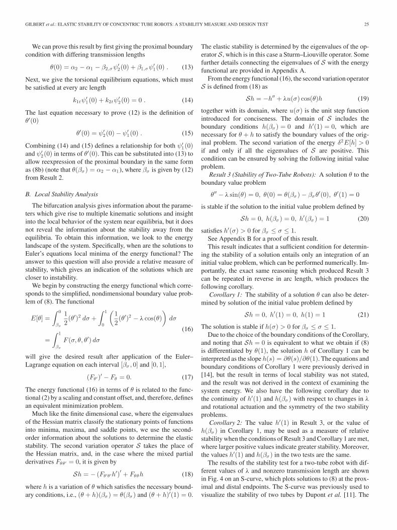
The following example shows how the stability theoryoutlined above has ramifications for motion planners andcontrollers. Existing approaches for dealing with solutionstability in motion planning methods have relied on thefact that the kinematic solutions are almost everywhere lo-cally continuous with respect to the set of variables q0 =[β1 . . . βn α1(β1) . . . αn (βn ) ]. However, from thestandpoint of the topology of the solutions, a much better choicefor planning purposes is the distal angles α1(L), . . . , αn (L),since this makes all components of the kinematic solutioncontinuous with respect to the set of configuration variablesqL = [β1 . . . βn α1(L) . . . αn (L) ]. Then, the mo-tion planning problem can be considered as finding continuous,admissible paths in both the physical space occupied by therobot and the configuration variable space.

Previously, without a test which could accurately determinethe stability of an arbitrarily chosen configuration qL , sampling-based planning methods could not guarantee that the resultingplanned trajectory is everywhere elastically stable. Fig. 9 shows,for a three-tube robot, how a continuous path in the distal anglespace remains continuous in the proximal angles, but the shapeof the trajectory becomes distorted when the relative stabilitymeasure approaches zero. If these distortions are allowed to be-come too large, then very small changes in the proximal relativeangles of the tubes can result in large but stable angular displace-ments at the distal end. Near these points of ill-conditioning,modeling errors or unpredictable external loads may make itpossible for the physical robot to snap.

At present, the relative stability measure is a heuristic thatindicates the solutions which are closer to instability; hence,we use the term “relative.” It is important to note that we havenot associated this measure with energetic units and have notproven bounds on how rapidly the measure can change acrossthe actuation space. In principle, the smallest eigenvalue of Scould give a more direct measurement of stability, but in practicethis quantity is much more difficult to compute.

One important consequence of the step from two tubes tothree tubes is that the third tube can actually provide paths inactuation space for the tubes to make complete rotations withrespect to one another without snapping, which would not bepossible with only two tubes. This effect exists for designs thatare beyond the bifurcation of the antialigned equilibria, butfor which the regions of instability in the rotational actuationspace have not yet connected. For circularly precurved tubes, we

suspect the growth of instability from the bifurcating equilibriais a fundamental property regardless of the number of tubes, butwe leave a proof of this to future study. For complex, nonplanartube designs, there may not exist any equilibria, and it is lessclear where instability will first arise; however, Result 5 stillpredicts the instability.

Note that the true rotational actuator space is of each anglemodulo 2π so that the opposite edges of the graphs in Fig. 10 areequivalent to one another. In the last plot of Fig. 10, the connec-tion between the unstable regions has prevented all paths whichtraverse complete relative rotations of any tube with respect toany other tube. In some cases, such a full rotation is possiblebetween one pair of tubes but not another pair.

Resolved-rate style control methods can also take advantageof the stability metric for redundancy resolution or for a sec-ondary weighted objective optimization. By computing or pre-computing the gradient of the stability metric,∇q det(H11(β)),resolved-rate methods can locally enforce a minimum stabilitymeasure to ensure that a relative margin of stability is maintainedfrom snapping configurations.

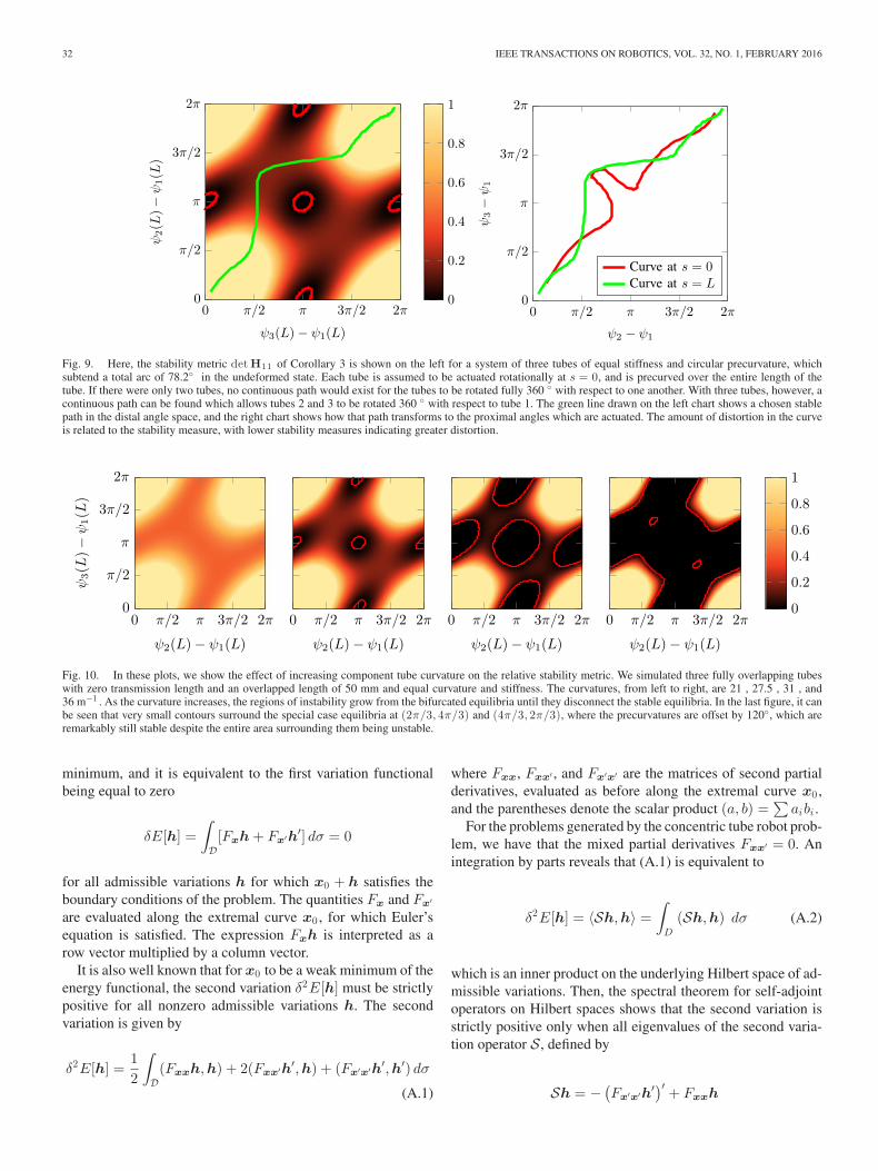
In terms of stability over the entire rotational actuation space,increasing transmission lengths and tube precurvatures tend tocontinuously destabilize the system. We show this effect by plot-ting the relative stability metric for every relative angle ψi − ψ1at the distal tip L. This space contains all possible configurationsup to a rigid body rotation. Fig. 10 shows how increases of thetube precurvature in a three tube robot cause instability to ariseat the equilibria with curvatures anti-aligned, and the regions ofinstability eventually grow until the space of stable tip rotationsbecomes disconnected, after which traversing the full relativerotation of any tube can only occur through a snap.

IX. CONCLUSION AND FUTURE WORK

In this paper, we have provided an analysis of bifurcation andelastic stability of unloaded concentric tube robots. This paperproposes an energy-based stability computation, which assignsa relative measure of stability to each configuration of the robot,which we believe will be useful for future research in control andmotion planning. We have also connected existing frameworksfrom the mechanics literature on Euler beams to concentric tuberobots. The bifurcation analysis enables a systematic, compu-tationally inexpensive, and closed-form algorithm for designersto create snap-free robots.

One important future advancement to the stability theory willbe the inclusion of externally applied loads so that motion plan-ning and control can incorporate stability information when theenvironmental interaction forces are large. Our results in this pa-per provide an approach to understanding concentric tube robotstability, and it is our hope that this study will facilitate theuse of high curvature concentric tube robot designs that werepreviously avoided.

APPENDIX ATHE SECOND VARIATION

In the calculus of variations, it is well known that Euler’sequation is a necessary but not sufficient condition for a


Fig. 9. Here, the stability metric det H11 of Corollary 3 is shown on the left for a system of three tubes of equal stiffness and circular precurvature, whichsubtend a total arc of 78.2◦ in the undeformed state. Each tube is assumed to be actuated rotationally at s = 0, and is precurved over the entire length of thetube. If there were only two tubes, no continuous path would exist for the tubes to be rotated fully 360 ◦ with respect to one another. With three tubes, however, acontinuous path can be found which allows tubes 2 and 3 to be rotated 360 ◦ with respect to tube 1. The green line drawn on the left chart shows a chosen stablepath in the distal angle space, and the right chart shows how that path transforms to the proximal angles which are actuated. The amount of distortion in the curveis related to the stability measure, with lower stability measures indicating greater distortion.

Fig. 10. In these plots, we show the effect of increasing component tube curvature on the relative stability metric. We simulated three fully overlapping tubeswith zero transmission length and an overlapped length of 50 mm and equal curvature and stiffness. The curvatures, from left to right, are 21 , 27.5 , 31 , and36 m−1 . As the curvature increases, the regions of instability grow from the bifurcated equilibria until they disconnect the stable equilibria. In the last figure, it canbe seen that very small contours surround the special case equilibria at (2π/3, 4π/3) and (4π/3, 2π/3), where the precurvatures are offset by 120◦, which areremarkably still stable despite the entire area surrounding them being unstable.

minimum, and it is equivalent to the first variation functionalbeing equal to zero

δE[h] =∫

D[Fxh + Fx′h′] dσ = 0

for all admissible variations h for which x0 + h satisfies theboundary conditions of the problem. The quantities Fx and Fx′

are evaluated along the extremal curve x0 , for which Euler’sequation is satisfied. The expression Fxh is interpreted as arow vector multiplied by a column vector.

It is also well known that for x0 to be a weak minimum of theenergy functional, the second variation δ2E[h] must be strictlypositive for all nonzero admissible variations h. The secondvariation is given by

δ2E[h] =12

∫

D(Fxxh,h) + 2(Fxx′h′,h) + (Fx′x′h′,h′) dσ

(A.1)

where Fxx, Fxx′ , and Fx′x′ are the matrices of second partialderivatives, evaluated as before along the extremal curve x0 ,and the parentheses denote the scalar product (a, b) =

∑

aibi .For the problems generated by the concentric tube robot prob-

lem, we have that the mixed partial derivatives Fxx′ = 0. Anintegration by parts reveals that (A.1) is equivalent to

δ2E[h] = 〈Sh,h〉 =∫

D

(Sh,h) dσ (A.2)

which is an inner product on the underlying Hilbert space of ad-missible variations. Then, the spectral theorem for self-adjointoperators on Hilbert spaces shows that the second variation isstrictly positive only when all eigenvalues of the second varia-tion operator S, defined by

Sh = −(

Fx′x′h′)′ + Fxxh


are positive.2 It is a prerequisite for the condition δ2E[h] > 0to be transformed into the condition on the eigenvalues of Sthat the eigenvectors of S form a complete orthonormal set forthe underlying Hilbert space. For the operators generated by theconcentric tube robot model, the eigenvectors of S do form sucha basis, as guaranteed by Theorem 1 of Dwyer and Zettl, whichsays that S is a self-adjoint operator [23]. The eigenvalue equa-tion Sψ = ρψ is a Sturm–Liouville eigenvalue problem, whichhas a countably infinite number of orthonormal eigenvectorswith eigenvalues that are all real and bounded below. Becausethere are an infinite number of eigenvalues, a direct computationwill not suffice for a feasible numerical test of stability.

Fortunately, continuous changes in Fxx, Fx′x′ , and the end-points of the interval D cause continuous changes in the spec-trum of S [27]. The basic idea for a numerical test is the follow-ing: If one can show that S has positive eigenvalues on someshortened domain which is a subset J ⊂ D, then the endpointsof J can be continuously varied to the endpoints of D, whilewatching for zero-crossings in the eigenvalues of S [17]. If Shas a zero eigenvalue for some choice of J , then we have anequation Sh = 0 on that domain with boundary conditions onh also satisfied at the endpoints of J .

If the problem has Dirichlet boundary conditions, it is wellknown that stability is determined by looking for conjugatepoints [24], and the conjugate point formulation and the eigen-value characterization have been shown to be equivalent [17],[28]. For concentric tube robots, the boundary conditions are notDirichlet, and, therefore, the conjugate point condition must bemodified. We must first verify that all the eigenvalues of S arepositive when the operator is taken to act on a shorter domain.For concentric tube robots, this means a shorter robot. Second,we look for conjugate points, which occur when Sh = 0 issolved for an admissible variation h, which is precisely whenS has an eigenvalue at zero. This two-part modification is ex-plained in detail by Hoffman et al. [16].

We are no longer guaranteed that a conjugate point resultsin an increase in the number of negative eigenvalues [17], be-cause the Neumann boundary condition, in general, preventsthe eigenvalues from being strictly decreasing functions of thedomain length. Nevertheless, we can still conclude that the ab-sence of a conjugate point implies positive eigenvalues, makingit a sufficient condition.

APPENDIX BPROOF OF RESULT 3

We define the family of related eigenvalue problems

Sφ = ρφ, φ(β) = 0, φ′(a) = 0 (B.1)

for the variable endpoint a, with β < a ≤ 1. It is known thatthe eigenvalues ρi , i = 1, 2, ..., move continuously with respectto continuous changes in a [17], [27]. The basic idea of thetest is that if there is a small enough a where all eigenvalues

2A technical note is that we consider only admissible variations, such thateach component of (Fx′x′h′)′ is absolutely continuous. For the concentric tuberobot kinematics, h represents a variation in the rotational angles of the tubes,the variation in moment is differentiable and has a continuous derivative.

are positive, then for an eigenvalue of the problem (B.1), witha = 1, to be negative, it must cross zero as a varies between βand 1. This condition can be checked with a simple test.

To look for an eigenvalue at zero in any of the related problems(B.1), we assume that zero is an eigenvalue with eigenvector hby setting Sh = 0, i.e., we set −h′′ + λ cos(θ)h = 0. It followsthat there exists an arc length σ for which Sh = 0, h(β) =0, and h′(σ) = 0. Since we do not know σ, we begin at theproximal boundary, where we know that h(β) = 0. Because Sis linear, the eigenvectors have arbitrary scale so that if h isan eigenvector, h′(β) may be arbitrarily chosen by scaling (hmust be nontrivial). We choose h′(β) = 1, and integrate thedifferential equation forward. In doing this, we have enforcedboth the differential form and the proximal boundary of theentire family of operators (B.1). If the distal boundary conditionh′(σ) = 0 is not satisfied for any σ, then zero is not an eigenvaluefor any of the operators of the family (B.1), contradicting theassumption of an eigenvalue at zero.

Since zero is not an eigenvalue for any of the problems, and ifthe problem has no negative eigenvalues for a sufficiently smallvalue of a, it is not possible that the boundary value problemon the whole interval has a negative eigenvalue by continuity ofthe spectrum with changes in the interval endpoint a.

To see that no eigenvalues are negative for small a, notethat S can be decomposed into S = T + Q, with T h = −h′′

and Qh = λ cos(θ)h. As a becomes smaller, it is known thatthe eigenvalues of T become larger. The operator Q can beseen as a perturbation of T , and when the eigenvalues of Tare made sufficiently large by choosing a sufficiently small, theperturbation Q, being bounded in magnitude, is incapable ofmoving an eigenvalue negative. The argument of this paragraphis made rigorously by Hoffman and Manning in [16].

APPENDIX CPROOF OF RESULT 5

We begin by showing that the eigenvalues of the problemare positive when the boundary conditions at L are moved tobe close to the boundary conditions at β. Here, the allowablevariation hi belongs to the space Di([βi, ai ]) = {f, (kitf

′) ∈AC([βi, ai ]) : f(βi) = 0, (kitf

′)(ai) = 0}, and the collectionh belongs to the Cartesian product D(S) = D1 × . . . ×Dn .Consider the eigenvalue problem, in which ai = βi + ε forsome small ε. Then, we still have the decomposition of S as inthe proof of Result 3 as S = T + Q. The operator T acts diag-onally on the hi , and so the eigenvalues γ of T h = γh may befound as the eigenvalues of n independent problems. The eigen-values are positive and the smallest eigenvalue can be madearbitrarily large by the choice of ε. Consider the extension of hi

to the whole interval [β, L], where it must be that h(β) = h(βi)and h′(L) = h′(βi + Li), since the two-point extension of (4)simulates the tubes as having infinite torsional stiffness andzero bending stiffness in the regions [β, βi ] and [βi + Li, L].The operator Q is identically the zero operator over the interval[β, βmax] due to the restriction of equation (6) and the formof Fψψ . The extended domain of the operator will be calledD[β ,L ](S). We will refer to h as the extension, since any


solution on the domain D(S) can be extended to a solution onthe domain D[β ,L ](S). The eigenvalues of S do not change dur-ing the extension to the left when all βi are moved to the left to β.The eigenvalues may change as all ai which are less than βmax

are increased to βmax, but all remain strictly greater thanzero since the equations are decoupled and still of the formT h = γh. Finally, the eigenvalues may change by a boundedamount as the ai are increased to βmax + ε, but by choiceof ε, we can guarantee that this change will not cause theeigenvalues to become negative. Thus, there is some domain forwhich the eigenvalues are all positive. As ai are then increasedtogether, ai = a → L, if an eigenvalue crosses zero we havea sub-problem on the interval [β, a] for which Sh = 0 has anon-trivial solution h, which is to say that there is a choiceof constants c with c = 0 so that H22(a)c = 0 and, therefore,h(s) = H12c is an eigenvector with eigenvalue zero. If, on theother hand, we do not have detH22(a) = 0 for any a, thenit must be that if zero is not an eigenvalue of Sh = 0 on anyinterval [β, a], and since the spectrum changes continuouslywith a, detH22 > 0 on the whole interval thus guarantees thatS has only positive eigenvalues on the whole domain [β, L].

The proof tacitly assumes that the eigenvalues move contin-uously with changes in the endpoint of the interval on whichS is defined, which is known to be true for the scalar Sturm–Liouville problem [27]. It is reasonable to assume this remainstrue for the matrix problem due to the fact that the resolventoperators of S on different domains with “close” endpoints areclose in precise sense. For a discussion of resolvent convergencein the context of Sturm–Liouville problems, see, for example,[29].

APPENDIX DCOMPUTATION OF THE STATE TRANSITION MATRIX eLΓe

First, assume that Γe is constant over some length L. Addi-tionally, assume that all tubes are present in this section. Then,use the change of coordinates y = T−1x, to yield

y′ = T−1ΓeTy = Qy (D.1)

where

Q =

[

0 V−1K−1t KtV

V−1K−1t AeV 0

]

=

[

0 I

Λ 0

]

. (D.2)

Compute the flow of the differential equation (D.1) over a lengthL as

y(L) = eLQy(0). (D.3)

The matrix exponential eLQ is given by

eLQ = G =

[

cosh(L√

Λ)√

Λ−1

sinh(L√

Λ)√

Λ sinh(L√

Λ) cosh(L√

Λ)

]

(D.4)where we define the hyperbolic trigonometric functions and thesquare roots to operate only on the diagonal elements of thematrix arguments. This equivalence can be shown by compar-ing the Taylor series expansions of eLQ and the Taylor series

expansions of the entries in G. Then, in the original coordinates,we have

x(L) = TGT−1x(0) (D.5)

as claimed.

ACKNOWLEDGMENT

The authors would like to thank A. Mahoney for criticalreview and many suggestions that improved the manuscript.

REFERENCES

[1] R. J. Hendrick, H. B. Gilbert, and R. J. Webster III, “Designing snap-freeconcentric tube robots: A local bifurcation approach,” in Proc. IEEE Int.Conf. Robot. Autom., 2015, pp. 2256–2263.

[2] W. Wei and N. Simaan, “Modeling, force sensing, and control of flexiblecannulas for microstent delivery,” ASME J. Dyn. Sys. Meas. Control,vol. 134, no. 4, pp. 041004-1–041004-12, 2012.

[3] N. V. Vasilyev, A. H. Gosline, A. Veeramani, G. P. Wu, M. T. Schmitz,R. T. Chen, A. Veaceslav, P. J. del Nido, and P. E. Dupont, “Tissue removalinside the beating heart using a robotically delivered metal mems tool,”Int. J. Robot. Res., vol. 34, no. 2, pp. 236–247, 2015.

[4] J. Burgner, D. C. Rucker, H. B. Gilbert, P. J. Swaney, P. T. Russell III,K. D. Weaver, and R. J. Webster III, “A telerobotic system for transnasalsurgery,” IEEE/ASME Trans. Mechatron., vol. 19, no. 3, pp. 996–1006,Jun. 2014.

[5] L. Torres, R. J. Webster III, and R. Alterovitz, “Task-oriented design ofconcentric tube robots using mechanics-based models,” in IEEE/RSJ Int.Conf. Intell. Robot. Syst., 2012, pp. 4449–4455.

[6] R. J. Hendrick, S. D. Herrell, and R. J. Webster III, “A multi-arm hand-held robotic system for transurethral laser prostate surgery,” in Proc. IEEEInt. Conf. Robot. Autom., 2014, pp. 2850–2855.

[7] C. Bergeles, A. H. Gosline, N. V. Vasilyev, P. J. Codd, P. J. del Nido,and P. E. Dupont, “Concentric tube robot design and optimization basedon task and anatomical constraints,” IEEE Trans. Robot., vol. 31, no. 1,pp. 67–84, Feb. 2015.

[8] H. B. Gilbert, D. C. Rucker, and R. J. Webster III, “Concentric tube robots:State of the art and future directions,” in Proc. 16th Int. Symp. Robot. Res.,2013, to be published.

[9] R. J. Webster III, J. M. Romano, and N. J. Cowan, “Mechanics ofprecurved-tube continuum robots,” IEEE Trans. Robot., vol. 25, no. 1,pp. 67–78, Feb. 2009.

[10] D. C. Rucker, B. A. Jones, and R. J. Webster, III,“A geometrically exactmodel for externally loaded concentric tube continuum robots,” IEEETrans. Robot., vol. 26, no. 5, pp. 769–780, Oct. 2010.

[11] P. E. Dupont, J. Lock, B. Itkowitz, and E. Butler, “Design and control ofconcentric-tube robots,” IEEE Trans. Robot., vol. 26, no. 2, pp. 209–225,Apr. 2010.

[12] J. Kim, D. Lee, K. Kim, S. Kang, and K. Cho, “Toward a solution tothe snapping problem in a concentric-tube continuum robot: Groovedtubes with anisotropy,” in Proc. IEEE Int. Conf. Robot. Autom., 2014,pp. 5871–5876.

[13] H. Azimian, P. Francis, T. Looi, and J. Drake, “Structurally-redesignedconcentric-tube manipulators with improved stability,” in Proc. IEEE/RSJInt. Conf. Intell. Robot. Syst., 2014, pp. 2030–2035.

[14] J. Ha, F. Park, and P. Dupont, “Achieving elastic stability of concentrictube robots through optimization of tube precurvature,” in Proc. IEEE/RSJInt. Conf. Intell. Robot. Syst., 2014, pp. 864–870.

[15] R. Xu, S. F. Atashzar, and R. V. Patel, “Kinematic instability in concentric-tube robots: Modeling and analysis,” in Proc. IEEE Int. Conf. Biomed.Robot. Biomechatron., 2014, pp. 163–168.

[16] K. Hoffman and R. Manning, “An extended conjugate point theory withapplication to the stability of planar buckling of an elastic rod subjectto a repulsive self-potential,” SIAM Math. Anal., vol. 41, pp. 465–494,2009.

[17] R. S. Manning, “Conjugate points revisited and Neumann–Neumann prob-lems,” SIAM Rev., vol. 51, no. 1, pp. 193–212, 2009.

[18] S. V. Levyakov and V. V. Kuznetsov, “Stability analysis of planar equilib-rium configurations of elastic rods subjected tosurname end loads,” ActaMechanica, vol. 211, no. 10, pp. 73–87, 2009.


[19] S. S. Antman, Nonlinear Problems of Elasticity, 2nd ed. New York, NY,USA: Springer-Verlag, 2005.

[20] T. Bretl and Z. McCarthy, “Quasi-static manipulation of a Kirchoff elasticrod based on a geometric analysis of equilibrium configurations,” Int.J. Robot. Res., vol. 33, no. 1, pp. 48–68, 2014.

[21] D. C. Rucker, R. J. Webster III, G. S. Chirikjian, and N. J. Cowan, “Equi-librium conformations of concentric-tube continuum robots,” Int. J. Robot.Res., vol. 29, no. 10, pp. 1263–1280, 2010.

[22] R. M. Murray, Z. Li, and S. S. Sastry, A Mathematical Introduction toRootic Manipulation. Boca Raton, FL, USA: CRC Press, 1994.

[23] H. I. Dwyer and A. Zettl, “Eigenvalue computations for regular matrixSturm–Liouville problems,” Electron. J. Differential Equations, vol. 1995,no. 5, pp. 1–13, 1995.

[24] I. M. Gelfand and S. V. Fomin, Calculus of Variations, R. A. Silverman,Ed. Mineola, NY, USA: Dover, 2000.

[25] J. Lock and P. E. Dupont, “Friction modeling in concentric tube robots,”in Proc. IEEE Int. Conf. Robot. Autom., 2011, pp. 1139–1146.

[26] A. R. Pelton, N. Rebel, T. W. Duerig, and A. Wick, “Experimental andFEM analysis of the bending behavior of superelastic tubing,” in Proc. 1stInt. Conf. Shape Memory Superelastic Technol., 1994, pp. 353–358.

[27] A. Zettl, Sturm–Liouville Theory. Providence, RI, USA: American Math-ematical Society, 2005.

[28] J. H. Maddocks, “Restricted quadratic forms and their application to bifur-cation and stability in constrianed variational principles,” SIAM J. Math.Anal., vol. 16, no. 1, pp. 47–68, 1985.

[29] P. B. Bailey, W. N. Everitt, J. Weidmann, and A. Zettl, “Regular approx-imations of singular Sturm–Liouville problems,” in Proc. Results Math.,1993, pp. 3–22.

Hunter B. Gilbert (S’10) received the B.S. degreein mechanical engineering from Rice University inHouston, TX, USA, in 2010. Since then, he has beenworking toward the Ph.D. degree in mechanical en-gineering at Vanderbilt University, Nashville, TN,USA, in the Medical Engineering and Discovery Lab-oratory. He is currently involved in the research onmedical robotics and continuum robotics. He receivedthe NSF Graduate Research Fellowship in 2012.

Richard J. Hendrick (S’12) received the B.S. degreein biomedical engineering from Texas A&M Univer-sity, College Station, TX, USA, in 2011. He is cur-rently working toward the Ph.D. degree in mechanicalengineering at Vanderbilt University, Nashville, TN,USA, and is involved in hand-held robotics, contin-uum robot design and control, and robotic endoscopicsurgery. He is currently with the Medical Engineer-ing and Discovery Laboratory. He received the NSFGraduate Research Fellowship in 2013.

Robert J. Webster III (S’97–M’08–SM’14) re-ceived the B.S. degree in electrical engineering fromClemson University, Clemson, SC, USA, in 2002, andthe M.S. and Ph.D. degrees in mechanical engineer-ing from The Johns Hopkins University, Baltimore,MD, USA, in 2004 and 2007, respectively.

In 2008, he joined the Faculty of VanderbiltUniversity. He is currently an Associate Professorof Mechanical Engineering, Electrical Engineering,Otolaryngology, Neurological Surgery, and UrologicSurgery, and directs the Medical Engineering and

Discovery Laboratory. He serves on the steering committee for the Vander-bilt Institute in Surgery and Engineering, which brings together physicians andengineers to solve challenging clinical problems. He is the Chair of the SPIEImage-Guided Procedures, Robotic Interventions, and Modeling Conference,and is an Associate Editor for IEEE TRANSACTIONS ON ROBOTICS. His re-search interests include surgical robotics, image-guided surgery, and continuumrobotics.

Dr. Webster received the IEEE Robotics & Automation Society Early CareerAward, the National Science Foundation CAREER award, the Robotics Scienceand Systems Early Career Spotlight Award, and the IEEE Volz Award.

Date post:	30-May-2018
Category:	Documents
Upload:	vunhan
View:	229 times
Download:	0 times

20 IEEE TRANSACTIONS ON ROBOTICS, VOL. 32,...

Documents