2nd, 3rd, 4th, 5th, And Higher Order IMD

Dallas Lankford, VII/19/1993, rev. IX/10/2015

A voltage version mathematical model of intermodulation distortion (IMD) takes the first few (often 4) terms ofthe Maclaurin series for the device under test (DUT) voltage transfer function,

Vout (Vin ) = V0 + k1Vin + k2 (Vin )2 + k3 (Vin)3,

and an input voltage

Vin = E l COS(w1t) + E 2 COS(w2t) ,

which is substituted into the Maclaurin series, and after application of trig identities for powers of COS,namely COS(x)COS(y) = (COS(x + y) + COS(x – y) )/2, COS2 (x) = (1 + COS(2x))/2, and COS3(x) = (3(COS(x) + COS(3x))/4, and rearrangement of terms, the following approximation of the output voltage Vout (Vin ), which we abbreviate Vout , can be constructed:

Vout = V0 + 1/2 k 2(E 12 + E 2

2 )

+ (k 1E 1 + 3/4 k 3E l3 + 3/2 k3E1E 2

2 ) COS(w1t)

+ (k 1E 2 + 3/4 k 3E 23 + 3/2 k3E1

2E2 ) COS(w2t)

+ 1/2 k 2E 12 COS(2wlt)

+ 1/2 k 2E 22 COS(2w2t)

+ k 2E 1E 2 COS((wl + w2)t)

+ k 2E 1E 2 COS((wl – w2)t)

+ 1/4 k 3E 13 COS(3wlt)

+ 1/4 k 3E 23 COS(3w2t)

+ 3/4 k 3E 12E 2 COS((2w1 + w2)t)

+ 3/4 k 3E 12E 2 COS((2w1 – w2)t)

+ 3/4 k 3E 1E 22 COS((2w2 + wl)t)

+ 3/4 k 3E 1E 22 COS((2w2 – wl)t).

My voltage version of IMD above was constructed from a similar development in “Don’t guess the spurious level of an amplifier. The intercept method gives the exact values with the aid of a simple nomograph,” by F. McVay, Electronic Design 3, February 1, 1967, 70 – 73.

As McVay said in his article (but did not show), if a dB/dB scale is used, then each IMD term can be expressed as a straight line (this is not entirely correct, the exceptions being the two fundamental (linear) terms as can be seen from the Maclaurin series expansion above, and the constant term which we shall omit by assuming that it is blocked by an output capacitor or transformer). When McVay said “dB/dB scale” he meant dB/dB coordinate system. Although McVay did not say it, the IMD terms can be expressed as straight lines only if the the tones are equal (E l = E 2 ). In addition, his article indicates that he knew that the IMD terms can also be expressed as straight lines in a dBm/dBm coordinate system (see the copy of one of McVay's graphs several pages below).

1

For a 2nd order example, let the IMD output voltage for the term k 2E 1E 2 COS((wl + w2)t) be denoted by Vout(f1

+ f2) . When the tones are equal let E = E 1 = E 2 , so that the RMS output voltage is VoutRMS(f1 + f2) =

1/sqrt(2) k2E2 , where sqrt(x) denotes the square root of x. T he output power in dB is Pout(f1 +

f2) = 10log([1/sqrt(2) k2E2]2 /50) = 10log([1/sqrt(2) k 2E2]2) – 10log(50) = 20log(sqrt(2) k 2) +

20log([1/sqrt(2)E]2) – 10log(50) = 20log(sqrt(2) k2) + 10log(50) + 2(10log([1/sqrt(2)E]2 /50)) . Thus Pout(f1 + f2) = 2(10log([1/sqrt(2)E]2 /50)) + 20log(sqrt(2) k2) + 10log(50) . This is a linear equation y = 2x +

b(f1 + f2) where x and y are the input and output powers respectively in dB and where b(f1 + f2) = 20log(sqrt(2)k2) + 10log(50) . The input and output terminations are taken as 50 ohms for convenience. We will often write b instead of b(f1 + f2).

The 2nd order dBm version is derived by adding 30 to both sides of the dB equation: y + 30 = 2x + b(f1 + f2) + 30so that y + 30 = 2(x + 30) + b(f1 + f2) – 30 . This is a linear equation equation y = 2x + bdBm(f1 + f2) where x

and y are the input and output powers respectively in dBm and bdBm(f1 + f2) = 20log(sqrt(2) k2) + 10log(50) – 30 . We will often write b instead of bdBm(f1 + f2) .

For a 3rd order example, when the tones are equal, the RMS output voltage for the 3/4 k 3E 12E 2 COS((2w1 + w2)t)

IMD term is VoutRMS(2f1 + f2) = 1/sqrt(2) 3/4 k3E3 . The output power in dB is Pout(2f1 + f2)) =

10log([1/sqrt(2) 3/4 k3E3]2 /50) = 20log(2 (3/4 k3)) + 20log([1/sqrt(2)E]3) – 10log(50) = 20log(2 (3/4 k3)) +

20log(50) + 3(10log([(1/sqrt(2)E]2 /50)) . Consequently Pout(2f1 + f2)) = 3(10log([(1/sqrt(2)E]2 /50)) + 20log(2 (3/4 k3)) + 20log(50) . This is a linear equation y = 3x + b(2f1 + f2) where x and y are the input and output powers respectively in dB, and b(2f1 + f2) = 20log(2 (3/4 k3)) + 20log(50) .

The 3rd order dBm version is derived by adding 30 to both sides of the dB equation: y + 30 = 3x + b(2f1 + f2) + 30 so that y + 30 = 3(x + 30) + b(dB) – 60 . This is a linear equation y = 3x + bdBm(2f1 + f2) where x and y are the input and output powers rescectivelyin dBm and bdBm(2f1 + f2) = 20log(2 (3/4 k3)) + 20log(50) – 60 .

It is now obvious from the derivations above that if the two tones are equal (E 1 = E 2) , then each 2nd order term of the Maclaurin series can be transformed into an equation of the form y = 2x + b with x and y in dB or x and y in dBm, and each 3rd order term of the Maclaurin series can be transformed into an equation of the form y = 3x +b with x and y in dB or x and y in dBm. In other words, the 2nd and 3rd order Maclaurin series terms are straight lines with slopes 2 and 3 respectively when a dB/dB or dBm/dBm coordinate system is used and the two tones are equal. Let us call these straight lines 2nd and 3rd order IMD straight lines.

If the DUT is linear with no constant term and no terms of order 2 or higher, then the voltage transfer function is

Vout = k1 Vin . For a single input voltage Vin = E COS(wt) the output voltage is Vout = k1 E COS(wt) , the RMS

output voltage is VoutRMS = 1/sqrt(2) k1 E and the dB power output is Pout = 10log([1/sqrt(2) k1 E]2 /50) =

20log(k1) + 10log([1/sqrt(2) E]2 /50) or y = x + 20log(k1) , and the dBm power output is y + 30 = x + 30 + 20log(k1) or y = x + 20log(k1) . Let G = 20log(k1) . G is called the gain of the DUT.

The dBm 2nd and 3rd order IMD straight lines intersect the straight line y = x + G where x and y are in dBm. The points of intersection are called 2nd and 3rd order intercepts for the 2nd and 3rd order cases respectively. The first coordinate of the point of intersection is called the input intercept point and the 2nd coordinate of the point of intersection is called the output intercept point. They are called points even though they are not points, but are coordinates. They are denoted IIP2, OIP2, IIP3, and OIP3, so that the points of intersection are denoted (IIP2,OIP2) and (IIP3,OIP3) respectively. A graph of the 3rd order case and some 3rd order relations are shown

2

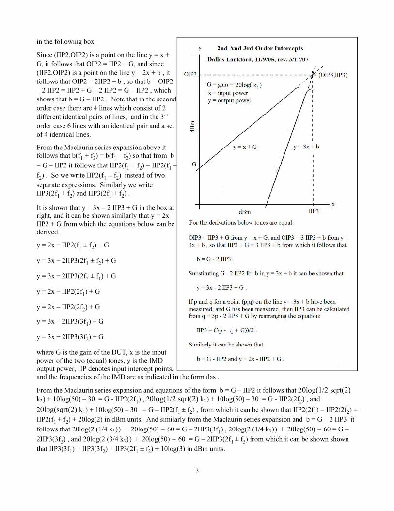
in the following box.

Since (IIP2,OIP2) is a point on the line y = x +G, it follows that OIP2 = IIP2 + G, and since(IIP2,OIP2) is a point on the line y = 2x + b , itfollows that OIP2 = 2IIP2 + b , so that b = OIP2– 2 IIP2 = IIP2 + G – 2 IIP2 = G – IIP2 , whichshows that b = G – IIP2 . Note that in the secondorder case there are 4 lines which consist of 2different identical pairs of lines, and in the 3rd

order case 6 lines with an identical pair and a setof 4 identical lines.

From the Maclaurin series expansion above itfollows that b(f1 + f2) = b(f1 – f2) so that from b= G – IIP2 it follows that IIP2(f1 + f2) = IIP2(f1 –f2) . So we write IIP2(f1 ± f2) instead of twoseparate expressions. Similarly we writeIIP3(2f1 ± f2) and IIP3(2f1 ± f2) .

It is shown that y = 3x – 2 IIP3 + G in the box atright, and it can be shown similarly that y = 2x –IIP2 + G from which the equations below can bederived.

y = 2x ¯ IIP2(f1 ± f2) + G

y = 3x ¯ 2IIP3(2f1 ± f2) + G

y = 3x ¯ 2IIP3(2f2 ± f1) + G

y = 2x ¯ IIP2(2f1) + G

y = 2x – IIP2(2f2) + G

y = 3x ¯ 2IIP3(3f1) + G

y = 3x ¯ 2IIP3(3f2) + G

where G is the gain of the DUT, x is the inputpower of the two (equal) tones, y is the IMDoutput power, IIP denotes input intercept points,and the frequencies of the IMD are as indicated in the formulas .

From the Maclaurin series expansion and equations of the form b = G – IIP2 it follows that 20log(1/2 sqrt(2) k2) + 10log(50) – 30 = G - IIP2(2f1) , 20log(1/2 sqrt(2) k2) + 10log(50) – 30 = G - IIP2(2f2) , and

20log(sqrt(2) k2) + 10log(50) – 30 = G – IIP2(f1 ± f2) , from which it can be shown that IIP2(2f1) = IIP2(2f2) =IIP2(f1 ± f2) + 20log(2) in dBm units. And similarly from the Maclaurin series expansion and b = G – 2 IIP3 it follows that 20log(2 (1/4 k3)) + 20log(50) – 60 = G – 2IIP3(3f1) , 20log(2 (1/4 k3)) + 20log(50) – 60 = G – 2IIP3(3f2) , and 20log(2 (3/4 k3)) + 20log(50) – 60 = G – 2IIP3(2f1 ± f2) from which it can be shown shown that IIP3(3f1) = IIP3(3f2) = IIP3(2f1 ± f2) + 10log(3) in dBm units.

3

Similarly, it can also be shown that IIP2(2f1) = IIP2(2f2 ) and that IIP3(3f1) = IIP3(3f2 ) .

McVay stated that the fundamental terms of the expansion were

k1E1 COS(w1t) and k1E2 COS(w2t) .

But that is clearly not correct. The fundamental terms are (k1E1 + 3/4 k3El3 + 3/2 k3E1E2

2 ) COS(w1t) and (k1E2 + 3/4 k3E2

3 + 3/2 k3E12E2 ) COS(w2t) . Perhaps McVay did not do a complete expansion of the cubic case. Or

perhaps he decided, for reasons known only to himself, that the additional coefficients of the fundamental terms were negligible.

Let us consider if the additional coefficients of the fundamental terms are negligible. In that regard, the COS(w1t) case is the following

(k 1E 1 + 3/4 k 3E l3 + 3/2 k3E1E 2

2 ) COS(w1t) ,

which may be regarded two output voltage terms at f1 , namely

k 1E 1COS(w1 t) and (3/4 k 3E l3 + 3/2 k3E1E 2

2) COS(w1t) .

It can be shown that the corresponding power equations in a dBm/dBm coordinate system are

y = x + G and y = 3x + bdBm(2f1 + f2) + 20log(3) .

The same equations can be derived for the COS(w2t) case.

From the above equations it follows that the additional terms of the linear cases of the Maclaurin series expansion are not contaminated by the additional coefficient terms as long as 20log(3) plus the output power in dBm of the graph of the 3rd order equation for 2f1 + f2 at input power x in dBm is sufficiently less than the output power in dBm of y = x + G for the same input power x . Let us take a few examples to determine if the contamination is significant. For the DUT with a single tone y = x + G at f1 and for the IMD case y = 3x – 2IIP3(2f1 + f2 ) + 20log(3) at f1 . These two powers are equal when x = 3x - 2IIP3(2f1 + f2 ) + 20log(3) . For an

amplifier with IIP3(2f1 + f2 ) = +30 dBm that is when x 25 . For the IMD to be 15 dBm less than the DUT

power, x 20 dBm. At x = 20, the DUT would typically be well beyond the 1 dB compression point, so for an amplifier with IIP3(2f1 + f2 ) = +30 dBm the linear terms will not be contaminated. For an amplifier with

IIP3(2f1 + f2 ) = +30 dBm , for the IMD power to be 15 dB less than the DUT power, x 2 dBm. In this case there might be some slight contamination near the 1 dB compression point.

The DUTs for McVay's development were BJTs, while the DUTs for my development above are arbitrary DUTs, including passive DUTs. Of course, McVay could have easily modified his development to include arbitrary DUTs. The primary contributions of my development are the relationships between and among the values of the various input intercepts, and the inclusion of how the log/log graphs of the fundamental (linear) terms differ slightly from straight lines. It is reasonable to assume that the relationships between and among the values of the various intercepts which I developed have been done by others long before I did them. But I have never seen such developments written down or even mentioned before in any publication.

Note that the relationships between and among the various output intercepts follow immediately from OIP3 = IIP3 + G . For example OIP3(2f1 + f2) = IIP3(2f1 + f2) + G , OIP3(2f1 – f2) = IIP3(2f1 – f2) + G , and IIP3(2f1 +f2) = IIP3(2f1 – f2) from which it follows that OIP3(2f1 + f2) = OIP3(2f1 – f2) .

Some writers, including manufacturers of amplifiers, do not identify which intercepts they are writing about but merely write, for example, IP3 without stating whether it is the input or output intercept. This is, of course, undesirable. In my opinion, manufacturers of amplifiers do this to mislead potential buyers into thinking that the

4

amplifier(s) they are buying have better strong signal performance than they actually do.

I vaguely recall struggling with McVay's intercept concept when I first encountered it. Deriving the approximation of the output transfer function from the first few terms of the Maclaurin series approximation of the transfer function was straightforward. But my further developments of the intercept method beyond that point were not well done at that time, perhaps not even correctly done, and though I believe that I wrote up a development at that time, I recall that I eventually deleted that development because I was not satisfied with it. The 2005 date of my development of the formulas in the box above whose main objectives were the third order formula y = 3x – 2IIP3 + G and the second order formula y = 2x – IIP2 + G suggests that it took me some time to find a satisfactory development of the intercept method beyond the Maclaurin series expansion. As I recall, I developed the formulas in the box considerably earlier than 2005, but did not put them in an article before 2005. It is difficult to say whether I had a clear understanding at that time of McVay's log/log construction from which he derived the linear equations y = 2x + b and y = 3x + b. What does seem clear now is that it was not immediately obvious to me how to derive such equations. Otherwise it would not have taken me considerably more than a few minutes to rediscover (?) those derivations today (III/31/2015).

It may seem surprising that it has taken me over 20 years to develop a correct and relatively complete article about my voltage version of McVay's intercept concept. But thoroughly understanding McVay's article and its consequences were not high priorities for me. I spent virtually all of my time on other matters, including developing high performance IMD measurement systems, building and testing high performance amplifiers (including Norton transformer feedbackamplifiers), building and testing phasers, usingEZNEC to design phased arrays of antennas for theMW band, building and testing phased arrays inmy yard, going on DXpeditions to test the antennaarrays I designed, and so on. Had it not been forDave Leeson emailing me a few days ago asking ifI had a copy of McVay's paper, it is unlikely that Iwould taken another look and McVay'sdevelopment and completed my development ofmy voltage version of McVay's intercept concept.It has been very satisfying to work on McVay's 2nd

and 3rd order intercept concepts again, andespecially to complete work I started long ago.

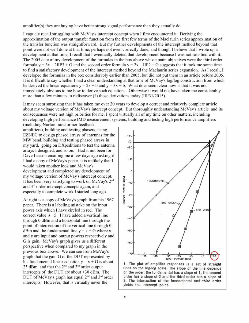
At right is a copy of McVay's graph from his 1967paper. There is a labeling mistake on the inputpower axis which I have circled in red. Thecorrect value is +5. I have added a vertical linethrough 0 dBm and a horizontal line through thepoint of intersection of the vertical line through 0dBm and the fundamental line y = x + G where xand y are input and output powers respectively andG is gain. McVay's graph gives us a differentperspective when compared to my graph in theprevious box above. We can see from McVay'sgraph that the gain G of the DUT represented by his fundamental linear equation y = x + G is about25 dBm. and that the 2nd and 3rd order outputintercepts of the DUT are about +30 dBm. TheDUT of McVay's graph has equal 2nd and 3rd orderintercepts. However, that is virtually never the

5

case. Below his graph, McVay said “3. The intersection of the fundamental and third order yields the intercept point.” Since his second and third order points of intersection are equal, his statement is correct. Of course, in general the second and third order intercept points are not equal, as I said above. So in general a DUT will have two separate intercepts, a second order intercept and a third order intercept.

At right is another graph based on a push-pull Nortontransformer feedback amplifier which I designed. It hadgain G 10 , IIP2(f1 ± f2) +80 dBm, and IIP3(2f1 ± f2)

+30 dBm where means “is approximately equal to”.The axes of this coordinate system are in dBm. These 2nd

and 3rd order lines are typical of a very good amplifier.The graphs in the two boxes above are idealized graphsbecause for real DUTs the lines do not extend indefinitelyfor higher powers. Real world DUTs have 1 dBcompression points where the lines curve into horizontallines. The graphs in the box at right are approximationsfor what is observed in the real world.

Intercepts are often measured with tones on the order of –120 dBm . With (equal) tones of –20 dBm , it can beshown that the y coordinate (output IMD) is –110 dBm .When measuring IIP2 and IIP3, I usually did not find thepoint of intersection of the 2nd and 3rd order straight linefor the DUT which I was measuring because I did notknow IIP2 and IIP3 in advance. I would merely beginwith (equal) tones on the order of –20 dBm and adjustthe tones until I got IMD on the order of –110 dBm .Next I would measure the gain of the DUT. Then I wouldcalculate IIP2 and IIP3 using the formulas

IIP2 = 2p – q + G where p is the measured tone valueand q is the measured IMD value for the 2nd order IMD,and

IIP3 = (3p – q + G ))/2 where p is the measured tonevalue and q is the measured IMD value for the 3rd orderIMD .

McVay also discussed the case when the tones are not equal. When tones are not equal, two dimensional dB/dB and dBm/dBm coordinate systems can no longer be used. In those cases, it can be shown that the output power

Pout is a function of two input powers, namely the input power for E 1 and the input power for E 2 and that, for example, in the case of the IMD term k 2E 1E 2 COS((wl + w2)t) the dB/dB equation is y = x1 + x2

+ 20log(sqrt(2) k2) + 10log(50) where x1 and x2 are the input powers in dB for the unequal tones (inputs) E l COS(wlt) and E 2 COS(w2t) respectively. The “dBm equation” is y = x1 + x2 + 20log(sqrt(2) k2) + 10log(50) – 30 . A similar result y = 2x1 + x2 + 20log(2 (3/4 k3)) + 20log(50) , where x and y are the input and output powers respectively in dB, can be derived for the 3rd order case 2f1 + f2 .

So when tones are not equal, the 2nd and 3rd order IMD power equations are not equations of straight lines, but are equations of surfaces in three dimensional coordinate systems.

A nice feature of the DSA815-TG is that it permits you to save a “capture” .bmp file of the display to a USB memory stick. The graphic below is the result of such a “capture”. The IMD frequencies are easily read off of the display capture. The minimum resolution bandwidth (RBW) is 100 Hz. According to one reviewer, the

6

version of the Rigol DSA815-TG sold in China includes a 10 Hz RBW. That would be nice to have because it would lower the noise floor by about another 10 dB and perhaps make weaker IMD appear.

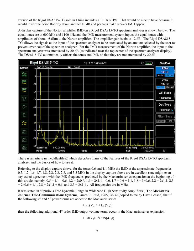
A display capture of the Norton amplifier IMD on a Rigol DSA815-TG spectrum analyzer is shown below. The equal tones are at 600 kHz and 1100 kHz and the IMD measurement system inputs the equal tones with amplitudes of about –6 dBm to the Norton amplifier. The amplifier gain is about 12 dB. The Rigol DSA815-TG allows the signals at the input of the spectrum analyzer to be attenuated by an amount selected by the user to prevent overload of the spectrum analyzer. For the IMD measurement of the Norton amplifier, the input to the spectrum analyzer was attenuated by 20 dB (as indicated near the top center of the spectrum analyzer display). The DSA815-TG automatically offsets the tones and IMD so that they are not attenuated by 20 dB.

There is an article in thedallasfiles2 which describes many of the features of the Rigol DSA815-TG spectrum analyzer and the basics of how to use it.

Referring to the display capture above, for the tones 0.6 and 1.1 MHz the IMD at the approximate frequencies 0.5, 1.2, 1.6, 1.7, 1.8, 2.2, 2.3, 2.8, and 3.3 MHz in the display capture above are in excellent (one might even say exact) agreement with the IMD frequencies predicted by the Maclaurin series expansion at the beginning of this article, namely, 0.5 = 1.1 – 0.6, 1.2 = 2x0.6, 1.6 = 2x1.1 – 0.6, 1.7 = 0.6 + 1.1, 1.8 = 3x0.6, 2.2 = 2x1.1, 2.3 = 2x0.6 + 1.1, 2.8 = 2x1.1 + 0.6, and 3.3 = 3x1.1 . All frequencies are in MHz.

It was stated in “Spurious Free Dynamic Range in Wideband High Sensitivity Amplifiers”, The Microwave Journal, Tele-Communications Systems, James R. Reid, 1965, 26-32 (copied to me by Dave Leeson) that if the following 4th and 5th power terms are added to the Maclaurin series

+ k 4 (Vin )4 + k 5 (Vin)5

then the following additional 4th order IMD output voltage terms occur in the Maclaurin series expansion:

+ 1/8 k 4E 14 COS(4wlt)

7

+ 1/8 k 4E 24 COS(4w2t)

+ 3/4 k 4E 12E 2

2 COS((2w1 2w2)t)

+ 1/2 k 4E 13E 2 COS((3w1 w2)t)

+ 1/2 k 4E 1E 23 COS((3w2 w1)t)

and the following additional 5th order output terms are contained in the Maclaurin series expansion:

+ 1/16 k 5E 15 COS(5wlt)

+ 1/16 k 5E 25 COS(5w2t)

+ 5/16 k 5E 14E 2 COS((4w1 w2)t)

+ 5/16 k 5E 1E 24 COS((4w2 w1)t)

+ 5/8 k 5E 13E 2

2 COS((3w1 2w2)t)

+ 5/8 k 5E 12E 2

3 COS((3w2 2w1)t) .

Referring to the Rigol DSA815-TG display capture above, the IMD at 0.7, 1.0, 2.4, 2.7, 2.9, and 3.4 MHz are IMD predicted by the order 4 terms of the Maclaurin series expansion, and the IMD at 1.3, 2.1, and 3.5 MHz areIMD predicted by the order 5 terms of the Maclaurin series expansion.

The IMD at 3.1 MHz does not agree with 2nd, 3rd, 4th or 5th order, but it does agree with 3.1 = 5x1.1 – 4x0.6 which is 9th order.

As was shown above for the 2nd and 3rd order cases, when the two tones are equal and the 4th and 5th order power equations are plotted on a two dimensional dBm/dBm coordinate system, the equations are linear with slopes 4 and 5 respectively. The intersections of those graphs with the line y = x + G may be defined to be 4 th and 5 orderintercepts respectively which are denoted OIP4, IIP4, OIP5, and IIP5. As shown for the 2nd and 3rd order cases, the following two equations can be derived for the 4th and 5th order cases

y = 4x – 3IIP4 + G and y = 5x – 4IIP5 + G ,

from which IIP4 and IIP5 can be calculated from measurements. To illustrate how IIP3, IIP4, and IIP5 can be calculated from measurements, we begin with IIP3.

For IMD3 at 2f2 – f1 take y = 3x – 2IIP3(2f2 – f1) + G so that from the display capture above –71 = 3(–6) – IIP3(2x1.1 – 0.6) + 12 (subtracting 25 from the –48 dBm on the display capture because of the low level inaccuracy of the DSA815-TG as described above), and 2IIP3(2x1.1 – 0.6) = 48 – 18 + 12 = 42, and so IIP3(2x1.1 – 0.6) +21 dBm (positive intercepts are traditionally expressed with a + in front of the positive intercept value). This value of IIP3 puzzles me because in the past I have measured the IIP2 of this push-pull Norton transformer feedback amplifier many times as about +35 dBm. Did I make a mistake (the same mistake every time) previously, or is there something wrong with my current IMD measurement system which uses the dual outputs of a Rigol DG4062 function generator and a Rigol DSA815-TG? I have also observed when using the current measurement system that the 3rd order IMD from the Norton amplifier does not decrease by exactly 30 dB for every 10 dB decrease of the tones. Also, the calculated values of IIP3 to decrease as the tones are decreased. Does this mean that the slope of the IMD3 line for the Norton amplifier is not exactly 3, or again, is there something wrong with my current IMD measurement system? I do not know. Similarly it can be shown that IIP4(3x1.1 – 0.6) +21 dBm and IIP5(3x1.1 – 2x0.6) +15 dBm using the display capture above.

When I saw all the 4th and 5th order IMD on the DSA815-TG display, I was rather surprised. Of course, the tonesdo not have to be reduced much (about 10 or 12 dB) for the 4th and 5th order IMD to vanish below the noise floor of the amplifier. Nevertheless, a pair of big signals, approaching 0 dBm, can generate some rather hefty 4 th and

8

5th order IMD. I vaguely recall noticing other spurious responses as I was measuring IIP2 and IIP3 of amplifiers with my IMD measurement systems in the past. But it never occurred to me to try to determine the causes of theother spurious responses or that the other spurious responses might be 4th and 5th order IMD.

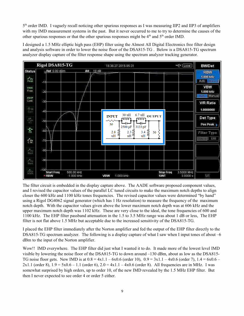
I designed a 1.5 MHz elliptic high pass (EHP) filter using the Almost All Digital Electronics free filter design and analysis software in order to lower the noise floor of the DSA815-TG . Below is a DSA815-TG spectrum analyzer display capture of the filter response shape using the spectrum analyzer tracking generator.

The filter circuit is embedded in the display capture above. The AADE software proposed component values, and I revised the capacitor values of the parallel LC tuned circuits to make the maximum notch depths to align closer the 600 kHz and 1100 kHz tones frequencies. The revised capacitor values were determined “by hand” using a Rigol DG4062 signal generator (which has 1 Hz resolution) to measure the frequency of the maximum notch depth. With the capacitor values given above the lower maximum notch depth was at 606 kHz and the upper maximum notch depth was 1102 kHz. These are very close to the ideal, the tone frequencies of 600 and 1100 kHz. The EHP filter passband attenuation in the 1.5 to 3.5 MHz range was about 1 dB or less, The EHP filter is not flat above 1.5 MHz but acceptable due to the increased sensitivity of the DSA815-TG.

I placed the EHP filter immediately after the Norton amplifier and fed the output of the EHP filter directly to the DSA815-TG spectrum analyzer. The following is a display capture of what I saw when I input tones of about –6dBm to the input of the Norton amplifier.

Wow!! IMD everywhere. The EHP filter did just what I wanted it to do. It made more of the lowest level IMD visible by lowering the noise floor of the DSA815-TG to down around –130 dBm, about as low as the DSA815-TG noise floor gets. New IMD is at 0.8 = 4x1.1 – 6x0.6 (order 10), 0.9 = 3x1.1 – 4x0.6 (order 7), 1.4 = 6x0.6 – 2x1.1 (order 8), 1.9 = 5x0.6 – 1.1 (order 6), 2.0 = 4x1.1 – 4x0.6 (order 8). All frequencies are in MHz. I was somewhat surprised by high orders, up to order 10, of the new IMD revealed by the 1.5 MHz EHP filter. But then I never expected to see order 4 or order 5 either.

9

Below is a DSA815-TG display capture of the toroid version of the 1.5 MHz EHP filter being fed 600 kHz and 1100 kHz tones at –6 dBm. The Norton amplifier is NOT in the signal path for the display below.

There is not much to see. A very weak spur of about –125 dBm at about 900 kHz is an internal spur of the spectrum analyzer. Whether the other “blips” are spurs, IMD, or just noise floor anomalies I do not know. This shows that the 1.5 MHz EHP filter is IMD free down to about –130 dBm or lower.

10

I actually built two versions of the 1.5 MHz EHP filter, one entirely with air core inductors, and one entirely with toroid inductors using iron-powder toroids (a T-106-2 toroid for the 30 uH inductor and four T-50-2 toroidsfor the smaller value inductors). I wanted the 1.5 MHz EHP filter to be free of IMD for tones near 0 dBm. I built the air core version first, hoping it would be IMD free. It was... no IMD for tones up to –6 dBm. Next, I built the iron-powder toroid version, and found that it was also IMD free for tones up to –6 dBm. Since toroids take up less space, the toroid version was my choice for the final version.

The EHP 1.5 MHz filter was built in aHammond 1590C aluminum box as shown atright. The box has many extra holes becauseit is a “recycled” box (I try not to let thingsgo to waste... the extra holes can be coveredup with thin sheets of aluminum screwed tothe sides of the box). This filter is the iron-powder toroid version. The 4 small toroidsare Amidon T-50-2 and the large toroid isAmidon T-106-2. The correct inductanceswere obtained by using an Almost All DigitalElectronics L/C Meter IIB. The small toroidsare self-supporting with an adhesive backed 3/4 inch thick rubber strip underneath toprevent toroid contact with the metal box...just in case. Similar rubber strips wereplaced in the top of the Hammond box. Thelarger toroid is sandwiched between twosquares of plexiglass which provides secure support and prevents contact with the metal box. There is a 1/2 inchinsulated standoff with pronged solder lug on top which is used for soldering together the middle leads of the capacitor pairs. The end leads of the capacitors are soldered directly to the BNC center conductors. The correct values of the capacitors are obtained by soldering pairstogether. The filter ground is a #18 solid tinned wire runningfrom the shell (ground) of the input BNC connector to theshell (ground) of the output BNC connector.

At right is the exterior of the recycled Hammond 1590C boxcontaining the 1.5 MHz Elliptic High Pass Filter with thinsheets of aluminum covering the holes in the sides of therecycled box (and screws in the top of the box covering screwholes) and with appropriate labels on top of the box.Previously I thought that the 1.5 MHz Elliptic High PassFilter was not symmetric, that the filter response differeddepending on which BNC connector was used for input. Butsubsequent observations indicated that is not the case.Nevertheless, I will continue to use the “left to right”orientation of the schematic with INPUT as the left hand sideand OUTPUT as the right hand side of the schematic. Myinclination is better safe than sorry.

Curiously, when using my DSA815-TG spectrum analyzer the slopes of the IMD straight lines in the dB/dB and dBm/dBm coordinate systems are not exactly 2 and 3 as predicted by theory. It is possible that the IMD slope inaccuracy is due to inaccurate IMD amplitudes of the DSA815-TG spectrum analyzer when multiple tones are input to the DSA815-TG. However, my Tektronix 495P spectrum analyzer has similar amplitude inaccuracy. I do not know what to make of this.

11